1  

WELCOM

User Manual1

Version 2.0

Abdelkrim Araar2, Sergio Olivieri,3 Carlos Rodriguez-Castelan4 and Eduardo Malasquez5

Abstract

This User Manual presents the WELCOM Stata tool. The Global Solutions Group on Markets and

Institutions for Poverty Reduction and Shared Prosperity at the Poverty and Equity Global Practice

has developed WELCOM, a novel microsimulation tool that estimates distributional effects of

changes in market structure (e.g. a move from monopoly to more competitive markets) which could

be induced through regulatory reform or easing of trade barriers. The WELCOM tool is a software

interface that requires data from household surveys, particularly households’ consumption of

different goods and services, as well as information about market structure in the relevant sectors,

to assess how changes in prices affect the welfare of households along the income/consumption

distribution. In addition, the tool relies on a poverty line and a relevant welfare aggregate (income

or consumption) to assess first-order effects on poverty indicators such as headcount and poverty

gap, in addition to changes in inequality.

                                                            1 WELCOM is a product of the World Bank. 2 University of Laval, Quebec City. 3 World Bank, Washington DC. 4 World Bank, Washington DC. 5 World Bank, Washington DC. 

 

2  

Acknowledgements

This research was sponsored by The World Bank. The authors gratefully acknowledge the

guidance of Tara Vishwanath, and helpful comments received from members of the Global

Solutions Group of Markets and Institutions for Poverty Reduction at the Poverty and Equity

Global Practice.

List of Acronyms and Abbreviations

CEA—Counsel of Economic Advisers

CD—Cobb-Douglass function

CES—Constant elasticity of substitution utility function

CMA—Competition and Markets Authority

FGT—Foster-Greer-Thorbecke class of poverty measures

GP—Global Practice

GSG—Global Solutions Group

PCO—Partial Collusive Oligopoly

PERC—Perfect Competition

WB—The World Bank

 

3  

Contents

Acknowledgements ........................................................................................................................ 2 

List of Acronyms and Abbreviations ........................................................................................... 2 

1.  Introduction ........................................................................................................................... 4 

2.  WELCOM Models ................................................................................................................ 7 

2.1  The theoretical framework of the mcwel Stata module ................................................... 7 

2.2  Market concentration structure and prices ....................................................................... 8 

a.  Monopolistic structure ..................................................................................................... 9 

b.  Oligopolistic Cournot-Nash equilibrium structure ....................................................... 12 

c.  Partial collusive oligopolistic structure ........................................................................ 16 

d.  Partial market adjustment ............................................................................................. 21 

2.3  Price changes and the household well-being ................................................................. 22 

a.  The Laspeyres measurement .......................................................................................... 23 

b.  The equivalent variation measurement .......................................................................... 23 

c.  The compensated variation measurement ..................................................................... 24 

2.4  Market structure and prices changes: a brief empirical example .................................. 24 

3.  WELCOM Stata Package and the market concentration and wellbeing tool ............... 25 

3.1  Installation ..................................................................................................................... 25 

3.2  The mcwel module for Stata ........................................................................................ 28 

a.  Preparing the dataset .................................................................................................... 29 

b.  Launch the mcwel dialog box ........................................................................................ 31 

c.  The “Main” tab ............................................................................................................. 32 

d.  The “Items” tab ............................................................................................................. 42 

e.  The “Table Options” tab ............................................................................................... 44 

f.  The “Graph Options” tab ............................................................................................. 45 

g.  The “if/in” tab ............................................................................................................... 46 

3.3  The mcwel outputs ....................................................................................................... 47 

3.4  Examples of the mcwel tool ......................................................................................... 49 

References .................................................................................................................................... 56 

 

 

4  

1. Introduction

This User Manual presents the WELCOM module, a tool build on Stata to analyze the

potential distributional impacts produced by changes in competition conditions either in specific or

multiple markets. In general, analyzing the welfare effects of policy reforms aimed at correcting

market imperfections is not a simple task, especially when the potential distributional impacts of

such policies need to be assessed prior to their implementation. Market imperfections not only

reduce economic efficiency and social welfare in both developed and developing countries, but

recent economic literature suggest that market imperfections are more pernicious for households at

the bottom of the income distribution (Urzua, 2013; Busso and Galiani, 2015; and Atkin et al.,

2016).6

Market imperfections affecting competition can take multiple forms such as collusive

arrangements among firms with market power,7 vertical or horizontal agreements limiting

competition at different stages of the production or distribution chain,8 legal barriers to entry or exit

markets,9 prohibitive tariffs on imports and exports, statutory monopolies and price controls, among

others. This User Manual focuses in market imperfections affecting the conditions for competition

in specific markets or industries10 such as anticompetitive behaviors by firms and government

restrictions, and in the effects of development policies aimed at fostering competition.

Interventions to correct market imperfections and, more specifically, policy reforms to

foster competition can have mixed effects in household’s welfare given the different roles played

by households in the economy as consumers, employees and producers. First, competition policy

reforms can affect the overall conditions of competition between firms in the market, affecting

                                                            6 In spite that we use the term “income distribution,” we could also organize and rank households based on their level of consumption or wealth, producing analysis based on consumption distribution or wealth distributions, respectively. 7 Harrington (2017) argues that collusive agreements occur when firms in a market coordinate their behavior to produce a supracompetitive outcome. 8 For a survey on the determinants and effects of vertical integration se Perry (1989). 9 Barriers to entry generally refer to any form of advantages that have accrued to incumbents over time such as demand-side network effects (i.e. the quality of a product or service increases with the number of users), increased economies of scale that make harder for entrants to compete, or those created by successful political lobbying, among others (Furman, 2016). 10 One non-exhaustive classification of potential anticompetitive conducts includes: (i) horizontal agreements or collusion practices such as price or geographical cartels; (ii) vertical restraints or vertical mergers like exclusive supply contracts; and (iii) other abusive practices such as predatory pricing, bundling and tying, refusal to supply, raising rival’s costs and price discrimination (Motta, 2010). Also, notice that none of these practices are necessarily anti-competitive per se, since they could also be a consequence of a legitimate strategic response to specific market conditions; therefore, they should be independently analyzed by competition authorities.

 

5  

household’s wellbeing in their role as consumers through changes in prices, quality and diversity

of alternatives available for purchase (Atkin et al., 2016; Begazo and Nyman, 2016). In addition,

competition reforms can affect household’s wellbeing in their role as employees as well as

producers of good and services. For instance, competition reforms may affect the nominal wages

perceived by workers, the number and composition of firms demanding labor—due to the potential

entry or exit of firms—affecting employees bargaining power, the presence of oligopsonies in

factor markets such as labor, or the consolidation of firms (CEAb, 2016). Moreover, competition

policy reforms also affect household welfare through their effects on capital gains due to changes

in firms’ profits due to more intense competition or affecting small firms exposure to

anticompetitive behavior from larger rivals (Outreville, 2015).11 Furthermore, market power is also

a source of production misallocation, resulting in welfare losses for the overall economy, since

output ends up being produced in higher-cost (less productive) units of production, and less output

in more efficient production units of the economy (Bridgman et al., 2015; Asker et al., 2017).

The impacts of competition policy interventions are often conditional on the initial

characteristics of the market or industry under analysis as well as on the effective regulatory and

competition framework following the intervention. Thus, the analysis of the conditions of

competition in markets typically involves more than meets the eye. For instance, an increase in

revenue concentration is neither necessary nor sufficient to indicate increases in market power;

higher prices can either be a signal of quality or of a lack of competition; similar price movements

can be evidence of either efficiency or of a cartel; and neither concentration nor large market share

equal market power nor dominance (Gonzalez, et al 2015; Furman, 2016). Thus, each policy should

be evaluated on its own merits, and understanding what influences the observed market outcomes

and how business behave and interact in the market should be a priority.12

In addition, notice that the policy reforms under study involve a broad set of government

interventions and private agent behaviors that can affect the functioning of markets. Moreover, this

User Manual does not deal with the question of what type of behavior constitutes an abuse of market

power or what are the best policies to remedy it (see Motta, 2004; or Buccirossi, 2008 for

                                                            11 The body of early literature in industrial organization known as the Structure-Conduct-Performance (SCP) hypothesis argues that there is a relationship between market concentration and firm profitability (Bain, 1951). For instance, according to the SCP theory dominant firms in concentrated markets are more capable of setting prices through collusion and, therefore, earn extraordinary profits. Later approaches such as the Relative-Market-Power (RMP) and the Efficient Structure (ES) also argued that market structure affects the market competition among firms (Outreville, 2015). 12 This approach is analogous to the “rule of reason” in antitrust, that appeals to a rigorous analysis of how markets work, taking into account the specificities of particular industries; in contrast to the “per se rules”, where certain behaviors are mechanically allowed or prohibited (Tirole, 2015).

 

6  

discussions on these topics), but instead focuses on the distributional impacts of the policy

interventions or changes in competitive conditions affecting competition in specific markets, taking

the policies or behaviors under analysis as given.

Three common examples how the behavior of private firms affect competition are: (i)

through the creation and exploitation of market power by individual firms, (ii) the joint exploitation

of market power by a group of firms, and (iii) the partial or total exclusion of competitors from

markets to create or protect the market power of a dominant or dominants firms (Buccirossi, 2008).

Since competition policy reforms can have mixed impacts in households, given the institutional

characteristics of the markets, the identification of the overall effects of these policies must hinge

on the individual analysis of each reform or competition policy.

The User Manual for the WELCOM13 package is part of a larger effort by the World Bank

to generate knowledge to improve the understanding of the links among competition, growth and

shared prosperity as well as to promote policies that foster competition, especially in developing

countries. This Manual currently focuses on the mcwel tool for Stata—the first step of a more

comprehensive project to provide a menu of flexible and user-friendly tools to analyze the effects

of market imperfections in well-being—and is divided into five main sections. The first section is

a general introduction that helps to motivate the importance of this User Manual, of the WELCOM

package. In the second section, this Manual discusses the importance of competition policy

reforms, discusses a general theoretical framework and relevant empirical studies on the

relationship between competition and poverty and inequality. In section three, the User Manual

shows the theoretical framework underlying the alternative methods of analysis available in the

tool. This version of the tool focuses on the study of the potential distributional impacts of market

concentration in consumer welfare through the prices channel. The forth section presents the

WELCOM package for Stata and how it can be used as well as examples to interpret the outputs of

the package. In the medium term the team plans to integrate additional modules to analyze the

impact of the trade liberation and especially the entry of the foreign distribution chains on well-

being.

                                                            13 Welfare and Competition (WELCOM). 

 

7  

2. WELCOM Models Section 2 of this user Manual discusses the theoretical framework, assumptions and data

requirements of the tool. First, Section 3 discusses the theoretical underlying WELCOM. Then,

this Section discusses the three alternative market structures—a monopolistic structure, an

oligopolistic market with firms involved in a Cournot-type competition14 and an oligopolistic

market with collusion among the dominant firms (firms with largest market share)—available in

the tool, their key assumptions and their associated equilibria. Finally, the third part of Section 3

discusses three alternative monetary measures of well-being that can be estimated using the tool

and briefly presents an empirical example.

2.1 The theoretical framework of WELCOM

The current version of the WELCOM toolkit includes the mcwel command that was

designed to help assess the impact of competition policy reforms on consumer prices. Thus,

WELCOM presents an absolute and relative incidence analysis of the effects of competition

reforms (i.e., changes in market power) on consumer welfare operating through the prices

mechanism. A second stage of the tool is expected to introduce the potential impacts of market

power on welfare through the labor market channel.

In competitive markets firms behave as price takers which are unable to affect equilibrium

prices through their individual actions15 (other assumptions of the competitive markets include the

private nature of goods and services, free entry and exit in the long-run, the absence of externalities

between economic agents and the existence of perfect information, as discussed in Tirole, 1988).

However, the price-taking assumption does not adequately describe firm’s behavior when there are

only few firms on the supply side—of which monopolies are the most extreme case—or in

                                                            14 For details on the model of oligopoly competing via quantities see Mas-Colell et al. (1995) and Varian (2006). 15 More precisely, in competitive markets “all consumers and producers are assumed to act as price takers, in effect behaving as if the demand or supply functions that they face are infinitely elastic at going market prices.” (Mas Colell et al. 1995:383).

 

8  

industries where few firms with large market shares manage to collude to achieve market power

and obtain “market power rents.”16

One frequent question in this literature is what are the main factors contributing to market

concentration. One can think of natural economic factors or barriers, like economic efficiency (own

technology, own specific inputs, etc.), as elements that favor or limits the competition in a market.

For instance, when economies of scale or network effects are strong enough, markets could

naturally tend to be dominated by a monopolistic firm (Viscusi et al. 2005). Another factor

contributing to market concentration and, furthermore, to generate market power, are governmental

regulations that privilege few producers, distributors or importers (facilitations, large access to the

public finance, unjustifiable regulation barriers for other competitors, etc.).

What are the implications of market concentration? There are several negative effects

associated with the excessive concentration of markets and with the unregulated exercise of market

power. Microeconomics shows that the profits of a monopolistic group are lower than the loss in

the consumer surplus, generating a net well-being loss for the society (in addition from a transfer

of surplus from the consumers to the producers). The transmission mechanisms between market

concentration and household well-being can be summarized into two relationships. The first one is

between market concentration and the potential raise in prices of goods and services. The second

one is between the change in prices and the household well-being.

2.2 Market concentration structure and prices

This section of the User Manual describes three alternative models available in WELCOM

to estimate the effects of competition policy reforms on welfare and their associated equilibria.

Each incorporates different assumptions about the underlying structure of the relevant market and

the behaviors of the firms interacting in it. The section begins by presenting a simple model of

market power where a monopolist provides a good or service in the market, i.e.: a monopoly whose

actions will affect the equilibrium prices in the market. Then, the analysis relaxes the assumption

of a single provider to allow for a—typically—small number of firms with market power to

compete imperfectly in the market (oligopoly). Then, the third discussed model allows for the

                                                            16 The term “market-power-rents” refers to profits that a firm earns in virtue of its market power and that would not be possible in the absence of it (Khan and Vaheesan, 2017). These rents extracted by firms exploiting their market power are also called “extranormal rents” (Rodriguez-Castelan, 2015).

 

9  

presence of multiple firms, but with a small number of large firms with market power which collude

to obtain market power rents, while the rest of small firms act as price takers.

a. Monopolistic structure The extreme case of market concentration involves a single producer in the market

(monopoly) or a group of firms colluding to operate as monopoly (the levels of prices and quantities

associated with such market will include the subscript ). If the market demand faced by the

monopolist is a continuous decreasing function of price, then the monopolist realizes that a small

increase in its price above the competitive level may lead only to a small increase in prices (Mas-

Colell et al. 1995). Thus, raising prices above the competitive level is an optimal profit

maximization strategy for the firm.

The monopolist decision problem consists in choosing the level of output that it desires to

sell, 0, given the inverse demand function17 “ ”—the price that must be charged to

sell units of output—and a known cost function, :

Max ⋅ (2.1)

Assuming differentiability conditions (both the inverse demand and the cost function

are continuous and twice differentiable for any non-negative level of output), the monopolist

optimal output ( ) must satisfy the following first order condition:

⋅ ′ (2.2)

The left-hand side of the previous equation is equivalent to the marginal revenue from a

differential increase in at the point , while the right-hand side corresponds to the marginal

cost, ′ , at a similar level of output. The previous results can be reorganized such that:

⋅

⋅ ⋅ 1

⋅1

1 (2.3)

                                                            17 Following Mas-Colell et al. (1995), the monopolist faces a demand function given by that is continuous and strictly decreasing at all such that 0. Then, the inverse demand function would be given by ∙ ∙ .

 

10  

Where denotes the own-price elasticity of demand faced by the monopolist, given by

. From the previous equation, note that in a competitive market the elasticity of demand

faced by an individual firm, , should approach to infinity (i.e., if the firm decides to raise prices

above the market price it would lose all its market share). This implies that in a competitive market

prices should be equal to the marginal cost of producing an additional unit ( ).18 The

previous equation could be further used to show that:

1⋅ (2.4)

Assume that we have the simple model of constant returns to scale such that the marginal

cost, ′ , is a constant term , i.e. is not a function of . Then, in monopolistic markets the

equilibrium price is given by the following expression:

1⋅ (2.5)

Remember that, in the case of the perfect competition we have that prices must

equal marginal costs:

(2.6)

Therefore, it follows that the change in the price (in percentage) resulting from moving

from a competitive equilibrium to a monopolistic structure is equal to:

(2.7)

1 .1

11

.1

1

Where denotes the own-price elasticity of demand at the monopoly equilibrium. In this

User Manual, the MC is normalized to be equal to one (by extension, the price in equilibrium

should also be equal to one) and it is further assumed that the demand function is linear.

11

11

(2.8)

                                                            18 In addition, note that equation (2.3) could be used to show that the monopoly mark-up (how much can a monopolist charge above the marginal cost) is given by the following relationship, also known as the inverse

elasticity pricing rule: .

 

11  

The monopolist selects a quantity for which the consumer is willing to pay a higher price

for any additional quantity. Around this monopoly equilibrium, the elasticity of demand should be

smaller than one. It is also useful to express the final price of the monopoly market as a function of

the initial elasticity (i.e. with price and quantity of the competitive market). We denote that

elasticity by ∗. Then, it is possible to rewrite equation (2.8) as:

⋅⋅ 1

⋅ 1 ∗ ⋅

Note that the previous expression suggests that the price elasticity of demand evaluated at

the monopoly equilibrium is equivalent to the response of the demand function to changes in prices

multiplied by the ratio of the competitive price and output, adjusted by factors corresponding to the

effects of moving from perfect competition to a monopoly structure. Also, note ,

are the values in a competitive market equilibrium and , are the values under a

monopoly equilibrium. Assuming that 1, then:

⋅ ⋅11 ∗

∗ ⋅11 ∗

∗ ⋅1

1 ∗ ⋅ 1

∗ ⋅1 ∗ ⋅ 1

1 ∗ ⋅ 1∗ ⋅

1

1 ∗ ⋅ 1∗ ⋅

11

1

1 2 ⋅ ∗ ⋅ ∗

∗ ⋅1

1 2 ⋅ ∗ ⋅ ∗

∗ ⋅

1 2 ⋅ ∗ ⋅ ∗ ∗ ⋅

 

12  

p1 MC ⋅ η∗ 1

2 ⋅ η∗

As we did previously, under the assumption that 1, then we can simplify the

previous expression as:

p2 ⋅ η∗ 12 ⋅ η∗

(2.9)

and

∗

For instance, where the initial elasticity = -0.5, .

.2. The final elasticity is:

. ∗

.2. Note that, by assuming a linear demand function, we have that:

11 ∗

∗ 11 ∗

Or also:

∗

In general, based on the equation (2.5), the observed elasticity must be higher than one in

absolute value to maximize the profit of the monopolist (the empirical estimated elasticity is larger

than -1).

b. Oligopolistic Cournot-Nash equilibrium structure A second market structure available in the WELCOM tool deals with situations where there

are few, but more than one, producers in the market, a structure known as oligopoly. In an

oligopolistic market competition among firms is inherently affected by a setting of strategic

interactions (Mas-Colell et al. 1995). The two typical approaches to analyze competition in

oligopolies are the Cournot (1838) and Bertrand (1883) models. In the Cournot model the firms

choose simultaneously the amount of output they want to supply and sell in the market at the market

clearing price. In the Bertrand model the firms still choose simultaneously, but in contrast with the

previous case where the strategic variable is the level of output, the firms now decide over the

prices they want to charge and then must produce the output necessary to meet the demand after

the price choices become known (Fudenberg and Tirole, 1991).

 

13  

This section of the User Manual focuses on the equilibrium produced in an oligopoly when

the firms compete following a Cournot model. This model implies a one-stage game in which firms

choose their quantities or capacities simultaneously.19 Given these quantity choices, price will

adjust to the level that clears market, , where ⋯ , and ⋅ is the inverse demand

function. It is possible to assume a generalized profit function, Π ,… , , … , , such that the

optimization problem faced by the firm can be written as:

maxΠ ⋅ (2.9)

Or, also can be expressed as:

maxΠ ,… , , … , ⋅ , … , , … , (2.10)

Both expressions are equivalent, but the second one makes more explicit the fact that the

price is a function of the aggregate output of all the firms in the market, while the cost is only a

function of each firm own’s production level. Each firm maximizes its profit given the quantity

supplied by all the other firms in the market.

To solve equation (2.9) each firm behaves as a monopolist who faces an inverse demand

function given by , … , , … , . This implies that the optimally chosen quantity for

firm , , is decided taking as given the level of output of the rival firms ( , … , , … , ). To be

more precise, if the profit function Π is strictly concave in and twice differentiable, the first-

order condition for the previous Cournot model follows:

Π,… , , … , ⋅ , … , , … , 0

(2.11)

We can also reorganize the results in equation (2.11) to facilitate their interpretation. In the

equation (2.12) below the first two terms refer to the additional profit associated with an extra unit

of output, which is equal to the difference between price and marginal cost. The third term captures

the effect of this extra unit on the profitability of inframarginal ones, since this additional unit of

output will decrease the price affecting the units already produced:

, … , , … , ⋅ , … , , … , 0 (2.12)

                                                            19 An example of competition following a Cournot model are the “farmers deciding how much of a perishable crop to pick each morning and send to a market. Once they have done so, the price at the market ends up being the level at which the crops that have been send are sold.” (Mas-Colell et al. 1995:389).

 

14  

To showcase this previous result, we rely on the assumptions proposed by Rodriguez-

Castelan (2015), who discusses a model that shows how exogenous variations in market power

could affect poverty. In Rodriguez-Castelan (2015), the competition among the oligopolistic

markets follow a Cournot model and produces a Nash equilibrium. Note that the idea of Nash

equilibrium20 is implicit in the solution of the Cournot equilibrium. The equilibrium is determined

by the condition that each firm choose the action that is a best response to the anticipated plays of

the rest of firms in the market (Fudenberg and Tirole, 1991). To be able to solve the problem in

(2.10), Rodriguez-Castelan (2015) assumes that there are 2 firms in the market, the firm’s cost

function is a constant (so the marginal cost of production, , would also be equal to ),

and that the inverse demand function is given by such that:

maxΠ ⋅ . ⋅∑

⋅ (2.13)

Thus, the first order conditions are:

Π∑

⋅∑

0 (2.13)

In addition, if all firms are identical, then we have that ⋯ ⋯ , and

we can replace in equation (2.13), where denotes the number of firms in the

market, such that:

⋅ 0

⋅ 11

0

⋅1

(2.14)

This individual level of individual firm production implies that the aggregate output in the

market should be equal to:

⋅1

(2.15)

The equilibrium price then comes given by:

                                                            20 A Nash equilibrium is a “profile of strategies such that each player’s strategy is an optimal response to the other player’s strategies.” (Fudenberg and Tirole, 1991:12)

 

15  

1⋅

Replacing the constant marginal cost, , by and denoting the Nash equilibrium

outcomes of the oligopoly model by the subscript , the previous expression can

be rewritten as:

1⋅ (2.16)

It follows that the change in price resulting from the oligopolistic structure, assuming a

competition price equal to the marginal cost, is given by:

1 ⋅

11

(2.17)

However, in practice we may not have the full information on the demand and the inverse

demand function. Assume that all what we dispose is the price elasticity of demand, .

Given the quantity of the rest of firms, producer “n” maximizes the profits function:

⋅ (2.18)

For simplicity, assume that

⋅ 0

⋅ ⋅ ⋅

⋅ 0

0 (2.19)

Under the assumption that all firms are identical, each firm will produce the same amount

of output in equilibrium, such that: , so it is possible to reorganize equation (2.19) to obtain:

⋅ (2.20)

 

16  

1⋅ ⋅

- ⋅ ⋅ ⋅

⋅ ⋅ ⋅ ⋅  

Using equation (2.20) and denoting the results from this model with the subscript is possible to find that at equilibrium:

1⋅ (2.21)

Relying in (2.21) and assuming that in competitive markets prices are equal to the marginal

cost is possible to find that:

1 ⋅

11 ⋅

(2.22)

c. Partial collusive oligopolistic structure So far, this User Manual has discussed two classical market structures in the industrial

organization literature dealing with market concentration and market power. The first is the case of

monopoly where a single firm controls the whole market and charges monopoly prices extracting

market-power rents from the price-taking consumers. The second market structure considers the

case where few identical firms with market power compete—either by choosing quantities, in a

Cournot model, or through prices, as in a Bertrand model—in an oligopoly, whose strategic

interaction produces an outcome that can be characterized as a Nash equilibrium (see Tirole, 1988;

Fudenberg and Tirole, 1991). Even though these two cases are widely taught in standard

microeconomic courses, it is seldom that we observe a unique firm that control the whole market

(monopoly), or a set of few identical firms competing through quantities, as assumed in the

Cournot-Nash equilibrium.

This section of the User Manual introduces another model of market concentration that can

be more realistic and that will require a limited level of information to assess the impact of market

 

17  

concentration on prices. A common structure of concentrated markets—that this User Manual

refers to as Partial Collusive Oligopoly Structure (PCO)—involves few firms with a significant

share of the market and multiple smaller firms with no market power and small market share (i.e.,

this large number of small firms that can contribute in the provision of the good, but without any

market power). This structure is not too different from the concept of a dominant firm and

competitive fringe discussed in Perloff (2013). In this latter model, a monopoly with competitive

fringe could occur when a former monopoly maintains a cost advantage over later entrants (e.g.,

after the end of import restrictions, foreign firms enter the market, but they might face higher costs

than the former monopoly), which in turn can only supply a small part of the market acting as price

takers. Thus, these price-taking firms are called the competitive fringe. In this model, the former

monopoly acts as a price-setting firm that competes with price-taking firms, maximizing its profits

based on a residual demand curve, i.e. the demand that is not met by the competitive fringe at any

given price.21 The PCO model proposes in this User Manual requires four basic assumptions:

Assumption 1: A small number of large firms have a significant share of the market. The rest

of the market is supplied by many smaller firms that lack market power. The user manual will

refer to this case as: the partial collusive oligopoly structure.

Assumption 2: In the shorter or medium term the small firms cannot easily update their

produced/supplied quantities. Their quantities are assumed to be fix or highly rigid for the

adjustments. There are a lot of reasons that can explain this rigidity:

The limited supply of some specific production inputs: specialized labor, specific

intermediate inputs, etc.

A prohibitive cost of entry for new firms, and this, by converting their observed activities.

Consequently, it is assumed that the supplied quantity by the small firms is constant. Note

that without the entry constraint, the outcome of this model would be similar to the Bertrand

model (Tirole, 1988; Fudenberg and Tirole, 1991) where firms compete their prices down

such that in equilibrium: . This can be explained by the gradual entry of firms that

are attracted by the profit, and this will increase the quantity, and then, reduces the price

until the level: . However, this Bertrand paradox is not consistent with what

we observe empirically.

Assumption 3: The firms with market power (the oligopoly part of the market) coordinate to

maximize their profits. Their predefined market share—if they act as in a competitive market—

                                                            21 See Perloff (2013): http://wps.aw.com/aw_perloff_microcalc_3/235/60177/15405461.cw/index.html

 

18  

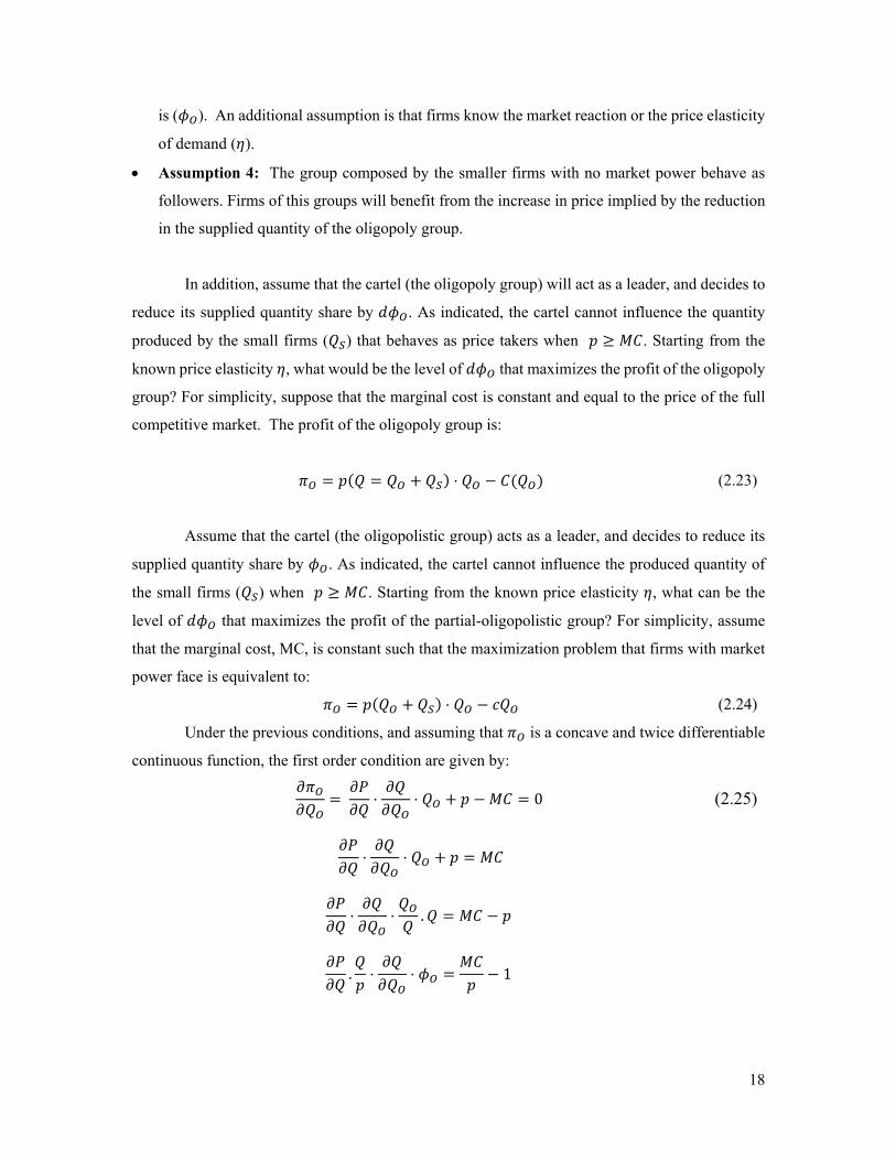
is ( ). An additional assumption is that firms know the market reaction or the price elasticity

of demand ( ).

Assumption 4: The group composed by the smaller firms with no market power behave as

followers. Firms of this groups will benefit from the increase in price implied by the reduction

in the supplied quantity of the oligopoly group.

In addition, assume that the cartel (the oligopoly group) will act as a leader, and decides to

reduce its supplied quantity share by . As indicated, the cartel cannot influence the quantity

produced by the small firms ( ) that behaves as price takers when . Starting from the

known price elasticity , what would be the level of that maximizes the profit of the oligopoly

group? For simplicity, suppose that the marginal cost is constant and equal to the price of the full

competitive market. The profit of the oligopoly group is:

⋅ (2.23)

Assume that the cartel (the oligopolistic group) acts as a leader, and decides to reduce its

supplied quantity share by . As indicated, the cartel cannot influence the produced quantity of

the small firms ( ) when . Starting from the known price elasticity , what can be the

level of that maximizes the profit of the partial-oligopolistic group? For simplicity, assume

that the marginal cost, MC, is constant such that the maximization problem that firms with market

power face is equivalent to:

⋅ (2.24)

Under the previous conditions, and assuming that is a concave and twice differentiable

continuous function, the first order condition are given by:

⋅ ⋅ 0 (2.25)

⋅ ⋅

⋅ ⋅ .

. ⋅ ⋅ 1

 

19  

1⋅ 1 ⋅ 1

1⋅ 1

1

1⋅ (2.26)

This formula reproduces some familiar results. For instance, it follows from formula (2.26)

that if → 0, then , the classical result in competitive markets. Also, this formula could

be used to infer some information on the proportion of increase in the price implied by the market

concentration.

Going from the competitive market outcome, , to the partial collusive

oligopoly, , implies a proportional price increase of:

11 ⋅

⋅1

11

1

11

1 1

1

1

(2.28)

Empirically, it is assumed that the observed market share of the oligopoly group with PCO

( ) is lower than in the competitive market ( ). Precisely, the observed market share is:

∗ ⋅1 ∗ ⋅

Thus, we have:

⋅ 1 ∗ ⋅ ∗ ⋅

 

20  

In general, while in the monopoly case a positive change in price implies that: 1, in

the PCO model the constraint becomes . The PCO model can justify existence of the

market power even if the elasticity is lower than one, and this what makes such a model attractive.

Based on 2.5 and 2.28, we find the following result:

⋅ ⋅11 ∗

⋅ ⋅11 ∗

∗ ⋅1

1 ∗ ⋅

∗ ⋅ ∗ ⋅

∗ ⋅∗ ⋅

(2.29)

 

1∗

∗ ⋅

∗ ∗ ⋅  

∗1 (2.30)

Next, the User Manual reports two illustrative examples for the two suggested methods of

the PCO model. Let 0.8, =0.20, the observed exchanged total quantity is 1000. For the

monopoly example, we assume that the elasticity is -1.2. The following table gives the results of

the two examples.

Competitive market PCO market

∗ 1.5/ 1 0.25 ∗ 2.5 =-0.9231

∗ / 1 1

1.5

1.00 11 /

1.25

1.00 1.00

 

21  

0.7

700

_ = 1 0.9231 ∗ 0.25 ∗ _

_ 390

0.3

_ 300

Profit = (1-1)*390=0 Profit = (1.25-1)* 300≈75

Competitive market MONOPOLY market

∗ 1.2/ 1 5 ∗ 2.2 =-.1

∗ / 1 1

1.2

1.00 11 1/

6

1.00 1.00

_ 1000

_ = 1 .1 ∗ 5 ∗ _

_ 2000

Profit = (1-1)*2000=0 Profit = (6-1)* 1000≈5000

The suggested PCO model offers three main advantages:

i. The User not need to know the exact number of firms, but can model the market using

information on the share of the largest firms.

ii. This market structure requires moderate information to assess the impact of market

concentration on prices. Mainly, it requires the elasticity of demand and the market

share of the oligopoly group.

iii. The suggested model mimics the real life and where we observe that small and large

firms realize some profits.

d. Partial market adjustment The three previous subsections discuss cases of complete movements from a market

concentration situation to a perfective competitive market, or vice versa. However, it may be

helpful to cover the case of a partial or stepwise movement. For instance, suppose a situation when

starting from a given number of oligopoly firms, the user is interested in assessing the impact of a

discrete increase in the number of firms. In addition, notice that the monopoly model is similar to

 

22  

the PCO model when the oligopoly market size is equal to 100%. In general, for the monopoly and

PCO models, it is possible to assume that a partial movement implies a decrease in the market size

from to .

Starting from the equation (2.30), is possible to show that:

∗ ∙ 1

Then:

Finally, for the case of oligopoly with the Nash equilibrium:

1 ∗ 1

Such that:

11 ∙

2.3 Price changes and the household well-being

This User Manual focuses in estimating the welfare impacts derived from changes in prices

following the tradition of indirect welfare measurement. The essential empirical problem that this

section of the User Manual discusses is how to measure welfare changes when the price of at least

one of the goods considered changes and if utility, demand or both are unknown (Abdelkrim and

Verme, 2016). There are three alternative money-metric well-being measurements in the mcwel

Stata module:22 the Laspeyres measure, the equivalent variation measurement and the compensated

variation measurement. This section briefly discusses the characteristics of each of the

measurements.

The indirect utility depends on the level of income and that of prices of goods and services.

According to King (1983), the equivalent income is a level of income for which one can keep the

level of utility unchanged after the change in prices. Formally, if the indirect-utility function is

denoted by V, we can write:

                                                            22 Hicks (1942) discusses five common measures of welfare changes: (i) Consumer’s surplus variation, (ii) compensating variation, (iii) equivalent variation, (iv) Laspeyres variation, and (v) Paasche variation. For a recent discussion of alternative welfare measures see Abdelkrim and Verme (2016).

 

23  

; ≡ ;m

where and denote the vectors of prices in and periods respectively and tem denotes the

equivalent income.

; ; m

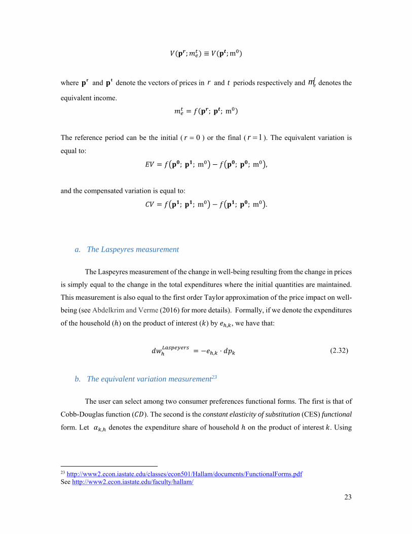
The reference period can be the initial ( ) or the final ( ). The equivalent variation is

equal to:

; ; m ; ; m ,

and the compensated variation is equal to:

; ; m ; ; m .

a. The Laspeyres measurement

The Laspeyres measurement of the change in well-being resulting from the change in prices

is simply equal to the change in the total expenditures where the initial quantities are maintained.

This measurement is also equal to the first order Taylor approximation of the price impact on well-

being (see Abdelkrim and Verme (2016) for more details). Formally, if we denote the expenditures

of the household ( ) on the product of interest ( ) by , , we have that:

, ⋅ (2.32)

b. The equivalent variation measurement23

The user can select among two consumer preferences functional forms. The first is that of

Cobb-Douglas function ( ). The second is the constant elasticity of substitution (CES) functional

form. Let , denotes the expenditure share of household on the product of interest . Using

                                                            23 http://www2.econ.iastate.edu/classes/econ501/Hallam/documents/FunctionalForms.pdf See http://www2.econ.iastate.edu/faculty/hallam/

rp tp r t

0r 1r

 

24  

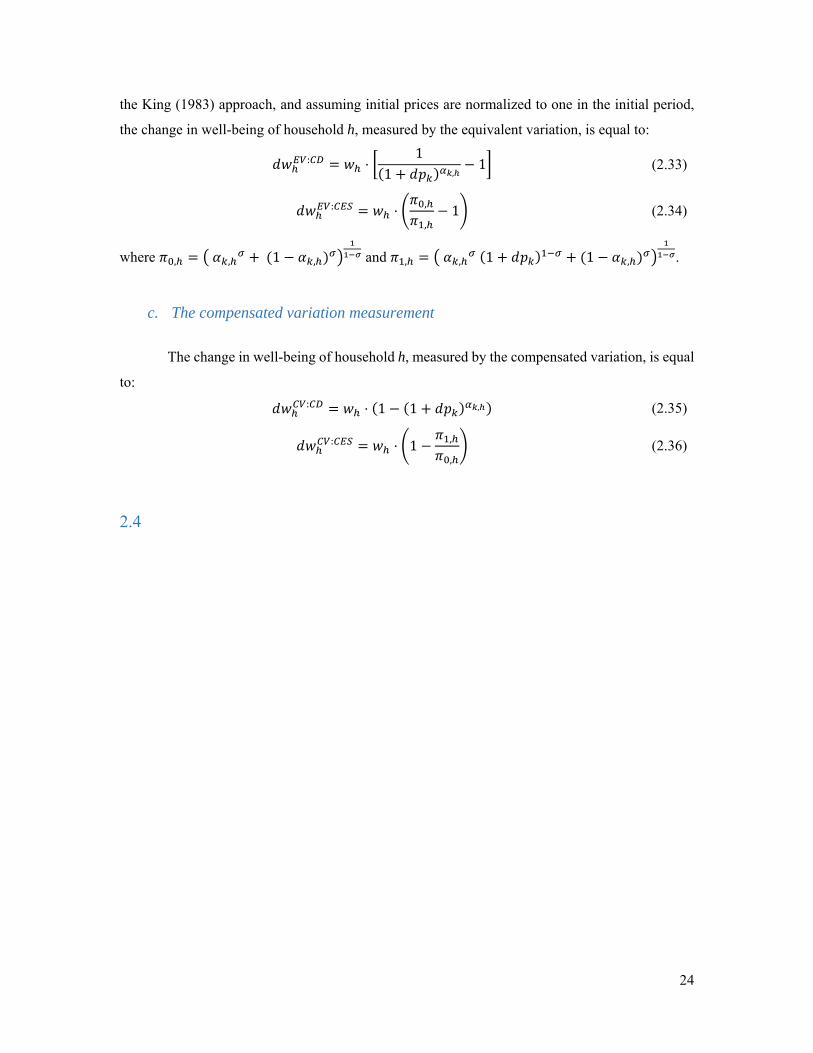
the King (1983) approach, and assuming initial prices are normalized to one in the initial period,

the change in well-being of household h, measured by the equivalent variation, is equal to:

: ⋅1

1 ,1 (2.33)

: ⋅ ,

,1 (2.34)

where , , 1 , and , , 1 1 , .

c. The compensated variation measurement

The change in well-being of household h, measured by the compensated variation, is equal

to:

: ⋅ 1 1 , (2.35)

: ⋅ 1 ,

, (2.36)

2.4

 

25  

3. The WELCOM Stata Package

The fourth section of this User Manual discusses the installation, preparation of data and

alternative methods of analysis available in mcwel tool to estimate the impacts of competition

policy reforms in welfare.

3.1 Installation

To install WELCOM execute the following commands in the Stata command line. Note

that it is possible to either copy and paste these lines directly in the command window or in the

dofile editor preferred by the User:

Commands 01

set more off

net from http://dasp.ecn.ulaval.ca/welcom/Installer

net install welcom, force

cap addmimenu profile.do _ welcom_menu

_ welcom_menu

Note: The Stata command lines in the chart Commands 01 tries to add the file profile.do

automatically or add the command _welcom_menu in this profile file, if the latter already exists.

However, if the previous commands do not function, the User needs to manually copy and paste

the profile.do file in the following locations (based on the operating system of the computer):

a. Windows OS system: copy the file in c:/ado/personal/

b. Macintosh system: copy the file in one of the Stata system directories. To find these

directories, type the command sysdir.

Once the previous steps were executed, the User should close all Stata sessions and restart

the program. After opening a new window, the User should be able to go to the menu bar in Stata,

click on the User option, choose the WELCOM package, select the Market concentration option

and launch the mcwel tool by clicking on Market concentration and well-being:

 

26  

Point and click 01

User > WELCOM > Market concentration > Market concentration and well-being

After selecting the “Market and well-being” option, a window with the main user interface

of the mcwel module will open and the User can start interacting with the program:

Figure 4.1: Main tab in mcwel module interface

 

27  

Note that the WELCOM package also provides the option of “WELCOM package

manager” to manage updates in the tool, read the reference material or visit the WELCOM

website24 as shown in Figure 3.2 below:

Point and click 02

User > WELCOM > WELCOM Package Manager

The following window corresponds to the user interface of the WELCOM: Package

Manager, showing alternatives to manage the version of the WELCOM Package and of the mcwel

Stata tool:

Figure 3.2: WELCOM: Package Manage Window

                                                            24 http://WELCOM

 

28  

After the User executes the commands in the table Commands 01 and launches the mcwel

tool following the instructions in Point and click 01, the tool is ready for use. The next section will

discuss in more detail the user interphase of the mcwel module for Stata.

3.2 The WELCOM package for Stata

The WELCOM package for Stata and was designed to assess the impact of changes in

consumer prices resulting from policy interventions to strengthen competition in specific markets

relying on the alternative theoretical models discussed in Section 3.2 of this User Manual. The

current version of the tool is flexible enough to accommodate three alternative market structures

and firms’ competitive behavior:

Monopoly: probably the simplest situation, when a single firm or a group of collusive firms

acting as a single supplier have market power on the supply side.

Oligopoly: in this scenario, a small number of firms with market power control the supply side

and compete generating a Cournot-Nash equilibrium.

Partial collusive oligopoly: a small number of firms with market power control a given share

of the market supply side and several smaller firms with no market power behave as price

takers.

The empirical analysis produced by the tool is based on micro-economic models where the

household is the unit of reference. One of the advantages of the tool is that it has mild minimum

data requirements that allow the User to run ex-ante analysis of policies aimed at strengthening

competition. The data requirements of the tool include:

A representative sample of the population (i.e., a consumption survey).

Information on total household expenditures (i.e., a variable representing a consumption

aggregate).

Data on household expenditures on the product of interest where we observe the market

concentration or expect a competition policy reform.

Information on one of the following parameters of the model (market structure), based on the

characteristics of the industry under study:

Monopoly: demand price elasticity.

Oligopoly: number of firms in the market and demand price elasticity.

Partial collusive oligopoly: market share of the firms colluding and the demand price

elasticity they face.

 

29  

Note that the data requirements of WELCOM can typically be met with data from two

alternative sources. On one hand, a household survey with a consumption module should provide

enough information on total consumption and expenditure in the type of good of interest. On the

other hand, basic information on the characteristics of the market and market structure can be

obtained from industry reports (such as the number of firms and market shares), studies from

government agencies (market shares, elastic of demand, collusive agreements) and firms or

industry surveys (number of firms, market shares), among others.

The rest of this section of the User Manual presents the different elements and features of

the tool in five parts:

a. Preparing the dataset

b. Launch the dialog box

c. Load the key variables

d. The “Main” tab

e. The “Items” tab

f. Select options to produce tables

g. Select options to produce graphs

h. The “if/in” tab

a. Preparing the dataset

Prior to launching the dialog box it is necessary to load in the memory of Stata a database

including variables with the relevant information on consumption in the format required by the tool

as well as additional characteristics on the market structure for the alternative options that the user

would like to estimate.25 The tool requires information on the following dimensions of household

characteristics and poverty measurement in the market:

Expenditure per capita in the product of interest: to analyze the effects of competition

policy interventions, the dataset available should include information on expenditure per

capita in the good or service where a firm or group of firms have market power or where a

competition policy reform is expected to have impact.

                                                            25 Please notice that if the database of interest already includes all the necessary variables to use the mcwel command it can be directly load to memory from the mc dialog box.

 

30  

Per capita expenditures: since the estimation of the effects of the competition policies

rely on a relative incidence analysis, information regarding the overall level of expenditure

per capita is also required.

Household size: the tool also requires to identify a variable capturing the size of the

household.

Poverty line: a variable representing the relevant poverty line (alternatively, other line

such as extreme poverty, vulnerability or middle class could be used) is necessary to assess

the effects of the intervention on poverty.26

In Figure 3.3. the User Manual shows a simple example of the kind of data on consumption

that the tool requires:

Figure 3.3: Data Requirements

In addition, the mcwel command allows to include the sample weights of the survey and,

ideally, additional variables indicating the Primary Sampling Unit (PSU) and Strata. Moreover, the

tool also allows the user to include a variable with information on the finite sample population

                                                            26 The current version of the tool expects that the three monetary variables (expenditure in the relevant good, total expenditure and poverty line) are expressed in comparative terms, for instance in current local currency units or in real terms using the same base year.

 

31  

correction. However, if no information on the sample design of the survey is entered (the sampling

design is not initialized), the simple random sampling is used by default.

Moreover, by default the tool will analyze the impacts of the policies by expenditure

quintiles, however we may want to include a variable capturing a different disaggregation such as

income deciles (to perform a relative incidence analysis by income decile), the urban/rural divide,

bottom 40 and top 60, or an indicator of ethnicity, among others.

b. Launch the dialog box

Once the relevant database is loaded in the memory of the Stata program, the dialog box

of the tool enables the User to interact with the tool and identify the variables with the required

information on household consumption, as well as to select the appropriate models—and their

parameters—for the alternative market structures and estimations. Thus, after the User loaded to

memory the database with the relevant variables for the analysis, she can launch the dialog box

following the steps discussed in the following Point and click 03 table:

Point and click 03

User > WELCOM > Market concentration > Market concentration and well-being

Once the tool in Stata is launched the user interface will show a window with the “Main”

tab, where the variables and parameters of the models to be analyzed can be selected. In addition,

there is a second tab labeled “Items” where the User can indicate the markets or products under

analysis. A third tab is optional and called “Table Options” to select the tables to be produced as

 

32  

well as the location to save an Excel file with such tables. The “Graph Options” tab allows the User

to choose alternative options to produce graphs. Finally, the “if/in” allows the User to select a

subsample of the observations for the analysis. The “Figure 3.4: Tabs in the mcwel window” shows

the location and main view of each of the tabs available in WELCOM.

Figure 3.4: Tabs in the main window

In the rest of this section, the User Manual will discuss the different elements that

compound each of the tabs available in the dialogue box of the tool.

c. The “Main” tab  

The “Main” tab of the tool is organized in seven sections, as indicated by the red circles in

Figure 3.5, each associated to a different element of the data available, characteristics of the sample

design, market structure and survey design, among others.

In addition, the “Main” tab also includes a box at the bottom right that the User can check

if she wants to “Generate the variable for the impact on well-being”, in case the User wants to

generate a new variable in Stata to store the results of the analysis of the impacts of competition

policy reforms.

 

33  

Figure 3.5: Elements of the Main Tab Window

In the rest of this section each of the options in the seven section of the Main tab showed

in Figure 3.5 will be discussed in detail:

Dialog box inputs

General information on the sampled households

Group variable

Prices and well-being model

Estimated impact

Parameters of inequality indices

The Dialog box inputs 

This is to load and save the dialog box information. The box enables the user to load

information already saved into the WELCOM window, or to save the information inserted in the

dialog box in a file to be stored for future simulations. This information is stored in text files with

 

34  

the extension *.mcw. You can test this feature by uploading the file “mcwel_example.mcw”

provided with the toolkit. Note that you can load the file from one directory (“Load the Inputs”)

and save it in a different directory with a different name (“Save the Inputs”).

Point and click 04

User > WELCOM > Market concentration > Market concentration and well-being > Main > Dialog box inputs

General information on the sampled households 

 

The box “General information on sampled households” is located at the top left of the

window. This box includes 4 options to select the relevant variable from the database in memory

using a dropdown menu such as the one showed in Point and click 04 chart. At a minimum, the

tool requires the user to introduce information about the following three variables of interest:

i. Per capita expenditures: continuous numerical variable with monetary values.

ii. The household size: integer variable.

iii. The poverty line: continuous numerical variable with monetary values.

 

35  

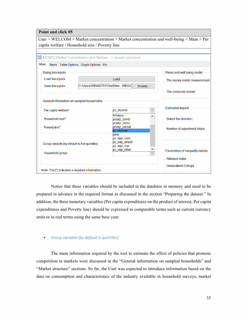
Point and click 05

User > WELCOM > Market concentration > Market concentration and well-being > Main > Per capita welfare / Household size / Poverty line

Notice that these variables should be included in the database in memory and need to be

prepared in advance in the required format as discussed in the section “Preparing the dataset.” In

addition, the three monetary variables (Per capita expenditures on the product of interest, Per capita

expenditures and Poverty line) should be expressed in comparable terms such as current currency

units or in real terms using the same base year.

Group variable (by default is quintiles) 

The main information required by the tool to estimate the effect of policies that promote

competition in markets were discussed in the “General information on sampled households” and

“Market structure” sections. So far, the User was expected to introduce information based on the

data on consumption and characteristics of the industry available in household surveys, market

 

36  

studies, firm surveys or other sources. Now, the User is expected to introduce information on the

way she wants the data to be analyzed and the estimates and results to be presented.

The box “Group variable” enables the User to select a population group variable in a

dropdown menu from the database in memory or by directly introducing the number of groups to

classify the households given their expenditure levels, as shown in the Point and click 06 chart.

Point and click 06

User > WELCOM > Market concentration > Market concentration and well-being > Main > Household group

Notice that, in contrast with the previous boxes where the User had to either select an

alternative or introduce a value, now she can either choose to select a variable or directly introduce

an integer value representing the number of groups required. If the User decides to group the

estimates using a variable, the results could show the differences by socio-demographic group such

as gender or urban-rural area of residence. In contrast, if the user indicates an integer such as 10 in

the “Household group” option, the population is organized by decile groups based on their level of

expenditure. If the “Household group” option is left empty, then the results are shown organized

by expenditure quintiles by default.

 

37  

Price and well‐being model 

Once the data on consumption, the parameters on the characteristics of the market and the

organization of the results is selected, the User needs to decide the type of measurement to use to

estimate the impacts of the policy fostering competition. More precisely, this implies choosing the

main approach to be adopted to assess the impact of price change on well-being. The user can select

among the three following alternative measurements (see the Section 3.3 for more details on the

characteristics of these measures).

The Laspeyres measurement (linear approximation).

The equivalent variation measurement.

The compensated variation measurement.

Point and click 07

User > WELCOM > Market concentration > Market concentration and well-being > Main > Select the structure > Prices and well-being model

Estimated impact 

So far, this User Manual has implicitly assumed that the base scenario under analysis is

one where a concentrated market exists, such that the authorities responsible of policy design have

identified the presence of market power and are planning to implement a policy to promote

competition in the market. Therefore, the analysis of the effects of the policy implicitly assume

moving from an industry where a group of firms exploit their market power, to a competitive market

 

38  

where firms are not able to extract market power rents and charge prices according to their marginal

costs.

Point and click 08

User > WELCOM > Market concentration > Market concentration and well-being > Main > Estimated impact

However, the tool is flexible enough to accommodate the analysis of policies aimed at

fostering competition in the market (e.g., by selecting the “Concentrate to Competitive Market”

option in the “Select the direction” box) as well as the opposite scenario, where a policy is expected

to somehow reduce competition in the market (e.g., limit imports, setting price ceilings, creating

artificial monopolies, etc) and the User needs to assess the impact on welfare of moving from a

competitive market to a more concentrated one.

To switch between the base scenarios that the User wants to run for the analysis, she can

go to the “Estimated Impact” box and follow the indications in the Point and click 08 chart below.

Notice that as the User change the base scenario, the interpretation of the results should also be

adjusted to reflect the relevant conditions.

In addition to estimating the impact of moving from the initial to the final state (for instance

from the concentrated market to the competitive market), the module can estimate the intermediate

states of the partial movements toward the final state. This is can be achieved by indicating the

number of steps of adjustments. For instance, assume that we have a case of a PCO model for which

 

39  

the market size of the oligopoly firms is equal to 60%. If the selected number of adjustment is zero,

then the tool estimates directly the impact of a full impact. If the number of steps is one, then the

impact is estimated from a change of the market change from 60% to 30% and then from 60% to

0%. As a general rule, if we denote the initial market share by and the number of steps by ,

then, the intermediate steps are: → ∈ 1; . The monopoly is a special case when

100%.

Now, assume the case of the oligopoly market structure which a Nash equilibrium that

depends on the number of firms. For instance, if the initial number of firms is 4, and the

number of steps is three, the intermediate steps are: for 6, 8 12. As a general rule, when

the number of steps is , then, the intermediate steps are:

: → ∗ 1.5// Step 2 to s: → ∗ ∈ 2; .

As an additional example, in table ##, we present some displayed results for the case of

two product items (Combustible and Communication). In this case, the indicated number of steps

is 3. For the combustible item, the initial marker size is 42.31%. The step1 is by moving toward the

competitive market by a decline is the size from the 42.31 to 42.31/2, the step 2 is a decline in size

until 42.31/3 and the step 3 is a decline until 42.31/4=10.57%. For the Communication item, the

initial number of the oligopoly firms is 8, in the step 1 it increases by 50% to 12, and then it doubles

in step 2 and triple in step 3.

The number of adjustment steps and results

The user can select another number of steps of adjustments, and this to have more refined

results if needed.

Parameters of inequality indices 

Market size (in%)

Elasticity Price # of firms Elasticity Price

Concentrated_Market 42.3100 -0.9040 1.8798 8.0000 -0.6430 1.1628

Step___1 21.1550 -0.6210 1.5167 12.0000 -0.5821 1.1252

Step___2 14.1033 -0.5266 1.3658 16.0000 -0.5517 1.1018

Step___3 10.5775 -0.4794 1.2831 24.0000 -0.5213 1.0740

Competitive__Market 0.0000 -0.3379 1.0000 . -0.4604 1.0000

Table 1.1: Models and parameters

Combustible Communication

 

40  

In the “Parameters of inequality indices” the tool offers the option to select some of the

parameters necessary to estimate the two alternative inequality indices:

a. The Atkinson index

b. The Generalized Entropy

Point and click 09

User > WELCOM > Market concentration > Market concentration and well-being>Survey settings

Survey settings 

Notice that to use the options for survey settings, the User needs to prepare the variables

associated with the different dimensions of the survey design before launching tool. These settings

include information on the sampling weights, sampling design, adjustment for finite population,

among others. This can be done with the command “svyset” in Stata or using the button “Survey

Settings…” located in the bottom right-hand corner of the “Main” tab, as shown in the Point and

click 08 chart.

 

41  

Point and click 10

User > WELCOM > Market concentration > Market concentration and well-being>Survey settings

For more information on the alternative survey settings available in the tool, see the Stata

Reference Manual on Survey Data.

 

42  

Figure 3.6: Survey Settings Options in the tool

d. The “Items” tab

Among the main improvements in the version 2.0 is the possibility of estimating the

impacts of different market concentrations. The tab “Items” enables to indicate the number or

products of interest with concentration markets, as well we, the market structure of each

product/item. While the options in the “Main” tab generally rely on information from a household

or consumer survey, the information for the “Items” tab comes from studies on the organization of

the industry or market under study as well as from firm surveys or analysis on competition

conditions from the competition market authorities (CMA).

The user can choose from 1 to 10 items. For each item, the user can indicate:

The short name of the item or the product.

The variable name of the expenditures per capita.

The market structure: The tool needs information on the structure of the supply side of the

industry, i.e. how many firms or suppliers are and how do they interact in the market. In

addition, each model of market structure requires a different set of parameters that the User

requires to feed into the mcwel tool. For instance, while the Monopoly structure only requires

information on the elasticity of the demand, the Oligopoly: Nash Equilibrium needs in addition

to the demand elasticity, information on the initial number of firms in the market. Following

the instructions in the chart Point and click 05, the user can select among three alternative

structures and the required industry parameters:

 

43  

a. Monopoly: The User only needs to provide the value of the price elasticity of the demand.

Notice that this elasticity is typically a negative parameter in the range (-1,0) since by

theory the monopolist optimizes by producing in the elastic segment of the demand curve.

b. Oligopoly-Nash equilibrium: Under this type of market structure, the User must provide

information on the elasticity of demand faced by the firms, as well as on the number of

firms in the oligopolistic market.

c. Partial collusive oligopoly: In this scenario, the User must provide the value of the price

elasticity of demand as well as the observed market share of the oligopolistic group.

The non-compensated elasticity.

The number of firms (model: Oligopoly: Nash equilibrium).

The market size of the oligopoly group (model: PCO).

Point and click 11

User > WELCOM > Market concentration > Market concentration and well-being > Items > Number of firms

 

44  

It must be noted that one of the caveats of the analysis currently available in the tool is that

the welfare outcomes of the alternative market structures are compared against a perfect

competition counterfactual. This implies that the tool assumes, for instance, that after implementing

a policy reform aimed at eliminating a monopoly in a market, this market will become perfectly

competitive, assumption that might be problematic in some circumstances.

e. The “Table Options” tab

This tab allows the user to select the tables’ options. The default option when you do not select the

tables and override options is the production of all tables.

Tables: Select the tables to be produced 

In case the user wishes to have only a selected number of tables the code of these tables can be

indicated in the box. The list of codes with the titles of the tables can be seen by clicking on the

question mark button “?”. For example, you can type “11 23” to produce tables 1.2 and 2.3 only

(no commas, one space between numbers).

Excel file: Produce an Excel file of results 

This box allows the user to define the Excel file where all tables should be stored. The user can

select an existing file to override or create a new file. The user can either specify the name of the

file or not. In the case of an existing file, the user should make sure that this file is closed when the

program is launched, otherwise an error message will appear.

 

45  

Point and click 12

User > WELCOM > Market concentration > Market concentration and well-being > Table Options

f. The “Graph Options” tab

The tab on the Graph Options allows the User to decide if she wants the tool to produce

graphs with the estimated impacts of the analysis of the policy interventions aimed at foster

competition, and what are the parameters and characteristics of the graphs. To access the “Graph

Options” tab, the User should follow the indications in the Point and click 10 box. The main three

options available allow to select the graphs to be produced, choose the folder to save such graphs

and select among alternative graph options.

Graphs: Select the graphs to be produced 

This option allows the User to save only selected graphs by indicating the code of each

graph. The list of codes with the titles of the graphs can be seen by clicking on the question mark

button “?”. For example, if the user wishes to produce only Graphs 1, 2 and 4, the user will simply

type “1 2 4” (no commas, one space between numbers).

 

46  

Select the folder of graph results 

This option allows the user to select the directory where the saved graphs should be stored.

Note that all graph files are saved in three formats: .gph. .pdf and .wmf. will save a folder with the

name “Graphs” in the directory selected.

Graph options 

For each graph, the user can select options regarding the y-axis scale (min and max) and

other two-way graphs options as indicated in the Stata graph help files. For example, users may

want to limit the range of the graphs to a specific interval like between 10 and 80. This can be done

by indicating min and max values. Or users may want to omit titles of the graphs to add these titles

separately in the report. This can be done by adding the Stata graph option “title (“”)”. Note that

each of the displayed graphs is automatically saved in three format in a the previously indicated

folder (“Graph”). The three format the saved graphs are: (i) *.gph; (ii) *.wmf; and (iii) *.pdf.

 

Point and click 13

User > WELCOM > Market concentration > Market concentration and >Graph options

g. The “if/in” tab

The “in/in” tab includes a single command box to select a relevant subsample from the

database on memory to perform the analysis.

 

47  

Restrict observations  

Note that, as shown by the Point and click 09 box below, the mcwel tool offers two main

ways to restrict the observations to a smaller subsample. The first alternative is to select

observations conditional on a specific if expression or criteria. The second alternative implies

restricting the analysis to a predetermined range of observations.

Point and click 14

User > WELCOM > Market concentration > Market concentration and well-being>if/in

3.3 The mcwel outputs

After launching the computation, a series of results (tables and figures) are displayed. The

main results tables provided are:

a. The estimated market parameters

In table 1, the price change, the adjusted elasticity and the rest of used or estimated

parameters of the market structure are reported.

 

48  

b. The descriptive statistics on household expenditures

In table 2, the average per capita to expenditures and that on the product of interest are

reported for each population group. Also, it is displayed the expenditure shares.

c. The impact of the market concentration on household well-being

In table 3, the price change implied by the moving from a market without concentration to

that with concentration is reported. In addition, table 3 reports the average impact of the price

change on household well-being, and this by population groups.

d. The impact of the market concentration on poverty

In table 4, the three popular poverty indices are reported for the cases of with and without

market concentration. Also, the impact of the market concentration on poverty is reported.

e. The impact of the market concentration on inequality:

In table 5, four inequality indices are reported for the cases of with and without market

concentration. Also, the impact of the market concentration on the inequality is reported. The

inequality indices are:

The Gini index;

The Atkinson index;

The generalized entropy index;

The Quantiles ratio index (Q(p=0.1)/Q(p=0.9)).

Note: The full information on the sampling design of the survey is used to assess the

standard error of the different statistics.

The Figure results are:

The expenditures share on the product of interest, per the well-being percentile;

The per capita impact on well-being according to the well-being percentile;

The Lorenz curve of well-being and the concentration curve of the product of interest.

 

49  

3.4 Examples of WELCOM

Example 01:

Step 1: Be sure that you have installed the WELCOM

Step 2: load the zipped folder:

http://dasp.ecn.ulaval.ca/WELCOM/examples/mcwel_examples.rar

Step 3: Unzip the loaded folder in a given folder location: for instance c:/PDATA/WELCOM2/

Step 4: Open the dialog box (type: db mcwel);

Step 5: Load the file mcwel_example_01.mcw. This step will initialize the information in the

dialog box

Step 6: Click on the button submit.

In this first example, we would like to produce the tables 1.1 and 1.2, as well as the figure 01. We

have three items of interest, and their three corresponding market structures are already indicated

in the TAB items of the dialog box. As we can remark in the box estimated impact, we would like

to estimate the impact of moving from the concentrated market to the competitive market.

Further, we would like to estimate the impacts of a six partial moving toward the competitive

markets.

 

50  

For instance, for the combustible item, we have initially a PCO market structure, and where the

market share of the oligopoly firms is 42.31 %. In the first step of the adjustment toward the

competitive market, the market share is reduced, by the half, and then by two thirds and so on.

Table 01 also shows the corresponding elasticities and prices.

Competitive Market 0.000 -0.4305 1.000000 Step : 6 4.959 -0.5014 1.109745 Step : 5 5.785 -0.5132 1.127035 Step : 4 6.942 -0.5298 1.150793 Step : 3 8.677 -0.5546 1.185481 Step : 2 11.570 -0.5960 1.240897 Step : 1 17.355 -0.6787 1.343533 Concentrated Market 34.710 -0.9270 1.598550 Step Market size (in%) Elasticity Price Item: Cereals Market type : Partial Collusive Oligopoly Competitive Market . -0.4604 1.000000 Step : 6 48.000 -0.4909 1.040714 Step : 5 40.000 -0.4970 1.047897 Step : 4 32.000 -0.5061 1.058158 Step : 3 24.000 -0.5213 1.074013 Step : 2 16.000 -0.5517 1.101755 Step : 1 12.000 -0.5821 1.125223 Concentrated Market 8.000 -0.6430 1.162760 Step # of firms Elasticity Price Item: Communication Market type : Oligopoly: Nash Equilibrium Competitive Market 0.000 -0.3379 1.000000 Step : 6 6.044 -0.4188 1.168670 Step : 5 7.052 -0.4323 1.194930 Step : 4 8.462 -0.4511 1.230875 Step : 3 10.578 -0.4794 1.283072 Step : 2 14.103 -0.5266 1.365767 Step : 1 21.155 -0.6210 1.516716 Concentrated Market 42.310 -0.9040 1.879809 Step Market size (in%) Elasticity Price Item: Combustible Market type : Partial Collusive Oligopoly Table 1.1: Models and parameters

 

51  

Table 02 gives some descriptive statistics on the population and the expenditures

Figure 01 gives more refined results similar to those of table 1.1:

Figure 1: The mcwel table outputs

Example 02:

Step 5: Load the file mcwel_example_02.mcw.  

Step 6: Click on the button submit.

Total 119906312 31671002 3.79 419560521728 3499.07 13247.47 Quintile 5 23969206 8784954 2.73 232294957056 9691.39 26442.37 Quintile 4 23986720 6734927 3.56 80423206912 3352.82 11941.21 Quintile 3 23982586 5894251 4.07 52534333440 2190.52 8912.81 Quintile 2 23958312 5402162 4.43 35458871296 1480.02 6563.83 Quintile 1 24009490 4854708 4.95 18849142784 785.07 3882.65 size per capita per household Groups Population Number of households Household Total expenditures Total expenditures Total expenditures Table 1.2: Population and expenditures (in currency)

11.

21.

41.

61.

8P

rice

(com

petit

ive

mar

ket =

1)

11.

051.

11.

151.

2P

rice

(com

petit

ive

mar

ket =

1)

11.

21.

41.

6P

rice

(com

petit

ive

mar

ket

= 1

)

 

52  

This example is similar to the first, but in this case the number of steps of adjustment are two and

we produce all of the tables and figures.

The mcwel module estimates the different statistics for each step of adjustment. For instance, for

the impact on the poverty headcount, the first table shows the level of poverty with the concentrated

market (53.352%), and then with only the partial adjustment of the combustible market (52.28).

The last line shows the impact of the partial adjustment in the three markets (51.43). The table 5.1

is reproduced for each adjustment step.

Competitive Market 0.000 -0.4305 1.000000 Step : 2 11.570 -0.5960 1.240897 Step : 1 17.355 -0.6787 1.343533 Concentrated Market 34.710 -0.9270 1.598550 Step Market size (in%) Elasticity Price Item: Cereals Market type : Partial Collusive Oligopoly Competitive Market . -0.4604 1.000000 Step : 2 16.000 -0.5517 1.101755 Step : 1 12.000 -0.5821 1.125223 Concentrated Market 8.000 -0.6430 1.162760 Step # of firms Elasticity Price Item: Communication Market type : Oligopoly: Nash Equilibrium Competitive Market 0.000 -0.3379 1.000000 Step : 2 14.103 -0.5266 1.365767 Step : 1 21.155 -0.6210 1.516716 Concentrated Market 42.310 -0.9040 1.879809 Step Market size (in%) Elasticity Price Item: Combustible Market type : Partial Collusive Oligopoly Table 1.1: Models and parameters

 

53  

 

For the poverty and inequality, the Figures 05 and 06 will show the partial impacts in a refined

way.

Competitive Market 49.057 -4.295 0.198 0.000 Cereals 51.557 -1.795 0.124 0.000 Communication 52.895 -0.457 0.073 0.000 Combustible 51.041 -2.311 0.147 0.000 Concentrated Market 53.352 . . . error Step Poverty level The change in poverty Standard P-Value Table 5.1: The market power and the poverty headcount || Concentrated to competitive: Full adjustement

Competitive Market 50.725 -2.627 0.156 0.000 Cereals 52.273 -1.079 0.097 0.000 Communication 53.219 -0.133 0.040 0.001 Combustible 51.923 -1.429 0.114 0.000 Concentrated Market 53.352 . . . error Step Poverty level The change in poverty Standard P-Value Table 5.1: The market power and the poverty headcount || Concentrated to competitive: Step 2

Competitive Market 51.435 -1.917 0.131 0.000 Cereals 52.566 -0.786 0.083 0.000 Communication 53.263 -0.089 0.027 0.001 Combustible 52.280 -1.072 0.101 0.000 Concentrated Market 53.352 . . . error Step Poverty level The change in poverty Standard P-Value Table 5.1: The market power and the poverty headcount || Concentrated to competitive: Step 1

 

54  

050

100

150

Num

ber

of fi

rms

010

2030

40M

arke

t siz

e (in

%)

0 5 10 15 20Steps

Steps and market power

Combustible

Communication

Cereals

.4969

.49695

.497

.49705

.4971

Ineq

ualit

y le

vel (

Gin

i)

0 10 20 30 40Market power (market size in %)

Combustible

.49699

.496992

.496994

.496996

Ineq

ualit

y le

vel (

Gin

i)

0 50 100 150Market power (Number of firms)

Communication

.488

.49

.492

.494

.496

.498

Ineq

ualit

y le

vel (

Gin

i)

0 10 20 30 40Market power (market size in %)

Cereals

.49

.492

.494

.496

.498

Pov

erty

leve

l (H

eadc

ount

)

0 5 10 15 20Steps

All items

Figure 06: Market power and inequality

050

100

150

Num

ber

of fi

rms

0

10

20

30

40

Mar

ket

size

(in

%)

0 5 10 15 20Steps

Steps and market power

Combustible

Communication

Cereals

.51

.515

.52

.525

.53

.535

Pov

erty

leve

l (H

eadc

ount

)

0 10 20 30 40Market power (market size in %)

Combustible

.529

.53

.531

.532

.533

.534

Pov

erty

leve

l (H

eadc

ount

)

0 50 100 150Market power (Number of firms)

Communication

.515

.52

.525

.53

.535

Pov

erty

leve

l (H

eadc

ount

)

0 10 20 30 40Market power (market size in %)

Cereals

.49

.5

.51

.52

.53

Pov

erty

leve

l (H

eadc

ount

)

0 5 10 15 20Steps

All items

Figure 05: Market power and poverty headcount

 

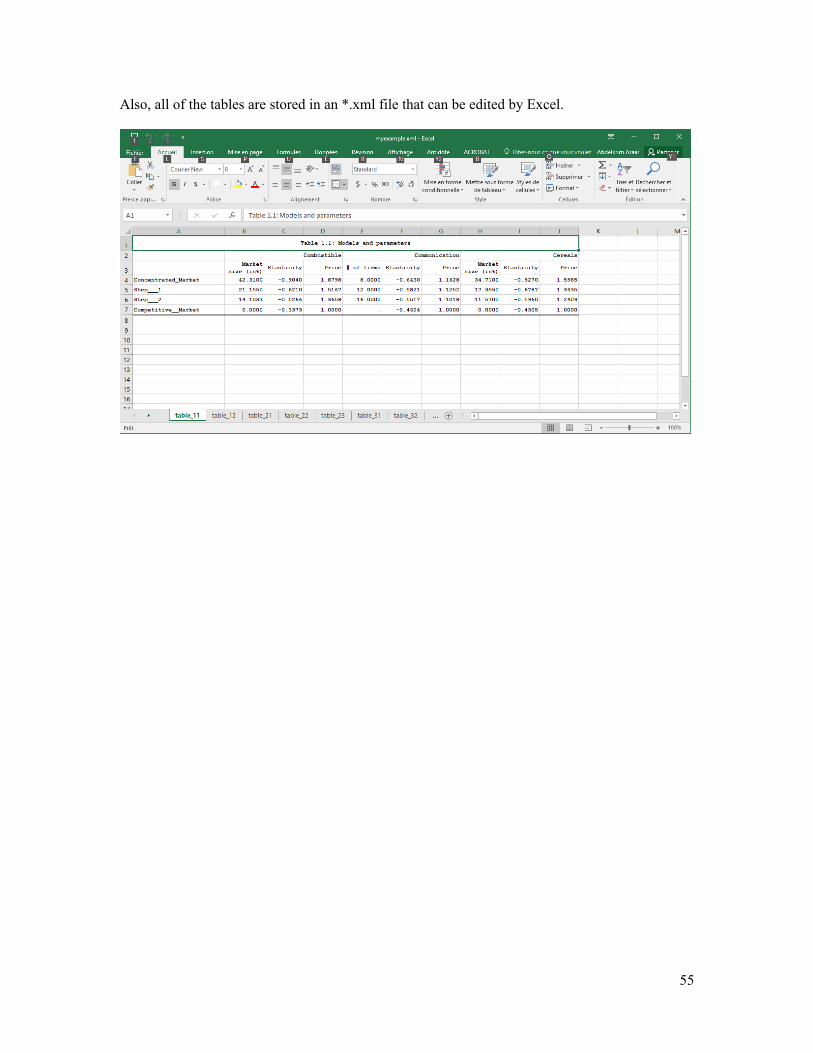
55  

Also, all of the tables are stored in an *.xml file that can be edited by Excel.

 

56  

References

Abdelkrim, A. and Verme, P. (2016). "Prices and welfare," Policy Research Working Paper

Series 7566, The World Bank.

Abdelkrim, A., Olivieri, S. and Rodriguez-Castelan, C. (2017). "Market Concentration and

Well-being: the Mexican Case," Working Paper.

Asker, J., Collard-Wexler, A., and De Loecker, J. (2017). “Market Power, Production (Mis)

Allocation and OPEC.” (No. w23801). National Bureau of Economic Research, NBER.

Bain, J. S. (1951). “The relation of profit rate to industry concentration: American

manufacturing,” Quarterly Journal of Economics, 65, 293–324.

Begazo, T. and Nyman, Sara (2016). “Competition and Poverty. How Competition Affects the

Distribution of Welfare.” Viewpoint 350, Trade and Competitiveness Global Practice, April

2016. The World Bank Group.

Bertrand, J. (1883). “Book review of theorie mathematique de la richesse sociale and of

recherches sur les principles mathematiques de la theorie des richesses.” Journal de Savants

67: 499–508.

Bridgman, B., Qi, S., & Schmitz Jr, J. A. (2015). “Cartels Destroy Productivity: Evidence from

the New Deal Sugar Manufacturing Cartel, 1934-74.” Federal Reserve Bank of Minneapolis

Staff Report, 519.

Buccirossi, P. (2008). “Handbook of Antitrust Economics,” The MIT Press. Cambridge,

Massachusetts.

Cournot A. (1838). “Researches on the Mathematical Principles of the Theory of Wealth.”

Fudenberg, D. and Tirole, J. (1991). “Game Theory.” The MIT Press. Cambridge,

Massachusetts.

Furman, J. (2016) "Beyond Antitrust: The Role of Competition Policy in Promoting Inclusive

Growth." (2016).

Gonzalez, A., Martinez-Licetti, M., and Goodwin, T. (2015). “From Tirole to the WBG Twin

Goals: Scaling up competition policies to reduce poverty and boost shared prosperity.” Web

blog post Private Sector Development Blog, July 10 of 2015. Web. August 30, 3017.

Harrington, J. E. (2017). “The Economics of Collusion and Competition Theory.” The MIT

Press, October 2017.

 

57  

Khan, L., & Vaheesan, S. (2017). “Market Power and Inequality: The Antitrust

Counterrevolution and Its Discontents.” Harv. L. & Pol'y Rev., 11, 235.

King, M. (1983): “Welfare Analysis of Tax Reforms Using Household Data,” Journal of Public

Economics, 21, 183–214.

Kreps, D. and Scheinkman, J. (1983). “Quantity Precommitment and Bertrand Competition

Yield Cournot Outcomes.” Bell Journal of Economics, 14:326-337.

Mas-Colell, A., Whinston, M. D., and Green, J. R. (1995). “Microeconomic Theory.” Oxford

University Press, Inc.

Olivieri, S., Radyakin, S., Kolenikov, S., Lokshin, M., Narayan, A., and Sanchez-Paramo, C.

(2014). “Simulating Distributional Impacts of Macro-Dynamics. Theory and Practical

Application,” Washington, DC: World Bank Group.

http://documents.worldbank.org/curated/en/240891468159907079/Simulating-distributional-

impacts-of-macro-dynamics-theory-and-practical-applications

Outreville, J. F. (2015). “The market structure performance relationship applied to the

Canadian wine industry.” Applied Economic Letters, Vol. 22, No. 18, pp. 1486-1492, 2015.

Perloff, J. M. (2013). “Microeconomics: Theory and Applications with Calculus, 3e.” Pearson,

2013.

Perry, M. K. (1989). “Vertical integration: Determinants and effects.” In Handbook of

Industrial Organization, Chapter 4, Elsevier, Volume 1, 1989, Pages 183-255, ISSN 1573-

448X, ISBN 9780444704344, https://doi.org/10.1016/S1573-448X(89)01007-1.

Rodriguez-Castelan, C. (2015). "The poverty effects of market concentration." Policy Research

Working Paper Series 7515, The World Bank.

Tirole, J. (1988). “The theory of industrial organization.” The MIT Press. Cambridge,

Massachusetts.

Tirole, J. (2015). “Market Failures and Public Policy.” American Economic Review 2015,

105(6):1665-1682.

Varian, H. (1992). “Microeconomic Analysis, Third Edition.” W.W. Norton & Company, Inc.

March 1992.

Varian, H. (2006). “Intermediate Microeconomics: A Modern Approach.” (7th ed.) W. W.

Norton & Company.

Viscusi, W. K., Vernon, J. M., and Harrington, J. E. (2005). “Economics of Regulation and

Antitrust, Fourth Edition.” The MIT Press. August 2005.