use of neural network/dynamic … of neural network/dynamic algorithms to predict bus ... to predict...
TRANSCRIPT
FHWA-NJ-2003-019
USE OF NEURAL NETWORK/DYNAMIC ALGORITHMS TO PREDICT BUS TRAVEL TIMES UNDER
CONGESTED CONDITIONS
Final Report November 2003
Submitted by
Dr. Steven I-Jy Chien, Associate Professor
Department of Civil and Environmental Engineering New Jersey Institute of Technology
Dr. Mei Chen, Assistant Professor
Department of Civil and Environmental Engineering University of Kentucky
Mr. Xiaobo Liu, Research Assistant
Interdisciplinary Program in Transportation New Jersey Institute of Technology
NJDOT Research Project Manager Edward Kondrath
DISCLAIMER STATEMENT
i
In cooperation with
New Jersey Department of Transportation
Division of Research and Technology and
U.S. Department of Transportation Federal Highway Administration

“The contents of this report reflects the views of the
author(s) who is (are) responsible for the facts and the
accuracy of the data represented herein. The contents do
not necessarily reflect the official views or policies of the
New Jersey Department of Transportation or the Federal
Highway Administration. This report does not constitute
a standard, specification, or regulation.
ii

iii
1. Report No. 2.Government Accession No. 3. Recipient’s Catalog No. FHWA-NJ-2003-019
Federal Highway Administration U.S. Department of Transportation Washington, D.C.
4. Title and Subtitle 5. Report Date November 2, 2003 6. Performing Organization Code
Use of neural network/dynamic algorithms to predict bus travel times under congested conditions
7. Author(s) 8. Performing Organization Report No. Steven I-Jy Chien, Mei Chen, Xiaobo Liu
9. Performing Organization Name and Address 10. Work Unit No.
11. Contract or Grant No.
Department of Civil and Environmental Engineering New Jersey Institute of Technology University Heights Newark, New Jersey 07102-1982
12. Sponsoring Agency Name and Address 13. Type of Report and Period Covered Final Report 14. Sponsoring Agency Code
New Jersey Department of Transportation Trenton, NJ
15. Supplementary Notes
16. Abstract Automatic Passenger Counter (APC) systems have been implemented in various public transit systems to obtain various types of real-time information such as vehicle locations, travel times, and occupancies. Such information has great potential as input data for a variety of applications including performance evaluation, operations management, and service planning. In this study, a dynamic model for predicting bus arrival times is developed using data collected by a real-world APC system. The model consists of two major elements. The first one is an artificial neural network model for predicting bus travel time between time points for a trip occurring at given time-of-day, day-of-week, and weather condition. The second one is a Kalman filter based dynamic algorithm to adjust the arrival time prediction using up-to-the-minute bus location (operational) information. Test runs show that the developed model is quite powerful in dealing with variations in bus arrival times along the service route. 17. Key Words 18. Distribution Statement Bus, Travel Time, Prediction, APC, ANN, Kalman filter, Schedule, Reliability, Data
No restriction. This document is available to the public through the National Technical Information Service, Springfield, Virginia 22161
19. Security Classif (of this report) 20. Security Classif. (of this page) 21. No of Pages 22. Price
None None 92
Form DOT F 1700.7 (8-69)

Acknowledgements
The authors acknowledge the support of the New Jersey Department of Transportation and the
National Center for Transportation and Industrial Productivity. The authors also thank Dr. Jerome
Lutin, Mr. Glenn Neuman, and Mr. James Kemp with the New Jersey Transit Corporation and Dr.
David Robinson with Rutgers the State University of New Jersey for providing valuable data used
in this study.
ii

TABLE OF CONTENTS
INTRODUCTION Overview 1 Background 1 Objective 3 Scope of Work and Organization 4 LITERATURE REVIEW Introduction 5 State of the Practice APTS 6 Applications 12 Prediction Algorithms 24 Media for Information Dissemination 27 DATA COLLECTION APC Data 33 GIS Data 33 Weather Data 37 Field Data 40 SELECTION OF STUDIED PATTERNS AND SOFTWARE Selection of the Study Patterns 42 Selection of Software 46 DATA PROCESSING Data Screening 47 Data Calculation 47 Data Interpolation 48 Summary 50 MODEL DEVELOPMENT Introduction 51 Artificial Neural Networks (ANNs) 51 Kalman Filtering Algorithm 65 PREDICTION EVALUATION AND ANALYSIS Performance of Artificial Neural Networks (ANNs) 68 Performance of the Neural/Dynamic (N/D) Model 74 CONCLUSIONS 87 REFERENCES 89
iii

LIST OF FIGURES
Figure 1 Configuration of the Studied Route and Its Adjacent Streets 35 Figure 2 Potential Stops on the Studied Route 36 Figure 3 Alignment of Bus Route 62 in GIS 36 Figure 4 NCDC Weather Observation Stations 37 Figure 5 Newark International Airport Station 38 Figure 6 Weather Information of the Selected Station 38 Figure 7 Time Period Selection for Querying Weather Information 39 Figure 8 Example of Collected Weather Information 39 Figure 9 Configuration of Bus Route 62 42 Figure 10 The Studied Patterns in GIS 45 Figure 11 MLP with One Hidden Layer 53 Figure 12 BPN Training Procedure 54 Figure 13 Sample Data File 57 Figure 14 Network Architecture of Model I 59 Figure 15 Learning Curves of Model I 60 Figure 16 Learning Curves of Model II 65 Figure 17 Learning Curves of Model III 63 Figure 18 Learning Curves of Model IV 65 Figure 19 Predicted (Model I vs. Scheduled Errors for TP-to-TP
Travel Times 70 Figure 20 Predicted (Model I) vs. Scheduled Errors for Travel Times In Different Periods 70 Figure 21 Predicted (Model II) vs. Scheduled Errors for TP-to-TP Travel Times 71 Figure 22 Predicted (Model II) vs. Scheduled Errors for Travel Times In Different Periods 71 Figure 23 Predicted (Model III) vs. Scheduled Errors for TP-to-TP Travel Times 72 Figure 24 Predicted (Model III) vs. Scheduled Errors for Travel Times In Different Periods 72 Figure 25 Predicted (Model IV) vs. Scheduled Errors for TP-to-TP Travel Times 73 Figure 26 Predicted (Model IV) vs. Scheduled Errors for Travel Times In Different Periods 73 Figure 27 Prediction Errors from TP 1 to All Time Points (Model I) 78 Figure 28 Prediction Errors from TP 1 to All Time Points (Model III) 79 Figure 29 Difference between Predicted and Actual Arrival Times
(Pattern PAIWM) 80 Figure 30 Difference between Scheduled and Actual Arrival Times
(Pattern PAIWM) 80 Figure 31 Difference between Predicted and Actual Arrival Times
(Pattern WMIAP) 81 Figure 32 Difference between Scheduled and Actual Arrival Times
(Pattern WMIAP) 81
iv
Figure 33 Difference between Predicted and Actual Arrival Times (Pattern WM-AP) 82
Figure 34 Difference between Scheduled and Actual Arrival Times (Pattern WM-AP) 82
Figure 35 Difference between Predicted and Actual Arrival Times (Pattern PAWM) 83
Figure 36 Difference between Scheduled and Actual Arrival Times (Pattern PAWM) 83
Figure 37 Performance Comparison (Pattern WM-AP) 84 Figure 38 Performance Comparison (Pattern PA-WM) 85 Figure 39 Performance Comparison (Pattern WMIAP) 85 Figure 40 Performance Comparison (Pattern PAIWM) 86
v

LIST OF TABLES
Table 1 Media for Information Dissemination 28 Table 2 APC Data 34 Table 3 Weather Data Provided by NCDC 40 Table 4 Time Points Description on the Timetable 40 Table 5 Field Data for Pattern PAIWM 41 Table 6 Field Data for Pattern WMIAP 41 Table 7 Time Points for Pattern WMIAP (inbound) 43 Table 8 Time Points for Pattern PAIWM (outbound) 44 Table 9 Time Points for Pattern WM-AP (inbound) 44 Table 10 Time Points for Pattern PA-WM (outbound) 45 Table 11 Developed ANN models 59 Table 12 Values of Parameters in Model I 61 Table 13 Values of Parameters in Model II 62 Table 14 Values of Parameters in Model III 64 Table 15 Values of Parameters in Model IV 65 Table 16 Performance Measure for ANN Models 68 Table 17 Travel Time Prediction (N/D Model) for One Trip (seconds) 76 Table 18 Predicted Vs. Actual Bus Travel Times (seconds) 77
vi

LIST OF ABBREVIATIONS AND SYMBOLS APTS Advanced Public Transportation Systems ITS Intelligent Transportation Systems FTA Federal Transit Administration GPS Global Positioning Systems AVLS Automatic Vehicle Location Systems APCS Automatic Passenger Counter Systems TIS Traveler Information System ATIS Advanced Traveler Information Systems APC Automatic Passenger Counter AVL Automotive Vehicle Location APC Automatic Passenger Counter APTS Advanced Public Transportation Systems FHWA Federal Highway Administration CAD Computer Aided Dispatch RTD Regional Transportation District AOS Advanced Operating System AATA Ann Arbor Transit Authority NJT New Jersey Transit CTA Chicago Transit Authority MTA Mass Transit Administration BCTA Beaver County Transit Authority COTA Central Ohio Transit Authority MARTA Metropolitan Atlanta Rapid Transit Authority TIMS Transit Integrated Monitoring System ANN Artificial Neural Network IVR Interactive Voice Response WAP Wireless Application Protocol CCTV Closed-circuit Television MMDI Metropolitan Model Deployment Initiative PDA Personal Digital Assistants TP Time Point PE Processing Element MLP Multilayer Perceptron BPN Back-propagation Network MSE Mean Square Error PA Penn Station WM Woodbridge Mall KF Kalman filter RMSE Root Mean Squared Error
vii
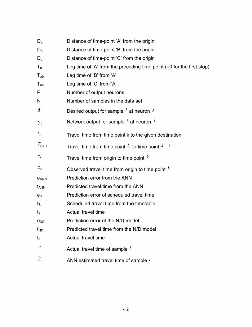
Da Distance of time-point ‘A’ from the origin
Db Distance of time-point ‘B’ from the origin
Dc Distance of time-point ‘C’ from the origin
Ta Leg time of ‘A’ from the preceding time point (=0 for the first stop)
Tab Leg time of ‘B’ from ‘A’
Tac Leg time of ‘C’ from ‘A’
P Number of output neurons
N Number of samples in the data set
ijd Desired output for sample at neuron i j
ijy Network output for sample i at neuron j
kt Travel time from time point k to the given destination
1, +kkT Travel time from time point to time point k 1+k
ks Travel time from origin to time point k
kz Observed travel time from origin to time point k
eANN Prediction error from the ANN
tANN Predicted travel time from the ANN
eS Prediction error of scheduled travel time
tS Scheduled travel time from the timetable
ta Actual travel time
eND Prediction error of the N/D model
tND Predicted travel time from the N/D model
ta Actual travel time
iy Actual travel time of sample i
iy ANN estimated travel time of sample i
viii

INTRODUCTION Overview This report summarizes the results of the work performed under the project title
“Use of Neural Network/Dynamic Algorithms to Predict Bus Travel Times under
Congested Conditions”. The objective of the project is to develop a
Neural/Dynamic (N/D) model to predict bus travel times at all major stops (time
points). The APC data collected from Bus Route 62 of NJ Transit was applied for
developing the proposed bus travel time prediction model. The travel times
between consecutive time points were predicted considering stochastic traffic
congestion, weather condition and ridership distribution. The predicted travel time
and actual bus travel time collected from APCs were then combined and fed into
the developed Kalman filtering algorithm, which enabled the predicted travel
times to be adjusted dynamically based on real time information (e.g., most
recent bus travel times, ridership, weather, and time of the day, etc.).
Background The Advanced Public Transportation Systems (APTS) program, one of the major
components in Intelligent Transportation Systems (ITS), was initiated by the
Federal Transit Administration (FTA) to encourage the applications of emerging
technologies in computers, communication, and navigation for promoting the
efficiency, effectiveness and safety of public transportation system. The APTS
technologies, such as Global Positioning Systems (GPS), Automatic Vehicle
Location Systems (AVLS) and Automatic Passenger Counter Systems (APCS),
have been implemented in various public transit systems to obtain real-time
information, including vehicle locations, speeds and occupancies. Such
information can enhance the capability of transit passenger information systems
assist proactive transit planning and management, and improve overall service
quality.
1
With the application of AVLS real-time information, such as vehicle locations and
speeds, can be estimated dynamically. However, only a reliable information
system embedded in a realistic prediction model can attract passengers to
access transit systems and use the predicted information (e.g., travel time) for
decisions of trip-making. Such information can be disseminated through Traveler
Information System (TIS) accessed by travelers at homes, work places, terminal
centers, wayside stops or on board through a variety of media (e.g.,
TRAVELLINK in Minneapolis, MN; PA.CIS in New York City, NY; AZTech in
Phoenix, Arizona, and SMARTBUS in Atlanta, GA).
NJ Transit faces increasing demand and the challenge to know ahead of time,
whether or not their buses are running on schedule. It is necessary to know when
buses will arrive at the designated onboard and destination stops. Bus travel
times are prone to a high degree of variability mainly due to traffic congestion,
ridership distribution, and weather condition. There is a need to develop a model
for predicting bus arrival times and improve the quality of information provided to
customers. Providing timely up-to-date transit information may reduce the
negative impact of schedule/headway irregularities on transit service. There is
also a need to examine the variability of bus travel times to prepare more
accurate schedules and assist transit agencies to restore service disturbances.
The bus travel time deviations between stops are usually caused by several
stochastic factors. Transit vehicle (e.g., buses) operations are frequently
disturbed by right of way competence with other vehicles, congestion on the
service route at different times of the day, intersection delays, variation in
demands, and dwell times at stops. The resulting impact of these factors on the
transit system comprises of bunching between pairs of operating vehicles,
increasing passenger waiting times (and hence risk of passenger safety),
deterioration of schedule/ headway adherence, uneven transition of inter-modal
transfers, increasing cost of operation and traffic delays. All these factors may
reduce the level of service and discourage riders to use the transit system. One
way to mitigate the impact is to provide accurate information of vehicle
2

arrival/departure times and expected delays at major stops. This will then enable
users either to present at the stop before the bus arrives or (if at all they are
already arrived at the stop) to effectively utilize their wait times (e.g., shopping,
making phone calls etc.).
The deployment of travel time prediction models in Advanced Traveler
Information Systems (ATIS) can benefit both transit providers and users. With
accurate vehicle arrival information, transit users may efficiently schedule their
departure time from work places/homes and/ or make successful transfers by
reducing waiting times at stops. Transit providers can manage and operate their
systems in a more flexible manner such as real-time dispatching and scheduling.
Therefore, proper control action (e.g., increase or decrease operating speed,
dwell longer times at some stops, etc.) can be determined, to maintain a
desirable level of service by dynamically restoring the disruptions in scheduled
headway.
The automatic passenger counter (APC) has been applied in NJ Transit buses.
The primary benefit of APC is the increase in both quantity and quality of
information collected. APC can link the time and location of a door open/close
event. This technology has provided a good platform to obtain reliable
information for predicting bus travel times between pairs of stops as well as
arrival times at stops.
Objective This research applied time and location dependent data automatically collected
by APC units installed in buses, including passenger counts and average travel
time between major bus stops. The objective of this study is to develop a
dynamic model (e.g., the integration of artificial neural networks and Kalman
filtering algorithm) that can predict bus arrival information with the use of real-
time and historical data. The following tasks have been conducted while
achieving the objective:
3

• Conduct extensive literature review in travel time prediction models.
• Identify geometric factors that affect bus travel times.
• Collect APC data to examine the bus travel times.
• Develop dynamic models that can adequately predict bus arrival times at
major bus stops, and
• Evaluate the accuracy of the developed predictive models.
Scope of Work and Organization In order to achieve the objective, extensive work has been performed and divided
into three phases: literature review, model development and model evaluation. In
Phase I, a comprehensive review of the current APTS applications was
conducted, while the potential prediction models that can be used for predicting
transit vehicle arrival/travel times were thoroughly investigated and discussed in
chapter 2. In Phase II, several tasks were conducted including preliminary
research of the studied patterns, collection of necessary data for developing
neural/dynamic (N/D) model. Chapter 3 discussed all the collected data including
APC data and GIS data provided by NJ Transit, weather data from National
Climatic Data Center (at Asheville in North Carolina and Boulder in Colorado)
and geometric data from the studied route. Chapter 4 was to identify the studied
patterns and select the appropriate prediction model software. Chapter 5
illustrated the procedure of data processing from data screening, calculation to
interpolation. Chapter 6 demonstrated the (N/D) prediction model development
and its refine procedures. In Phase III, the evaluation and analysis of the
developed prediction model was conducted. Chapter 7 provided statistical index
to evaluate the developed prediction models and analyzed the prediction results.
Chapter 8 concluded the research endeavor and proposed future research
direction.
4

LITERATURE REVIEW Introduction The application of automotive vehicle location (AVL) and automatic passenger
counter (APC) systems in transit is becoming more widespread in the United
States. The current practices, benefits, and technology associated with the real
time locations of buses, as well as, other associated technological components of
the advanced public transportation systems (APTS) are examined in this report.
Review of literature related to this issue has shown an increase in the usage of
the systems, particularly AVL and APC, in transit agencies across the United
States. This emergence has also led to an increase in the technology and the
quality of technology required for accurate information. Another major step
forward for the AVL systems is the increased and more accurate use of GPS
data to determine bus locations. The majority of the literature review listed
several perceived benefits as common reasons for installing this type of
technology on their buses. The most common benefits of AVL systems include
increased passenger safety, passenger satisfaction due to improved efficiency,
and improved efficiency for the transit-controlled systems. Difficulties or
problems experienced by those agencies that have implemented the system will
be examined. Similarly, a number of technological problems involving hardware,
software, and implementation are also discussed.
A number of studies and publications related to specific transit agencies are also
incorporated into this review, in order to determine the effectiveness of the
systems from a transportation standpoint. The primary focus will be on particular
agencies in order to determine how they are using and benefiting from the
implementation of different types of systems. Those agencies found to be using
AVL and/or APC systems range from small to large with varying degrees of use.
The cost of these systems also varies dependent upon the number of buses as
well as the different components utilized by each.
5
State of the Practice APTS Use and Options It was reported by the Federal Transit Administration (FTA) that in 1999 there
were 61 agencies utilizing AVL systems. (1) At this time there were also 93 more
agencies in the planning or implementation phase. The use of AVL is being
integrated with other systems to help improve the transit system for the
passengers. Some of these systems include: automatic vehicle
monitoring/control, emergency location, data collection, customer information,
fare collection, and traffic signal priority. Even though the technology is fairly
new it is already beginning to change. Earlier systems utilized the signpost
method for location; however, most systems today, nearly 70 percent, are GPS
(Global Positioning System) operated. The Federal Highway Administration
(FHWA) reported that GPS is the most widely used method and that the
accuracy has increased significantly (2) – it has improved from 100 meters to
between 10 to 20 meters in 2000. This increase is explained by the removal of
intentional degradation to the signal by the military. The improvement has led to
most agencies using GPS, however, for the sake of completeness the four types
that can be used are discussed below emphasizing the primary advantages and
disadvantages of each: (1)
• Signpost and Odometer (active and passive) – The vehicle reads a unique
signal from signposts in order to relay their position to dispatch. The
primary advantage is that the technology and use has been proven and
well established. The primary disadvantages are: (1) the need for
signpost, and (2) the system does not work if the bus is off route.
• Global Positioning System – Special receivers on the buses read
information from orbiting satellites. The main advantages revolve around
the accuracy and the fact that no wayside materials need to be purchased.
The only expressed disadvantage is that large buildings or tunnels can
6

block the signals. However, the use of the differential GPS would
somewhat correct this problem.
• Ground Based Radio – Receivers read information from a network of radio
towers in order to triangulate their position. Again the signals can be
obtained from anywhere without the need to purchase any wayside
equipment.
• Dead Reckoning –The use of the bus odometer and a compass are used
to determine the location. This system is often used in conjunction with
one of the other methods. Consequently, this system is rather
inexpensive, but is less precise.
Benefits A number of benefits, along with some problems are examined in order to
evaluate the effectiveness of AVL systems. The most common objectives of AVL
installation were to improve customer service, through improved safety, reliability,
and use of bus status information. A study conducted by the FTA (1) surveyed
numerous sites where ATPS was deployed and the usefulness of AVL systems
that are being used was evaluated. The sites surveyed were: Milwaukee County
Transit System (Milwaukee, Wisconsin); Ann Arbor Transportation Authority (Ann
Arbor, Michigan); New Jersey Transit (Essex County, New Jersey), King County
Department of Transportation, Metro Transit Division (Seattle, Washington); Tri-
County Metropolitan Transportation District (Portland, Oregon); the Regional
Transportation District (Denver, Colorado); and the Montgomery County
Transportation Authority (Rockville, Maryland). The transit agencies surveyed
stated the following as benefits of AVL and other system components:
• Improved schedule adherence and transfer coordination.
• Improved ability of dispatchers to control bus operations.
7

• Increased accuracy in schedule adherence monitoring and reporting.
• Assisted operations during snowstorms and detours caused by accidents
or roadway closings.
• Effectively tracked off-route buses.
• Reduced manual data entry.
• Monitored driver performance.
• Reduced voice radio traffic.
• Established priority of operator calls.
• Improved communications between supervisors, dispatchers, and
operators.
• Provided capability to inform passengers of predicted bus arrival times.
• Helped meet Americans with Disability Act requirements by using AVL
data to provide stop annunciation.
• Used playback function in investigating customer complaints.
• Used AVL data to substantiate agency’s liability position.
• Provided more complete and more accurate data for scheduling and
planning.
• Aided in effective bus stop placement.
• Used AVL-recorded events to solve fare evasion and security problems.
• Provided more accurate location information for faster response.
• Foiled several criminal acts on buses with quick response.
In order to apply the benefits to other agencies the following characteristics of the
survey sites should also be noted:
• AVL use ranged from 82 buses (Ann Arbor) to 1343 buses (King County).
• All utilized computer aided dispatching.
• All but King County used GPS or DGPS systems, King County used
signpost & odometer.
• All used mobile data terminals.
8

• APC were used or planned to be used on all but on Rockville, Maryland
and Denver, Colorado systems.
A number of particular agencies and programs also have detailed many benefits
from AVL and APTS use. The state of fleet control in the United States and other
countries was evaluated by the US DOT Operations Timesaver project (3) in
which a number of benefits were revealed from collected data. The following
were cited as examples of APTS benefits: fleet reduction (2-5 percent) due to
increased efficiency, improved travel time (Kansas City reduced scheduled travel
time by 10 percent), schedule adherence (Baltimore reported a 23 percent
improvement with AVL equipped buses), and improved safety due to less time
spent at bus stops. AVL also provided data for analysis that reduces the need
for staff to maintain schedules, estimating savings of $40,000 per travel time
survey to $1.5 million annually. Particularly, the schedule adherence
improvement was cited as: (4)
• Milwaukee County Transit System, Milwaukee, Wisconsin, reported an
increase of 4.4 percent, from 90 to 94 percent.
• Kansas City Area Transit Authority, Kansas City, Missouri, reported a 12.5
percent increase, from 80 to 90 percent.
• Regional Transportation District, Denver, Colorado, reported an increase
of between 12 and 21 percent on various routes. (4)
Aside from these, a number of smaller transit agencies also reported the effects
of AVL systems. A number of small and medium sized transit agencies were
surveyed for the Transportation Research Board to determine the benefits that
AVL systems and their components offered. (5) Most of the agencies surveyed
gained funding from “State and local Governments along with FTA.” The cost for
these smaller systems ranged from 50 to 750 thousand dollars. The number of
buses served ranged from 14 to 32. The analysis led to the conclusion that the
benefit of AVL systems is directly related to the annual ridership of the system.
9

In addition, most cost differentials are likely to occur with systems that have
“problems maintaining schedules and service reliability.” It is recommended that
AVL systems should be implemented to decrease passenger-waiting times to
attain the maximum benefit of the system.
Problems
The primary problems or difficulties experienced by most agencies dealt with
integration or implementation problems of the hardware and software. Another
problem, reported by the TCRP, from a survey of agencies found that funding
was the primary problem with procuring the system (6). Additional problems
include the need for more specialized staff to handle the updating, maintaining,
and controlling of the system. The process of implementing an AVL system
usually took more than a few years from design to full use. Most agencies had
not established a method to quantify the efficiency of their systems. Due to this
and the lack of comparable price comparisons it is hard to define the benefits of
the system quantitatively.
A number of issues needed to be addressed before APTS, particularly AVL, were
a beneficial investment. The primary issues revolve around integration of the
system, and are outlined below: (3)
• Institutional barriers – labor contracts, governmental rules, and political
directives can create barriers that prohibit cost effect introduction of such
systems.
• Infrastructure problems – Transit agencies are sometimes lacking
sophisticated technology, which makes integration of new systems
difficult. Installation of APTS is labor intensive, but is getting cheaper.
• Architecture/protocol – There is a technology compatibility problem and
integration with other transit technologies has been difficult.
10

• Integration issues – APTS devices alone are of limited value to
management decision-making, but when used in combination with broader
information systems they are very powerful.
Most of the issues mentioned are beginning to diminish. As more widespread
use of the systems evolve, the process of implementation is becoming easier.
Many of the agencies that have or are expecting AVL systems are purchasing
new buses with wiring for the system included.
Effects on the Workforce While the reported benefits of AVL systems are great, there is a certain degree of
training that is required for proper control of the system. Most research has
shown that after proper training, most workers find the systems beneficial. The
workers are able to complete their work more efficiently and accurately.
These human factors are very important and were the focus of a United States
Department of Transportation Report in 1999. (7) The effects of real time vehicle
location systems on the employees of the transit agency were examined. The
study was based on the new Computer Aided Dispatch/Automatic Vehicle
Locator (CAD/AVL) system at Denver’s Regional Transportation District (RTD).
The data collected in 1996 and 1997 were compared with that collected before
installation of the system. The collected data include frequency of
communications, number of personnel per unit of service, procedures and
communication, the attitudes of the dispatchers, street supervisors and bus
operators. The employees had to learn how to use and integrate the new
technology into their jobs. The analysis found that this new knowledge provided
additional information to the personnel, but did not change their responsibilities.
The report also found that dispatchers had to make fewer requests for
information and could make their decisions more accurately and easily.
Operators had more “accountability” in controlling the buses and their schedules,
11

but the dispatchers’ workload increased due to an increased number of received
calls. It was also stated that street supervisors have more duties than before;
however, their need to observe traffic conditions in the field became non-existent.
Overall, almost everyone found that the newly provided real-time information led
him or her to more accurate information and decisions.
A study that looked at the same transit system in Denver, Colorado offers
information about the impacts of an AVL system on the transit employees. (8)
The report analyzes the effectiveness of an AVL system installed in Denver,
Colorado by the RTD. The system was installed in 1993; however, it was not
used until 1996 due to a number of difficulties. After most of the installation was
complete and the system was being used, a number of employees were
surveyed to determine their feelings about the system. Operators, dispatchers,
and field supervisors were all surveyed. Most of those surveyed found the
system to be easy to use, helpful in emergencies, and accurate and reliable.
Applications In order to thoroughly examine the effect APTS systems, specific examples need
to be examined. The following sections detail the use of specific systems,
programs, or technology to explore the scope and benefit of AVL and/or APC
technologies.
Nextbus The Nextbus System provides services to a number of different agencies.
Nextbus Information Systems provides arrival information that is updated at
regular intervals. (9) GPS satellites are used to relay the location and other
information to the AVL on the buses. Using typical traffic patterns and normal
bus stops, Nextbus is able to predict arrival times for the buses at each stop.
These arrival times are updated regularly to ensure comfort and security of the
riders. Predictions are made available to the web, signs at bus stops, Internet
12

capable cell phones, and Palm Pilots. Nextbus projects include MUNI-Metro
Light Rail Vehicles, AC Transit-Alameda County Transit in California, Fairfax,
Virginia, METRO Transit-Oklahoma City, Vail Transit, Massachusetts Bay
Transportation Authority, MTD-Santa Barbara, and many others. The following
descriptions are from the websites of the individual agencies and include relevant
information concerning the use of Nextbus systems:
Arlington (10) On September 11, 2001 an 18-month, $100,000 pilot
program in Arlington County, Virginia will install the Nextbus technology in
the eight buses that run the 38B line. Real time information messages will
be relayed on 9 new electronic signboards.
AC Transit (11) The AC Transit in Almeda County in California is using the
Nextbus technology as pilot project. The system is being used on the
heavily traveled San Pablo corridor (72, 72L, and 73 lines). Their project
enables riders to get bus information over the Internet.
Fairfax CUE (12) The City-University-Energysaver (CUE) Bus System that
serves the city of Fairfax and George Mason University in Virginia is
equipped with Nextbus equipment that uses computer modeling to predict
bus arrival times. Each vehicle is equipped with a satellite-tracking device
that allows bus arrivals to be estimated within a minute, with 95 percent
accuracy. CUE bus system provides information that can be relayed to
the web, signs at bus stops, Internet capable cell phones, and Palm Pilots,
to provide real time information to patrons.
Vail Bus Service (13) Beginning on June 23, 2001 the Town of Vail,
Colorado started using the Nextbus System. The following areas are
using the systems: Vail Village, LionsHead and Golden Peak corridor.
Location information is transmitted every 90 seconds to the AVL system at
13
the central dispatch center. The town is currently evaluating options that
would add the Nextbus system to outlying areas of Vail.
San Francisco Municipal Railway (MUNI) (14) A 9.6 million-dollar
contract was awarded to Nextbus to install their technology on all of their
transportation equipment. The equipment was tested on light rail lines
and also on one bus line, 22 Filmore, that serves 20,000 passengers a
day. The system will provide GPS equipment on all buses and trains.
Cable cars and streetcars in San Francisco would also use the
technology. Part of the project also includes installing 430 electronic
informational signs. GPS “information is sent to a centralized server and
compared with historical information and the bus or train arrival is then
projected and available via wireless devices such as phones and
handhelds.” The project is expected to take nearly five years to fully
complete on all lines.
Tri-Met – Portland, OR The Tri-Met Transit Tracker system provides real time transit vehicle arrival time
information to patrons on stations of selected routes. (15) The total cost of the
project (Transit Tracker) is estimated to be $ 4.5 million with the City of Portland
paying $ 3 million and Tri-Met paying $1.5 million. The Transit Tracker system
will work with a dispatching system that is already in place, which utilizes AVL
and APC technologies. The initial system has led to many improvements:
• Overall improvement of on-time 69 percent to 83 percent.
• Early arrivals declined from 15 percent to 5 percent.
• Schedules have improved using information provided by the Bus
Dispatching System.
14
The Transit Tracker system was expected to be used to relay real time
information at 50 rail stations and 250 bus shops initially. This will be followed by
deployments of approximately 50 stations per year. The system will also provide
the information to the Internet. The following improvements will also be
implemented in the near future for use with the existing AVL and APC: Transit
Signal Priority, LIFT Scheduling System Upgrade/Electronic Data Transmission,
Automated Stop Announcements, Bus Dispatch System Upgrade, Scheduling
System Software Procurement, Radio and Microwave Replacement Project (with
Motorola Gold), DISPATCH Operations Utilities Program, LIFT Program
Integrated Voice Response, and Automated Yard Mapping and Vehicle
Assignment.
AOS – Ann Arbor, MI In Ann Arbor Michigan a fully automated Advanced Operating System (AOS)
began to use in 1998. (16) It was expected to offer a “fully integrated public transit
communication, operation, and maintenance system.” The Ann Arbor Transit
Authority (AATA) serves over 4 million riders a year, with 27 bus routes that are
offered 7 days a week, 24 hours a day. Each bus utilizes the following
equipment:
Advanced Communications: Each bus has an 800 MHZ radio and onboard
computer that minimizes “voice transmissions by providing data messages that
summarize vehicle status, operating condition, and location.” The driver can also
switch to a voice system. The system is responsible for relaying all information
and for onboard announcements.
AVL: Each bus uses GPS to determine their own location, accuracy is within one
to two meters. An insertable memory card stores the bus routes and compares
them to the accurate time given by the GPS system. If this comparison
determines the bus will not be on time the onboard computer notifies the
Operation Center and the AVL relays the announcement to the internal next-stop
15

signs and announcement. The AVL also integrates location data with fare
collection, passenger counters, and engine data that are controlled electronically.
Dispatchers are able to manage the system and assist drivers by inserting
overload vehicles in the system or offering route suggestions.
Emergency System: An onboard emergency system allows drivers to alert
dispatchers of an emergency, who in turn can note the bus positions and notify
the proper authorities.
En Route Information: Onboard the bus stop announcements, date, time and
route are relayed to patrons. The driver can also activate timed and periodic
announcements.
Geographic Information System: The Rockwell MapMaster is also a part of the
AOS on AATA buses. It allows you to enter locations of bus stops and routes.
The data can be “imported to the route generator GIS system.” The GIS system
then creates schedules time points, announcement points, transfer points and
bus stops by route.
Computer-Assisted Transfer Management: This system, TransitMaster, allows
drivers to request transfers that are then calculated by the dispatch computer that
advises the drivers whether a transfer is possible or not.
Other benefits provided by AOS include fare collection, ability to relay real time
information to patrons, APCs, video surveillance (3 cameras on each bus), and
vehicle component monitoring. The video surveillance has lead to improved
cleanliness on AATA buses. Rider information is provided through the use of
public access cable, monitors at the transit center, and the web. Reviews of the
system have found improved departure time accuracy, potential long term cost
savings, and an online survey of users found the system very favorable. The
study also found that its AVL system has a median positional error of 85 meters,
16

ranging as high as 580 meters and as little as 3.25 meters. The inaccuracy was
believed to arise from “differential GPS correction deterioration in outlying areas”.
MyBus – Seattle, WA The Transit Watch system is an ITS Research Program at the University of
Washington (17) for the King County Metro Transit. It is part of the Federal
Highway Department Smart Trek: Intelligent Transportation Infrastructures,
Model Deployment Initiative. Computers have been installed at the Northgate
and Bellevue Transit Centers where Transit Watch has been available to bus
riders since July 1998. The Transit Watch program includes 4 primary parts: (1)
the prediction server (Predictor), (2) data distribution server, (3) the client display
applet (Transit Watch), and (4) a database. The entire system utilizes an object-
oriented Java Language. The Predictor predicts the arrival times. A Predictor is
available at each location that the Transit Watch provides an arrival prediction.
The Predictor receives data from an AVL and reads the active trips, trips that are
scheduled to depart the prediction site in a particular time window. A trip tracker
“uses a tracking algorithm to combine the current position of the bus with
historical data about the trip to predict the arrival time.” When new data is
received, the predicted time is updated. Information is collected and can be
displayed on the Internet or web-capable phones, which is the function of the
second component. The third and fourth components backup and save
information for subsequent uses.
Dailey and Maclean (18) described the ability of the MyBus system to forecast
arrival and departure times, focusing on the system and how it works to predict
the necessary information. The algorithm used by the predictor will be discussed
in a later section.
RTD – Denver, CO RTD is an agency that was previously mentioned in this report in regard to the
workforce. The Department of Transportation (8) further analyzes the
17

effectiveness of an AVL system installed in Denver, Colorado by the Regional
Transportation District (RTD). The system was installed in 1993; however, it was
not used until 1996 due to a number of difficulties. After most of the installation
was complete and the system was being used a number of employees were
surveyed to determine their feelings about the system. Operators, dispatchers,
and field supervisors were all surveyed. Most of those surveyed found the
system to be easy to use, helpful in emergencies, and accurate and reliable.
Several did mention that the system was not working properly at all times. This
was explained by the difficulties of installation. A survey of patrons was also
conducted, finding that 90 percent of passengers thought the bus service was
good or better.
Along with the surveys, a cost analysis was also conducted. The final cost of the
completed system was 10.4 million dollars, with in-vehicle hardware accounting
for half of that cost. The overall results of the system were found to be
successful; however, there were a number of problems. The system has helped
workers, patrons and improved accuracy, but the RTD did not use the improved
data to improve schedules. This fact was used to explain a minimal increase in
efficiency. The system was not used to its fullest ability due to the functional
problems experienced in the beginning of installation.
Other Practices The FTA (1) documents the use and deployment of all types of intelligent
transportation systems, including that used for transit agencies. The report
states that the benefits of using an AVL system are improved dispatching and
operational efficiency, improved reliability of service, quicker response to
disruptions in service, quicker response to criminal disruption, and extensive
information at a lower cost that can be used for future planning. In addition a
number of cities and agencies were used to evaluate the use of AVL systems.
The cities are listed below:
18

Essex County, New Jersey – The New Jersey Transit (NJT) AVL system has
been in place and working since early 1998. NJT purchased a signpost and
odometer system as well as a statewide 23-tower radio system from Motorola.
Two thousand buses on 26 lines in Essex County are operated fully with the AVL
system. It was also reported that there were only about 100 of the original 600
signpost remaining due to weather problems. Due to this fact AVL is not
available Statewide, but radio communication is.
Chicago, Illinois – An AVL system utilizing dead reckoning with DGPS correction
is used by the Chicago Transit Authority (CTA) on 1210 of the agencies 1872
buses. At the time of the report emergency location and text messaging were
available, while new radios were needed for further capability. It was reported
that the CTA has 12,900 stops and coding of the first 1,000 took 3 months. Once
this is completed 254 buses will operate with both the AVL and new radio
systems. CTA expects to provide the equipment on the rest of the fleet as new
buses are acquired. At the time of the report they had a contract with NOVA for
150 buses furnished with wiring compatible for the installation of AVL equipment.
Baltimore, Maryland – A phased implementation plan is being utilized by the
Maryland Mass Transit Administration (MTA) for acquiring their AVL system.
Fifty buses were initially tested using the Loran-C AVL system. Additionally MTA
has purchased a DGPS system at an estimated cost of $15,000 per bus. This
includes a new radio system consisting of the radio and base station equipment.
The project included AVL equipment for 380 of the 868 vehicles, while the rest of
the fleet will be equipped as new vehicles are purchased – sixty-five new buses
equipped with AVL were expected in late 1999 at a cost of 8 million dollars. The
plan includes passenger information being available by phone, along with limited
information available by sign. MTA expects to save 2-3 million dollars annually
by the fourth to sixth year of operation via purchasing, operating, and maintaining
fewer vehicles.
19
Rochester, Pennsylvania – The Beaver County Transit Authority (BCTA) are
upgrading their Loran- C system to a DGPS system. They hope to upgrade the
system that has been in existence since 1991 to the DGPS system by 2000. All
20 of BCTA’s buses will be equipped with the AVL system, and all new buses will
be equipped with the appropriate wiring to install the system. Along with the
usual benefits of timesaving, the BCTA hopes to monitor contractors that operate
the system and use it to investigate customer complaints.
Of other interest, the report also offers discussion of the Operations Software for
Fixed-Route Bus Operations, focusing on the most commonly used system-
Computer-Aided Dispatch (CAD). The CAD system is used for bus service, as
well as operations planning. Customers are able to use it for itinerary planning
and transfer connections. The report discusses implementation challenges and
noted that most of the agencies surveyed were still learning how to use the
system effectively. Most problems dealt with compatibility issues involving
missing information and oversensitive location algorithms.
Automated Passenger Counters (APC) system is also discussed in detail in this
report. The primary benefits of the APC’s are the reduced cost to collect
information and an increase in the amount and quality of the information
collected. APC make it possible to reduce or eliminate the need for manual
checkers. Several cities using APC’s are examined in the report and some are
discussed here briefly:
Columbus, Ohio – The Central Ohio Transit Authority (COTA) began using APCs
in 1984, when it acquired 37 units. The units purchased from Urban
Transportation Associates for $171,000, was enough to equip about 10 percent
of their fleet. COTA reported a 95 percent accuracy of the counts, and found the
system very useful. COTA planned to upgrade their system with APCs that use
vertically pointed infrared beams mounted in the roof of the vehicle to count
20

passengers. The data will be transmitted in real time, and combined with AVL
data to be used for planning and to improve schedules.
Atlanta, Georgia – The Metropolitan Atlanta Rapid Transit Authority (MARTA)
has installed 74 APCs on AVL-equipped buses. MARTA reported that their data
is between 80-85 percent accurate. They use the counters to generate a great
deal of information but feel that the systems should not replace manual checkers.
As a result, they have not reduced the number of manual checkers that they
used previously. They also reported that APCs are the most difficult piece of
APTS technology to upkeep, and that only about 40 of the 74 counters provide
good information on any given day. Despite such maintenance problems they
estimated a savings of 1.5 million dollars in operating expense per year.
Baltimore, Maryland – The Maryland Mass Transit Administration (MTA) has
used APCs on 25 buses since 1997. The units count passengers using
horizontal infrared beams and were acquired from Urban Transportation
Associates. The MTA plans to purchase 75 more APCs in order to equip over
10 percent of their fleet.
Newark, New Jersey – New Jersey Transit plans to purchase 170 APC units for
its buses. The units will be considered as part of their AVL system. Data
transmission is planned to utilize wireless download after the bus returns to the
garage. The report states that the APCs will help NJT generate a greater volume
of information and more accurate data to help them better understand ridership
and to improve market research.
Developed Applications Benefits and uses of the AVL system are also reviewed in relation to some of the
cities where its use is being proposed. (19) These cities include Albany, NY,
Eugene, OR, Los Angeles, CA, and Pittsburgh, PA. Each of the city’s projects
21

incorporates the use of AVL and serves thousands of people a day on their
transit system. The projects are all in the design or implementation phase. In
Albany (20), the Capital District Transit Authority's primary bus route, with 20
percent of the system's passengers, runs 16 miles from Albany to Schenectady.
The project for Albany includes signal coordination to optimize bus signal priority.
They hope the program will lead to shorter bus route times, improved service to
three major routes and higher frequency service. In Los Angeles, Metro Rapid
began on June 24, 2000 with the start of service of two routes, Whittier-Wilshire
Boulevard (line 720) and Ventura Boulevard (line 750). The Metro Rapid is
expected to expand into as many as 15 to 20 new express lines. The Metro
Rapid is using ITS including AVL to increase the efficiency of the transit system.
Similarly, many of the other cities are beginning with smaller testing areas, with
plans of widespread expansion.
Other Technologies During the course of implementation for the AVL and APC systems a number of
other technologies have emerged, some of which were previously mentioned.
Another product gaining attention is the Transit Integrated Monitoring System
(TIMS). (21) This technology revolves around the use of Passenger Tags. The
tags are actually radio frequency identification cards, which “act as bus passes.”
The cards are devised to integrate AVL and APC technologies. The tags are
used to uniquely identify passengers, and then keep track of their position using
GPS satellites that monitor the bus. The card is swiped as the passenger boards
the bus and again activated as the passenger leaves the bus. From this the
arrival and departure times to be recorded, leading to improved information
regarding “origin destination pairs, passenger transit times, and schedule
adherence.” Along with this valuable information, the cards can be used as a
fare card, acting as a debit card or other billing techniques. The three primary
goals of the project as outlined by the author are:
22
• Advanced systems for transit vehicle location, identification, and
management.
• Improved methods of data collection about or from transit users.
• Advanced systems for fare collection and control systems.
Costs and Communication The John A. Volpe National Transportation Systems Center studied several
agencies that utilize AVL systems. (4) The study focused on a number of variables
including cost. They found the median cost per system was reported to be
$8,000, with a range from $1,200 to $23,000. The wide range of cost was
explained by varying functions performed by each system. The study found that
only operations software and pre-trip automated passenger information had
widespread use. It is believed, however, that many other related technologies
will reach widespread or moderate levels of use in the near future. This is based
on the number of agencies that have plans to implement the technology.
A TCRP synthesis also comments on the cost of implementing advanced
technology systems. (6) Based on this information gathered it was concluded that
the technology is increasing as agencies begin using GPS type information,
rather than the older signpost method. As a result, the performance of the
infrastructure and onboard equipment has increased. Consequently, GPS
systems, which allow for complete coverage, are now being used in most new
installations. A major cost of the system, one to two-thirds, involves integration
of a communication system. One particular agency, MTD, which provides real-
time information to the public, reported a two percent increase in ridership with
increased customer satisfaction. At the time of the report many agencies did not
provide real time information to their passengers. Also at the time of this report
an average cost of $13,700 per bus was reported, with some smaller agencies
paying more due to fewer units purchased.
23
As mentioned previously, the influx of information is insignificant without
increased communication abilities. Communication of real time information
through wireless phones, electronic message boards, websites, and personal
digital assistants are becoming popular. The Metro King County MyBus site, for
example, has had a significant increase in the number of hits since providing real
time information. Other sites offer real time maps and bus information to keep
their patrons informed.
Prediction Algorithms Many forecasting methodologies have been applied to transportation research,
such as prediction of traffic volume, travel time, etc. Particularly, various bus
arrival time prediction models have been developed using different
methodologies, such as time series, artificial neural network, and Kalman filtering
algorithm.
MyBus Application
The predictor for MyBus utilizes three pieces of information including that
collected from the posted schedule, a set of previous trips, and the AVL stream.
The AVL system supplies information every one to three minutes per vehicle,
while the previous trips provide statistics to the systems algorithm used for
prediction. The prediction algorithm uses the Kalman filtering technology.
Specifically, vehicle location, time, and time until arrival were considered as state
variables. The reported position and its time measurement were observables.
The predictor in Seattle is capable of making 25,000 predictions every 10
seconds. (18) The time and distance to the destination, the bus stop, are
calculated for each prediction. The deviations were modeled as a probability
surface to show the accuracy of the system. (22) The analysis made by the
authors found the system to reduce errors by 50 percent to 75 percent, as
compared to the schedule alone.
24

Since the observations of vehicle location can only be recorded at irregular
intervals. Typically, linear interpolation was applied to obtain estimated arrival
times. Using the latest bus location and time data, the Kalman filter continuously
predicts the arrival time.
Blacksburg Transit Application Algorithms were developed for a transit traveler information system in
Blacksburg, Virginia to predict bus arrival time at rural setting (23) GPS data was
gathered at variable time intervals, including location and time label. However,
because of its inherent constraints (no fixed sample period, erroneous reports),
the accuracy of the prediction is compromised.
Four algorithms were developed in the study based on various data sources as
input:
• GPS bus location data only
Arrival time at the downstream time point is estimated based on the arrival
time at the upstream time point and historical travel time between them.
• GPS bus location data and bus schedule table
Bus arrival times at nearby downstream time points are based on GPS
data while assuming current delay has little impact on the arrival time at
downstream stops that are far away.
• GPS bus location data, bus schedule table, and delay
This algorithm takes into account the fact that bus drivers tend to adjust
their speeds (within speed limits) in order to arrive on time. So the current
delay of the bus is taken as an input.
• GPS bus location data, bus schedule table, delay, and time check point
This algorithm is based on the 3rd algorithm with an added input as dwell
time at time check point since it is usually much longer than that at other
stops.
25
Performance of these algorithms was compared based on criteria including
overall precision, robustness, and stability. The 4th Algorithm outperformed all
other ones. However, it was also concluded that the algorithm performance was
also location dependent.
Texas A&M University TransLink Lab Two algorithms, time-based and distance-based, for predicting travel time of
campus buses were developed at the TransLink Lab of the Texas Transportation
Institute at the Texas A&M University. (24)
In the time-based model, bus route between two stops was divided into a series
of one minute zones, and estimated arrival time can be obtained by locating the
bus on the route to see how many one-minute zones it needs to traverse to reach
the stop. This method is based on historical travel time data and therefore
cannot capture real time traffic variations.
The distance-based algorithm uses the distance to a bus stop and time of the
day as independent variables. Particularly, the algorithm takes into account the
variations in running speeds and dwell times of a bus both during class and
during the pedestrian congestion of class breaks.
Comparisons of the prediction results with actual arrival time showed that the
distance-based algorithm had a better performance, i.e., with relatively small
deviation. However, it was more complex and cost more to calibrate.
NJ Transit Bus Route 39 Chien et al. (25) developed a bus arrival time prediction model that combined the
forecasting capabilities of artificial neural network (ANN) and dynamic filtering
techniques. ANN was chosen because it was proved to be a powerful tool to
simulate complicated systems, especially those with large number of variables
26

and complex correlations among these variables that are difficult to be explicitly
modeled. Dynamic filtering technique was applied to adjust the ANN prediction
output using most recent readings from the bus location as well as traffic
information.
This model was established based upon simulation data generated from a model
that was calibrated and validated on New Jersey Transit Bus Route 39. The
simulation model was able to provide various traffic data such as volume,
passenger demand, speed, delay, etc. as the input to the prediction model.
Various combinations of these variables were experimented in the ANN training
process, and the most relevant ones were identified.
Two algorithms, link-based and stop-based, were developed. The former
assumes additive link travel time/cost, and generally defines the segment of the
route that is between two adjacent intersections as a link. The latter is
established based on aggregated data at each bus stop including demand and
volume, speed between to adjacent stops.
Performance evaluation showed that link-based algorithm outperformed the stop-
based one when the number of intersections between a pair of stops is relatively
small, while the latter one accommodated the stochastic conditions at further
downstream stops better.
Media for Information Dissemination This section will discuss the media for information dissemination from Federal
Transit Administration (FTA). (26) The types of media that are of interest in the
literature include those listed below in Table 1. These media have been
designated either interactive or non-interactive.
27

Table 1Media for Information Dissemination
Interactive Media Non-Interactive Media
Internet DMS’s
Interactive voice response (IVR) via telephone Video monitors
Interactive kiosks Fax
PDAs Non-interactive kiosk
Wireless Application Protocol (WAP)-enabled Telephones (voice information)
Mobile Phones Cable television
Different from Non-interactive media, interactive devices (such as kiosks and the
Internet) allow users to timely get the information they are seeking. Within the
two types of media, DMS and the Internet, respectively, were referred with the
most in the literature. Hence, more extensive evaluations of the other types of
media may be required in the future to arrive at a better understanding of these
systems.
Peng and Jan (27) evaluated dissemination media for real-time transit information
(e.g., pagers, the Internet, and PDAs). For each media type, they provided a
general description, including its advantages and limitations. all the studied
media were evaluated based on their accessibility, versatility and interactivity,
information-carrying capacity, user friendliness, cost to install, cost to use, and
ease of implementation. The Internet and kiosks were found to be the best
media overall. DMS and closed-circuit television (CCTV) were considered good
dissemination media because of their modest cost and flexibility in the variety of
provided information. PDAs and automated voice annunciators were promising
technologies for real-time transit information systems, but were not ready for
implementation when the paper was published. Reviews on interactive media are
discussed below:
28
Internet As part of the Smart Trek Metropolitan Model Deployment Initiative (MMDI) in the
Seattle, Washington area, two new applications were created to provide real-time
transit information. (28) Two types of media were used to relay the information to
the transit passengers: (1) on the Internet and (2) at the transit center. Busview
displays the real-time location of all the transit vehicles operated by King County
Metro. Transit Watch is a real-time arrival prediction system suitable for
deployment in transit centers. Busview and Transit Watch are designed to
operate over the Internet.
The Transit Watch project deployed an Advanced Public Transportation System
APTS /ATIS that predicts the arrival status of transit vehicles. This prediction
results in one of four states: (1) On Time, (2) Delayed “n” Minutes, (3) Departed,
and (4) No Information. The goal of the project was to develop an interface that
promotes the use of transit by reducing the stress inherent in transfers. This
project leverages the ITS Backbone component of the SmartTrek MMDI project.
This project was originally designed to be deployed at three transit centers, but it
has since been made available on the Internet as well.
Stuart Maclean and Daniel Dailey (29,30) discussed the dissemination of real-time
transit information to a WAP cellular phone. The use of WAP phones was an
extension of the ongoing Internet-based MyBus program in Seattle, Washington.
In that study, challenges such as limited display area and capability of using
WAP phones for real-time information were discussed. To compensate for the
phone’s physical restrictions, MyBus maximized its use of the screen by
combining information, such as scheduled arrival time and departure status, into
one data field. Future work for this project includes formatting bus arrival data for
PDAs.
29

Dynamic Message Signs (DMS) DMSs at bus stops are used mainly to provide arrival or departure information to
reassure the customer that s/he is waiting for the right vehicle in the right place
and to inform him/her the vehicle arrive times. In many cases, bus stop displays
also are used to provide static information about the transit service and to display
advertisements. The sample systems using DMSS include VIA system
(Visualizzazione Informazioni Arrivi) in Turin, Italy, COUNTDOWN system in
London, and Los Angeles Metropolitan Transportation Authority (MTA).
Interactive Voice Response (IVR) IVR telephone information systems allow customers to call a single phone
number and navigate a menu for needed information. Previously, transit
customer service operations relied on agents to provide various types of
information over the telephone. For many years, automated telephone
information systems assisted agents in answering routine questions. The new
systems eliminate the need for agent involvement in many information
requests.(31) One problem with IVR systems is that they do not always have good
voice recognition. However, speech recognition technology has improved
recently. Another difficulty noted in the literature is that some systems
incorporate automated distribution features for information that would be too
time-consuming to provide over the telephone. In these cases, information can
be sent via fax or e-mail. (31) One of the real-world systems applying IVR is the
Bay Area’s TravInfo® project.
Interactive Kiosks Kiosks can be located in a variety of places, including near public transit, in
stations, at stops, or in other high foot-traffic locations (e.g., in shopping malls).
They can also be located at places with high concentrations of people, such as
public buildings and tourist locations. The literature suggests that information
available via kiosks usually includes: Travel information, (e.g., optimum route,
30

itineraries, and arrival times at specific locations) and general information (e.g.,
scheduled activities in the city or metropolitan area).
Several functional characteristics of kiosks should be taken into account when a
kiosk is being considered. These characteristics include:
• Simplicity of the user interface.
• Provision of useful and understandable answers to the user request.
• Effective location.
• Appropriate housing.
• Efficient maintenance.
• Use of standards.
According to the literature, kiosk users mainly have problems with the touch keys
and/or the touch screen, as well as with the time required to wait until they get
the system response. However, the general level of satisfaction is rather good.
Video Monitors
According to Advanced Public Transportation Systems: The State of the Art
Update 2000, (31) video monitors are often used when a large amount of
information needs to be displayed and where flexibility in using graphics, fonts,
and color is needed. A video monitor providing real-time arrival updates would
be less suited to a central display near a group of bus berths, since transit users
might be uncomfortable moving away from the berth and losing their places in
line to get close enough to read the display.
Personal Digital Assistants (PDA)
Hand-held PDAs recently appeared as information media in the transit field. The
traveler can consult them at any moment anywhere. PDAs can be used to obtain
pre-trip and en route information. Advanced Public Transportation Systems: The
31

State of the Art Update 2000 (31) claimed that one issue with PDAs is the
reluctance of customers to pay for traveler information via pagers or handheld
computers. However, private sector companies are devising ways to provide
more “value added information,” such as personalizing information on a traveler’s
commute by informing him/her when transit delays are occurring.
32

DATA COLLECTION
APC Data The collected APC data of Year 2002 consisted of January Pick (from January to
June, 2002), June Pick (from June to September, 2002), and September Pick
(from September to December, 2002), which were retrieved from the APC
database at NJ Transit. The OD pair on Route 62 between Woodbridge Center
Mall and Newark Penn Station was selected as the studied route, in which bus
service was provided by different patterns. Bus running on different patterns will
be assigned a unique pattern abbreviation. For example, there are a total of 10
patterns recorded on both in and out-bound trips for this specific OD in each pick
data. All attributes in each APC record that might be related to this project are
summarized in Table 2:
GIS Data With the collected APC data, GIS could efficiently capture, store, retrieve, update
and display all these information. In addition, GIS could perform advanced
analysis on segment and route level using APC data and enhance demonstration
function. Such applications can improve the quality of bus operational data and
strengthen the database validation for travel time prediction and planning. Thus,
it has proved to be an efficient and a powerful tool for analysis data in public
transit.
33

Table 2 APC Data
Variable Description
Sched Run Time Scheduled run time of the bus in the entire trip Actual Run Time Actual run time of the bus trip Sched Start Scheduled start time of the trip Sched End Scheduled end time of the trip Actual Start Actual start time of the trip Actual End Scheduled end time of the trip Time Of Day Starting time of the trip Transit Day Date of the service Open Time Recorded bus door opening time Close Time Recorded bus door closing time Stop Description Stop description Stop Sequence A unique number attached to all intended stops along the
route. It has a value of 10 at the origin and increases in increments of 10 for subsequent stops.
Time Point ID Time Point indicator number Direction Service direction (Inbound or Outbound) Trip Status Trip status (Start or End) Lat Latitude Lon Longitude On Number of boarding passengers at a stop Off Number of alighting passengers at a stop Stop Distance Travel distance between two consecutive stops Dwell Time The bus door open time at any particular time-point. They
are derived from the original data as, the cumulative time that the vehicle halted at all intermediate stops.
Leave Psgr Load Number of onboard passengers when the bus leaves a stopArrive Psgr Load Number of onboard passengers when the bus arrives a stopLeg Time Inter-stop travel time. The difference of door open time at a
subject stop and door close time at previous stop. Origin Origin of the trip Destination Destination of the trip Pattern ID 4-digit number associated with each pattern in each pick
data file.
Trip Index Unique index associated with a trip
34
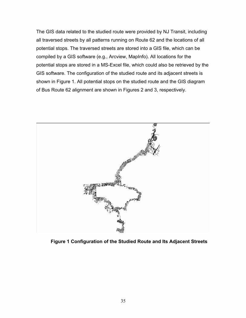
The GIS data related to the studied route were provided by NJ Transit, including
all traversed streets by all patterns running on Route 62 and the locations of all
potential stops. The traversed streets are stored into a GIS file, which can be
compiled by a GIS software (e.g., Arcview, MapInfo). All locations for the
potential stops are stored in a MS-Excel file, which could also be retrieved by the
GIS software. The configuration of the studied route and its adjacent streets is
shown in Figure 1. All potential stops on the studied route and the GIS diagram
of Bus Route 62 alignment are shown in Figures 2 and 3, respectively.
Figure 1 Configuration of the Studied Route and Its Adjacent Streets
35

N
Figure 2 Potential Stops on the Studied Route
Figure 3 Alignment of Bus Route 62 in GIS
36

Weather Data The weather information was obtained from the National Climatic Data Center (at
Asheville in North Carolina and Boulder in Colorado). Newark International
Airport Station in NJ is selected as the observation station because it is the only
station that collected weather data covering the studied route. The weather
information includes hourly temperature (e.g., dry bulb temperature), precipitation
(e.g., rainfall and snowfall), and sky conditions (e.g., visibility and wind speed)
To access the hourly weather information, a step-by-step procedure is listed
below:
Step 1: Log in National Climatic Data Center (NCDC) website at:
http://lwf.ncdc.noaa.gov/oa/climate/stationlocator.html. The webpage of the site is
shown in Figure 4.
Figure 4 NCDC Weather Observation Stations
37

Step 2. Input station name “Newark Airport Station” and hit "Search". A new page
is shown in Figure 5.
Figure 5 Newark International Airport Station
Step 3. Click "DATA" in the upper right portion of the page in figure 5. A new
page is shown in Figure 6
Step 4. Cli
page is sho
Figure 6 Weather Information of the Selected Station
ck "Hourly/Daily Data, Local Climatological Data (Unedited)". A new
wn in Figure 7.
38

Figure 7 Time Period Selection for Querying Weather Information Step 5. The hourly weather information for the selected month can be obtained. A new page is shown in Figure 8.
Figure 8 Example of Collected Weather Information After applying this procedures, the historic weather information at selected
locations could be retrieved from the website. The attributes of the data available
from NCDC are listed in Table 3, in which the precipitation data variable is used
to develop prediction model in this study.
39

Table 3 Weather Data Provided by NCDC
Date Time Station Type Maintenance indicator Sky Condition
Precip.Total Visibility Weather Type Dry Bulb Temp (F)
Dew Point Temp (F)
Wet Bulb Temp(F)
% Relative Humidity Wind Speed(KT) Wind Dir Wind
Char.Gusts(KT)
Val. For Wind Char. Station Pressure Pressure
Tendency Sea Level Pressure Report Type
Field Data Since the geometric characteristics of the studied route may affect bus travel
times, it is necessary to collect related information along the route. While visiting
the studied site, the research team rode the bus to record the number of left/right
turns, the numbers of intersections with and without signals, and the bus
exclusive lane on each segment between consecutive time points, which might
affect the bus travel time. There were no bus exclusive bus lanes on the studied
route, and all collected geometric information is shown in Tables 4, 5 and 6.
Table 4 Time Points Description on the Timetable
Number Time Point Description
1 PENN STATION BUS LANES
2 BROAD ST & BRANFORD PL
3 NWK AIRPORT TERM A
4 FEDERAL EXPRESS - NEWARK AIRPORT
5 IKEA
6 BROAD ST & W JERSEY ST
7 SAINT GEORGES AVE & WOOD AVE
8 IRVING ST & BROAD ST
9 W INMAN AVE & ST GEORGES AVE
10 INMAN AVE & WOOD AVE
11 NJT METROPARK STATION
12 WOODBRIDGE CENTER MALL
40
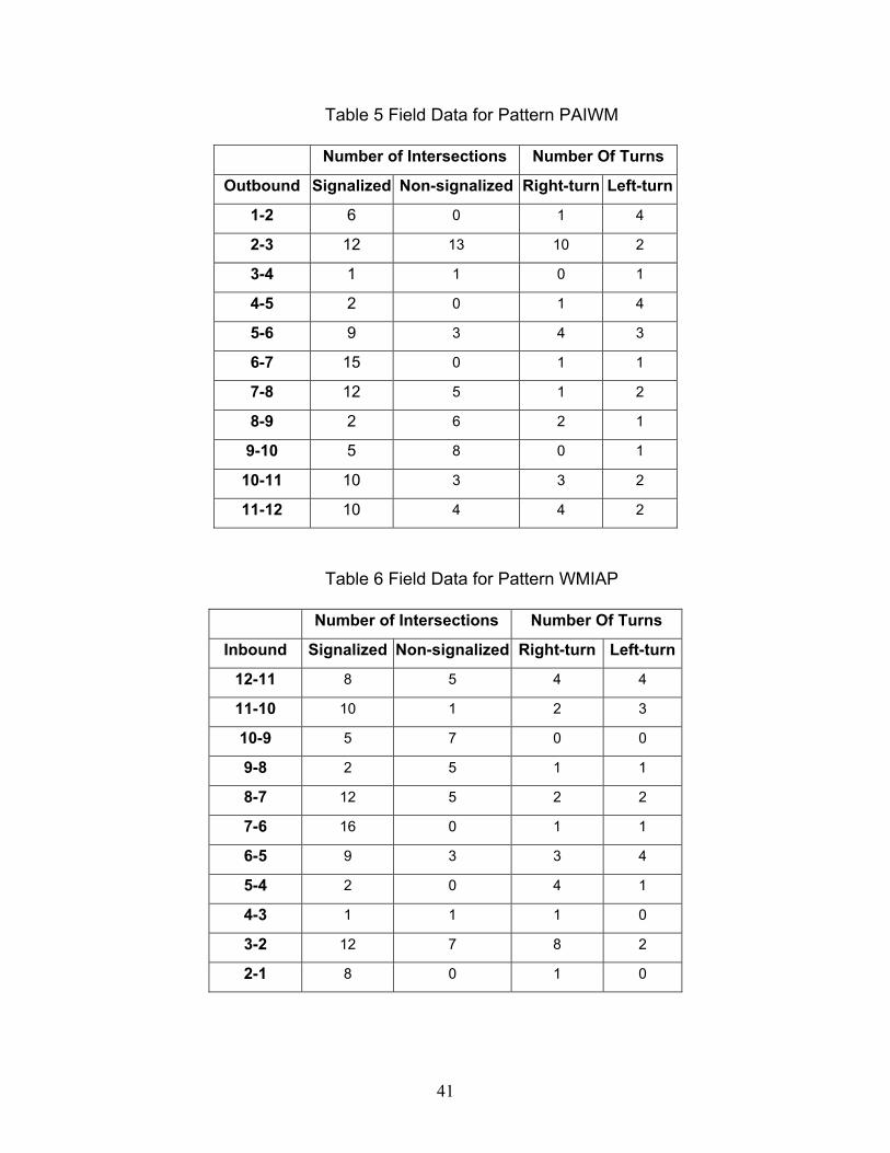
Table 5 Field Data for Pattern PAIWM
Number of Intersections Number Of Turns
Outbound Signalized Non-signalized Right-turn Left-turn
1-2 6 0 1 4
2-3 12 13 10 2
3-4 1 1 0 1
4-5 2 0 1 4
5-6 9 3 4 3
6-7 15 0 1 1
7-8 12 5 1 2
8-9 2 6 2 1
9-10 5 8 0 1
10-11 10 3 3 2
11-12 10 4 4 2
Table 6 Field Data for Pattern WMIAP
Number of Intersections Number Of Turns
Inbound Signalized Non-signalized Right-turn Left-turn
12-11 8 5 4 4
11-10 10 1 2 3
10-9 5 7 0 0
9-8 2 5 1 1
8-7 12 5 2 2
7-6 16 0 1 1
6-5 9 3 3 4
5-4 2 0 4 1
4-3 1 1 1 0
3-2 12 7 8 2
2-1 8 0 1 0
41
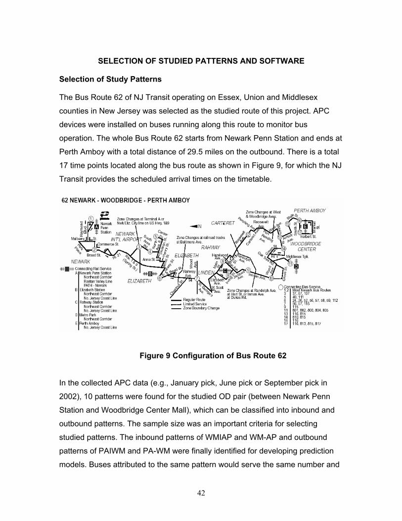
SELECTION OF STUDIED PATTERNS AND SOFTWARE
Selection of Study Patterns The Bus Route 62 of NJ Transit operating on Essex, Union and Middlesex
counties in New Jersey was selected as the studied route of this project. APC
devices were installed on buses running along this route to monitor bus
operation. The whole Bus Route 62 starts from Newark Penn Station and ends at
Perth Amboy with a total distance of 29.5 miles on the outbound. There is a total
17 time points located along the bus route as shown in Figure 9, for which the NJ
Transit provides the scheduled arrival times on the timetable.
Figure 9 Configuration of Bus Route 62 In the collected APC data (e.g., January pick, June pick or September pick in
2002), 10 patterns were found for the studied OD pair (between Newark Penn
Station and Woodbridge Center Mall), which can be classified into inbound and
outbound patterns. The sample size was an important criteria for selecting
studied patterns. The inbound patterns of WMIAP and WM-AP and outbound
patterns of PAIWM and PA-WM were finally identified for developing prediction
models. Buses attributed to the same pattern would serve the same number and
42

sequence of time points. The time point sequence for studied patterns are listed
in Tables 7, 8, 9, and 10. The GIS diagram of the studied patterns is shown in
Figure 10.
Table 7 Time Points for Pattern WMIAP (inbound)
Time Point Description Distance to Start Point (mi)
WOODBRIDGE CENTER MALL 0.00 NJT METROPARK STATION 3.77 INMAN AVE & WOOD AVE 7.14
W INMAN AVE & ST GEORGES AVE 9.67 MAIN ST & E MILTON AVE 10.81
SAINT GEORGES AVE & WOOD AVE 13.74 E JERSEY ST & BROAD ST 17.30
IKEA 21.06 FEDERAL EXPRESS - NEWARK AIRPORT 23.16
NWK AIRPORT TERM A 24.05 NWK AIRPORT TERM B 24.65 NWK AIRPORT TERM C 25.15 BROAD ST & EDISON PL 28.97
PENN STATION BUS LANES 29.63
43

Table 8 Sequence of Time Points for Pattern PAIWM (outbound) Time Point Description Distance to Start Point (mi)
PENN STATION BUS LANES 0 BROAD ST & BRANFORD PL 0.76
NWK AIRPORT TERM A 4.56 NWK AIRPORT TERM B 5.01 NWK AIRPORT TERM C 5.52
FEDERAL EXPRESS - NEWARK AIRPORT 7.70 IKEA 9.78
BROAD ST & W JERSEY ST 13.74 SAINT GEORGES AVE & WOOD AVE 17.16
IRVING ST & BROAD ST 19.94 W INMAN AVE & ST GEORGES AVE 21.13
INMAN AVE & WOOD AVE 23.66 NJT METROPARK STATION 26.86
WOODBRIDGE CENTER MALL 30.03
Table 9 Time Points for Pattern WM-AP (inbound) Time Point Description Distance to Start Point (mi)
WOODBRIDGE CENTER MALL 0.00 NJT METROPARK STATION 3.77 INMAN AVE & WOOD AVE 7.14
W INMAN AVE & ST GEORGES AVE 9.67 MAIN ST & E MILTON AVE 10.81
SAINT GEORGES AVE & WOOD AVE 13.74 E JERSEY ST & BROAD ST 17.30
NWK AIRPORT TERM A 20.86 NWK AIRPORT TERM B 21.30 NWK AIRPORT TERM C 21.81 BROAD ST & EDISON PL 25.70
PENN STATION BUS LANES 26.37
44

Table 10 Time Points for Pattern PA-WM (outbound)
Time Point Description Distance to Start Point (mi)
PENN STATION BUS LANES 0.00
BROAD ST & BRANFORD PL 3.77
NWK AIRPORT TERM A 7.14
NWK AIRPORT TERM B 9.67
NWK AIRPORT TERM C 10.81
BROAD ST & W JERSEY ST 13.74
SAINT GEORGES AVE & WOOD AVE 17.30
IRVING ST & BROAD ST 20.86
W INMAN AVE & ST GEORGES AVE 21.30
INMAN AVE & WOOD AVE 21.81
NJT METROPARK STATION 25.70
WOODBRIDGE CENTER MALL 26.37
Study Pattern (PennStation-Woodbridge Mall)
Figure 10 The Studied Patterns in GIS
45

Selection of Software As mentioned earlier, the objective of this study is to develop a neural dynamic
model for bus travel time prediction. The research team applied a well-developed
commercial software to form the proposed model.
Among various software packages, NeuroSolutions was selected because it is at
the leading edge of neural network simulation technology. Using an object-
oriented approach, NeuroSolutions allows user to create an artificial neural
network (ANN) that is composed of individually simple components. The network
can be built through an icon-based design interface, which provides much more
flexibility than a typical “black box” simulator. NeuroSolutions is capable of
generating powerful ANNs to solve complicated problems. A unique feature of
the software is that it contains a comprehensive collection of probes that allows
the user/designer to monitor every aspect of the ANN during training and testing.
NeuroSolutions is one of the few products on the market that is able to handle all
four types of problems: (1) classification, (2) function approximation, (3)
prediction, and (4) clustering. There are six different levels of the software: (1)
educator, (2) users, (3) consultants, (4) professional, (5) developers lite, and (6)
developers. The level used in this study is “users-level”.
NeuroSolutions has two separated wizards, NeuralExpert and NeuralBuilder, that
one can use to automatically build an ANN to the design specification. The
NeuralExpert centers the design specification around the type of problem one
wish to solve. Based on this and the size of the data, it can intelligently select
the size and architecture of the ANN that will produce a good solution. The
NeuralBuilder centers the design around the specific ANN architecture that one
wish to build. The network parameters such as the number of hidden layers, the
number of processing elements, and the learning algorithm can be customized.
In addition, genetic algorithm is available to optimize these parameter settings at
the user/designer’s choice.
46
DATA PROCESSING Data Screening There were many indices recorded in the APC dataset for each bus trip. Records
that were missing or incorrect in the raw data file were identified and removed
from the database. Different problems experienced while processing the APC
data were itemized below as well as the corresponding solutions.
The problems experienced in APC data:
• Duplicated records.
• Wrong start or end position.
• Unreasonable arrival time along stops.
• Missing data.
• Inconsistent data (e.g., open vs. close time, scheduled vs. actual
running time).
• Times are recorded in different format (e.g., hour/minute/second,
minutes).
The corresponding solutions to the above problem:
• Delete duplicated records.
• Adjust start or end position.
• Use actually arrival time at time points to interpolate the appropriate
arrival.
• Use speed and distance information to derive travel time.
• Correct the wrong information.
• Unify the format of all time indices.
Data Calculation APC devices installed in buses can record the numbers of boarding and alighting
passengers when bus doors were opened to serve passengers. Therefore, there
47

was no record for the skipped time points. The cumulative numbers of boarding
and alighting passengers and dwell times at stops were calculated for those
missing time points. In order to provide sufficient data to develop proposed
prediction models, the completed cumulative numbers of boarding and alighting
passengers and dwell times at all time points are also generated.
Data Interpolation The ideal data structure for observing bus operations is a set of successive time
point records. Thus, the actual bus travel times between time points can be
compared with that posted on the timetable. However, in the APC dataset, some
records were missing because buses skipped the time points where there was no
demand at that time. In order to generate a completed time point to time point
(TP-to-TP) information, the missing data at some TPs were approximated based
on the available information at adjacent TP.
An interpolation algorithm is developed to derive arrival time for the skipped time
points based on the previous and next time point records. Though the bus arrival
times of the skipped time points can be obtained by assuming the bus operated
with a constant speed between two several time points, other information such as
dwell time and number of boarding passengers are still unavailable. Thus, the
actual dwell times and number of boarding passenger information at the skipped
TPs were obtained similarly.
The ideal data structure should include all the time points in sequence for each
trip. As mentioned earlier, in the APC data, records at skipped time points were
unavailable and then an interpolation is needed to approximate bus arrival
information. The interpolation was illustrated as follows:
48

O A B
D
Let
Arri
‘A’ a
‘A’ a
Let
All t
the
Thu
s =
whe
inte
Tab
Fina
A, B, and C be assume
val time at time point ‘B
nd the interpolated tra
nd ‘C’.
Da = Distance of tim
Db = Distance of tim
Dc = Distance of tim
he distances between
following information c
Ta = Leg time of ‘A’
Tab = Leg time of ‘B
Tac = Leg time of ‘C
s, the average speed f
(Dc – Da)/ Tac
re (Dc – Da) represent
rpolated travel time can
= (Db – Da)/ s
lly, the bus arrival time
d time points, where time poin
’ can be computed by adding d
vel time of link AB based on ar
e-point ‘A’ from the origin
e-point ‘B’ from the origin
e-point ‘C’ from the origin
time points are provided from N
an be obtained from APC data
from the preceding time point (
’ from ‘A’
’ from ‘A’
rom A to D can be obtained fro
the travel distance from A to D
be estimated by applying Equ
at ‘B’ would be door close tim
49
t ‘B’ was skipped.
oor close time at
rival times at time
J Transit. In addit
.
=0 for the first sto
m Equation (1).
. Therefore, the
ation (2).
e at ‘A’ plus Tab
Da
Db
Dc
stop
points
ion,
p)
(1)
(2)

Summary After processing the original APC dataset, the calculated data and interpolated
data need to be merged with the weather data as one dataset for developing
prediction models. The unique index was chosen between two different datasets.
For example, “month/date/hour” could be used to merge weather data with the
APC data, and “month/date/pattern/tripID” could be used as the unique index to
merge calculated data (e.g., cumulative boarding and alighting passenger at
each stop) with the original APC data. After merging the collected data including
bus arrival times and numbers of boarding and alighting passengers at all time
points, weather information, and accumulated dwell times between pairs of time
points were processed and ready for developing the proposed predictive models.
50
MODEL DEVELOPMENT
Introduction As the primary form of public transit, bus service operates on urban streets with
shared right-of-way with automobiles and commercial vehicles and trucks. As a
result, the service reliability of bus transit could be greatly compromised by
various unexpected incidents along its route. This also leads to inaccurate or
unreliable arrival times, which incur a long and unpredictable wait time
experienced by transit users.
Advanced sensing, positioning, and communication technologies have provided
a good platform to obtain reliable information on transit vehicle trip information.
The Advanced Passenger Counter (APC) system deployed by New Jersey
Transit on its partial fleet has been generating such information everyday. This
includes bus trip activities such as stop, door open/close, number of passengers
boarding/alighting at each stop, and the associated temporal (e.g., time) and
spatial (e.g., latitude) information. In addition, the ridership information that is
usually expensive to obtain with traditional methods and is extremely valuable in
estimating bus arrival times at downstream stops can be collected.
In this chapter, a methodology that has been developed to predict transit vehicle
arrival times using data generated by APC devices installed on buses operated
by New Jersey Transit is presented next.
Artificial Neural Networks (ANNs)
ANN modeling techniques have been of great interest to many researchers. The
advantage of this technique is that it is unnecessary to assume a functional form
between the dependent and independent variables. This is extremely useful
when the data display non-linear relationship.
51
Using ANNs in forecasting has become more popular in transportation research.
Related studies include Hua and Faghri (32), Chin et al. (33), Dougherty (34),
Kalaputatu and Demetsky (35), Smith and Demetsky (36), Zhang et al. (37), Chang
and Su (38), Wei and Yang (39), and Ding and Chien (40) Designed with versatile
parallel distributed structures and adaptive learning processes, the ANN is
considered as a promising approach to describe complex systems such as transit
operation that is affected by various inter-correlated and time varying factors.
Unlike other prediction models, the ANN does not require a specific form of
function. This eliminates the need of function development and parameter
estimation for nonlinear and time varying systems. A well-trained ANN could
capture complex relationship between the dependent variables (output such as
bus arrival time) and a set of explanatory/independent variables (input such as
traffic conditions and passenger demand) (40). Therefore, the ANN technique
could be very useful in prediction when it is difficult or even impossible to
mathematically formulate the relationship between the input and output.
However, the extent to which an ANN is trained could have significant impact on
its prediction performance, especially in some applications where only small
amount of data is available for training.
ANN Basics
The ANN is a network consisting of interconnected units called processing
elements (PEs, also known as artificial neurons because it has certain
resemblance to the neurons in the human brain). Each PE receives connections
from other PEs and/or itself. The signals transmitted through the connections are
scaled by adjustable parameters called weights. A weight is associated with
every connection in the network.
In this study, we are exploring the relationship between bus travel times and
various inputs such as time of the day, day of the week, and weather
52

(precipitation). Therefore, the ANN should be designed to solve problem with
function approximation type.
The multilayer perceptron (MLP) typed ANN architecture was chosen since it is
generally easy to use and can approximate almost any input/output map. It has
been widely used in countless applications. Its major disadvantages include slow
training process and high demand on data amount. A typical MLP architecture
with one hidden layer is shown Figure 11.
Figure 11 MLP with One Hidden Layer Back-propagation is the most commonly used algorithm in training an ANN (41). A
back-propagation network (BPN) is trained in a supervised mode, i.e., the
weights of the network is continually adjusted to incrementally reduce the
difference between the output of the system and the desired response. Its
general procedure is shown in Figure 12 (42). For a single layer network,
corrections are made for the weights in proportion to the error between the
desired output (e.g., actual travel time) and the network output (e.g., predicted
travel time). For a multiple-layer ANN, corrections have to be made for the
weights from the first to the second layer, the second to the third layer, and so
on. The stopping criterion could be a pre-set number of iterations, a specific
output mean square error (MSE), or cross validation that is the most powerful
one among them.
53
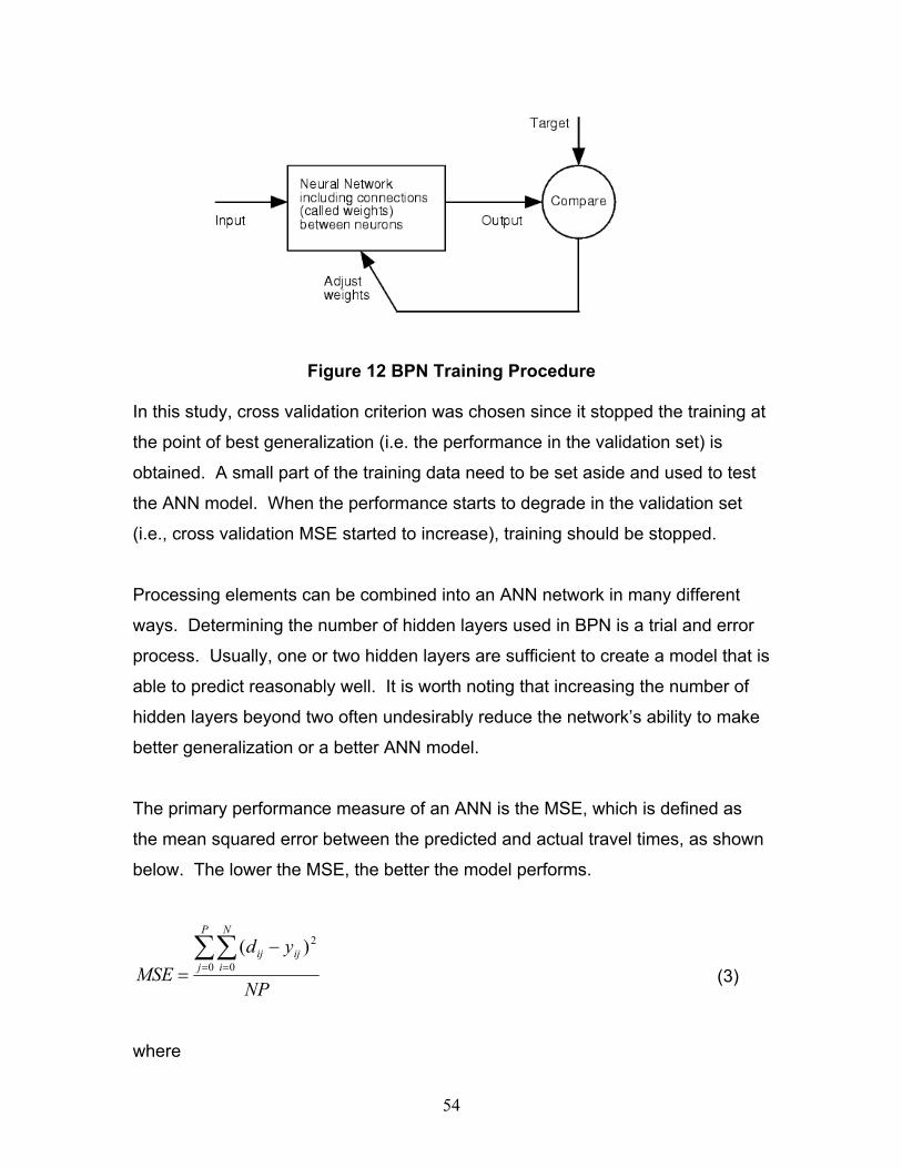
Figure 12 BPN Training Procedure In this study, cross validation criterion was chosen since it stopped the training at
the point of best generalization (i.e. the performance in the validation set) is
obtained. A small part of the training data need to be set aside and used to test
the ANN model. When the performance starts to degrade in the validation set
(i.e., cross validation MSE started to increase), training should be stopped.
Processing elements can be combined into an ANN network in many different
ways. Determining the number of hidden layers used in BPN is a trial and error
process. Usually, one or two hidden layers are sufficient to create a model that is
able to predict reasonably well. It is worth noting that increasing the number of
hidden layers beyond two often undesirably reduce the network’s ability to make
better generalization or a better ANN model.
The primary performance measure of an ANN is the MSE, which is defined as
the mean squared error between the predicted and actual travel times, as shown
below. The lower the MSE, the better the model performs.
NP
ydMSE
P
j
N
iijij∑∑
= =
−= 0 0
2)( (3)
where
54

=P number of output neurons
=N number of samples in the data set
ijd =desired output for sample at neuron i j
=ijy network output for sample i at neuron j
Other performance measures include normalized mean squared error, percent
error, etc.
Applicability Using ANNs has an advantage over conventional prediction methods for it can
handle complicated systems that are hard to formulate. Unlike regression, which
needs an explicitly defined function to relate the input and the output, the ANN
can approximate a function and associate input with specific output after being
properly trained. This capability is extremely useful when the system is rather
complex (such as transit operation) and/or it is impossible to specify a form of
function to accurately represent the relationship between the input and output.
Moreover, an ANN does not require input variables to be independent with each
other, which could save substantial effort in data correlation analysis.
Data Requirement To model an ANN, a large amount of data would be required. A general “rule of
thumb” is that the number of exemples (training data records) should be at least
three times of the number of network weights. The number of network weights
can be adjusted via a number of approaches, such as reducing the number of
hidden layers, reducing the number of processing elements (PEs) in each hidden
layer, applying weight decay when using full synapse between layers, or
choosing arbitrary synapse over full synapse. Currently, the amount of data that
is usable in ANN modeling is relatively small. Therefore, reducing the number of
weights in the network was used to satisfy the aforementioned data ratio. In
55

addition, due to the limited data amount, the number of hidden layers is restricted
to one.
However, the research team believes that with new APC data being added to the
central database everyday, the data amount requirement can be satisfied
eventually without applying those weight reduction measures.
Pre-Processing Input and Output The studied APC data provided by NJ Transit included a total of four different
patterns on both service directions (inbound and outbound). The selected
patterns are WMIAP, PAIWM, WM-AP, and PA-WM as described in Section 4.1.
For each direction, there are 12 and 14 time points for patterns (PA-WM, WM-
AP) and (PAIWM, WMIAP) respectively. Therefore, the prediction of bus arrival
times for the four patterns need to be modeled separately.
Among those variables that may contribute to the variation of bus travel time
between time points, the research team selected the following as the weight
parameters: time of the day, day of the week, and weather (e.g., precipitation).
The output of the model will be the travel times on each segment of the route,
i.e., between two consecutive time points. Then the arrival time can be calculated
based on the departure time from previous time point and the estimated travel
time to the subject time point.
Data Format NeuroSolutions requires that all input files be saved as a coma delimited text file.
Each trip in the data file would occupy one row in which travel time between time
points, as well as time of the day, day of the week, and weather information are
selected. All trips belonging to the same pattern for each direction are located in
56

one input file. For the purpose of calculation convenience, the travel time has
been converted to the number of seconds. A sample data file is shown in Figure
13.
Mo In
AN
ne
pr
St
St
St
St
St
St
St
Figure 13 Sample Data File
deling Procedure
this study, the NeuralExpert tool of NeuroSolutions was used to develop
Ns. It is a wizard that asks user questions and automatically builds the best
twork and configures the parameters and probes for the problem. The general
ocedure is outlined as follows.
ep 1: Identify the problem type as function approximation.
ep 2: Identify the input file.
ep 3: Specify input variables (e.g., time of the day, day of the week, and
precipitation).
ep 4: Tag symbolic inputs. Due to the nature of the input variables in the study
as symbolic rather than numerical values that is continuous, it is
necessary to specify that all three variables are symbolic.
ep 5: Identify the file that contains data to model. This is the same as the input
file based on the way we process data. Therefore, choose “use input file
for desired file” and “shuffle data files” to randomize the file order.
ep 6: Select the columns to model, i.e., select those travel times, which are
labeled, from TT1 to TT11 (for the patterns with 12 time points) or up to
TT13 (for the patterns with 14 time points).
ep 7: Choose a level of generalization protection. This is to help the ANN
perform better on new data in the training process. It is implemented by
setting aside data used to determine when to stop training the ANN
57

(called cross validation data set). Normal level with 20 percent cross
validation data from the input file was chosen.
Step 8: Choose “out of sample testing”, i.e., set aside certain percentage of
samples from the input file to test the ANN after training and cross
validation. Due to limited size of samples, 3 percent was specified.
Step 9: Specify level of genetic optimization (e.g., “None”). Performing genetic
optimization involves using large amount of data.
Step 10: Choose the level of neural network complexity as “Low”. This will
establish an ANN with one hidden layer, which is preferred due to limited
size of training data.
The wizard is likely to send a warning for the shortage of data afterwards. This
problem can be dealt with additional adjustments as follows. The purpose of this
procedure is to reduce the number of connections in the network, aiming to
reduce the number of network weights.
Step 1: Check the weight decay box on the momentum inspectors associated
with the synapses between the input and hidden layers and between the
hidden and output layers. The default weight decay rate is 0.01.
Step 2: Add weight inspectors on these two synapses and show the weights
during the training process.
Step 3: Train the ANN using different weight decay rate, and save the one with
the best MSEs.
Step 4: Based on weights in the weight inspector, change full synapse to
arbitrary synapse. Connect the PEs with input and output variables if the
weight is high in absolute value.
Step 5: Calculate the number of network weights by adding number of weights
from synapses between input and hidden layer and between hidden and
output layer, and weights from the hidden layer. The number of weights
for the synapses can be found from the Soma tab of the synapse
inspector, while that for the hidden layer can be found from the Soma tab
58

of the TahnAxon inspector. The total number of training samples should
be at least 3 times of the number of network weights.
ANN Models Four ANN models were established in this study to predict bus travel time by
pattern and by direction, as shown in Table 11.
Table 11 Developed ANN Models Inbound Outbound
Patterns (w/ 12 time points) Model I (for WM-AP) Model II (for PA-WM)
Patterns (w/ 14 time points) Model III (for WMIAP) Model IV (for PAIWM)
Model I The network architecture shown in Figure 14 presents the elements in the ANN
that have been addressed on the documentation of NeuroSolutions.
axon
Figure 14 Network Architecture of Model I The axon at the far left side is the input layer. It is connected with a hidden layer
through a TahnAxon type transfer function and hidden synapse with 11 weights.
There are 3 PEs in the hidden layer, which is connected to the output layer
through output synapse with 11 weights. Therefore the total number of weights
for this network is 25. The total number of data samples is 81, while 20 percent
of these (16 samples) were used in cross validation, and 2 samples were used in
testing. The training data file then has 63 samples. This number of samples is
low compared to the recommended sample size (3 times of the total network
59

weights). However, in order to evaluate all input variables, the network weights
cannot be further reduced.
After the network has been established, multiple trainings were conducted and
the best one (with the minimum MSE) was saved. Figure 15 shows the learning
curve of the training process. The horizontal axis represents the number of
epochs (i.e., the number of times that training data is presented to the network),
while the vertical axis represents the MSE and the horizontal axis represents the
number of iterations. It can be observed that the learning curve is rather smooth
which indicates that the model performance is steadily improving even though
very slowly after 200 iterations.
The network weights as generated by the software are shown in Table 12 as the
output of the sensitivity analysis. Since all input variables in the study are
symbolic type variables, they were split into multiple subvariables in the network.
Figure 15 Learning Curves of Model I
60

Table 12 Values of Parameters in Model I Input Variable Weight Cumulative Weight
Monday 0.14 Tuesday 4.33
Wednesday 1.91 Thursday 1.75
Day of the Week
Friday 4.18
12.32
MP 5.91 AP 18.12 E 15.78
Time of the Day
LN 41.34
81.14
Precipitation – N 3.26 Precipitation Precipitation – Y 3.28 6.54
To evaluate the impact of the each variable, one can add the weights of all
subvariables that belong to one original variable. For example, one should add
weights for all days of a week to obtain the impact of day of the week on bus
travel times. The cumulative significance of each variable is also shown in Table
12, from which one can observe that “time of the day” is the most significant
factor in affecting bus travel times. Compared to “time of the day”, “day of the
week” and “precipitation” do not have such significant impact.
Model II
The network architecture for Model II is similar to that of Model I as shown in
Figure 14. The total number of data samples is 112, with which 22 samples (20
percent) were used for cross validation and 3 samples were used for testing.
This leaves the number of training samples to be 89. The total number of
network weights is 25, with 11, 3, and 11 weights at the hidden synapse, hidden
layer, and output synapse, respectively. Therefore the training sample size can
satisfy the recommended level.
The learning curve is shown in Figure 16, and the results of the sensitivity
analysis are shown in Table 13. Similar to Model I, the training process seems to
61

be smooth, and “time of the day” is the most significant one among all three input
variables.
Figure 16 Learning Curves of Model II
Table 13 Values of Parameters in Model II Input Variable Weight Cumulative Weight
Monday 2.22 Tuesday 2.88
Wednesday 0.33 Thursday 4.64
Day of the Week
Friday 0.63
10.70
EM 18.05 MP 22.23 AP 18.32
Time of the Day
E 22.19
80.79
Precipitation – N 4.25 Precipitation Precipitation – Y 4.26 8.51
Model III Model III was developed for the inbound pattern with 14 time points traveling
inbound (WMIAP). Its network architecture remains similar to that of Models I and
II, as shown in Figure 14.
62

The total number of data samples is 135, among them 27 samples (20 percent)
were used for cross validation and 4 samples were used for testing. This leaves
the number of training samples to be 104. The total number of network weights
is 29, with 13, 3, and 13 weights at the hidden synapse, hidden layer, and output
synapse, respectively. Thus, the training sample size can satisfy the
recommended level.
The learning curve for Model III is shown in Figure 17, and the results of the
sensitivity analysis is shown in Table 14. Similar to Models I and II, the training
process seems to be smooth, and “time of the day” is the most significant one
among all three input variables.
Figure 17 Learning Curves of Model III
63

Table 14 Values of Parameters in Model III Input Variable Weight Cumulative Weight
Monday 0.01 Tuesday 0.75
Wednesday 2.61 Thursday 0.08
Day of the Week
Friday 1.46
4.90
EM 22.50 LM 4.55 MD 10.73 EA 15.02 E 13.34
Time of the Day
LN 25.34
91.49
Precipitation – N 1.80 Precipitation Precipitation – Y 1.81 3.61
Model IV Model IV was developed for the outbound pattern serving 14 time points
(PAIWM). Its network architecture remains similar to that of models I, II, and III,
as shown in Figure 14.
The total number of data samples is 121, among them 24 samples (20 percent)
were used for cross validation and 4 samples were used for testing. This leaves
the number of training samples to be 93. The total number of network weights is
29, with 13, 3, and 13 weights at the hidden synapse, hidden layer, and output
synapse, respectively. Therefore, the training sample size can satisfy the
recommended level.
The learning curve for Model IV is shown in Figure 18, and the results of the
sensitivity analysis is shown in Table 15. Similar to Models I, II, and III, the
training process seems to be smooth, and “time of the day” is the most significant
one among all three input variables.
64

Figure 18 Learning Curves of Model IV
Table 15 Values of Parameters in Model IV Input Variable Weight Cumulative Weight
Monday 2.94 Tuesday 2.12
Wednesday 0.76 Thursday 1.75
Day of the Week
Friday 2.84
10.41
EM 26.04 LM 3.89 MD 1.57 EA 25.49 AP 14.10
Time of the Day
E 16.94
88.02
Precipitation – N 0.78 Precipitation Precipitation – Y 0.78 1.57
Kalman Filtering Algorithm The ANNs developed in this study are based on historic data pool of bus trips.
New data are added into that pool regularly. Training can then be conducted
afterwards to ensure the ANN models up to date. However, this method does not
have the dynamic feature to adapt to incident (non-recurring) condition.
65

A dynamic procedure was developed based on the Kalman filtering algorithm. It
enables online adjustment of arrival time estimates for a particular trip based on
its available travel time information up to the moment the estimation is
conducted.
Let t denote the travel time from time point to the given destination (i.e., the
time point for which arrival time prediction is performed), T denote the travel
time from time point to time point
k k
1, +kk
k 1+k , denote the travel time from origin to
time point . Then the travel time from time point
ks
k 1+k to the destination t can
be calculated as t , and the travel time from origin to time point
1+k
1,1 ++ − kkkk Tt= 1+k
can be calculated as 1, +1+ += kk s kkTs .
If denotes the observed travel time from origin to time point , then .
Let , the Kalman filter can be formulated as
kz
x
k kk sz =
( Tkkk st= )
kkkkk wAxx ++Φ=+1 (4)
kkkk vxHz += (5)
in which,
=Φ
1001
k
, , ( )10=kH
−=
+
+
1,
1,
kk
kkk T
TA
kw and are white noises associated with the transition process and
measurement, respectively. They are assumed to have zero mean and
variances of Q and , respectively.
kv
k kR
The filtering procedure is outlined as follows.
66

Step 1: Initialize state variables. Set ( )Tstx 000= , in which is the estimated
total travel time from the origin to the destination, and is set to be 0
based on its definition.
0t
0s
Step 2: Initialize covariance when 0P 0=k .
Step 3: State variable extrapolation.
(6)
in which T can be obtained from estimates based on historical data.
−+
=+Φ=
+
++
−+
1,
1,11 10
01ˆ
kk
kk
k
kkkkk T
Tst
Axx
1, +kk
Step 4: Covariance extrapolation.
(7) kTkkkk QPP +ΦΦ= ++
−+ 111
Step 5: Kalman gain computation.
(8) ( ) 11111111
−
++−+++
−++ += k
Tkkk
Tkkk RHPHHPK
Step 6: State variable update.
( )−++++
−++ −+= 111111 ˆˆˆ kkkkkk xHzKxx
1+
(9)
Stop, if time point k is the destination. Otherwise, go to Step 7.
Step 7: Covariance update.
(10)
Go to Step 3.
−+++
−++ −= 11111 kkkkk PHKPP
67
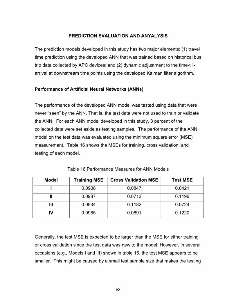
PREDICTION EVALUATION AND ANYALYSIS
The prediction models developed in this study has two major elements: (1) travel
time prediction using the developed ANN that was trained based on historical bus
trip data collected by APC devices; and (2) dynamic adjustment to the time-till-
arrival at downstream time points using the developed Kalman filter algorithm.
Performance of Artificial Neural Networks (ANNs)
The performance of the developed ANN model was tested using data that were
never “seen” by the ANN. That is, the test data were not used to train or validate
the ANN. For each ANN model developed in this study, 3 percent of the
collected data were set aside as testing samples. The performance of the ANN
model on the test data was evaluated using the minimum square error (MSE)
measurement. Table 16 shows the MSEs for training, cross validation, and
testing of each model.
Table 16 Performance Measures for ANN Models
Model Training MSE Cross Validation MSE Test MSE
I 0.0908 0.0847 0.0421
II 0.0987 0.0712 0.1196
III 0.0934 0.1182 0.0724
IV 0.0985 0.0891 0.1220
Generally, the test MSE is expected to be larger than the MSE for either training
or cross validation since the test data was new to the model. However, in several
occasions (e.g., Models I and III) shown in table 16, the test MSE appears to be
smaller. This might be caused by a small test sample size that makes the testing
68

result relatively volatile. However, with the increase of testing samples in the data
pool, the model performance shall be more stable.
During the process of ANN model development in this study, only a small amount
of samples (3 percent) were applied as testing data. The recommended minimum
ratio of training samples to network weights that is 3, was not sufficient even with
such a small data was selected for testing the ANN. To evaluate the performance
of the model, all data were used in the test process. The variation between
scheduled and actual travel times and the variation between the predicted (ANN
output) and actual travel times were compared.
Figures 19 through 26 show the spatial and temporal variations of prediction
errors with all four ANN models. The average errors in these figures are
calculated using Eqs. 11 and 12.
a
aANNANN t
tte −= (11)
Accordingly, the error between the scheduled and actual travel times can be
found as:
a
aSS t
tte
−= (12)
where eANN: Prediction error from the ANN
tANN: Predicted travel time from the ANN
eS: Prediction error of scheduled travel time
tS: Scheduled travel time from the timetable
ta: Actual travel time
69

0
5
10
15
20
25
30
35
1-2 2-3 3-4 4-5 5-6 6-7 7-8 8-9 9-10 10-11 11-12
TP-TP
Ave
rrag
e Er
ror (
%)
Predicted Travel Time (ANN) Scheduled Travel Time
TP # Description
1 WOODBRIDGE CENTER MALL
2 NJT METROPARK STATION
3 INMAN AVE & WOOD AVE
4 W INMAN AVE & ST GEORGES AVE
5 MAIN ST & E MILTON AVE
6 SAINT GEORGES AVE & WOOD AVE
7 E JERSEY ST & BROAD ST
8 NWK AIRPORT TERM A
9 NWK AIRPORT TERM B
10 NWK AIRPORT TERM C
11 BROAD ST & EDISON PL
12 PENN STATION BUS LANES
Figure 19 Predicted (Model I) vs. Scheduled Errors for TP-to-TP Travel Times
0
5
10
15
20
25
30
35
MP AP E LN
Time of the Day
Ave
rage
Err
or (
%)
Predicted Travel Time (ANN) Scheduled Travel Time
Figure 20 Predicted (Model I) vs. Scheduled Errors for
Travel Times in Different Periods
70
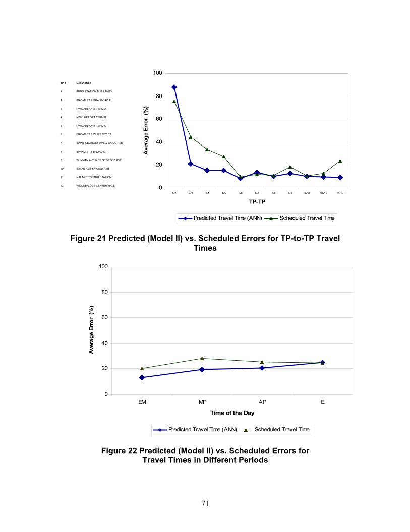
TP # Description
1 PENN STATION BUS LANES
2 BROAD ST & BRANFORD PL
3 NWK AIRPORT TERM A
4 NWK AIRPORT TERM B
5 NWK AIRPORT TERM C
6 BROAD ST & W JERSEY ST
7 SAINT GEORGES AVE & WOOD AVE
8 IRVING ST & BROAD ST
9 W INMAN AVE & ST GEORGES AVE
10 INMAN AVE & WOOD AVE
11 NJT METROPARK STATION
12 WOODBRIDGE CENTER MALL
0
20
40
60
80
100
1-2 2-3 3-4 4-5 5-6 6-7 7-8 8-9 9-10 10-11 11-12
TP-TP
Ave
rage
Err
or (
%)
Predicted Travel Time (ANN) Scheduled Travel Time
Figure 21 Predicted (Model II) vs. Scheduled Errors for TP-to-TP Travel Times
0
20
40
60
80
100
EM MP AP E
Time of the Day
Ave
rage
Err
or (
%)
Predicted Travel Time (ANN) Scheduled Travel Time
Figure 22 Predicted (Model II) vs. Scheduled Errors for Travel Times in Different Periods
71

TP # Description
1 WOODBRIDGE CENTER MALL
2 NJT METROPARK STATION
3 INMAN AVE & WOOD AVE
4 W INMAN AVE & ST GEORGES AVE
5 MAIN ST & E MILTON AVE
6 SAINT GEORGES AVE & WOOD AVE
7 E JERSEY ST & BROAD ST
8 IKEA
9 FEDERAL EXPRESS - NEWARK AIRPORT
10 NWK AIRPORT TERM A
11 NWK AIRPORT TERM B
12 NWK AIRPORT TERM C
13 BROAD ST & EDISON PL
14 PENN STATION BUS LANES
0
10
20
30
40
1-2 2-3 3-4 4-5 5-6 6-7 7-8 8-9 9-10 10-11 11-12 12-13 13-14
TP-TP
Ave
rage
Err
or (%
)
Predicted Travel Time (ANN) Scheduled Travel Time
Figure 23 Predicted (Model III) vs. Scheduled Errors for TP-to-TP Travel Times
0
10
20
30
40
EM LM MD EA E LN
Time of the Day
Ave
rage
Err
or (
%)
Predicted Travel Time (ANN) Scheduled Travel Time
Figure 24 Predicted (Model III) vs. Scheduled Errors for Travel Times in Different Periods
72

TP # Description
1 PENN STATION BUS LANES
2 BROAD ST & BRANFORD PL
3 NWK AIRPORT TERM A
4 NWK AIRPORT TERM B
5 NWK AIRPORT TERM C
6 FEDERAL EXPRESS - NEWARK AIRPORT
7 IKEA
8 BROAD ST & W JERSEY ST
9 SAINT GEORGES AVE & WOOD AVE
10 IRVING ST & BROAD ST
11 W INMAN AVE & ST GEORGES AVE
12 INMAN AVE & WOOD AVE
13 NJT METROPARK STATION
14 WOODBRIDGE CENTER MALL
3
Figure 25 Predicted (Model IV) vs. Scheduled Errors for TP-to-TP Travel Times
0
20
40
60
80
1-2 2-3 -4 4-5 5-6 6-7 7-8 8-9 9-10 10-11 11-12 12-13 13-14
Route Segment
Ave
rage
Err
or (
%)
Predicted Travel Time (ANN) Scheduled Travel Time
0
20
40
60
80
EM LM MD EA AP E
Time of the Day
Ave
rage
Err
or (
%)
Predicted Travel Time (ANN) Scheduled Travel Time
Figure 26 Predicted (Model IV) vs. Scheduled Errors for
Travel Times in Different Periods
73
It was observed that, the ANN gave in general a better estimate of the travel time
than that from the timetable since the average error of ANNs in most cases is
less than that from the timetable. However, in a few cases, the timetable
estimates were better than that from the ANNs. This might be attributable to two
facts: (1) the limited available data for ANN model development; and (2) the error
in original APC data.
Even though the stability of the ANN prediction was affected by the quality and
quantity of the data, the research team believes that with more new data added
into the APC database, the performance of the neural network models shall be
further improved.
Performance of the Neural/Dynamic (N/D) Model In this study, a neural/dynamic (N/D) model that integrates the Kalman filtering
algorithm and an ANN was developed to dynamically adjust the predicted bus
arrival time. Whenever a bus reaches a time point, the travel/arrival time
prediction from a corresponding ANN can be adjusted according to real time
information (e.g., the most updated travel/arrival times).
The estimated travel time to each downstream time point was updated when the
most recent bus arrival information became available. For example, as a bus
departs from time point 1, the ANN predicts the arrival times from first time point
to all downstream time points. When the bus arrives at time point 2, the new
prediction is based on the Kalman filter, while the prediction error at time point 2
will be taking into consideration.
Following the steps of the Kalman filter (KF) algorithm, travel times from the
current stop to all downstream time points were predicted. The prediction
information was then updated when the bus arrived at the next time point. For
illustration purpose, a trip was selected as an example to analyze the
74

performance of the developed Kalman filter algorithm. This trip was made during
late night on a Friday under rain. And the prediction results were shown in Table
17.
When k=1, the Kalman filter algorithm was initialized using baseline estimates of
travel time between time points. In Table 17, the ANN was used to predict travel
time as baseline estimate for each destination. With the bus traveled to the next
TP called TP(k+1), the travel time prediction to all downstream TPs, from
TP(k+2) to TP12, were adjusted using the actual bus arrival information at
TP(k+1). This process was repeated until the bus arrived at the final destination,
TP12.
One should note that since is defined as the travel time from the origin to the
current time point k , it reflects the actual travel time and is independent to the
travel time from the current TP to downstream TPs. Therefore, were the same
for all downstream TPs. Each cell in Table 17 represents the estimated state
variable . For example,
ks
ks
Tkk tx )ˆ(ˆ = ks 3=k meant that the bus reached TP3. For
TP10, the predicted travel time from TP3 to TP10, was 3189 seconds, and the
bus spent 1273 seconds traveling from the origin to TP3, (i.e., s ). It
meant that the predicted travel time from TP1 to TP10 was 4462(=3189+1273)
seconds when the bus arrived at TP3. Thus, a more accurate arrival time of the
bus of TP10 can be estimated.
sec1273=ˆ3
The predicted vs. actual travel times and their difference from current TP to all
downstream TPs were summarized in Table 18. It demonstrated that the
prediction of arrival times to any downstream TP would be more accurate when
the most updated bus arrival information became available.
75

Table 17 Travel Time Prediction (N/D Model) for One Trip (seconds) k TP1 TP2 TP3 TP4 TP5 TP6 TP7 TP8 TP9 TP10 TP11 TP12
0 670 1326 1793 2025 2605 3393 4058 4342 4516 5324 5588* TP1 0 0 0 0 0 0 0 0 0 0 0 0**
0 656 1123 1355 1936 2723 3388 3673 3846 4654 4918 TP2
671 671 671 671 671 671 671 671 671 671 671
0 466 698 1278 2066 2731 3015 3189 3997 4261 TP3
1273 1273 1273 1273 1273 1273 1273 1273 1273 1273
0 231 812 1599 2264 2549 2722 3530 3794 TP4
1722 1722 1722 1722 1722 1722 1722 1722 1722
-1 580 1367 2032 2317 2490 3298 3562 TP5
1926 1926 1926 1926 1926 1926 1926 1926
-1 786 1452 1736 1909 2717 2981 TP6
2479 2479 2479 2479 2479 2479 2479
-1 664 949 1122 1930 2194 TP7
3207 3207 3207 3207 3207 3207
-1 284 457 1265 1529 TP8
3963 3963 3963 3963 3963
-1 173 981 1245 TP9
4221 4221 4221 4221
-1 807 1071 TP10
4369 4369 4369
-1 263 TP11
5096 5096
-1 TP12
5370
*: t Travel time from time point k to the given destination k
**: Travel time from origin to time point k. ks
To evaluate the performance of the Kalman filter, the arrival time predicted by the
Kalman filter and ANNs, and their deviations from the actual travel time were
compared. The predicted travel times from the origin (TP 1) to all downstream
TPs obtained from the Kalman filter output were compared to the actual travel
times between the same pairs of origins and destinations (downstream time
points), and the prediction errors can thus be calculated. The prediction errors of
the N/D model, ANNs, and timetable could be obtained from Eqs, 11, 12 and 13,
respectively.
a
aNDND t
tte
−= (13)
where
eND: Prediction error of the N/D model
tND: Predicted travel time from the N/D model
ta: Actual travel time
76
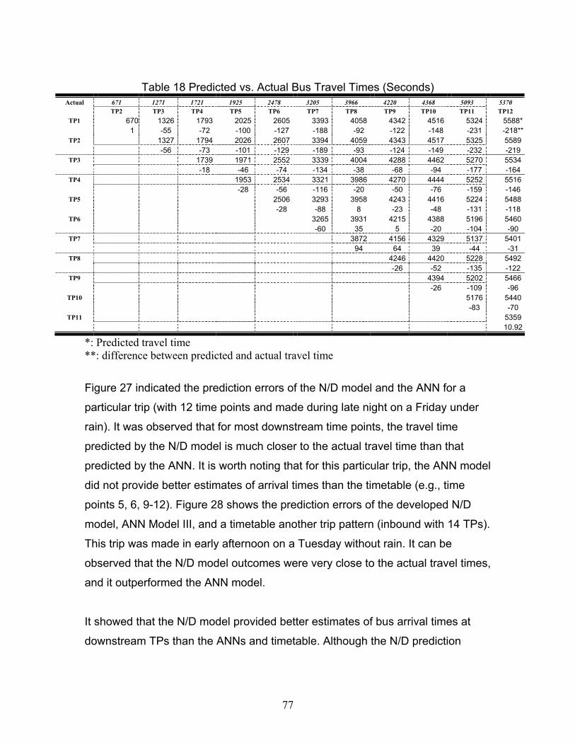
Table 18 Predicted vs. Actual Bus Travel Times (Seconds)
Actual 671 1271 1721 1925 2478 3205 3966 4220 4368 5093 5370 TP2 TP3 TP4 TP5 TP6 TP7 TP8 TP9 TP10 TP11 TP12
TP1 670 1326 1793 2025 2605 3393 4058 4342 4516 5324 5588* 1 -55 -72 -100 -127 -188 -92 -122 -148 -231 -218**
TP2 1327 1794 2026 2607 3394 4059 4343 4517 5325 5589 -56 -73 -101 -129 -189 -93 -124 -149 -232 -219
TP3 1739 1971 2552 3339 4004 4288 4462 5270 5534 -18 -46 -74 -134 -38 -68 -94 -177 -164
TP4 1953 2534 3321 3986 4270 4444 5252 5516 -28 -56 -116 -20 -50 -76 -159 -146
TP5 2506 3293 3958 4243 4416 5224 5488 -28 -88 8 -23 -48 -131 -118
TP6 3265 3931 4215 4388 5196 5460 -60 35 5 -20 -104 -90
TP7 3872 4156 4329 5137 5401 94 64 39 -44 -31
TP8 4246 4420 5228 5492 -26 -52 -135 -122
TP9 4394 5202 5466 -26 -109 -96
TP10 5176 5440 -83 -70
TP11 5359 10.92
*: Predicted travel time **: difference between predicted and actual travel time
Figure 27 indicated the prediction errors of the N/D model and the ANN for a
particular trip (with 12 time points and made during late night on a Friday under
rain). It was observed that for most downstream time points, the travel time
predicted by the N/D model is much closer to the actual travel time than that
predicted by the ANN. It is worth noting that for this particular trip, the ANN model
did not provide better estimates of arrival times than the timetable (e.g., time
points 5, 6, 9-12). Figure 28 shows the prediction errors of the developed N/D
model, ANN Model III, and a timetable another trip pattern (inbound with 14 TPs).
This trip was made in early afternoon on a Tuesday without rain. It can be
observed that the N/D model outcomes were very close to the actual travel times,
and it outperformed the ANN model.
It showed that the N/D model provided better estimates of bus arrival times at
downstream TPs than the ANNs and timetable. Although the N/D prediction
77

might be less accurate for example at TP1 to TP2 (Figure 28), in general, the
prediction errors are less than 5 percent.
0
10
20
30
NJT
MET ROPARK
ST AT ION
INMAN AVE &
WOOD AVE
W INMAN AVE &
ST GEORGES
AVE
MAIN ST & E
MILT ON AVE
SAINT
GEORGES AVE &
WOOD AVE
E JERSEY ST &
BROAD ST
NWK AIRPORT
T ERM A
NWK AIRPORT
T ERM B
NWK AIRPORT
T ERM C
BROAD ST &
EDISON PL
PENN ST AT ION
BUS LANES
Time Points
Trav
el T
ime
Erro
r (%
)
Schedule Error ANN Error N/D Error
Figure 27 Prediction Errors from TP1 to All Time Points (Model I) The deviation between the predicted and actual arrival times, as well as
scheduled and actual arrival times at each time point were shown in Figures 29
through 36. It was observed that for each pattern, the deviation between the
predicted and actual arrival times is smaller than that between the scheduled and
actual arrival times at all time points. The boundary of the arrival time variations
between schedule and actual travel times increases as the index of time points
increases. This might be contributed by the variation of travel times propagated
as the bus proceeded at further downstream stops. However, for the variations
between the predicted and actual arrival times at time points was rather stable
because the N/D model could dynamically predict bus arrival times based on the
most updated information.
In addition to the evaluation of prediction performance of the variations between
scheduled and actual travel time and the variation between predicted and actual
travel times are compared for all the trips (e.g., inbound or outbound with 12 or
78

0
10
20
30
40
50
NJTMETROPARK
STATION
INMAN AVE &WOOD AVE
W INMAN AVE& ST
GEORGESAVE
MAIN ST & EMILTON AVE
SAINTGEORGES
AVE & WOODAVE
E JERSEY ST& BROAD ST
IKEA FEDERALEXPRESS -NEWARKAIRPORT
NWKAIRPORTTERM A
NWKAIRPORTTERM B
NWKAIRPORTTERM C
BROAD ST &EDISON PL
PENNSTATION BUS
LANES
Time Point
Pred
ictio
n Er
ror (
%)
Schedule Error ANN Error N/D Error
Figure 28 Prediction Errors from TP 1 to All Time Points (Model III)
14 time points). The prediction accuracy was evaluated by computing the root
mean squared error (RMSE), which can be obtained from
∑=
−=N
iii yy
NRMSE
1
2)ˆ(1
(14)
where
= the number of test samples N
= actual travel time of sample i iy
= ANN estimated travel time of sample iy i
The RMSEs are calculated for each bus route segment ( i , defined as the segment
between time points i and ). 1+i
79

TP # Description
1 PENN STATION BUS LANES
2 BROAD ST & BRANFORD PL
3 NWK AIRPORT TERM A
4 NWK AIRPORT TERM B
5 NWK AIRPORT TERM C
6 FEDERAL EXPRESS - NEWARK AIRPORT
7 IKEA
8 BROAD ST & W JERSEY ST
9 SAINT GEORGES AVE & WOOD AVE
10 IRVING ST & BROAD ST
11 W INMAN AVE & ST GEORGES AVE
12 INMAN AVE & WOOD AVE
13 NJT METROPARK STATION
14 WOODBRIDGE CENTER MALL
-40
-30
-20
-10
0
10
201 2 3 4 5 6 7 8 9 10 11 12 13 14
Time Point
Arr
ival
Tim
e D
evia
tion
(min
utes
)
Figure 29 Difference between Predicted and Actual Arrival Times (Pattern PAIWM)
TP # Description
1 PENN STATION BUS LANES
2 BROAD ST & BRANFORD PL
3 NWK AIRPORT TERM A
4 NWK AIRPORT TERM B
5 NWK AIRPORT TERM C
6 FEDERAL EXPRESS - NEWARK AIRPORT
7 IKEA
8 BROAD ST & W JERSEY ST
9 SAINT GEORGES AVE & WOOD AVE
10 IRVING ST & BROAD ST
11 W INMAN AVE & ST GEORGES AVE
12 INMAN AVE & WOOD AVE
13 NJT METROPARK STATION
14 WOODBRIDGE CENTER MALL
-40
-30
-20
-10
0
10
201 2 3 4 5 6 7 8 9 10 11 12 13 14
Time Point
Arr
ival
Tim
e D
evia
tion
(min
utes
)
Figure 30 Difference between Scheduled and Actual Arrival Times (Pattern PAIWM)
80

-30
-25
-20
-15
-10
-5
0
5
10
15
201 2 3 4 5 6 7 8 9 10 11 12 13 14
Time Point
Arr
ival
Tim
e D
evia
tion
(min
utes
)
TP # Description
1 WOODBRIDGE CENTER MALL
2 NJT METROPARK STATION
3 INMAN AVE & WOOD AVE
4 W INMAN AVE & ST GEORGES AVE
5 MAIN ST & E MILTON AVE
6 SAINT GEORGES AVE & WOOD AVE
7 E JERSEY ST & BROAD ST
8 IKEA
9 FEDERAL EXPRESS - NEWARK AIRPORT
10 NWK AIRPORT TERM A
11 NWK AIRPORT TERM B
12 NWK AIRPORT TERM C
13 BROAD ST & EDISON PL
14 PENN STATION BUS LANES
Figure 31 Difference between Predicted and Actual Arrival Times (Pattern WMIAP)
TP # Description
1 WOODBRIDGE CENTER MALL
2 NJT METROPARK STATION
3 INMAN AVE & WOOD AVE
4 W INMAN AVE & ST GEORGES AVE
5 MAIN ST & E MILTON AVE
6 SAINT GEORGES AVE & WOOD AVE
7 E JERSEY ST & BROAD ST
8 IKEA
9 FEDERAL EXPRESS - NEWARK AIRPORT
10 NWK AIRPORT TERM A
11 NWK AIRPORT TERM B
12 NWK AIRPORT TERM C
13 BROAD ST & EDISON PL
14 PENN STATION BUS LANES
-30
-25
-20
-15
-10
-5
0
5
10
15
201 2 3 4 5 6 7 8 9 10 11 12 13 14
Time Point
Arr
ival
Tim
e D
evia
tion
(min
utes
)
Figure 32 Difference between Scheduled and Actual Arrival Times (Pattern WMIAP)
81

-40
-30
-20
-10
0
10
201 2 3 4 5 6 7 8 9 10 11 12
Time Point
Arr
ival
Tim
e D
evia
tion
(min
utes
)
TP # Description
1 WOODBRIDGE CENTER MALL
2 NJT METROPARK STATION
3 INMAN AVE & WOOD AVE
4 W INMAN AVE & ST GEORGES AVE
5 MAIN ST & E MILTON AVE
6 SAINT GEORGES AVE & WOOD AVE
7 E JERSEY ST & BROAD ST
8 NWK AIRPORT TERM A
9 NWK AIRPORT TERM B
10 NWK AIRPORT TERM C
11 BROAD ST & EDISON PL
12 PENN STATION BUS LANES
Figure 33 Difference between Predicted and Actual Arrival Times (Pattern WM-AP)
-40
-30
-20
-10
0
10
201 2 3 4 5 6 7 8 9 10 11 12
Time Point
Arr
ival
Tim
e D
evia
tion
(min
utes
)
TP # Description
1 WOODBRIDGE CENTER MALL
2 NJT METROPARK STATION
3 INMAN AVE & WOOD AVE
4 W INMAN AVE & ST GEORGES AVE
5 MAIN ST & E MILTON AVE
6 SAINT GEORGES AVE & WOOD AVE
7 E JERSEY ST & BROAD ST
8 NWK AIRPORT TERM A
9 NWK AIRPORT TERM B
10 NWK AIRPORT TERM C
11 BROAD ST & EDISON PL
12 PENN STATION BUS LANES
Figure 34 Difference between Scheduled and Actual Arrival Times (Pattern WM-AP)
82

TP # Description
1 PENN STATION BUS LANES
2 BROAD ST & BRANFORD PL
3 NWK AIRPORT TERM A
4 NWK AIRPORT TERM B
5 NWK AIRPORT TERM C
6 BROAD ST & W JERSEY ST
7 SAINT GEORGES AVE & WOOD AVE
8 IRVING ST & BROAD ST
9 W INMAN AVE & ST GEORGES AVE
10 INMAN AVE & WOOD AVE
11 NJT METROPARK STATION
12 WOODBRIDGE CENTER MALL
Figure 35 Difference between Predicted and
-30
-25
-20
-15
-10
-5
0
5
10
15
201 2 3 4 5 6 7 8 9 10 11 12
Time Point
Arr
ival
Tim
e D
evia
tion
(min
utes
)
Actual Arrival Times (Pattern PA-WM)
-30
-25
-20
-15
-10
-5
0
5
10
15
201 2 3 4 5 6 7 8 9 10 11 12
Time Point
Arr
ival
Tim
e D
evia
tion
(min
utes
)
TP # Description
1 PENN STATION BUS LANES
2 BROAD ST & BRANFORD PL
3 NWK AIRPORT TERM A
4 NWK AIRPORT TERM B
5 NWK AIRPORT TERM C
6 BROAD ST & W JERSEY ST
7 SAINT GEORGES AVE & WOOD AVE
8 IRVING ST & BROAD ST
9 W INMAN AVE & ST GEORGES AVE
10 INMAN AVE & WOOD AVE
11 NJT METROPARK STATION
12 WOODBRIDGE CENTER MALL
Figure 36 Difference between Scheduled and Actual Arrival Times (Pattern PA-WM)
83

Figures 37 through 40 show the performance comparison of the dynamic
algorithm, the ANN models, and the bus timetable for trips originating from time
point 1 and arriving at each downstream time points, for studied patterns WM-
AP, PA-WM, WMIAP, and PAIWM, respectively.
It can be observed that from all trips statistic analysis, the N/D model, with a
lower RMSE, always performs better than the ANN model. This is as expected
since it has incorporated latest bus arrival information into the prediction. Also,
the ANN generally give better indication of bus travel times than the timetable,
except for outbound trips (pattern 1) arriving at time points 7 through12 from time
point 1. For these particular trips, the maximum difference is less than 60
seconds.
BR
0
100
200
300
400
500
600
700
800
NJT
MET ROPARK
ST AT ION
INMAN AVE &
WOOD AVE
W INMAN AVE &
ST GEORGES
AVE
MAIN ST & E
MILT ON AVE
SAINT
GEORGES AVE
& WOOD AVE
E JERSEY ST &
OAD ST
NWK AIRPORT
T ERM A
NWK AIRPORT
T ERM B
NWK AIRPORT
T ERM C
BROAD ST &
EDISON PL
PENN ST AT ION
BUS LANES
Time Point
Schedule ANN Output N/D Output
Figure 37 Performance Comparison (Pattern WM-AP)
84
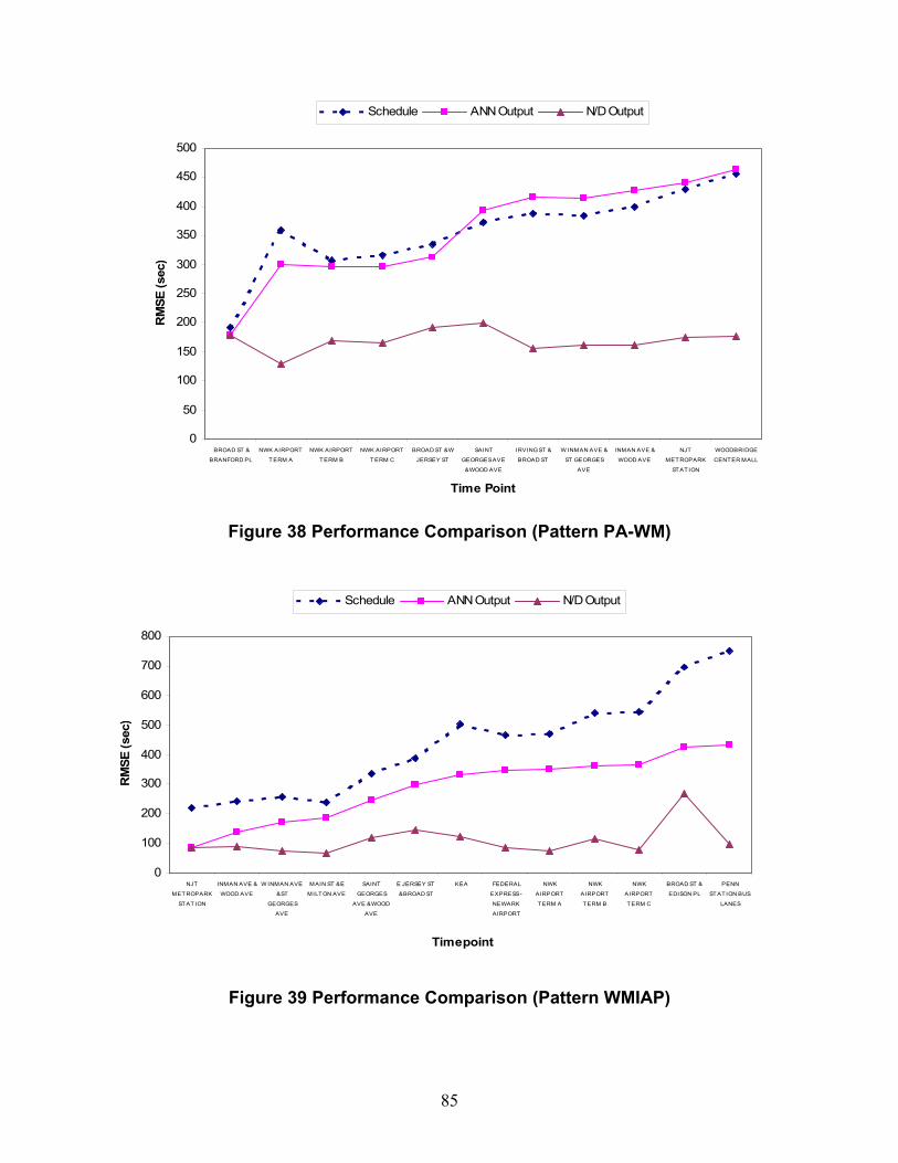
0
50
100
150
200
250
300
350
400
450
500
BROAD ST &
BRANFORD PL
NWK AIRPORT
T ERM A
NWK AIRPORT
T ERM B
NWK AIRPORT
T ERM C
BROAD ST & W
JERSEY ST
SAINT
GEORGES AVE
& WOOD AVE
IRVING ST &
BROAD ST
W INMAN AVE &
ST GEORGES
AVE
INMAN AVE &
WOOD AVE
NJT
MET ROPARK
ST AT ION
WOODBRIDGE
CENT ER MALL
Time Point
RM
SE (s
ec)
Schedule ANN Output N/D Output
Figure 38 Performance Comparison (Pattern PA-WM)
I
0
100
200
300
400
500
600
700
800
NJT
MET ROPARK
ST AT ION
INMAN AVE &
WOOD AVE
W INMAN AVE
& ST
GEORGES
AVE
MAIN ST & E
MILT ON AVE
SAINT
GEORGES
AVE & WOOD
AVE
E JERSEY ST
& BROAD ST
KEA FEDERAL
EXPRESS -
NEWARK
AIRPORT
NWK
AIRPORT
T ERM A
NWK
AIRPORT
T ERM B
NWK
AIRPORT
T ERM C
BROAD ST &
EDISON PL
PENN
ST AT ION BUS
LANES
Timepoint
RM
SE (s
ec)
Schedule ANN Output N/D Output
Figure 39 Performance Comparison (Pattern WMIAP)
85
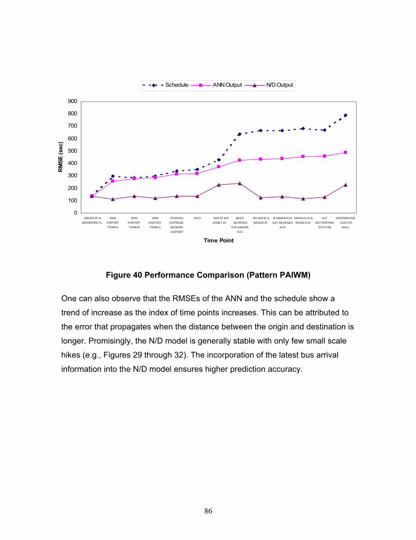
BR
J
0
100
200
300
400
500
600
700
800
900
BROAD ST &
BRANFORD PL
NWK
AIRPORT
T ERM A
NWK
AIRPORT
T ERM B
NWK
AIRPORT
T ERM C
FEDERAL
EXPRESS -
NEWARK
AIRPORT
IKEA OAD ST & W
ERSEY ST
SAINT
GEORGES
AVE & WOOD
AVE
IRVING ST &
BROAD ST
W INMAN AVE
& ST GEORGES
AVE
INMAN AVE &
WOOD AVE
NJT
MET ROPARK
ST AT ION
WOODBRIDGE
CENT ER
MALL
Time Point
RM
SE (s
ec)
Schedule ANN Output N/D Output
Figure 40 Performance Comparison (Pattern PAIWM)
One can also observe that the RMSEs of the ANN and the schedule show a
trend of increase as the index of time points increases. This can be attributed to
the error that propagates when the distance between the origin and destination is
longer. Promisingly, the N/D model is generally stable with only few small scale
hikes (e.g., Figures 29 through 32). The incorporation of the latest bus arrival
information into the N/D model ensures higher prediction accuracy.
86

CHAPTER 8
CONCLUSIONS In this study, the NJ Transit’s APC data were applied in developing bus travel
time prediction models. Though there were some inconsistent data existing in the
APC data, the APC unit has demonstrated its effectiveness to collect detailed
bus operational information (e.g., on/off passenger number, open/close time,
etc). The data and the process procedure discussed in chapter 5, could generate
accurate information for model development, (e.g., weather information, arrival
times at time points, numbers of passengers boarding and alighting at time points
and between them). The process of the APC data could be further developed as
a standard procedure in the future study.
Artificial neural networks (ANN) were developed based on historic bus trip
information for predicting bus arrival times. The developed ANNs have
demonstrated their capability to model complex nonlinear systems, such as a
model for bus travel times. In the developed Neural/Dynamic (N/D) model, the
Kalman filtering algorithm has been integrated with the ANN because of its
dynamic features to adapt to stochastic conditions in real time. Thus the
developed N/D model could provide accurate prediction with data collected by
APC units.
By given trip starting time (time of day), day of week, and weather (precipitation)
condition, the developed ANN is able to generate estimated travel times between
each pair of time points along the trip. The estimated travel time was then used
as input to the developed N/D model to approximate the predicted travel time to a
particular destination (any downstream time points).
After evaluating the developed bus travel time prediction models, it has shown
that the ANN models generally gave a better estimation of travel times than that
posed on the timetable. The N/D model outperformed the ANN models in most
87

time points. The results demonstrated that the N/D model can significantly
improve the error when predicting bus travel times.
It is necessary to note several issues that surfaced during the modeling process.
The primary concern has been the insufficient data in training neural networks.
In this study, the database only contains trips made during Year 2002. The
amount of usable data is quite limited. Even though measures were taken to
reduce the number of network weights in the ANN models, the recommended
data amount to network weights ratio was still insufficient in certain cases. It is
desirable to have more data to train and test the ANN models.
Another major concern has been the data quality. During pre-processing, it was
found that large discrepancies exist in Year 2002 data. Such problems include
inconsistent distance traveled between time points, inaccurate time point
locations, incomplete trip records, etc. Corrections had to be made manually and
some trip data had to be abandoned for model development purpose, which
certainly contributed to the limited data size in the ANN modeling process.
With the increase in the amount of available data, we believe that the
methodology developed in this study will become a powerful tool for bus arrival
time prediction. Future study may explore the inclusion of other variables such
as passenger counts, dwell times into the ANN model (they were not included
because of the limited training samples).
88

REFERENCES 1. Federal Transit Administration (2000) Advanced Public Transportation
Systems: The State of the Art, Update 2000. http://www.itsdocs.fhwa.dot.gov/jpodocs/repts_te/13583.pdf
2. Federal Highway Administration (2000) Automatic Vehicle Location
Successful Transit Applications: A Cross-Cutting Study. FHWA- OP-99-022/FTA-TRI-11-99-12. http://www.itsdocs.fhwa.dot.gov/jpodocs/repts_te/8v301!.pdf
3. Boldt, R. (1998) Automatic Fleet Control: State of the Practice. Urban
Transport International, London, UK. No.18, pp. 24-27. 4. Casey, R. (2000) Chapter 5: What Have We Learned About Advanced Public
Transportation Systems? What Have We Learned About Intelligent Transportation Systems? John A. Volpe National Transportation Systems Center. http://www.itsdocs.fhwa.dot.gov//JPODOCS/REPTS_TE/@@101!.PDF
5. Peng, Z-R; Beimborn, E, Octania, S, Zygowicz, R. (1999) Evaluation of the
Benefits of Automated Vehicle Location Systems for Small and Medium Sized Transit Agencies. Transportation Research Board, SPR-0092-45-84. http://www.uwm.edu/Dept/CUTS/00365.pdf
6. Okunieff, P. (1997) AVL Systems for Bus Transit. Transportation Cooperative
Research Program (TCRP) Synthesis 24. http://www.tcrponline.org/PDF/TSYN24.pdf
7. Sterns, M., Sussman, D., and Belcher, J. (1999) Denver RTDS Computer
Aided Dispatch-Automatic Vehicle Location Systems – the Human Factors Consequences. DOT-VNTSC-FTA-98-8/DOT-FTA-TRI-11-99-29. http://www.itsdocs.fhwa.dot.gov//JPODOCS/REPTS_TE/8R301!.PDF
8. Weatherford, M. (2000) Assessment of the Denver Regional Transportation
District's Automatic Vehicle Location System. DOT-VNTSC-FTA-00-04/FTA-MA-26-7007-2000-2.
9. http://www.nextbus.com/predictor/newUserWelcome.shtml, 02/15/2003. 10. http://www.nextbus.com/predictor/simpleRouteSelector.shtml?a=ART,
02/15/2003. 11. http://www.actransit.org/, 02/15/2003. 12. http://www.ci.fairfax.va.us/Services/CueBus/NextBus.htm, 02/15/2003.
89
13. http://www.ci.vail.co.us, 02/15/2003.
14. http://www.sfmuni.com, 02/15/2003.
15. http://www.tri-met.org/its.pdf, 02/15/2003.
16. http://www.aata.org/aos.asp, 02/15/2003. 17. http://www.its.washington.edu/transitwatch/, 02/15/2003. 18. Dailey, D., and Maclean, S. (2001) MyBus: Helping Bus Riders Make
Informed Decisions. IEEE Intelligent Systems. Vol.16, No. 1, 84-87. 19. http://www.fta.dot.gov/brt/guide/info.html, 02/15/2003. 20. http://www.fta.dot.gov/brt/projects/albany.html, 02/15/2003. 21. Rossetti, M. D. (1998) Field Testing and Evaluation of the Transit Integrated
Monitoring System. Transit Cooperative Research Program – IDEA. Transportation Research Board.
22. Dailey, D., Maclean, S., Cathey, F., and Wall, Z., (2001) Transit Vehicle
Arrival Prediction: Algorithm And Large-Scale Implementation, Journal of the Transportation Research Board, 1771, 46-51.
23. Lin, W., and Zeng, J., (1999) An Experimental Study On Real Time Bus
Arrival Time Prediction With GPS Data, Transportation Research Record, 1666, 101-109.
24. http://translink.tamu.edu/docs/Research/BusArrivalPrediction/PredictionAlgorit
hms.cfm, 02/15/2003. 25. Chien, S., Ding, Y., and Wei, C., (2002) Dynamic Bus Arrival Time Prediction
With Artificial Neural Networks, Journal of Transportation Engineering, ASCE, Vol. 128, No. 5, pp 429~438.
26. Multisystems, White Paper on Literature Review of Real-time Transit
Information Systems, FTA Real-Time Transit Information Assessment, (2002).
27. Peng, Z. R., and Jan, O., (1999) “Assessing Means of Transit Information
Delivery for Advanced Public Transportation Systems,” Transportation Research Board, #1666, pp. 92-100, Washington, D.C.
90
28. Dailey, D. J., Fisher, G., and Maclean, S.,(1999) “BusView and Transit Watch: An Update on Two Products from the Seattle SMART TREK Model Deployment Initiative,” 6th World Congress on ITS, Toronto.
29. Maclean, S., and Dailey, D., “Real-time Bus Information on Mobile Devices,”
www.its.washington.edu/its_pubs.html. 30. Maclean, S. D. and Dailey, D., “The Use of Wireless Internet Service to
Access Real-time Transit Information, Wireless Internet access to Real-time Transit Information,” www.its.washington.edu/its_pubs.html.
31. Casey, R., et al, Advanced Public Transportation Systems: The State of the
Art Update 2000, FTA, Washington, D.C. 2000. 32. Hua, J., and Faghri, A., (1994) Application of ANNs to IVHS. Transportation
Research Record, 1453, pp83-90.
33. Chin, S, Hwang, H., and Pei, T., (1994) Using Neural Networks to Synthesize Origin-Destination Flows in a Traffic Circle. Transportation Research Record, 1457, pp134-142.
34. Dougherty, M., (1995) A Review of Neural Networks Applied to Transport. Transportation Research, Vol.3C, No.4, pp247-260.
35. Kalaputapu R., and Demetsky, M., (1995) Modeling Schedule Deviation of Busses Using Automatic Vehicle-Location Data and Artificial Neural Networks. Transportation Research Record, 1497, pp44-52.
36. Smith, B. L., and Demetsky, M. J., (1995) Short-term Traffic Flow Prediction: Neural Network Approach. Transportation Research Record, 1453, pp98-104.
37. Zhang, H., Ritchie, S., and Lo, Z., (1997) Macroscopic Modeling of Freeway Traffic Using an Artificial Neural Network. Transportation Research Record, 1588, pp110-119.
38. Chang, G., and Su, C. (1995) Predicting Intersection Queue with Neural Network Models. Transportation Research, Vol.3C, No.3, pp175-191.
39. Wei, C., and Yang, Y., (1998) Assessing Input Layer Elements of Artificial Neural Networks – An Empirical Study for Transit Containers Forecast in Kaohsiung Port. Submitted to Journal of the Chinese Institute of Transportation.
40. Ding, Y., and Chien, S., (2000) The Prediction of Bus Arrival Times with Link-
based Artificial Neural Networks, International Conference on Computational
91

92
Intelligence & Neurosciences (CI&N) – Intelligent Transportation Systems, Conference Proceedings, pp. 730-733, Atlantic City, New Jersey.
41. McFadden J., Yang W.T., and Durrans, S. R., (2001) Application of Artificial
Neural Networks to Predict Speeds on Two-Lane Rural Highways. Transportation Research Record, 1751, pp9-17.
42. http://www.mathworks.com/access/helpdesk/help/toolbox/nnet/nnet.shtml,
02/15/2003.