use of electrical resistivity methods for study of some faults in the jharia coalfield, india

Geoexploration 18 (1980) 201-220 o Elsevier Scientific Publishing Company, Amsterdam - Printed in The Netherlands

USE OF ELECTRICAL RESISTIVITY METHODS FOR STUDY OF SOME FAULTS IN THE JHARIA COALFIELD, INDIA

R.K. VERMA, N.C. BHUIN and C.V. RAO

Indian School of Mines, Dhanbad (India)

(Received February 9, 1979; accepted October 16, 1979)

ABSTRACT

Verma, R.K., Bhuin, N.C. and Rao, C.V., 1980. Use of electrical resistivity methods for study of some faults in the Jharia coalfield, India. Geoexploration, 18: 201-220.

Two prominent faults, Dumra fault and the Southern Boundary fault, belonging to the Jharia coalfield, India, have been studied using electrical resistivity methods. A few normal configurations have been used to study the Dumra fault, whereas the Southern Bound- ary fault has been studied using the horizontal profiles and vertical soundings azimuthally as discussed by Al-Chalabi (1969) and Kumar (1973).

The results over the Dumra fault suggest the two-electrode configuration to be the most suitable one for mapping this type of discontinuity as far as the shape and amplitudes of the anomaly are concerned. Other configurations show appreciable noise due to the near surface inhomogeneities.

The results over the Southern Boundary fault prove the usefulness of the Al-Chalabi profiles in study of this type of discontinuity in the field. The half-Schlumberger profiles give good indication of the fault. The two-electrode profiles and soundings do not give useful indication of the fault due to small resistivity contrast between the formations on its either side. The peaks and the troughs for all the profiles over the fault are seen to be- come less prominent, as the angle between the profile lines and the fault decreases from 90” to 30”.

A quartz dyke lying very close to the fault and having a width of about 100 m is seen to be well reflected through all the azimuthal profiles and soundings.

INTRODUCTION

Different techniques (normal as well as azimuthal profilings and soundings) using electrical resistivity method have been suggested for the study of faults/ contacts by several workers, viz., Tagg (1930), Logn (1954), Kunetz (1966), Van Nostrand and Cook (1966), Al-Chalabi (1969), Zohdy (1970), Kumar (1973) and Telford et al. (1976). The results of the theoretical studies clearly suggest the successful application for delineating the above mentioned struc- tures using most of the techniques. However, actual field cases reported are very few and the nature of resistivity anomalies obtained across discontinuities in the field is known only for a few electrode configurations. The usefulness

of various configurations for study of such problems in the field has yet to be established.

Keeping this in view, a few normal configurations like Wenner, two- electrode and half-Schlumberger have been used to study a prominent fault, known as the Dumra fault, belonging to the Jharia coalfield, an important coalfield in India, situated between 23” 37’-23” 52’N and 86”06’-86”30’E in the Dhanbad district of Bihar. Another prominent boundary fault known as the Southern Boundary fault of the same coalfield has also been studied, using azimuthally the four longitudinal spreads of Al-Chalabi (1969), two- electrode configurations as studied by Kumar (1973) as well as half-schlumberger configurations. The results obtained are discussed in this paper.

SURVEY AREAS AND LOCATION OF THE PROFILES

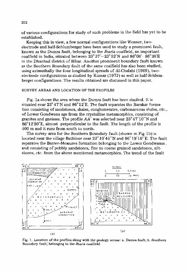
Fig. la shows the area where the Dumra fault has been studied. It is situated near 23”47’N and 86”12’E. The fault separates the Barakar formation consisting of sandstones, shales, conglomerates, carbonaceous shales, etc., of Lower Gondwana age from the crystalline metamorphics, consisting of granites and gneisses. The profile AA’ was selected near 23”47’10”N and 86”12’20”E, almost perpendicular to the fault. The length of the profile is 400 m and it runs from south to north.

The survey area for the Southern Boundary fault (shown in Fig. lb) is located near the village Batbinor near 23” 10’45”N and 86” 19’10”E. The fault separates the Barren-Measures formation belonging to the Lower Gondwanas , and consisting of pebbly sandstones, fine to coarse grained sandstones, silt- stones, etc. from the above mentioned metamorphics. The trend of the fault

- _

(b)

Fig. 1. Location of the profiles along with the geology across: a. Dumra fault; b. Southern Boundary fault,. belonging to the Jharia coalfield.

203

is NW-SE and the traverses were taken approximately at angles 0 = 90”, 60”, 45”, 30” and 15” to the strike of the fault. An exposure of a quartz dyke is seen to be present very close to the site on the south side of the fault. The dyke is at an angle to the strike of the fault. Both the areas are free from all types of disturbances and have nearly smooth surface topography.

FIELD OBSERVATIONS

All the field observations were carried out using an ‘Aquameter’ fabricated by Sparkonix, Poona, India. Steel electrodes were used for sending a current into the ground and measurements of potential. The instrument produces square wave a.c. at 4 Hz.

The configurations used in horizontal profiles across the Dumra fault area: Wenner with L = 60 and 150 m (L is the total electrode separation); two- electrode with L = 20 and 50 m; and half-Schlumberger with L = 25 and 60 m along one profile (AA’) only. The Schlumberger configurations were used to take vertical electrical soundings on either side of the fault and to construct a geoelectric section.

The azimuthal horizontal resistivity profiles were carried out along A 1 A; , A2 A;, A4Ak at different angles to the strike of the Southern Boundary fault as shown in Fig.lb. The total electrode separation (L) was kept at 300 m for t (potential electrode separations) = 5, 25, 100 and 200 m and at 30 m for t = 1, 5,lO and 20 m for Al-Chalabi profiles, L = 10, 20, 40 and 150 m for half-Schlumberger profiles and L = 5, 20, 50 and 100 m for two-electrode profiles. The length of all these profiles was kept at 250 m except for the half-Schlumberger profiles along A4 AI, , whose length was 280 m for delineating the width of the quartz dyke. The vertical electrical soundings were taken using Schlumberger configuration along all the three profiles to get the geoelectric sections. The azimuthal two-electrode soundings were taken along the above mentioned profiles and also along A3 A;, A, A; at 0 = 45” and 15”) respectively.

It may be mentioned here that the total electrode separations (L) for all the above mentioned horizontal profiles were chosen on the basis of the sounding results, keeping in view the depth of investigation characteristics as given by Roy and Apparao (1971).

RESULTS OF STUDIES ACROSS THE DUMRA FAULT

Vertical electrical soundings

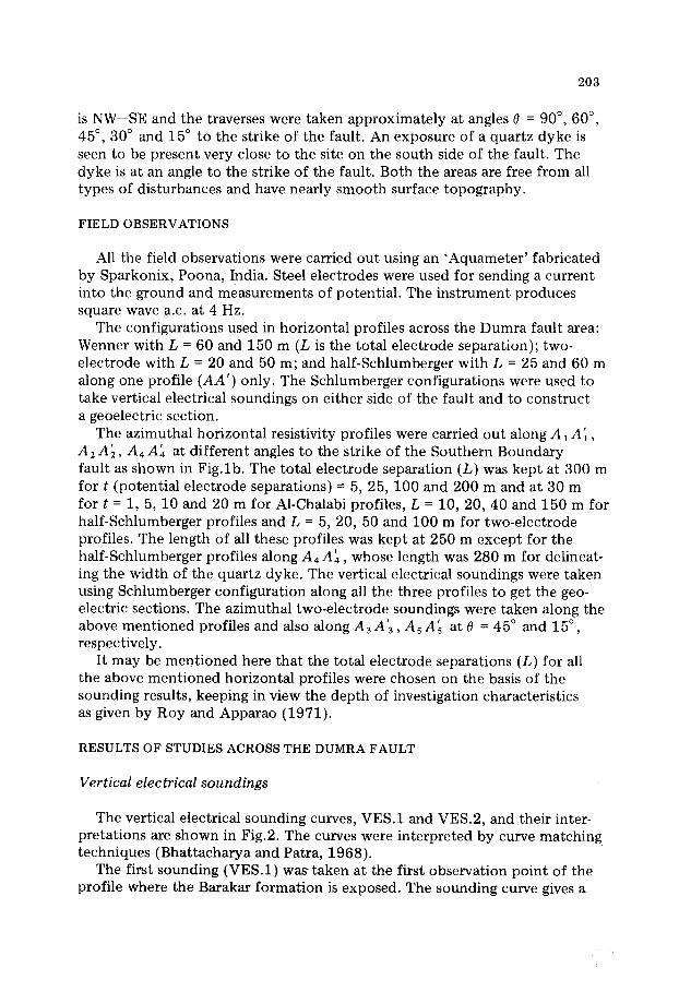
The vertical electrical sounding curves, VES.l and VES.2, and their inter- pretations are shown in Fig.2. The curves were interpreted by curve matching techniques (Bhattacharya and Patra, 1968).

The first sounding (VES.l) was taken at the first observation point of the profile where the Barakar formation is exposed. The sounding curve gives a

VES.1 VES. 2

p, = 600 IL m , h, = 1.5 I ~=76Am,h,=ZOm

p2= zoonm, h,= - ~2=664fim, h,= O.Z.

Fig. 2. Results of Schlumberger soundings, VES.1 and VES.2, along the profile AA' across the Dumra fault (see Fig.1). The results of VES.l indicate that the top 1.5 m of the Barakar formation is highly resistive having a resistivity value of about 600 n m.

descending type two-layer appearance. The resistivity of the first layer of the exposed Barakar formation is about 600 L? m upto a depth of 1.5 m from the surface, below which the resistivity is about 200 n m.

The second sounding (VES.2) was taken at a distance R = 360 m (R is the distance from the origin of the profile) over the metamorphics. The nature of this sounding curve is just opposite to that of VES.l, i.e., ascending type giving two-layer appearance. The interpreted results suggest the presence of a weathered layer (with resistivity of 76 s2 m) within the metamorphics upto a depth of about 20 m below the surface.

The results of the above two vertical electrical sounding curves indicate the presence of resistivity contrast between the Barakar formation and the metamorphics at shallow as well as at greater depths.

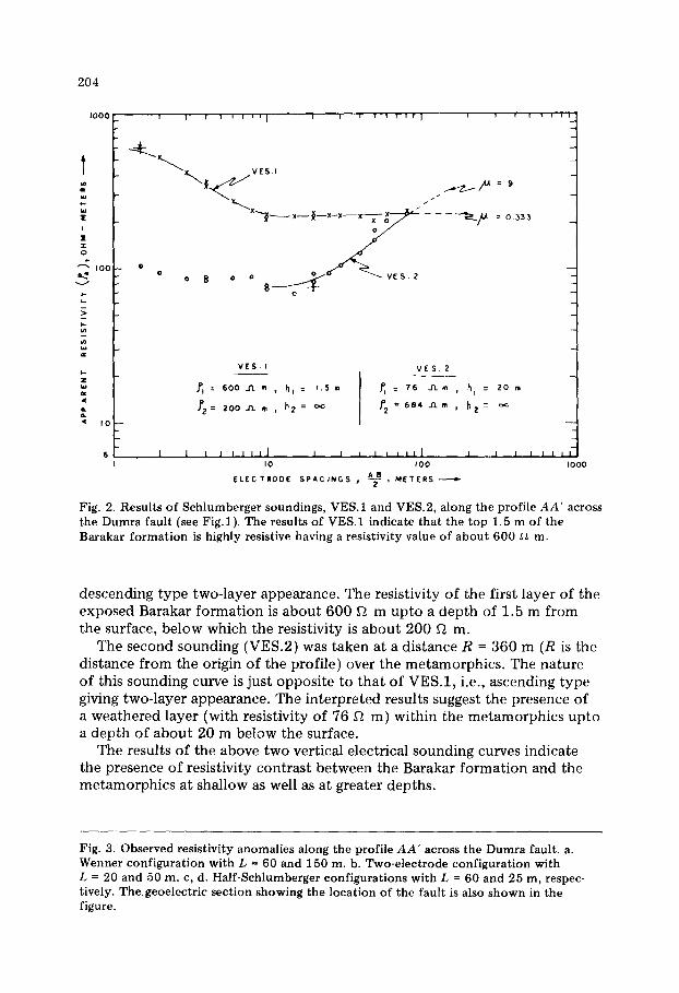
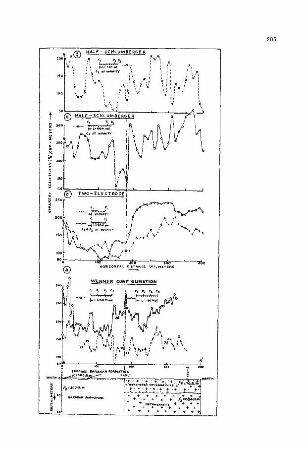
Fig. 3. Observed resistivity anomalies along the profile AA' across the Dumra fault. a. Wenner configuration with L = 60 and 150 m. b. Two-electrode configuration with L = 20 and 50 m. c, d. Half-Schlumberger configurations with L = 60 and 25 m, respectively. The geoelectric section showing the location of the fault is also shown in the figure.

HALF - SCHLUHBERGE R

WENNER CONFIGURATION

206

Horizontal resistivity profiles

The apparent resistivity anomalies obtained through Wenner, two-electrode and half-Schlumberger configurations are shown in Fig.3 along with the geoelectric section (drawn on the basis of the results obtained through soundings as well as profilings) across the fault.

Wenner profiles

The Wenner profiles using L = 60 and 150 m (Fig.3a) show irregular variations of apparent resistivity values over the Barakar formation as well as over the metamorphics. Both the profiles show high values of apparent resistivity at the beginning of the profile due to the presence of the exposed dry Barakar formation. The average value of apparent resistivity is found to be nearly the same on either side of the fault for L = 60 m, whereas for L = 150 m, an increase in apparent resistivity value can be seen over the metamorphics due to the larger depth of investigation. Although two peaks, having values of about 170 S2m for L = 60 m, and 280 SIrn for L = 150 m, are found at a distance R = 180 m, just over the fault, it is difficult to ascribe these peaks to the fault only in view of the large fluctuations present along the profile.

Two-electrode profiles

The apparent resistivity anomalies obtained through these configurations using L = 20 and 50 m show (Fig.3b) rather smooth variation along the profile. The fault can be fairly accurately located at a distance R = 180 m seeing the sharp change in apparent resistivity values on both the curves. The change in apparent resistivity values over the fault range from 110 to 160 L? m for L = 20 m and from 130 to 240 Q m for L = 50 m profiles. Both the profiles show more or less the same apparent resistivity values over the Barakar formation but a difference can be noted over the metamorphics on account of larger depth of investigation for L = 50 m profile.

Half-Schlumberger profiles

The half-Schlumberger profiles (Fig.3qd) for L = 25 and 60 m also show irregular variations of apparent resistivity as obtained through Wenner profiles (discussed earlier) but the peaks over the fault are more prominent here particularly for L = 60 m. The sharp peaks suggest that the fault is nearly vertical. The change in resistivity values over the fault range from 140 to 300 fi m for L = 60 m and 90 to 170 C? m for L = 25 m. The other characteristics of these anomalies are the same as discussed earlier for Wenner profiles.

RESULTS AND INTERPRETATION ACROSS THE SOUTHERN BOUNDARY FAULT

The results obtained using Schlumberger soundings and azimuthal profilings along different profiles are discussed below. The sounding curves were interpreted using partial as well as full curve matching techniques (Keller and Frischknecht, 1966; Bhattacharya and Patra, 1968).

Results alongprofile A,A’, (0 = 90”)

Four S~hlumberger soundings (VES.l, VES.2, VES.3 and VES.4), two on either side of the fault, were taken along the profile A 1 A; (location shown in Fig.lb). All the sounding curves show three-layered, A-type appearance and are shown in Fig.4.

VEX1 and VES.2. These two soundings were taken at R = 25 and 95 m over the Barren-Measures on the northern side of the fault. The results of these two soundings are shown in Fig.4a. The interpreted results of both the soundings show an increase in resistivity value with depth within the Barren-Measures formation. The thickness of the first layer of the weathered Barren-Measures is the same (about 3.0 m) at these two locations but the resistivity values are different, about 74 G m at R = 25 m and 37 52 m at R = 95 m. The resistivity of the second layer (partly weathered Barren- Measures) is the same (about 111 8 m) for both the locations, but the thickness varies from 36 to 22.5 m. The third layer, i.e., the hard and compact Barren-Measures show high values of resistivity, of the order of 800-900 52 m.

VES.3 and VES.4. The soundings VES.3 and VES.4 were taken at distances R = 165 and 225 m respectively over the metamorphics on the south side of the fault. The interpretation of these curves (Fig.4b) indicates that the first as well as second iayers within the metamorphics have nearly the same values of resistivity (15 and 75 52 m respectively). The resistivity of the unweathered metamorphics is of the order of 4350-5450 L? m.

The above mentioned results suggest the presence of high resistivity values along the Barren-Measures side as compared to the metamorphics side upto a depth of about 20 m below the surface. At greater depths the resistivity value is appreciably higher underneath the metamorphics than underneath the Barren-Measures.

Horizontal profiles The apparent resistivity curves obtained for profiles using different con-

figurations are shown in Figs.5 and 7 along with the geoelectric section, drawn on the basis of the results obtained through soundings as well as profilings. The theoretical apparent resistivity anomalies across the discontinuity using four longitudinal spreads of different electrode separations after Al- Chalabi (1969) are shown in Fig.6:

\ow

t .

, .“

‘“,

, I

I .“

“S,

-3

209

Al-Chalabi profiles. The profiles were taken using different values of L and t as shown in the figure. The variations of apparent resistivity values on either side of the fault are more or less the same for t = 25, 100 and 200 m profiles (Fig.5a). The nature of these resistivity curves does not give a clear indication of the presence of the fault. The profile for t = 5 m shows one prominent peak (2), another small peak (4) and two clear troughs (1,3). The fault can be located fairly well (near R = 115 m) at the middle point of peak (2) and trough (3) as suggested by Al-Chalabi on a theoretical basis (Fig.Ga). The average values of apparent resistivity are seen to decrease with the increase of the potential electrode separation (t). An increase in resistivity values near R = 185 m over the metamorphics on the profiles using t = 5 and 25 m can be attributed to the presence of the quartz dyke.

The peaks (2,4) and the troughs (1,3) close to the fault are more prominent on the profiles using L = 30 m and t = 1, 5, 10 m as seen in Fig.5b. The fault can be clearly located using Al-Chalabi’s criterion (in between peak (2) and trough (3)). The response of the quartz dyke has not been obtained through these profiles apparently due to their smaller depth of investigation as compared to the profiles discussed earlier.

Half-Schlumberger profiles. The half-Schlumberger profiles (Fig.7a) using L = 10, 20 and 40 m show clear indication of the fault giving rise to the peaks and troughs near the fault zone. The peaks and the troughs for the L = 150 m

profile are not so clear but a sharp change of anomaly is observed at a distance R = 120 m. The quartz dyke does not give any significant response for these profiles.

Two-electrode profiles. The two-electrode profiles (Fig.7b) for L = 100, 50 and 20 m do not show any indication of the presence of the fault but the quartz dyke is clearly reflected for L = 100 m profile. The left edge of the dyke can be marked fairly well at a distance R = 185 m.

Results along profile A, A; (8 = 60” )

Schlum berger soundings Two soundings, VES.5 and VES.6, were taken along the profile A, A; at

two different points on either side of the fault. The sounding curves show three-layered A-type appearance and are shown in Fig.4c. The interpretation is similar to that discussed earlier for VES.l to VES.4. Based on these results, a geoelectric section was constructed as shown in Fig.8.

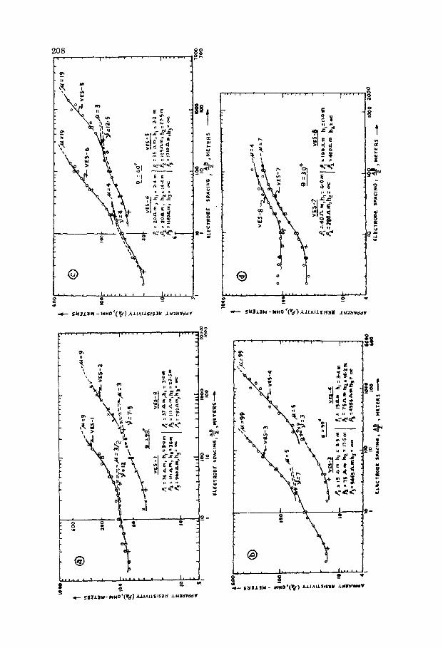
Fig. 4. Results of Schlumberger soundings. a. VES.1, VES.2. b. VES.3, VES.4 along profile A,A’, at 0 = 90”. c. VES.5 and VES.6 along profile A,A; at B = 60”. d. VES.7 and VES.8 along profile A,Al at e = 30” across the Southern Boundary fault.

210 _:’ $3 fbt = _!_

L so

@ __,._Cu_u ; E _?_

30

AL- CHALA81 PROFILES Cl r: Ft cz t

e -90” -_+.__’ ’ ’ ’ IZ5r

2

- = Y$ (WINNER) L

L .z CURRENT ELECTRODE SEPARATION

t t = POTENTIAL ELECTRODE SEPARATION

* I: u * Is- w 2 I I

i “6 I 8 1 Is I I

50 100 IlO I00 zm

:: _ beor

HORIZONTAL DISTANCE CR), METERS -

t s -_;-. L 300

t 25 -i = 500

t - = +!$ WENNER L

t z t = POTENTIAL ELECTRODE SEPARATION w

I Q <

L L 1 I a:

“e I* I , ,

l(M IS0 Ire 10

WORIZONTAL DISTANCE (R), METERS 4 u I *

LOCATION OF VERTICAL ELECTRICAL SOUNDING

;,I, h f, TRUE RESISTIVbTY OF THE FIRST, SECOND AND THIRD LAYER

Fig. 5. Observed resistivity anomalies along the profile AL A', (0 = 90" ) across the Southern Boundary fault. a. Al-Chalabi configurations with L = 300 m and t = 5, 25, 100 and 200 m. b. Al-Chalabi configurations with L = 30 m and t = 1, 5,10 and 20 m. The geoelectric section showing the position of the fault and the quartz dyke is also shown in the figure. 1 = top weathered layer, Barren-Measures; 2 = partly weathered layer, Barren-Measures; 3 = Barren-Measures, unweathered; 4 = top weathered layer, metamorphics; 5 = partly weathered layer, metamorphics; 6 = metamorphics, unweathered; 7 = quartz dyke.

211

4’o (a) 8 = 90°

t I _._.___ - ¶z -

3.0 ~ L 30 t 5 P -r- L 30 _____ _ f-

WENNER 2 -0

. . “_....

l /6 2/6 o 96 6/6 8/6 ‘Of6

DISCONTINURTY

2/6 I I , , t 1 ‘/6 t o 96 , 1 8/6 f ,

P;

‘O/6 1

p2 DlSCONTlNUlT Y

r

P, DlSCONTINUITY A

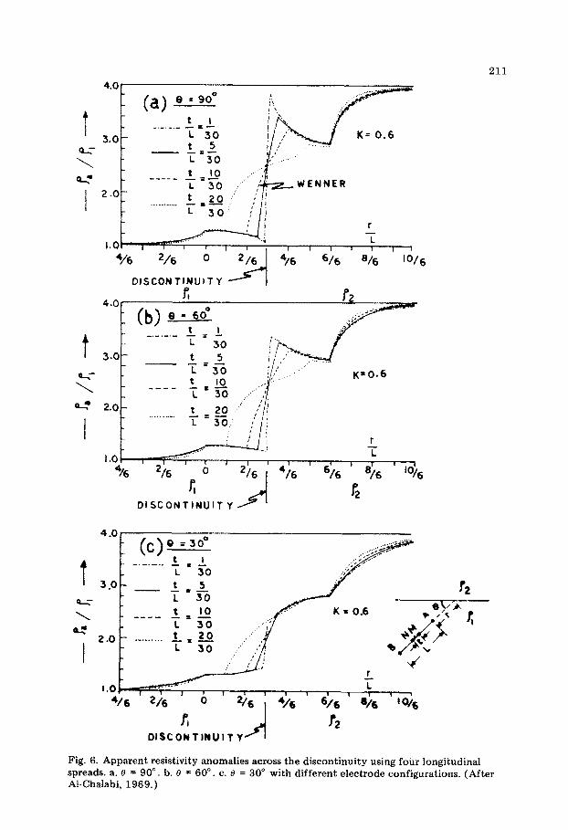
Fig. 6. Apparent resistivity anomalies across the discontinuity using four longitudinal spreads. a. 0 = 90”. b. 0 = 60”. c. e = 30” with different electrode configurations. (After Al-Chalabi, 1969.)

212

300 I--

C, L-.._J L = loom

TWO-ELECTRODE PROFILES

250 -_x_- cL--’ L = 50m

SO- ! I

1 I

O- I 1 1 111 I ,I I 1 J 0 50 100 I50 200 260

HORIZONTAL DISTANCE h),METERS +

c, ?P,

@ -.*.- -

L = iom

HALF - SCHLIJMBERCER

+ + +

INDEX

ml m2 mn]3 m4 i:+::iis 1+‘+16 m7

. LOCATION OF VERTICAL ELECTRICAL SOUNDlN6

J,p,& 4 TRUE RESISTIVITY OF THE FIRST, SECOND &THIRD LAYER

213

Horizontal profiles The apparent resistivity curves obtained through all the configurations

used along the profile Ai A; at 0 = 60” are shown in Fig.8 along with the geoelectric section.

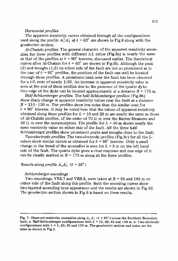
&C/&&i profiles. The general character of the apparent resistivity anomalies for these profiles with different t/L ratios (Fig8a) is nearly the same as that of the profiles at B = 90” traverse, discussed earlier. The theoretical curves after Al-Chalabi for 0 = 60” are shown in Fig.Gb. Although the peak (2) and troughs (1,3) on either side of the fault are not so prominent as in the case of 0 ‘= 90” profiles, the position of the fault can well be located through these profiles. A prominent peak near the fault has been observed for a t/L ratio of nearly l/30. An increase in apparent resistivity value is seen at the end of these profiles due to the presence of the quartz dyke. One edge of the dyke can be located approximately at a distance R = 175 m.

Half-Schlumberger profiles. The half-Schlumberger profiles (Fig.8b) show sharp change in apparent resistivity values near the fault at a distance R = 110-130 m. The profiles show less noise than the similar ones for 0 = 90” traverse. It may be noted here that the values of apparent resistivity obtained along these profiles for L = 10 and 20 m are nearly the same as those of Al-Chalabi profiles, of the order of 70 a m over the Barren-Measures and 40 Q m over the metamorphics. The profile for L = 40 m shows nearly the same resistivity value on either side of the fault. All the three half- Schlumberger profiles show prominent peaks and troughs close to the fault.

Two-electrode profiles. The two-electrode profiles (Fig.&) for all the L- values show similar nature as obtained for 0 = 90” traverse. Only a small change in the trend of the anomalies is seen for L = 5 m on the left hand side of the fault. The quartz dyke gives a clear response and one edge of it can be clearly marked at R = 175 m along all the three profiles.

Results along profile A,Ab (0 = 30”)

Schlumberger soundings Two soundings, VES.7 and VES.8, were taken at R = 55 and 185 m on

either side of the fault along this profile. Both the sounding curves show two-layered ascending type appearance and the results are shown in Fig.4d. The geoelectric section shown in Fig.9 is based on these results.

Fig. 7. Observed resistivity anomalies along A, A; (0 = 90" ) across the Southern Boundary fault. a. Half-Schlumberger configurations with L = 10, 20, 40 and 150 m. b. Two-electrode configurations with L = 5, 20, 50 and 100 m. The geoelectric section and index are the same as shown in Fig. 5.

214 0

N

Cl __+LL= 50m

,,‘[ _++._‘ll L = 20m

TWO- ELECTROOE PROFILES

8 -60’

2eb t-+-t

Cl 91 L = 5m ,x- x _ ~_X_.x-I--*-X

IJO C2 6 Pa AT INFINITY

100

t 50

cn I 0

l

PC , I I I

0 50 100 IS0 100 250

? HORIZONTAL DISTANCE (R),~IETERs - w x Cl 95

- cfipz_

-.-D_.- L= Iom

LL 20m @ _ 220- CGP* /X

t_=40m: HALF - SCHLUMBERGER PROFILES

200 - _ _y__ 8 5 60’

I I 06 1 I ,

0 so 100 150 200 250

HORIZOf$TAL DISTANCE (R), kttERS -

Cl4p,C2f ,

-- Cl PI 5 c2 t

_I_0 T: = z -‘~~‘;,,,,_,ER) ‘i: - 30 AL- CHALABI PRoClLES

yjpz$zt fj --x-m -f-

L 30 -

I5or L-CURRENT ELECTRODE SEP. _ f

/

Oh i _ I

I I I * # 0 10 IO0 150 200 250

700

8

E 0 5 700 w

mlmZm3m41:+:+;15L+*lGm7

. LOCATION OF VERTICAL ELECTRICAL SOUNDING

4 ,& & 4 TRUE RESISTIVITY OF THE FIRST,SfCOND 8 THIRD LAYER

215

Horizontal profiles The resistivity anomalies for the configurations used along this traverse

are shown in Fig.9 along with the geoelectric section. Al-Chalabi profiles. The profiles (Fig.Sa) for all values of t show nearly

the same apparent resistivity values on either side of the fault. The average value of apparent resistivity may be taken as close to 60 L? m upto a distance of R = 165 m, after which an increase is seen on the west side due to the presence of the quartz dyke. All the peaks and the troughs over the fault region are less prominent along these profiles as also shown by Al-Chalabi (Fig.Gc) on a theoretical basis. The general character of the anomalies is quite different from that observed for profile A, A; with 0 = 90”.

Half-SchEumberger profiles. These profiles (Fig.Sb) show a considerable fluctuation as compared to similar ones for 0 = 60”. Although the peak (2) and troughs (1,3) are associated with the fault, another prominent peak is observed on the west side which is associated with the quartz dyke. As al- ready mentioned, the length of these profiles was increased by 30 m to locate the width of the dyke, which is clearly picked up from R = 165- 265 m.

Two-electrode profiles. The two-electrode profiles (Fig.Sc) using L = 5 and 20 m show a small change of resistivity values close to the faulted region. The profile using L = 50 m gives no indication at all. The quartz dyke has been picked up very clearly through all these profiles indicating the presence of one of its edges near R = 165 m.

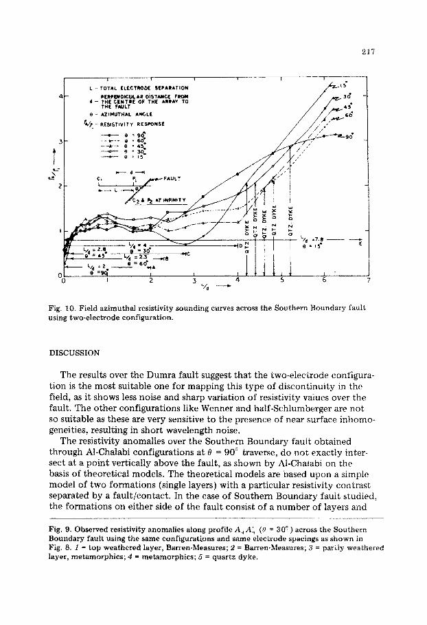
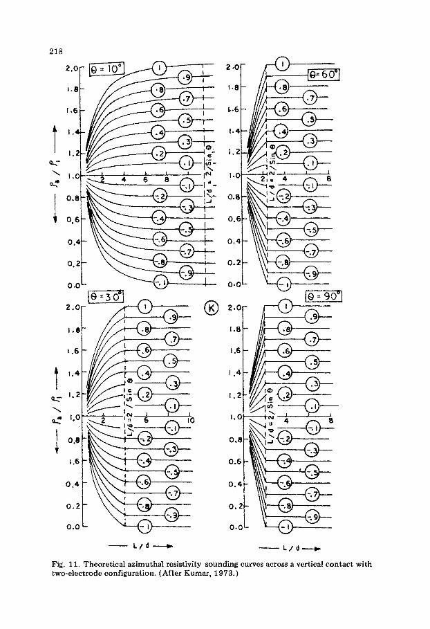
Two-electrode azimuthal soundings. The results of two-electrode azimuthal sounding curves for 0 = 90”, 60”, 45”, 30” and 15” are shown in Fig.10. These are plotted keeping pa/p 1 along the y-axis and L/d along the x-axis (L is the total electrode separation and d is the perpendicular distance from the centre of the array to the fault). It may be mentioned here that the values of L and d were kept at 300 and 50 m, respectively, for each sounding. According to Kumar (1973) the fault can best be located by observing the behaviour of p,/p 1 , at a distance L/d = B/sin0 . The values of L/d along each sounding traverse have been indicated by the five curves in Fig.10. The nature of the first part of each sounding curve is found to be the same as shown theoretical- ly by Kumar (Fig.11). The change in pa/p1 values due to the fault are ex- pected at the above mentioned locations. However, this has not been observed on account of poor resistivity contrast upto the depth of investigation.

The end part of all the sounding curves show angles of nearly 45” with the x-axis due to the presence of the quartz dyke which is characterised by high values of resistivity.

Fig. 8. Field resistivity anomalies along A 1 A; (8 = 60” ) across the Southern Boundary fault. a. Al-Chalabi configurations with L = 30 m and t = 1, 5, 10 and 20 m. b. Half- Schlumberger configurations with L = 10, 20 and 40 m. c. Two-electrode configurations with L = 5, 20 and 50 m. The position of the fault and the quartz dyke are shown in the geoelectric section. The legend is the same as shown in Fig.5.

216 Cl 250 __&_ ___? c= 50 m

Cl

200 _.+._Ll L-2om

f

Cl 4 L : 5 In -A- -

150 c2 & Pa AT INFINITY *_y.4+!4-*d--*-~-Jb-E_~ $“_’

W.~aMWre-O.-.gY I

I HORIZONTAL DIS

PROFIL ES - TWO ELECTRODE

0 0 = 3o" c - ,.p-*--y-c-a.x..~-

. HALF- SCHL UMBE RGE R PROFILES

t c HORIZONTAL OISTANCE (R),METERS N L 7 0 a AL - CHALABI PROFILES

E 8 0 30’

c, s pa cp t 1 - Cl Pf pac2 t ;r -- -=c l.

__%__ - - =Fo (wENNER) L

is 300 ci 6 pa c2 _ = 2 t ClP, 4 c2 t 20 _._O.--

z L 30 b - 1 = -Jlo

ii ELECTRODE SE a a. 200 a 4

l LOCATlON OF VERTICAL ELECTRICAL SOUNDING

4k4 - TRUE RESISTIVITY OF THE FIRST b SECOND

LAYER

L

7

I L:

h 2

I

c

I-

L-

/-

I 1 > I I -t-I--r----- L - TOTAL ELCCTROOE .5EtARAllON /&Ii

PEAPMOICULAR OiSTutCE FROM d - TWE CENYRE OF THE ARRAY TO

WE FAUl.1

e - *ZIMUTH*L ANGLE

b, - REYSTIVITY RESPONSE

-7.6 - - E

- I 2 3 4 5 6

'/d -

Fig. 10. Field azimuthal resistivity sounding curves across the Southern Boundary fault using two-electrode confi~ration.

DISCUSSION

The results over the Dumra fault suggest that the two-electrode configuration is the most suitable one for mapping this type of discontinuity in the field, as it shows less noise and sharp variation of resistivity vaiues over the fault. The other configurations like Wenner and half-Schlumberger are not so suitable as these are very sensitive to the presence of near surface inbomo- geneities, resulting in short wavelength noise.

The resistivity anomalies over the Southern soundly fauit obtained through Al-Chalabi configurations at 8 = 90” traverse, do not exactly intersect at a point vertically above the fault, as shown by Al-Chaiabi on the basis of theoretical models. The theoretical models are based upon a simple model of two formations (single layers) with a particular resistivity contrast separated by a fault/contact. In the case of Southern Boundary fauit studied, the formations on either side of the fault consist of a number of layers and

Fig. 9. Observed resistivity anomalies along profile A,Al (@ = 309) across the Southern Boundary fault using the same configurations and same electrode spacings as she-wn in Fig. 8. i = top weathered layer, Barren-Measures;:! = Barren-Measures; 3 = parlly weathered layer, metamorphics; 4 = me~morphics; 5 = quartz dyke.

218

2.0

I.8

C-6

1.4

I.2

1.C

0.e

0.f

0.'

0' .1

0.C

2.0

.8

1.6

Fig. 11. Theoretical azimuthal resistivity sounding curves across a vertical contact with two-electrode confi~ration. (After Kumar, 197 3. )

219

a sufficient resistivity contrast does not exist. However Al-Chalabi configuration can be used for the delineation of a fault in the field if suitable t/L values are used. The most suitable values appear to be of the order of l/10-1/30, with t being of the order of l-2 m.

It may be observed that the resistivity peaks and the associated troughs be- come less prominent and the zone of anomalies over the fault becomes wider as the azimuthal angle with respect to the fault decreases from 90” to 30”. The observations support the results of theoretical profiles of Al-Chalabi and also those of theoretical profiles for Wenner configuration as given by Van Nostrand and Cook (1966).

The half-Schlumberger profiles along all the angles give a good indication of the presence of the fault. However, the peaks and the troughs are more prominent giving a clear location of the fault along 0 = 90” and 60” profiles. The profiles for small electrode separations, i.e., for L = 10 and 20 m along B = 90” and 60” nearly intersect at a point vertically above the fault. The same does not hold good for profiles at B = 30”.

The profiles using two-electrode configurations along different angles for various values of L do not provide a good indication of the fault. This suggests that this configuration is suitable only for mapping a fault or contact, where the resistivity contrast at shallow depth is appreciable, as seen in the case of the Dumra fault.

Although the results of the azimuthal two-electrode soundings do not support the theoretical results obtained by Kumar (as discussed earlier), these techniques are likely to give good results in the field where the resistivity contrast across the discontinuity is appreciable.

The response of the quartz dyke along the profiles at different distances along different angles suggests that its strike direction is different from that of the fault. This can also be seen on the azimuthal two-electrode sounding curves.

The nature of the apparent resistivity anomalies obtained through all the configurations discussed above suggests that the Southern Boundary fault may be steeply dipping. Relatively high values of resistivity near the fault zone indicate the presence of a brecciated zone having width of about 10 m. The width of this zone can be traced from R = 105 to 115 m along e = 90” traverse. This width is seen to increase along other traverses due to the vmia-

tion of angle between the line of alignment of electrodes and the strike of the fault.

REFERENCES

Al-Chalabi, M., 1969. Theoretical resistivity anomalies across a single vertical discontinuity. Geophys. Prospect., 17: 63-81.

Bhattacharya, P.K. and Patra, H.P., 1968. Qirect Current Geoelectric Sounding Principles and Interpretation. Elsevier, Amsterdam.

Keller, G.V. and Frischknecht, F.C., 1966. Electrical methods in Geophysical Prospecting. Pergamon, Oxford, 183 pp.

220

Kumar, R., 1973. Variable azimuthal resistivity sounding and profiling with two-electrode system near a single vertical discontinuity. Geophys. Res. Bull., 11: 171-175.

Kunetz, G., 1966. Principles of Direct Current Resistivity Prospecting. Borntraeger, Berlin.

Logn, O., 1954. Mapping nearly vertical discontinuities by earth resistivities. Geophysics, 19: 739-760.

Roy, A. and Apparao, A., 1971. Depth of investigation in direct current resistivity methods. Geophysics, 36: 943-959.

Tagg, G.F., 1930. The earth resistivity method of geophysical prospecting. Some theoretical considerations, Mining Mag., 43 : 150-l 58.

Telford, M., Geldart, L.P., Sheriff, R.E. and Keys, D.A., 1976. Applied Geophysics. Cam- bridge University Press, Cambridge.

Van Nostrand, R. and Cook, K.L., 1966. Interpretation of resistivity data. U.S. Geol. Surv. Prof. Pap., 499.

Zohdy, A.A.R., 1970. Variable azimuthal Schlumberger resistivity sounding and profiling near a vertical contact. U.S. Geol. Surv. Bull., 1313-A, pp. 16-22.

use of electrical resistivity methods for study of some faults in the jharia coalfield, india

Documents