us natural gas price determination: fundamentals and...
TRANSCRIPT

US Natural Gas Price Determination: Fundamentals and the Development of Shale
Seth Wiggins
Division of Resource Management
West Virginia University
Morgantown, West Virginia
E-mail: [email protected]
Xiaoli Etienne
Division of Resource Management
West Virginia University
Morgantown, West Virginia
E-mail: [email protected]
Selected Paper prepared for presentation at the 2015 Agricultural & Applied Economics Association
and Western Agricultural Economics Association Annual Meeting, San Francisco, CA, July 26-28
Copyright 2015 by Seth Wiggins and Xiaoli Etienne. All rights reserved. Readers may make verbatim
copies of this document for non-commercial purposes by any means, provided that this copyright notice
appears on all such copies.

US Natural Gas Price Determination: Fundamentals and the Development of Shale
Abstract: This paper uses a structural vector autoregression (SVAR) to model the US natural gas market.
Domestic natural gas production has dramatically increased in the late 2000’s as producers implemented
improved horizontal drilling and hydraulic fracturing techniques to extract natural gas from shale
deposits. This paper applies techniques developed in the crude-oil literature that incorporate time-varying
parameters (TVP), which more realistically model a changing market. Results suggest the supply curve
associated with aggregate demand shocks, residential demand shocks, and other natural gas market
demand shocks has become more elastic during the latter part of the sample. This latter period
corresponds to the recent rapid expansion in shale gas production. By contrast, the curvature of the supply
curve associated with precautionary inventory demand shocks has remained at a stable level for most of
the sample since 2000, and has not changed significantly even with the rapid growth of shale gas
production. Furthermore, it appears that in the new era of ample natural gas supply, the demand curve has
also become more elastic, partly reflecting greater flexibility in fuel use substitution.

1
1. Introduction
Natural gas is a critical component of the energy industry in the US. The Energy Information
Administration (EIA) estimated that in 2014, about 26.8 trillion cubic feet of natural gas was consumed in
the US, which supplied roughly 27% of electricity generation and 19% of all residential heating. In
commercial manufacturing, natural gas is widely used as both a primary fuel source and raw material. For
instance, as a major input in the production of nitrogenous fertilizers such as urea and ammonia, the cost
of natural gas typically accounts for 40% to 70% of the fertilizer price. On a macro-scale, natural gas is of
significant importance as well, as economic development, employment, and industrial output are all
closely tied to energy prices. Natural gas is seen as a way to both reduce foreign oil dependence as well as
a ‘bridge’ fuel to a lower-carbon future. Bistline (2014) explains how future climate uncertainties could
significantly disrupt both supply and demand of natural gas. Its relevance in almost every aspect of the
economy highlights the critical importance of understanding the driving factors behind the supply and
demand of natural gas in the US, shedding light on better understand these potential disruptions.
Much change has occurred to the natural gas market since 2007 with the popularization of the
combined use of horizontal drilling and hydraulic fracturing techniques. Although these techniques are
not new, a long history of private and government investment led to producers in the Barnett area to
combine them in a cost-effective manner (see Trembath, et al., 2012). This triggered a major increase in
the production of natural gas in the US. In 2006 shale production represented less than 5% of US dry
natural gas production, while in 2013 it was 47% (EIA, 2015). With this dramatic rise, the EIA currently
predicts that the US will be a net exporter of natural gas in 2017 (EIA, 2015).
Various studies have attempted to understand the supply-and-demand structure in the natural gas
market. One stream of literature focuses on the regional relationship in the natural gas markets.
Mohammadi (2011) demonstrates that while prices of oil and coal are determined globally and by long
term contracts respectively, natural gas prices are determined regionally. This conclusion is consistent
with the extensive effort devoted by economists aiming to understand the pricing relationship among
regional natural gas markets. For instance, Olsen, et al. (2014) find cointegration between North
2
American natural gas markets, though the degree of integration varies depending on their locations.
Siliverstovs, et al. (2005) find integration within European and US markets, but not between them. A
similar conclusion is reached in Renou-Maissant (2012), who also finds cointegration within the
European market. Park, et al. (2007) find non-linear adjustments between seven US markets, driven by
location, season, and inventories.
A second stream of literature investigating the natural gas market focuses on the pricing
relationship between natural gas and crude oil. For many applications, natural gas and crude oil are
substitutes. Although the potential for fuel-switching exists, it can be limited in the short-run by
technological constraints (Qin, et al., 2010). There has been significant research in the integration of the
two markets. While general consensus is that the two markets are cointegrated, recent work has suggested
that regional variation in natural gas markets, direction of crude oil supply movements, and exchange
rates help further explain the relationship (see Atil, et al. (2014), Brigida (2014), Hartley and Medlock
(2014), Ramberg and Parsons (2012)). For a more detailed discussion of the interaction between crude oil
and natural gas markets, see Ji, et al. (2014).
A third steam of literature attempts to disentangle the supply and demand shocks in driving
natural gas prices using various structural or reduced-form models. Nick and Thoenes (2014) analyze the
German natural gas market, and the impact that three significant supply shocks have had on prices. Woo
et al (2014) find that end-use prices of natural gas generally reflect cost of wholesale. Mu (2007)
highlights the importance of weather on natural gas prices, as demand is influenced both directly by cold
weather for heating as well as indirectly by warm weather through increased electricity demand. Given
that the market for natural gas has been recently shown to evolve, studies have also attempted to include
structural breaks when modeling natural gas prices. Qin, et al. (2010) find that the importance of
fundamentals change depending on market regime, playing a larger role in bull markets. They further
contend that natural gas price behavior is far more complicated than that predicated by fundamentals, and
that volatility unexplained by fundamentals plays an essential role in natural gas price behavior.

3
While results from these studies are informative, none of them considered the effects of booming
shale gas production on the natural gas market. With the incredible increase in shale gas production, it is
likely that the relative importance of demand and supply shocks in natural gas price dynamics has
changed significantly. One exception in the literature is the paper by Arora (2014) that uses a structural
model to estimate the supply and demand elasticity of US natural gas prices. He finds that both the short-
and long-run natural gas supply becomes more elastic when the effects of a shale development are
included, while the demand becomes less responsive to prices after accounting for shale production (post-
2007). Another exception is Wakamatsu and Aruga (2013), who model the US and Japanese natural gas
markets using a one-time structural break from the shale boom.
Our analysis is closely related to a third stream of literature, focusing on the time-variation and
structural breaks in the natural gas supply and demand dynamics. This work is of particular importance
given the recent expansion of shale production that took off in 2006 and the large volatility that has
existed in the natural gas market since then. The studies of Wakamatsu and Aruga (2013) and Arora
(2014) both impose a one-time structural break to account for the shale gas boom. However, as suggested
by Primiceri (2005), imposing a one-time structural break might not be an appropriate way of dealing
with time variations in the parameter estimates as aggregation in the private sector can smooth changes.
Further, increased heteroskedasticity from exogenous shocks are likely, as the market for natural gas is
much more volatile today than the past. Overlooking this heteroskedasticity could generate spurious
inference from the estimated coefficients (Cogley and Sargent, 2005).
The purpose of this paper is to disentangle supply and demand shocks on US natural gas prices
and investigate how these effects have changed over time. Whereas most previous studies have only used
reduced-form analyses, this paper will use a structural vector autoregressive model (SVAR) to examine
price dynamics under a theoretically-driven structural framework. The SVAR model has been widely
applied in recent literature to evaluate price dynamics in the crude oil market (e.g., Kilian, 2009, Kilian
and Murphy, 2014). Unlike Wakamatsu and Aruga (2013) and Arora (2014), who both impose a one-time
arbitrary structural break, we generate a time-varying parameter model that allows the data to determine

4
when and how any changes may have occurred. To this end, we construct a long sample period that not
only includes both pre-and post- shale boom (1976-2014), but also uses a new identification strategy
recently developed by Baumeister and Peersman (2013), which allows for drifting coefficients and
stochastic volatility in the SVAR model. Estimation results suggest that the short-run supply curve
associated with aggregate demand shocks, residential demand shocks, and other natural gas market
shocks becomes more elastic after the shale boom, a conclusion that is consistent with Arora (2014).
However, we find that the demand curve become more elastic as well, which is in contrast to the
conclusion of Arora (2014).
The remainder of this paper is organized as follows. The next section describes the econometric
procedure used in the analysis. Section 3 presents data used in this paper. Section 4 describes results from
an initial recursive model of the natural gas market, as well as the results from a time-varying model that
allows for stochastic volatility. Section 5 concludes the paper and discusses possible policy implications.
2. Econometric Procedure
Consider the following vector autoregression (VAR) model with a lag length of 𝑝:
(1) 𝑦𝑡 = 𝐶𝑡 + 𝐵1,𝑡 𝑦𝑡−1 + ⋯+ 𝐵𝑝,𝑡 𝑦𝑡−𝑝 + 𝑢𝑡 = 𝑋𝑡′𝜃𝑡 + 𝑢𝑡
where 𝑦𝑡 is a [5 × 1] vector of endogenous variables consisting of the total physical availability of
natural gas in the US (𝑄𝑡), the demand of natural gas from industrial use (𝐼𝑡), the demand of natural gas
from residential use (𝑅𝑡), the precautionary inventory demand (𝑉𝑡), and the real price of natural gas (𝑃𝑡).
The term 𝑢𝑡 is a [5 × 1] vector of residuals that are assumed to be independently and identically
distributed (iid). 𝐶𝑡 is [5 × 1] vector of intercepts and 𝐵1,𝑡 , …𝐵𝑝,𝑡 are [5 × 5] matrices of coefficients on
the lags of the endogenous variables, all of which need to be estimated. The right-hand side of equation
(1) can be simplified as 𝑋𝑡′𝜃𝑡 + 𝑢𝑡, where 𝜃𝑡 consists of both intercept 𝐶𝑡 and coefficients on the lags of
the endogenous variables 𝐵1,𝑡 , …𝐵𝑝,𝑡. In essence, equation (1) imposes a recursive structure of the
5
endogenous variables in the VAR system such that the preceding variable affects the following variable at
contemporaneous time, but not vice versa.
Three problems exist with the reduced-form VAR(p) structure in equation (1). First, all
parameters are assumed to be constant throughout the sample period in a recursive VAR. This assumption
is unlikely to hold, as changes to various aspects of the economy could potentially influence supply and
demand dynamics in the natural gas market. Shale production, in particular, has fundamentally
revolutionized the natural gas market since 2006. Second, the error terms in the recursive VAR system are
assumed to be independently and identically distributed, which may not hold in practice.
Heteroskedasticity is likely to be of concern when dealing with real data, particularly when it comes to the
natural gas market in the US, which has exhibited rather volatile prices over the past decades. Finally,
since shocks from the reduced-form VAR are not structural shocks, we cannot use the estimation results
to infer the response of natural gas price and supply to various structural shocks. In other words, we are
still left with the task of identifying structural shocks after the reduced-form VAR for innovation
accounting.
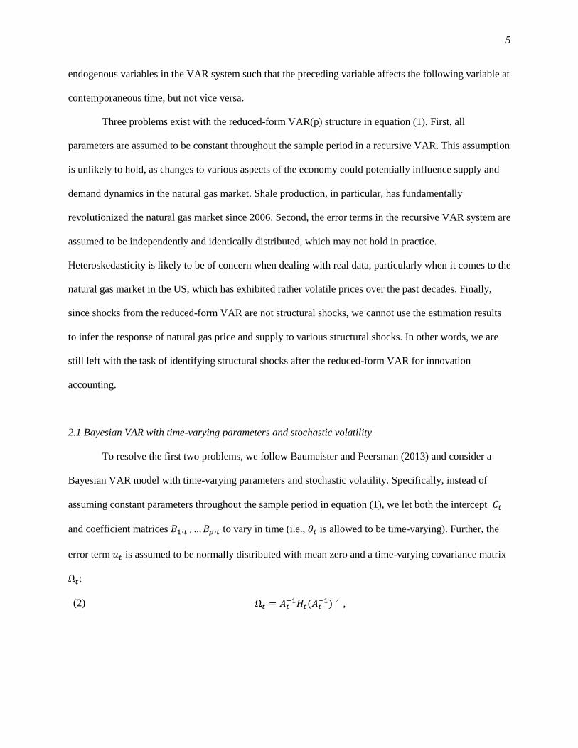
2.1 Bayesian VAR with time-varying parameters and stochastic volatility
To resolve the first two problems, we follow Baumeister and Peersman (2013) and consider a
Bayesian VAR model with time-varying parameters and stochastic volatility. Specifically, instead of
assuming constant parameters throughout the sample period in equation (1), we let both the intercept 𝐶𝑡
and coefficient matrices 𝐵1,𝑡 , …𝐵𝑝,𝑡 to vary in time (i.e., 𝜃𝑡 is allowed to be time-varying). Further, the
error term 𝑢𝑡 is assumed to be normally distributed with mean zero and a time-varying covariance matrix
Ω𝑡:
(2) Ω𝑡 = 𝐴𝑡−1𝐻𝑡(𝐴𝑡
−1)′,
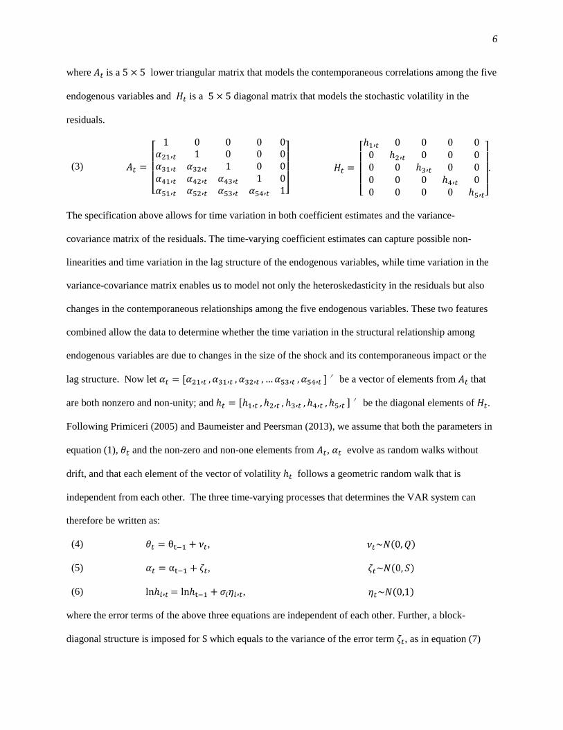
6
where 𝐴𝑡 is a 5 × 5 lower triangular matrix that models the contemporaneous correlations among the five
endogenous variables and 𝐻𝑡 is a 5 × 5 diagonal matrix that models the stochastic volatility in the
residuals.
(3) 𝐴𝑡 =
[
1 0 0 0 0𝛼21,𝑡 1 0 0 0𝛼31,𝑡 𝛼32,𝑡 1 0 0𝛼41,𝑡 𝛼42,𝑡 𝛼43,𝑡 1 0𝛼51,𝑡 𝛼52,𝑡 𝛼53,𝑡 𝛼54,𝑡 1]
𝐻𝑡 =
[ ℎ1,𝑡 0 0 0 00 ℎ2,𝑡 0 0 00 0 ℎ3,𝑡 0 00 0 0 ℎ4,𝑡 00 0 0 0 ℎ5,𝑡]
.
The specification above allows for time variation in both coefficient estimates and the variance-
covariance matrix of the residuals. The time-varying coefficient estimates can capture possible non-
linearities and time variation in the lag structure of the endogenous variables, while time variation in the
variance-covariance matrix enables us to model not only the heteroskedasticity in the residuals but also
changes in the contemporaneous relationships among the five endogenous variables. These two features
combined allow the data to determine whether the time variation in the structural relationship among
endogenous variables are due to changes in the size of the shock and its contemporaneous impact or the
lag structure. Now let 𝛼𝑡 = [𝛼21,𝑡 , 𝛼31,𝑡 , 𝛼32,𝑡 , …𝛼53,𝑡 , 𝛼54,𝑡 ]′ be a vector of elements from 𝐴𝑡 that
are both nonzero and non-unity; and ℎ𝑡 = [ℎ1,𝑡 , ℎ2,𝑡 , ℎ3,𝑡 , ℎ4,𝑡 , ℎ5,𝑡 ]′ be the diagonal elements of 𝐻𝑡.
Following Primiceri (2005) and Baumeister and Peersman (2013), we assume that both the parameters in
equation (1), 𝜃𝑡 and the non-zero and non-one elements from 𝐴𝑡, 𝛼𝑡 evolve as random walks without
drift, and that each element of the vector of volatility ℎ𝑡 follows a geometric random walk that is
independent from each other. The three time-varying processes that determines the VAR system can
therefore be written as:
(4) 𝜃𝑡 = θt−1 + 𝜈𝑡, 𝜈𝑡~𝑁(0, 𝑄)
(5) 𝛼𝑡 = αt−1 + 𝜁𝑡, 𝜁𝑡~𝑁(0, 𝑆)
(6) lnℎ𝑖,𝑡 = lnℎt−1 + 𝜎𝑖𝜂𝑖 ,𝑡, 𝜂𝑡~𝑁(0,1)
where the error terms of the above three equations are independent of each other. Further, a block-
diagonal structure is imposed for S which equals to the variance of the error term 𝜁𝑡, as in equation (7)

7
(7)
21,
1 1 1 1 2 1 3
21,
2 1 2 2 3 2 4
21,
3 1 3 2 3 3 4
4 1 4 2 4 3 4
21,
0 0 0
0 0 0( )
0 0 0
0 0 0
t
t
tt
t
S
SS Var Var
S
S
where 𝑆1 ≡ 𝑉𝑎𝑟(𝜁21,𝑡 ), 𝑆2 ≡ 𝑉𝑎𝑟([𝜁31,𝑡 , 𝜁32,𝑡 ]′), 𝑆3 ≡ 𝑉𝑎𝑟([𝜁41,𝑡 , 𝜁42,𝑡 , 𝜁43,𝑡 ]′ ), 𝑆3 ≡
𝑉𝑎𝑟([𝜁41,𝑡 , 𝜁42,𝑡 , 𝜁43,𝑡 ]′ ), and 𝑆4 ≡ 𝑉𝑎𝑟([𝜁51,𝑡 , 𝜁52,𝑡 , 𝜁53,𝑡 , 𝜁54,𝑡 ]′ ). This implies that the nonzero and
non-unity elements in matrix 𝐴𝑡 in each row evolve independently from elements of other rows. Since 𝐴𝑡
are the parameters that model the contemporaneous correlations among the five endogenous variables,
imposing a block-diagonal structure on S essentially implies that the shocks of the contemporaneous
correlations are correlated within, but not across, equations.
Following Baumeister and Peersman (2013), the VAR model with time-varying parameters and
stochastic volatility can be estimated using the Bayesian methods of Kim and Nelson (1999). Details of
the estimation procedure can be found in Baumeister and Peersman (2013).
2.2 Identifying structural shocks with sign restrictions
The third problem associated with the recursive VAR system as in equation (1) is that the
response of endogenous variables 𝑦𝑡 to the error term 𝑢𝑡 are in general not structural shocks. By
construction, a structural VAR system requires the recovery of parameters in the matrix that specifies the
contemporaneous relationship among endogenous variables. Kilian (2011) summarizes various
approaches that can be used to identify structural shocks, including institutional knowledge, economic
theory, other extraneous constraints on the model responses, sign restrictions, etc.
Following Arora (2014), we impose the following sign restrictions to identify the structural
shocks (table 1):

8
Table 1. Sign Restrictions
𝐐 𝐏 𝐈 𝐑 𝐕
Natural gas supply shock + - + +
Residual shock +
Industrial demand shock + + +
Residential demand shock + + + -
Precautionary inventory demand shock + + - +
Notes: Q is the total available natural gas supply in the US, P is the price of natural gas, I is the industrial demand, R
is the residential demand, and V is the precautionary inventory demand. All shocks are assumed to be positive.
A positive shock in the available natural gas supply is likely to induce a negative response in
natural gas prices. A readily available example is the recent expansion of shale gas production that has
shifted the natural gas supply curve to the right, and moving the real price of natural gas to the opposite
direction. The response of natural gas price to positive supply shocks is thus restricted to be non-positive.
On the other hand, positive supply shocks are associated with increased supply of natural gas in the
market, as well as increased residential and industrial demand. We do not impose any sign restriction for
the impact of supply shocks on the precautionary demand of inventory.
A positive shock on industrial demand driven by the aggregate economic activity in the US is
assumed to increase the total supply of natural gas in the market, the real price of natural gas, as well as
the industrial demand. No sign restrictions are placed on the response of residential demand or
precautionary inventory demand to a positive shock on industrial demand. Similarly, a positive shock on
residential demand of natural gas is expected to induce a positive response at contemporaneous time on
the total supply of natural gas, the real price of natural gas, and the residential demand. It should also
result in a negative response to the precautionary demand as inventory is likely to decline when more
natural gas is used for residential consumption.
For storable commodities, the level of inventory available in the system partly reflects how
quickly firms can respond to unexpected demand and supply shocks. The theory of storage (e.g., Brennan,

9
1958, Kaldor, 1939, Working, 1949, Working, 1948) states that firms earn a convenience yield by holding
inventory at hand, which prevents disruptions in the flow of goods and services, and in turn reduces
production uncertainty. A number of studies have investigated the relationship between prices and
inventories (e.g., Miranda and Fackler, 2004, Wright, 2011, Wright and Williams, 1991), showing that
inventories can help absorb price fluctuations. During periods of high prices, storage holders can sell out
inventories that incur high opportunity costs, effectively lowering price levels. On the other hand, storage
holders can replenish inventories when prices are low, helping again to buffer prices. The implication is
that a positive unanticipated shock on precautionary demand of inventory will induce a positive response
in the real price of natural gas, as there is a greater demand of natural gas during the current period.
Supply and inventory are also assumed to increase after a positive shock on precautionary demand of
inventory, while the response of industrial demand driven by aggregate economic activity is assumed to
be negative. The latter sign restriction implies that the demand for natural gas used in industrial
production is likely to decline following a positive shock on the speculative demand.
Finally, we assume that a positive residual shock will induce a positive response of real natural
gas prices. We do not, however, impose any sign restrictions on the response of other variables.
3. Data
The data used in this study follows Arora (2014) closely. Natural gas prices are from the Producer
Price Index published by the Bureau of Labor Statistics, and October 1982 is used as the baseline.1 To
model the supply of natural gas, we use the marketed US natural gas production published by the EIA.2 In
the process of natural gas production, marketed natural gas refers to the gas produced before associated
liquids such as propane and butane are extracted. The definition should be distinguished from dry natural
1 Under the Fuels and related products and power group on the Bureau of Labor Statistics website, the item Natural
gas is used. See http://data.bls.gov/timeseries/WPU0531
2 The marketed US natural gas production data is published by the EIA in monthly intervals in millions of cubic
feet. See http://www.eia.gov/dnav/ng/hist/n9010us2m.htm

10
gas, which refers to the gas when these liquids are removed. Here the marketed amount is used rather than
the gross amount as a measure of natural gas supply so that any gas consumed either in extraction or
processing is ignored.
We model the demand of natural gas using three variables, total demand of natural gas from
industrial production, residential demand, and precautionary inventory demand of natural gas. Total
industrial production measures the demand for natural gas driven by changes in US economic activity,
and thus provide a measure of the business cycle driven by the aggregate economic activity. As such,
shocks to the industrial demand of natural gas may be interpreted as the aggregate economic activity
shock. The Federal Reserve publishes an index of industrial production and capacity utilization (G.17),
which is used as a proxy for the industrial demand of natural gas in the US.3 A second dimension of
natural gas demand comes from the residential side. Residential demand accounts for a substantial
fraction of the natural gas in the US. Using data from EIA, it is estimated that in 2013 over 20 percent of
the total natural gas use in the US was for residential purposes. Data on residential natural gas demand are
obtained from the EIA as well.4 Lastly, we use the EIA natural gas inventory data as a measure of
precautionary inventory demand.5 For storable commodities like natural gas, inventory reflects
expectation of future supply and demand and storage expands when the expected future price exceeds the
current period price plus storage cost and convenience yield. Kilian and Murphy further argue that the
inventory demand may also be interpreted as speculative demand as speculators tend to put more
commodity into storage if they expect a substantial rise in future prices.
The data period begins on January 1976 and ends on August 2014, and is sampled at a monthly
frequency. In the US, the federal government has regulated the natural gas market for many years. The
Natural Gas Act of 1938 gave the Federal Power Commission the authority to regulate gas rates. This
3 Available at http://www.federalreserve.gov/releases/g17/download.htm
4 See http://www.eia.gov/totalenergy/data/monthly/#naturalgas
5 See http://www.eia.gov/naturalgas/data.cfm#storage

11
continued until passage of the Natural Gas Policy Act (NGPA) of 1978, which created the Federal Energy
Regulatory Commission (FERC). The NGPA was the first effort to deregulate the natural gas market, but
Congress passing the Natural Gas Wellhead Decontrol Act was the main driver. All price regulations
were eliminated by January 1993. Combined with FERC order 636, mandating the unbundling of pipeline
services (previously pipelines were able to combine sales and transportation), this act of Congress
effectively ended all government control over the market.
Given the history of federal regulation of the natural gas market, we use data from 1976 to 1992
for burn-in iterations in the Bayesian VAR model with time-varying parameters and stochastic volatility
as outlined in section two, and use the data from January 1993 to August 2014 for time series analyses.
Figure 1 plots the five variables used in the analysis. As can be seen, the supply of natural gas
was relatively stable between 1990 and 2005, after which the production quickly took off, growing more
than 40 percent from 2006 to 2014. This rapid growth largely reflects the expansion of shale gas
production due to the popularization of the combined use of horizontal drilling and hydraulic fracturing
techniques. The natural gas producer price index (panel (b) of figure 1) shows that much variation in
natural gas prices has occurred since 1993, when all price regulations on natural gas in the US were
eliminated. Further, the expansion of shale gas production has resulted in a rather low level of natural gas
prices. Panel (c) of figure 1 shows the US industrial production index. With one setback in 2002 and
another in 2008, the industrial production index, reflecting the aggregate economic activity in the US, has
been growing at a rather steady rate. Both residential demand (panel (d) of figure 1) and precautionary
inventory demand (panel (e) of figure 1) show a significant degree of seasonality, partly due to the fact
that natural gas is used primary in winter seasons for space heating in residential homes.

12
Figure 1. US Natural Gas Supply and Demand, January 1976 – August 2014
Jan75 Jan80 Jan85 Jan90 Jan95 Jan00 Jan05 Jan10 Jan151
1.5
2
2.5
Mil
lio
n M
Mcf
(a) Marketed Natural Gas Production in the US
Jan75 Jan80 Jan85 Jan90 Jan95 Jan00 Jan05 Jan10 Jan150
200
400
600
Ind
ex
(b) Natural Gas Producer Price Index
Jan75 Jan80 Jan85 Jan90 Jan95 Jan00 Jan05 Jan10 Jan1540
60
80
100
120
Ind
ex
(c) US Industrial Production Index
Jan75 Jan80 Jan85 Jan90 Jan95 Jan00 Jan05 Jan10 Jan150
500
1000
1500
Bil
lio
n c
ub
ic f
eet
(d) US Residential Natural Gas Demand
Jan75 Jan80 Jan85 Jan90 Jan95 Jan00 Jan05 Jan10 Jan154
6
8
10
Mil
lio
n M
Mcf
(e) US Natural Gas Underground Storage

13
Table 2 reports the results from augmented Dickey-Fuller (ADF) and Phillips-Perron (PP) tests
both with and without a trend for the five variables used in the analysis. All variables have been
transformed to logarithmic form. The lag length of the ADF test is selected using the Akaike information
criterion (AIC). As can be seen, with the exception of industrial demand, all of the other four variables
appear to be non-stationary in levels using the ADF test both with and without a trend. Using the PP test
without a trend, the industrial demand and inventory demand are considered to be stationary. In addition
to these two variables, the real price of natural gas is also considered to be stationary when using the PP
test with a trend. All five variables appear to be stationary in first differences.
Table 2. Unit Root Test Results
---------In Logarithmic Levels------ --First Diff---
No Trend With Trend
ADF PP ADF PP ADF
Supply -2.21 -2.32 -2.44 -2.72 -7.04 ***
Real Price 1.15 -2.34 -0.21 -5.98 *** -6.65 ***
Industrial Demand -14.86 *** -6.84 *** -12.29 *** -6.85 *** -17.50 ***
Residential Demand -2.20 -2.06 -2.13 -2.27 -4.47 ***
Inventory Demand -1.53 -6.05 *** -1.77 -6.42 *** -11.95 ***
Notes: ADF refers to augmented Dickey-Fuller test, PP refers to Phillips-Perron test. One, two, and three asterisks refers to a signficance level at
10, 5, and 1 percent, respectively.
Given the mixed results from the unit root test for the five variables in levels, we consider their
first differences, which essentially measure the monthly growth rate of each variable.
4. Empirical Results
In this section, we report results from the VAR analysis. First, we use the recursive structure to
obtain the constant-coefficient point estimates, and then discuss the results of the Bayesian VAR model
with time-varying parameters and stochastic volatility. A comparison between the results from these two
models highlights the importance of accounting for time-variation, stochastic volatility, and sign
restrictions when modeling natural gas prices.

14
4.1 Recursive VAR results
The key assumption underlying a recursive VAR model is that no variable is affected by the
variable that follows at contemporaneous time. We impose the recursive structure as in equation (8):
(8)
natural gas supply shock11
aggregate demand shock21 22
residential demand shock31 32 33
precautionary d41 42 43 44
51 52 53 54 55
0 0 0 0
0 0 0
0 0
0
Q
t t
I
t t
Rt t t
V
t t
P
t
au
a au
u a a au
a a a au
a a a a au
emand shock
residual shock
t
where tu are the residuals from the reduced-form model as in equation (1) associated with each
individual equation, Q, I, R, V, and P are the total supply of natural gas, industrial demand, residential
demand, inventory demand, and real natural gas prices, respectively. t are the structural shocks.
The recursive structure imposes a vertical short-run supply curve of natural gas such that natural
gas supply is not affected contemporaneously by any demand-side shocks but by unanticipated natural gas
supply shocks only. The justification of placing natural gas supply as the first variable in the system
follows from Kilian (2009, 2011) who argues that the supply of natural gas is unlikely to respond to
demand shocks in an instantaneous fashion (here, within one month) as it takes certain amount of time for
natural gas producers to react to any unanticipated change in industrial, residential, or inventory demand.
Such an exclusion restriction has been frequently used in the literature as a way to identify structural
shocks (e.g. Kilian 2009).
Innovations to aggregate economic activity that cannot be explained by natural gas supply shocks
are referred to as shocks to the aggregate demand for industrial commodities in the US, and are
considered to contemporaneously affect residential demand and inventory demand in addition to the real
price of natural gas, but not vice versa. This means that increases in the residential demand and inventory
demand of natural gas, as well as the real price of natural gas, are unlikely to induce an instantaneous
response (here, within one month) in the aggregate economic activity in the US.

15
Residential demand is the third variable in the system. Innovations to residential demand that
cannot be explained by either natural gas supply shocks or aggregate demand shocks are referred to as
shocks to the residential demand of natural gas. As residential demand only represents a small portion of
the US market for natural gas, and that residential demand has remained stable during the sample period
(effect of energy efficiency is offset by the increase in total number of consumers), an unexpected shock
in the precautionary inventory demand or the real price of natural gas is unlikely to induce a response in
the residential demand within one month.
The final two variables are ordered as inventory demand and real price of natural gas. These are
innovations to inventory demand and real price of natural gas that cannot be explained by the previous
three structural shocks, namely supply shocks, aggregate demand shocks, and residential demand shocks.
We assume that in the short-run, an unexpected shock in the real price of natural gas will not induce an
immediate response in the precautionary inventory demand. One possibility is that the storage facility is
not readily available at the time the shock in the real price occurs.
The recursive VAR as postulated in equation (8) can be consistently estimated using conventional
estimation procedures. A lag length of two is selected based on AIC, and to account for seasonality, we
also include monthly dummies as exogenous variables in the system. We first report the impulse response
functions, focusing on the response of supply and price of natural gas to the five structural shocks, and
then report the forecast error variance decomposition.
Impulse response functions display reactions of each variable to unexpected shocks to the model,
and for how long those effects persist. Figure 2 shows the cumulative responses of total natural gas
supply and prices to the five structural shocks considered in this study at a two-year horizon, where the 95
percent confidence intervals are obtained through bootstraps with 1,000 replications. Focusing first on the
response of supply to various structural shocks (top row of figure 2). As can be seen, an unanticipated
supply shock has a large positive impact on total natural gas supply in the US. Speculative demand
shocks induce a negative response in the total supply of natural gas in the US. The responses of natural
gas supply to other three shocks are not statistically significant.

16
Figure 2. Cumulative Response of Natural Gas Supply (Top Row) and Natural Gas Prices (Bottom Row) to a Structural Shock
Responses of natural gas prices to various structural shocks (bottom row of figure 2) show a
rather different pattern. Shocks to residential demand have only a small effect on prices, and the
cumulative response of prices is never statistically significant. Industrial production shocks have a large
and positive effect on prices, as higher macro-economic activity increases demand. Inventory shocks have
a large and negative effect on prices. One possibility is that as inventory increases, the expected future
supply of natural gas increases as well, thus effectively lowering the prices in subsequent periods. Natural
gas production shocks overall have a negative effect on prices. However, the cumulative response is not
significant after five months.
Table 3 presents the forecast error variance decomposition for supply and real price of natural
gas. Each cell in the table represents the percentage of the forecast error in one variable induced by
developments in another variable. As can be seen, the majority of the forecast error variance of supply
can be explained by shocks to the supply. Even at the two-year horizon, shocks to the supply contribute to
as much as 90 percent of the total forecast error variance. Speculative demand shocks come as the second
most important variable, accounting for 4.5 percent of the forecast error variance for supply. Industrial
0 10 20
0.4
0.5
0.6
0.7
0.8
0.9
1
Res
po
nse
(a) Supply Shock
0 10 20-0.8
-0.6
-0.4
-0.2
0
0.2
0.4
0.6
Res
po
nse
(b) Aggregate Demand Shock
0 10 20-0.12
-0.1
-0.08
-0.06
-0.04
-0.02
0
0.02
0.04
Res
po
nse
(c) Residential Demand Shock
0 10 20-0.8
-0.7
-0.6
-0.5
-0.4
-0.3
-0.2
-0.1
0
0.1
0.2
Res
po
nse
(d) Speculative Demand Shock
0 10 20-0.04
-0.03
-0.02
-0.01
0
0.01
0.02
0.03
0.04
Res
po
nse
(e) Residual Shock
0 10 20-4.5
-4
-3.5
-3
-2.5
-2
-1.5
-1
-0.5
0
0.5
Res
po
nse
(a) Supply Shock
0 10 20-2
0
2
4
6
8
10
Res
po
nse
(b) Aggregate Demand Shock
0 10 20-0.8
-0.6
-0.4
-0.2
0
0.2
0.4
0.6
Res
po
nse
(c) Residential Demand Shock
0 10 20-9
-8
-7
-6
-5
-4
-3
-2
-1
0
Res
po
nse
(d) Speculative Demand Shock
0 10 200.4
0.5
0.6
0.7
0.8
0.9
1
1.1
Res
po
nse
(e) Residual Shock

17
demand shocks contribute to 3.2 percent of the error variance at the end of the two-year horizon. Residual
and residential demand shocks appear to explain only a negligible portion of the forecast error variance.
Figure 3. Median Short-Run Price Elasticities of Natural Gas Supply and Demand from 1993 to 2014
Results of forecast error variance decomposing on real natural gas prices show a bigger
contribution from other structural shocks. Innovations in industrial production explain a small share of
1994 1996 1998 2000 2002 2004 2006 2008 2010 2012 20140
0.2
0.4
0.6
0.8
(a) Natural Gas Supply Elasticity with Aggregate Demand Shock
1994 1996 1998 2000 2002 2004 2006 2008 2010 2012 20140
0.1
0.2
0.3
0.4
(b) Natural Gas Supply Elasticity with Residential Demand Shock
1994 1996 1998 2000 2002 2004 2006 2008 2010 2012 20140
0.5
1
1.5
(c) Natural Gas Supply Elasticity with Inventory Demand Shock
1994 1996 1998 2000 2002 2004 2006 2008 2010 2012 20140
0.5
1
(d) Natural Gas Supply Elasticity with other Natural Gas Demand Shock
1994 1996 1998 2000 2002 2004 2006 2008 2010 2012 2014-0.8
-0.6
-0.4
-0.2
0
(e) Natural Gas Demand Elasticity

18
price variations. This suggests producing firms have some degree of flexibility in their production. When
changes in industrial production occur, they appear to have some ability to adjust their production to
match economic output. Natural gas production changes explain the some variation in prices, which is a
predictable result consistent with economic theory. Innovations in residential demand have a non-trivial
effect on prices, explaining approximately 6-8% at the end of each time period. Inventories account for a
large share of price variation, between 11-13%. Capacity constraints could be one possible explanation, in
that if inventories were high (indicating a high utilization capacity of available storage inventories), a
sudden rise in the amount of natural gas stored in inventories could account for a much larger share of
price variation than if inventories were lower. Finally, at the end of a two-year horizon, residual shocks
account for approximately two thirds of the total forecast error variance of real prices.
Forecast error variance decomposition on other variables (results not presented) shows that
innovations in natural gas prices have only small effects on residential demand, supporting the well-
established theory of inelastic demand for energy sources. Prices do have a larger effect on industrial
production, suggesting a strong dependence on commodity prices. Inventories are effected by other
natural gas market shocks (residual shocks), but only after a lag-time of two months.
Overall, results from the recursive VAR model suggest that unanticipated supply shocks are the
primary driver of the total supply of natural gas in the US, followed by speculative demand shocks and
aggregate demand shocks from 1993 to 2014. Shocks to residential demand and residual shocks only
contribute minimally to the supply of natural gas. Results on natural gas prices showed a much bigger
role of other variables, in that the response of prices to aggregate demand, speculative demand, and
supply shocks are all statistically significant. The role of residential demand shocks, however, remains
negligible.

19
Table 3. Forecast Error Variance Decomposition from the Rucursive VAR Model
Months
Supply
Shocks
Aggregate
Demand Shocks
Residential
Demand Shocks
Inventory Demand
Shocks
Other Natural Gas
Demand Shocks
Panel A. Natural Gas Supply
1 100.00% 0.00% 0.00% 0.00% 0.00%
3 95.80% 1.07% 0.10% 2.72% 0.31%
5 90.57% 3.13% 0.89% 4.51% 0.91%
9 89.91% 3.20% 1.39% 4.51% 1.00%
12 89.87% 3.19% 1.41% 4.51% 1.01%
15 89.87% 3.20% 1.41% 4.51% 1.01%
18 89.87% 3.20% 1.41% 4.51% 1.01%
21 89.87% 3.20% 1.41% 4.51% 1.01%
24 89.87% 3.20% 1.41% 4.51% 1.01%
Panel B. Real Price of Natural Gas
1 2.47% 5.15% 1.06% 0.18% 91.15%
3 3.96% 5.40% 8.03% 12.25% 70.36%
5 4.07% 6.54% 7.93% 13.22% 68.24%
9 4.41% 6.61% 8.03% 13.24% 67.72%
12 4.41% 6.61% 8.04% 13.24% 67.71%
15 4.41% 6.61% 8.04% 13.24% 67.70%
18 4.41% 6.61% 8.04% 13.24% 67.70%
21 4.41% 6.61% 8.04% 13.24% 67.70%
24 4.41% 6.61% 8.04% 13.24% 67.70%
4.2 Structural Model
In this section, we discuss the results from the Bayesian VAR model with time-varying
parameters and stochastic volatility.
Figure 3 presents the evolution of median short-run price elasticities in natural gas supply and
demand over the sample period. Given that we include three dimensions of oil demand, namely industrial
demand driven by aggregate economic activity, residential demand, and precautionary inventory demand,
we trace the curvature of the natural gas supply elasticity with all these three shocks, as well as the

20
residual shocks associated with the real price of natural gas. As can be seen, the median supply elasticity
associated with aggregate economic demand ranges from 0.09 to 0.78, with the largest value occurring at
the beginning of the sample period (1993-1995). The supply elasticity gradually declines starting from
mid-1995. It is not until 1998 that the natural gas supply curve becomes more elastic. During 1999-2004,
the median supply elasticity associated with aggregate demand shock ranges from 0.09 to 0.25, indicating
a rather insensitive supply response to industrial demand shocks driven by aggregate economic activity.
The implication is that natural gas supply is unlikely to significantly increase even with rapid economic
growth. One possible explanation is that, due to technology constraints, producers are unable to increase
production significantly and take advantage of the fast-growing economy, but have to instead maintain
the current level of production. With the popularization of the combined use of horizontal drilling and
hydraulic fracturing techniques, supply has apparently become much more responsive to aggregate
demand shocks, with the median impact elasticity ranging from 0.2 to 0.6 between 2004 and 2014. In
particular, a particularly rapid increase in supply elasticity is observed starting from 2009, when the
economy in the US starts to recover from the 2008 financial crisis.
A rather similar pattern exists for the supply elasticity associated with residential demand shock,
though with much smaller magnitudes. The median supply elasticity ranges from 0.1 to 0.38, suggesting
that the supply of natural as in the US is much less responsive to residential demand shock, as compared
to industrial demand shock driven by aggregate economic activity. This is consistent with the observation
that residential demand accounts for a much smaller portion of the total natural gas use compared to
industrial demand. The supply curve appears to be more elastic for the first few years of the sample
period, with the median impact elasticity ranging from 0.2 to 0.38. Starting from 1998, the supply
elasticity associated with residential demand shock remained at a low level until 2004, often fluctuating
between 0.1 and 0.2. 2006 marks the first time over the past decade that the supply elasticity has gone
beyond 0.3. Though it subsided a bit afterwards, the supply elasticity quickly increases starting from
2008, a pattern similar to the supply curve with aggregate demand shocks.

21
The evolution of supply elasticity with inventory demand shocks over the sample period are
presented in panel (c) of figure 3. As can be seen, much larger variations are observed for the first ten
years of the sample (1993-2003), with the median supply elasticity ranging from 0.2 to 1.2. By contrast,
the curvature of the supply curve associated with precautionary inventory demand has remained
somewhat steady starting from 2005, ranging from 0.3 to 0.6. The implication is that with one percentage
of unanticipated precautionary inventory demand shock, the supply of natural gas is likely to increase by
0.3 to 0.6 percent from 2005 to 2014.
The fourth panel of figure 3 shows the supply elasticity with other natural gas demand shocks that
cannot be explained by unanticipated supply shocks, aggregate demand shocks, residential demand
shocks, or speculative demand shocks. It appears that the supply curve is most elastic during the
beginning and end of the sample period. The supply elasticity associated with this type of residual shock
ranges from 0.3 to 1.0. For most months in the 1995-2011 sample period, the supply elasticity appears to
fluctuate around 0.5.
Panel (d) of figure 3 plots the natural gas demand elasticity. The demand elasticity ranges from -
0.5 to -0.1 over the sample period. Notably, while the demand elasticity remained rather steady from 1998
to 2008 (fluctuating around -0.2), the demand curve becomes much more elastic after 2008. One possible
explanation is that there is a greater flexibility in energy substitution such that industrial, commercial, and
residential users can switch among different fuel sources much more easily.
Given the short-run price elasticities presented in figure 3, we further compute the average
underlying shocks associated with each variable, the results of which are shown in figure 4. As can be
seen from the graph, much larger structural shocks are observed for the three demand side variables
(industrial demand, residential demand, and precautionary inventory demand shocks) during the latter part
of the sample period (2008-2014). The magnitude of each structural shock peaks between 2008 and 2010,
after which a gradual decline is observed. By contrast, the size of other natural gas market demand shocks
(or residual shocks) has become smaller in the latter part of the sample, partly reflecting a lower natural
gas price level due to the shale boom that took off in 2006.

22
Figure 4. Median Magnitude of Structural Shocks
Overall, our estimation results from the VAR model with time-varying parameters and stochastic
volatility suggest that the supply curve associated with aggregate demand shocks, residential demand
1994 1996 1998 2000 2002 2004 2006 2008 2010 2012 20141.5
2
2.5
3
3.5
4
(b) Aggregate Demand Shock
1994 1996 1998 2000 2002 2004 2006 2008 2010 2012 20141.5
2
2.5
3
3.5
4
4.5
(c) Residential Demand Shock
1994 1996 1998 2000 2002 2004 2006 2008 2010 2012 20141.5
2
2.5
3
3.5
4
(d) Precautionary Inventory Demand Shock
1994 1996 1998 2000 2002 2004 2006 2008 2010 2012 20141.5
2
2.5
3
(e) Other Natural Gas Demand Shock

23
shocks, and other natural gas market demand shocks has become more elastic during the latter part of the
sample. This is also the period that marks the rapid expansion in shale gas production. By contrast, the
curvature of the supply curve associated with precautionary inventory demand shocks has remained at a
stable level for most part of the sample since 2000, and has not changed much even in the face of rapid
production growth driven by the shale gas boom. Furthermore, it appears that in the new era characterized
with ample natural gas supply, the demand curve has also become more elastic, partly reflecting the fact
that there is a greater flexibility of substitution in fuel use.
5. Conclusions
In this paper, we disentangle supply and demand shocks on US natural gas prices and investigate
how these effects have changed over time. Whereas most previous studies have only used reduced-form
analyses, this paper uses a structural vector autoregressive model (SVAR) to examine price dynamics
under a theoretically-driven structural framework. Unlike Wakamatsu and Aruga (2013) and Arora
(2014), who all impose a one-time arbitrary structural break, we generate a time-varying parameter model
that allows the data to determine when and how any changes may have occurred. To this end, we
construct a long sample period that not only includes both the pre-and post- shale boom (1976-2014), but
also uses a new identification strategy recently developed by Baumeister and Peersman (2013), allowing
for drifting coefficients and stochastic volatility in the SVAR model.
Results from the recursive VAR model suggest that unanticipated supply shocks is the primary
driver of the total supply of natural gas in the US, followed by speculative demand shocks and aggregate
demand shocks during 1993-2014. Shocks to residential demand and residual shocks only contribute
minimally to the supply of natural gas. In fact, results on natural gas prices show that other variables play
a much bigger role, in that the response of prices to aggregate demand, speculative demand, and supply
shocks are all statistically significant. The role of residential demand shocks, however, remains
negligible.

24
Our results from the VAR model with time-varying parameters and stochastic volatility suggest
that the supply curve associated with aggregate demand shocks, residential demand shocks, and other
natural gas market demand shocks has all become more elastic during the latter part of the sample. This is
commensurate with the period of rapid expansion in shale gas production. By contrast, the curvature of
the supply curve associated with precautionary inventory demand shocks has remained at a stable level
for most of the sample since 2000, and has not changed much even with the rapid growth of shale gas
production. Furthermore, it appears that in the new era characterized with ample natural gas supply, the
demand curve has also become more elastic, partly reflecting the fact that there is a greater flexibility of
substitution in fuel use.

25
References
Arora, V. "Estimates of the price elasticities of natural gas supply and demand in the United States."
MPRA Paper No. 54232. Available at http://mpra.ub.uni-muenchen.de/54232/. .
Atil, A., A. Lahiani, and D.K. Nguyen. 2014. "Asymmetric and nonlinear pass-through of crude oil prices
to gasoline and natural gas prices." Energy Policy 65:567-573.
Baumeister, C., and G. Peersman. 2013. "The Role of Time‐Varying Price Elasticities in Accounting for
Volatility Changes in the Crude Oil Market." Journal of Applied Econometrics 28:1087-1109.
---. 2013. "Time-Varying Effects of Oil Supply Shocks on the US Economy." American Economic
Journal: Macroeconomics 5:1-28.
Bistline, J.E. 2014. "Natural gas, uncertainty, and climate policy in the US electric power sector." Energy
Policy 74:433-442.
Brennan, M.J. 1958. "The supply of storage." The American Economic Review:50-72.
Brigida, M. 2014. "The switching relationship between natural gas and crude oil prices." Energy
Economics 43:48-55.
Cogley, T., and T.J. Sargent. 2005. "Drifts and volatilities: monetary policies and outcomes in the post
WWII US." Review of Economic dynamics 8:262-302.
Hartley, P.R., and Medlock, Kenneth B. 2014. "The relationship between crude oil and natural gas prices:
The role of the exchange rate." The Energy Journal 32.
Ji, Q., J.-B. Geng, and Y. Fan. 2014. "Separated influence of crude oil prices on regional natural gas
import prices." Energy Policy 70:96-105.
Kaldor, N. 1939. "Speculation and economic stability." The Review of Economic Studies 7:1-27.
Kilian, L. 2009. "Not All Oil Price Shocks Are Alike: Disentangling Demand and Supply Shocks in the
Crude Oil Market." American Economic Review 99:1053-1069.
---. "Structural Vector Autoregressions." CEPR Discussion Papers.
Kilian, L., and D.P. Murphy. 2014. "The role of inventories and speculative trading in the global market
for crude oil." Journal of Applied Econometrics 29:454-478.

26
Kim, C.-J., and C.R. Nelson. 1999. "Has the US economy become more stable? A Bayesian approach
based on a Markov-switching model of the business cycle." Review of Economics and Statistics
81:608-616.
Miranda, M.J., and P.L. Fackler. 2004. Applied Computational Economics and Finance. Cambridge, MA:
MIT press.
Mohammadi, H. 2011. "Long-run relations and short-run dynamics among coal, natural gas and oil
prices." Applied economics 43:129-137.
Mu, X. 2007. "Weather, storage, and natural gas price dynamics: Fundamentals and volatility." Energy
Economics 29:46-63.
Nick, S., and S. Thoenes. 2014. "What drives natural gas prices?—A structural VAR approach." Energy
Economics 45:517-527.
Olsen, K.K., J.W. Mjelde, and D.A. Bessler. 2014. "Price formulation and the law of one price in
internationally linked markets: an examination of the natural gas markets in the USA and
Canada." The Annals of Regional Science:1-26.
Park, H., J.W. Mjelde, and D.A. Bessler. 2007. "Time-varying threshold cointegration and the law of one
price." Applied economics 39:1091-1105.
Primiceri, G.E. 2005. "Time varying structural vector autoregressions and monetary policy." The Review
of Economic Studies 72:821-852.
Qin, X., et al. (2010) "Fundamentals and US natural gas price dynamics." In 2010 Annual Meeting,
February 6-9, 2010, Orlando, Florida. Southern Agricultural Economics Association.
Ramberg, D.J., and J. Parsons, E. 2012. "The Weak Tie Between Natural Gas and Oil Prices." The Energy
Journal 33.
Renou-Maissant, P. 2012. "Toward the integration of European natural gas markets: A time-varying
approach." Energy Policy 51:779-790.
Siliverstovs, B., et al. 2005. "International market integration for natural gas? A cointegration analysis of
prices in Europe, North America and Japan." Energy Economics 27:603-615.

27
Trembath, A., et al. 2012. "US Government Role in Shale Gas Fracking History: An Overview and
Response to Our Critics." The Breakthrough, March 2.
US EIA (2015). Annual Energy Outlook 2015. Available at:
http://www.eia.gov/forecasts/AEO/pdf/0383(2015).pdf.
Wakamatsu, H., and K. Aruga. 2013. "The impact of the shale gas revolution on the US and Japanese
natural gas markets." Energy Policy 62:1002-1009.
Working, H. 1949. "The Theory of Price of Storage." American Economic Review 39:1254-1262.
---. 1948. "Theory of the inverse carrying charge in futures markets." Journal of Farm Economics 30:1-
28.
Wright, B.D. 2011. "The Economics of Grain Price Volatility." Applied Economic Perspectives and
Policy 33:32-58.
Wright, B.D., and J.C. Williams. 1991. Storage and Commodity Markets. Cambridge, UK: Cambridge
University Press.