u.s. investment in global bonds - the national …. investment in global bonds: as the fed pushes,...
TRANSCRIPT

NBER WORKING PAPER SERIES
U.S. INVESTMENT IN GLOBAL BONDS:AS THE FED PUSHES, SOME EMEs PULL
John D. BurgerRajeswari SenguptaFrancis E. Warnock
Veronica Cacdac Warnock
Working Paper 20571http://www.nber.org/papers/w20571
NATIONAL BUREAU OF ECONOMIC RESEARCH1050 Massachusetts Avenue
Cambridge, MA 02138October 2014
This paper, prepared for the 60th Panel Meeting of Economic Policy (October 2014), was lightlycirculated as "International Investors in Local Bond Markets: Indiscriminate Flows or DiscriminatingTastes?" The authors thank Sumit Malhotra for excellent research assistance, Robert DeMason ofJPMorgan for returns indices, Randolph Tantzscher of Markit for GEMLOC investabilty data, andBranimir Gruic of BIS for data on the size of local currency and USD-denominated bond markets.We also thank for helpful comments the editor (Nicola Fuchs-Schündeln), three anonymous referees,Anusha Chari, Branimir Gruic, Philip Lane, Louis Miserendino, and participants at INFINITI, AustralianConference of Economists, Banco Central de Reserva del Perú and NIPFP. Burger acknowledges aresearch sabbatical from Loyola University Maryland. The views expressed herein are those of theauthors and do not necessarily reflect the views of the National Bureau of Economic Research.
NBER working papers are circulated for discussion and comment purposes. They have not been peer-reviewed or been subject to the review by the NBER Board of Directors that accompanies officialNBER publications.
© 2014 by John D. Burger, Rajeswari Sengupta, Francis E. Warnock, and Veronica Cacdac Warnock.All rights reserved. Short sections of text, not to exceed two paragraphs, may be quoted without explicitpermission provided that full credit, including © notice, is given to the source.

U.S. Investment in Global Bonds: As the Fed Pushes, Some EMEs PullJohn D. Burger, Rajeswari Sengupta, Francis E. Warnock, and Veronica Cacdac WarnockNBER Working Paper No. 20571October 2014JEL No. F21,F31,G11
ABSTRACT
We analyze reallocations within the international bond portfolios of US investors. The most strikingempirical observation is a steady increase in US investors’ allocations toward emerging market localcurrency bonds, unabated by the global financial crisis and accelerating in the post-crisis period. Partof the increase in EME allocations is associated with global “push” factors such as low US long-terminterest rates and unconventional monetary policy as well as subdued risk aversion/expected volatility.But also evident is investor differentiation among EMEs, with the largest reallocations going to thoseEMEs with strong macroeconomic fundamentals such as more positive current account balances, lessvolatile inflation, and stronger economic growth. We also provide a descriptive analysis of globalbond markets’ structure and returns.
John D. BurgerLoyola University Maryland4501 N. Charles StreetBaltimore MD [email protected]
Rajeswari SenguptaIndira Gandhi Institute of Development Research (IGIDR)Mumbai 400 065, [email protected]
Francis E. WarnockDarden Business SchoolUniversity of VirginiaCharlottesville, VA 22906-6550and [email protected]
Veronica Cacdac WarnockDarden Business SchoolUniversity of VirginiaBox 6550Charlottesville, VA [email protected]
1
“The extent to which distortions in one country may spread to financial market developments in the other EMEs will depend to a great degree also on whether international investors look at the EMEs as a homogeneous asset class or whether they take an increasingly differentiated view in their evaluations of individual EMEs and their respective progress towards achieving macroeconomic stability. The varying reactions of bond markets in some EMEs following a rise in volatility over the last two years indicate that international investors are beginning to make a greater distinction between those countries’ bond markets depending on how the fundamentals are assessed; yet it remains to be seen whether, and to what extent, this development is a lasting one.”
Bundesbank, Financial Stability Review 2007 “…our greatest concern is financial market fragmentation…” Mario Draghi, August 2 2012
1. Introduction
Investor behavior in bond markets is of great interest to policymakers in both emerging market
economies (EMEs) and advanced economies (AEs). For EME bond markets, the Bundesbank opines that
financial stability would improve if global investors differentiated between them. In Eurozone bond
markets, the ECB equates differentiation with a fragmentation that could impede the monetary policy
transmission mechanism, suggesting that differentiation is not always and everywhere desirable. In the
background is an environment for investing in international bonds that has changed dramatically over
the past few decades with the development of EME local currency bond markets (LCBMs). EMEs with
low inflation, stronger institutions, and well defined creditor rights have experienced substantial
development of LCBMs (see Burger and Warnock 2003, 2006; Eichengreen and Luengnaruemitchai
2006, Claessens, Klingebiel, and Schmukler 2007). The ability to borrow in the local currency is a
positive development that enhances financial stability by ameliorating the currency mismatches that
were at the center of past crises (Goldstein and Turner 2004). However, large inflows of foreign
investment can be problematic, as most extreme capital flow episodes (surges and stops, for example)
are driven by debt flows (Forbes and Warnock 2013), credit booms lead to crises (Mendoza and
2
Terrones 2008, Gourinchas and Obstfeld 2012, Schularick and Taylor 2012), and large foreign
investment flows into LCBMs can complicate the tasks of EME policymakers by appreciating real
exchange rates, fanning asset price bubbles, and intensifying lending booms. Indeed, the threat of the
virtuous cycle turning vicious when unconventional monetary policy (UMP) by many AE central banks
may have propelled a global search for yield has many EME policymakers worrying about exactly those
problems: excessive upward pressure on the local currency, indiscriminate flows into EMEs creating
bond market bubbles that enable increasingly risky borrowing, and the potential for an external shock
(such as Federal Reserve going from “tapering” to outright tightening) prompting a stampede for the
exits.
But how do international bond investors actually behave? The literature suggests many
possibilities. In the midst of the recent global financial crisis, the pattern of capital flows was highly
heterogeneous across types of flows and destinations (Milesi-Ferretti and Tille 2012) and international
investors, with their pro-cyclical behavior of reducing international exposure during bad times and
increasing exposure when conditions improved, were destabilizing to markets and exposed countries
to foreign shocks (Raddatz and Schmukler 2012). Another view is that while common shocks – key
crisis events as well as changes in global liquidity and risk – exerted a large effect on capital flows both
during the crisis and in the recovery, the effects were highly heterogeneous across countries, with this
heterogeneity being largely explained by differences in the quality of domestic institutions, country risk
and the strength of domestic macroeconomic fundamentals (Fratzscher 2012).
In this paper we view global bond markets from the perspective of a U.S. investor, focusing
primarily but not exclusively on LCBMs, and attempt to understand what drives foreigners’
reallocations towards and away from certain bond markets. We begin by describing some salient
3
features of global bond markets: their size and structure and the returns they have provided US-based
investors. The structure of EME bond markets has improved dramatically over the past decade. Many
EMEs have lessened their reliance on foreign currency bonds; for example, by 2011 even Latin
America, the poster child for Original Sin, had three-quarters of all its outstanding bonds denominated
in the local currency. On average, most EME bonds are now denominated in the local currency and
tend to be sovereign bonds, although local currency denominated bonds issued by the private sector
has increased sharply since 2007. By 2011 USD-denominated EME bonds—once the dominant EME
asset class for many global investors—represented less than 10% of total EME bonds outstanding.1
While the structure of EME bond markets has improved, the returns on EME LCBMs have also been
impressive. Over the past decade unhedged local currency EME bonds have offered USD-based
investors equity-like returns with a higher mean and more volatility than AE bonds, while at the same
time providing some diversification benefits through a low correlation with US bonds. This strong
performance was not just a result of the pre-crisis bubble years: Over the six-year period starting
August 2007 unhedged EME LCBMs outperformed AE and EME equities and AE bonds. Moreover,
efficient frontiers reveal that EME LCBMs—especially a mix of hedged and unhedged—improved the
return-risk tradeoff available to US fixed income investors. Of course, unhedged local currency EME
bonds are largely a currency play against the U.S. dollar (with some yield), so we must caution that
mean returns depend importantly on how EME currencies perform against the U.S. dollar. Hedged
returns, on the other hand, are more stable.
The description of LCBMs’ returns, size and structure is informative, but our main goal is to
examine the portfolio reallocations of US investors from 2006 to 2011, a period that spans bubble
1 In AEs, bonds are mostly local currency denominated, with the amount of private-sector and government bonds being roughly equal. USD-denominated AE bonds are quite small, issued primarily by the private sector.
4
years, the global financial crisis, and currency wars. We employ country-level holdings data built from
high-quality security-level data collected by the US Treasury, data that include information about the
bonds’ currency denomination. This dataset allows us to, among other things, analyze the impact of US
monetary policy on US investor positions in local currency bonds, a point central to currency war
claims. We are aware of no study of active portfolio reallocations within international investors’ local
currency bond portfolios; we aim to fill this gap.
The holdings data show, strikingly, that even during the crisis US investors increased their
relative portfolio weight (that is, the portfolio weight relative to a global benchmark) on EME LCBMs.
EME local currency bonds were 4.9% of the global local currency bond market in 2001 and grew to
7.8% in 2011, so some increase in US holdings might be expected. But US holdings increased even
faster, with EME bonds increasing from 1.1% of US investors’ cross-border local currency bond
portfolio in 2001 to 17.2% by 2011. Indeed, for local currency bonds the relative weight for EMEs now
exceeds that for AEs. In other words, US investors’ portfolios of EME local currency bonds are closer to
benchmark (international CAPM) weights than are their holdings of AE local currency bonds.
Empirical assessment of the international bond portfolios shows that global factors were
associated with reallocations toward EME local currency bonds, but US investors also differentiated
among bond markets based on country-level macroeconomic factors. Specifically, the variation in US
investors’ allocations in local currency bonds was due almost equally to global (especially the level of
US long-term rates) and local factors (such as inflation volatility). For USD-denominated bonds, the
factors associated with active reallocations are quite different, local factors are far more important
than global factors. For both local currency and USD bonds, we are able to explain portfolio allocations
in EME markets much better than in AE markets; to a first approximation US investors’ portfolios in the

5
various AE bond markets do not seem to change much (or at least they do not adjust with factors we
consider). Splitting the bonds by sector of issuer (private or government), we find that much of our
results pertain to government bonds; our models do less well at explaining the year-by-year active
reallocations within US investors’ portfolios of private-sector foreign bonds.
Our paper is related to a number of literatures. It adds to the literature on global and local
factors. Calvo et al. (1993) noted the importance of global factors such as US interest rates in
explaining capital inflows. Chuhan et al. (1998) made the important contribution of separating
different types of flows and found that global factors were important in explaining capital inflows, but
that country-specific developments were at least as important. Many subsequent papers confirmed
the main points of Calvo et al. (1993) and Chuhan et al. (1998), a recent one being Fratzscher (2012)
which, using weekly fund flow data, finds that global factors were the main drivers of capital flows in
the midst of the recent crisis, but that country-specific determinants were dominant in the years
immediately following the crisis. All of these papers use flow data, which as Ahmed et al. (2014) note
include a ‘portfolio growth’ component that is quite directly related to global conditions (such as
investor-country financial wealth). Our paper instead focuses on active portfolio reallocations and finds
an almost equal role for global and local factors. Our paper is also directly related to past work on
international investment in bonds that includes, among others, Lane (2006) and Fidora et al. (2007)
and on US investors’ local currency bond portfolios (Burger and Warnock 2007; Burger, Warnock, and
Warnock 2012).2 A closely related but separate literature is on cross-border banking flows; see, for
example, and Blank and Buch (2007) and Hale and Obstfeld (2014).
2 Data availability limited past studies of US investors’ foreign bond portfolios to cross-sectional snapshots at a particular point in time. Available time series now enable a study of portfolio reallocations in local currency bond markets over time.

6
Our assessment of international investment in bonds begins in the next section with a
discussion of a framework for assessing portfolio reallocations. In Section 3 we describe the evolution
of global bond markets as well as their return characteristics. In Section 4 we discuss US investors’
global bond portfolios and analyze factors, including the Fed’s UMP, behind active reallocations within
US investors’ bond portfolios during the 2006-11 period, a period that spans the global financial crisis.
Section 5 concludes.
2. A Framework for Analyzing Portfolio Reallocations
Our main objective is to analyze active portfolio reallocations within global bond markets. In
this section we discuss the requirements for such an analysis.
2.1 A Suitable Measure
Our aim is to assess the factors associated with active portfolio reallocations in global bond
markets. A suitable dependent variable for such a study must have two features: it must be free of the
size bias discussed in Bekaert and Wang (2009) and it must not conflate active reallocations (our focus)
with passive reallocations and portfolio growth. On the latter criterion, as noted in Ahmed et al (2014)
a normalized relative weight measure (defined below) is suitable for studying active reallocations,
whereas flows (which, as Tille and van Wincoop (2010) note, conflate portfolio growth and active
reallocations) and portfolio shares (which combine active and passive reallocations) are not. On the
former, a relative weight measure is consistent with the preferred measure of Bekaert and Wang
(2009) and does not have a size bias (whereas portfolio shares and many flow measures are size-
7
biased). Relative weight is free of a size bias; in addition, normalized relative weight isolates active
portfolio reallocations.
More formally, a relative weight measure is a measure consistent with an international CAPM-
based model of international portfolio allocation as presented in Cooper and Kaplanis (1986). The
Cooper and Kaplanis model, described in some detail in Holland et al (2014), includes country-specific
proportional investment costs, representing both explicit and implicit costs of investing abroad, and is
designed to optimize an investor’s allocation of wealth among risky securities in n countries in order to
maximize expected returns net of costs. If there are no costs to investing, the allocation collapses to
the global market capitalization allocation; that is, the investor allocates his wealth across countries
according to market capitalizations. If costs are non-zero and non-uniform, allocations deviate from
market weights. The higher the costs in a particular foreign market, the more severely underweighted
that country will be in the investor’s portfolios. The international CAPM is a promising way to get to a
theoretically viable dependent variable—the proportion of the investor’s financial wealth allocated to
country i’s assets—that is actually obtainable to the empiricist. But in practice measures of financial
wealth are not as easily found as one might think, country i’s assets in a study like ours becomes
country i’s bonds, and unscaled portfolio allocations are subject to a size bias (Bekaert and Wang 2009;
Ammer et al 2012) in a way that can bias inference on explanatory variables of interest. That portfolio
shares are strongly related to market size is obvious, because the larger the market, the greater would
be US investment in its bonds. What Bekaert and Wang (2009) show is that including market size as an
explanatory variable to control for this association between size and investment in no way solves the
problem, as inference on other variables of interest is muddied in ways that are not easy to predict. A
remedy for this size bias problem suggested by Bekaert and Wang (2009) is to analyze deviations from

8
the international CAPM benchmark rather than portfolio shares. Such a measure, which we will call
relative weight, is both suggested by theory (international CAPM) and free of a size bias.
For this study, country i’s relative portfolio weight in US portfolios is the ratio of its weight in US
investors’ portfolio to its weight in the global market. Relative weight, which is asset-class specific, is
defined for local currency bonds as:
i
ilcilc
i
US
ilc
US
ilc
mi
USiUS
iMCapMCap
HH
lWgt/
Re.
,
[1]
where US
ilc H is defined as US investors’ holdings of country i’s local currency bonds and i
US
ilc H
represents the global portfolio of local currency bonds held by US investors, while ilc MCap is the
market capitalization of country i’s local currency bond market and i
ilc MCap is the market
capitalization of the global local currency bond market. Relative portfolio weight is motivated by a
global CAPM; if the portfolio weight assigned to a particular bond market equals its relative weight in
the global bond market, relative weight for that market is one. In reality, US investors’ relative
portfolio weights often fall far short of one—this is one dimension of the well-known home bias in
asset holdings—because over 90 percent of US investors’ bond holdings are issued by US entities. That
said, when we focus on certain asset classes—such as USD-denominated foreign bonds marketed
directly to US investors—relative weights can and sometimes do exceed one.
If portfolio weights differ from benchmark weights, then changes in relative prices will cause
changes in relative weights. In that case raw relative weights (eq. 1) can include both passive and
active reallocations. A simple normalization—dividing relative weight by the relative weight for the

9
home market—isolates active portfolio allocations (Ahmed et al 2014). In our panel regressions we use
normalized relative weights.
2.2 Data Requirements
Data requirements for international bonds are more challenging than for equities—the
currency denomination of the bond is particularly important information—and at the same time data is
less readily available. Only particular datasets are suitable for research on international bond
portfolios. In this section we detail data requirements and then discuss available data on holdings and
outstandings.
2.2.1 Ability to Distinguish Sector and Currency Denomination of the Bond
When studying international bond portfolios, it is essential to use a dataset that can identify the
currency denomination of the underlying bonds, not just the location of the issuer. A local currency
Thai baht bond, for example, is a very different security from a Thai-issued US dollar-denominated
bond. Only a dataset built from security-level data can identify the currency denomination of the
underlying bonds.
We focus on local currency bonds, which comprise over 90 percent of the global bond market
and have far-reaching implications. For example, the original meaning of the US exorbitant privilege
came from the ability of the US to borrow internationally through its local currency bonds; that is, even
back in the 1960s foreigners tended to purchase US Treasury bonds (that is, US local currency
sovereign bonds). Also, the original sin of Eichengreen and Hausmann (1999) focused on EMEs’
inability to borrow internationally in their own currency; if EMEs can now attract foreign investors to
their LCBMs, the Eichengreen and Hausmann (1999) original sin would be alleviated. That said, while

10
we have a natural inclination to study local currency bonds, foreign currency debt is also important—
the currency mismatches that generated crises in 1980s Latin American, 1990s Asia, and more recently
Iceland are one manifestation of excessive reliance on foreign currency debt—so we also analyze USD-
denominated bonds. Finally, our analysis will distinguish between AE and EME markets and we will
provide analysis of sectoral splits (sovereign v. private).
2.2.2 Holdings Data
To study the evolution of foreign investment in local currency bonds, best would be to use time
series data on all foreigners’ holdings of each country’s local currency bonds. One would need time
series data of foreigners’ holdings of Malaysian ringit bonds, Indonesian rupiah bonds, euro-
denominated bonds issued by German entities, and so on for perhaps 40 or more countries.
Unfortunately, such time series data for a large set of countries does not, to our knowledge, exist.
Asian Bonds Online covers foreigners’ holdings of the government bonds of a handful of Asian
countries,3 but we do not know of a source that includes all foreigners’ holdings of the local currency
bonds of many countries and is available through time. The IMF Coordinated Portfolio Investment
Survey (CPIS) provides data on foreign holdings of many countries’ bonds by investor country, but for
bond analysis it is severely limited in that it lumps together all bonds without differentiating between
local currency- and foreign currency-denominated bonds. One study, Asian Development Bank (2013),
works around this limitation by assuming that foreign and local currency debt are held by investors in
other countries in proportions equal to the amount outstanding, an assumption we are not
comfortable making.4
3 Moore et al. (2013) use the Asian Bonds Online data to study the effects of Federal Reserve’s UMP on foreign ownership, a measure that conflates portfolio growth with active reallocations, of 10 EMEs’ local currency government bonds. 4 There are two primary limitations of CPIS data for analyzing international bond portfolios. One, because it does not identify the currency denomination of the bonds, the CPIS dataset might reflect a propensity of one country to issue bonds in the

11
In order to analyze foreign holdings through time without making assumptions on foreign
holdings, we work with data on the holdings of a particular set of investors: US investors. Focusing on
US investors’ cross-border bond holdings is limiting in the sense that we can only analyze the portfolios
of one group of investors (US investors), but this is quite a large group for which we have high quality,
publicly available data. Importantly, US investors’ bond holdings are captured by the US Treasury
Department at the security level, so the exact nature (including currency denomination) of the bond is
known to the data collector. Moreover, no assumptions are necessary. The bond’s security ID, when
combined with an issuer’s dataset, readily provides the country of the issuer as well as the currency
denomination of the bond. The security-level holdings data are not currently available to researchers
outside the Federal Reserve Board, but the country-level aggregates that are built from the security-
level data are available and provide a clean dataset for year-end 2001 and each year-end since 2006. It
is these holdings—in particular, the active reallocations within this portfolio—that we will analyze.
2.2.3 The “Market Capitalization” of Bond Markets
The relative weight measure requires data on the relative size of global bond markets. For data
on outstanding bonds by country and currency, placed both domestically and internationally, we rely
on unpublished data provided by the Bank of International Settlements (BIS). Because BIS changed
methodology in 2012 (see Gruić and Wooldridge 2012) and the newer data might not be consistent
with the historical data, our analysis ends in 2011 and our description refers to the pre-2012
methodology.
currency of another. Two, for countries that do not have well developed mutual fund industries and whose residents thus tend to invest in foreign-domiciled mutual funds, in the CPIS data such investment (even if in bond funds) will be entered as equity investment (because mutual funds are technically equities); see Felettigh and Monti (2008). While we can imagine fixes for the first limitation, the second seems damning.

12
Traditionally, the BIS data have come in two complementary datasets. One data set is on
“domestic debt”, which the BIS defines as local currency bonds issued by locals in the local market (i.e.,
not placed directly abroad). Data are available in BIS Quarterly Review Table 16A (Domestic Debt
Securities). Because our study is on bonds, we obtained from BIS the data underlying Table 16A, which
allows us to exclude short-term notes and commercial paper and focus on bonds (that is, debt
securities with original maturity longer than one year). The other data set is on “international bonds”,
bonds issued either in a different currency or in a different market. Certain aggregates of this are
presented in BIS Quarterly Review Table 14B (International Bonds and Notes by Country of Residence).
For our focus we obtained the underlying data from BIS, as we require issuance by currency by
country, a split that is not presented in the Quarterly Review.
With these two sources (and our calculations), local-currency-denominated debt is the sum of
the long-term debt component of “domestic debt” and the local currency / local issuer portion of
“international bonds”. The dataset also allows us to separately analyze bonds by sector of the issuer
(government or private) and by currency denomination (local currency, as noted, but also foreign
currency).5
3. A Descriptive Analysis of Global Bond Markets
Before turning to our primary analysis of portfolio reallocations, in this section we present
salient features of global markets, focusing specifically on size, structure, and returns.
5 Because our focus is on US investment, for foreign currency we will limit our analysis to USD-denominated bonds. US investors’ holdings of third-currency bonds (i.e., not USD and not in the currency of the issuer) are extremely small, amounting to only 2.3% of their foreign bond portfolio in 2011. Also, note that in our study a local currency bond is in the currency of the country that the issuer resides, in keeping with residency-based international accounts. A recent focus on the ultimate nationality of the issuer—for example, when a Chinese firm issues a yuan-denominated bond through an off-shore subsidiary—is relevant but beyond the scope of our study (see, for example, McCauley et al 2013).

13
3.1 The Size and Composition of Global Bond Markets
Table 1 presents information by region on the size and composition of global bond markets as
of 2011. Selected data on each country in our sample is provided in Appendix Table 1. Some facts are
worth noting. At the end of 2011, the size of global bond markets was $83 trillion, almost triple the $30
trillion in 2001. For countries in our sample, most bonds—91% of AE bonds and 88% of EME bonds—
are local currency denominated. Bond markets are much larger in AEs (161% of GDP) than in EMEs
(29% of GDP) but have grown substantially in both. AE local bond markets have grown from being
roughly equal to AE GDP in 2001 to 1.6 times GDP in 2011; over that period EME local bond markets
grew from 20 to 29 percent of EME GDP. EME local currency bonds have increased as a share of the
total global bond market, more than doubling from 3.3% in 2001 to 7.1% in 2011. With larger local
currency bond markets, EMEs have become much less reliant on foreign currency borrowing. The share
of EME bonds denominated in a foreign currency has fallen from 29% in 2001 to only 12% in 2011. The
development of local currency bond markets, impressive across of wide set of EMEs, has been
particularly striking in Latin America. In 2001 nearly half of Latin American bonds were denominated in
foreign currency, but by 2011 local currency bond markets had grown to the point where only one
quarter of bonds in the region were issued in foreign currency.6
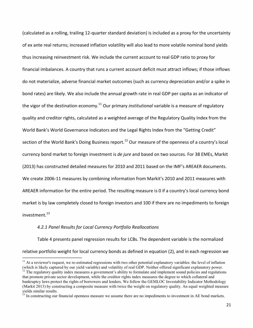
The evolution of bond markets is evident in the graphs in Figure 1. As a share of GDP, local
currency bond markets are largest in AEs, whereas EME bond markets are, on average, quite small
(Figure 1, top left). That said, the structure of many EME bond markets has improved dramatically over
6 Reduced reliance on foreign currency borrowing alleviated the fear of floating (Calvo and Reinhart 2002) and facilitated new policy regimes with inflation targeting central banks and flexible exchange rates. Improved policies and better developed local bond markets might have enabled EMEs in general, and Latin America in particular, to weather the global financial crisis much better than the Asian financial crisis of the late 1990s (Alvarez and De Gregorio 2013, Vegh and Vuletin 2013).
14
the past decade. Many EMEs have lessened their reliance on foreign currency bonds (Fig. 1, bottom
left). EME bond markets seem to have room to grow (that is, they are all small, as Fig. 1 top left shows),
and recent growth has been accompanied by a move toward an improved structure (that is, growth in
local currency bonds, with less of a dependence on foreign currency denominated debt).
Digging a bit deeper, we next split on the currency denomination of bonds issued by
governments vs. those issued by private entities. AE bonds (Fig. 1, top right) are mostly local currency
(blue bars for private; green bars for government). In EMEs (Fig. 1, bottom right), most bonds are
sovereign and denominated in the local currency (green bars), although local currency denominated
bonds issued by the private sector (blue bars) have increased sharply since 2007.
3.2 Historical Return Characteristics
We next describe characteristics of USD returns for various asset classes over the past decade
(Table 2).7 We first examine unhedged local currency EME bonds. Over the period January 2003–
October 2013 (Panel A), unhedged local currency EME bonds provided equity-like returns: strong mean
(0.91% per month), relatively high volatility (variance higher than other bonds but lower than equities),
and moderately negative skewness (in line with the skewness of equities). The high volatility of
unhedged EME local bonds is as expected. Currencies are more volatile than most assets, so the USD
returns on local currency EME bonds are also volatile. Correlations with US government bonds provide
one measure of potential diversification benefits; unhedged local currency EME bonds presented a
very low correlation (0.13) with US government bonds. Since the beginning of the global financial crisis
(the August 2007 to October 2013 period, shown in Panel B), the characteristics of unhedged EME local
7 The sample period for Table 2 is dictated by data availability. GBI-EM indices begin in December 2002, so January 2003 is the first monthly return. Our GBI dataset ends October 2013.
15
currency bonds have been similar to the full sample period: relatively high returns with elevated
volatility (but less volatile than equities), some negative skewness, and a low correlation with US
government bonds. This strong multi-year performance holds even though 2013, with its taper
tantrum, was the worst year for EME debt since at least 2003 (the first year EME local currency bond
indices were available).
EME returns hedged against currency changes—although we note that hedging in such markets
might be cost prohibitive for portfolio investors—show moderate returns that are not dissimilar from
the returns on US government bonds and in a sense lie somewhere between hedged and unhedged AE
bond returns.8
Turning to other asset classes, AE local currency bonds look very much like US bonds. Unhedged
AE bonds are more volatile than hedged AE bonds, not surprisingly, and over the two time periods
these provided higher returns (because the USD depreciated, adding to the returns that unhedged
foreign-currency denominated bonds provided US investors). Skewness is near zero for AE bonds,
whether hedged or unhedged. Dollar-denominated EME bond returns (EMBI) are relatively high, with
moderate volatility but very negative skewness. Over the entire period equity returns were highest in
EMEs, but with very high volatility; since August 2007 US equity markets have provided the highest
return. Notably, EME bond returns compare favorably—or are at least comparable—to US equities.
We caution that the return characteristics for EME bonds portrayed in Table 2 are likely more
favorable than those in previous periods, because the U.S. dollar depreciated against many currencies
over the past decade, adding to unhedged local currency bond returns translated into dollars. Were
the dollar to appreciate materially, unhedged EME bond returns would suffer. For example, in the
8 Large institutions, such as mutual funds, that invest in local currency EME bonds can hedge the currency risk using one- or two-month forward contracts, but for EME currencies hedge products with longer horizons are rare.

16
1990s, although systematic local currency EME bond returns were not available, previous estimates
(Burger and Warnock 2007) suggest returns were highly volatile (because inflation and exchange rates
were volatile) and negatively skewed (because spikes in bond yields and, hence, negative returns on
the underlying bonds coincided with financial flight that depreciated the currency). In AE bond
markets, at least prior to the eurozone debt crisis, periods of negative bond returns often coincided
with currency appreciation, eliminating the occasional extremely bad outcome for international
investors. In contrast, in EMEs, the bad outcome of negative bond returns was often exacerbated by a
plummeting currency. The good news for global fixed-income investors is that in the past decade the
improved stability achieved by a number of EMEs has been helpful in alleviating the combined bad
outcomes of losses on bonds and a depreciating currency (hence EME local currency bond returns are
not too negatively skewed).
Efficient frontiers reveal additional information about the January 2003–October 2013 returns.
Figure 2 (top graph) shows three all-bond efficient frontiers to illustrate risk–return trade-offs facing a
US-based fixed-income investor. Each frontier includes a range of bond portfolios, varying from 100%
U.S. bonds (the common point in each line) to 100% foreign bonds. The figure includes three measures
of the rest-of-world (ROW) portfolio: (1) an unhedged portfolio of 80% AE and 20% EME bonds, (2) a
hedged portfolio of 80% AE and 20% EME bonds, and (3) a 50/50 combination of (1) and (2).
The frontiers provide a few important lessons. First, the attractiveness of local currency bonds
for cross-border investors can be impeded by significant currency risk. From the perspective of a U.S.
investor, adding unhedged foreign bonds significantly increases portfolio risk. For the January 2003–
October 2013 period, the added risk happened to be compensated by strong returns (in part because
of the depreciating U.S. dollar), but in periods of an appreciating US dollar (not shown), the additional

17
risk could be accompanied by substantially lower returns. The figure also indicates the gains to
diversification from adding hedged foreign bonds, which over this period (and earlier periods) reduced
portfolio risk without much deterioration of returns. A mix of hedged and unhedged bonds provided a
particularly attractive risk–return trade-off over this period. This finding suggests that, although
choosing not to hedge the currency risk makes a cross-border investment in EME local currency bonds
largely a currency play (with some yield) in an instrument that might not be as liquid as desired, global
investors will likely prefer bonds in countries where they have the option to hedge the currency risk.
The bottom graph of Figure 2 broadens the set of assets to all those included in Table 2. We
selected weights for each asset class from 2006. Weights for the U.S. portion are based on 2006
estimates from the U.S. Federal Reserve’s flow of funds accounts: 62% equities and 38% bonds—of
which 43% are government bonds and 57% are corporate bonds. For the ROW portion, the weights—
which come from U.S. Treasury Department surveys—are 77% equities and 23% bonds; the equity
portion is 79% AE and 21% EME, and the bond portion is 89% AE, 9% USD-denominated EME, and 2%
local currency EME. As in the top panel, we allowed for bond portfolios being unhedged or hedged
against currency fluctuations, and the 100% US portfolio is the common point in each line. Over the
January 2003–October 2013 period, efficient frontiers for the broader portfolio are upward sloping;
more return was accompanied by more risk.
In summary, for a USD-based investor unhedged local currency EME bonds are largely a
currency play against the U.S. dollar (with some yield), so mean returns depend on how EME
currencies perform against the U.S. dollar. Hedged returns are more stable but offer somewhat smaller
diversification benefits. A combination of hedged and unhedged EME bonds has provided particularly
attractive return characteristics.

18
4 US Portfolios
4.1 Descriptive Analysis
Table 3 provides an end-2011 snapshot of US portfolios. Evolution through time is provided in
Figures 3 and 4. The local currency bond portfolio of US investors has grown from $152 billion in 2001
to almost $500 billion in 2011 (Figure 3, top panel). The foreign-issued USD-denominated portfolio is
substantially larger at almost $1500 billion; most of the USD-denominated foreign bonds were issued
by private sector entities in just a handful of countries such as Caribbean Financial Centers, Australia,
Canada, the Netherlands, and Sweden (Bertaut, Tabova, and Wong 2013).
Overall, local currency bonds have been a relatively stable 25-30 percent of US investors’
foreign bond portfolio. But for EMEs the story is quite different: the share of local currency bonds in US
investors’ EME bond portfolios has skyrocketed from about 2% in 2001 to almost 40% in 2011 (Figure
3, bottom panel). Gone are the days when US investors shunned local-currency denominated EME
bonds.
While most US holdings of local currency bonds are in AEs (Fig. 4.1, top left), US holdings of
EME LCBs have increased substantially over the past decade (Fig. 4.1, bottom left). With both the
amount invested and the size of the markets increasing, it is an open question whether US investors
have become less underweight in these markets. Interestingly, not only have US investors have
become less underweight in many EME LCBMs, they are less underweight in EMEs than in AEs (Figure
4.1, top right). The variation we attempt to understand is within-country changes in US relative
weights. For example, Fig. 4.1 (bottom right) shows variation in US relative weights for one set of
countries—LatAm EMEs—for local currency bonds. With our regressions we aim to understand why,
for example, US investors became less underweight (i.e. relative weight increased) on Mexico in 2011.

19
Digging further into the splits of US holdings by issuer type and currency denomination reveals
some interesting facts. The vast majority of US holdings of AE bonds are USD-denominated bonds
issued by private entities (Fig. 4.2, top left, maroon bars). US holdings of AE government bonds are
primarily denominated in local currency (green bars). US EME holdings (Fig. 4.2, bottom left) are more
diverse, with the only split avoided being private-sector issued local currency bonds (a sector that has
grown substantially the past few years). Holdings of sovereign local currency bonds (green) has
increased the most since 2007 and is now the largest component, but holdings of sovereign USD-
denominated bonds (orange) are also quite large. Also sizeable are holdings of EME private-sector
USD-denominated bonds—a potential area of concern due to possible currency mismatches. Note that
relative weights for USD bonds (Fig. 4.2, top and bottom right; Table 3, rightmost block) tend to be
much higher than for local currency bonds.9
In summary, the weight of EME local currency bonds in US investors’ bond portfolios has
increased relative to the share of EME local currency bonds in the global bond market. EME local
currency bonds were 4.9% of the global local currency bond market in 2001 and grew to 7.8% in 2011,
but US holdings increased even faster, increasing from 1.1% of the cross-border local currency bond
portfolio in 2001 to 17.2% by 2011. The relative weight measure for EME local currency bonds in US
investors’ portfolios, after a dramatic increase over the past decade, now exceeds the relative weight
of AE local currency markets. In other words, in US investors’ portfolios of EME local currency bonds
are closer to benchmark (ICAPM) weights than are AE local currency bonds.
9 This fact—that relative weights are higher for bonds issued in the investors’ currency—likely holds for other investor countries and means that datasets like the IMF’s CPIS that do not differentiate by currency denomination mix very different assets.
20
4.2. Empirical Analysis of US Investors’ Foreign Bond Portfolios
Over the past decade, US investors have increased their cross-border holdings of local currency
bonds, especially in EMEs. We will use a common framework to analyze the evolution US investors’
country-specific relative portfolio weights—that is, their portfolio weights relative to a global
benchmark (as described in Section 2.1)—in various types of foreign bonds. Because changes in relative
weight can be due to passive or active reallocations, we follow Ahmed et al (2014) and normalize (1) by
the home relative weight to isolate active reallocations:
mUS
USUS
mi
USilWgtnorm
.
,
.
, /Re
(2)
Our annual panel dataset of US investor relative portfolio weights includes 38 destination
countries over the period 2006-2011.10 For explanatory variables, we include country-specific “pull”
factors such as yield (to proxy for expected return), macroeconomic indicators (GDP growth rate,
volatility of inflation, and current account balance), institutional variables, and a proxy for the
openness of a country’s bond market to foreign investment. For global “push” factors we include the
volatility index VIX (which measures variation in expected volatility and risk appetite), the 10-year US
Treasury rate (to capture a “reach for yield”), and a measure of unconventional monetary policy (or
UMP, defined as changes in the size of Federal Reserve securities holdings scaled by nominal GDP).
The macroeconomic indicators included in our regressions represent factors that likely impact
the attractiveness of an economy as a destination for cross-border bond investment. Inflation volatility
10 The number of destination countries is limited not by the holdings data, but by data on the size and composition of bond markets and for explanatory variables.
21
(calculated as a rolling, trailing 12-quarter standard deviation) is included as a proxy for the uncertainty
of ex ante real returns; increased inflation volatility will also lead to more volatile nominal bond yields
thus increasing reinvestment risk. We include the current account to real GDP ratio to proxy for
financial imbalances. A country that runs a current account deficit must attract inflows; if those inflows
do not materialize, adverse financial market outcomes (such as currency depreciation and/or a spike in
bond rates) are likely. We also include the annual growth rate in real GDP per capita as an indicator of
the vigor of the destination economy.11 Our primary institutional variable is a measure of regulatory
quality and creditor rights, calculated as a weighted average of the Regulatory Quality Index from the
World Bank’s World Governance Indicators and the Legal Rights Index from the “Getting Credit”
section of the World Bank’s Doing Business report.12 Our measure of the openness of a country’s local
currency bond market to foreign investment is de jure and based on two sources. For 38 EMEs, Markit
(2013) has constructed detailed measures for 2010 and 2011 based on the IMF’s AREAER documents.
We create 2006-11 measures by combining information from Markit’s 2010 and 2011 measures with
AREAER information for the entire period. The resulting measure is 0 if a country’s local currency bond
market is by law completely closed to foreign investors and 100 if there are no impediments to foreign
investment.13
4.2.1 Panel Results for Local Currency Portfolio Reallocations
Table 4 presents panel regression results for LCBs. The dependent variable is the normalized
relative portfolio weight for local currency bonds as defined in equation (2), and in each regression we 11 At a reviewer's request, we re-estimated regressions with two other potential explanatory variables: the level of inflation (which is likely captured by our yield variable) and volatility of real GDP. Neither offered significant explanatory power. 12 The regulatory quality index measures a government’s ability to formulate and implement sound policies and regulations that promote private sector development, while the creditor rights index measures the degree to which collateral and bankruptcy laws protect the rights of borrowers and lenders. We follow the GEMLOC Investability Indicator Methodology (Markit 2013) by constructing a composite measure with twice the weight on regulatory quality. An equal weighted measure yields similar results. 13 In constructing our financial openness measure we assume there are no impediments to investment in AE bond markets.
22
include fixed destination-country effects and cluster standard errors by country. In the left half of the
table, in addition to the country fixed effects we also include time fixed effects (and thus must omit the
global “push” factors); in the right half we omit the time fixed effects and include specific global
factors. The time effects capture the impact of global forces on relative local currency bond allocations
during each year in the sample; coefficients for 2007-2011 are reported and should be interpreted
relative to 2006.
Results from the two-way fixed-effects specification for the full sample as well as the AE and
EME subsamples are reported in the first three columns of Table 4. Two things are striking: the model
has much greater explanatory power for EMEs (to a first approximation, US investors do not appear to
differentiate between AE local currency bond markets) and the time fixed effects suggest substantial
reallocations toward EME bond markets. Specifically, while none of the explanatory variables are
significant in the AE subsample (col. 2), for the EME subsample (col. 3) we find a significant impact for
local and global factors. The coefficients on the time dummies suggest a steady increase in allocations
toward local currency EME bonds over the time period, even during the height of the global financial
crisis. Local factors also mattered: US investors reallocated toward local currency bond markets of
EMEs with higher bond yields, faster economic growth, more positive current account balances and
more stable inflation. Our estimates indicate that the most economically significant local factor is
inflation volatility. For example, the coefficients in column (3) of Table 4 suggest that the stabilization
of South African inflation over our sample period explains roughly 25% of US investors’ reallocation
into rand-denominated bonds.
The advantage of the two-way fixed-effects specification is that it shows the impact of global
forces on bond allocations over time without having to specify the precise nature of the global

23
variables. The disadvantage is that all the global factors are rolled into one (the time dummies), which
does not allow specific interpretation of, for example, the roles of US monetary policy and global risk
aversion. Given the difficulty in properly capturing these specific global factors, one could argue that
the two-way fixed effects is the sounder econometric approach, but for completeness in columns 4-6
we omit the time fixed effects and include global “push” factors. Once again the model has much more
explanatory power for EMEs (col. 6) and we again find an important role for both global and country-
specific factors. When US Treasury rates fall, US investors increase positions in EME local currency
bond markets. The positive coefficient on the Federal Reserve’s Large Scale Asset Purchases (LSAP)
suggests a statistically significant “push” effect of UMP that is beyond the conventional channel of US
Treasury rates. In addition, US investors decrease their cross-border exposure to EME local currency
bonds during periods of increased volatility (and/or risk aversion). Local factors also matter in these
specifications. Local currency bond investors tended to reallocate away from volatile inflationary
environments and into economies with stronger economic growth rates. The coefficients on the
country-level institutional variables are statistically insignificant, but given the limited time variation in
these variables much of their explanatory power is likely absorbed by the country-level fixed effects.
In general, the results in Table 4 are consistent with the notion that UMP pushed US investors
into EME bonds during this time period, but local factors mattered too. To gauge the relative
importance of global and local factors we follow Bekaert and Wang (2009) and conduct a variance
decomposition (VARC) analysis. The relative explanatory power of regressor X is computed as:
)ˆvar(),ˆcov(ˆ
y
xyVARC xx (3)
By construction the VARCs of all the regressors sum to one, therefore the VARC for a particular
explanatory variable represents its relative contribution. Focusing on EMEs, for the model in column

24
(3) we find that 42% of the variation is determined by our local explanatory variables while 58% of the
variation is explained by global factors.14 Of the local variables inflation volatility has the highest VARC
at 23%. Repeating the exercise for column (6) produces essentially the same split between local and
global factors, with the US 10-yr Treasury rate dominating with a VARC of 51%. That is, the classic
result of low US rates being associated with a surge in EME investment holds when we focus on EME
local currency bonds, providing a plausible channel through which US monetary policy could have
contributed to the appreciation of EME currencies (and thus provides support to currency war claims).
4.2.2 Panel Results on USD-denominated Portfolio Reallocations
While our primary focus is on local currency bonds, in Table 5 we analyze portfolio reallocations
in USD-denominated bonds. The dependent variable for our empirical analysis of USD-denominated
bonds is normalized relative weight, where relative weight is defined as:
i
iusdiusd
i
US
iusd
US
iusd
mi
USi
MCapMCap
HH
/.
,
(4)
where US
iusd H is US investors’ holdings of country i’s USD-denominated bonds and i
US
iusd H
represents the global portfolio of USD-denominated bonds held by US investors, while iusd MCap is the
market capitalization of country i’s USD-denominated bond market and i
iusd MCap is the market
capitalization of the global USD-denominated bond market. Once again we include fixed destination-
country effects, either time fixed effects or global “push” factors, and country-level “pull” factors.
In contrast to the results for local currency bonds, the time fixed effects in Table 5 are almost
always insignificant; any broad reallocation toward USD-denominated bonds only occurred for EMEs
14 Note that we are decomposing the variance net of the country fixed effects.
25
and only at the very end of our sample (and even then the time dummy is only marginally significant).
The reallocation toward USD-denominated EME bonds is associated with lower US rates and lower VIX
(col. 6). Although most time effects are statistically insignificant, it is notable that we find a negative
and marginally statistically significant coefficient for EMEs in 2008. In other words, in contrast to our
results for local currency bonds, here we find some (weak) evidence that US investors reduced their
cross-border holdings of USD-denominated EME bonds during the global financial crisis.
While the effects of global factors are muted in Table 5, we do find a significant impact of local
factors on US investment in USD-denominated EME bonds. The results in columns (3) and (6) indicate
that more positive current account balances and lower inflation volatility were also associated with
rising relative US allocations. To gauge the relative importance of global and local factors we again
conduct a variance decomposition analysis, this time for the USD-denominated allocations of columns
(3) and (6). For the time effects specification we find that 78% of the variance is explained by local
factors, with the most important variables being current account (59%) and inflation volatility (17%).
Repeating the exercise with specific global factors reveals a similar local-global split—local factors
matter most for reallocations within the USD-denominated EME bond portfolio—with the most
important global factor being VIX (17%).
4.2.3 Sectoral Results
Tables 6 and 7 show results split by the sector (private or government) that issued the bond.15
For local currency (Table 6) or USD-denominated bonds (Table 7), the sectoral results show that our
main regressions are most able to explain portfolio reallocations within government bond portfolios.
Results for the government bonds columns in Tables 6 and 7 are quite similar to those in Tables 4 and
15 Sectoral splits for US holdings are available beginning in 2007, therefore reducing the sample size relative to the results reported in Tables 4 and 5.

26
5. The time effects in columns (2) and (3) of Table 6 indicate a reallocation away from AE sovereign
bond markets and into EME sovereign bonds throughout the sample period. For samples restricted to
private-sector bonds, there is very limited explanatory power and very few significant coefficients,
although in Table 7 we do find negative coefficients on the time effects (statistically significant for 2011
and marginal for earlier years) for USD-denominated private sector bonds issued by AEs.
5. Conclusion
In 2007 when market volatility was on the rise (but nowhere near its peak), the Bundesbank
pondered (see opening quote) the role emerging LCBMs would play in promoting (or inhibiting) global
financial stability. The ensuing global financial crisis provided a severe test for these newly developed
markets, EMEs avoided another round of currency crises and US investors did not blindly flee the newly
developed asset class. Our data indicate that, on average, US investors increased their EME local
currency bond allocations during the crisis and this reallocation toward local currency EME bonds
accelerated in the post-crisis period. Moreover, our evidence suggests that US investors do not treat
EME local currency bonds as a homogenous asset class, but rather discriminate among EMEs based on
macroeconomic fundamentals including inflation volatility, current account balances, and real GDP
growth rates.
Overall, our results have interesting implications for financial stability and help distinguish
between the possibilities of virtuous and vicious cycles in local currency bond markets. The importance
of global monetary conditions and risk appetite/expected volatility lend credence to the concerns of
EME policy makers who worry that volatile flows will influence exchange rates and real activity. Fears
of a vicious cycle with indiscriminate herd-like flows into and out of EMEs are quelled somewhat by our

27
finding that US investors’ discriminate among EMEs based on macroeconomic fundamentals. Strong
macroeconomic conditions should help EMEs attract and retain cross-border investment, which would
reinforce a more virtuous cycle in local currency bond markets.

28
References
Ahmed, S., S. Curcuru, F. Warnock, and A. Zlate, 2014. The Many Forms of International Capital Flows.
mimeo.
Alvarez, R. and J. De Gregorio, 2013. “Why did Latin America and Developing Countries Perform Better
in the Global Financial Crisis than in the Asian Crisis?” working paper presented to IMF’s 14th
Annual Research Conference.
Ammer, J., S. Holland, D. Smith, and F. Warnock, 2012. US International Equity Investment. Journal of
Accounting Research 50(5): 1109-1139.
Asian Development Bank, 2013. Broadening the investor base for local currency bonds in ASEA+2
countries.
Bekaert, G., and X. Wang, 2009, Home bias revisited, unpublished working paper.
Bertaut, C., A. Tabova, and V. Wong, 2013. “The replacement of safe assets in the US financial bond
portfolio and implications for the US financial bond home bias,” Working Paper, Federal Reserve
Board.
Blank, S., and C. Buch, 2007. The Euro and Cross-Border Banking: Evidence from Bilateral Data.
Comparative Economic Studies 49: 389-410.
Burger, J., and F. Warnock, 2003. “Diversification, Original Sin, and International Bond Portfolios,”
International Finance Discussion Paper #755, Board of Governors of the Federal Reserve System.
Burger, J., and F. Warnock, 2006. “Local Currency Bond Markets,” IMF Staff Papers 53: 133-146.
Burger, J., and F. Warnock, 2007. “Foreign Participation in Local-Currency Bond Markets,” Review of
Financial Economics 16(3): 291-304.
Burger, J., F. Warnock, and V. Warnock, 2012. “Emerging Local Currency Bond Markets,” Financial
Analysts Journal 68(4):73-93.
Calvo, Guillermo, Leonardo Leiderman, and Carmen Reinhart. (1993). “Capital Inflows and Real
Exchange Rate Appreciation in Latin America: The Role of External Factors.” IMF Staff Papers 40(1):
108–151.
Calvo, G. and C. Reinhart, 2002. “Fear of Floating,” Quarterly Journal of Economics 177: 379-408.
Chuhan, Punam, Stijn Claessens, and Nlandu Mamingi. (1998). “Equity and bond flows to Latin America
and Asia: The Role of Global and Country Factors.” Journal of Development Economics 55 (2), 439 -
463.
Claessens, S., D. Klingebiel, and S. Schmukler, 2007. “Government Bonds in Domestic and Foreign
Currency: The Role of Institutional and Macroeconomic Factors.” Review of International Economics
15(2): 370-413.
Cooper, I., and E. Kaplanis, 1986. Costs to crossborder investment and international equity market
equilibrium. in J. Edwards, J. Franks, C. Mayer and S. Schaefer (eds.), Recent Developments in
Corporate Finance. Cambridge University Press, Cambridge.

29
Eichengreen, B., and R. Hausmann, 1999. Exchange rates and financial fragility. Proceedings, Federal
Reserve Bank of Kansas City, pages 329-368.
Eichengreen, B. and P. Luengnaruemitchai, 2006. “Why Doesn’t Asia Have Bigger Bond Markets?” In
BIS Papers No 30: Asian Bond Markets: Issues and Prospects. Basel, Switzerland: Bank for
International Settlements.
Felettigh, A., and P. Monti, 2008. How to interpret the CPIS data on the distribution of foreign portfolio
assets in the presence of sizeable cross-border positions in mutual funds. Evidence for Italy and the
main euro-area countries. Banca d’Italia Occasional Paper No. 16.
Fidora, M., M. Fratzscher, and C. Thimann, 2007. Home Bias in Global Bond and Equity Markets: The
Role of Real Exchange Rate Volatility. Journal of International Money and Finance 26: 631-655.
Fratzscher, M., 2012. “Capital Flows, Push Versus Pull Factors and the Global Financial Crisis,” Journal
of International Economics 88(2): 341-356.
Forbes, K., and F. Warnock, 2013. “Debt- and Equity-Led Capital Flow Episodes,” in Capital Mobility and
Monetary Policy edited by Miguel Fuentes and Carmen M. Reinhart. Santiago: Central Bank of
Chile. Also available as NBER Working Paper No. 18329.
Goldstein, M., and P. Turner, 2004. Controlling Currency Mismatches in Emerging Economies.
Washington, DC: Institute for International Economics.
Gourinchas, P.‐O., and M. Obstfeld, 2012. “Stories of the Twentieth Century for the Twenty‐First,”
American Economic Journal: Macroeconomics 4(1): 226‐65.
Griever, W., G. Lee, and F. Warnock, 2001. The U.S. system for measuring cross-border investment in
securities: a primer with a discussion of recent developments. Federal Reserve Bulletin 87(10): 633-
650.
Gruić, B., and P. Wooldridge, 2012. Enhancements to the BIS debt securities statistics. BIS Quarterly
Review (December, pages 63-76).
Hale, G., and M. Obstfeld, 2014. The Euro and the Geography of International Debt Flows. mimeo.
Holland, S., S. Sarkissian, M. Schill, and F. Warnock, 2013. Global cross-border equity holdings. Mimeo.
J.P. Morgan, 2002. JPMorgan Government Bond Indices. J.P. Morgan Portfolio Research, January 14.
J.P. Morgan, 2006. Introducing the JPMorgan Government Bond Index-Emerging Markets (GBI-EM):
Index Methodology. J.P. Morgan Emerging Markets Research and Bond Index Research, January.
Lane, P., 2006. Global Bond Portfolios and EMU. International Journal of Central Banking 2(2): 1-23.
Markit Indices Limited, 2013. “GEMLOC Investability Indicator Methodlogy,” February 2013,
https://www.markit.com/assets/en/docs/products/data/indices/bond-
indices/GEMLOC%20Investability%20Indicator%20Methodology.pdf
McCauley, R., C. Upper, and A. Villar, 2013. Emerging market debt securities issuance in offshore
centers. BIS Quarterly Review (September, Box 2).
Mendoza, E. and M. Terrones, 2008. “An Anatomy of Credit Booms: Evidence from Macro Aggregates
And Micro Data,” NBER Working Paper No. 14049.

30
Milesi-Ferretti, G.M., and C. Tille, 2012. The great retrenchment: international capital flows during the
global financial crisis. Economic Policy 26(66): 289-346.
Moore, J., S. Nam, M. Suh, and A. Tepper, 2013. Estimating the Impacts of U.S. LSAPs on Emerging
Market Economies’ Local Currency Bond Markets. Federal Reserve Bank of New York Staff Reports,
no. 595.
Raddatz, C., S.Schmukler, 2012. “On the international transmission of shocks: Micro-evidence from mutual fund portfolios,” Journal of International Economics 88(2): 357-374.
Schularick, M., and A. M. Taylor, 2012. “Credit Booms Gone Bust: Monetary Policy, Leverage Cycles, and Financial Crises, 1870‐2008.” American Economic Review 102: 1029‐61.
Tille, Cedric, and Eric van Wincoop, 2010. International Capital Flows. Journal of International Economics 80(2): 157-175.
U.S. Department of the Treasury, Federal Reserve Bank of New York, and Board of Governors of the Federal Reserve System, 2002. Report on Foreign Portfolio Investment in the United States as of December 31, 2001.
________ 2007. Report on Foreign Portfolio Investment in the United States as of December 31, 2006. ________ 2009. Report on Foreign Portfolio Investment in the United States as of December 31, 2008. ________ 2012. Report on Foreign Portfolio Investment in the United States as of December 31, 2011. Vegh, C. and G. Vuletin, 2013. “The Road to Redeption: Policy Response to Crises in Latin America,”
working paper presented to IMF’s 14th Annual Research Conference.

31
Data Appendix
Throughout, “bonds” refer to debt instruments with greater than one year original maturity. We focus on bonds denominated in the currency of the country in which the issuer resides. Bond Returns
Our main source of returns data is country-level JPMorgan Government Bond Indexes (GBI) and JPMorgan Government Bond Indexes-Emerging Markets (GBI-EM). See J.P. Morgan (2002, 2006) for complete descriptions.
GBI consists of “regularly traded, fixed-rate, domestic government bonds of countries that offer opportunity to international investors. These countries have liquid government debt markets, which are stable, actively traded markets with sufficient scale, regular issuance and are freely accessible to foreign investors.” The indices should be representative (span and weight the appropriate markets, instruments and issues that reflect opportunities available to international investors) and investible and replicable (include only securities in which an investor can deal at short notice and for which firm prices exist). The 13 countries in the original GBI include Australia, Belgium, Canada, Denmark, France, Germany, Italy, Japan, Netherlands, Spain, Sweden, UK, and the US.
The GBI-EM is similar to the main GBI in methodology but tracks emerging markets economies. Some of the bonds are speculative; some EM bond markets are not directly hedgeable. Countries in the GBI-EM include Brazil, Chile, Colombia, Czech Republic, Hungary, Indonesia, Malaysia, Mexico, Poland, Slovakia, South Africa, Thailand, and Turkey. Bonds in the countries in the narrow GBI-EM should be easy to access, with no impediments for foreign investors. A few countries with sizeable local bond markets but that have substantial restrictions on foreigners (China, India, Russia) are added to create the GBI-EM BROAD, which has 16 EMEs.
JPMorgan returns data are available for positions that are unhedged and hedged using exchange rates and forward rates from WM Company as of 4pm London time. Hedging for a few countries in the GBI-EM has not always been possible (e.g., Malaysia, Chile), so hedged returns for some EMs should be viewed as indicative but not actual. Please see Appendix E of JPMorgan (2006) for complete details.
We also include for comparison a US corporate bond index, a dollar-denominated EME bond index (JPMorgan’s EMBI), and three equity indices. The Dow Jones Corporate Bond Index is an equally weighted basket of 96 recently issued, readily tradable, investment-grade corporate bonds. We use the index with 5-year maturity. The equity indices are the S&P500 (for the US), MSCI EM, and MSCI EAFE+Canada; see www.msci.com/products/indices/tools/index.html for details on the MSCI data. Bonds Outstanding We use two complementary sources of data on the amount of a country’s outstanding local currency bonds. Both are from the Bank for International Settlements (BIS), which compiles data from multiple sources. Note that BIS changed methodology in 2012 (see Gruić and Wooldridge 2012) and the newer data might not be consistent with the historical data, so our analysis ends in 2011 and our description refers to the pre-2012 BIS methodology.
One data set is on “domestic debt”, which the BIS defines as local currency bonds issued by locals in the local market (i.e., not placed directly abroad). Data are available in BIS Quarterly Review Table 16A (Domestic Debt Securities). Because our focus is on bonds (with original maturity longer than one year), we obtained the data underlying Table 16A to separate short term from long term.
The other data set is on “international bonds”, bonds issued either in a different currency or in a different market. Certain aggregates of this are presented BIS Quarterly Review Table 14B (International Bonds and Notes by Country of Residence). For our focus we obtained the underlying data, as issuance by currency by country is not presented in the Quarterly Review.
With these two sources (and our calculations), local-currency-denominated debt is the sum of the long-term debt component of “domestic debt” and the local currency / local issuer portion of “international bonds”. USD-denominated debt is the USD portion of “international bonds”. Our measure includes all bonds issued by all types of issuers (government and private).

32
US Bond Holdings
Data on US investors’ holdings of local currency bonds is from periodic, comprehensive benchmark surveys conducted by the Treasury Department, Board of Governors of the Federal Reserve System, and the Federal Reserve Bank of New York. See the actual surveys, for example, Treasury Department et al. (2002, 2009) or the Griever, Lee, and Warnock (2001) primer for details. Briefly, from Griever, Lee, and Warnock (2001), the so-called “asset surveys” of US holdings of foreign securities collect data from two types of reporters: US-resident custodians and US institutional investors. Custodians are the primary source of information, typically reporting about 97 percent of total US holdings of foreign long-term securities. Institutional investors, such as mutual funds, pension funds, insurance companies, endowments, and foundations, report in detail on their ownership of foreign securities only if they do not entrust the safekeeping of these securities to US-resident custodians. If they do use US-resident custodians, institutional investors report only the name(s) of the custodian(s) and the amount(s) entrusted (and the data are collected from the custodian, but not double counted).
Reporting on the asset surveys is mandatory, with both fines and imprisonment possible for willful failure to report. The data are collected at the security-level, greatly reducing reporting error; armed with a security identifier, a mapping to the currency of the bond and the residence of its issuer is straightforward. Reporting and the data are comprehensive, and the holdings data form the official US data on international positions (for example, the number for international bonds in the Bureau of Economic Analysis’s International Investment Position report is formed by aggregating the survey’s security-level information).
For our purposes, we needed a split (US holdings of local currency foreign bonds) not usually published in the Treasury Department reports, and so persuaded Treasury to include an ‘own currency’ column in the published table on holdings by country by currency (see, for example, Table A.6 of Treasury Department et al. 2009). This is our measure of US holdings of local currency bonds.
Other Variables
As explanatory variables in Tables 4-7, we use various data series. Yield is the yield-to-maturity in the GBI indexes from J.P Morgan and enters our regressions as an annual average. See J.P Morgan (2006) Appendix B. A number of other explanatory variables are from the IMF’s IFS database (inflation volatility is computed from three years of quarterly CPI inflation), WEO (current account balance is as a percent of GDP) or WDI (GDP growth, calculated as year-over-year growth in real GDP per capita). VIX and USi10 come from the St. Louis Federal Reserve Database (FRED) and are year-end observations of the CBOE volatility index and 10-year US Constant Maturity Treasury rate, respectively. Federal Reserve holdings of US bonds, used to create our LSAP variable, are from the Fed’s H.4.1 release. regcr is calculated as a weighted average of the Regulatory Quality Index from the World Bank’s World Governance Indicators and the Legal Rights Index from the “Getting Credit” section of the World Bank’s Doing Business report. The regulatory quality index measures a government’s ability to formulate and implement sound policies and regulations that promote private sector development, while the creditor rights index measures the degree to which collateral and bankruptcy laws protect the rights of borrowers and lenders. We follow the GEMLOC Investability Indicator Methodology (Markit 2013) by constructing a composite measure with twice the weight on regulatory quality. An equal weighted measure yields similar results. Finally, caopen is our measure of the openness of a country’s local currency bond market to foreign investment is de jure and based on two sources. For 38 EMEs, Markit (2013) has constructed detailed measures for 2010 and 2011 based on the IMF’s AREAER documents. We create our 2006-11 measures by combining information from Markit’s 2010 and 2011 measures with AREAER information for the entire period. The resulting measure is 0 if a country’s local currency bond market is by law completely closed to foreign investors and 100 if there are no impediments to foreign investment. In constructing our financial openness measure we assume there are no impediments to investment in AE bond markets. Country Groupings
The groupings of “advanced economies”, or AEs, and “other emerging market and developing countries” (shortened here to emerging market economies or EMEs) follow IMF classification as of April 2013. See http://www.imf.org/external/pubs/ft/weo/2013/01/pdf/statappx.pdf.
33
Figure 1. The Structure of Global Bond Markets
010
,000
20,0
0030
,000
40,0
00A
mou
nt O
utst
andi
ng ($
Billi
ons)
2006 2007 2008 2009 2010 2011
AE Bonds: LC and USD
AE Private LC AE Private USD (ex-US)AE Gov't LC AE Gov't USD (ex-US)
01,
000
2,00
03,
000
4,00
0A
mou
nt O
utst
andi
ng ($
Billi
ons)
2007 2008 2009 2010 2011
EM Bonds: LC and USD
EME Private LC EME Private USDEME Gov't LC EME Gov't USD

34
Figure 2. Efficient Frontiers for Bond Portfolios Returns data are from January 2003 to October 2013. Vertical axes are monthly returns (in percent); horizontal axes are standard deviation of the monthly returns. In the top graph, each frontier includes a range of portfolios varying from 100% U.S. bonds (the common point in each line) to 100% foreign bonds. The figure includes three definitions for the rest-of-world (ROW) portfolio: (1) an unhedged portfolio of 80 percent AE and 20 percent EME bonds (the upward-sloping blue line), (2) a hedged portfolio of 80 percent AE and 20 percent EME bonds (the downward-sloping red line), and (3) a 50-50 combination of (1) and (2) (the line in the middle). The bottom graph includes equities as well, with each frontier including a range of portfolios varying from 100% U.S. (the common point in each line) to 100% foreign. Weights for the U.S. portion are 2006 estimates from the Federal Reserve’s Flow of Funds accounts: 62% equities, 38% bonds, of which 43% government and 57% corporate. For the rest-of-world (ROW) portion, weights are from Treasury Department surveys: 77% equity (of which 79% AE and 21% EME) and 23% bond (89% AE, 9% USD-denominated EME, 2% local currency EME). While the frontiers are not distinguishable from one another, the figure does include three definitions for the ROW bond portfolio: (1) unhedged (blue line), (2) hedged (the red line), and (3) a 50-50 combination of (1) and (2) (the line in the middle).
.75
.8.8
5.9
.95
1
Mon
thly
Re
turn
(%
)
3.5 4 4.5 5 5.5Standard Deviation
Portfolio 1- equity & unhedged bond (2003-2013)
Portfolio 2- equity & hedged bond (2003-2013)
50% portfolio 1 and 50% portfolio 2
Efficient Frontiers (January 2003 - October 2013)

35
Figure 3. US Investors’ Foreign Bond Holdings by Currency, 2001-2011 The top panel shows, for end of year 2001 and 2006-11, the total amount (in billions of USD) of US investors’ foreign bond holdings (“Total”) as well as the amounts held in USD-denominated (“USD”) and local currency (“Local currency”) bonds. The bottom panel shows, for US investors’ foreign bond holdings as of year ends 2001 and 2006-11, the shares of AE and EME holdings that are denominated in the local currency.
0
500
1000
1500
2000
2500
2001 2006 2007 2008 2009 2010 2011
Total
USD
Local Currency
0
0.05
0.1
0.15
0.2
0.25
0.3
0.35
0.4
0.45
2001 2006 2007 2008 2009 2010 2011
Share of AE holdings in Local Currency
Share of EME holdings in Local Currency
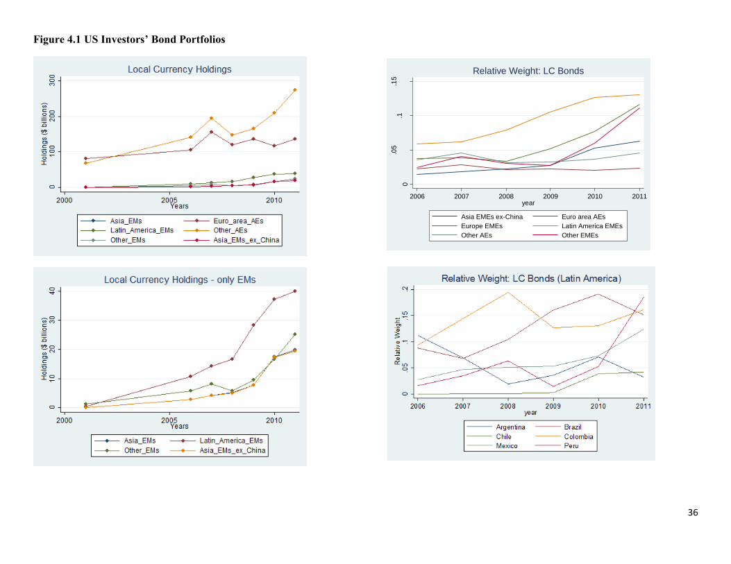
36
Figure 4.1 US Investors’ Bond Portfolios
0
.05
.1.1
5
Re
lative W
eig
ht
2006 2007 2008 2009 2010 2011year
Asia EMEs ex-China Euro area AEs
Europe EMEs Latin America EMEs
Other AEs Other EMEs
Relative Weight: LC Bonds

37
Figure 4.2 US Investors’ Bond Portfolios (continued)
0
20
040
060
080
0
Ho
ldin
gs (
$ B
illio
ns)
2007 2008 2009 2010 2011
AE Holdings: Pvt Govt LC USD
AE Private LC AE Private USD
AE Gov't LC AE Gov't USD
020
40
60
80
Ho
ldin
gs (
$ B
illio
ns)
2007 2008 2009 2010 2011
EME Holdings: Pvt Govt LC USD
EME Private LC EME Private USD
EME Gov't LC EME Gov't USD
.1.2
.3.4
.5.6
Re
lative W
eig
ht
2006 2007 2008 2009 2010 2011year
Asia EMEs Euro area AEs
Europe EMEs Latin America EMEs
Other AEs Other EMEs
Relative Weight: USD Bonds
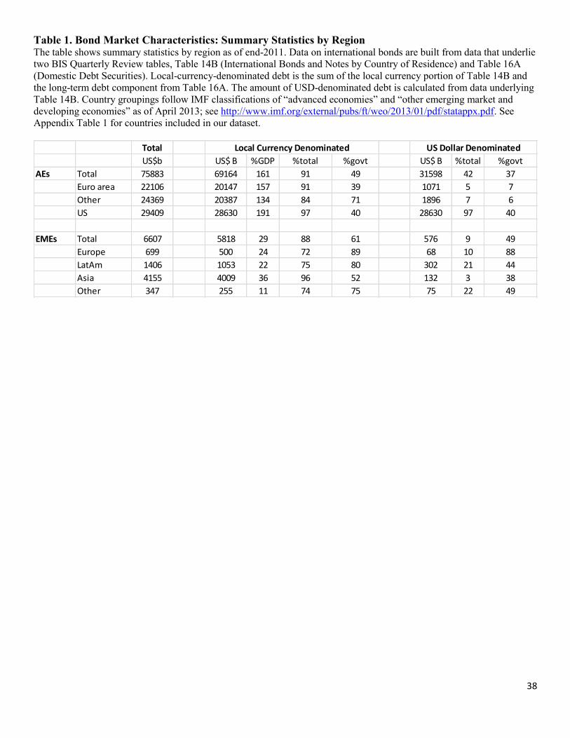
38
Table 1. Bond Market Characteristics: Summary Statistics by Region The table shows summary statistics by region as of end-2011. Data on international bonds are built from data that underlie two BIS Quarterly Review tables, Table 14B (International Bonds and Notes by Country of Residence) and Table 16A (Domestic Debt Securities). Local-currency-denominated debt is the sum of the local currency portion of Table 14B and the long-term debt component from Table 16A. The amount of USD-denominated debt is calculated from data underlying Table 14B. Country groupings follow IMF classifications of “advanced economies” and “other emerging market and developing economies” as of April 2013; see http://www.imf.org/external/pubs/ft/weo/2013/01/pdf/statappx.pdf. See Appendix Table 1 for countries included in our dataset.
Total
US$b US$ B %GDP %total %govt US$ B %total %govt
AEs Total 75883 69164 161 91 49 31598 42 37
Euro area 22106 20147 157 91 39 1071 5 7
Other 24369 20387 134 84 71 1896 7 6
US 29409 28630 191 97 40 28630 97 40
EMEs Total 6607 5818 29 88 61 576 9 49
Europe 699 500 24 72 89 68 10 88
LatAm 1406 1053 22 75 80 302 21 44
Asia 4155 4009 36 96 52 132 3 38
Other 347 255 11 74 75 75 22 49
Local Currency Denominated US Dollar Denominated

39
Table 2. Monthly U.S. Dollar Returns, January 2003–October 2013 The table shows return characteristics of various asset classes. AEs and EMEs consist of countries included in the J.P. Morgan GBI (excluding the United States) and GBI-EM Broad, respectively. EMBI is an index of USD-denominated EME bonds.
Mean Correlation with
(%) Variance Skewness US Govt Bonds
A. January 2003 to October 2013
EME local currency bonds
Unhedged 0.91 12.03 -0.85 0.13
Hedged 0.47 1.77 0.24 0.41
AE local currency bonds
Unhedged 0.49 5.78 0.02 0.55
Hedged 0.35 0.60 -0.10 0.77
Other Bonds
EMBI 0.84 6.72 -2.46 0.29
US Govt Bonds 0.37 1.99 -0.08 1.00
US Corp Bonds 0.55 3.39 -0.02 0.59
Equities
US 0.82 17.52 -0.83 -0.24
AE (ex US) 0.98 27.18 -0.87 -0.20
EMEs 1.46 46.19 -0.73 -0.18
B. August 2007 to October 2013
EME local currency bonds
Unhedged 0.69 16.89 -0.73 0.07
Hedged 0.42 2.50 0.40 0.41
AE local currency bonds
Unhedged 0.48 6.37 -0.15 0.54
Hedged 0.38 0.68 -0.14 0.76
Other Bonds
EMBI 0.73 8.85 -2.65 0.17
US Govt Bonds 0.43 2.06 0.44 1.00
US Corp Bonds 0.66 3.99 0.13 0.40
Equities
US 0.57 25.93 -0.71 -0.30
AE (ex US) 0.27 39.59 -0.60 -0.26
EMEs 0.44 61.65 -0.46 -0.25

40
Table 3. US Portfolios: Summary Statistics by Region The table shows summary statistics by region of US investors’ local currency and USD-denominated bond portfolios as of end-2011. Data are author’s calculations using data on US investment from the US Department of the Treasury et al. (2012) and the size of local currency bond markets (mostly from the BIS; see Table 1 for details). Relative weight measures, defined in the text equation (1), are calculated as the the weight of the country in US portfolios relative to its weight in the world market portfolios. A relative weight measure equals one if the weight of the countries’ bonds in US and world market portfolios are identical and is less than one if US investors’ underweight the country (relative to its market size). See Appendix Table 2 for country-level detail on local currency bond portfolios.
Total
US$b US$ B Relwgt GovtRelWgt PvtRelWgt US$ B Relwgt GovtRelWgt PvtRelWgt
AEs Total(ex-us) 1140 409 0.04 0.08 0.02 894 0.44 0.58 0.39
Euro area 374 136 0.03 0.07 0.01 230 0.32 0.14 0.29
Other 961 273 0.05 0.08 0.03 664 0.51 0.87 0.44
EMEs Total 226 85 0.06 0.13 0.004 133 0.31 0.46 0.23
Europe 37 17 0.13 0.22 0.01 14 0.30 0.42 0.14
LatAm 130 40 0.14 0.26 0.03 88 0.36 0.46 0.33
Asia 37 20 0.02 0.05 0.001 17 0.20 0.40 0.11
Local Currency Denominated US Dollar Denominated
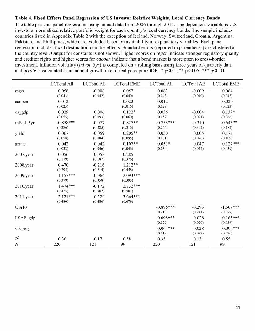
41
Table 4. Fixed Effects Panel Regression of US Investor Relative Weights, Local Currency Bonds The table presents panel regressions using annual data from 2006 through 2011. The dependent variable is U.S investors’ normalized relative portfolio weight for each country’s local currency bonds. The sample includes countries listed in Appendix Table 2 with the exception of Iceland, Norway, Switzerland, Croatia, Argentina, Pakistan, and Phillipines, which are excluded based on availability of explanatory variables. Each panel regression includes fixed destination-country effects. Standard errors (reported in parentheses) are clustered at the country level. Output for constants is not shown. Higher scores on regcr indicate stronger regulatory quality and creditor rights and higher scores for caopen indicate that a bond market is more open to cross-border investment. Inflation volatility (infvol_3yr) is computed on a rolling basis using three years of quarterly data and grrate is calculated as an annual growth rate of real percapita GDP. * p<0.1; ** p<0.05; *** p<0.01 LCTotal All LCTotal AE LCTotal EME LCTotal All LCTotal AE LCTotal EME regcr 0.058 -0.008 0.057 0.063 -0.009 0.064 (0.043) (0.042) (0.040) (0.043) (0.040) (0.043) caopen -0.012 -0.022 -0.012 -0.020 (0.025) (0.016) (0.029) (0.023) ca_gdp 0.029 0.006 0.122* 0.036 -0.004 0.139* (0.055) (0.093) (0.060) (0.057) (0.091) (0.066) infvol_3yr -0.858*** -0.077 -0.827** -0.758*** -0.310 -0.645** (0.286) (0.285) (0.316) (0.244) (0.302) (0.282) yield 0.067 -0.059 0.205** 0.050 0.005 0.174 (0.058) (0.084) (0.095) (0.061) (0.076) (0.109) grrate 0.042 0.042 0.107** 0.053* 0.047 0.127*** (0.032) (0.046) (0.046) (0.030) (0.047) (0.039) 2007.year 0.056 0.053 0.285 (0.179) (0.187) (0.376) 2008.year 0.470 -0.216 1.212** (0.295) (0.214) (0.458) 2009.year 1.157*** -0.064 2.093*** (0.379) (0.358) (0.395) 2010.year 1.474*** -0.172 2.732*** (0.425) (0.302) (0.507) 2011.year 2.121*** 0.524 3.664*** (0.480) (0.486) (0.679) USi10 -0.896*** -0.295 -1.507*** (0.210) (0.241) (0.277) LSAP_gdp 0.098*** 0.028 0.165*** (0.029) (0.029) (0.036) vix_eoy -0.064*** -0.028 -0.096*** (0.018) (0.022) (0.026) R
2 0.36 0.17 0.58 0.35 0.13 0.55 N 220 121 99 220 121 99
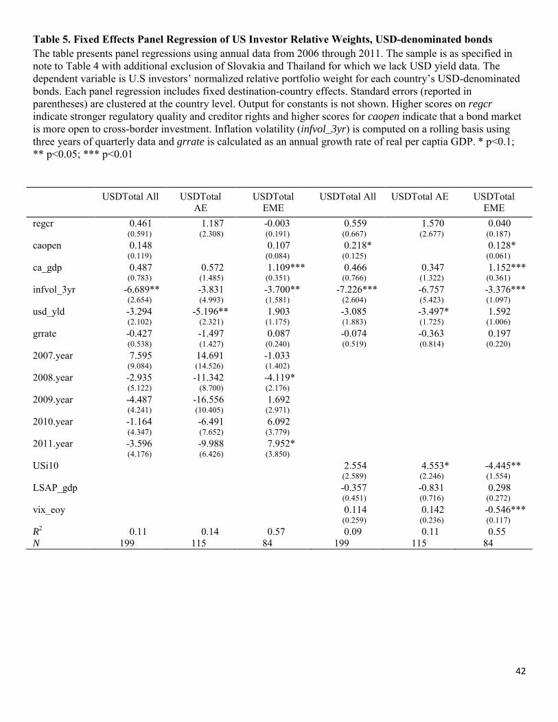
42
Table 5. Fixed Effects Panel Regression of US Investor Relative Weights, USD-denominated bonds The table presents panel regressions using annual data from 2006 through 2011. The sample is as specified in note to Table 4 with additional exclusion of Slovakia and Thailand for which we lack USD yield data. The dependent variable is U.S investors’ normalized relative portfolio weight for each country’s USD-denominated bonds. Each panel regression includes fixed destination-country effects. Standard errors (reported in parentheses) are clustered at the country level. Output for constants is not shown. Higher scores on regcr indicate stronger regulatory quality and creditor rights and higher scores for caopen indicate that a bond market is more open to cross-border investment. Inflation volatility (infvol_3yr) is computed on a rolling basis using three years of quarterly data and grrate is calculated as an annual growth rate of real per captia GDP. * p<0.1; ** p<0.05; *** p<0.01
USDTotal All USDTotal AE
USDTotal EME
USDTotal All USDTotal AE USDTotal EME
regcr 0.461 1.187 -0.003 0.559 1.570 0.040 (0.591) (2.308) (0.191) (0.667) (2.677) (0.187) caopen 0.148 0.107 0.218* 0.128* (0.119) (0.084) (0.125) (0.061) ca_gdp 0.487 0.572 1.109*** 0.466 0.347 1.152*** (0.783) (1.485) (0.351) (0.766) (1.322) (0.361) infvol_3yr -6.689** -3.831 -3.700** -7.226*** -6.757 -3.376*** (2.654) (4.993) (1.581) (2.604) (5.423) (1.097) usd_yld -3.294 -5.196** 1.903 -3.085 -3.497* 1.592 (2.102) (2.321) (1.175) (1.883) (1.725) (1.006) grrate -0.427 -1.497 0.087 -0.074 -0.363 0.197 (0.538) (1.427) (0.240) (0.519) (0.814) (0.220) 2007.year 7.595 14.691 -1.033 (9.084) (14.526) (1.402) 2008.year -2.935 -11.342 -4.119* (5.122) (8.700) (2.176) 2009.year -4.487 -16.556 1.692 (4.241) (10.405) (2.971) 2010.year -1.164 -6.491 6.092 (4.347) (7.652) (3.779) 2011.year -3.596 -9.988 7.952* (4.176) (6.426) (3.850) USi10 2.554 4.553* -4.445** (2.589) (2.246) (1.554) LSAP_gdp -0.357 -0.831 0.298 (0.451) (0.716) (0.272) vix_eoy 0.114 0.142 -0.546*** (0.259) (0.236) (0.117) R
2 0.11 0.14 0.57 0.09 0.11 0.55 N 199 115 84 199 115 84

43
Table 6. Fixed Effects Panel Regression of US Investor Relative Weights, Local Currency Bonds with Private and Government Splits The table presents panel regressions using annual data from 2007 through 2011. The sample is as specified in the note to Table 4. The dependent variable is U.S investors’ relative portfolio weight for each country’s local currency bonds. Each panel regression includes fixed destination-country effects. Standard errors (reported in parentheses) are clustered at the country level. Output for constants is not shown. Higher scores on regcr indicate stronger regulatory quality and creditor rights and higher scores for caopen indicate that a bond market is more open to cross-border investment. Inflation volatility (infvol_3yr) is computed on a rolling basis using three years of quarterly data and grrate is calculated as an annual growth rate of real per capita GDP. * p<0.1; ** p<0.05; *** p<0.01
LCGovt All LCGovt AE LCGovt EME LCpvt All LCpvt AE LCpvt EME regcr 0.105 -0.316 0.123 0.121 0.118 -0.244 (0.187) (0.697) (0.133) (0.331) (0.104) (0.497) caopen -0.105 -0.056 0.016 -0.118 (0.078) (0.103) (0.559) (0.529) ca_gdp -0.009 -0.233 0.396* -0.311 0.099 0.087 (0.425) (0.820) (0.190) (0.323) (0.100) (0.509) infvol_3yr -2.254 1.039 -2.594* 0.357 0.000 3.447 (1.594) (2.322) (1.266) (1.519) (0.243) (4.850) yield 0.998** 0.627 1.019** 1.831 -0.102 3.366 (0.462) (0.907) (0.391) (1.709) (0.127) (3.147) grrate 0.245 0.052 0.571** 0.277 -0.007 0.236 (0.217) (0.361) (0.214) (0.307) (0.127) (0.452) 2008.year -1.549 -6.325*** 3.623** 5.494 1.637 7.742 (1.644) (2.020) (1.245) (5.089) (1.199) (10.403) 2009.year 4.282 -3.905 10.913*** 3.588 0.897 1.085 (2.892) (2.660) (2.784) (4.131) (0.671) (3.636) 2010.year 0.907 -6.613** 6.729*** 2.717 0.827 3.709 (2.239) (2.358) (1.914) (2.653) (0.930) (4.504) 2011.year 2.066 -5.241* 8.321*** 5.665 1.160 12.988 (2.193) (2.602) (2.175) (4.055) (0.883) (10.644) R
2 0.12 0.16 0.40 0.05 0.08 0.09 N 178 100 78 178 100 78

44
Table 7. Fixed Effects Panel Regression of US Investor Relative Weights, USD-denominated Bonds with Private and Government Splits The table presents panel regressions using annual data from 2007 through 2011. The sample is as specified in the note to Table 4, with additional exclusion of Slovakia and Thailand for which USD yield data are not available. The dependent variable is U.S investors’ relative portfolio weight for each country’s USD-denominated bonds. Each panel regression includes fixed destination-country effects. Standard errors (reported in parentheses) are clustered at the country level. Output for constants is not shown. Higher scores on regcr indicate stronger regulatory quality and creditor rights and higher scores for caopen indicate that a bond market is more open to cross-border investment. Inflation volatility (infvol_3yr) is computed on a rolling basis using three years of quarterly data and grrate is calculated as an annual growth rate of real per capita GDP. * p<0.1; ** p<0.05; *** p<0.01
USDGovt All USDGovt AE USDGovt EME
USDpvt All USDpvt AE USDpvt EME
regcr -1.057 -10.402 -0.137 -0.278 0.653 -0.973 (2.235) (18.367) (0.970) (0.685) (3.435) (0.574) caopen 1.369 0.281 0.083 0.004 (1.677) (0.567) (0.291) (0.236) ca_gdp 1.204 2.859 4.290** -0.032 0.266 0.179 (5.033) (9.151) (1.566) (0.572) (1.147) (1.608) infvol_3yr -18.373 -44.485 -22.861*** -5.038 -0.884 -8.549 (14.807) (41.633) (6.429) (3.836) (3.164) (6.837) usd_yld 11.397 4.275 10.770 -0.676 -3.165 1.459 (8.927) (11.964) (6.380) (2.113) (1.900) (3.058) grrate 8.092 11.036 1.618 -1.457 -1.697 -3.547 (9.670) (18.743) (1.866) (1.263) (1.843) (3.260) 2008.year -18.078 -1.940 -21.646* -1.350 -19.293 19.254 (43.620) (79.365) (9.976) (10.134) (11.719) (17.958) 2009.year 157.870 248.712 40.768* -14.974 -27.126 -16.319 (102.253) (194.147) (19.299) (9.648) (16.746) (17.846) 2010.year 41.084 107.417 -13.756 -7.883 -17.328 9.234 (42.422) (89.744) (16.930) (9.420) (10.636) (9.547) 2011.year 11.077 50.371 -24.712 -7.347 -15.840** 5.543 (23.554) (66.754) (14.501) (7.311) (6.711) (7.930) R
2 0.08 0.09 0.66 0.07 0.13 0.19 N 134 74 60 152 95 57

45
App Table 1. Bond Market Development Data on international bonds are built from data that underlie two BIS Quarterly Review tables, Table 14B (International Bonds and Notes by Country of Residence) and Table 16A (Domestic Debt Securities). Local-currency-denominated debt is the sum of the local currency portion of Table 14B and the long-term debt component from Table 16A. The country groupings follow IMF classifications of “advanced economies” and “other emerging market and developing economies” (shortened to emerging economies) as of April 2013. See http://www.imf.org/external/pubs/ft/weo/2013/01/pdf/statappx.pdf.
Total Local Currency Denominated
2011 2006 2001
US $ Billions US $
Billions % of GDP
% of Total % of GDP
% of Total % of GDP
% of Total
AE 75,883 69,164 161 91 131 91 105 93
Euro area AEs 22,106 20,147 157 91 133 91 94 89
Austria 672 588 141 88 132 82 90 74
Belgium 765 747 145 98 104 97 118 96
Finland 193 149 57 77 53 85 41 72
France 4,397 4,012 145 91 112 92 82 91
Germany 4,269 3,792 105 89 119 91 96 92
Greece 556 550 190 99 107 97 74 89
Ireland 1,259 1,020 470 81 285 78 46 65
Italy 4,021 3,953 180 98 147 97 114 96
Netherlands 2,817 2,265 271 80 241 81 165 74
Portugal 400 396 167 99 88 98 57 89
Spain 2,756 2,676 181 97 135 97 53 92
Other AEs 24,369 20,387 134 84 102 82 87 82
Australia 1,216 777 56 64 41 51 30 55
Canada 1,957 1,527 88 78 65 77 69 72
Denmark 840 704 211 84 194 86 160 90
Hong Kong SAR 116 45 18 39 19 53 15 54
Iceland 41 19 132 45 358 58 78 63
Japan 12,331 12,253 209 99 158 99 108 99
New Zealand 64 46 29 72 17 57 22 64
Norway 430 220 45 51 33 52 27 54
Singapore 130 90 37 69 40 60 35 69
South Korea 1,265 1,117 100 88 94 91 85 91
Sweden 745 449 83 60 72 65 57 63
Switzerland 327 312 47 95 55 95 58 97
United Kingdom 4,907 2,827 115 58 65 52 46 62
US 29,409 28,630 191 97 158 96 131 98

46
App. Table 1, continued. Bond Market Development
Total Local Currency Denominated
2011 2006 2001
US $
Billions US $
Billions % of GDP
% of Total % of GDP
% of Total % of GDP
% of Total
EME 6,607 5,818 29 88 24 82 20 71
Europe 699 500 24 72 30 77 25 76
Croatia 18 10 15 52 13 49 9 33
Czech Republic 97 74 34 76 29 88 14 85
Hungary 75 39 28 52 46 66 28 60
Poland 223 161 31 72 34 77 20 86
Slovakia 36 22 23 61 23 81 18 68
Turkey 249 195 25 78 27 80 36 78
Latin America 1,406 1,053 22 75 20 70 19 54
Argentina 93 38 8 40 30 50 14 29
Brazil 582 456 18 78 15 69 20 59
Chile 105 79 32 75 24 72 42 77
Colombia 107 86 26 80 28 76 19 61
Mexico 477 370 32 78 24 78 17 59
Peru 41 24 14 59 12 54 12 60
Asia 4,155 4,009 36 96 28 92 22 90
China 2,956 2,938 40 99 27 98 18 95
India 515 489 26 95 30 95 25 97
Indonesia 113 84 10 74 15 87 27 96
Malaysia 260 233 81 90 59 79 57 77
Pakistan 34 32 15 94 15 90 22 96
Philippines 101 63 28 62 26 50 21 48
Thailand 175 170 49 97 37 89 28 80
Other EMEs 347 255 11 74 11 69 10 50
Russia 156 91 5 59 3 41 2 13
South Africa 191 164 40 86 39 90 32 87

47
App. Table 2. US Participation in Local Currency Bond Markets The table shows US investors’ local currency bond portfolio as of the end of 2001, 2006, 2008, and 2011. Data are author’s calculations using data on US investment from the US Department of the Treasury et al. (2002, 2007, 2009, and 2012) and the size of local currency bond markets (mostly from the BIS; see Table 1 for details). ωUS and ωmkt are the weight of the country in US and world market portfolios. The ωUS to ωmkt ratio is a relative weight measure. It equals one if the weight of the countries’ bonds in US and world market portfolios are identical and less than one if US investors’ underweight the country (relative to its market size).
US
Holdings
($ billions) ῳus ῳmkt ῳus/ῳmkt
US
Holdings
($ billions) ῳus/ῳmkt
US
Holdings
($ billions) ῳus/ῳmkt
US
Holdings
($ billions) ῳus/ῳmkt
EME 85.05 0.44 7.98 0.055 27.72 0.026 19.32 0.025 1.71 0.004
Europe 16.95 0.09 0.69 0.127 4.55 0.034 4.72 0.038 0.74 0.012
CROATIA 0.00 0.00 0.01 0.000 0.00 0.000 0.00 0.000 0.00 0.000
CZECH REPUBLIC 0.19 0.00 0.10 0.010 0.04 0.002 0.01 0.001 0.01 0.003
HUNGARY 3.26 0.02 0.05 0.317 1.52 0.082 0.62 0.037 0.17 0.027
POLAND 13.24 0.07 0.22 0.309 2.89 0.070 3.83 0.100 0.55 0.034
SLOVAKIA 0.19 0.00 0.03 0.032 0.00 0.000 0.24 0.047 0.00 0.000
TURKEY 0.08 0.00 0.27 0.002 0.10 0.002 0.02 0.000 0.00 0.000
Latin America 40.05 0.21 1.44 0.143 16.74 0.080 10.73 0.060 0.46 0.004
ARGENTINA 0.36 0.00 0.05 0.035 0.34 0.020 2.39 0.114 0.07 0.005
BRAZIL 20.11 0.10 0.63 0.166 8.48 0.106 4.72 0.090 0.08 0.002
CHILE 0.97 0.00 0.11 0.046 0.01 0.001 0.00 0.000 0.01 0.001
COLOMBIA 4.01 0.02 0.12 0.176 3.37 0.198 1.43 0.096 0.00 0.000
MEXICO 13.31 0.07 0.51 0.135 3.99 0.052 2.08 0.028 0.29 0.006
PERU 1.30 0.01 0.03 0.202 0.33 0.064 0.06 0.017 0.00 0.000
Asia 19.76 0.10 5.50 0.019 5.18 0.008 2.77 0.007 0.06 0.000
CHINA 0.31 0.00 4.03 0.000 0.20 0.000 0.01 0.000 0.00 0.000
INDIA 0.34 0.00 0.67 0.003 0.01 0.000 0.00 0.000 0.00 0.000
INDONESIA 5.83 0.03 0.12 0.261 1.85 0.111 1.08 0.062 0.00 0.000
MALAYSIA 7.73 0.04 0.32 0.125 2.59 0.058 1.06 0.034 0.02 0.001
PAKISTAN 0.00 0.00 0.04 0.000 0.00 0.000 0.00 0.000 0.00 0.000
PHILIPPINES 3.97 0.02 0.09 0.237 0.05 0.004 0.04 0.004 0.01 0.001
THAILAND 1.58 0.01 0.23 0.035 0.48 0.015 0.57 0.023 0.03 0.002
Other EMEs
RUSSIA 0.66 0.00 0.12 0.027 0.10 0.008 0.02 0.001 0.00 0.002
SOUTH AFRICA 7.34 0.04 0.23 0.168 0.91 0.034 1.04 0.031 0.44 0.028
2011 2008 2006 2001

48
App. Table 2, continued. US Participation in Local Currency Bond Markets
US
Holdings
($ billions) ῳus ῳmkt ῳus/ῳmkt
US
Holdings
($ billions) ῳus/ῳmkt
US
Holdings
($ billions) ῳus/ῳmkt
US
Holdings
($ billions) ῳus/ῳmkt
AE 408.66 2.11 55.87 0.038 268.89 0.027 247.12 0.03 150.33 0.028
Euro Area 135.8 0.7 27.62 0.030 120.64 0.020 105.49 0.02 82.02 0.030
AUSTRIA 1.48 0.01 0.81 0.009 0.80 0.005 1.20 0.01 0.75 0.010
BELGIUM 3.25 0.02 1.02 0.016 4.58 0.024 3.37 0.02 2.77 0.024
FINLAND 1.09 0.01 0.20 0.028 0.54 0.016 0.92 0.03 0.57 0.026
FRANCE 27.32 0.14 5.50 0.026 27.86 0.028 29.93 0.04 14.70 0.031
GERMANY 52.30 0.27 5.20 0.052 55.12 0.047 38.63 0.03 38.15 0.050
GREECE 0.78 0.00 0.75 0.005 0.81 0.007 1.14 0.01 1.38 0.033
IRELAND 10.91 0.06 1.40 0.040 5.25 0.016 5.90 0.03 0.49 0.024
ITALY 16.52 0.09 5.42 0.016 8.86 0.008 6.18 0.01 9.55 0.018
NETHERLANDS 15.23 0.08 3.11 0.025 12.77 0.021 14.29 0.03 7.82 0.028
PORTUGAL 0.44 0.00 0.54 0.004 0.24 0.003 0.30 0.01 0.16 0.006
SPAIN 6.50 0.03 3.67 0.009 3.80 0.005 3.63 0.01 5.68 0.041
Other AEs 272.86 1.41 28.25 0.050 148.25 0.032 141.63 0.04 68.31 0.020
AUSTRALIA 26.87 0.14 1.07 0.130 7.75 0.077 6.20 0.06 3.26 0.068
CANADA 102.85 0.53 2.09 0.253 44.24 0.157 39.99 0.15 21.48 0.103
DENMARK 1.50 0.01 0.97 0.008 7.98 0.040 8.36 0.05 2.27 0.021
HONG KONG 1.35 0.01 0.06 0.114 0.26 0.021 0.25 0.02 0.07 0.007
ICELAND 0.54 0.00 0.03 0.109 1.28 0.262 0.34 0.02 0.00 0.000
JAPAN 50.19 0.26 16.80 0.015 49.67 0.017 39.41 0.02 21.35 0.011
NEW ZEALAND 4.34 0.02 0.06 0.357 1.28 0.246 1.75 0.29 1.29 0.263
NORWAY 7.04 0.04 0.30 0.120 1.48 0.040 2.06 0.06 0.41 0.021
SINGAPORE 5.54 0.03 0.12 0.232 1.59 0.066 2.48 0.14 0.04 0.003
SOUTH KOREA 12.95 0.07 1.53 0.044 3.43 0.014 2.32 0.01 0.25 0.001
SWEDEN 7.36 0.04 0.62 0.062 3.61 0.038 6.42 0.07 3.66 0.066
SWITZERLAND 1.65 0.01 0.43 0.020 1.02 0.012 0.25 0.00 0.11 0.002
UNITED KINGDOM 48.40 0.25 3.88 0.064 23.50 0.040 30.39 0.06 13.51 0.047
2011 2008 2006 2001