urn designs with immigration: useful connection with continuous time stochastic processes

Journal of Statistical Planning andInference 136 (2006) 1836–1844

www.elsevier.com/locate/jspi

Urn designs with immigration: Useful connectionwith continuous time stochastic processes

Anastasia Ivanova∗Department of Biostatistics, University of North Carolina at Chapel Hill, Chapel Hill, NC 27599-7420, USA

Available online 31 August 2005

Abstract

In this paper we present techniques that allow obtaining joint and marginal distributions of randomvariables arising in urn designs with immigration. The urn is embedded into a family of continuoustime Markov processes. Then the generating function approach is used to obtain distributional results.A randomized version of the inverse sampling is introduced.© 2005 Elsevier B.V. All rights reserved.

MSC: Primary 62L05

Keywords: Immigration-death process; Stochastic process; Adaptive allocation design; Urn model;Drop-the-loser design

1. Introduction

Response adaptive randomization designs are allocation procedures that change alloca-tion away from 50/50 according to responses observed so far in the trial.A large class of suchdesigns are procedures based on urn models. These are the randomized play-the-winner rule(Wei and Durham, 1978; Wei, 1979), the generalized Friedman’s urn (Smythe, 1996; Baiand Hu, 1999), the randomized Polya urn (Durham et al., 1998), the birth-and-death urn(Ivanova et al., 2000), the urn with ternary outcomes (Ivanova and Flournoy, 2001), and thedrop-the-loser design (Ivanova, 2003). As mentioned by Rosenberger (2002), obtaining dis-tributions of the random quantities arising in urn designs is rather difficult. Some asymptotic

∗ Tel.: +1 919 843 8086; fax: +1 919 966 3804.E-mail address: [email protected].

0378-3758/$ - see front matter © 2005 Elsevier B.V. All rights reserved.doi:10.1016/j.jspi.2005.08.007

http://www.elsevier.com/locate/jspi

mailto:[email protected]

A. Ivanova / Journal of Statistical Planning and Inference 136 (2006) 1836–1844 1837

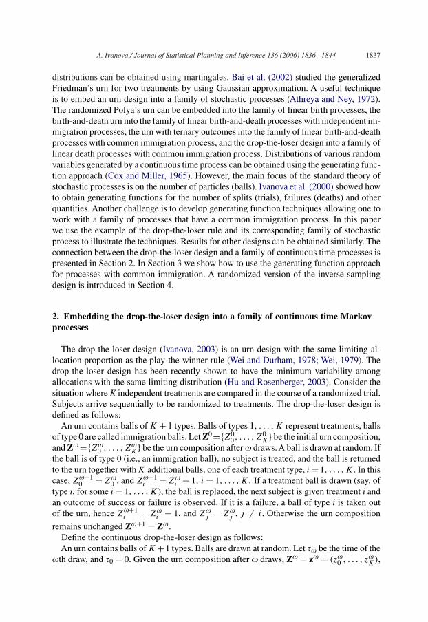
distributions can be obtained using martingales. Bai et al. (2002) studied the generalizedFriedman’s urn for two treatments by using Gaussian approximation. A useful techniqueis to embed an urn design into a family of stochastic processes (Athreya and Ney, 1972).The randomized Polya’s urn can be embedded into the family of linear birth processes, thebirth-and-death urn into the family of linear birth-and-death processes with independent im-migration processes, the urn with ternary outcomes into the family of linear birth-and-deathprocesses with common immigration process, and the drop-the-loser design into a family oflinear death processes with common immigration process. Distributions of various randomvariables generated by a continuous time process can be obtained using the generating func-tion approach (Cox and Miller, 1965). However, the main focus of the standard theory ofstochastic processes is on the number of particles (balls). Ivanova et al. (2000) showed howto obtain generating functions for the number of splits (trials), failures (deaths) and otherquantities. Another challenge is to develop generating function techniques allowing one towork with a family of processes that have a common immigration process. In this paperwe use the example of the drop-the-loser rule and its corresponding family of stochasticprocess to illustrate the techniques. Results for other designs can be obtained similarly. Theconnection between the drop-the-loser design and a family of continuous time processes ispresented in Section 2. In Section 3 we show how to use the generating function approachfor processes with common immigration. A randomized version of the inverse samplingdesign is introduced in Section 4.

2. Embedding the drop-the-loser design into a family of continuous time Markovprocesses

The drop-the-loser design (Ivanova, 2003) is an urn design with the same limiting al-location proportion as the play-the-winner rule (Wei and Durham, 1978; Wei, 1979). Thedrop-the-loser design has been recently shown to have the minimum variability amongallocations with the same limiting distribution (Hu and Rosenberger, 2003). Consider thesituation where K independent treatments are compared in the course of a randomized trial.Subjects arrive sequentially to be randomized to treatments. The drop-the-loser design isdefined as follows:

An urn contains balls of K + 1 types. Balls of types 1, . . . , K represent treatments, ballsof type 0 are called immigration balls. Let Z0={Z0

0, . . . , Z0K} be the initial urn composition,

and Z�={Z�0 , . . . , Z�

K} be the urn composition after � draws. A ball is drawn at random. Ifthe ball is of type 0 (i.e., an immigration ball), no subject is treated, and the ball is returnedto the urn together with K additional balls, one of each treatment type, i =1, . . . , K . In thiscase, Z�+1

0 = Z�0 , and Z�+1

i = Z�i + 1, i = 1, . . . , K . If a treatment ball is drawn (say, of

type i, for some i = 1, . . . , K), the ball is replaced, the next subject is given treatment i andan outcome of success or failure is observed. If it is a failure, a ball of type i is taken outof the urn, hence Z�+1

i = Z�i − 1, and Z�

j = Z�j , j �= i. Otherwise the urn composition

remains unchanged Z�+1 = Z�.Define the continuous drop-the-loser design as follows:An urn contains balls of K +1 types. Balls are drawn at random. Let �� be the time of the

�th draw, and �0 = 0. Given the urn composition after � draws, Z� = z� = (z�0 , . . . , z�

K),

1838 A. Ivanova / Journal of Statistical Planning and Inference 136 (2006) 1836–1844

generate K + 1 independent random variables U�0 , . . . , U�

K such that U�j has exponential

distribution with mean 1/z�j , j = 0, . . . , K . Let T�+1 = minj=0,...,K(U�

j ). If T�+1 = U�i ,

the ball type is i. Define ��+1 = �� + T�+1. If i = 0 (i.e., an immigration ball), the ballis returned to the urn together with K additional balls, one of each type, i = 1, . . . , K . Inthis case, Z�+1

0 = Z�0 , and Z�+1

i = Z�i + 1, i = 1, . . . , K . If a ball of type i = 1, . . . , K

is drawn, a patient is assigned to treatment i, and the ball is replaced. If the outcome is afailure a ball of type i is taken out of the urn, hence Z�+1

i = Z�i − 1, and Z�

j = Z�j ,j �= i.

Otherwise the urn composition remains unchanged, Z�+1 = Z�.Let qi , i = 1, . . . , K , be the probability of a failure on treatment i and pi = 1 − qi . The

continuous time process described by the urn defined above is equivalent to a family of Kcontinuous time linear death Markov processes with a common immigration process withrate a and independent death processes with death rates q1, . . . , qK (Ivanova, 2003). Wewill use the term “continuous urn” to refer to this family of continuous time processes.The process counting balls described by the urn above is equivalent to the drop-the-loserdesign.

3. Some distributional results for the continuous urn and the drop-the-loser design

Conventionally the behavior of stochastic processes is described by particles that split.In this paper we will use terminology of urn designs where balls are drawn from the urn.Let Zi(t) be the number of balls of type i at time t, Xi(t) be the number of draws of a ballof type i, followed by a success on treatment i, and Yi(t) be the number of draws of a ball oftype i followed by a failure on treatment i, so that the number of trials on the ith treatment,i = 1, . . . , K , is Ni(t) = Yi(t) + Xi(t). Let I (t), the common immigration process, be thenumber of draws of a ball of type 0 (immigration ball). By construction Zi(t)=Z0

i +I (t)−Yi(t). In this section our goal is to obtain the distributional results for the joint behaviorof Xi(t), Yi(t), Ni(t) and Zi(t). The standard stochastic processes literature is concernedwith Zi(t) only. However, a technique from Cox and Miller (1965, p. 265) can be extendedto obtain the differential equation for the joint probability generating function of all fourprocesses of interest, Xi(t), Yi(t), Ni(t) and Zi(t). We start by obtaining joint generatingfunction gXiYiNiZi (r, u, w, s, t)= E

{rXi(t)uYi(t)wNi(t)sZi(t)

}for the continuous urn with

a=0 and Z0i =1, i=1, . . . , K , i.e., when each process is generated by a single ball. Ivanova

and Flournoy (2001) described in detail how to obtain the partial differential equation forthe joint generating function. From Ivanova and Flournoy (2001), gXiYiNiZi (r, u, w, s, t) isthe solution of the partial differential equation:

�gXiYiNiZi (r, u, w, s, t)

�t= (−(1 − piwr)s + qiwu)

�gXiYiNiZi (r, u, w, s, t)

�s.

With the initial condition gXiYiNiZi (r, u, w, s, t = 0) = s, the solution of the equation is

gXiYiNiZi (r, u, w, s, t) = e−(1−pirw)t ((1 − pirw)s − qiwu) + qiwu

1 − pirw, (1)

where |r|�1, |u|�1, |w|�1, and |s|�1.


From (1) one can obtain various joint generating functions and the generating functionsgXi , gYi , gNi and gZi . For example,

gNi (w, t) = gXiYiNiZi (r = 1, u = 1, w, s = 1, t) = e−(1−piw)t (1 − w) + qiw

1 − piw.

The generating function in (1) corresponds to the process initiated by a single ball. LetGXiYiNiZi (r, u, w, s, t |Z0) = E{rXi(t)uYi(t)wNi(t)sZi(t)} be the joint generating functionfor the processes Xi(t), Yi(t), Ni(t) and Zi(t) generated by the continuous urn with initialcomposition Z0=(Z0

0=a, Z01, . . . , Z0

K). Theorem 3.1 (the proof is inAppendixA) describesa way of obtaining GXiYiNiZi (r, u, w, s, t |Z0) from the corresponding generating functionfor the continuous urn with initial composition (a = 0, Z0

1 = 1, . . . , Z0K = 1). Without loss

of generality, we state the theorem for GNi (w, t |Z0).

Theorem 3.1. The probability generating function for Ni(t), GNi (w, t |Z0), for the con-tinuous urn with initial composition Z0 = (Z0

0 = a, Z01, . . . , Z0

K) is

GNi (w, t |Z0) = e−at exp

{a

∫ t

0gNi (w, h) dh

}{gNi (w, t)}Z0

i .

One can use GNi (w, t |Z0) to obtain the expected number of trials on treatment i by timet. It is computationally easier to use the logarithm of the generating function, so-calledcumulant generating function:

E[Ni(t)]= � log GNi (w, t |Z0)

�w

∣∣∣∣w=1

=at

qi

− a

q2i

(1−e−qi t )+Z0i

1

qi

(1−e−qi t ). (2)

The variance of Ni(t) is

Var[Ni(t)] = d

dw

{w

d log GNi (w, t |Z0)

dw

}∣∣∣∣w=1

= a

q3i

{qit (2 − qi + 2(1 − qi)e−qi t ) − (4 − 3qi)(1 − e−qi t )}

+ Zi0

q2i

{(1 − qi)(1 − 2qite−qi t ) + qie

−qi t − e−2qi t }. (3)

Define N(t)=N1(t)+· · ·+NK(t), and let Si(t)=Ni(t)/N(t) be the allocation proportion

to treatment i by time t. From (2) we have Ni(t)/tP→

t→∞ a/qi . Hence the limit of Si(t) as t

goes to infinity is Di = (1/qi)/∑K

j=1 (1/qj ).So far we have been discussing the behavior of the process corresponding to one treatment

type. We now consider the joint behavior of the processes corresponding to two treatmenttypes i and j. Since there is a common immigration process, Ni(t) and Nj(t), i �= j , arenot independent.


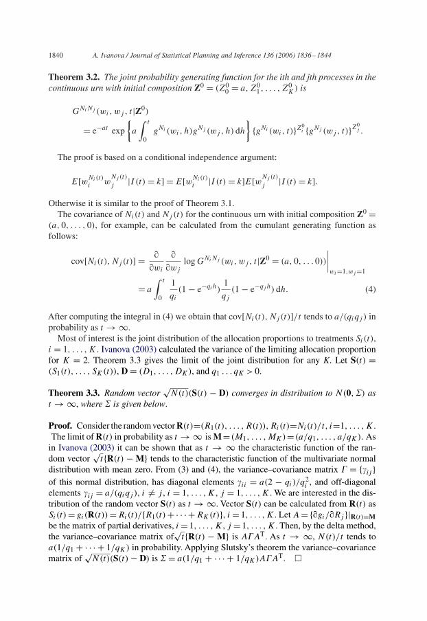
Theorem 3.2. The joint probability generating function for the ith and jth processes in thecontinuous urn with initial composition Z0 = (Z0

0 = a, Z01, . . . , Z0

K) is

GNiNj (wi, wj , t |Z0)

= e−at exp

{a

∫ t

0gNi (wi, h)gNj (wj , h) dh

}{gNi (wi, t)}Z0

i {gNj (wj , t)}Z0j .

The proof is based on a conditional independence argument:

E[wNi(t)i w

Nj (t)

j |I (t) = k] = E[wNi(t)i |I (t) = k]E[wNj (t)

j |I (t) = k].

Otherwise it is similar to the proof of Theorem 3.1.The covariance of Ni(t) and Nj(t) for the continuous urn with initial composition Z0 =

(a, 0, . . . , 0), for example, can be calculated from the cumulant generating function asfollows:

cov[Ni(t), Nj (t)] = �

�wi

�

�wj

log GNiNj (wi, wj , t |Z0 = (a, 0, . . . 0))

∣∣∣∣wi=1,wj =1

= a

∫ t

0

1

qi

(1 − e−qih)1

qj

(1 − e−qj h) dh. (4)

After computing the integral in (4) we obtain that cov[Ni(t), Nj (t)]/t tends to a/(qiqj ) inprobability as t → ∞.

Most of interest is the joint distribution of the allocation proportions to treatments Si(t),i = 1, . . . , K . Ivanova (2003) calculated the variance of the limiting allocation proportionfor K = 2. Theorem 3.3 gives the limit of the joint distribution for any K. Let S(t) =(S1(t), . . . , SK(t)), D = (D1, . . . , DK), and q1 . . . qK > 0.

Theorem 3.3. Random vector√

N(t)(S(t) − D) converges in distribution to N(0, �) ast → ∞, where � is given below.

Proof. Consider the random vector R(t)=(R1(t), . . . , R(t)),Ri(t)=Ni(t)/t, i=1, . . . , K .The limit of R(t) in probability as t → ∞ is M= (M1, . . . , MK)= (a/q1, . . . , a/qK). As

in Ivanova (2003) it can be shown that as t → ∞ the characteristic function of the ran-dom vector

√t{R(t) − M} tends to the characteristic function of the multivariate normal

distribution with mean zero. From (3) and (4), the variance–covariance matrix � = {�ij }of this normal distribution, has diagonal elements �ii = a(2 − qi)/q

2i , and off-diagonal

elements �ij = a/(qiqj ), i �= j , i = 1, . . . , K , j = 1, . . . , K . We are interested in the dis-tribution of the random vector S(t) as t → ∞. Vector S(t) can be calculated from R(t) asSi(t) = gi(R(t)) = Ri(t)/{R1(t) + · · · + RK(t)}, i = 1, . . . , K . Let A = {�gi/�Rj }|R(t)=Mbe the matrix of partial derivatives, i = 1, . . . , K , j = 1, . . . , K . Then, by the delta method,the variance–covariance matrix of

√t{R(t) − M} is A�AT. As t → ∞, N(t)/t tends to

a(1/q1 + · · · + 1/qK) in probability. Applying Slutsky’s theorem the variance–covariancematrix of

√N(t)(S(t) − D) is � = a(1/q1 + · · · + 1/qK)A�AT. �


For example, when K = 2, � is a matrix of rank one with diagonal elements equal toD1D2(2−q1−q2)/(q1+q2) and off diagonal elements equal to −D1D2(2−q1−q2)/(q1+q2). When K = 3, � has elements

�11 = D21D2

2D23q2

3 (2 − q1 − q2) + q22 (2 − q1 − q3) + 2q2q3(1 − q3)

1/q1 + 1/q2 + 1/q3,

�12 = D21D2

2D23−q2

3 (2 − q1 − q2) − q3(q1 + q2 − q1q2) + q1q2

1/q1 + 1/q2 + 1/q3,

with elements �22 and �33 defined similarly to �11, and elements �13 and �23 definedsimilarly to �12.

4. Randomized inverse sampling design

Consider the continuous urn with the following stopping rule: stop the sequence oftrials when � immigration balls have been drawn. By construction, process I (t) countingimmigrations (i.e., when an immigration ball is drawn from the urn) is a Poisson processwith rate a. Let the initial composition be Z0 = (a, 0, . . . , 0), a > 0, and let T� be the timeof �th immigration. Assume that immigration number � = 0 occurs at time T0 = 0. Weare interested in Xi(T�), Yi(T�), Ni(T�), and Zi(T�), the number of successes, failures,trials, and balls, respectively, at the moment when the �th immigration ball is drawn (but noballs are added to the urn following the �th immigration). Theorem 4 gives the general wayof obtaining the generating function for the processes generated by immigration with ratea > 0 from the corresponding generating function for the process generated by one ball.Without loss of generality we state the theorem for GZi (s, t |Z0). The proof is in AppendixB.

Theorem 4. The joint probability generating function for the processes counting successes,failures, trials, and balls, F

Zi� (r, u, w, s, t |Z0), for the urn with initial composition Z0 =

(a, 0, . . . , 0) at the time the �th immigration ball is drawn is

FZi� (s, t |Z0) =

∫ ∞

0

a�+1e−at

�!(∫ t

0gZi (s, h) dh

)�

dt ,

where gZi (s, t) is as defined in Section 3.

For example,

FZi

0 (s) = 1, FZi

1 (s) = 1 + as

a + qi

,

FZi

2 (s) = a2(a + qi)s2 + aqi(3a + 2qi)s + q2

i (3a + 2qi)

(a + qi)2(a + 2qi)

, etc.


The expected number of balls at the time the �th immigration ball is drawn is

E[Zi(T�)] = dFZi� (s|a)

ds

∣∣∣∣∣s=1

=∫ ∞

0

a�+1e−at

�! t�∫ t

0

dgZi (s, z)

ds

∣∣∣∣s=1

dzdt

= a

qi

[1 −

(a

a + qi

)�−1]

.

When a = 0 and Z0i > 0, i = 1, . . . , K , and sampling is done until the urn is empty, the

procedure is a well-known inverse sampling procedure (Haldane, 1945) where sampling isstopped when Z0

i failures are observed on each treatment. When a > 0, since Yi(t)= I (t)−Zi(t), the number of failures cannot be greater than the number of immigrations and thedesign above can be viewed as a randomized version of inverse sampling.

5. Discussion

Theoretical developments of this paper can be used to obtain important distributionalresults for many urn designs including the randomized Polya urn, the birth-and-death urn,the urn with ternary outcomes, and the drop-the-loser design. For example, these techniqueswere used to obtain an approximation of the bias of maximum likelihood estimates ofsuccess probabilities (Coad and Ivanova, 2001). Another important application is accessingthe variability of the allocation proportion for an urn design in the limit. Hu and Rosenberger(2003) showed that less variable procedures yield better power of treatment comparison, andsuggested comparing adaptive procedures based on variability of the allocation proportion.

Acknowledgements

The author is grateful to Stephen D. Durham for helpful discussions. The author thanksthe referees and an associate editor for their constructive comments.

Appendix A. Proof of Theorem 3.1

The following lemma is the basis of the proofs for the theorems of Section 3 and is ofindependent interest for computing conditional expectations, given the immigration process.

Lemma. Given I (t) = k and the immigration times, t1, . . . , tk ,

GNi (w, t |I (t) = k; t1, t2, . . . , tk) =k∏

j=1

gNi (w, t − tj ).

Proof. The result follows from the fact that conditional upon the immigration process, theprocesses generated by each of k immigration balls are independent. �


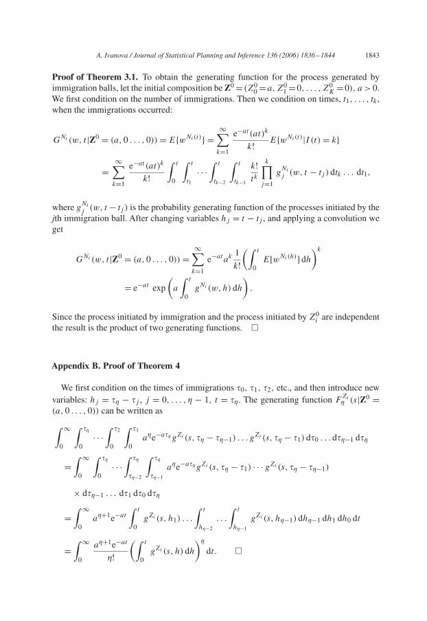
Proof of Theorem 3.1. To obtain the generating function for the process generated byimmigration balls, let the initial composition be Z0 = (Z0

0 =a, Z01 =0, . . . , Z0

K =0), a > 0.We first condition on the number of immigrations. Then we condition on times, t1, . . . , tk ,when the immigrations occurred:

GNi (w, t |Z0 = (a, 0 . . . , 0)) = E{wNi(t)} =∞∑

k=1

e−at (at)k

k! E{wNi(t)|I (t) = k}

=∞∑

k=1

e−at (at)k

k!∫ t

0

∫ t

t1

· · ·∫ t

tk−2

∫ t

tk−1

k!tk

k∏j=1

gNi

j (w, t − tj ) dtk . . . dt1,

where gNi

j (w, t − tj ) is the probability generating function of the processes initiated by thejth immigration ball. After changing variables hj = t − tj , and applying a convolution weget

GNi (w, t |Z0 = (a, 0 . . . , 0)) =∞∑

k=1

e−atak 1

k!(∫ t

0E[wNi(h)] dh

)k

= e−at exp

(a

∫ t

0gNi (w, h) dh

).

Since the process initiated by immigration and the process initiated by Z0i are independent

the result is the product of two generating functions. �

Appendix B. Proof of Theorem 4

We first condition on the times of immigrations �0, �1, �2, etc., and then introduce newvariables: hj = �� − �j , j = 0, . . . , � − 1, t = ��. The generating function F

Zi� (s|Z0 =

(a, 0 . . . , 0)) can be written as

∫ ∞

0

∫ ��

0· · ·

∫ �2

0

∫ �1

0a�e−a��gZi (s, �� − ��−1) . . . gZi (s, �� − �1) d�0 . . . d��−1 d��

=∫ ∞

0

∫ ��

0· · ·

∫ ��

��−2

∫ ��

��−1

a�e−a��gZi (s, �� − �1) · · · gZi (s, �� − ��−1)

× d��−1 . . . d�1 d�0 d��

=∫ ∞

0a�+1e−at

∫ t

0gZi (s, h1) . . .

∫ t

h�−2

. . .

∫ t

h�−1

gZi (s, h�−1) dh�−1 dh1 dh0 dt

=∫ ∞

0

a�+1e−at

�!(∫ t

0gZi (s, h) dh

)�

dt. �


References

Athreya, K.B., Ney, P.E., 1972. Branching Processes. Springer, Berlin.Bai, Z.D., Hu, F., 1999.Asymptotic theorems for urn models with nonhomogeneous generating matrices. Stochastic

Processes Appl. 80, 87–101.Bai, Z.D., Hu, F., Zhang, L.X., 2002. The Gaussian approximation theorems for urn models and their applications.

Ann. Appl. Probab. 12, 1149–1173.Coad, D.S., Ivanova, A., 2001. Bias calculations for adaptive designs. Sequential Anal. 20, 91–116.Cox, D.R., Miller, H.D., 1965. The Theory of Stochastic Processes. Wiley, New York.Durham, S.D., Flournoy, N., Li, W., 1998.Adaptive designs for maximizing the probability of a favorable response.

Canad. J. Statist. 479–495.Haldane, J.B.S., 1945. On a method of estimating frequencies. Biometrika 33, 222–225.Hu, F., Rosenberger, W.F., 2003. Optimality, variability, power: evaluating response adaptive randomization

procedures for treatment comparisons. J. Amer. Statist. Assoc. 98, 671–678.Ivanova, A., 2003. A play-the-winner-type urn design with reduced variability. Metrika 58, 1–13.Ivanova A., Flournoy, N., 2001. A birth and death urn for ternary outcomes: stochastic processes applied to urn

models. In: Charalambides, C.A., Koutras, M.V., Balakrishnan, N. (Eds.), Probability and Statistical Modelswith Applications. Chapman & Hall/CRC: Boca Raton, pp. 583–600.

Ivanova, A., Rosenberger, W.F., Durham, S.D., Flournoy, N., 2000. A birth and death urn for randomized clinicaltrials. Sankhya B 62, 104–118.

Rosenberger, W.F., 2002. Randomized urn models and sequential design. Sequential Anal. 21, 1–41.Smythe, R.T., 1996. Central limit theorems for urn models. Stochastic Processes Appl. 65, 115–137.Wei, L.J., 1979. The generalized Polya’s urn design for sequential medical trials. Ann. Statist. 7, 291–296.Wei, L.J., Durham, S., 1978. The randomized play-the-winner rule in medical trials. J. Amer. Statist. Assoc. 73,

840–843.

urn designs with immigration: useful connection with continuous time stochastic processes

Documents