unmanned aerial vehicle trajectory planning with … pennsylvania state university the graduate...
TRANSCRIPT

The Pennsylvania State University
The Graduate School
UNMANNED AERIAL VEHICLE TRAJECTORY PLANNING
WITH DIRECT METHODS
A Dissertation in
Aerospace Engineering
by
Brian Geiger
c⃝ 2009 Brian Geiger
Submitted in Partial Fulfillment
of the Requirements
for the Degree of
Doctor of Philosophy
August 2009
The dissertation of Brian Geiger was reviewed and approved∗ by the following:
Joseph F. Horn
Associate Professor of Aerospace Engineering
Dissertation Advisor, Chair of Committee
Lyle N. Long
Distinguished Professor of Aerospace Engineering and Mathematics
Jack W. Langelaan
Assistant Professor of Aerospace Engineering
Alok Sinha
Professor of Mechanical Engineering
George A. Lesieutre
Professor of Aerospace Engineering
Head of the Department of Aerospace Engineering
∗Signatures are on file in the Graduate School.

Abstract
A real-time method for trajectory optimization to maximize surveillance time ofa fixed or moving ground target by one or more unmanned aerial vehicles (UAVs)is presented. The method accounts for performance limits of the aircraft, intrinsicproperties of the camera, and external disturbances such as wind. Direct colloca-tion with nonlinear programming is used to implement the method in simulationand onboard the Penn State/Applied Research Lab’s testbed UAV. Flight test re-sults compare well with simulation. Both stationary targets and moving targets,such as a low flying UAV, were successfully tracked in flight test.
In addition, a new method using a neural network approximation is presentedthat removes the need for collocation and numerical derivative calculation. Neuralnetworks are used to approximate the objective and dynamics functions in theoptimization problem which allows for reduced computation requirements. Theapproximation reduces the size of the resulting nonlinear programming problemcompared to direct collocation or pseudospectral methods. This method is shownto be faster than direct collocation and psuedospectral methods using numerical orautomatic derivative techniques. The neural network approximation is also shownto be faster than analytical derivatives but by a lesser factor. Comparative resultsare presented showing similar accuracy for all methods. The method is modularand enables application to problems of the same class without network retraining.
iii

Table of Contents
List of Figures viii
List of Tables x
List of Symbols xi
Acknowledgments xiii
Chapter 1Introduction 11.1 Introduction . . . . . . . . . . . . . . . . . . . . . . . . . . . . . . . 11.2 Contributions . . . . . . . . . . . . . . . . . . . . . . . . . . . . . . 21.3 Methods Used in Trajectory Optimization . . . . . . . . . . . . . . 3
1.3.1 Indirect Methods . . . . . . . . . . . . . . . . . . . . . . . . 31.3.2 Direct Methods . . . . . . . . . . . . . . . . . . . . . . . . . 4
1.3.2.1 Direct Shooting . . . . . . . . . . . . . . . . . . . . 41.3.2.2 Direct Collocation . . . . . . . . . . . . . . . . . . 51.3.2.3 Pseudospectral Methods . . . . . . . . . . . . . . . 6
1.3.3 Mixed Integer Linear Programming . . . . . . . . . . . . . . 61.3.4 Dynamic Programming . . . . . . . . . . . . . . . . . . . . . 71.3.5 Genetic Algorithms . . . . . . . . . . . . . . . . . . . . . . . 7
1.4 UAV Specific Research . . . . . . . . . . . . . . . . . . . . . . . . . 81.4.1 Direct Collocation . . . . . . . . . . . . . . . . . . . . . . . 81.4.2 Pseudospectral Methods . . . . . . . . . . . . . . . . . . . . 91.4.3 Mixed Integer Linear Programming . . . . . . . . . . . . . . 91.4.4 Dynamic Programming . . . . . . . . . . . . . . . . . . . . . 101.4.5 Genetic Algorithms . . . . . . . . . . . . . . . . . . . . . . . 10
iv

1.4.6 ARL/PSU UAV Group Research . . . . . . . . . . . . . . . 11
Chapter 2Direct Nonlinear Trajectory Optimization 132.1 The Basic Problem . . . . . . . . . . . . . . . . . . . . . . . . . . . 132.2 Direct Collocation with Nonlinear Programming . . . . . . . . . . . 142.3 Pseudospectral Methods . . . . . . . . . . . . . . . . . . . . . . . . 172.4 Examples . . . . . . . . . . . . . . . . . . . . . . . . . . . . . . . . 21
2.4.1 Brachistochrone Example . . . . . . . . . . . . . . . . . . . 212.4.2 Moon Lander Example . . . . . . . . . . . . . . . . . . . . . 23
2.5 Receding Horizon . . . . . . . . . . . . . . . . . . . . . . . . . . . . 23
Chapter 3Neural Network Method 253.1 Introduction . . . . . . . . . . . . . . . . . . . . . . . . . . . . . . . 253.2 Method Motivation and Overview . . . . . . . . . . . . . . . . . . . 263.3 Previous and Related Research . . . . . . . . . . . . . . . . . . . . 273.4 Neural Network Formulation . . . . . . . . . . . . . . . . . . . . . . 28
3.4.1 Derivative Calculation . . . . . . . . . . . . . . . . . . . . . 313.5 Training . . . . . . . . . . . . . . . . . . . . . . . . . . . . . . . . . 34
Chapter 4UAV Path Planning Surveillance Problem 354.1 Equations of Motion . . . . . . . . . . . . . . . . . . . . . . . . . . 354.2 Discretization Scheme . . . . . . . . . . . . . . . . . . . . . . . . . 36
4.2.1 Direct Collocation and Pseudospectral Parameterization . . 374.2.2 Neural Network Approximation Parameterization . . . . . . 37
4.3 Constraints . . . . . . . . . . . . . . . . . . . . . . . . . . . . . . . 384.4 Objective Function . . . . . . . . . . . . . . . . . . . . . . . . . . . 38
4.4.1 Integrating External World Data . . . . . . . . . . . . . . . 434.4.2 Perspective Driven Surveillance . . . . . . . . . . . . . . . . 44
4.5 Neural Network Specific Details . . . . . . . . . . . . . . . . . . . . 444.5.1 Network Structure . . . . . . . . . . . . . . . . . . . . . . . 464.5.2 Neural Network Training . . . . . . . . . . . . . . . . . . . . 46
4.6 Simulation Results . . . . . . . . . . . . . . . . . . . . . . . . . . . 484.7 Convergence Results . . . . . . . . . . . . . . . . . . . . . . . . . . 56
4.7.1 Discretization Convergence . . . . . . . . . . . . . . . . . . . 574.7.2 Receding Horizon Convergence . . . . . . . . . . . . . . . . 59
4.8 Comparative Results . . . . . . . . . . . . . . . . . . . . . . . . . . 614.8.1 Training . . . . . . . . . . . . . . . . . . . . . . . . . . . . . 61
v
4.8.2 Results . . . . . . . . . . . . . . . . . . . . . . . . . . . . . . 624.8.2.1 Qualitative Comparison with other methods . . . . 634.8.2.2 Stationary Target . . . . . . . . . . . . . . . . . . . 644.8.2.3 Moving Target Results . . . . . . . . . . . . . . . . 654.8.2.4 Dual UAV Comparison . . . . . . . . . . . . . . . . 68
4.8.3 Comparative Conclusions . . . . . . . . . . . . . . . . . . . . 69
Chapter 5Real time implementation and Flight Test 755.1 UAV Testbed Description . . . . . . . . . . . . . . . . . . . . . . . 755.2 Implementation Issues & Initial Flight Tests . . . . . . . . . . . . . 81
5.2.1 Real-Time Implementation . . . . . . . . . . . . . . . . . . . 815.2.1.1 Hardware-in-the-Loop Simulation . . . . . . . . . . 82
5.3 Flight Test Results . . . . . . . . . . . . . . . . . . . . . . . . . . . 835.3.1 Stationary Target . . . . . . . . . . . . . . . . . . . . . . . . 845.3.2 Stationary Target in steady winds . . . . . . . . . . . . . . . 865.3.3 Tracking a moving ground target . . . . . . . . . . . . . . . 865.3.4 Tracking a flying UAV from above . . . . . . . . . . . . . . . 89
5.4 Integrated Target Tracking and Path Planning . . . . . . . . . . . . 945.4.1 Hardware-in-the-loop simulation description . . . . . . . . . 975.4.2 Path Planning . . . . . . . . . . . . . . . . . . . . . . . . . . 100
5.5 Discussion . . . . . . . . . . . . . . . . . . . . . . . . . . . . . . . . 101
Chapter 6Conclusions and Future Work 1036.1 Conclusions . . . . . . . . . . . . . . . . . . . . . . . . . . . . . . . 103
6.1.1 Collocation Methods and Flight Demonstration . . . . . . . 1036.1.2 Neural Network Approximation Method . . . . . . . . . . . 105
6.2 Future Work . . . . . . . . . . . . . . . . . . . . . . . . . . . . . . . 105
Appendix AAnalytical Derivations for the Direct Collocation Method 108A.1 Integrated control cost . . . . . . . . . . . . . . . . . . . . . . . . . 109A.2 Integrated distance-to-target cost . . . . . . . . . . . . . . . . . . . 109A.3 Integrated distance-to-target cost . . . . . . . . . . . . . . . . . . . 112A.4 Constraint Derivatives . . . . . . . . . . . . . . . . . . . . . . . . . 117
Appendix BNeural Network Weights, Biases, and Scaling for the UAV
Surveillance Problem 120
vi

B.1 Dynamics Network . . . . . . . . . . . . . . . . . . . . . . . . . . . 120B.2 Distance-to-target Network . . . . . . . . . . . . . . . . . . . . . . . 124B.3 Target-in-view Network . . . . . . . . . . . . . . . . . . . . . . . . . 127B.4 Scaling . . . . . . . . . . . . . . . . . . . . . . . . . . . . . . . . . . 130
Bibliography 132
vii

List of Figures
1.1 ARL/PSU Sig Kadet Senior UAV and Tankbot . . . . . . . . . . . 12
2.1 Illustration of direct collocation discretization scheme and defect . . 162.2 Illustration of Chebyshev pseudospectral method discretization . . . 192.3 Brachistochrone problem . . . . . . . . . . . . . . . . . . . . . . . . 212.4 Brachistochrone problem . . . . . . . . . . . . . . . . . . . . . . . . 222.5 Moon lander problem . . . . . . . . . . . . . . . . . . . . . . . . . . 24
3.1 Illustration of the segmented state trajectory . . . . . . . . . . . . . 29
4.1 Axes used in the homography . . . . . . . . . . . . . . . . . . . . . 404.2 Target-in-view cost functions . . . . . . . . . . . . . . . . . . . . . . 424.3 Path data illustration . . . . . . . . . . . . . . . . . . . . . . . . . . 434.4 Illustration of the perspective driven objective function . . . . . . . 454.5 Neural network illustrations for the target surveillance problem . . . 464.6 Common artificial neural network transfer functions . . . . . . . . . 474.7 Simulation of a single UAV and stationary target . . . . . . . . . . 494.8 Steady wind and target motion comparison. . . . . . . . . . . . . . 504.9 Simulation of a single UAV and fast moving target . . . . . . . . . 504.10 Simulation of a single UAV and slow moving target . . . . . . . . . 514.11 Simulation of a UAV pair and stationary target . . . . . . . . . . . 524.12 Distance from UAV to target . . . . . . . . . . . . . . . . . . . . . 524.13 Path planner simulation with road data . . . . . . . . . . . . . . . . 534.14 Path planner simulation with road data and fast target . . . . . . . 544.15 Simulation of a single UAV and stationary target (perspective driven) 554.16 Simulation of a single UAV and slow moving target (perspective
driven) . . . . . . . . . . . . . . . . . . . . . . . . . . . . . . . . . . 564.17 Observation ratio time history, stationary target . . . . . . . . . . . 574.18 Network training regression results (normalized) . . . . . . . . . . . 624.19 Stationary target comparison results . . . . . . . . . . . . . . . . . 644.20 Controls (longitudinal acceleration and bank angle) . . . . . . . . . 65
viii

4.21 Moving target comparison results, 10 ft/sec . . . . . . . . . . . . . 664.22 Moving target comparison results, 20 ft/sec . . . . . . . . . . . . . 674.23 Moving target comparison results, 25 ft/sec . . . . . . . . . . . . . 684.24 Moving target comparison results, 27 ft/sec . . . . . . . . . . . . . 694.25 Moving target comparison results, 35 ft/sec . . . . . . . . . . . . . 704.26 Relative path computation time (16-sec horizon) . . . . . . . . . . . 714.27 Relative path computation time (30-sec horizon) . . . . . . . . . . . 724.28 Ground track and coverage timeline for two UAVS and a target . . 72
5.1 The Applied Research Lab/Penn State UAV Testbed . . . . . . . . 775.2 Kadet UAV construction photos . . . . . . . . . . . . . . . . . . . . 785.3 Block diagram for the airborne and ground systems . . . . . . . . . 795.4 Airfield Photos and test target photos . . . . . . . . . . . . . . . . . 805.5 Stationary target observation in calm winds . . . . . . . . . . . . . 855.6 Stationary target observation with 5 knots wind from the west . . . 875.7 Observation of a walking person . . . . . . . . . . . . . . . . . . . . 885.8 Observation of a moving truck . . . . . . . . . . . . . . . . . . . . . 905.9 Initial acquisition of the target UAV from a parking orbit . . . . . . 915.10 Tracking of the target UAV around a rectangular path . . . . . . . 925.11 Tracking of the target UAV around a figure-8 pattern . . . . . . . . 945.12 Tracking of the target UAV around a figure-8 pattern (match speed) 955.13 Sample frame captures from the onboard video . . . . . . . . . . . . 965.14 Schematic of the hardware-in-the-loop simulation . . . . . . . . . . 975.15 Webcam HIL rig and calibration result . . . . . . . . . . . . . . . . 985.16 Comparison of actual and simulated aerial views . . . . . . . . . . . 995.17 Integrated path planner and target geolocation in HIL simulation . 1005.18 Histogram of processing times . . . . . . . . . . . . . . . . . . . . . 101
B.1 Dynamics network, Layer 1 . . . . . . . . . . . . . . . . . . . . . . 121B.2 Dynamics network, Layer 2 . . . . . . . . . . . . . . . . . . . . . . 121B.3 Dynamics network, Layer 3 . . . . . . . . . . . . . . . . . . . . . . 122B.4 Distance-to-target network, Layer 1 . . . . . . . . . . . . . . . . . . 124B.5 Distance-to-target network, Layer 2 . . . . . . . . . . . . . . . . . . 124B.6 Distance-to-target network, Layer 3 . . . . . . . . . . . . . . . . . . 125B.7 Target-in-view network, Layer 1 . . . . . . . . . . . . . . . . . . . . 127B.8 Target-in-view network, Layer 2 . . . . . . . . . . . . . . . . . . . . 128B.9 Target-in-view network, Layer 3 . . . . . . . . . . . . . . . . . . . . 128
ix

List of Tables
4.1 Objective Function Listing . . . . . . . . . . . . . . . . . . . . . . . 424.2 UAV performance constraints . . . . . . . . . . . . . . . . . . . . . 484.3 Target coverage convergence, 16 second horizon . . . . . . . . . . . 584.4 Target coverage convergence, 30 second horizon . . . . . . . . . . . 594.5 Target coverage convergence for increasing horizon, 1 sec node spacing 594.6 Target coverage convergence for increasing horizon, 2 sec node spacing 604.7 Target coverage convergence for increasing horizon, 4 sec node spacing 604.8 Path generation time (mean and standard deviation) . . . . . . . . 734.9 Path generation time relative to neural network method . . . . . . . 744.10 Target coverage (percentage of total simulation time) . . . . . . . . 74
5.1 Path planner configurations used in flight testing . . . . . . . . . . 835.2 UAV performance constraints . . . . . . . . . . . . . . . . . . . . . 84
A.1 Leading-point partials for the North direction for Jdist . . . . . . . . 112A.2 Trailing-point partials for the North direction for Jdist . . . . . . . . 112A.3 Leading-point partials for the East direction for Jdist . . . . . . . . 113A.4 Trailing-point partials for the East direction for Jdist . . . . . . . . 113
B.1 Dynamics network, Layer 1 . . . . . . . . . . . . . . . . . . . . . . 123B.2 Dynamics network, Layer 2 . . . . . . . . . . . . . . . . . . . . . . 123B.3 Dynamics network, Layer 3 . . . . . . . . . . . . . . . . . . . . . . 123B.4 Distance-to-target network, Layer 1 . . . . . . . . . . . . . . . . . . 126B.5 Distance-to-target network, Layer 2 . . . . . . . . . . . . . . . . . . 126B.6 Distance-to-target network, Layer 3 . . . . . . . . . . . . . . . . . . 126B.7 Target-in-view network, Layer 1 . . . . . . . . . . . . . . . . . . . . 129B.8 Target-in-view network, Layer 2 . . . . . . . . . . . . . . . . . . . . 129B.9 Target-in-view network, Layer 3 . . . . . . . . . . . . . . . . . . . . 129
x

List of Symbols
b Neural network bias vector
Cm Rotation matrix relating the camera axes to the UAV axes
D Pseudospectral method differentiation matrix
Δ Defect vector
g Acceleration due to gravity
Azimuth (rad)
H Homography matrix
J General scalar objective function
Jtiv “Target-in-view” objective function
K Camera intrinsic parameters matrix
� Elevation (rad)
k Active rows of the states Jacobian
ksc Active rows of state constraints Jacobian
N Number of nodes
n Number of UAVs
∇ Gradient operator
Pm Overall parameter vector
xi
p Position of the UAV with respect to the target, p = puav − ptgt
pc Control vector for n UAVs
ps State vector for n UAVs
Heading (rad)
q Number of targets
q Normalized pixel coordinates,[qx qy qz
]Tq Unnormalized pixel coordinates,
[qx qy qz
]Tpr Offset attraction point used with the perspective driven method
R Rotation matrix relating UAV body axes to world North-East-Down coor-dinates
s Nondimensional time
� Segment length (s)
Tℎ Horizon time (s)
u UAV Control vector
ua Longitudinal acceleration command (m/s2)
ui Control vector at the itℎ node
u� Bank angle command (radians)
Vt True airspeed (m/s)
xi State vector at the itℎ node
xt Target state vector
xu UAV state vector
W Neural network weight matrix
x, xt North position of UAV and target, respectively (m)
Y (⋅) Multi-input, feedforward artificial neural network
y, yt East position of UAV and target, respectively (m)
xii

Acknowledgments
I thank my advisor Dr. Joe Horn for guidance, advice, knowledge, and opportuni-ties given throughout both my Masters and Ph.D. work. I also thank my fellowstudents Len Lopes, Chris Hennes, Wei Guo, James Erwin, James Ross, and GregSinsley. I am especially grateful to Al Niessner. Without Al’s time and dedication,the Penn State UAV Team would not exist. Dr. Lyle Long and Dr. Jack Lange-laan also provided thoughts and advice for this project. I also thank Mike Roeckeland Dr. Richard Stern for guidance and financial support through the AppliedResearch Laboratory.
Finally, I deeply grateful to my fiancee Laura for her love and support.
xiii

Dedication
For my dad.. . . and my Grandma, from whom I got all my smarts.
xiv
Chapter 1Introduction
1.1 Introduction
Past and current research into UAV path planning has grown from the demand for
increased autonomous behavior capability from UAVs. Given the ability to plan a
trajectory based on human or sensor input, the UAV gains the capability to avoid
obstructions or other aircraft, track targets, optimize certain performance charac-
teristics such as endurance, and generally adapt to a dynamic situation. There has
been much research into numerical trajectory planning methods. These methods
can be divided into two main subsets: direct and indirect methods [1]. Indirect
methods are based on calculus of variations, while direct methods transform the
problem into a nonlinear programming problem. Generally, direct methods are
preferred over indirect methods due to simplicity. Indirect methods require the
formulation of the optimality conditions which can be complex. In addition, the
initial guess required to solve the resulting two-point boundary value problem can
be difficult to find. Direct methods do not require the derivation of optimality con-
ditions and can be solved as a nonlinear programming problem, for which methods
of solution are mature and relatively robust. Other methods of trajectory opti-
mization that are receiving increased attention today include genetic algorithms,
linear programming, and Lyapunov vector field methods.
The general trajectory optimization problem is described as a minimization of
a scalar function J subject to the equations of motion and optionally subject to
state trajectory constraints, control constraints, initial and final conditions, and
2
time constraints. The optimization problem is stated as such:
Find the optimal control that produces the optimal trajectory which minimizes
J = E(x(tf ), tf ) +
∫ tf
t0
F (x(t),u(t), t)dt (1.1)
subject dynamic equations
x =dx
dt= f(x(t),u(t), t) (1.2)
and state, control, and time (equality or inequality) constraints
cl ≤ c(x(t),u(t), t) ≤ cu (1.3)
Equation 1.1 is known as the Bolza cost functional. Its components are the Mayer
cost E(⋅), based on the final states and time, and the Lagrange cost F (⋅), based
on the integration along the state trajectory.
1.2 Contributions
The focus of this work is to develop a direct trajectory optimization method to be
used onboard an unmanned aerial vehicle in real-time for a surveillance task. One of
the main missions for UAVs is surveillance; an automatic method to generate a near
optimal path tailored to UAV and sensor hardware would be useful. Toward this
goal, a new real-time implementation of a direct collocation trajectory optimization
is presented. The method will be used to direct a UAV to maximize the time a
target is visible to an onboard camera, given the intrinsic parameters of the camera
(focal length, sensor size, orientation) and performance limits of the aircraft. The
real-time direct collocation method requires the use of analytic derivatives in the
constraint and objective derivative calculations which are used by the nonlinear
solver. The direct collocation method is tested in both simulation and in flight test
aboard the Applied Research Laboratory/Penn State (ARL/PSU) testbed UAV,
a heavily modified Sig Kadet Senior.
Because derivation of analytical derivatives for nontrivial nonlinear optimiza-
tion problems can be tedious, error-prone, and inflexible, a new neural network
3
based trajectory optimization method is also presented. The new method uses
feed-forward neural networks to approximate the dynamics and objective func-
tions. Feed-forward neural networks have been shown to be universal function
approximators; they can also be used to compute derivatives of the function they
are approximating. Using this property, the requirement for specific analytical
derivatives is removed for real-time operation with the neural network method. In
addition, the method is set up to remove collocation constraints which reduces the
problem size compared to the direct collocation and pseudospectral methods.
1.3 Methods Used in Trajectory Optimization
This section provides a quick overview of several methods currently used in tra-
jectory optimization.
1.3.1 Indirect Methods
The following is taken from [2]. Indirect methods are based on calculus of varia-
tions. The Hamiltonian is defined as
H = F (x,u, t) + �Tf (1.4)
where � adjoins the equations of motion constraints to the path objective func-
tion. For this brief overview, path constraints are neglected. The conditions for
optimality require that � satisfy
� = −∂H∂x
T
(1.5)
Additionally,∂H
∂u= 0 (1.6)
To obtain the adjoint vector, Equation 1.7 is integrated back in time starting from
the terminal condition given in Equation 1.8.
� = −(∂f
∂x
)T�−
[∂L
∂x
](1.7)

4
�(tf ) =∂E(xtf , ttf )
∂x(1.8)
Now, the optimal control can be computed over the time period by solving for u.
∂F
∂u
T
+∂f
∂u
T
� = 0 (1.9)
A numerical method used in solution of the above equations is called indirect
shooting. Indirect shooting iteratively solves the initial value problem and then
evaluates constraints to adjust initial conditions. It suffers from a high sensitivity
in the final results from small changes in the initial conditions. Betts [1] notes
that indirect shooting is best used when the dynamics are benign due to this high
initial condition sensitivity. An example of benign dynamics is a low-thrust orbit
trajectory where the states evolve slowly over a long time period. Finally, the
indirect shooting method requires a good initial guess which can be difficult to
obtain.
1.3.2 Direct Methods
Unlike indirect methods, direct methods can be used to solve the optimal con-
trol problem without derivation of the necessary conditions for optimality. Direct
methods operate by parameterizing the optimal control problem into a nonlin-
ear programming problem. Direct shooting methods integrate the state equations
directly between the nodes, while direct collocation methods use a polynomial ap-
proximation to the integrated state equations between the nodes. The following
sections give more detail.
1.3.2.1 Direct Shooting
The direct shooting method integrates the trajectory during the optimization. The
controls are piecewise between each point and can be piecewise constant, piecewise
linear, etc. An integration is performed using the piecewise control and the con-
straints are then evaluated. Based on some function of the constraints, the initial
conditions are adjusted and the process iterates until convergence [1]. A problem
with direct shooting is the sensitivity of the final state to minute changes in the

5
initial state. In order to overcome this, the integration can be restarted at interme-
diate points, thus breaking the trajectory into smaller segments to which the direct
shooting method can be more easily applied successfully. This is called multiple
shooting. Direct shooting has been widely used and was originally developed for
military space applications. [1].
1.3.2.2 Direct Collocation
Direct collocation differs slightly. It similarly discretizes the state trajectory into
a series of points and approximates the segments between the points with poly-
nomials. However, the difference between the first derivative of the interpolating
polynomial at the midpoint of a segment and the first derivative calculated from
the equations of motion at the segment midpoint is used as the defect. If this
defect approaches zero, the interpolating polynomials are ensured to be a good
approximation of the actual states.
Direct collocation was introduced by Dickmanns [3] as a general method for
solving optimal control problems. The direct collocation method has seen wide use
in spacecraft and satellite research. One of the first, Hargraves and Paris [4] ap-
plied it to a low earth orbit booster problem and a supersonic aircraft time-to-climb
problem. The method has also been used in determining finite-thrust spacecraft
trajectories [5] and optimal trajectories for multi-stage rockets in [6]. The problem
of low-thrust spacecraft trajectories is investigated in [7, 8, 9, 10]. In particular,
Reference [7] uses higher order Gauss-Lobatto quadrature rules instead of the orig-
inal trapezoidal and Simpson rules. This change allows for increased accuracy with
a reduced number of subintervals. The number of nonlinear programming param-
eters is smaller as a result. Rendezvous between two power limited spacecraft of
different efficiencies are studied in [8], showing that DCNLP can be applied to more
than one vehicle. Tang and Conway [9] studied low thrust interplanetary transfer
using the collocation method and noted that no a priori assumptions about the
optimal control solution were required to reach a solution. In [10], DCNLP is
identified to be in a general class of direct transcription methods. The relation-
ship between the original optimal control problem and the approximation afforded
by DCNLP is examined. The method has also been used in satellite detumbling
problems [11]. Again, the authors note that the initial guesses did not require any
6
information about the optimal control solution. Horie and Conway [12] studied
optimal aeroassisted orbital intercept using DCNLP. They noted that the direct
method allowed for easy inclusion of the complicated heating limit constraints
required for this problem compared to the two point boundary value problem for-
mulation, which is an indirect method. Additionally, they found that DCNLP has
an advantage over the two-point boundary value problem formulation in terms of
problem size and robustness.
Regardless of the use of direct shooting or direct collocation, the resulting
problem is a nonlinear programming problem for which there are many solvers
available. One such package is called SNOPT [13].
1.3.2.3 Pseudospectral Methods
Pseudospectral methods are a class of direct methods that discretize the states
and controls of a trajectory optimization problem with unevenly spaced nodes.
High-order (order equal to the number of nodes) polynomials of the Lagrange
interpolating form are used to approximate the states and controls over the interval
of interest. These methods offer increased accuracy with fewer nodes compared to
direct methods due to the uneven discretization scheme. Razzaghi and Elnagar [14]
were among the first to apply these methods to control of dynamic systems.
1.3.3 Mixed Integer Linear Programming
By writing the path planning problem as a series of discrete decisions between
linear constraints, the problem can be expressed as linear constraints on a mixture
of continuous and integer variables [15]. This formulation is know as a mixed
integer linear program (MILP). The constraints that give rise to nonlinearity when
solving aircraft path planning problems include limits on bank angle (turn rate) or
maximum airspeed. This nonlinearity can be avoided by modeling the aircraft as a
point mass acted on by a limited force and moving at a limited speed. In this way,
a turn rate limit can be imposed by merely limiting the magnitudes of the force
and velocity vectors that can act upon the point mass: !max = fmax/(mvmax).
A limit on the magnitude of a 2-d vector is nonlinear (a circle), but it can be
approximated linearly in the worst case by an inscribed square. For greater accu-

7
racy, more constraints can be imposed by inscribing a polygon with an increasing
number of sides in the limiting circle. Collision avoidance constraints can simply
be added by a rectangle around the aircraft. Once converted to MILP form, there
exists a good number of solvers to calculate the solution. Reference [15] gives a
good explanation of the method.
1.3.4 Dynamic Programming
Richard Bellman proposed this method in the 1950s. Its basis is breaking up the
optimization problem into smaller and smaller subproblems until a simple case is
reached that can be easily solved. Dynamic programming is most easily applied
to discrete systems, however by using the Hamilton-Jacobi-Bellman equation, dy-
namic programming can be used with continuous systems [2]. In essence, dynamic
programming applied to path planning is the calculation of the shortest path from
a starting point to an ending point over a group of connected nodes. The cost to
travel from one node to another adjacent node is the smallest decomposition pos-
sible and is simple to evaluate. Over the entire grid, the cost at all nodes to travel
to all other adjacent node is calculated. Then starting backwards from the ending
node, the minimal cost path to the starting node is calculated through summation.
1.3.5 Genetic Algorithms
Optimization using genetic algorithms has received increasing attention over the
past years in the UAV field. It was initially presented by Holland [16] in the 1970s.
This method starts with a population of possible solutions for a particular problem.
A function is applied to each individual solution in order to evaluate their ‘fitness’
(i.e. how well the individual solves the problem). Then, using a series of operations
inspired by genetics, a new population of solutions are generated. The basic genetic
operators are selection (based on fitness), recombination (mating), and mutation
(introducing small random changes). Genetic algorithms are global searches and
are less susceptible to getting stuck in local minima. No specific initial conditions
are required [17]. Reference [18] provides a tutorial in using genetic algorithms to
solve multi-objective problems. An interesting thing mentioned in this article is
the fact that using a genetic algorithm enables the discovery of multiple solutions

8
for different objective instead of using a weighted sum to combine them. A list of
survey papers on the overall field of genetic algorithms is also given in [18]. Several
uses of genetic algorithms in the UAV field are discussed in following section.
1.4 UAV Specific Research
1.4.1 Direct Collocation
Direct collocation has been applied to unmanned glider [19, 20] dynamic soaring
and powered UAV [21] dynamic soaring, wherein the aircraft recovers energy from
the atmosphere by cyclicly crossing wind velocity gradients. Dynamic soaring can
be cast into an optimal control problem by seeking an energy neutral trajectory, a
maximum altitude trajectory, or a minimum cycle time. The authors noted that
DCNLP was well suited to solving this problem.
In related work, Qi and Zhao [22] use direct collocation to minimize the thrust
required from an engine on a generic UAV when flying through a thermal. Using
a two-dimensional thermal vertical velocity profile, the method finds a path with
minimal constant thrust over a fixed distance, extracting energy from the thermal.
Two specific behaviors were observed. In the first behavior, the UAV airspeed
varies inversely with the thermal wind profile. With increasing vertical thermal
wind speed, aircraft speed decreases. This allows the UAV to fly slowly across the
upwelling air, while flying quickly through the downdraft. In the second behavior
the UAV flies in union with the thermal, rising and falling as it crosses the ther-
mal. The authors state these behaviours correspond with the patterns for optimal
thermal crossing in sailplanes. In summary, thermals can be used to maximize
either UAV range or speed.
Borrelli and others [23] investigated the method to provide centralized path
planning along with collision avoidance for UAVs. The collision avoidance applies
to both other aircraft and ground based obstacles. Both a collocation based non-
linear programming method and a mixed integer linear programming method were
investigated. An extensive set of tests were done across a large random problem
initial conditions. It was shown that the MILP method was always faster than
the NLP method, and that both methods produced optimal solutions with similar
9
costs. The MILP formulation uses simple linear dynamics, and the authors suggest
that future work should focus on using MILP to initialize an NLP method with
detailed dynamics.
Misovec, Inanc, Wohletz, and Murray [24] use a collocation method to gener-
ate flight paths while considering radar signature of the UAV. The method is not
DCNLP, rather it uses the NTG [25] package developed at Caltech (collocation,
but not solved with nonlinear programming). The work models radar detection
based on the attitude of the aircraft relative to the radar station. An interesting
characteristic of the detection model is that for paths flown directly toward the
radar site (‘nose-in’) were less detectable than paths that approached at an oblique
angle (‘nose-out’). Therefore, path heading plays an important part in detectabil-
ity. The path planner incorporated this dependence of detectability on relative
attitude to generate low observability paths while enabling the aircraft to reach all
waypoints.
1.4.2 Pseudospectral Methods
Williams [26] used the Legendre pseudospectral method for a three-dimensional,
terrain following path planner. He demonstrated that with the use of analytical
derivatives, the method could be made to run in real time. Yakimenko, Yunjun,
and Basset [27] examined pseudospectral methods for use with short-time aircraft
maneuvers and reported on several configurations of two MATLAB based opti-
mization packages that were suitable for real time operation. An sub-optimal but
very fast inverse dynamics method was also presented.
1.4.3 Mixed Integer Linear Programming
How, King, and Kuwata [28] use MILP on their testbed of 8 UAVs. The UAVs are
almost-ready-to-fly kits and use the Piccolo autopilot. A small part of their overall
system, MILP is the basis for a receding horizon path planner. The algorithm is
efficient enough to run in real time. All calculations are performed on the ground,
and waypoints for the optimal path are sent to the UAV over the Piccolo 900 MHz
link. The authors report several successful flight tests of two UAVs with the path
planner operating, including tests in significant winds and formation flight.
10
Toupet and Mettler [29] use MILP in combination with dynamic programming
for path planning of an unmanned helicopter. The area in which the helicopter is
to fly is decomposed into cells free of obstacles. Then the cost to go from one cell to
another can be calculated. Using cell size enables UAV performance constraints to
be introduced. The particular objective for this work was to minimize travel time.
Therefore, dynamic programming was used to find the shortest global path while
avoiding obstacles. This path was then used in the receding horizon trajectory
generation process to generate a local trajectory using MILP. The local trajectory
is not global and may not even reach to the target waypoint. However since
receding horizon control is used, the local trajectory will eventually include the
target waypoint. For a typical city block environment, the authors report real
time capability.
1.4.4 Dynamic Programming
Flint et al. [30] present an algorithm based on dynamic programming to generate
near-optimal paths for several UAVs to follow to search for target cooperatively.
The area to be searched is divided into a grid. UAV motion is modeled as a path
made up of lines connecting various points in the grid. The UAV moves by way of
a planning tree, and can make m decisions at each node in the tree (1 time step).
As dynamic programming works back from the final time, the method only solves
ahead by a certain number of steps, thus avoiding the problem of expanding the
search tree indefinitely. Other UAVs are treated as stochastic elements to model
the possibility that they will have observed the target before the subject UAV.
Thus the UAV would choose the path with the least likelihood of observations
from other UAVs. The authors showed that their algorithm identified significantly
more targets than a standard Zamboni search (so called because it resembles the
path a Zamboni machine take over an ice rink).
1.4.5 Genetic Algorithms
Anderson et al. [31] use a genetic algorithm to maximize the number of targets seen,
maximize the time they are seen, and minimize turn acceleration for a small UAV.
The research demonstrated the advantages of the genetic algorithms’ global search
11
compared to a method that only ensured local optimality. It also demonstrated
that GA outperforms a boundary reflection with random incidence angle method.
Shima et al. [32] present research on using genetic algorithms to solve a multiple
task assignment problem: assigning multiple UAVs to perform multiple tasks on
multiple targets. The method produces feasible solutions quickly compared to
more traditional methods. The authors mention that the method can make real
time operation feasible.
Nikolos et al. [33] use genetic algorithms for three dimensional path planning
over terrain. There are two parts to the planner: offline and online. The offline
planner generates a single B-spline path from the starting to the end points through
an environment with known obstacles. The online planner builds on this path
though radar readings to account for the unknown environment using a receding
horizon strategy. For both planners, a potential field is used around obstacles to
drive avoidance. Both versions were shown to be effective in generating a collision
free path through terrain. Furthermore, the online planner effectively avoided any
sensed obstacles, and produced a feasible path in a small number of generations,
which the authors mention would be feasible for real time operation.
1.4.6 ARL/PSU UAV Group Research
A quick overview of the research areas investigated by the ARL/PSU UAV Group
is given here. The main driver for the group’s research is the Applied Research
Lab’s Intelligent Controller architecture [34, 35, 36]. This software supports collab-
oration amongst heterogeneous vehicles, fuzzy decision making using continuous
inference networks, and overall mission control. Because the software is behavior
based, autonomous behaviors for the UAV needed to be developed. The focus of
this dissertation is the creation of a path planning algorithm that can serve as
a behavior for a target surveillance or search task. Initial results were presented
in [37]. Additional behaviors developed include vision based target identification
and geolocation [38, 39], range and vision sensor fusion for terrain generation and
target recognition [40], and basic collision avoidance for two UAVs (unpublished).
With these unmanned aircraft behaviors, and in addition to ground vehicle-specific
behaviors, the intelligent controller architecture can enable heterogeneous teams of

12
vehicles to communicate, delegate tasks based on vehicle capability, recover from
vehicle loss through reallocation of mission tasks, and enable sensor fusion with
data from multiple vehicles. Figure 1.1 is a photo of the Sig Kadet UAV next to
an ARL tankbot which will be used in a future collaboration demonstration. Both
vehicles support onboard operation of the Intelligent Controller software.
Figure 1.1. ARL/PSU Sig Kadet Senior UAV and Tankbot
Chapter 2Direct Nonlinear Trajectory
Optimization
Two common methods used in direct trajectory optimization are discussed in this
chapter. These methods are discussed for three reasons: (1) to define some of
the more popular methods in direct trajectory optimization (2) to compare with
the neural network approximation method in Chapter 3 (3) to provide a basis for
discussion on the application of each method to the UAV surveillance problem in
Chapter 4.
2.1 The Basic Problem
The basic problem structure of a trajectory optimization problem can be described
by finding the time dependent state vector x(t), time dependent control vector
u(t), initial time t0, and final time tf that minimize the Bolza cost functional.
J = E(xf , tf ) +
∫ tf
t0
F (x(t),u(t), t)dt (2.1)
The cost is subject to dynamics constraints,
x =dx
dt= f(x(t),u(t), t) (2.2)
14
state, control, and time (equality or inequality) constraints,
cl ≤ c(x(t),u(t), t) ≤ cu (2.3)
and possibly fixed initial and final conditions.
x(t0) = x0
x(tf ) = xtf
(2.4)
The general approach of direct, nonlinear trajectory optimization methods is to
discretize the above equations and convert them into a nonlinear programming
problem to allow an easier solution. Any number of the state or control variables
can have their initial or final values specified, and the final time can be fixed or
free to vary. Examples of two different methods of discretization and conversion
are the direct collocation method and the pseudospectral method.
2.2 Direct Collocation with Nonlinear Program-
ming
The direct collocation method uses equally spaced nodes in time to discretize the
optimization problem given in Equations 2.1-2.3. This work uses the method pre-
sented by Hargraves and Paris [4]. Segments between each node are approximated
with Hermite cubic interpolating polynomials. Hermite interpolating polynomials
are defined in terms of the endpoint values and first derivatives at the endpoints.
They are a natural fit with the optimization problem because the state vector x
and state derivatives x are readily available from the process model.
Let x(t) and u(t) be approximated by a piecewise Hermite cubic polynomial
xp(s) and a piecewise linear function up(s) where s ∈ [0, 1] is nondimensional
segment time: s = (t − ti)/� where t is time and ti is time at the start of the itℎ

15
segment. For the itℎ segment,
xpi(s) = [2(xi − xi+1) + xi + xi+1]s3
+ [3(xi+1 − xi)− 2xi − xi+1]s2
+ xis+ xi
upi(s) = ui + (ui+1 − ui)s
(2.5)
Given n segments, each of length � seconds, the problem is discretized with the
states and controls defined at each node (segment endpoints). Using x and x,
the Hermite cubics defining state behavior between the nodes are easily computed
using Equation 2.5.
To ensure the approximating polynomials accurately represent the equations
of motion, the derivative of the midpoint of each polynomial segment, xpi(0.5), is
compared to the equations of motion evaluated using the states at the interpolated
segment midpoint, f [xpi(0.5),upi(0.5)]. This “collocation” of the approximated
and actual derivatives gives the method its name. Carrying out the expansion for
the interpolated states and controls at the collocation points (accounting for the
nondimensionalized segment time1) results in:
xci = xpi(0.5) =1
2(xi + xi+1) +
�
8(xi − xi+1) (2.6)
uci = upi(0.5) = (ui + ui+1)/2 (2.7)
Additionally, the slope2 of the interpolated states at the collocation points are:
xci = − 3
2�(xi − xi+1)−
1
4(xi + xi+i) (2.8)
The defect is defined as
Δ = f(xci,uci)− xci (2.9)
When Δ is driven toward zero by choosing appropriate values of xi and xi+1, the
approximating polynomials will accurately represent the equations of motion if a
1Because the approximating polynomials are written in nondimensional time, xi = �f(xi,ui)
2Dimensional time derivatives are required here, so xci = xpi(0.5) = 1�ddsxpi
∣∣∣∣s=0.5
16
cubic polynomial is capable of doing so. Qualitatively, constraining the defect to
zero places a lower bound on the number of nodes required to accurately represent
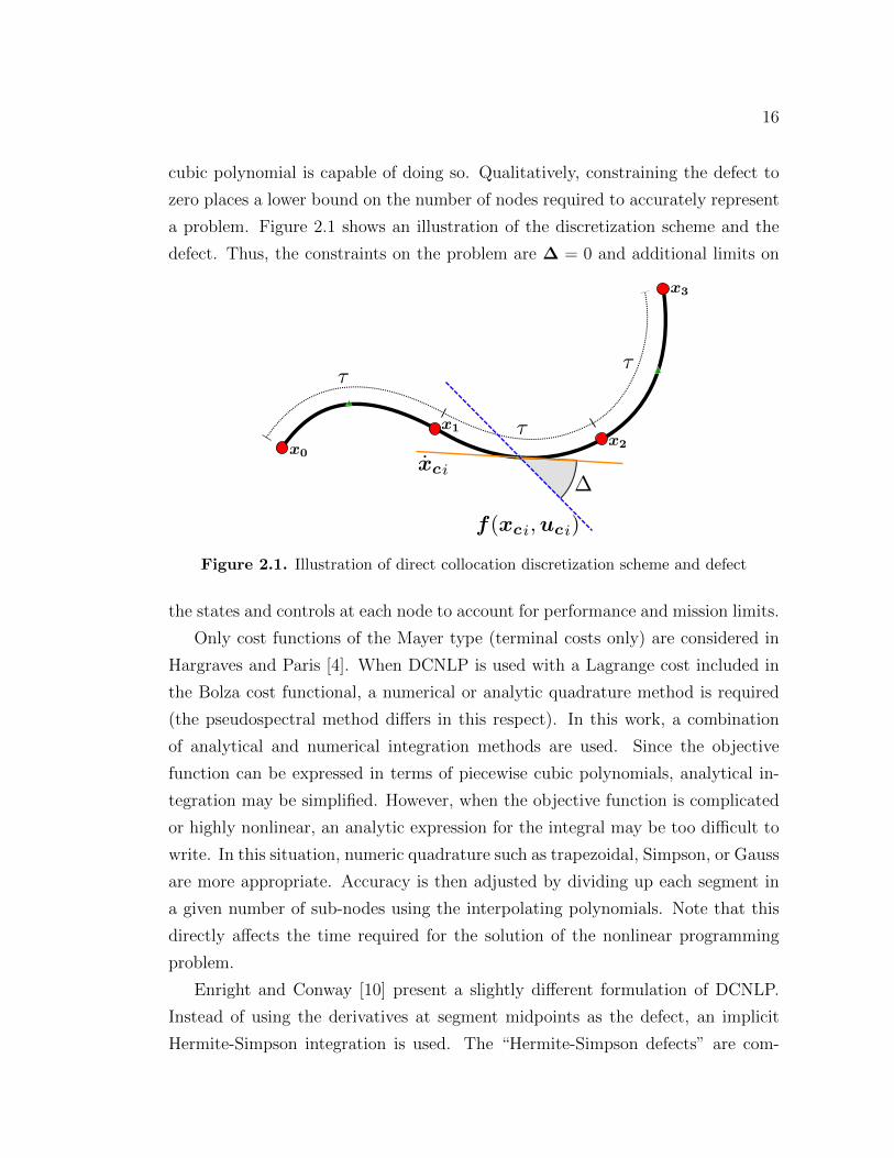
a problem. Figure 2.1 shows an illustration of the discretization scheme and the
defect. Thus, the constraints on the problem are Δ = 0 and additional limits on
62.63 px
Figure 2.1. Illustration of direct collocation discretization scheme and defect
the states and controls at each node to account for performance and mission limits.
Only cost functions of the Mayer type (terminal costs only) are considered in
Hargraves and Paris [4]. When DCNLP is used with a Lagrange cost included in
the Bolza cost functional, a numerical or analytic quadrature method is required
(the pseudospectral method differs in this respect). In this work, a combination
of analytical and numerical integration methods are used. Since the objective
function can be expressed in terms of piecewise cubic polynomials, analytical in-
tegration may be simplified. However, when the objective function is complicated
or highly nonlinear, an analytic expression for the integral may be too difficult to
write. In this situation, numeric quadrature such as trapezoidal, Simpson, or Gauss
are more appropriate. Accuracy is then adjusted by dividing up each segment in
a given number of sub-nodes using the interpolating polynomials. Note that this
directly affects the time required for the solution of the nonlinear programming
problem.
Enright and Conway [10] present a slightly different formulation of DCNLP.
Instead of using the derivatives at segment midpoints as the defect, an implicit
Hermite-Simpson integration is used. The “Hermite-Simpson defects” are com-

17
puted recursively from the preceding node, state derivatives at the preceding and
current node, and the interpolated midpoint. The defects differ from the original
formulation by a constant factor of 2�/3. The motivation for this change is to tie
in DCNLP with a general class of transcription methods that had been studied
previously and to mathematically provide a measure of the accuracy of the method.
2.3 Pseudospectral Methods
Spectral and pseudospectral methods were developed to solve partial differential
equations and historically used in fluid dynamics applications. The solution is
approximated by global, orthogonal polynomials. Spectral methods such as the
Galerkin or Tau methods seek to approximate the solution with a weighted sum
of a set of N continuous functions. The weighting coefficients are time depen-
dent. Pseudospectral or “collocation” methods use a set of discrete points by
which constant weighting coefficients3 can be calculated based on the underlying
approximating functions. The word “spectral” refers to the error convergence rate
with respect to an increasing number of nodes. Spectral convergence means that
error decreases faster than the rate of O(N−m) for any m > 0 (m is simply any
positive number)[41, 43, 44], or in simpler terms: error decreases exponentially
with increasing N .
With pseudospectral methods, states and controls are approximated with poly-
nomials of degree N in the Lagrange interpolating form. The various pseudospec-
tral methods use different discretization schemes for the collocation points and are
generally named for the scheme used. Some typical schemes include the Gauss
quadrature nodes, extrema of Legendre polynomials, roots of first derivatives of
Chebyshev polynomials (alternatively, the Chebyshev nodes are projections onto
the x-axis of equally spaced points on the circumference of the unit circle [44]).
The selection and implementation of the discretization schemes has consequences
in terms of the accuracy and smoothness of the costates [45]. Compared to equally
spaced nodes, these unequal node distributions offer increased performance and
3For example, the Galerkin spectral method uses an approximation in the form of f(x, t) =∑Nn=1 xi(t)Li(x) compared to xp(�) =
∑Nn=1 xiLi(t), which is the form used in the pseudospec-
tral method. [41, 42, 43]

18
improved numerical behavior.
The problem setup is similar to the direct collocation method in that opti-
mization is discretized. However, nodes unequally spaced in time are used and
the entire trajectory is approximated with a single high-order Lagrange interpo-
lating polynomial. The Chebyshev pseudospectral method[46, 47] is outlined here
as it is used in following chapters. Other pseudospectral methods follow similar
derivations [48, 49, 50, 45, 51].
The specific Chebyshev discretization is now discussed. The optimization prob-
lem is first transformed to the time interval on which the Chebyshev-Gauss-Lobatto
points are defined ([−1, 1]) so that the states with respect to time are given by
x[t(�)] where t(−1) = t0 and t(1) = tf .
t(�) = [(tf − t0)� + (tf + t0)]/2 (2.10)
The CGL points are used in Clenshaw-Curtis numerical quadrature, which is simi-
lar to Gaussian quadrature. These points are the extrema of the N tℎ order Cheby-
shev polynomial, which has a closed form expression.
�k = cos(�k/N) for k = 0, 1, . . . , N (2.11)
Choosing these interpolating points with the above distribution clusters more nodes
at the endpoints which avoids the Runge phenomenon (divergence of the approx-
imating polynomial at the endpoints). In addition, these nodes are used because
the max-norm of the corresponding polynomial approximation of a function over
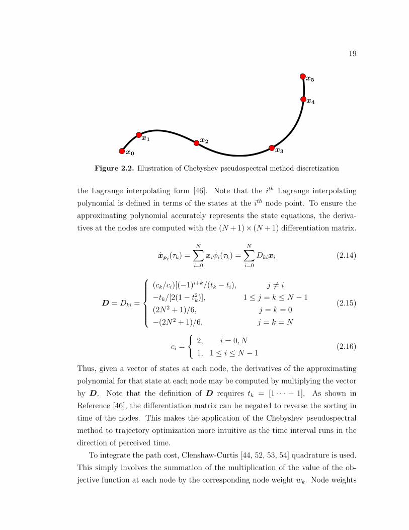
the CGL points is minimized [46]. Figure 2.2 shows a discretized trajectory with
six nodes.
Now, let x(t) and u(t) be approximated by the following form
xp(�) =N∑i=0
xi�i(t) (2.12)
up(�) =N∑i=0
ui�i(t) (2.13)
The state approximation at the itℎ node is given by an N tℎ order polynomial in
19
Figure 2.2. Illustration of Chebyshev pseudospectral method discretization
the Lagrange interpolating form [46]. Note that the itℎ Lagrange interpolating
polynomial is defined in terms of the states at the itℎ node point. To ensure the
approximating polynomial accurately represents the state equations, the deriva-
tives at the nodes are computed with the (N + 1)× (N + 1) differentiation matrix.
xpi(�k) =N∑i=0
xi�i(�k) =N∑i=0
Dkixi (2.14)
D = Dki =
⎧⎨⎩(ck/ci)[(−1)i+k/(tk − ti), j ∕= i
−tk/[2(1− t2k)], 1 ≤ j = k ≤ N − 1
(2N2 + 1)/6, j = k = 0
−(2N2 + 1)/6, j = k = N
(2.15)
ci =
{2, i = 0, N
1, 1 ≤ i ≤ N − 1(2.16)
Thus, given a vector of states at each node, the derivatives of the approximating
polynomial for that state at each node may be computed by multiplying the vector
by D. Note that the definition of D requires tk = [1 ⋅ ⋅ ⋅ − 1]. As shown in
Reference [46], the differentiation matrix can be negated to reverse the sorting in
time of the nodes. This makes the application of the Chebyshev pseudospectral
method to trajectory optimization more intuitive as the time interval runs in the
direction of perceived time.
To integrate the path cost, Clenshaw-Curtis [44, 52, 53, 54] quadrature is used.
This simply involves the summation of the multiplication of the value of the ob-
jective function at each node by the corresponding node weight wk. Node weights

20
are given in [46, 47]. The discretized formulation of the optimization problem can
now be written as: Find the parameters
x0,x1, . . . ,xN , u0,u1, . . . ,uN (2.17)
that minimize
J = E(xN , tf ) +tf − t0
2
N∑i=0
F (xi,ui, ti)wi (2.18)
subject to
2/(tf − t0)XD − f(x,u, t) = 0 (2.19)
cl ≤ c(xi,ui, ti) ≤ cu (2.20)
An abuse of notation for Equation 2.19 is that X is a matrix of column vectors
x0 . . .xN ; the states at each node. Furthermore, f(x,u, t) is actually computing
a matrix of x column vectors (x0 . . . xN ; the state derivatives at each node). Ad-
ditionally, Equation 2.19 can be rewritten in an equivalent form to take advantage
of linear versus nonlinear constraints [55].
Xoffdiag(D) +Xdiag(D)− tf − t02
f(x,u, t) = 0 (2.21)
In this form, X multiplied by the off-diagonals of D is always constant and can
be represented as linear constraints in the nonlinear programming problem. Solv-
ing a problem with linear constraints is usually faster than equivalent nonlinear
constraints. The number of nonlinear constraints is significantly reduced and only
consists of X multiplied by the matrix formed from the diagonal of D. To see why
this is true, note that only the states at a particular node affect the state deriva-
tives at a particular node. This corresponds to the diagonal of D post-multiplying
X. Thus the off-diagonals post-multiplying X are constant and can be treated as
linear constraints.
21
2.4 Examples
2.4.1 Brachistochrone Example
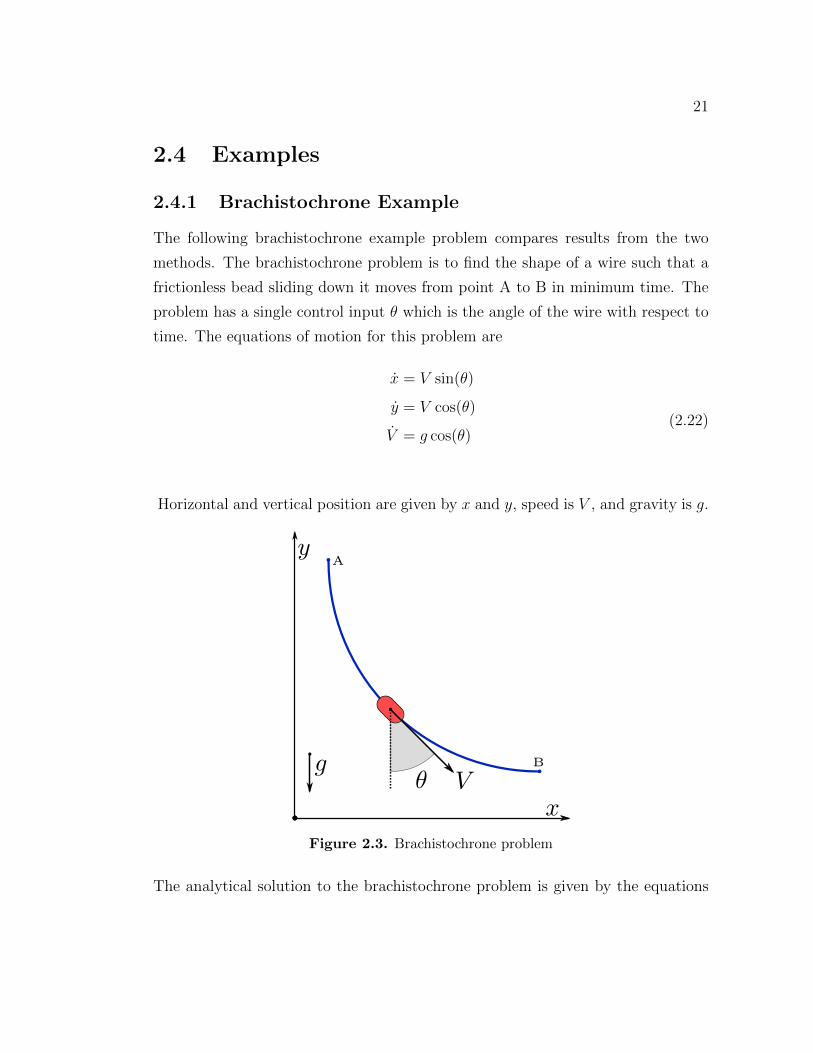
The following brachistochrone example problem compares results from the two
methods. The brachistochrone problem is to find the shape of a wire such that a
frictionless bead sliding down it moves from point A to B in minimum time. The
problem has a single control input � which is the angle of the wire with respect to
time. The equations of motion for this problem are
x = V sin(�)
y = V cos(�)
V = g cos(�)(2.22)
Horizontal and vertical position are given by x and y, speed is V , and gravity is g.
Figure 2.3. Brachistochrone problem
The analytical solution to the brachistochrone problem is given by the equations

22
of a cycloid.
�(�) =�
2
�
�f
x(�) = (g�f/�)(� − (�f/�) sin[2�(�)])
y(�) = (2g� 2f /�2) sin[�(�)]2
(2.23)
Given the desired final horizontal position, �f can be computed.
�f =
√�x(�f )
g(2.24)
Letting x0 = y0 = 0, xf = 5, and g = 1.0, the optimal final time is√
5� =
3.9633272976. Eleven nodes are used for both methods. The direct collocation
method results in an optimal time of 3.9633289715 with an absolute error of 1.7×10⁻⁶. The Chebyshev method gives an optimal time of 3.9633272972 with an
absolute error of 4× 10⁻¹⁰. The trajectory and control time history are shown in
Figure 2.4. Note that for the x-y plot, spacing is distorted because the states are
not shown with respect to time.
0 1 2 3 4 5−3.5
−3
−2.5
−2
−1.5
−1
−0.5
0
X position
Y p
ositi
on
AnalyticPseudospectralDirect Collocation
(a) x and y trajectory
0 0.5 1 1.5 2 2.5 3 3.5 40
0.2
0.4
0.6
0.8
1
1.2
1.4
1.6
Time (sec)
The
ta
AnalyticPseudospectralDirect Collocation
(b) Control time history
Figure 2.4. Brachistochrone problem
23
2.4.2 Moon Lander Example
The moon lander problem [56] is a simple three state system in which the objective
is to land softly given an initial height, vertical speed, and mass while using min-
imum fuel. The single control is vertical thrust. Mass decreases as fuel is burned
off when the thruster is engaged. The state equations are
ℎ = v
v = −g +T
m
m = − T
Ispg
(2.25)
Thrust, T is bounded from 0 to Tmax. Gravity g and specific impulse Isp are given
constants. Initial conditions are given and the desired final conditions for an intact
landing are ℎf = vf = 0. Additionally, the lander must not run out of fuel, so
mf > 0. To minimize fuel burn, final mass is maximized.
The problem setup here is similar to [46]. Choosing g = Isp = 1.0, Tmax = 1.1,
ℎ0 = m0 = 1.0, and v0 = −0.05, the problem is solved with both methods using
21 nodes. The direct collocation method results in a final mass of mf = 0.1804
while the pseudospectral method results in mf = 0.1800. The direct collocation
method is able to more accurately capture the optimal bang-bang control than the
pseudospectral method because the unevenly spaced nodes of the pseudospectral
method are less dense in the middle interval which leads to increased approxi-
mation errors at the control switch point. However, multi-phase schemes for the
pseudospectral method could eliminate this by adding a free phase boundary cor-
responding to the control switch point. Figure 2.5 shows a height-velocity diagram
and thrust control time history.
2.5 Receding Horizon
In order to accommodate the real-time operation constraints on the trajectory
optimization, a receding horizon approach is used. Instead of solving for the entire
trajectory over the length of the mission duration, only the trajectory over a smaller
horizon time Tℎ is computed. After a certain amount of time passes (the horizon

24
−1 −0.8 −0.6 −0.4 −0.2 00
0.1
0.2
0.3
0.4
0.5
0.6
0.7
0.8
0.9
1
Vertical Speed
Hei
ght
PseudospectralDirect Collocation
(a) Height vs. vertical speed
0 0.2 0.4 0.6 0.8 1 1.2 1.4 1.6 1.80
0.2
0.4
0.6
0.8
1
1.2
1.4
Time (sec)
Thr
ust C
ontr
ol
PseudospectralDirect Collocation
(b) Thrust control time history
Figure 2.5. Moon lander problem
update interval, Tu, the optimization is repeated with new initial conditions. This
affords two advantages: (1) changing situational information can be accounted for
in the optimization (2) a compromise of accuracy versus computation time can
be made. By decreasing Tℎ, the number of varied parameters in the optimization
can be reduced, decreasing required computation time. Comparisons will be made
between long and short horizon times to check for optimization convergence.

Chapter 3Neural Network Method
3.1 Introduction
A limiting factor in real-time trajectory optimization is computational require-
ments. A main driver of the computational requirement is the calculation of ob-
jective and constraint derivatives for use in the solution of the nonlinear program.
Generally, these derivatives are calculated through numerical methods which are
slow and can be inaccurate. Analytical derivative calculation will provide signifi-
cant speedup, but are tedious and error-prone. There are methods of solution of
aircraft trajectory optimization problems that do not require the use of derivatives
such as the work by Yakimenko [57]. However, initial and final states must be
specified in that method. This section however focuses on a neural network ap-
proximation method that removes the need to numerically compute the objective
and constraint derivatives and removes the need for collocation, thus reducing the
nonlinear programming problem size. Similar to a multiple shooting method, the
controls are parameterized and state equations are integrated between nodes. The
method will be described in this chapter and is applied to a UAV surveillance
problem in comparison to the methods presented in the previous chapter. The
basis for this method was originally presented in Reference [58]. Extended results
will appear in Reference [59].
26
3.2 Method Motivation and Overview
Direct collocation [4] and pseudospectral methods [46, 50, 48], while different, share
one common characteristic in that the dynamics are collocated at discrete points
along the trajectory. This allows the conversion of the continuous optimization
problem to a discrete, nonlinear programming problem using approximating poly-
nomials of various forms. Collocation is used to ensure the approximating poly-
nomials are accurate representations of the states’ behavior between the discrete
nodes. However, collocation adds additional constraints to the nonlinear program-
ming problem. These constraints directly add to the computational cost of the
problem because nonlinear solvers generally make use of the constraint derivatives
with respect to the varied parameters. Numerical derivatives computed with fi-
nite differencing are slower and less accurate compared to analytical derivatives. In
addition, the finite differencing step size must be chosen with care. Derivative accu-
racy directly influences the speed and accuracy of an optimal solution. Automatic
methods for computing derivatives that match analytic accuracy exist[60, 61], but
are generally only moderately faster than finite differencing and do not approach
the performance of analytic derivatives.
The neural network approximation method removes the need for collocation
and numeric or automatic derivative calculation by approximating the dynamics
with a neural network over a small, given time period. The trajectory is then built
recursively by chaining these segments together. The objective function over the
trajectory is computed in the same manner. This allows the dynamics constraint
to be met in the offline network training phase, avoiding the collocation require-
ment when solving the problem. An additional advantage of the neural network
approximation is that the objective and constraint derivatives are easily calculated
analytically for any feedforward network. Hornik, Stinchombe, and White showed
the existence of a neural network with one hidden layer can be a universal approx-
imator given certain conditions [62, 63, 64]. If a smooth hidden layer is used, they
show that the network converges to the function’s first derivatives as well. Only
the existence of such a network is proven; there is no theory on how many neurons
should be used to match a particular funtion. Thus it is important to check for
convergence after training. Alternatively, Basson and Engelbrecht [65] present a

27
method for explicitly learning the first derivatives along with the target function.
This may provide an alternative to simply relying on network convergence.
Note that currently the method is limited to problems with fixed final time,
however, it could be applied to free time problems by discretizing along one of the
states with a fixed final value and training the network appropriately. Work in
inverting a feedfoward neural network [66] such that the desired outputs are used
to compute the inputs may also facilitate using the method in this situation.
3.3 Previous and Related Research
Some previous research using neural networks in trajectory optimization is now
discussed. A large body of work exists on using neural networks to directly solve
nonlinear programming problems. In 1957, Dennis [67] proposed the idea of solving
linear and quadratic programming problems by implementing them with analog
electrical networks. These networks provided very fast solutions. Out of this work
lead to the idea of using a neural network as a dynamic system whose equlibrium
point is the solution to the linear, quadratic, or nonlinear programming problem.
Effati and Baymani [68] propose a method for quadratic programming (sequen-
tial quadratic programming is widely used method in solving nonlinear programs)
that uses a Hopfield model of a neural network. The network is treated as a dy-
namic system that converges over time to the optimal solution of the primal and
dual problems. Reifman and Feldman [69] discuss a method in which the inverse
dynamics are modeled by a feed-forward network in order to convert the nonlin-
ear programming problem to an unconstrained form and solve it via a bisection
method. Many others have reported results in this area. However, our method is
only tangentially related to this area of research.
Work by Niestroy [70], Seong and Barrow [71], and Peng et al. [72] use a network
to approximate various optimal controllers; this is known as “neural dynamic opti-
mization”. Given the system model, the network weights and biases are optimized
offline to produce an optimal controller that minimizes an objective function of the
states and controls. The trained network is then used online to control the system.
The authors are in general agreement that the resulting controller is robust to
modeling errors. However, it may be difficult to change the controller without re-
28
training the network if the dynamics or objective changes. Yeh [73] approximated
the strength of concrete given various ingredients and experimental data with a
neural network and then used the network in a nonlinear programming problem to
optimize the mix. The network was only used to provide an experimental model.
Similarly, Inanc et al. [74] use a neural network to approximate the signature and
probability detection functions of a UAV for a low-observable trajectory generation
framework. Specifically, they used the neural network to approximate tabular data
in order to provide a differentiable function for the trajectory optimization. The
authors report that the neural network approximation increases the smoothness of
the resulting trajectory compared to a B-spline approximation. While the neural
network required fewer constraints, the authors do not give any computation time
comparison.
3.4 Neural Network Formulation
As before, the basic optimization problem is one of minimizing an objective func-
tion with any type of nonlinear constraints. Consider the nonlinear dynamic system
given in Equation 2.2 and the nonlinear constraints given in Equation 2.3
x = f(x,u) (3.1)
c(x,u) ≤ 0 (3.2)
where x and u are the state and control input vectors. We seek the control input
u(t) that minimizes a scalar objective function of the form:
J =
∫ tf
t0
(x,u)dt (3.3)
In general, any number of the state variables can have their initial values, x0, or
their final values, xtf , specified, and the final time tf must be fixed. Because the
neural network approximation method is currently limited to problems where the
final time is known, tf is specified, but the final state vector is free to vary. A
receding horizon approach, with horizon time Tℎ, is used to make the computation
feasible in real time and to incorporate new information as conditions change.
29
The trajectory is discretized into n equal segments of length � seconds, where
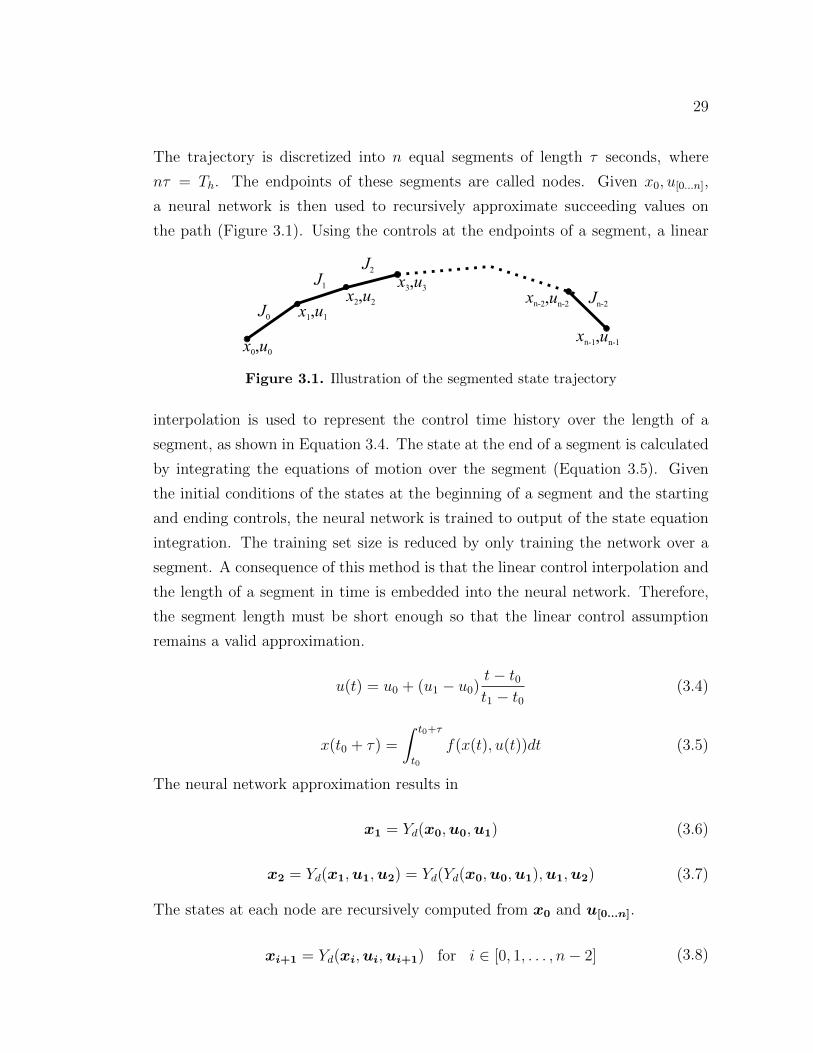
n� = Tℎ. The endpoints of these segments are called nodes. Given x0, u[0...n],
a neural network is then used to recursively approximate succeeding values on
the path (Figure 3.1). Using the controls at the endpoints of a segment, a linear
Figure 3.1. Illustration of the segmented state trajectory
interpolation is used to represent the control time history over the length of a
segment, as shown in Equation 3.4. The state at the end of a segment is calculated
by integrating the equations of motion over the segment (Equation 3.5). Given
the initial conditions of the states at the beginning of a segment and the starting
and ending controls, the neural network is trained to output of the state equation
integration. The training set size is reduced by only training the network over a
segment. A consequence of this method is that the linear control interpolation and
the length of a segment in time is embedded into the neural network. Therefore,
the segment length must be short enough so that the linear control assumption
remains a valid approximation.
u(t) = u0 + (u1 − u0)t− t0t1 − t0
(3.4)
x(t0 + �) =
∫ t0+�
t0
f(x(t), u(t))dt (3.5)
The neural network approximation results in
x1 = Yd(x0,u0,u1) (3.6)
x2 = Yd(x1,u1,u2) = Yd(Yd(x0,u0,u1),u1,u2) (3.7)
The states at each node are recursively computed from x0 and u[0...n].
xi+1 = Yd(xi,ui,ui+1) for i ∈ [0, 1, . . . , n− 2] (3.8)

30
Similarly, to approximate the objective function, the neural network is trained
to approximate the value of the objective along a segment. Again, the value of the
objective function along such a segment depends only on the initial state and the
control history.
J0 =
∫ t0+�
t0
(x,u)dt (3.9)
Approximated by the neural network:
J0 = YJ(x0,u0,u1) (3.10)
The objective function over the length of the horizon time can be built up by using
the state at the end of a previous segment as the initial condition for the next.
Thus, the objective function value depends only on the initial state at the first
node and the controls at each node.
J =n−2∑i=0
Ji =n−2∑i=0
YJ(xi,ui,ui+1) (3.11)
The optimization problem is reduced from finding all of the states and controls
to simply finding the controls. It is no longer a collocation problem because the
approximating functions, be they Hermite cubics or N tℎ degree Lagrange polyno-
mials, have been replaced by the neural network. The ‘defect,’ which is used in
the direct collocation and pseudospectral methods to ensure the approximating
polynomials accurately represent the true equations of motion, is now accounted
for in the neural network training. Multiple objective functions can be combined
in a weighted sum. Overall limits on the controls are present in the optimization
problem and do not require additional optimization parameters. To apply limits
on the state variables, additional optimization parameters are required. It is then
advantageous to write the dynamic equations to avoid state limit requirements
or to automatically adhere to state limits. Once the problem is parameterized,
SNOPT [13] or another suitable nonlinear solver is used to solve the nonlinear
programming problem.

31
3.4.1 Derivative Calculation
By approximating the problem with neural networks, the Jacobians of the system
equations, objective, and constraint functions become a straightforward calcula-
tion. Assuming the network is well trained, the approximated derivatives will
converge to the target function derivatives [62, 63, 64]. The current work uses a
three layer feed forward network: one input layer, one hidden layer, and one output
layer. The transfer functions used are linear, hyperbolic tangent sigmoid, and log-
arithmic sigmoid. The corresponding functions in the Neural Network Toolbox for
MATLAB are purelin, tansig, and logsig. Consider a three-layer feed-forward
network with weight matrices W[i,ℎ,o] and bias vectors b[i,h,o] corresponding to the
inner, hidden, and outer layers, respectively. Layer transfer functions are denoted
by y(⋅). In a feed-forward network, each node in a particular layer receives the
weighted sum of the output from all nodes in the previous layer. Given input
vector x, the equation for network output z is
z = y(Woy(Wℎy(Wix+ bi) + bh) + bo) (3.12)
The hyperbolic tangent sigmoid and its derivative is given by
y(x) =2
1 + e−2x− 1 (3.13a)
∇y(x) = 1− x2 (3.13b)
The logarithmic sigmoid and its derivative is given by
y(x) =1
1 + e−x(3.14a)
∇y(x) = x(1− x) (3.14b)
The linear transfer function is simply y(x) = x. Using the chain rule, the deriva-
tives of the entire network can be easily computed. For the three layer network,
the derivatives are
∇z = (diag(∇yo)Wo)(diag(∇yh)Wℎ)(diag(∇yi)Wi) (3.15)
32
where ∇y[i,h,o] denote the gradient of the transfer function of the input, hidden
and output layers, respectively. The diag function creates a diagonal matrix from
the vector argument. Note that this is only the derivative for one segment of the
overall trajectory. To compute the total derivative, the chain rule must be applied
again across all segments.
Recall that the state equations, objective, and constraint functions are recur-
sively calculated. Thus the state and controls at the first node affect every deriva-
tive for the following nodes. The objective gradient calculation is expanded to
illustrate the procedure. Consider a path with n nodes with m states and p con-
trols at each node. Let the objective function value for the itℎ segment be given by
Ji = f(xi,ui,ui+1) for i ∈ [0, 1, . . . , n− 2], and the states at the itℎ node be given
by xi = g(xi−1,ui−1,ui) for i ∈ [1, 2, . . . , n− 1]. The initial state x0 and control
u0 are given and control vectors u0 . . .un−1 are computed by the optimization.
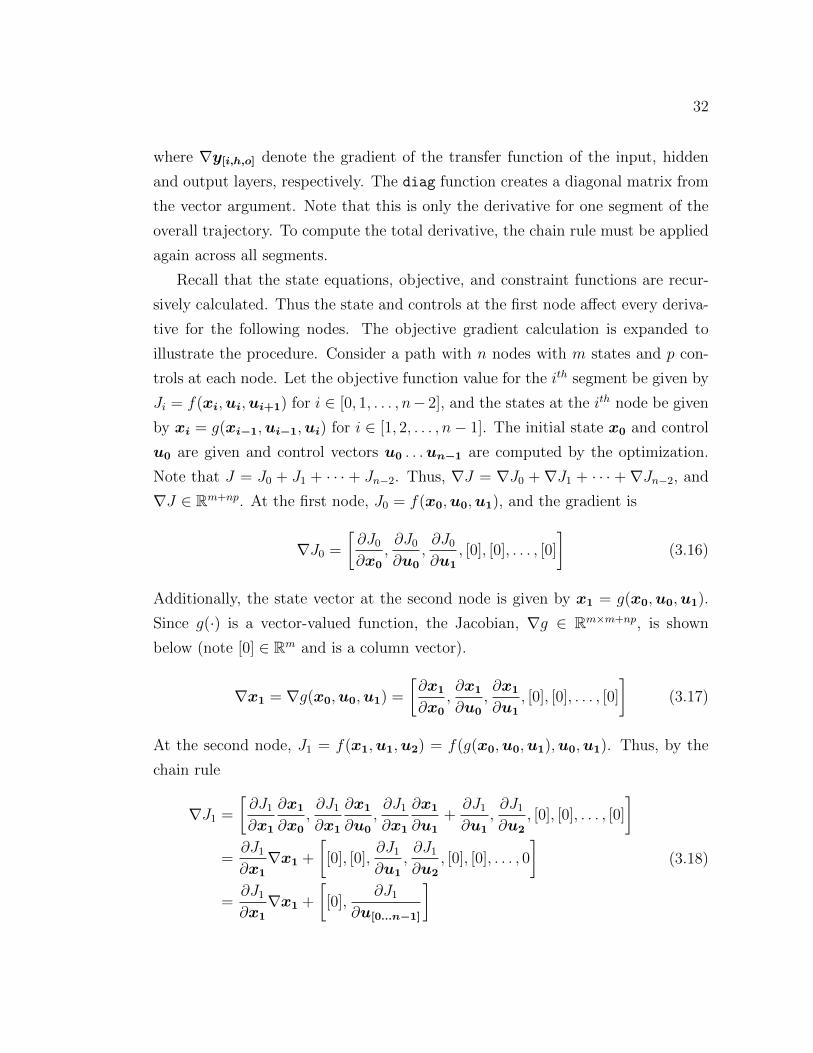
Note that J = J0 + J1 + ⋅ ⋅ ⋅ + Jn−2. Thus, ∇J = ∇J0 +∇J1 + ⋅ ⋅ ⋅ +∇Jn−2, and
∇J ∈ ℝm+np. At the first node, J0 = f(x0,u0,u1), and the gradient is
∇J0 =
[∂J0∂x0
,∂J0∂u0
,∂J0∂u1
, [0], [0], . . . , [0]
](3.16)
Additionally, the state vector at the second node is given by x1 = g(x0,u0,u1).
Since g(⋅) is a vector-valued function, the Jacobian, ∇g ∈ ℝm×m+np, is shown
below (note [0] ∈ ℝm and is a column vector).
∇x1 = ∇g(x0,u0,u1) =
[∂x1
∂x0
,∂x1
∂u0
,∂x1
∂u1
, [0], [0], . . . , [0]
](3.17)
At the second node, J1 = f(x1,u1,u2) = f(g(x0,u0,u1),u0,u1). Thus, by the
chain rule
∇J1 =
[∂J1∂x1
∂x1
∂x0
,∂J1∂x1
∂x1
∂u0
,∂J1∂x1
∂x1
∂u1
+∂J1∂u1
,∂J1∂u2
, [0], [0], . . . , [0]
]=∂J1∂x1
∇x1 +
[[0], [0],
∂J1∂u1
,∂J1∂u2
, [0], [0], . . . , 0
]=∂J1∂x1
∇x1 +
[[0],
∂J1∂u[0...n−1]
] (3.18)

33
The state vector at the third node is given by
x2 = g(x1,u1,u2) = g(g(x0,u0,u1),u1,u2) (3.19)
Therefore, the Jacobian is
∇x2 =
[∂x2
∂x1
∂x1
∂x0
,∂x2
∂x1
∂x1
∂u0
,∂x2
∂x1
∂x1
∂u1
+∂x2
∂u1
,∂x2
∂u2
, [0], [0], . . . , [0]
]=∂x2
∂x1
∇x1 +
[[0], [0],
∂x2
∂u1
,∂x2
∂u2
, [0], [0], . . . , [0]
]=∂x2
∂x1
∇x1 +
[[0],
∂x2
∂u[0...n−1]
] (3.20)
The remaining segments are iterated over in similar fashion. Recursively, the
derivative computation is given by
∇x0 =[Im×m [0]m×np] (3.21a)
∇J = ∇J +∂Ji∂xi
∇xi−1 +
[[0],
∂Ji∂u[0...n−1]
](3.21b)
∇xi =∂xi
∂xi−1
∇xi−1 +
[[0],
∂xi
∂u[0...n−1]
](3.21c)
In the final result, the first m + p columns are not used because these are the
derivatives with respect to x0 and u0 which remain constant.
It is also convenient to extract out the state constraint derivatives as needed
during iteration over the segments. The affected rows of the state constraint Ja-
cobian at the itℎ segment are given by
ksc = [1 : nlim] + nlimi (3.22)
where nlim is the number of states subject to constraints. The vector k contains
the indices of the states that are subject to a constraint. At each segment, the
rows in the state constraint Jacobian identified in Equation 3.22 are computed.
∇C(ksc) = ∇xi(k) (3.23)
34
In words, Equation 3.23 states that the affected rows (k) of the states Jacobian for
the itℎ segment are put into the affected rows (ksc) of the state constraint Jacobian.
For example, if a constraint is placed on the third state of a system, the third row
of ∇xi would be placed in the itℎ row of C. Note that while the constraints on
the state are simple limits, nonlinear constraints are necessary because the states
are not part of the varied parameters (only the controls are) and are nonlinear
functions of the control input. While no other general constraints were imposed in
this problem, they are simple to add and would follow the implementation of the
objective function.
3.5 Training
Typical neural network training methods are used. The state and control limits
are defined and a set of random points within these limits is used as training
data. If possible, the training data should use relative values (such as the relative
distance from a UAV to a target) to reduce the size of the function space. Given
a random initial state and random initial and final controls, the state equations
are integrated over the timestep using a linearly interpolated control time history.
If the resulting states are within limits, the state vector is saved. If the resulting
states are out of bounds, new initial state and initial and final control vectors are
generated.
More details on the training procedure are given in the following chapter. The
neural network approximation method is applied to UAV surveillance problem
described in the following chapter. It is compared with the direct collocation and
psuedospectral methods in terms of trajectory results and computation time.
Chapter 4UAV Path Planning Surveillance
Problem
In this chapter, a UAV surveillance problem is described as a non-trival application
of the direct collocation, pseudospectral, and neural network approximation meth-
ods. The problem is stated as follows: given one or more UAVs, a fixed, onboard
camera whose intrinsic parameters are known, and a ground target whose location
is estimated from onboard sensors, maximize surveillance time while observing the
performance limits of the aircraft and accounting for external disturbances such
as wind or target motion. Simulation results produced in Matlab are presented in
this chapter; in the following chapter, flight testing of the algorithm in real time
onboard a UAV is discussed.
4.1 Equations of Motion
The problem is approached with a reduced set of equations of motion for the UAV
and target. Motion in only two dimensions is assumed, keeping altitude constant.
Let xu be the state vector of an aircraft, xt be the state vector of a target, and
u be the aircraft control vector. For the simplified dynamic model, the states are
are North and East position of the UAV and target (x, y, xt, yt), airspeed of the
UAV (Vt), and heading of the UAV ( ). The controls are longitudinal acceleration

36
command (ua) and bank angle command (u�).
xu =
⎡⎢⎢⎢⎢⎣x
y
Vt
⎤⎥⎥⎥⎥⎦ u =
[ua
u�
]xt =
[xt
yt
](4.1)
(4.2)
The complete dynamic model is given below for one aircraft and one target. The
aircraft equations account for a constant wind speed.
x = xu1 = Vt cos( )− VwindNy = xu2 = Vt sin( )− VwindEVt = xu3 = ua
= xu4 = g tan(u�)/Vt
xt = xt1 = VtgtN
yt = xt2 = VtgtE
(4.3)
Constraints on the problem include minimum and maximum airspeed, bank angle
limits, and longitudinal acceleration limits.
Vstall < Vt < Vmax
−�max < u� < �max
−amax < ua < amax
(4.4)
4.2 Discretization Scheme
When the continuous problem is transcribed into a nonlinear programming prob-
lem, the states and controls at each node are solved for. The vector containing all
of these values is called the parameter vector. As discussed previously, a receding
horizon approach is used. To apply any of the direct methods, the horizon time is
discretized with a number of nodes. The specific discretization differs between the
direct collocation/pseudospectral methods and the neural network method.
37
4.2.1 Direct Collocation and Pseudospectral Parameteri-
zation
The direct collocation and pseudospectral methods solve for both the states and
controls at each node. Let ps be the vector of all the states of all n UAVs and q
targets at a single node, and let pc be the vector of all n control vectors (for n
UAVs) at a single node (targets do not have control inputs):
ps =
⎡⎢⎢⎢⎢⎢⎢⎢⎢⎢⎢⎢⎢⎢⎢⎢⎢⎢⎢⎢⎢⎣
xu[0]
xu[1]
...
xu[n−2]
xu[n−1]
xt[0]
xt[1]
...
xt[q−2]
xt[q−1]
⎤⎥⎥⎥⎥⎥⎥⎥⎥⎥⎥⎥⎥⎥⎥⎥⎥⎥⎥⎥⎥⎦
pc =
⎡⎢⎢⎢⎢⎢⎢⎢⎣
u[0]
u[1]
...
u[n−2]
u[n−1]
⎤⎥⎥⎥⎥⎥⎥⎥⎦(4.5)
Now the problem matrix Pm is assembled for N node points:
Pm =
[ps0
ps1. . . psN−2
psN−1
pc0pc1
. . . pcN−2pcN−2
](4.6)
The states are organized in the matrix such that each row contains the values of a
single (particular) state at each node point; each column represents a node. The
nonlinear solver expects a single column vector. The problem matrix is reshaped
column-wise with the state vector row. The control vector row is reshaped column-
wise and appended to the state vector column.
4.2.2 Neural Network Approximation Parameterization
The neural network approximation does not solve for the states at each node, only
the controls. Therefore, only the controls section of the above parameter vector is
used in the nonlinear program.
38
4.3 Constraints
The complete list of problem constraints specific to the above formulation is given
in Equation 4.7. The defects Δ are constrained to zero. Note that the initial state
and controls (x0, u0) are the state and controls of the UAV and target at the time
the optimization is started and remain constant for the optimization. Through
the use of constraints on the bank angle command (u�), turn rate can be limited.
Similarly, longitudinal acceleration is limited by the constraint on ua.
Δ = 0
x0 = x0
u0 = u0
Vmin ≤ Vti ≤ Vmax
uamin ≤ uai ≤ uamax
u�min ≤ u�i ≤ u�max
(4.7)
When the path planner is started, an initial guess for the path over the horizon
is required. Since the direct collocation and pseudospectral methods require no
specific initial guess to converge, the current heading and speed of the UAV is
used to extrapolate a straight path out to the end of the horizon time.
The neural network method is slightly different. Because only the controls are
solved for in the nonlinear program, any state constraints must be added separately.
The airspeed limits are the only state constraints for this particular problem. State
constraints take the form of a constrained nonlinear function of the controls (the
approximated dynamics).
4.4 Objective Function
The desired behavior for the UAV is to maximize sensor coverage of the target.
The objective function that drives this behavior is a weighted sum of four separate
objectives.
J =
∫ tf
to
[w1u
2a + w2u
2� + w3((x− xt)2 + (y − yt)2) + w4Jtiv
](4.8)
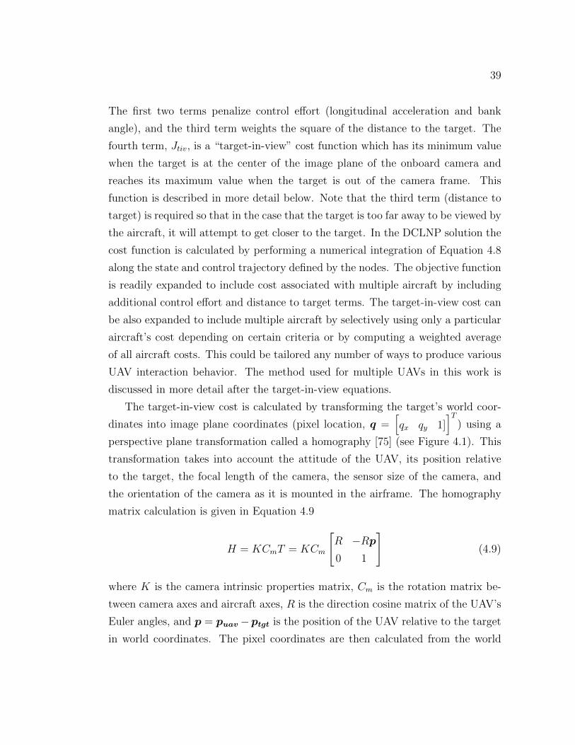
39
The first two terms penalize control effort (longitudinal acceleration and bank
angle), and the third term weights the square of the distance to the target. The
fourth term, Jtiv, is a “target-in-view” cost function which has its minimum value
when the target is at the center of the image plane of the onboard camera and
reaches its maximum value when the target is out of the camera frame. This
function is described in more detail below. Note that the third term (distance to
target) is required so that in the case that the target is too far away to be viewed by
the aircraft, it will attempt to get closer to the target. In the DCLNP solution the
cost function is calculated by performing a numerical integration of Equation 4.8
along the state and control trajectory defined by the nodes. The objective function
is readily expanded to include cost associated with multiple aircraft by including
additional control effort and distance to target terms. The target-in-view cost can
be also expanded to include multiple aircraft by selectively using only a particular
aircraft’s cost depending on certain criteria or by computing a weighted average
of all aircraft costs. This could be tailored any number of ways to produce various
UAV interaction behavior. The method used for multiple UAVs in this work is
discussed in more detail after the target-in-view equations.
The target-in-view cost is calculated by transforming the target’s world coor-
dinates into image plane coordinates (pixel location, q =[qx qy 1]
]T) using a
perspective plane transformation called a homography [75] (see Figure 4.1). This
transformation takes into account the attitude of the UAV, its position relative
to the target, the focal length of the camera, the sensor size of the camera, and
the orientation of the camera as it is mounted in the airframe. The homography
matrix calculation is given in Equation 4.9
H = KCmT = KCm
[R −Rp0 1
](4.9)
where K is the camera intrinsic properties matrix, Cm is the rotation matrix be-
tween camera axes and aircraft axes, R is the direction cosine matrix of the UAV’s
Euler angles, and p = puav−ptgt is the position of the UAV relative to the target
in world coordinates. The pixel coordinates are then calculated from the world
40
coordinates in Equation 4.10.
q = H[pT 1
]T(4.10)
The z-element of q must equal one:
q = (1/qz)[qx qy
]T(4.11)
This calculation can be simplified by removing the Z-coordinate column from R
in the top left corner of T because the model uses 2-dimensional motion at a fixed
altitude. In this formulation only the roll and yaw attitudes of the aircraft are
accounted for, further simplifying the calculation above. Pitch attitude is assumed
to be zero, but the effect of pitch could readily be added if more detailed equations
of motion are used. The camera orientation relative to the airframe is also assumed
to be constant. However, different camera installation orientations or a gimbaled
camera can be accounted for by a time dependent Cm matrix. The target-in-view
Target
Figure 4.1. Axes used in the homography
cost is zero if the target is in the center of the image and varies parabolically to
the edge of the image where its reaches its maximum value of one. Outside of the
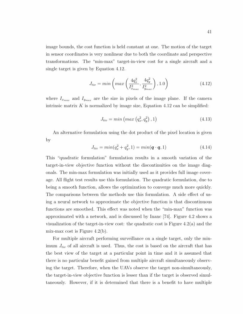
41
image bounds, the cost function is held constant at one. The motion of the target
in sensor coordinates is very nonlinear due to both the coordinate and perspective
transformations. The “min-max” target-in-view cost for a single aircraft and a
single target is given by Equation 4.12.
Jtiv = min
(max
(4q2xI2xmax
,4q2yI2ymax
), 1.0
)(4.12)
where Ixmax and Iymax are the size in pixels of the image plane. If the camera
intrinsic matrix K is normalized by image size, Equation 4.12 can be simplified:
Jtiv = min(max
(q2x, q
2y
), 1)
(4.13)
An alternative formulation using the dot product of the pixel location is given
by
Jtiv = min(q2x + q2y , 1) = min(q ⋅ q, 1) (4.14)
This “quadratic formulation” formulation results in a smooth variation of the
target-in-view objective function without the discontinuities on the image diag-
onals. The min-max formulation was initially used as it provides full image cover-
age. All flight test results use this formulation. The quadratic formulation, due to
being a smooth function, allows the optimization to converge much more quickly.
The comparisons between the methods use this formulation. A side effect of us-
ing a neural network to approximate the objective function is that discontinuous
functions are smoothed. This effect was noted when the “min-max” function was
approximated with a network, and is discussed by Inanc [74]. Figure 4.2 shows a
visualization of the target-in-view cost: the quadratic cost is Figure 4.2(a) and the
mix-max cost is Figure 4.2(b).
For multiple aircraft performing surveillance on a single target, only the min-
imum Jtiv of all aircraft is used. Thus, the cost is based on the aircraft that has
the best view of the target at a particular point in time and it is assumed that
there is no particular benefit gained from multiple aircraft simultaneously observ-
ing the target. Therefore, when the UAVs observe the target non-simultaneously,
the target-in-view objective function is lesser than if the target is observed simul-
taneously. However, if it is determined that there is a benefit to have multiple

42
-1 -0.5 0 0.5 1-1
-0.8
-0.6
-0.4
-0.2
0
0.2
0.4
0.6
0.8
1
0.8
0.6
0.40.2
1
0
1 1
1
0.1
(a) min(pTp, 1)
-1 -0.5 0 0.5 1-1
-0.8
-0.6
-0.4
-0.2
0
0.2
0.4
0.6
0.8
1
0.8
0.6
0.4
0.2
1
0
1 1
1
0.1
(b) min(max(x2s, y2s), 1)
Figure 4.2. Target-in-view cost functions
simultaneous observations, a weighted sum of all target-in-view-costs would pro-
duce this behavior.
Name Description Rationale
ControlEffort
Control input squaredAdjust magnitude ofcontrol response
Distance-to-target
Distance squared from the UAV totarget
Drive the UAV to-wards the target
Target-in-view
Target location transformed to pixelcoordinates; maximum value whenpixel coordinates exceed the imageboundaries, minimum value at thecenter of the image
Shape the path so thatviews of the target arecaptured
Table 4.1. Objective Function Listing
As a final overview of the entire process, the problem is parameterized by the
method in Section 4.2. The problem is then solved by searching for the parameter
vector (transformed form of Equation 4.6) that minimizes the objective function
(Equation 4.12) subject to the constraints (Equations. 2.9 & 4.7). The various
objective functions used are summarized in Table 4.1.
43
4.4.1 Integrating External World Data
The initial work for the path planner algorithm resulted from fairly simple re-
quirements: create a path such that the time spent with the sensor on the target is
maximized. However, by expanding the requirements, the planner becomes more
useful. One such way to increase capability of the planner is to include external
information of the surrounding area (e.g. roads). With the use of known roads,
the planner becomes less reliant on observations of target motion to be able to
predict future positions. For example, if the path planner has road data for the
area it is observing, it may be reasonable to assume a vehicle will follow the road
it is on, and therefore, the path planner already knows the path the vehicle will
most likely take. With this information, the path planner has access to a more
complete model of where a vehicle might go. As shown in Figure 4.3, estimates
of target speed, V , and position, s, along the road are used to make a prediction.
Since the vehicle’s motion is 1-dimensional along a road, the equation of motion is
simply
s = V (4.15)
The vehicle’s location is given by
[xt, yt] = f(s) (4.16)
The formulation of the trajectory optimization allows the use of any kind of
Figure 4.3. Path data illustration
predictive target motion model without modification to the underlying problem
parameterization. Simulation results using this feature are given in Section 4.6.
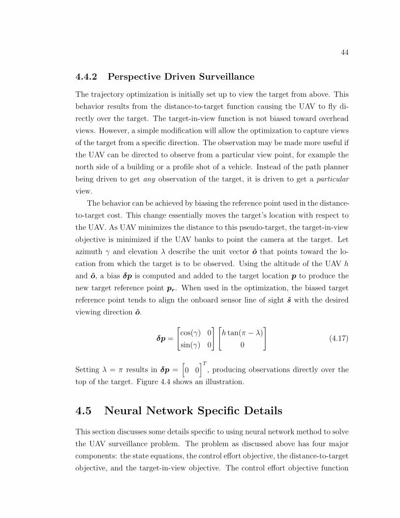
44
4.4.2 Perspective Driven Surveillance
The trajectory optimization is initially set up to view the target from above. This
behavior results from the distance-to-target function causing the UAV to fly di-
rectly over the target. The target-in-view function is not biased toward overhead
views. However, a simple modification will allow the optimization to capture views
of the target from a specific direction. The observation may be made more useful if
the UAV can be directed to observe from a particular view point, for example the
north side of a building or a profile shot of a vehicle. Instead of the path planner
being driven to get any observation of the target, it is driven to get a particular
view.
The behavior can be achieved by biasing the reference point used in the distance-
to-target cost. This change essentially moves the target’s location with respect to
the UAV. As UAV minimizes the distance to this pseudo-target, the target-in-view
objective is minimized if the UAV banks to point the camera at the target. Let
azimuth and elevation � describe the unit vector o that points toward the lo-
cation from which the target is to be observed. Using the altitude of the UAV ℎ
and o, a bias �p is computed and added to the target location p to produce the
new target reference point pr. When used in the optimization, the biased target
reference point tends to align the onboard sensor line of sight s with the desired
viewing direction o.
�p =
[cos( ) 0
sin( ) 0
][ℎ tan(� − �)
0
](4.17)
Setting � = � results in �p =[0 0
]T, producing observations directly over the
top of the target. Figure 4.4 shows an illustration.
4.5 Neural Network Specific Details
This section discusses some details specific to using neural network method to solve
the UAV surveillance problem. The problem as discussed above has four major
components: the state equations, the control effort objective, the distance-to-target
objective, and the target-in-view objective. The control effort objective function

45
N
E
os
d
Figure 4.4. Illustration of the perspective driven objective function
is kept as an analytical expression because it is very simple - expressions for its
derivative are easily written. The remaining three components are approximated
with feed-forward neural networks. However, the exact structure of the problem is
not used. Instead of separate states for the UAV and target locations, the relative
distance from the UAV to the target is used to reduce the dimension of the function
approximated by the neural network. This also reduces the required range of the
positional states since for relative distances over a certain magnitude the only
option is to fly toward the target. For this specific problem, relative distance to
the target was limited to ±1000ft. Limits were also applied to airspeed, bank
angle, and longitudinal acceleration corresponding to aircraft performance limits.
The input to the dynamics network is [Vt, , ua0 , u�0 , ua1 , u�1 ]T . Its output is
[�x, �y, Vt, ]T where �x and �y are change in position from the point corresponding
to the input data. The input for the distance-to-target and target-in-view functions
is [xrel, yrel, Vt, , ua0 , u�0 , ua1 , u�1 ]T . Output is a scalar value that approximates
the objectives. The networks used for the UAV surveillance problem are shown
schematically in Figure 4.5.
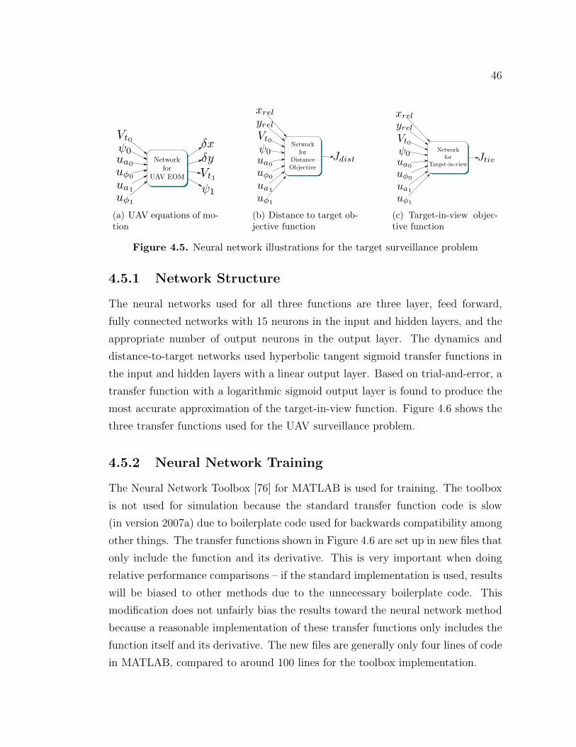
46
(a) UAV equations of mo-tion
(b) Distance to target ob-jective function
(c) Target-in-view objec-tive function
Figure 4.5. Neural network illustrations for the target surveillance problem
4.5.1 Network Structure
The neural networks used for all three functions are three layer, feed forward,
fully connected networks with 15 neurons in the input and hidden layers, and the
appropriate number of output neurons in the output layer. The dynamics and
distance-to-target networks used hyperbolic tangent sigmoid transfer functions in
the input and hidden layers with a linear output layer. Based on trial-and-error, a
transfer function with a logarithmic sigmoid output layer is found to produce the
most accurate approximation of the target-in-view function. Figure 4.6 shows the
three transfer functions used for the UAV surveillance problem.
4.5.2 Neural Network Training
The Neural Network Toolbox [76] for MATLAB is used for training. The toolbox
is not used for simulation because the standard transfer function code is slow
(in version 2007a) due to boilerplate code used for backwards compatibility among
other things. The transfer functions shown in Figure 4.6 are set up in new files that
only include the function and its derivative. This is very important when doing
relative performance comparisons – if the standard implementation is used, results
will be biased to other methods due to the unnecessary boilerplate code. This
modification does not unfairly bias the results toward the neural network method
because a reasonable implementation of these transfer functions only includes the
function itself and its derivative. The new files are generally only four lines of code
in MATLAB, compared to around 100 lines for the toolbox implementation.
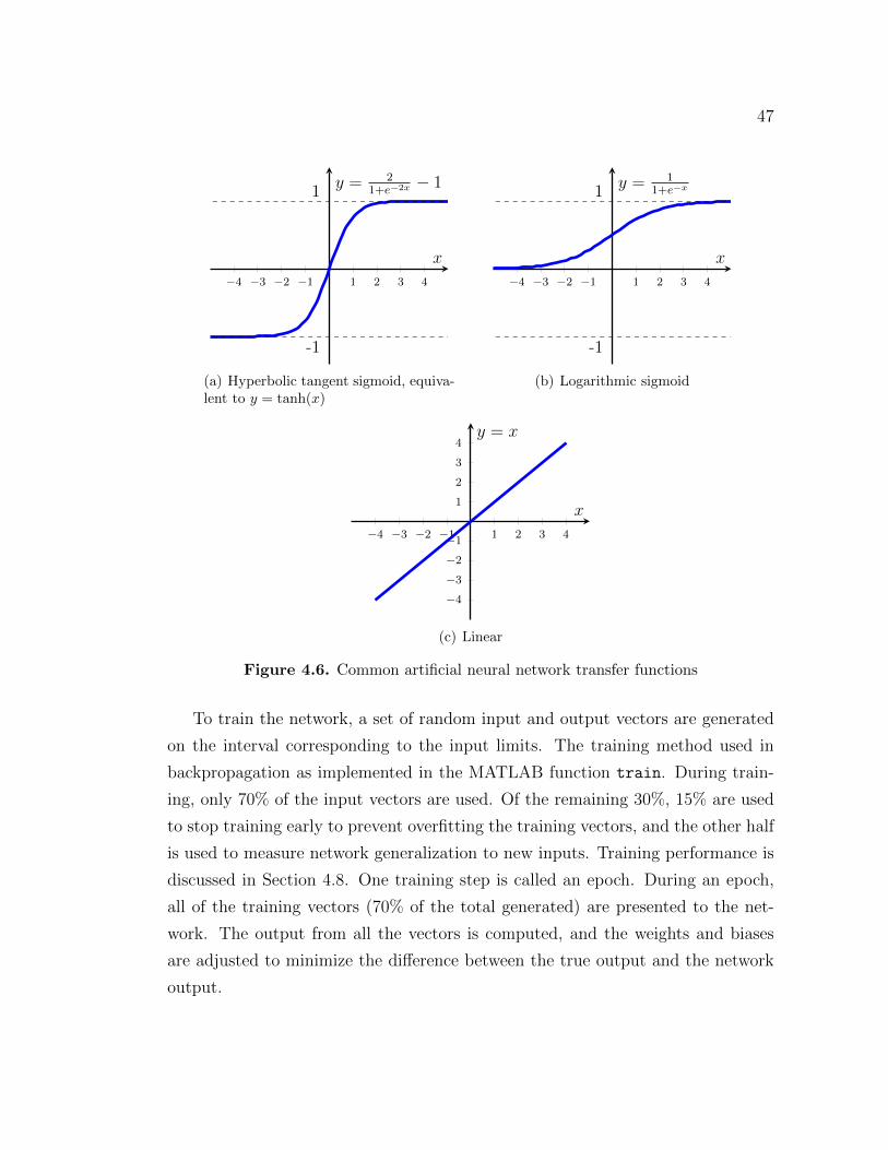
47
−4 −3 −2 −1 1 2 3 4
-1
1
x
y = 21+e−2x − 1
(a) Hyperbolic tangent sigmoid, equiva-lent to y = tanh(x)
−4 −3 −2 −1 1 2 3 4
-1
1
x
y = 11+e−x
(b) Logarithmic sigmoid
−4 −3 −2 −1 1 2 3 4
−4
−3
−2
−1
1
2
3
4
x
y = x
(c) Linear
Figure 4.6. Common artificial neural network transfer functions
To train the network, a set of random input and output vectors are generated
on the interval corresponding to the input limits. The training method used in
backpropagation as implemented in the MATLAB function train. During train-
ing, only 70% of the input vectors are used. Of the remaining 30%, 15% are used
to stop training early to prevent overfitting the training vectors, and the other half
is used to measure network generalization to new inputs. Training performance is
discussed in Section 4.8. One training step is called an epoch. During an epoch,
all of the training vectors (70% of the total generated) are presented to the net-
work. The output from all the vectors is computed, and the weights and biases
are adjusted to minimize the difference between the true output and the network
output.
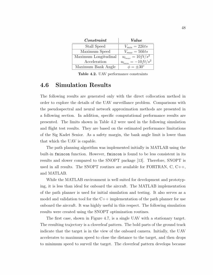
48
Constraint Value
Stall Speed Vmin = 22ktsMaximum Speed Vmax = 50kts
Maximum Longitudinal ulmax = 10ft/s2
Acceleration ulmin = −10ft/s2
Maximum Bank Angle � = ±30∘
Table 4.2. UAV performance constraints
4.6 Simulation Results
The following results are generated only with the direct collocation method in
order to explore the details of the UAV surveillance problem. Comparisons with
the pseudospectral and neural network approximation methods are presented in
a following section. In addition, specific computational performance results are
presented. The limits shown in Table 4.2 were used in the following simulation
and flight test results. They are based on the estimated performance limitations
of the Sig Kadet Senior. As a safety margin, the bank angle limit is lower than
that which the UAV is capable.
The path planning algorithm was implemented initially in MATLAB using the
built-in fmincon function. However, fmincon is found to be less consistent in its
results and slower compared to the SNOPT package [13]. Therefore, SNOPT is
used in all results. The SNOPT routines are available for FORTRAN, C, C++,
and MATLAB.
While the MATLAB environment is well suited for development and prototyp-
ing, it is less than ideal for onboard the aircraft. The MATLAB implementation
of the path planner is used for initial simulation and testing. It also serves as a
model and validation tool for the C++ implementation of the path planner for use
onboard the aircraft. It was highly useful in this respect. The following simulation
results were created using the SNOPT optimization routines.
The first case, shown in Figure 4.7, is a single UAV with a stationary target.
The resulting trajectory is a cloverleaf pattern. The bold parts of the ground track
indicate that the target is in the view of the onboard camera. Initially, the UAV
accelerates to maximum speed to close the distance to the target, and then drops
to minimum speed to surveil the target. The cloverleaf pattern develops because
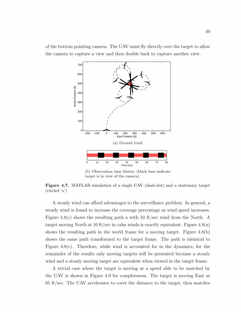
49
of the bottom pointing camera. The UAV must fly directly over the target to allow
the camera to capture a view and then double back to capture another view.
−200 −100 0 100 200 300 400 500 6000
100
200
300
400
500
600
700
Nor
th P
ositi
on (
ft)
East Position (ft)
(a) Ground track
0 10 20 30 40 50 60 70 80Time (sec)
(b) Observation time history (black bars indicatetarget is in view of the camera)
Figure 4.7. MATLAB simulation of a single UAV (dash-dot) and a stationary target(circled ‘x’)
A steady wind can afford advantages to the surveillance problem. In general, a
steady wind is found to increase the coverage percentage as wind speed increases.
Figure 4.8(c) shows the resulting path a with 10 ft/sec wind from the North. A
target moving North at 10 ft/sec in calm winds is exactly equivalent. Figure 4.8(a)
shows the resulting path in the world frame for a moving target. Figure 4.8(b)
shows the same path transformed to the target frame. The path is identical to
Figure 4.8(c). Therefore, while wind is accounted for in the dynamics, for the
remainder of the results only moving targets will be presented because a steady
wind and a steady moving target are equivalent when viewed in the target frame.
A trivial case where the target is moving at a speed able to be matched by
the UAV is shown in Figure 4.9 for completeness. The target is moving East at
65 ft/sec. The UAV accelerates to cover the distance to the target, then matches
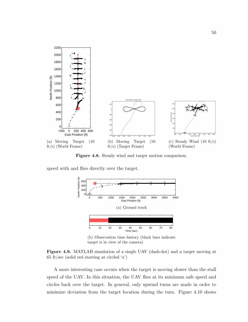
50
−200 0 200 400 6000
200
400
600
800
1000
1200
1400
1600
1800
2000
2200N
orth
Pos
ition
(ft)
East Position (ft)
(a) Moving Target (10ft/s) (World Frame)
−400 −300 −200 −100 0 100 200 300−500
−400
−300
−200
−100
0
100
UAV Motion in target frame
(b) Moving Target (10ft/s) (Target Frame)
−200 −100 0 100 200 300 400 500 6000
100
200
300
400
500
600
Nor
th P
ositi
on (
ft)
East Position (ft)
(c) Steady Wind (10 ft/s)(World Frame)
Figure 4.8. Steady wind and target motion comparison.
speed with and flies directly over the target.
0 500 1000 1500 2000 2500 3000 3500 40000
200
400
600
Nor
th P
ositi
on (
ft)
East Position (ft)
(a) Ground track
0 10 20 30 40 50 60 70 80Time (sec)
(b) Observation time history (black bars indicatetarget is in view of the camera)
Figure 4.9. MATLAB simulation of a single UAV (dash-dot) and a target moving at65 ft/sec (solid red starting at circled ‘x’)
A more interesting case occurs when the target is moving slower than the stall
speed of the UAV. In this situation, the UAV flies at its minimum safe speed and
circles back over the target. In general, only upwind turns are made in order to
minimize deviation from the target location during the turn. Figure 4.10 shows
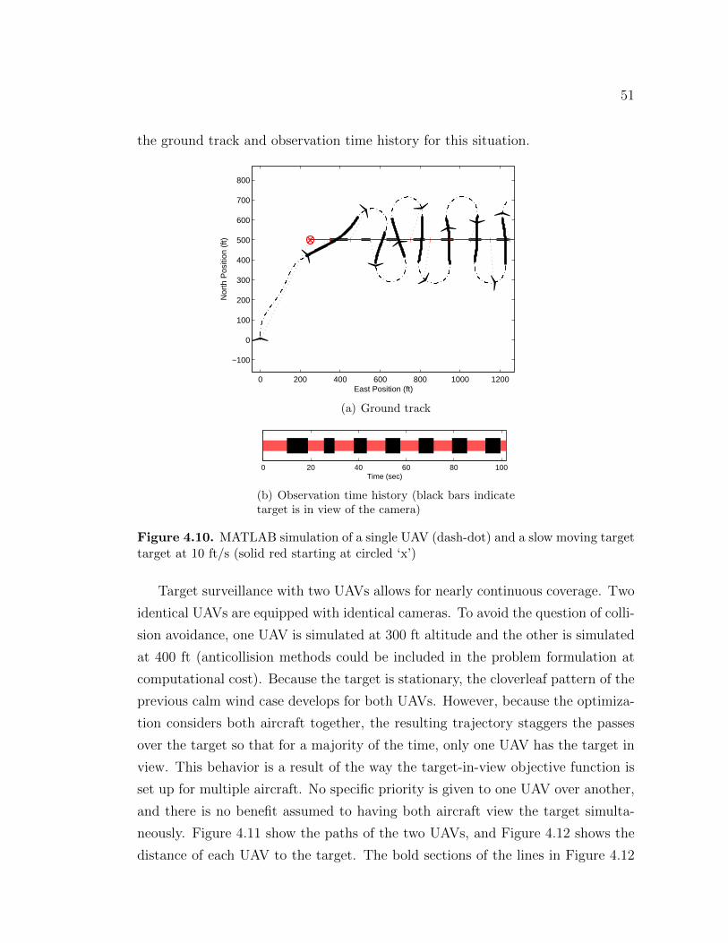
51
the ground track and observation time history for this situation.
0 200 400 600 800 1000 1200
−100
0
100
200
300
400
500
600
700
800
Nor
th P
ositi
on (
ft)
East Position (ft)
(a) Ground track
0 20 40 60 80 100Time (sec)
(b) Observation time history (black bars indicatetarget is in view of the camera)
Figure 4.10. MATLAB simulation of a single UAV (dash-dot) and a slow moving targettarget at 10 ft/s (solid red starting at circled ‘x’)
Target surveillance with two UAVs allows for nearly continuous coverage. Two
identical UAVs are equipped with identical cameras. To avoid the question of colli-
sion avoidance, one UAV is simulated at 300 ft altitude and the other is simulated
at 400 ft (anticollision methods could be included in the problem formulation at
computational cost). Because the target is stationary, the cloverleaf pattern of the
previous calm wind case develops for both UAVs. However, because the optimiza-
tion considers both aircraft together, the resulting trajectory staggers the passes
over the target so that for a majority of the time, only one UAV has the target in
view. This behavior is a result of the way the target-in-view objective function is
set up for multiple aircraft. No specific priority is given to one UAV over another,
and there is no benefit assumed to having both aircraft view the target simulta-
neously. Figure 4.11 show the paths of the two UAVs, and Figure 4.12 shows the
distance of each UAV to the target. The bold sections of the lines in Figure 4.12
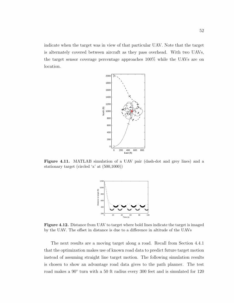
52
indicate when the target was in view of that particular UAV. Note that the target
is alternately covered between aircraft as they pass overhead. With two UAVs,
the target sensor coverage percentage approaches 100% while the UAVs are on
location.
0 200 400 600 800
0
200
400
600
800
1000
1200
1400
1600
1800
2000
East (ft)
Nor
th (
ft)
Figure 4.11. MATLAB simulation of a UAV pair (dash-dot and grey lines) and astationary target (circled ‘x’ at (500,1000))
0 20 40 60 80 100200
400
600
800
1000
1200
Time (s)
Dis
tanc
e to
targ
et (
ft)
Figure 4.12. Distance from UAV to target where bold lines indicate the target is imagedby the UAV. The offset in distance is due to a difference in altitude of the UAVs
The next results are a moving target along a road. Recall from Section 4.4.1
that the optimization makes use of known road data to predict future target motion
instead of assuming straight line target motion. The following simulation results
is chosen to show an advantage road data gives to the path planner. The test
road makes a 90∘ turn with a 50 ft radius every 300 feet and is simulated for 120

53
seconds. The path generated is shown below in Figure 4.13(a). The solid red
line represents the target’s path along the road, and the black dash-dot line is the
UAV’s path. In this case, the speed of the target was within the speed range of
the UAV. The target is in view of the UAV’s camera 88% of the time, as seen
in Figure 4.13(b). An interesting situation occurs when the vehicle is capable of
0 500 1000 1500 2000 25000
200
400
600
800
1000
Nor
th P
ositi
on (
ft)
East Position (ft)
(a) Ground track
0 20 40 60 80 100 120Time (sec)
(b) Observation time history (black bars indicatetarget is in view of the camera)
Figure 4.13. Path planner simulation with road data, target slower than max UAVspeed
traveling faster than the UAV, but the vehicle must use a curvy road. The path
planner accounts for this by following the target in a ‘looser’ fashion; making up for
the speed difference by taking advantage of the curves in the road. Figure 4.14(a)
illustrates this behavior. For this run, the target speed is set to 100 ft/sec while
the maximum UAV speed is 87 ft/sec. The path planner creates a path that cuts
across the curves in the road to make up for the speed difference. Even though
the target is moving faster than the UAV, the camera is viewing the target 100%
of the time because the UAV banks to keep it in view. With a gimbaled camera,
the banking would not be necessary.
Several perspective driven case are now shown. In the first case, the target is
stationary, and the UAV is to capture view of the north side from 400 ft altitude
at an elevation angle of 45∘. Figure 4.15 shows the ground track and observation
time history. In this case, the downward pointing camera is advantageous because
it points outward in a turn. The UAV is in a constant bank turn at its maximum
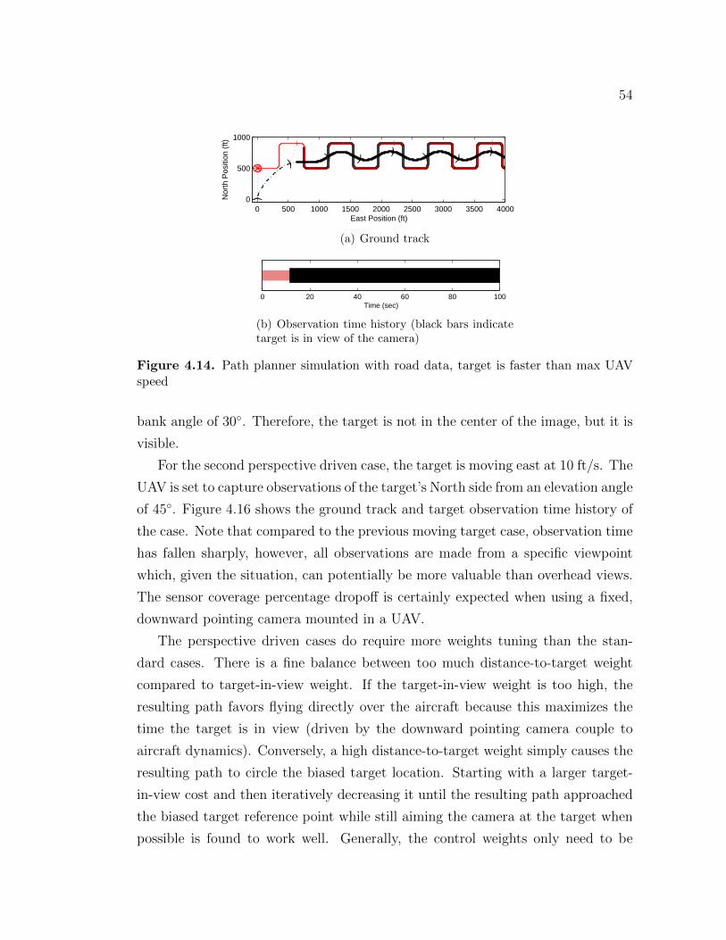
54
0 500 1000 1500 2000 2500 3000 3500 40000
500
1000
Nor
th P
ositi
on (
ft)East Position (ft)
(a) Ground track
0 20 40 60 80 100Time (sec)
(b) Observation time history (black bars indicatetarget is in view of the camera)
Figure 4.14. Path planner simulation with road data, target is faster than max UAVspeed
bank angle of 30∘. Therefore, the target is not in the center of the image, but it is
visible.
For the second perspective driven case, the target is moving east at 10 ft/s. The
UAV is set to capture observations of the target’s North side from an elevation angle
of 45∘. Figure 4.16 shows the ground track and target observation time history of
the case. Note that compared to the previous moving target case, observation time
has fallen sharply, however, all observations are made from a specific viewpoint
which, given the situation, can potentially be more valuable than overhead views.
The sensor coverage percentage dropoff is certainly expected when using a fixed,
downward pointing camera mounted in a UAV.
The perspective driven cases do require more weights tuning than the stan-
dard cases. There is a fine balance between too much distance-to-target weight
compared to target-in-view weight. If the target-in-view weight is too high, the
resulting path favors flying directly over the aircraft because this maximizes the
time the target is in view (driven by the downward pointing camera couple to
aircraft dynamics). Conversely, a high distance-to-target weight simply causes the
resulting path to circle the biased target location. Starting with a larger target-
in-view cost and then iteratively decreasing it until the resulting path approached
the biased target reference point while still aiming the camera at the target when
possible is found to work well. Generally, the control weights only need to be
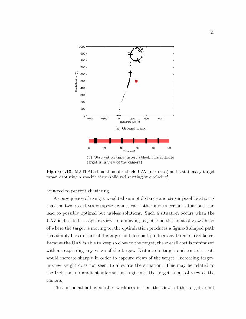
55
−400 −200 0 200 400 6000
100
200
300
400
500
600
700
800
900
1000
Nor
th P
ositi
on (
ft)
East Position (ft)
(a) Ground track
0 20 40 60 80 100Time (sec)
(b) Observation time history (black bars indicatetarget is in view of the camera)
Figure 4.15. MATLAB simulation of a single UAV (dash-dot) and a stationary targettarget capturing a specific view (solid red starting at circled ‘x’)
adjusted to prevent chattering.
A consequence of using a weighted sum of distance and sensor pixel location is
that the two objectives compete against each other and in certain situations, can
lead to possibly optimal but useless solutions. Such a situation occurs when the
UAV is directed to capture views of a moving target from the point of view ahead
of where the target is moving to, the optimization produces a figure-8 shaped path
that simply flies in front of the target and does not produce any target surveillance.
Because the UAV is able to keep so close to the target, the overall cost is minimized
without capturing any views of the target. Distance-to-target and controls costs
would increase sharply in order to capture views of the target. Increasing target-
in-view weight does not seem to alleviate the situation. This may be related to
the fact that no gradient information is given if the target is out of view of the
camera.
This formulation has another weakness in that the views of the target aren’t

56
0 200 400 600 800 1000 1200 1400 1600
0
200
400
600
800
1000
1200
Nor
th P
ositi
on (
ft)
East Position (ft)
(a) Ground track
0 20 40 60 80 100Time (sec)
(b) Observation time history (black bars indicatetarget is in view of the camera)
Figure 4.16. MATLAB simulation of a single UAV (dash-dot) and a slow moving targettarget capturing a specific view (solid red starting at circled ‘x’)
actually along a 45∘ angle, but are closer to 60∘. This is due to the fact that
none of the objective functions explicitly derive a cost number from the desired
alignment of the sensor line of sight and the desired observation line of sight.
Adding an additional objective that is minimum only when the sensor is pointing
at the target from the desired line of sight may help here.
Because the target-in-view function is held constant when the target is not
visible to the camera, no gradient information is available to the optimization. A
revised target-in-view objective with a small negative slope outside of the image
plane boundaries may perform better in perspective driven cases.
4.7 Convergence Results
Convergence of the above solutions is now discussed. Two different notions of con-
vergence are investigated: 1) convergence of the collocation method with increasing

57
number of nodes distributed over a constant horizon length and 2) receding horizon
convergence with increasing horizon length using constant node spacing in time.
For each case, the target observation ratio is computed. This ratio is the amount
of time the target is viewed by the onboard camera divided by the total maneuver
time. However, some care needs to be taken when calculating this number. As the
target falls in and out of view, this ratio will vary cyclically making the final result
dependent on when the maneuver ends. Therefore, running averages of different
window lengths are used. For these results, windows of 30, 60, and 120 seconds
are used. These windows generally cover several cycles of the behavior shown by
the path planner when observing targets in various situations. The final number is
an average of these three windowed averages. Figure 4.17 shows the time history
of the observation ratio for a single stationary target along with the windowed
averages.
0 50 100 150 2000
0.1
0.2
0.3
0.4
0.5
0.6
0.7
0.8
0.9
1
Obs
erva
tion
perc
enta
ge
Time (sec)
Mean of windowed means: 40.4%
Running mean30 sec window60 sec window120 sec windowMean of windowed means
Figure 4.17. Observation ratio time history with windowed averages for a stationarytarget
4.7.1 Discretization Convergence
In order to say the result of the collocation methods are optimal, their results
computed with an increasing number of nodes over a constant horizon length are
compared. Discretization convergence test results are presented here for target

58
speeds of 0, 10, 20, 25, 27, and 35 ft/sec. The uneven choice in speeds is used
because they generally represent uniform increases in the target observation time
ratio. Two horizon lengths are given, 16 and 30 seconds. For the 16 second
Number of NodesVtarg(ft/s) 9 18 36 72
0 40.4% 42.5% 43.2% 43.1%
Coverage
%
10 45.2% 47.4% 49.0% 50.3%20 53.9% 57.5% 55.6% 60.0%25 66.0% 72.2% 70.8% 72.3%27 73.6% 73.6% 77.6% 77.5%35 89.9% 94.3% 95.7% 96.7%
Table 4.3. Target coverage convergence using a 16 second horizon (mean of windowedmeans)
horizon (Table 4.3), the target coverage percentage increases by 5% to 11% as the
number of nodes are increased, depending on target speed. The percentage increase
also generally decreases as the number of nodes are doubled, which indicates the
collocation method does converge to a local minimum. However, there are some
anomalies. For Vtarg = 20ft/s, the observation ratio falls by 3% as the number of
nodes are doubled to 36 from 18. This can be explained by the difference in the
transient starting path between the two cases. Running both cases for a longer
simulation time reduces this difference. Such is the case for Vtarg = 27ft/s. When
Vtarg = 35ft/s, the UAV is able to surveil the target 100% of the time by slowly
rolling back and forth. When 9 nodes are used, the integration is not accurate
enough to produce this behavior. However, for 18 nodes and above, this behavior
is seen. Note that the observation ratio is not 100%, but would be if the maneuver
is allowed to continue indefinitely as the behavior requires around 120 seconds (in
all cases) to develop. With longer horizon length, the behavior develops much
more quickly.
The 30-second horizon case behaves similarly. However, for Vtarg = 25ft/s the
observation fraction decreases as the number of nodes are increased. This appears
to be related to how the numerical integration is computed. Ten intermediate
segments are used in the quadrature computation, regardless of how small node
spacing is. This may contribute to a spike in roll angle which the observation
ratio computation does not see, but the optimization does. For the case of Vtarg =
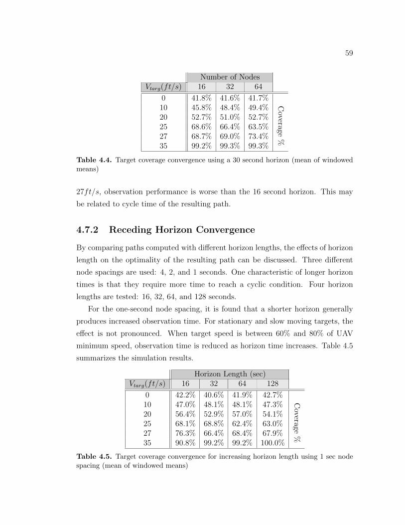
59
Number of NodesVtarg(ft/s) 16 32 64
0 41.8% 41.6% 41.7%
Coverage
%
10 45.8% 48.4% 49.4%20 52.7% 51.0% 52.7%25 68.6% 66.4% 63.5%27 68.7% 69.0% 73.4%35 99.2% 99.3% 99.3%
Table 4.4. Target coverage convergence using a 30 second horizon (mean of windowedmeans)
27ft/s, observation performance is worse than the 16 second horizon. This may
be related to cycle time of the resulting path.
4.7.2 Receding Horizon Convergence
By comparing paths computed with different horizon lengths, the effects of horizon
length on the optimality of the resulting path can be discussed. Three different
node spacings are used: 4, 2, and 1 seconds. One characteristic of longer horizon
times is that they require more time to reach a cyclic condition. Four horizon
lengths are tested: 16, 32, 64, and 128 seconds.
For the one-second node spacing, it is found that a shorter horizon generally
produces increased observation time. For stationary and slow moving targets, the
effect is not pronounced. When target speed is between 60% and 80% of UAV
minimum speed, observation time is reduced as horizon time increases. Table 4.5
summarizes the simulation results.
Horizon Length (sec)Vtarg(ft/s) 16 32 64 128
0 42.2% 40.6% 41.9% 42.7%
Coverage
%
10 47.0% 48.1% 48.1% 47.3%20 56.4% 52.9% 57.0% 54.1%25 68.1% 68.8% 62.4% 63.0%27 76.3% 66.4% 68.4% 67.9%35 90.8% 99.2% 99.2% 100.0%
Table 4.5. Target coverage convergence for increasing horizon length using 1 sec nodespacing (mean of windowed means)

60
For the two-second node spacing, similar behavior is observed.
Horizon Length (sec)Vtarg(ft/s) 16 32 64 128
0 40.4% 41.0% 44.3% 42.2%C
overage%
10 45.2% 45.3% 45.9% 45.2%20 53.9% 51.6% 54.3% 50.5%25 66.0% 69.3% 64.4% 61.0%27 73.6% 64.1% 67.7% 66.5%35 89.9% 99.2% 99.1% 100.0%
Table 4.6. Target coverage convergence for increasing horizon length using 2 sec nodespacing (mean of windowed means)
A node spacing of four seconds is shown in Table 4.7. At this node spacing,
the cubic Hermite approximation begins to break down. The polynomial approx-
imation is no longer able to accurately represent the dynamics of the UAV over
this length of time. However, the trend of increasing horizon time corresponding
to increased coverage percentage is clearly visible, though the percentage itself is
not as high compared to smaller node spacings. This reversal from the previous
cases is likely tied to the approximation accuracy reduction. While over short
time periods the path planner is not able to produce high observation time ratios,
a longer horizon may alleviate the approximation accuracy problem by possibly
time averaging the error.
Horizon Length (sec)Vtarg(ft/s) 16 32 64 128
0 35.5% 35.5% 36.6% 36.8%
Coverage
%
10 26.6% 32.0% 35.8% 37.0%20 38.3% 38.6% 44.1% 44.2%25 48.6% 58.9% 51.9% 53.2%27 46.2% 55.7% 57.3% 56.8%35 82.6% 99.3% 99.2% 99.2%
Table 4.7. Target coverage convergence for increasing horizon length using 4 sec nodespacing (mean of windowed means)
These results suggest that a shorter horizon length provides increased observa-
tion time if the target is mobile but slower than the UAV and the segment time
length is sufficiently small for acceptable approximation accuracy. The reason a

61
longer horizon reduces performance in this case may be that the chances of the
optimization stopping in a less optimal local minimum are increased with a longer
horizon time. In any case, the above tests provide evidence that shorter horizon
lengths can be used without loss in observation time. This is beneficial for real
time performance. In addition, it may be useful to vary the horizon length based
on target behavior. If a long segment time is required, it is beneficial to use a
longer horizon time to make up for increased approximation error.
4.8 Comparative Results
In this section, results are presented comparing the direct collocation, pseudospec-
tral, and neural network approximation methods.
4.8.1 Training
The dynamics network generally only required 5000 training samples to accurately
represent the true dynamics. The distance-to-target objective required 10000. The
target-in-view function is the most complex of the three since it involves a coordi-
nate rotation and perspective transform. While decent performance was obtained
with 15000 input vectors, 40000 input vectors greatly increased performance in
terms of the solution speed of the optimization solver. Figure 4.18 shows the cor-
respondence between scaled true output and scaled network output of each network
after training is complete. Note that only 70% of the total training set was used for
training. The remaining data is split evenly between validation and testing. The
validation data is used to stop network training early if the approximation error
increases. This ensures the network does not overfit the training data (the network
is highly accurate at the training points but has very poor accuracy on points it has
not be trained on). Test data is used to measure network generalization, or how
well the network performs on data it has not seen in training. Figure 4.18 shows
the complete, scaled training set. The network outputs are plotted against the true
outputs. Both the dynamics and distance-to-target networks’ plots are centered
on the line y = x, which shows these networks approximate their functions very
accurately. A large majority of the target-in-view output points are equal to one,
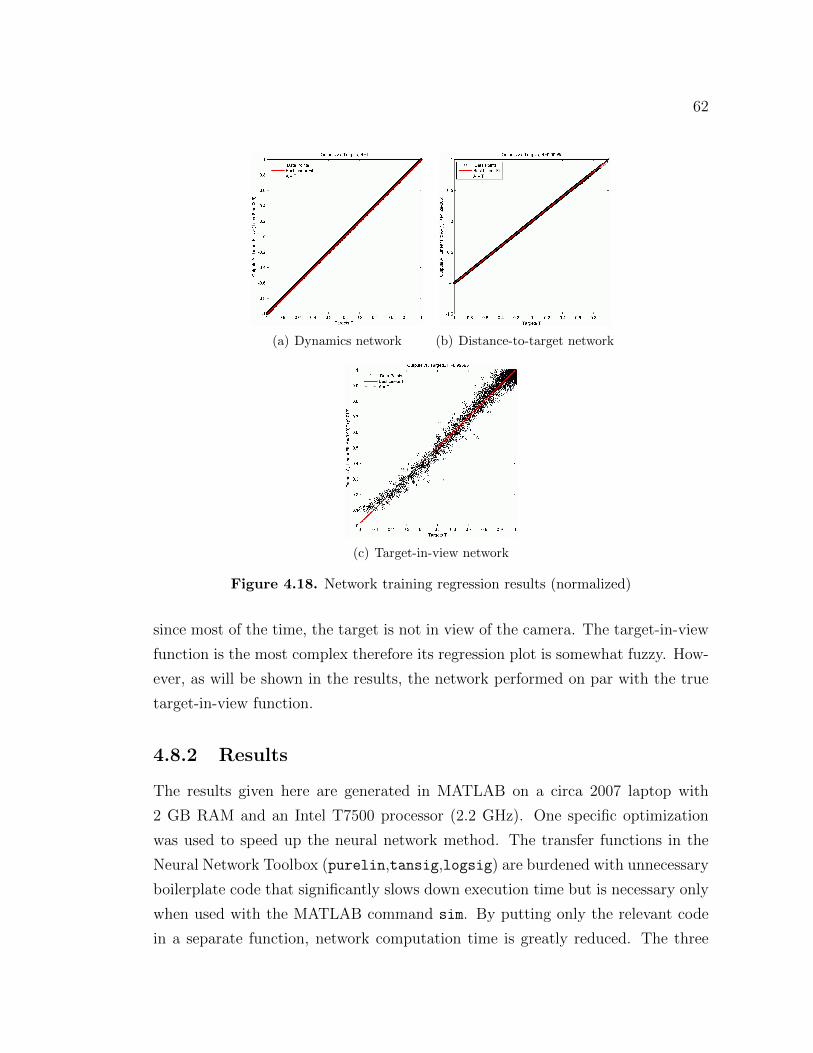
62
(a) Dynamics network (b) Distance-to-target network
(c) Target-in-view network
Figure 4.18. Network training regression results (normalized)
since most of the time, the target is not in view of the camera. The target-in-view
function is the most complex therefore its regression plot is somewhat fuzzy. How-
ever, as will be shown in the results, the network performed on par with the true
target-in-view function.
4.8.2 Results
The results given here are generated in MATLAB on a circa 2007 laptop with
2 GB RAM and an Intel T7500 processor (2.2 GHz). One specific optimization
was used to speed up the neural network method. The transfer functions in the
Neural Network Toolbox (purelin,tansig,logsig) are burdened with unnecessary
boilerplate code that significantly slows down execution time but is necessary only
when used with the MATLAB command sim. By putting only the relevant code
in a separate function, network computation time is greatly reduced. The three
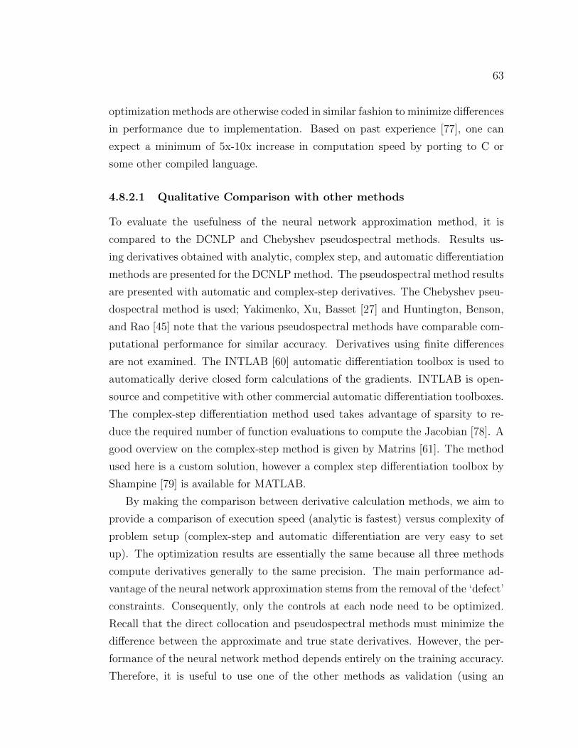
63
optimization methods are otherwise coded in similar fashion to minimize differences
in performance due to implementation. Based on past experience [77], one can
expect a minimum of 5x-10x increase in computation speed by porting to C or
some other compiled language.
4.8.2.1 Qualitative Comparison with other methods
To evaluate the usefulness of the neural network approximation method, it is
compared to the DCNLP and Chebyshev pseudospectral methods. Results us-
ing derivatives obtained with analytic, complex step, and automatic differentiation
methods are presented for the DCNLP method. The pseudospectral method results
are presented with automatic and complex-step derivatives. The Chebyshev pseu-
dospectral method is used; Yakimenko, Xu, Basset [27] and Huntington, Benson,
and Rao [45] note that the various pseudospectral methods have comparable com-
putational performance for similar accuracy. Derivatives using finite differences
are not examined. The INTLAB [60] automatic differentiation toolbox is used to
automatically derive closed form calculations of the gradients. INTLAB is open-
source and competitive with other commercial automatic differentiation toolboxes.
The complex-step differentiation method used takes advantage of sparsity to re-
duce the required number of function evaluations to compute the Jacobian [78]. A
good overview on the complex-step method is given by Matrins [61]. The method
used here is a custom solution, however a complex step differentiation toolbox by
Shampine [79] is available for MATLAB.
By making the comparison between derivative calculation methods, we aim to
provide a comparison of execution speed (analytic is fastest) versus complexity of
problem setup (complex-step and automatic differentiation are very easy to set
up). The optimization results are essentially the same because all three methods
compute derivatives generally to the same precision. The main performance ad-
vantage of the neural network approximation stems from the removal of the ‘defect’
constraints. Consequently, only the controls at each node need to be optimized.
Recall that the direct collocation and pseudospectral methods must minimize the
difference between the approximate and true state derivatives. However, the per-
formance of the neural network method depends entirely on the training accuracy.
Therefore, it is useful to use one of the other methods as validation (using an
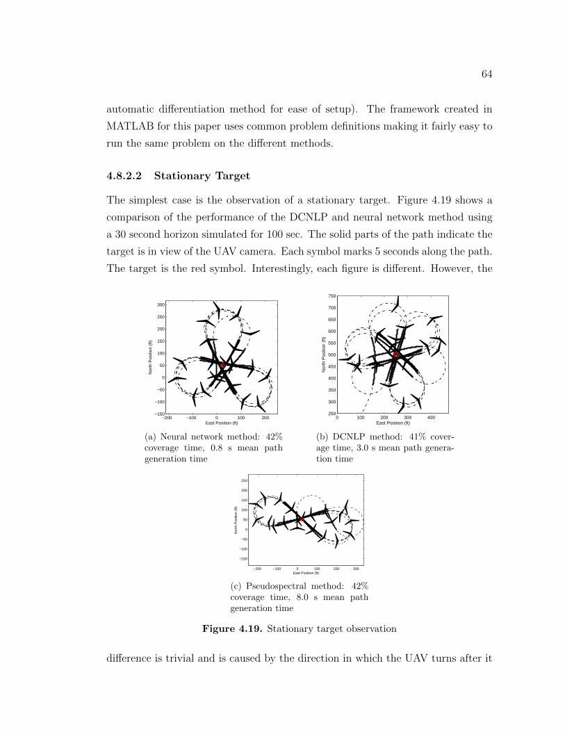
64
automatic differentiation method for ease of setup). The framework created in
MATLAB for this paper uses common problem definitions making it fairly easy to
run the same problem on the different methods.
4.8.2.2 Stationary Target
The simplest case is the observation of a stationary target. Figure 4.19 shows a
comparison of the performance of the DCNLP and neural network method using
a 30 second horizon simulated for 100 sec. The solid parts of the path indicate the
target is in view of the UAV camera. Each symbol marks 5 seconds along the path.
The target is the red symbol. Interestingly, each figure is different. However, the
−200 −100 0 100 200−150
−100
−50
0
50
100
150
200
250
300
Nor
th P
ositi
on (
ft)
East Position (ft)
(a) Neural network method: 42%coverage time, 0.8 s mean pathgeneration time
0 100 200 300 400250
300
350
400
450
500
550
600
650
700
750
Nor
th P
ositi
on (
ft)
East Position (ft)
(b) DCNLP method: 41% cover-age time, 3.0 s mean path genera-tion time
−200 −100 0 100 200 300
−150
−100
−50
0
50
100
150
200
250
Nor
th P
ositi
on (
ft)
East Position (ft)
(c) Pseudospectral method: 42%coverage time, 8.0 s mean pathgeneration time
Figure 4.19. Stationary target observation
difference is trivial and is caused by the direction in which the UAV turns after it
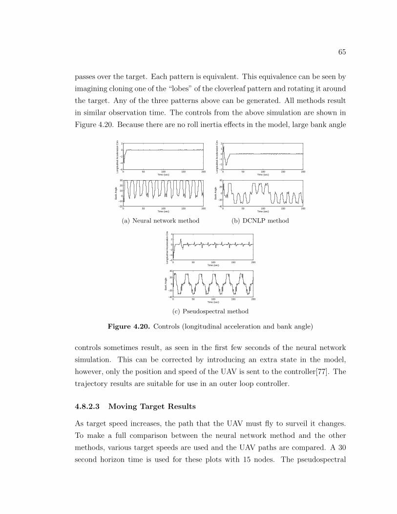
65
passes over the target. Each pattern is equivalent. This equivalence can be seen by
imagining cloning one of the “lobes” of the cloverleaf pattern and rotating it around
the target. Any of the three patterns above can be generated. All methods result
in similar observation time. The controls from the above simulation are shown in
Figure 4.20. Because there are no roll inertia effects in the model, large bank angle
0 50 100 150 200−6
−4
−2
0
2
Time (sec)
Long
itudi
nal A
ccel
erat
ion
Cm
d
0 50 100 150 200−20
−10
0
10
20
30
Time (sec)
Ban
k A
ngle
(a) Neural network method
0 50 100 150 200−3
−2
−1
0
1
2
Time (sec)
Long
itudi
nal A
ccel
erat
ion
Cm
d
0 50 100 150 200−40
−20
0
20
40
Time (sec)
Ban
k A
ngle
(b) DCNLP method
0 50 100 150 200−6
−4
−2
0
2
4
Time (sec)
Long
itudi
nal A
ccel
erat
ion
Cm
d
0 50 100 150 200−40
−20
0
20
40
Time (sec)
Ban
k A
ngle
(c) Pseudospectral method
Figure 4.20. Controls (longitudinal acceleration and bank angle)
controls sometimes result, as seen in the first few seconds of the neural network
simulation. This can be corrected by introducing an extra state in the model,
however, only the position and speed of the UAV is sent to the controller[77]. The
trajectory results are suitable for use in an outer loop controller.
4.8.2.3 Moving Target Results
As target speed increases, the path that the UAV must fly to surveil it changes.
To make a full comparison between the neural network method and the other
methods, various target speeds are used and the UAV paths are compared. A 30
second horizon time is used for these plots with 15 nodes. The pseudospectral
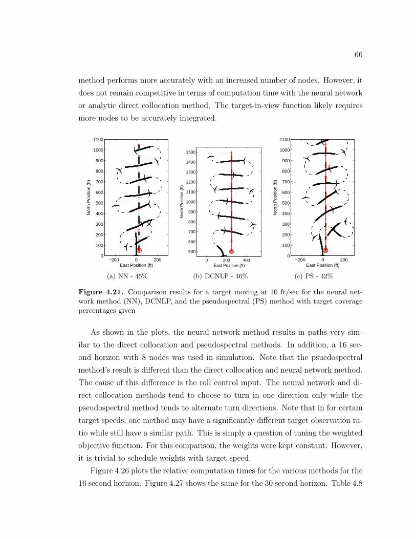
66
method performs more accurately with an increased number of nodes. However, it
does not remain competitive in terms of computation time with the neural network
or analytic direct collocation method. The target-in-view function likely requires
more nodes to be accurately integrated.
−200 0 2000
100
200
300
400
500
600
700
800
900
1000
1100
Nor
th P
ositi
on (
ft)
East Position (ft)
(a) NN - 45%
0 200 400
500
600
700
800
900
1000
1100
1200
1300
1400
1500
Nor
th P
ositi
on (
ft)
East Position (ft)
(b) DCNLP - 46%
−200 0 2000
100
200
300
400
500
600
700
800
900
1000
1100
Nor
th P
ositi
on (
ft)
East Position (ft)
(c) PS - 42%
Figure 4.21. Comparison results for a target moving at 10 ft/sec for the neural net-work method (NN), DCNLP, and the pseudospectral (PS) method with target coveragepercentages given
As shown in the plots, the neural network method results in paths very sim-
ilar to the direct collocation and pseudospectral methods. In addition, a 16 sec-
ond horizon with 8 nodes was used in simulation. Note that the psuedospectral
method’s result is different than the direct collocation and neural network method.
The cause of this difference is the roll control input. The neural network and di-
rect collocation methods tend to choose to turn in one direction only while the
pseudospectral method tends to alternate turn directions. Note that in for certain
target speeds, one method may have a significantly different target observation ra-
tio while still have a similar path. This is simply a question of tuning the weighted
objective function. For this comparison, the weights were kept constant. However,
it is trivial to schedule weights with target speed.
Figure 4.26 plots the relative computation times for the various methods for the
16 second horizon. Figure 4.27 shows the same for the 30 second horizon. Table 4.8

67
−200 02000
500
1000
1500
2000
2500
3000
3500
4000
Nor
th P
ositi
on (
ft)
East Position (ft)
(a) NN - 43%
0 200400500
1000
1500
2000
2500
3000
3500
4000
4500
Nor
th P
ositi
on (
ft)
East Position (ft)
(b) DCNLP - 54%
−200 02000
500
1000
1500
2000
2500
3000
3500
4000
Nor
th P
ositi
on (
ft)East Position (ft)
(c) PS - 52%
Figure 4.22. Comparison results for a target moving at 20 ft/sec for the neural net-work method (NN), DCNLP, and the pseudospectral (PS) method with target coveragepercentages given
summarizes the mean path generation time for the various cases. Relative to the
direct collocation method, the neural network approximation method requires be-
tween 2.5-5 times less computation time than the fastest method using analytic
derivatives. The ratio jumps to 60-80 times faster when using complex-step deriva-
tives. Automatic differentiation performed similarly to complex-step derivatives.
Table 4.9 lists the relative computation time for the different methods. Finally, all
methods generally produce the same amount of target coverage. The simulation
was run for 100 seconds. Coverage time is simply the time the target is in view
divided by the simulation time. Table 4.10 lists the coverage time for the various
methods for a 30 second horizon. The 16 second horizon results are not shown,
as the only main difference is the lessened prediction common to all methods. For
example, at Vtarg = 35ft/s and 16 second horizon, none of the methods are able

68
−20002000
500
1000
1500
2000
2500
3000
3500
4000
4500
5000
Nor
th P
ositi
on (
ft)
East Position (ft)
(a) NN - 63%
0200400500
1000
1500
2000
2500
3000
3500
4000
4500
5000
5500
Nor
th P
ositi
on (
ft)
East Position (ft)
(b) DCNLP - 67%
−20002000
500
1000
1500
2000
2500
3000
3500
4000
4500
5000
Nor
th P
ositi
on (
ft)East Position (ft)
(c) PS - 66%
Figure 4.23. Comparison results for a target moving at 25 ft/sec for the neural net-work method (NN), DCNLP, and the pseudospectral (PS) method with target coveragepercentages given
to achieve 100% observation time because they are unable predict far enough into
the future.
4.8.2.4 Dual UAV Comparison
Transforming the single UAV trajectory optimization into a multiple UAV formu-
lation is straightforward with the neural network method. No network retraining
is required for this extension to the problem because the problem is modular. The
varied parameter vector is augmented with the controls of the second UAV. In ad-
dition, the dynamics and objective networks are expanded with appropriate loops
so they are called repeatedly for multiple UAVs. Finally, the gradient calculation
for individual UAVs is generally combined in block diagonal form with constraints
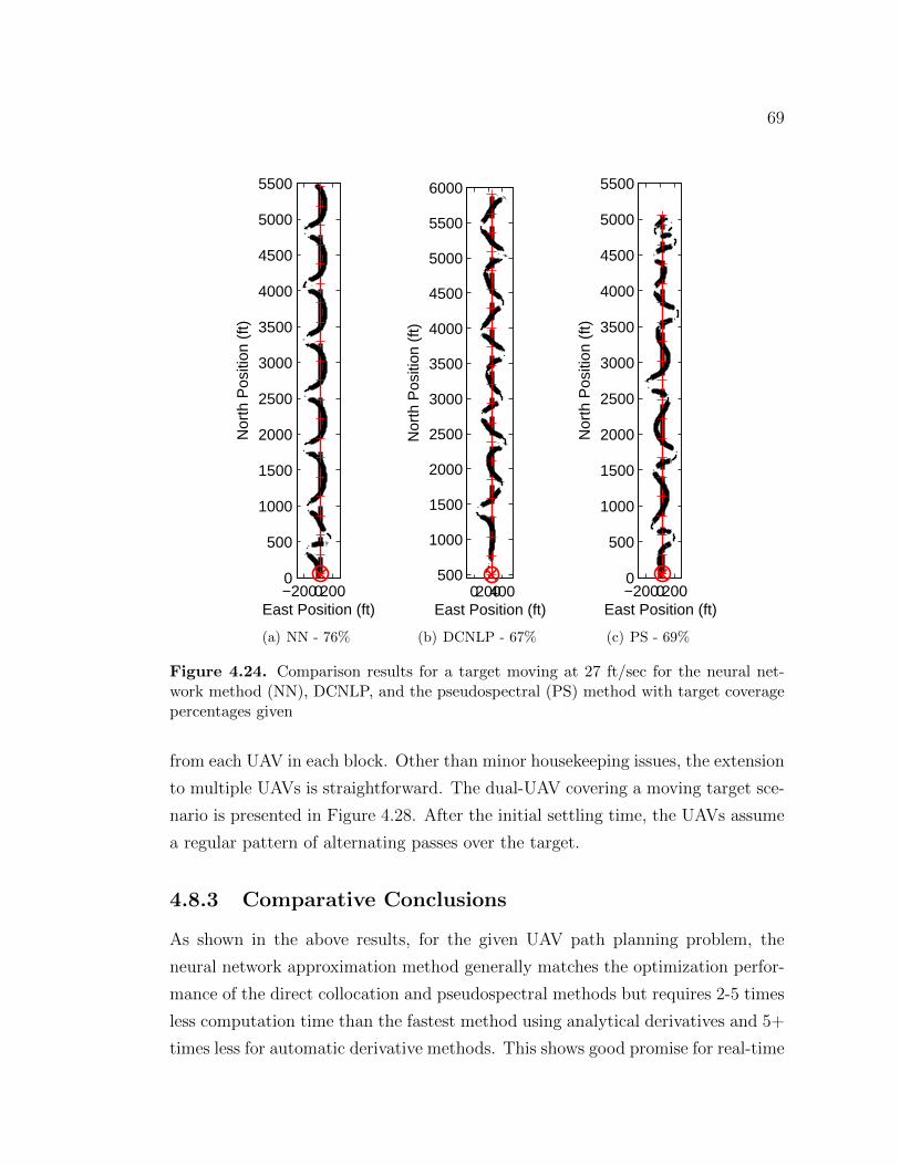
69
−20002000
500
1000
1500
2000
2500
3000
3500
4000
4500
5000
5500
Nor
th P
ositi
on (
ft)
East Position (ft)
(a) NN - 76%
0200400500
1000
1500
2000
2500
3000
3500
4000
4500
5000
5500
6000
Nor
th P
ositi
on (
ft)
East Position (ft)
(b) DCNLP - 67%
−20002000
500
1000
1500
2000
2500
3000
3500
4000
4500
5000
5500
Nor
th P
ositi
on (
ft)
East Position (ft)
(c) PS - 69%
Figure 4.24. Comparison results for a target moving at 27 ft/sec for the neural net-work method (NN), DCNLP, and the pseudospectral (PS) method with target coveragepercentages given
from each UAV in each block. Other than minor housekeeping issues, the extension
to multiple UAVs is straightforward. The dual-UAV covering a moving target sce-
nario is presented in Figure 4.28. After the initial settling time, the UAVs assume
a regular pattern of alternating passes over the target.
4.8.3 Comparative Conclusions
As shown in the above results, for the given UAV path planning problem, the
neural network approximation method generally matches the optimization perfor-
mance of the direct collocation and pseudospectral methods but requires 2-5 times
less computation time than the fastest method using analytical derivatives and 5+
times less for automatic derivative methods. This shows good promise for real-time
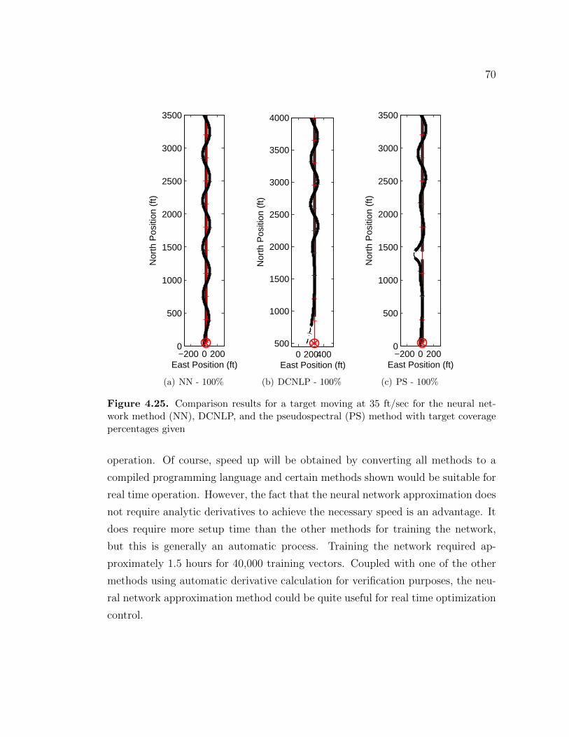
70
−200 0 2000
500
1000
1500
2000
2500
3000
3500
Nor
th P
ositi
on (
ft)
East Position (ft)
(a) NN - 100%
0 200400500
1000
1500
2000
2500
3000
3500
4000
Nor
th P
ositi
on (
ft)
East Position (ft)
(b) DCNLP - 100%
−200 0 2000
500
1000
1500
2000
2500
3000
3500
Nor
th P
ositi
on (
ft)East Position (ft)
(c) PS - 100%
Figure 4.25. Comparison results for a target moving at 35 ft/sec for the neural net-work method (NN), DCNLP, and the pseudospectral (PS) method with target coveragepercentages given
operation. Of course, speed up will be obtained by converting all methods to a
compiled programming language and certain methods shown would be suitable for
real time operation. However, the fact that the neural network approximation does
not require analytic derivatives to achieve the necessary speed is an advantage. It
does require more setup time than the other methods for training the network,
but this is generally an automatic process. Training the network required ap-
proximately 1.5 hours for 40,000 training vectors. Coupled with one of the other
methods using automatic derivative calculation for verification purposes, the neu-
ral network approximation method could be quite useful for real time optimization
control.

71
0 10 20 25 27 35
2468
10121416
75
Target Speed (ft/s)
Rel
ativ
eC
omputa
tion
Tim
e
Neural NetworkDCNLP Analytical
DCNLP Complex-stepPseudo. Auto. Diff
Pseudo. Complex-step
1
Figure 4.26. Relative computation time for various path planning methods using a 16second horizon

72
0 10 20 25 27 35
2468
1012
50
60
70
80
90
100
110
120
Target Speed (ft/s)
Rel
ativ
eC
omputa
tion
Tim
e
Neural NetworkDCNLP Analytical
DCNLP Complex-stepPseudo. Auto. Diff
Pseudo. Complex-step
1
Figure 4.27. Relative computation time for various path planning methods using a 30second horizon
−500 0 500 1000 1500 2000 2500 3000−400
−200
0
200
400
Nor
th P
ositi
on (
ft)
East Position (ft)
(a) Ground Path (9 nodes, 16 sec horizon, 93% coverage, 0.76 sec average calculationtime)
0 50 100 150 200Time (sec)
(b) Target coverage timeline
Figure 4.28. Ground track and coverage timeline for two UAVs and a target at 15 ft/s
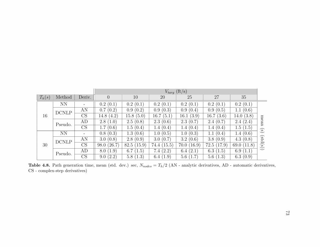
73
Vtarg (ft/s)Tℎ(s) Method Deriv. 0 10 20 25 27 35
16
NN - 0.2 (0.1) 0.2 (0.1) 0.2 (0.1) 0.2 (0.1) 0.2 (0.1) 0.2 (0.1)
mean
(s)(std
(s))
DCNLPAN 0.7 (0.2) 0.9 (0.2) 0.9 (0.3) 0.9 (0.4) 0.9 (0.5) 1.1 (0.6)CS 14.8 (4.2) 15.8 (5.0) 16.7 (5.1) 16.1 (3.9) 16.7 (3.6) 14.0 (3.8)
Pseudo.AD 2.8 (1.0) 2.5 (0.8) 2.3 (0.6) 2.3 (0.7) 2.4 (0.7) 2.4 (2.4)CS 1.7 (0.6) 1.5 (0.4) 1.4 (0.4) 1.4 (0.4) 1.4 (0.4) 1.5 (1.5)
30
NN - 0.8 (0.3) 1.3 (0.6) 1.0 (0.5) 1.0 (0.3) 1.1 (0.4) 1.4 (0.6)
DCNLPAN 3.0 (0.8) 2.8 (0.9) 3.0 (0.7) 3.2 (0.6) 3.8 (0.9) 4.3 (0.8)CS 98.0 (26.7) 82.5 (15.9) 74.4 (15.5) 70.0 (16.9) 72.5 (17.9) 69.0 (11.8)
Pseudo.AD 8.0 (1.9) 6.7 (1.5) 7.4 (2.2) 6.4 (2.1) 6.3 (1.5) 6.9 (1.1)CS 9.0 (2.2) 5.8 (1.3) 6.4 (1.9) 5.6 (1.7) 5.6 (1.3) 6.3 (0.9)
Table 4.8. Path generation time, mean (std. dev.) sec, Nnodes = Tℎ/2 (AN - analytic derivatives, AD - automatic derivatives,CS - complex-step derivatives)

74
Vtarg (ft/s)Tℎ(s) Method Deriv. 0 10 20 25 27 35
16
NN - 1.0 1.0 1.0 1.0 1.0 1.0 Relative
Com
putation
Tim
e
DCNLPAN 3.5 4.5 4.5 4.5 4.5 5.5CS 74.0 79.0 83.5 80.5 83.5 70.0
Pseudo.AD 14.0 12.5 11.5 11.5 12.0 12.0CS 8.5 7.5 7.0 7.0 7.0 7.5
30
NN - 1.0 1.0 1.0 1.0 1.0 1.0
DCNLPAN 3.8 2.2 3.0 3.2 3.5 3.1CS 122.5 63.5 74.4 70.0 65.9 49.3
Pseudo.AD 10.0 5.2 7.4 6.4 5.7 4.9CS 11.3 4.5 6.4 5.6 5.1 4.5
Table 4.9. Relative path generation time compared to neural network method,Nnodes = Tℎ/2 (AN - analytic derivatives, AD - automatic derivatives, CS - complex-stepderivatives)
Vtarg (ft/s)Tℎ(s) Method 0 10 20 25 27 35
16NN 35% 42% 50% 61% 63% 87%
Coverage
%
DCNLP 38% 40% 39% 53% 43% 74%Pseudo. 41% 43% 48% 48% 46% 76%
30NN 40% 33% 46% 64% 73% 100%
DCNLP 39% 37% 50% 69% 76% 100%Pseudo. 42% 42% 50% 65% 67% 100%
Table 4.10. Target coverage (percentage of total simulation time)

Chapter 5Real time implementation and Flight
Test
Simulation of a trajectory optimization method is quite different than actual im-
plementation. For example, simulation bypasses any requirements for real time
operation and does not require consideration of issues related to communicating
with hardware or other software. This chapter looks at the implementation of
the direct collocation method for use in real-time aboard the Applied Research
Laboratory/Penn State (ARL/PSU) testbed UAV. Results from flight testing are
presented. These results were originally published in Reference [77] which was
combined from two earlier conference papers ([37, 80]).
5.1 UAV Testbed Description
The ARL/PSU testbed UAV is a modified Sig Kadet Senior. The Kadet is a
basic balsa-construction .60-size trainer aircraft that comes in almost-ready-to-fly
(ARF) kit form. The ARF kit allows for easy modification and replacement parts
if needed. The modified aircraft has a payload of about five pounds, gross weight
of 14 pounds, and an 80 inch wingspan. The payload includes a CloudCapTech
Piccolo Plus autopilot, Ampro ReadyBoard 800 single board computer equipped
with a 1.4 GHz processor and 1 GB memory, a USB webcam or a digital camera,
and 4000 mAh lithium polymer battery. Figure 5.1 shows external and internal
views of the aircraft. Visible in Figure 5.1(b) are the Ampro ReadyBoard 800

76
towards the left, the autopilot in the middle, and the white fuel tank in the back-
ground on the right. The Kadet is heavily modified from its kit form. Heavy duty
landing gear/mounting hardware, .90-size 4-stroke engine, and rearrangement of
internal servo mounts are necessary for maximum payload volume and weight.
Figure 5.2(a) shows the modified main landing gear along with the payload bays.
Starting from the left: (1) servo battery and nosegear servo housing, (2) camera,
webcam, or mission specific payload bay, (3) fuel tank. The space behind the main
landing gear mount is empty. Figure 5.2(b) shows the empennage servos’ loca-
tions. Figure 5.1(c) shows the cowling, the modified nosegear, and webcam/digital
camera mount. Behind the cowling, a larger engine mount is installed and the
throttle servo is relocated to the outside of the firewall (normally inside the air-
craft). Additional modifications include the mounting of GPS, 900 MHz, and
802.11b antenna ground planes. As shown in Figure 5.1(a), these can be seen on
the on right side of horizontal stabilizer, large antenna just behind the wing, front
tip of the vertical tail, for the GPS, 900 MHz, and 802.11b antennae respectively.
The pitot-static system, provided by CloudCap Technologies, consists of a carbon
fiber pitot-static probe with corresponding mounting hardware installed on the
right wing.
During the assembly of the UAVs, the onboard computer was found to interfere
with GPS reception. GPS satellites broadcast on two frequencies: L1 at 1.57542
GHz and L2 at 1.2276 GHz. Because the processor operates at 1.4 GHz, inter-
ference is likely (and did occur) if the GPS antenna is too close to the computer.
The problem was solved by putting the GPS antenna on the horizontal tail of the
Kadet. This setup has been operated without additional interference problems and
generally receives signals from between 6 & 10 GPS satellites. Note that 4 satel-
lites are required for a 3-dimensional position fix, and the GPS unit in the Piccolo
Plus autopilot is capable of tracking 12 satellites simultaneously (a Motorola M12
Oncore).
Onboard power is supplied by a 12V, 4000 mAh lithium-polymer (LiPo) battery,
providing approximately 1.5 to 2 hours of system operating time, depending on
processor load. The Ampro single board computer is powered by a V-Infinity 12V-
to-5V DC power converter, which is connected to the LiPo battery. The power
converter can be remotely powered on or off from the Piccolo Command Center

77
(a) Exterior View
(b) Interior view with autopilot and computer visible
(c) Bottom view showing camera mount and 12V-to-5V power supply
Figure 5.1. The Applied Research Lab/Penn State UAV Testbed
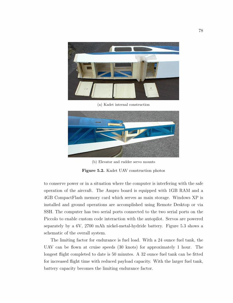
78
(a) Kadet internal construction
(b) Elevator and rudder servo mounts
Figure 5.2. Kadet UAV construction photos
to conserve power or in a situation where the computer is interfering with the safe
operation of the aircraft. The Ampro board is equipped with 1GB RAM and a
4GB CompactFlash memory card which serves as main storage. Windows XP is
installed and ground operations are accomplished using Remote Desktop or via
SSH. The computer has two serial ports connected to the two serial ports on the
Piccolo to enable custom code interaction with the autopilot. Servos are powered
separately by a 6V, 2700 mAh nickel-metal-hydride battery. Figure 5.3 shows a
schematic of the overall system.
The limiting factor for endurance is fuel load. With a 24 ounce fuel tank, the
UAV can be flown at cruise speeds (30 knots) for approximately 1 hour. The
longest flight completed to date is 50 minutes. A 32 ounce fuel tank can be fitted
for increased flight time with reduced payload capacity. With the larger fuel tank,
battery capacity becomes the limiting endurance factor.

79
2.4 GHz802.11b
2.4 GHz802.11b
900 MHzLink
V-Infinity12 V to 5 V
DC power supply
900 MHzLink
GPS
PiccoloAutopilot
GroundStation
AmproReadyboard
CloudCapCommSDK over RS-232
Servo Output
Camera orwebcam
USB6V, 2700 mAhNiMh Servo
Battery
12V, 4000 mAhLiPo Battery
Laptop:Operator Interface &
Remote Desktop
RS-232
Onboard System
Figure 5.3. Block diagram for the airborne and ground systems
The onboard camera is hard mounted to the airframe and points downward. A
Logitech Ultra Vision USB webcam with a 63∘ horizontal and 50∘ vertical field of
view is used. Video output has a resolution of 640 by 480 pixels, and is captured
using OpenCV[81], an open source computer vision library created by Intel in
C++. The UAV also is able to accept a 4 megapixel Canon digital camera.
The ARL/PSU UAV team has three Piccolo equipped UAVs, two with on-board
single board computers. The Sig Kadet platform has proved itself to be a reliable
platform for research. Over the years of 2006-2008, the team has logged nearly
50 flights with the Kadet UAVs, including simultaneous operation of two UAVs to
facilitate path planner testing and future collaborative research efforts[36]. Though
not flown yet, the ARL/PSU group is building two larger UAVs based on the Super
Flyin’ King kit from Bruce Tharpe. These aircraft will support expansion of the
Intelligent Controller work done by Miller [35].
All flight operations take place at the Centre Airpark airfield, a private grass
strip located near Old Fort, Pennsylvania. The runway is 3100 ft long and 210
feet wide. Large red barrels line the run way boundary. These barrels are used as
observation targets in some tests because they are painted red and can easily been
seen by the camera onboard the UAV. Figure 5.4 shows an aerial photo of Centre
Airpark, the target exercise balls, and a runway boundary barrel.

80
(a) USGS Aerial photo of Centre Airpark, runway outlined in green & 5 barrellocations shown with dots
(b) Dual-ball target
(c) Barrel target
Figure 5.4. Airfield Photos and test target photos

81
5.2 Implementation Issues & Initial Flight Tests
Initially, a separate path navigator program was written. It read the path output
from the optimization and sent turn rate commands to the autopilot. The reason
for this was to have greater control over how the path is followed. Only limited
control is available through the gains on the autopilot. However, the onboard
computer must run the path planner, the path navigator, and any image capture
software. In light of the requirement to run the path planner in real time, it would
be best to offload as many tasks from the onboard computer as possible. Ad-
ditionally, there would be increased programming complexity as communications
between the path navigator and planner would be required. The autopilot is pro-
vided with a software development kit which makes communications with external
devices easy to implement. Therefore, only the North and East coordinates of the
path nodes output from the path planner are sent to the autopilot. The autopilot
is then commanded to fly this path.
The connection between the path planning algorithm and the Piccolo autopilot
is then fairly simple. Once a path is computed, the x, y coordinates of each node are
converted to latitude and longitude. The string of points is converted to the proper
format and sent to the Piccolo (using the Cloud Cap Software Development Kit).
Since there is a time lag between receiving the current UAV position, computing
the path, and sending the waypoint list, the path planner chooses the correct
waypoint on the list to command the autopilot to fly to. The chosen waypoint is
one not yet reached on the newly updated path. The autopilot will then follow
this path until the next update. Speed commands are sent directly by periodically
checking where the UAV is on the computed path and sending the appropriate
speed command.
5.2.1 Real-Time Implementation
A C++ version of the path planning algorithm capable of running in real time has
been developed and tested. As discussed in Section 4.6, the SNOPT[13] package
is used as the nonlinear solver based on personal experience and recommendations
of others who have used it. Since SNOPT has a C++ and MATLAB interface, it
can be integrated with both the C++ path planner implementation and with the
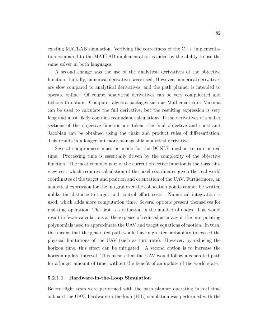
82
existing MATLAB simulation. Verifying the correctness of the C++ implementa-
tion compared to the MATLAB implementation is aided by the ability to use the
same solver in both languages.
A second change was the use of the analytical derivatives of the objective
function. Initially, numerical derivatives were used. However, numerical derivatives
are slow compared to analytical derivatives, and the path planner is intended to
operate online. Of course, analytical derivatives can be very complicated and
tedious to obtain. Computer algebra packages such as Mathematica or Maxima
can be used to calculate the full derivative, but the resulting expression is very
long and most likely contains redundant calculations. If the derivatives of smaller
sections of the objective function are taken, the final objective and constraint
Jacobian can be obtained using the chain and product rules of differentiation.
This results in a longer but more manageable analytical derivative.
Several compromises must be made for the DCNLP method to run in real
time. Processing time is essentially driven by the complexity of the objective
function. The most complex part of the current objective function is the target-in-
view cost which requires calculation of the pixel coordinates given the real world
coordinates of the target and position and orientation of the UAV. Furthermore, an
analytical expression for the integral over the collocation points cannot be written
unlike the distance-to-target and control effort costs. Numerical integration is
used, which adds more computation time. Several options present themselves for
real-time operation. The first is a reduction in the number of nodes. This would
result in fewer calculations at the expense of reduced accuracy in the interpolating
polynomials used to approximate the UAV and target equations of motion. In turn,
this means that the generated path would have a greater probability to exceed the
physical limitations of the UAV (such as turn rate). However, by reducing the
horizon time, this effect can be mitigated. A second option is to increase the
horizon update interval. This means that the UAV would follow a generated path
for a longer amount of time, without the benefit of an update of the world state.
5.2.1.1 Hardware-in-the-Loop Simulation
Before flight tests were performed with the path planner operating in real time
onboard the UAV, hardware-in-the-loop (HIL) simulation was performed with the
83
Configuration Nodes Horizon Length Update Interval
1. 11 30.0 sec. 6.0 sec.2. 7 20.0 sec. 4.0 sec.
Table 5.1. Path planner configurations used in flight testing
same computer that is flown on the UAV. Several combinations of horizon time,
number of nodes, and horizon update interval were tested to find settings that
would be best to flight test. A stationary target was used in the simulation. These
HIL simulations test the ability of the path planner to generate a viable path and
to do so within the horizon update interval. The standard setup used in simulation
was 11 nodes, a 30 second horizon time, and a horizon update every 1.5 seconds.
Using 11 nodes, the algorithm takes around 3 seconds on average and up to 6
seconds to generate a new path. This produced a very smooth cloverleaf pattern
around a stationary target, however it was too slow to use in real-time operation
because of the very short path update interval. Increasing the update interval to
6 seconds allowed the path planner to generate a new path before another update
was required. While this was satisfactory, the path generation was still fairly slow
at 3 seconds per path. To obtain a shorter path generation time, the path planner
was tested using 7 nodes and a 20 second horizon time. On average, the path
planner requires around 1 second to generate a new path in this configuration.
Using an update interval of 4 seconds with these settings generates a viable path
while maintaining a buffer between the time required to generate a path and the
path update interval. The two configurations tested in flight tests are given in
Table 5.1. The results section discusses the advantages and disadvantages of these
configurations.
5.3 Flight Test Results
The limits shown in Table 5.2 were used in the following flight test results. They
are based on the estimated performance limitations of the Sig Kadet Senior. As a
safety margin, the bank angle limit is lower than that which the UAV is capable.
The path planner was flight tested while operating in real time onboard the
UAV. The test scenarios performed include a stationary target in calm and steady

84
Constraint Value
Stall Speed Vmin = 22ktsMaximum Speed Vmax = 50kts
Maximum Longitudinal ulmax = 10ft/s2
Acceleration ulmin = −10ft/s2
Maximum Bank Angle � = ±30∘
Table 5.2. UAV performance constraints
wind conditions, a walking person, a moving vehicle, and a second UAV flying at
a lower altitude. The results of these tests are discussed below. Figures that show
the ground track of the UAV use a greyscale aerial photo of the flying field as the
background. The end of the ground track is indicated by a triangle. Also visible
are 5 dots which mark the locations of barrels used for targets. If they are relevant
to the results, they are circled and labeled. For cases with two UAVs where one
UAV acts as a target, the tracker UAV is shown as a solid line and the target UAV
is shown as a dashed line.
For these results, the path planner was given the target’s location through a
ground station uplink. In Section 5.4, results using integrated path planning and
target geolocation are presented. In order to relay the target location from the
ground to the UAV above, a second Piccolo autopilot was used as the target, be it
handheld, in a truck, or on a second UAV. The ground station communicates with
both Piccolos simultaneously. It also has the ability to run a sever on the local
wireless network which serves the data it receives from the autopilots. The tracking
UAV connects to the ground station server over its onboard 802.11b connection,
and requests all data specific to the Piccolo being used as a target. This data
includes GPS location and ground speed.
5.3.1 Stationary Target
For this test, an airfield barrel was chosen as the target to observe. Its latitude and
longitude was input to the path planner prior to starting the test. Figure 5.5(a)
shows the ground track of the UAV while under the direction of the path planner.
The familiar clover leaf pattern seen in simulation is readily apparent. Figure 5.5(b)
is a histogram showing the time required to calculate each new path update. A

85
majority of the path updates require under one second and no path update took
longer than the update interval (4 seconds for this flight), showing that the planner
is operating in real time. For both configurations, the camera has a view of the
(a) Ground track
0 1 2 3 40
5
10
15
20
25
30
35
Time required to compute path (seconds)
Cyc
le C
ount
(b) Path generation time
Figure 5.5. Stationary target observation in calm winds
target 41% of the time. This percentage is measured by watching the recorded
onboard video after the flight and measuring the length of each time the target is
86
in view and dividing by the length of time from the first view of the target to the
end of the test.
5.3.2 Stationary Target in steady winds
Figure 5.6(a) shows the results of observing a stationary target in a 5 knot wind
coming from the west (the left side of the figure). Note that the Kalman filter
on Piccolo autopilot is able to estimate wind speed using airspeed and GPS mea-
surements. The wind estimate is then used in the optimization. Previously, flight
tests were conducted without accounting for steady winds resuling in very poor
target observation time. Using wind estimates, the figure-8 pattern seen in sim-
ulation emerges here in the flight test. Also note that all of the turns are made
into the wind; this minimizes the ground track turn radius. Comparing the path
update time histogram (Figure 5.6(b)) with the calm wind case shows that com-
pensating for wind requires slightly more processing time, which is to be expected.
Configuration 2 was used in both of the results shown for the stationary target
tests (7 nodes, 20 second horizon time, 4 second update interval). Configuration 1
produced similar results and was able to operate in real time. The only significant
difference was the amount of processing time required. For configuration 1, the
onboard camera has a view of the target 41% of the time, while for configuration
2 achieves 40% time coverage.
5.3.3 Tracking a moving ground target
For the second set of flight tests, a spare Piccolo autopilot was used as a mobile
target. The laptop connected to the ground station runs a server on the 802.11
wireless network that mirrors the data received from the autopilots. The computer
onboard the tracker UAV connects to this server over the 802.11 network and is
able to receive all data from the target autopilot.
Both a person walking with the target Piccolo and a truck driving down the
adjacent road were used to test the mobile target tracking ability of the path
planner. We found that a person walking was not fast enough to produce much
variation in the path (other than the motion of the path center) of the UAV
compared to a stationary target. Figure 5.7(a) shows a typical result. The person,
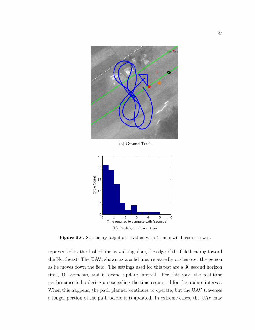
87
(a) Ground Track
0 1 2 3 4 5 60
5
10
15
20
25
Time required to compute path (seconds)
Cyc
le C
ount
(b) Path generation time
Figure 5.6. Stationary target observation with 5 knots wind from the west
represented by the dashed line, is walking along the edge of the field heading toward
the Northeast. The UAV, shown as a solid line, repeatedly circles over the person
as he moves down the field. The settings used for this test are a 30 second horizon
time, 10 segments, and 6 second update interval. For this case, the real-time
performance is bordering on exceeding the time requested for the update interval.
When this happens, the path planner continues to operate, but the UAV traverses
a longer portion of the path before it is updated. In extreme cases, the UAV may
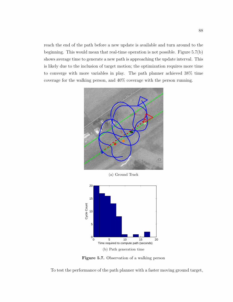
88
reach the end of the path before a new update is available and turn around to the
beginning. This would mean that real-time operation is not possible. Figure 5.7(b)
shows average time to generate a new path is approaching the update interval. This
is likely due to the inclusion of target motion; the optimization requires more time
to converge with more variables in play. The path planner achieved 38% time
coverage for the walking person, and 40% coverage with the person running.
(a) Ground Track
0 5 10 15 200
5
10
15
20
Time required to compute path (seconds)
Cyc
le C
ount
(b) Path generation time
Figure 5.7. Observation of a walking person
To test the performance of the path planner with a faster moving ground target,
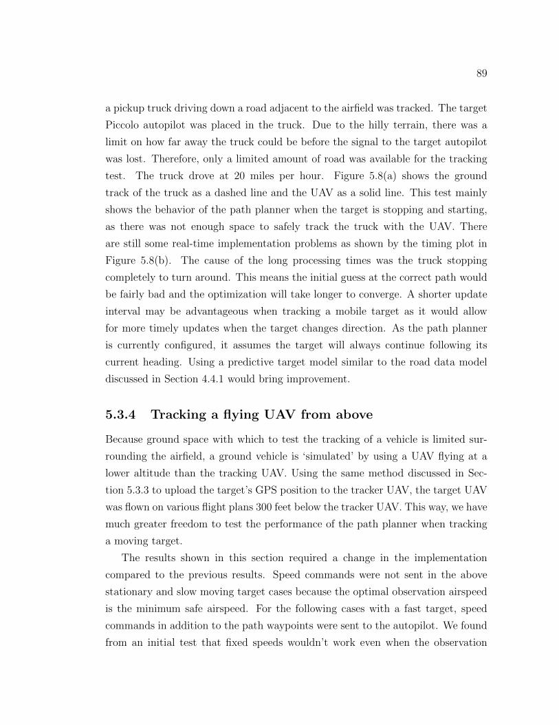
89
a pickup truck driving down a road adjacent to the airfield was tracked. The target
Piccolo autopilot was placed in the truck. Due to the hilly terrain, there was a
limit on how far away the truck could be before the signal to the target autopilot
was lost. Therefore, only a limited amount of road was available for the tracking
test. The truck drove at 20 miles per hour. Figure 5.8(a) shows the ground
track of the truck as a dashed line and the UAV as a solid line. This test mainly
shows the behavior of the path planner when the target is stopping and starting,
as there was not enough space to safely track the truck with the UAV. There
are still some real-time implementation problems as shown by the timing plot in
Figure 5.8(b). The cause of the long processing times was the truck stopping
completely to turn around. This means the initial guess at the correct path would
be fairly bad and the optimization will take longer to converge. A shorter update
interval may be advantageous when tracking a mobile target as it would allow
for more timely updates when the target changes direction. As the path planner
is currently configured, it assumes the target will always continue following its
current heading. Using a predictive target model similar to the road data model
discussed in Section 4.4.1 would bring improvement.
5.3.4 Tracking a flying UAV from above
Because ground space with which to test the tracking of a vehicle is limited sur-
rounding the airfield, a ground vehicle is ‘simulated’ by using a UAV flying at a
lower altitude than the tracking UAV. Using the same method discussed in Sec-
tion 5.3.3 to upload the target’s GPS position to the tracker UAV, the target UAV
was flown on various flight plans 300 feet below the tracker UAV. This way, we have
much greater freedom to test the performance of the path planner when tracking
a moving target.
The results shown in this section required a change in the implementation
compared to the previous results. Speed commands were not sent in the above
stationary and slow moving target cases because the optimal observation airspeed
is the minimum safe airspeed. For the following cases with a fast target, speed
commands in addition to the path waypoints were sent to the autopilot. We found
from an initial test that fixed speeds wouldn’t work even when the observation

90
(a) Ground Track
0 5 10 15 200
0.5
1
1.5
2
2.5
3
Time required to compute path (seconds)
Cyc
le C
ount
(b) Path generation time
Figure 5.8. Observation of a moving truck (20 mph); Time required to generate a newpath
and target UAVs’ speeds were the same. Note that speed commands cannot be
updated when the path is being calculated. Since the target’s speed does not vary
quickly, this limitation did not cause a problem. The limitation could be overcome
by using an intermediary program to send commands to the autopilot.
The initial test tracked a UAV around a simple rectangular pattern. For this
test, the tracker UAV was allowed to match the speed of the target UAV. Figure 5.9
shows the start of the maneuver. The tracker UAV is shown by the solid line and
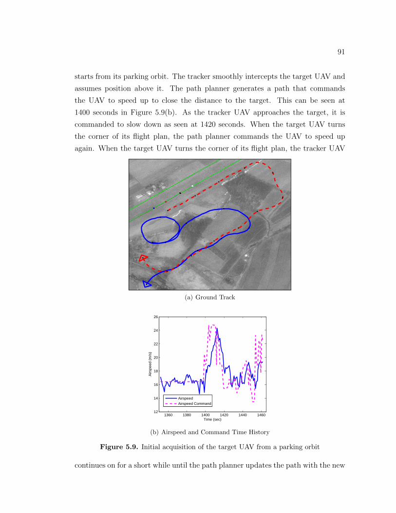
91
starts from its parking orbit. The tracker smoothly intercepts the target UAV and
assumes position above it. The path planner generates a path that commands
the UAV to speed up to close the distance to the target. This can be seen at
1400 seconds in Figure 5.9(b). As the tracker UAV approaches the target, it is
commanded to slow down as seen at 1420 seconds. When the target UAV turns
the corner of its flight plan, the path planner commands the UAV to speed up
again. When the target UAV turns the corner of its flight plan, the tracker UAV
(a) Ground Track
1360 1380 1400 1420 1440 146012
14
16
18
20
22
24
26
Airs
peed
(m
/s)
Time (sec)
AirspeedAirspeed Command
(b) Airspeed and Command Time History
Figure 5.9. Initial acquisition of the target UAV from a parking orbit
continues on for a short while until the path planner updates the path with the new
92
heading of the target. Figure 5.10 shows the UAVs on their second time around the
pattern. The tracker UAV overshoots the target when the target turns a corner,
but accelerates to make up ground and decelerates to reacquire the target. This
behavior can be clearly seen in Figure 5.10(b). Onboard video was not available
(a) Ground Track
1550 1570 1590 1610 1630 1650 1670 169012
14
16
18
20
22
24
26
Airs
peed
(m
/s)
Time (sec)
AirspeedAirspeed Command
(b) Airspeed and Command Time History
Figure 5.10. Tracking of the target UAV around a rectangular path
for this test because the UAV lost engine power and had a hard landing, causing
the video to be lost. However, based on the ground track, the target is estimated
to be covered 35% to 45% of the time.
A following flight retested this scenario with a slightly different rectangular
pattern. When the UAV was allowed to match the target’s speed, the coverage
time was measured to be 33%. When the UAV is limited to 10 knots faster than
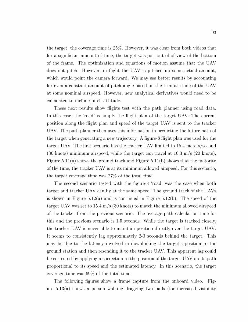
93
the target, the coverage time is 25%. However, it was clear from both videos that
for a significant amount of time, the target was just out of of view of the bottom
of the frame. The optimization and equations of motion assume that the UAV
does not pitch. However, in flight the UAV is pitched up some actual amount,
which would point the camera forward. We may see better results by accounting
for even a constant amount of pitch angle based on the trim attitude of the UAV
at some nominal airspeed. However, new analytical derivatives would need to be
calculated to include pitch attitude.
These next results show flights test with the path planner using road data.
In this case, the ‘road’ is simply the flight plan of the target UAV. The current
position along the flight plan and speed of the target UAV is sent to the tracker
UAV. The path planner then uses this information in predicting the future path of
the target when generating a new trajectory. A figure-8 flight plan was used for the
target UAV. The first scenario has the tracker UAV limited to 15.4 meters/second
(30 knots) minimum airspeed, while the target can travel at 10.3 m/s (20 knots).
Figure 5.11(a) shows the ground track and Figure 5.11(b) shows that the majority
of the time, the tracker UAV is at its minimum allowed airspeed. For this scenario,
the target coverage time was 27% of the total time.
The second scenario tested with the figure-8 ‘road’ was the case when both
target and tracker UAV can fly at the same speed. The ground track of the UAVs
is shown in Figure 5.12(a) and is continued in Figure 5.12(b). The speed of the
target UAV was set to 15.4 m/s (30 knots) to match the minimum allowed airspeed
of the tracker from the previous scenario. The average path calculation time for
this and the previous scenario is 1.5 seconds. While the target is tracked closely,
the tracker UAV is never able to maintain position directly over the target UAV.
It seems to consistently lag approximately 2-3 seconds behind the target. This
may be due to the latency involved in downlinking the target’s position to the
ground station and then resending it to the tracker UAV. This apparent lag could
be corrected by applying a correction to the position of the target UAV on its path
proportional to its speed and the estimated latency. In this scenario, the target
coverage time was 69% of the total time.
The following figures show a frame capture from the onboard video. Fig-
ure 5.13(a) shows a person walking dragging two balls (for increased visibility

94
(a) Ground Track
2560 2580 2600 2620 2640 2660 2680 2700 272014
16
18
20
22
24
Airs
peed
(m
/s)
Time (sec)
Airspeed
Airspeed Command
(b) Airspeed and Command Time History
Figure 5.11. Tracking of the target UAV around a figure-8 pattern with a 5 m/s (10knot) speed difference
in the video). Figure 5.13(b) shows a target UAV flying 300 ft below. The person
and UAV are circled in white.
5.4 Integrated Target Tracking and Path Plan-
ning
The previous flight test results are run with the target location being sent to the
UAV in flight. An integrated implementation is now discussed that is able to
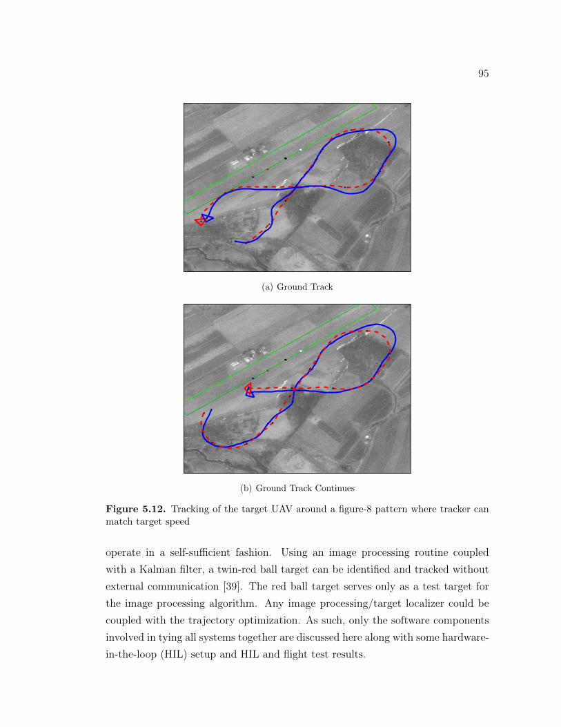
95
(a) Ground Track
(b) Ground Track Continues
Figure 5.12. Tracking of the target UAV around a figure-8 pattern where tracker canmatch target speed
operate in a self-sufficient fashion. Using an image processing routine coupled
with a Kalman filter, a twin-red ball target can be identified and tracked without
external communication [39]. The red ball target serves only as a test target for
the image processing algorithm. Any image processing/target localizer could be
coupled with the trajectory optimization. As such, only the software components
involved in tying all systems together are discussed here along with some hardware-
in-the-loop (HIL) setup and HIL and flight test results.
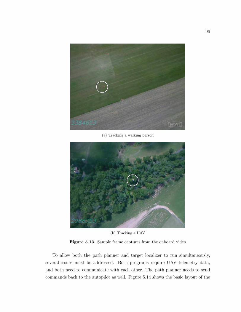
96
(a) Tracking a walking person
(b) Tracking a UAV
Figure 5.13. Sample frame captures from the onboard video
To allow both the path planner and target localizer to run simultaneously,
several issues must be addressed. Both programs require UAV telemetry data,
and both need to communicate with each other. The path planner needs to send
commands back to the autopilot as well. Figure 5.14 shows the basic layout of the

97
required connections. Timely communication between the processes is paramount,
HostController
TargetLocation
UAV State
PathPlanner
Update Flag
Waypoints &Speed Cmds
FlightgearComputer
VisionProcessing
USB
Webcam
Piccolo
State Data
Waypoints &Speed Cmds
SimulationComputerSim
ulation
State
Figure 5.14. Schematic of the hardware-in-the-loop simulation
so a shared memory scheme was chosen. The host controller receives telemetry from
the autopilot over a serial connection and places the data structure in a shared
memory location so the path planner and target geolocation processes can access
it. By continually updating the telemetry, each process always has the most recent
available data without the need for polling or requesting it. The target location
shared memory is continually updated with estimated target location from the
Kalman filter. The path planner reads the target location information and creates
a path. When path generation is finished, the path planner loads the path into
shared memory, and then sets the shared update flag. The host controller checks
this flag each cycle; if set, the shared memory containing the path is read and
sent to the autopilot. To avoid deadlock issues, no process depends on another to
continue running. Timing data is recorded for all processes to measure how the
integrated setup performs.
5.4.1 Hardware-in-the-loop simulation description
In the hardware-in-the-loop (HIL) setup, the autopilot is connected to a computer
that simulates flight dynamics. The Ampro ReadyBoard is connected to the au-

98
topilot and runs the image processing and path planning software. The camera
is connected to the USB port of the ReadyBoard and is pointed at a LCD which
displays aerial images generated by Flightgear[82], thus simulating what it would
actually see in flight. Figure 5.15(a) shows the setup. Figure 5.15(b) shows an
example of alignment calculation using the camera calibration toolbox.
(a) Webcam with on-screen calibration pat-tern
O
X
Y
Z
Image points (+) and reprojected grid points (o)
100 200 300 400 500 600
50
100
150
200
250
300
350
400
450
(b) Camera calibration result
Figure 5.15. Webcam HIL rig and calibration result
Several problems present themselves with this setup. The most basic is the
choice of screen. A CRT screen cannot be used as the webcam will pick up flickering
as the screen is redrawn. While tuning a camera to prevent flickering is possible,
most cheap webcams do not have this option. Therefore, an LCD is used to avoid
flickering. The second problem to solve is correct positioning of the camera; it
should be aligned with the normal vector of the LCD screen’s surface. To compute
the orientation of the camera with respect to the screen’s surface, the camera
calibration toolbox is used with the calibration pattern (shown in Figure 5.15(a)).
The required roll, pitch, and yaw corrections for the camera of the camera is easily
computed. An alignment to within 0.3 degrees in all axes was attained. The field
of view in Flightgear is then set to match the field of view of the camera.
The final component of the HIL system is the actual visualization of the ter-
rain. Flightgear comes with default world scenery that is fairly sparse. It does
have limited support for photorealistic scenery over small areas. Using 1 ft/pixel
resolution aerial photos of the flying field from Pennsylvania Spatial Data Access
99
(PASDA) [83], a 4096 ft2 area centered at the runway was imported into Flight-
gear using the photomodel command (available when Flightgear is compiled from
the source). Note that the area should be a power of two (in this case, 4096
pixels square) for the texture to be properly displayed in Flightgear. Shown in
Figure 5.16 is a comparison between actual picture recorded in flight and visuals
produced by Flightgear using the photorealistic scenery. The webcam reduces the
contrast and detail of the Flightgear visuals, however it is still usable by the target
recognition algorithm. The darkening in the top half of Figure 5.16(c) is due to
the viewing angle limitations of the LCD screen. One problem with using photore-
alistic scenery in Flightgear is that it is difficult to apply the aerial photo over an
elevation model. Therefore, the model used here is simply a flat plane. The focus
of the HIL simulation is not to test absolute localization accuracy, but to provide
a platform for debugging the system in a “realistic-enough” environment.
(a) Actual image captured in flight (b) Flightgear screen shot
(c) Flightgear as seen through the webcam
Figure 5.16. Comparison of actual and simulated aerial views

100
5.4.2 Path Planning
The integrated path planner and target geolocation code results are presented here
for the HIL simulation test. Figure 5.17(a) shows the ground path of the UAV; the
path planner generates a clover leaf pattern similar to that seen in simulation and
flight tests where the target location was known. Figure 5.17(b) shows individual
target observations and the positions of the UAV when the observations were made.
East Position (meters)
Nor
t Pos
ition
(m
eter
s)
1750 2000
1750
2000
(a) Ground track
−30 −20 −10 0 10 20 30−25
−20
−15
−10
−5
0
5
10
15
20
25
30
East (meters)
Nor
th (
met
ers)
Actual targetUAV locationsTarget measurements
(b) Target observations
Figure 5.17. Integrated path planner and target geolocation in HIL simulation
The path planner and target localizer work well together in the HIL simulation.
Note that this exact hardware configuration would be flown. The only change is
that the camera would be looking out from the bottom of the aircraft instead
of at the LCD monitor. This particular test case ran the target localizer at 4
Hz and the path planner using 7 nodes, a 20 second horizon length, and a 2
second horizon update time. Figure 5.18 shows timing results for both the path
planner and target localizer. Note that in only 3 out of 251 instances does the
path generation time exceed the horizon update interval of 2 seconds. Additionally,
these excursions are within 0.5 seconds of the update interval and have a negligible
effect on the real-time performance of the path planner. The target geolocation
algorithm showed an average processing time of 0.086 seconds per run but with
several runs taking as long as 1 second (note it is expected to run at 4 Hz). These
extended processing times are most likely due to the path planner running and

101
consuming all available processing resources. However, the accuracy of the target
geolocation is not affected because the UAV state data is saved at the beginning
of the run and thus does not change throughout (even as the shared memory is
updated). The Kalman filter can be adversely affected by this if it is trying to
estimate the target velocity. These timing results show that both the path planner
and the target geolocation algorithm are able to run simultaneously at the expected
update rates.
0 0.5 1 1.5 2 2.5 30
20
40
60
80
100
120
140
Path Generation Time
Cou
nt
(a) Path planner processing time
0 0.2 0.4 0.6 0.8 10
500
1000
1500
2000
2500
Target localizer processing time
Cou
nt
(b) Target geolocation processing time
Figure 5.18. Histogram of processing times
5.5 Discussion
Of the two configurations flight tested (Table 5.1), Configuration 2 performed
adequately in all cases. This configuration maintained a significant margin between
path calculation time and the update interval. The average path calculation time
for Configuration 2 was around 1.5-2 seconds using an update interval of 4 seconds,
which makes available processor resources for other tasks such as image processing.
Configuration 1, which used more nodes and a longer horizon time, worked in the
simpler stationary target scenarios, however its performance suffered when a mobile
target was used due to its longer update interval.
To achieve the computation speed necessary to use this method in real time
on this particular processor, analytical derivatives for the objective and constraint
gradients are required. This hampers making even small changes to the objective
or constraint functions (useful in research) as the derivatives must be recalculated,
102
which is tedious and can introduce errors. However, writing analytical derivatives
are not impossible, and only need be written once if the general mission scope of
the UAV does not change.
While the method depends entirely on the convergence of the nonlinear solver,
the UAV is not physically at risk from invalid path solutions. The system is set up
to send only waypoint and speed commands to the autopilot, and simple checks
can be implemented to make sure invalid commands are not used. Therefore, the
UAV can be prevented from proceeding along a trajectory that would cause harm
or cross boundaries.
Neglecting pitch angle does reduce observation performance. This could be
corrected by including pitch in the actual observation, but a more useful fix may
be to simply add pitch to the camera orientation matrix instead of adding to
the equations of motion. This would avoid adding parameters to the optimization
problem while at the same time accounting for aircraft pitch. The pitch angle could
be scheduled with airspeed. If the target observation is assumed to take place at
a constant airspeed, the pitch angle could be held constant over the horizon time.
Note that the algorithm is being run on a processor released in 2004. During
flight tests, observed CPU usage averaged approximately 50%. Thus with proper
setup, a simple image processing routine to track a specific target could be in-
tegrated. With the release of more powerful processors since 2004, including low
power multi-core designs, it is reasonable to state that the method presented would
be useful in a more complete airborne package.
Chapter 6Conclusions and Future Work
6.1 Conclusions
6.1.1 Collocation Methods and Flight Demonstration
Simulation and convergence testing shows that the direct collocation method is
suitable for use in a real-time surveillance time maximizing trajectory optimiza-
tion problem. Additionally, a suitably small number of nodes can be used to en-
able real-time performance while maintaining an acceptable level of observational
performance. Augmenting the trajectory optimization with road data allows the
method to more accurately predict target motion, however, any type of predictive
target motion model can be used. A perspective driven modification to allow spe-
cific view of the target to be captured is also presented and performs satisfactorily
but has room for improvement.
Recommendations for horizon length and node spacing are as follows: in gen-
eral, the horizon length should be small but long enough to predict one cycle of
the path and to provide a satisfactory prediction window given target speed. The
horizon length should be at least long enough for the aircraft to turn 180∘. It
is found that 2 second node spacing works well for the direct collocation method
(and the equivalent for the pseudospectral method). However, a 4 second node
spacing showed that the approximation accuracy of the cubic polynomials were
approaching the limit for producing useful paths. Note that this is directly tied to
the speed range and turning radius of the UAV.

104
In flight demonstrations, the direct collocation method is shown to be able to
capture views of the targets in all flight test scenarios, and in most cases maintain a
reasonable amount of sensor coverage given the limitations of the particular system
tested (a single non-gimbaled camera). In addition, there was great similarity
between the simulated and actual flight test results in these scenarios. This shows
that despite the simplifying assumptions made (planar UAV motion model with
zero pitch angle), the method performs well in actual flight.
Additional flight tests showed that a motion model that predicts future target
motion greatly enhances path planning performance. However, the simple straight
line target motion assumption did perform well for targets that are slow or not
highly agile. Modeling wind effects is just as important as modeling target motion
in any path planning application. A moving target and a steady wind have the
same effect on the UAV’s path when transformed into the target’s local reference
frame. In addition, a steady wind can even sometimes be advantageous when
observing a target as it can be used to lessen the speed difference between the
UAV and target. This advantage may only be useful for smaller, low flying UAVs
such as the one used in this work.
In flight demonstrations, the nonlinear solver SNOPT is generally robust in
terms of providing a valid solution. The number of nodes used in the optimization
is critical for ensuring real-time operation of a path planner using direct transcrip-
tion methods. Paths that use fewer nodes may be less optimal, but can be updated
more frequently which is important for incorporating changing sensor data. How-
ever, reduction in the number of nodes must be accompanied by reduction in
horizon time length to maintain accurate dynamics interpolation. This reduction
of course reduces target motion anticipation. In addition, care must be taken to
provide a smooth objective function in order to enable the nonlinear solver to find
a stopping point in as few steps as possible. Switching from the “min-max” to
“quadratic” target-in-view objectives provided greatly reduced computation times
despite the two function being similar in shape. Although the method can be
computationally expensive, especially for larger problem sets, the direct colloca-
tion method can be used in a real-time situation given a compromise between the
number of optimization parameters and the real-time observation results achieved.
The pseudospectral method is newer than direct collocation and is more accu-
105
rate. However, it did not out-perform the direct collocation method in all cases.
The pseudospectral method will be faster than the direct collocation method given
analytical derivatives due to its use of efficient numerical quadrature. However,
the direct collocation method could be modified to use a more efficient quadrature
algorithm. Because the nodes of the pseudospectral discretization are uneven, the
method may show increased accuracy problems in the middle of the path compared
to the ends. In contrast, the equal node spacing of the direct collocation method
does not have this behavior. Pseudospectral method can cause control limit ex-
cursions due to the polynomial interpolation. Therefore, an increased number of
nodes may be required to avoid this problem. The linear interpolation scheme,
while less accurate, does not have this problem.
6.1.2 Neural Network Approximation Method
The neural network approximation method is shown to be a viable real-time alter-
native to direct collocation and the pseudospectral methods. Its major advantage
is that analytical derivatives are not required for satisfactory real-time performance
given similar problem sizes compared to both direct collocation and pseudospec-
tral methods. It is generally 2-5 times faster than the direct collocation method
using analytical derivatives and 5+ times faster than the direct collocation and
pseudospectral methods using complex-step or automatic derivatives. In addi-
tion, it can provide smoothing of discontinuous objective functions which results
in additional speedup. Finally, the dynamic collocation requirement is essentially
moved to the training process which reduces the number of varied parameters in
the nonlinear programming problem.
6.2 Future Work
The C++ version of the path planning algorithm could be integrated with the ARL
Intelligent Controller (IC) architecture [35]. This would provide the controller with
an autonomous target surveillance behavior. In addition, the IC architecture pro-
vides communications between vehicles, making surveillance with multiple UAVs
possible. The path planner would need to be modified to operate in a master/slave
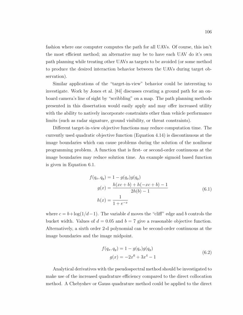
106
fashion where one computer computes the path for all UAVs. Of course, this isn’t
the most efficient method; an alternative may be to have each UAV do it’s own
path planning while treating other UAVs as targets to be avoided (or some method
to produce the desired interaction behavior between the UAVs during target ob-
servation).
Similar applications of the “target-in-view” behavior could be interesting to
investigate. Work by Jones et al. [84] discusses creating a ground path for an on-
board camera’s line of sight by “scribbling” on a map. The path planning methods
presented in this dissertation would easily apply and may offer increased utility
with the ability to natively incorporate constraints other than vehicle performance
limits (such as radar signature, ground visibility, or threat constraints).
Different target-in-view objective functions may reduce computation time. The
currently used quadratic objective function (Equation 4.14) is discontinuous at the
image boundaries which can cause problems during the solution of the nonlinear
programming problem. A function that is first- or second-order continuous at the
image boundaries may reduce solution time. An example sigmoid based function
is given in Equation 6.1.
f(qx, qy) = 1− g(qx)g(qy)
g(x) =ℎ(xc+ b) + ℎ(−xc+ b)− 1
2ℎ(b)− 1
ℎ(x) =1
1 + e−x
(6.1)
where c = b+log(1/d−1). The variable d moves the “cliff” edge and b controls the
bucket width. Values of d = 0.05 and b = 7 give a reasonable objective function.
Alternatively, a sixth order 2-d polynomial can be second-order continuous at the
image boundaries and the image midpoint.
f(qx, qy) = 1− g(qx)g(qy)
g(x) = −2x6 + 3x4 − 1(6.2)
Analytical derivatives with the pseudospectral method should be investigated to
make use of the increased quadrature efficiency compared to the direct collocation
method. A Chebyshev or Gauss quadrature method could be applied to the direct
107
collocation method to produce a less biased comparison between the two methods.
In addition, a constant pitch angle should be incorporated in to the target-in-view
function to account for aircraft pitch in level flight. From here, a gimbaled camera
(time dependent camera orientation) would be useful. Work by Rysdyk [85] on
path following with a gimbaled camera may be useful. Additional constraints such
as landing gear or empennage obstructions could be added to the optimization to
automatically account for various airframes.
A disadvantage of the neural network approximation method is that it currently
only works with problems where final time is fixed. In order to be more useful,
the method needs to be expanded to accommodate problems with free final time.
A method to do this is outlined below. Consider the brachistochrone problem. If
the problem is discretized in terms of horizontal position (since both initial and
final time are given), the neural network method can be applied. Two different
approaches could be taken. The first is to train a network to output ΔVi, Δyi, and
Δ�i that drives the bead from xi to xi+1 given Vi, �i, and a timestep dti. Then
the varied parameters in the optimization problem are the timesteps required to
arrive at the horizontal position at the end of each segment.
The second method is similar, but the network inputs are Vi, �i, and �i+1. The
outputs are ΔVi, Δyi, and the required timestep to arrive at xi+1 from xi. This
formulation is closer to the original problem in that the varied parameters are only
the controls.
These formulations suffer from the limitation in initial and final horizontal
position. If a new final position is chosen, the network needs to be retrained.
However, there may be leeway if the dynamics network is trained over a range
of dt and thus it could handle arbitrary changes in final positions provided an
adequate number of nodes are still used. With this, the number of nodes required
would depend on the range of dt that the network is trained with.
Appendix AAnalytical Derivations for the Direct
Collocation Method
The analytical derivatives and integrals for the direct collocation method are de-
rived here. These derivatives include both the objective and constraint equations
in terms of the hermite approximating polynomials and the equations of motion.
The control and distance-to-target analytical integrations are also derived here.
Recall the Hermite interpolating poynomial equations (Equation 2.4)
xpi(s) = [2(xi − xi+1) + xi + xi+1]s3 (A.1)
+ [3(xi+1 − xi)− 2xi − xi+1]s2
+ xis+ xi
upi(s) = ui + (ui+1 − ui)s (A.2)
where s is nondimentional segment time, s = (t − ti)/�, s ∈ [0, 1]. The length of
the segment in time is � . Note that all dotted ( ˙[⋅]) variables are multiplied by � .
The state equations are repeated below.
x = xu1 = Vt cos( )− VwindN (A.3)
y = xu2 = Vt sin( )− VwindE (A.4)
Vt = xu3 = ul (A.5)
= xu4 = g tan(u�)/Vt (A.6)
109
xt = xt1 = VtgtN (A.7)
yt = xt2 = VtgtE (A.8)
A.1 Integrated control cost
The squared control cost integration is straightforward due to the assumption of
linear behavior over the segment. The basic equation for the itℎ segment is:∫ 1
0
((ui+1 − ui)s� + u0)2 =
�
3
(u2i + uiui+1 + u2i+1
)(A.9)
The partial with respect to ui is then
∂
∂ui=�
3(2ui + ui+1) (A.10)
Note that when forming the derivatives over all the segments, each segment deriva-
tive depends on both the leading and trailing point (except the endpoints).
A.2 Integrated distance-to-target cost
The integration of the distance between the UAV and target over the horizon
time is derived here. The squared distance is used to avoid requiring a square
root operation. Refer to Section 4.1 for variable names. Note that because a
two-dimensional approximation is used, UAV altitude ℎ is constant.
d2 = d2xy + ℎ2 = (x(t)− xt(t))2 + (y(t)− yt(t))2 + ℎ2 (A.11)
Since the true states are only tracked at individual nodes, the Hermite interpolating
polynomials are used as the continuous time history of the states for the integration.
Note that this is the continuous time history over the itℎ segment only.
x(s)i = [2(xi − xi+1) + xi + xi+1]s3
+ [3(xi+1 − xi)− 2xi − xi+1]s2
+ xis+ xi
(A.12)

110
Similar equations are used for y, xt, and yt. Several intermediate variables are
now adopted to simplify notation. These conflict with previously defined notation
and are only used in the context of the remainder of this section. For additional
simplicity, the i notation is dropped and the derivation is given for the first segment:
i = 0. Define a, b, c, d, e, f , g, ℎ:
a = 2
([x0
y0
]−
[x1
y1
])+
[x0
y0
]+
[x1
y1
](A.13)
b = 3
([x1
y1
]−
[x0
y0
])− 2
[x0
y0
]−
[x1
y1
](A.14)
c =
[x0
y0
](A.15)
d =
[x0
y0
](A.16)
e = 2
([xt0
yt0
]−
[xt1
yt1
])+
[xt0
yt0
]+
[xt1
yt1
](A.17)
f = 3
([xt1
yt1
]−
[xt0
yt0
])− 2
[xt0
yt0
]−
[xt1
yt1
](A.18)
g =
[xt0
yt0
](A.19)
ℎ =
[xt0
yt0
](A.20)
Performing the appropriate substitutions, converting Equation A.11 to vector form,
and integrating results in:∫ 1
0
d2xyds =
∫ 1
0
[(a− e)s3 + (b− f)s2 + (c− g)s+ (d− ℎ)
]2ds (A.21)

111
After expanding the squared term, integrating over s ∈ [0, 1], and simplifying the
resulting 7tℎ order polynomial, the result is∫ 1
0
d2xyds =1
7(a− e)2 +
1
3(a− e)(b− f)
+1
5
[(b− f)2 + 2(a− e)(c− g)
]+
1
2[(b− f)(c− g) + (a− e)(d− ℎ)]
+1
3
[(c− g)2 + 2(b− f)(d− ℎ)
]+ (d− ℎ)(c− g) + (d− ℎ)2
(A.22)
And the final distance to target cost is (here ℎ is altitude):
Jdist =
nseg∑i=0
d2xyi + ℎ2 (A.23)
The gradient of the above integration is now derived. The gradient must be
computed for the North and East directions. The following is the general derivative
of Jdist where [⋅] is any variable.
∂Jdist∂[⋅]
=2
7
∂(a− e)∂[⋅]
(a− e)
+1
3
[(b− f)
∂(a− e)∂[⋅]
+ (a− e)∂(b− f)
∂[⋅]
]+
2
5
[(a− e)∂(c− g)
∂[⋅]+ (c− g)
∂(a− e)∂[⋅]
+ (b− f)∂(b− f)
∂[⋅]
]+
1
2
[(b− f)
∂(c− g)
∂[⋅]+ (c− g)
∂(b− f)
∂[⋅]+ (a− e)∂(d− ℎ)
∂[⋅]+ (d− ℎ)
∂(a− e)∂[⋅]
]+
2
3
[(c− g)
∂(c− g)
∂[⋅]+ (b− f)
∂(d− ℎ)
∂[⋅]+ (d− ℎ)
∂(b− f)
∂[⋅]
]+ (d− ℎ)
∂(c− g)
∂[⋅]+ (c− g)
∂(d− ℎ)
∂[⋅]
+ 2(d− ℎ)∂(d− ℎ)
∂[⋅](A.24)
The partials with respect to the states and controls are computed below and sub-
stituted into Equation A.24. The gradient for one segment is determined by the
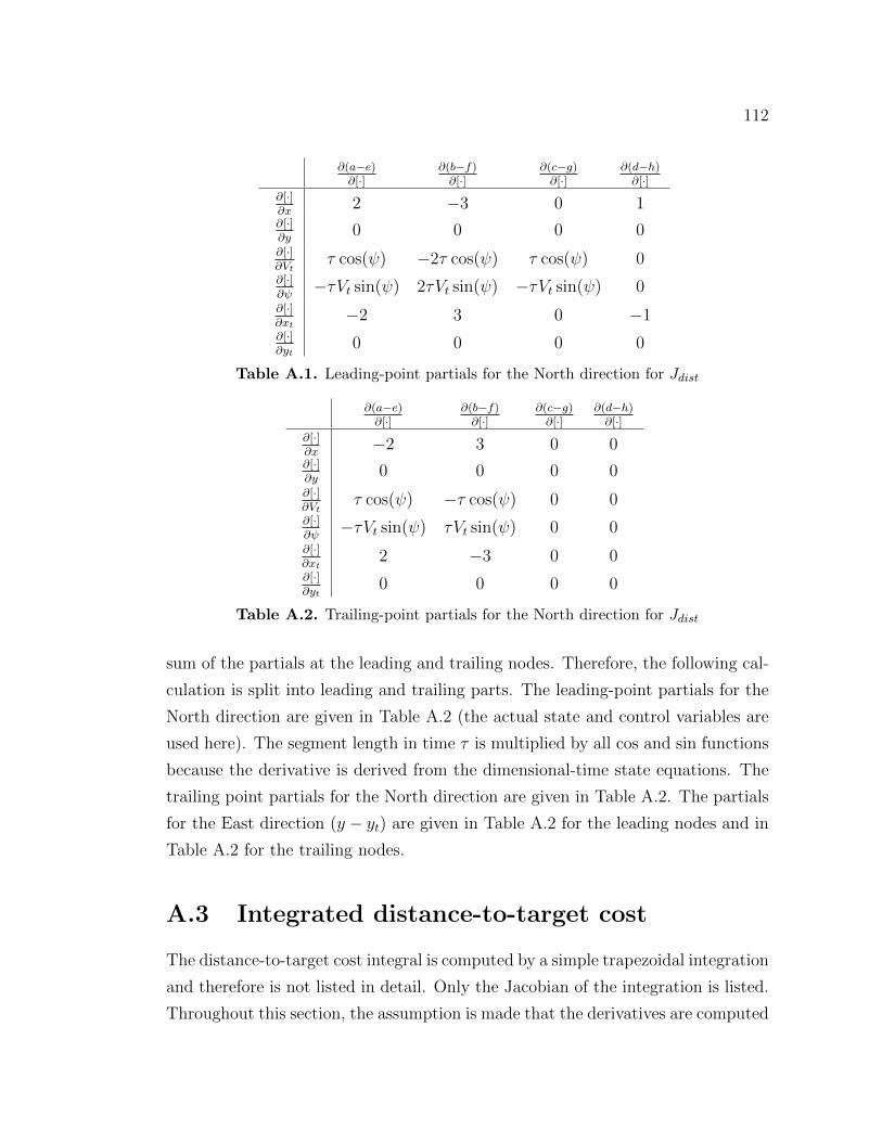
112
∂(a−e)∂[⋅]
∂(b−f)∂[⋅]
∂(c−g)∂[⋅]
∂(d−ℎ)∂[⋅]
∂[⋅]∂x
2 −3 0 1∂[⋅]∂y
0 0 0 0∂[⋅]∂Vt
� cos( ) −2� cos( ) � cos( ) 0∂[⋅]∂
−�Vt sin( ) 2�Vt sin( ) −�Vt sin( ) 0∂[⋅]∂xt
−2 3 0 −1∂[⋅]∂yt
0 0 0 0
Table A.1. Leading-point partials for the North direction for Jdist
∂(a−e)∂[⋅]
∂(b−f)∂[⋅]
∂(c−g)∂[⋅]
∂(d−ℎ)∂[⋅]
∂[⋅]∂x
−2 3 0 0∂[⋅]∂y
0 0 0 0∂[⋅]∂Vt
� cos( ) −� cos( ) 0 0∂[⋅]∂
−�Vt sin( ) �Vt sin( ) 0 0∂[⋅]∂xt
2 −3 0 0∂[⋅]∂yt
0 0 0 0
Table A.2. Trailing-point partials for the North direction for Jdist
sum of the partials at the leading and trailing nodes. Therefore, the following cal-
culation is split into leading and trailing parts. The leading-point partials for the
North direction are given in Table A.2 (the actual state and control variables are
used here). The segment length in time � is multiplied by all cos and sin functions
because the derivative is derived from the dimensional-time state equations. The
trailing point partials for the North direction are given in Table A.2. The partials
for the East direction (y − yt) are given in Table A.2 for the leading nodes and in
Table A.2 for the trailing nodes.
A.3 Integrated distance-to-target cost
The distance-to-target cost integral is computed by a simple trapezoidal integration
and therefore is not listed in detail. Only the Jacobian of the integration is listed.
Throughout this section, the assumption is made that the derivatives are computed

113
∂(a−e)∂[⋅]
∂(b−f)∂[⋅]
∂(c−g)∂[⋅]
∂(d−ℎ)∂[⋅]
∂[⋅]∂x
0 0 0 0∂[⋅]∂y
2 −3 0 1∂[⋅]∂Vt
� sin( ) −2� sin( ) � sin( ) 0∂[⋅]∂
�Vt cos( ) −2�Vt cos( ) �Vt cos( ) 0∂[⋅]∂xt
0 0 0 0∂[⋅]∂yt
−2 3 0 −1
Table A.3. Leading-point partials for the East direction for Jdist
∂(a−e)∂[⋅]
∂(b−f)∂[⋅]
∂(c−g)∂[⋅]
∂(d−ℎ)∂[⋅]
∂[⋅]∂x
0 0 0 0∂[⋅]∂y
−2 3 0 0∂[⋅]∂Vt
� sin( ) −� sin( ) 0 0∂[⋅]∂
�Vt cos( ) −�Vt cos( ) 0 0∂[⋅]∂xt
0 0 0 0∂[⋅]∂yt
2 −3 0 0
Table A.4. Trailing-point partials for the East direction for Jdist
for a particular point along a segment. The chain rule is then used to apply the
derivatives to the trapezoidal integration. At any point along the segment, the
derivatives are affected by the state and control values and the leading and trailing
nodes.
Referring to Equation A.2, we write xi = xpuav(s)−xptgt(s) and yi = ypuav(s)−yptgt(s). This is the relative North and East position pi of the UAV with respect to
the target in terms of the approximating polynomials evaluated at s. Note that the
z component of pi is constant due to the assumption of planar UAV motion and
can be neglected. Taking partial derivatives of xi and yi with respect to the states
and controls, we come across several repeated constants. If we are computing the
contribution to the derivatives of a point with respect to the leading node, the
114
constants are
ta = (s− 1)2(1 + 2s)
tb = (s− 1)2s
tc = 1− s
(A.25)
For the points’s trailing node, we have
ta = s2(3− 2s)
tb = s2(s− 1)
tc = s
(A.26)
The direction cosine matrix at s is defined.
Ri =
⎡⎢⎢⎣c i s i 0
−cu�is i cu�ic i su�isu�is i −su�ic i cu�i
⎤⎥⎥⎦ (A.27)
The gradient of pi with respect to the states and controls is
∂pi∂x
= [ta 0 0] (A.28)
∂pi∂y
= [0 ta 0] (A.29)
∂pi∂Vt
= �tb[c s 0] (A.30)
∂pi∂
= �tbVt[−s c 0] (A.31)
∂pi∂xt
= [−ta 0 0] (A.32)
∂pi∂yt
= [0 −ta 0] (A.33)
∂pi∂ua
= [0 0 0] (A.34)
∂pi∂u�
= [0 0 0] (A.35)
(A.36)
115
Next, the partials of the direction cosine matrix R are given. Note that Ri is
computed from the interpolated i and u�i, not the endpoint values. Recall the
state equations (Eq. A.8) are present in the approximating polynomials (Eq. A.2)
which are used to compute i and u�i. All of these must be accounted for. The
final result in matrix form is
∂Ri
∂x= 0 (A.37)
∂Ri
∂y= 0 (A.38)
∂Ri
∂Vt= −�tb
d idRi
g tan(�)/V 2t (A.39)
∂Ri
∂ =du�idRi
tc +d idRi
g(1/ cos(pℎi))2/Vttb� (A.40)
∂Ri
∂xt= 0 (A.41)
∂Ri
∂yt= 0 (A.42)
∂Ri
∂ua= 0 (A.43)
∂Ri
∂u�=d idRi
ta (A.44)
(A.45)
Next, the derivatives of Ripi are computed with the chain rule. Take note of the
zero valued partials for Ri above.
∂Ripi∂x
= Ri∂Ri
∂x(A.46)
∂Ripi∂y
= Ri∂Ri
∂y(A.47)
∂Ripi∂Vt
= Ri∂Ri
∂Vt+∂Ri
∂Vtpi (A.48)
∂Ripi∂
= Ri∂Ri
∂x+∂Ri
∂ pi (A.49)
∂Ripi∂xt
= −∂Ripi∂x
(A.50)
∂Ripi∂yt
= −∂Ripi∂y
(A.51)
116
∂Ripi∂ua
= 0 (A.52)
∂Ripi∂u�
= Ri∂pi∂u�
+∂Ri
∂u�pi (A.53)
(A.54)
Now the derivatives for T are computed (recall T is defined in Equation 4.9).
∂Ti∂x
=[03×2 −∂Ripi
∂x
](A.55)
∂Ti∂y
=[03×2 −∂Ripi
∂y
](A.56)
∂Ti∂Vt
=[∂Ri∂Vt [:,1:2]
−∂Ripi∂Vt
](A.57)
∂Ti∂
=[∂Ri∂ [:,1:2]
−∂Ripi∂
](A.58)
∂Ti∂xt
=[03×2 −∂Ripi
∂xt
](A.59)
∂Ti∂yt
=[03×2 −∂Ripi
∂yt
](A.60)
∂Ti∂ua
= 0 (A.61)
∂Ti∂u�
=[∂Ri∂u� [:,1:2]
∂Ripi∂u�
](A.62)
(A.63)
Note that ∂Ri∂Vt [:,1:2]
means to extract all of the rows and the first two columns. Fol-
lowing the homography computation in Equation 4.10, the derivatives of KCmTipi
are computed.
∂KCTipi∂x
= KCm
(Ti∂pi∂x
+∂Ti∂xpi
)(A.64)
∂KCTipi∂y
= KCm
(Ti∂pi∂y
+∂Ti∂ypi
)(A.65)
∂KCTipi∂Vt
= KCm
(Ti∂pi∂Vt
+∂Ti∂Vt
pi
)(A.66)
∂KCTipi∂
= KCm
(Ti∂pi∂
+∂Ti∂ pi
)(A.67)
117
∂KCTipi∂xt
= KCm
(Ti∂pi∂xt
+∂Ti∂xt
pi
)(A.68)
∂KCTipi∂yt
= KCm
(Ti∂pi∂yt
+∂Ti∂ytpi
)(A.69)
∂KCTipi∂ua
= 0 (A.70)
∂KCTipi∂u�
= KCm
(Ti∂pi∂u�
+∂Ti∂u�
pi
)(A.71)
(A.72)
The gradient matrix for the unnormalized pixel location derivatives ∇DP , is a row
vector assembled from above eight equations. Continuing with Equation 4.11 and
using the quotient rule,the normalized pixel location derivatives are given by
∇P =
(∇DP[1:2,:]qz − [qx qy]
T∇DP[3,:]
)q2z
(A.73)
where q = [qx qy qz]T is defined in Equation 4.10. Now the final gradient is
assembled. This step applies the chain rule to compute the effect of the pixel
location objective function on the pixel location derivatives (Jtiv = min(q ⋅ q, 1)).
∇JtivP = 2∇P Tq (A.74)
This final gradient is multiplied by the target-in-view weight, � , and a factor of
0.5 if it is computed directly at a node. It is then summed appropriately with the
overall gradient.
A.4 Constraint Derivatives
The collocation constraints for the direct collocation method are given by the
difference between the state equations evaluated at the midpoint of a segment xci
and the derivative of the Hermite cubic polynomial at the midpoint. The relevant
equations are as follows (Refer to Section 2.2).
xci = xpi(0.5) =1
2(xi + xi+1) +
�
8(xi − xi+1) (A.75)
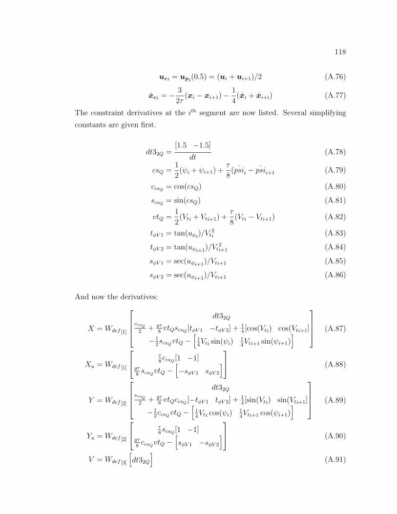
118
uci = upi(0.5) = (ui + ui+1)/2 (A.76)
xci = − 3
2�(xi − xi+1)−
1
4(xi + xi+i) (A.77)
The constraint derivatives at the itℎ segment are now listed. Several simplifying
constants are given first.
dt32Q =[1.5 −1.5]
dt(A.78)
csQ =1
2( i + i+1) +
�
8( ˙psii − ˙psii+1 (A.79)
ccsQ = cos(csQ) (A.80)
scsQ = sin(csQ) (A.81)
vtQ =1
2(Vti + Vti+1) +
�
8(Vti − Vti+1) (A.82)
t�V 1 = tan(u�i)/Vt2i (A.83)
t�V 2 = tan(u�i+1)/Vt2i+1 (A.84)
s�V 1 = sec(u�i+1)/Vti+1 (A.85)
s�V 2 = sec(u�i+1)/Vti+1 (A.86)
And now the derivatives:
X = Wdef [1]
⎡⎢⎢⎣dt32Q
ccsQ2
+ g�8vtQscsQ [t�V 1 −t�V 2] + 1
4[cos(Vti) cos(Vti+1]
−12scsQvtQ −
[14Vti sin( i)
14Vti+1 sin( i+1)
]⎤⎥⎥⎦ (A.87)
Xu = Wdef [1]
⎡⎣ �8ccsQ [1 −1]
g�8scsQvtQ −
[−s�V 1 s�V 2
]⎤⎦ (A.88)
Y = Wdef [2]
⎡⎢⎢⎣dt32Q
scsQ2
+ g�8vtQccsQ [−t�V 1 t�V 2] + 1
4[sin(Vti) sin(Vti+1]
−12ccsQvtQ −
[14Vti cos( i)
14Vti+1 cos( i+1)
]⎤⎥⎥⎦ (A.89)
Yu = Wdef [2]
⎡⎣ �8scsQ [1 −1]
g�8ccsQvtQ −
[s�V 1 −s�V 2
]⎤⎦ (A.90)
V = Wdef [3]
[dt32Q
](A.91)

119
Vu = Wdef [3]
[34
34
](A.92)
Ψ = Wdef [4]
⎡⎣−g2
tan(u�c)/vt2Q −
g4
[t�V 1 t�V 2
]dt32Q
⎤⎦ (A.93)
Ψu = Wdef [4]
⎡⎣ g�8
tan(u�c)/vt2Q
[−1 1
]g2
sec2(u�c)/vtQ
[1 1
]+ g
4
[s�V 1 s�V 2
]dt32Q
⎤⎦ (A.94)
Xt = Wdef [5]dt32Q (A.95)
Yt = Wdef [6]dt32Q (A.96)
The constraint derivatives for the itℎ segment are then assembled columnwise in
the order they appear above into the itℎ column of the constraint Jacobian.
Appendix BNeural Network Weights, Biases,
and Scaling for the UAV Surveillance
Problem
The weights and biases of the three networks used in the UAV surveillance problem
are examined here. Their numerical values are tabulated and the corresponding
Hinton graph is shown with each table. The Hinton graph shows the relative
magnitudes of the weights and biases in a graphical format. Positive weights are
green and negative weights are red. The bias column is highlighted in blue. The
Hinton graph is created by calling the MATLAB command hintonwb(W,b) with
the corresponding weight matrix and bias vector. Each network has three layers
with 15 nodes in the input and hidden layers and the appropriate number of nodes
in the output layer.
B.1 Dynamics Network
The weights and biases for the dynamics network are shown in Tables B.1, B.2,
and B.3. The Hinton graph for the input layer, shown in Figure B.1 shows that
the weight and bias magnitudes are relatively well distributed. Layer 2 and layer
3, shown in Figures B.2 and B.3 respectively, show similar distribution. However,
looking more closely at layer 2, one can see that input 11 does not greatly contribute
to the layer’s output. Thus, a neuron can probably be removed from the input

121
layer.
0 1 2 3 4 5 6
2
4
6
8
10
12
14
Input
Neu
ron
Figure B.1. Dynamics network, Layer 1
0 5 10 15
2
4
6
8
10
12
14
Input
Neu
ron
Figure B.2. Dynamics network, Layer 2

122
0 5 10 15
1
2
3
4
Input
Neu
ron
Figure B.3. Dynamics network, Layer 3
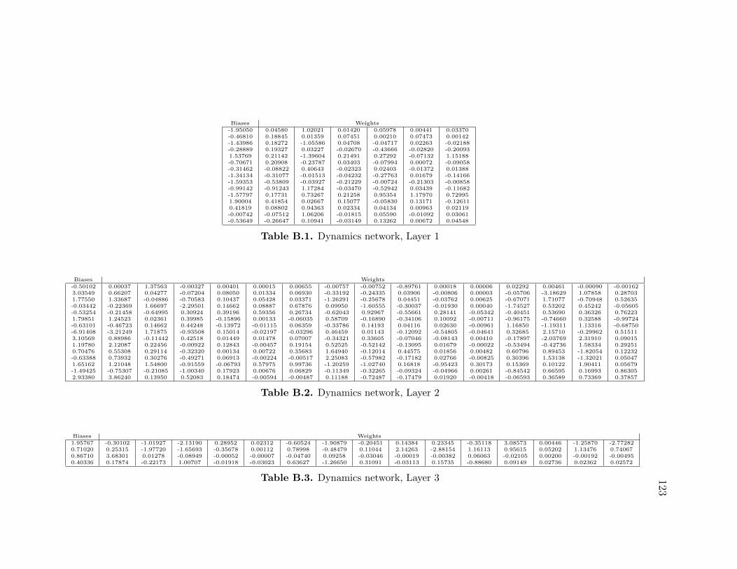
123
Biases Weights-1.95050 0.04580 1.02021 0.01420 0.05978 0.00441 0.03370-0.46810 0.18845 0.01359 0.07451 0.00210 0.07473 0.00142-1.43986 0.18272 -1.05586 0.04708 -0.04717 0.02263 -0.02188-0.28889 0.19327 0.03227 -0.02670 -0.43666 -0.02820 -0.200931.53769 0.21142 -1.39604 0.21491 0.27292 -0.07132 1.15188-0.70671 0.20908 -0.23787 0.03403 -0.07994 0.00072 -0.09058-0.31462 -0.08822 0.40643 -0.02323 0.02403 -0.01372 0.01388-1.34134 -0.31077 -0.01513 -0.04232 -0.27763 0.01679 -0.14166-1.59353 -0.53809 -0.03927 -0.21229 -0.00724 -0.21303 -0.00858-0.99142 -0.91243 1.17284 -0.03470 -0.52942 0.03439 -0.11682-1.57797 0.17731 0.73267 0.21258 0.95354 1.17970 0.729951.90004 0.41854 0.02667 0.15077 -0.05830 0.13171 -0.126110.41819 0.08802 0.94363 0.02334 0.04134 0.00963 0.02119-0.00742 -0.07512 1.06206 -0.01815 0.05590 -0.01092 0.03061-0.53649 -0.26647 0.10941 -0.03149 0.13262 0.00672 0.04548
Table B.1. Dynamics network, Layer 1
Biases Weights-0.50102 0.00037 1.37563 -0.00327 0.00401 0.00015 0.00655 -0.00757 -0.00752 -0.89761 0.00018 0.00006 0.02292 0.00461 -0.00090 -0.001623.03549 0.66207 0.04277 -0.07204 0.08050 0.01334 0.06930 -0.33192 -0.24335 0.03906 -0.00806 0.00003 -0.05706 -3.18629 1.07858 0.287031.77550 1.33687 -0.04886 -0.70583 0.10437 0.05428 0.03371 -1.26291 -0.25678 0.04451 -0.03762 0.00625 -0.67071 1.71077 -0.70948 0.52635-0.03442 -0.22369 1.66697 -2.29501 0.14662 0.08887 0.67876 0.09950 -1.60555 -0.30037 -0.01930 0.00040 -1.74527 0.53202 0.45242 -0.05605-0.53254 -0.21458 -0.64995 0.30924 0.39196 0.59356 0.26734 -0.62043 0.92967 -0.55661 0.28141 -0.05342 -0.40451 0.53690 0.36326 0.762231.79851 1.24523 0.02361 0.39985 -0.15896 0.00133 -0.06035 0.58709 -0.16890 -0.34106 0.10092 -0.00711 -0.96175 -0.74660 0.32588 -0.99724-0.63101 -0.46723 0.14662 0.44248 -0.13972 -0.01115 0.06359 -0.33786 0.14193 0.04116 0.02630 -0.00961 1.16850 -1.19311 1.13316 -0.68750-6.91408 -3.21249 1.71875 -0.93508 0.15014 -0.02197 -0.03296 0.46459 0.01143 -0.12092 -0.54805 -0.04641 0.32685 2.15710 -0.29962 0.515113.10569 0.88986 -0.11442 0.42518 0.01449 0.01478 0.07007 -0.34321 0.33605 -0.07046 -0.08143 0.00410 -0.17897 -2.03769 2.31910 0.090151.19780 2.12087 0.22456 -0.00922 0.12843 -0.00457 0.19154 0.52525 -0.52142 -0.13095 0.01679 -0.00022 -0.53494 -0.42736 1.58334 0.292510.70476 0.55308 0.29114 -0.32320 0.00134 0.00722 0.35683 1.64940 -0.12014 0.44575 0.01856 0.00482 0.60796 0.89453 -1.82054 0.12232-0.63388 0.73932 0.30276 -0.49271 0.06913 -0.00224 -0.00517 2.25083 -0.57982 -0.17182 0.02766 -0.00825 0.30396 1.53138 -1.32021 0.050471.65162 1.21048 1.54800 -0.91559 -0.06793 0.57975 0.99736 -1.20259 -1.02740 0.16818 -0.95423 0.30173 0.15369 0.10122 1.90411 0.05679-1.49425 -0.75307 -0.21085 -1.00340 0.17923 0.00676 0.06829 -0.11349 -0.32265 -0.09324 -0.04966 0.00261 -0.84542 0.66595 0.16993 0.863052.93380 3.86240 0.13950 0.52083 0.18474 -0.00594 -0.00487 0.11188 -0.72487 -0.17479 0.01920 -0.00418 -0.06593 0.36589 0.73369 0.37857
Table B.2. Dynamics network, Layer 2
Biases Weights1.95767 -0.30102 -1.01927 -2.13190 0.28952 0.02312 -0.60524 -1.90879 -0.20451 0.14384 0.23345 -0.35118 3.08573 0.00446 -1.25870 -2.772820.71020 0.25315 -1.97720 -1.65693 -0.35678 0.00112 0.78998 -0.48479 0.11044 2.14263 -2.88154 1.16113 0.95615 0.05202 1.13476 0.740670.86710 3.68301 0.01278 -0.08949 -0.00052 -0.00007 -0.04740 0.09258 -0.03046 -0.00019 -0.00382 0.06063 -0.02105 0.00200 -0.00192 -0.004950.40336 0.17874 -0.22173 1.00707 -0.01918 -0.03023 0.63627 -1.26650 0.31091 -0.03113 0.15735 -0.88680 0.09149 0.02736 0.02362 0.02572
Table B.3. Dynamics network, Layer 3

124
B.2 Distance-to-target Network
The weights and biases for the distance-to-target objective function network are
shown in Tables B.4, B.5, and B.6. The Hinton graphs for each layer are shown
in Figures B.4, B.5, and B.6. The graphs show that the number of neurons for
the distance-to-target objective function can likely be reduced. Looking at layers
2 and 3, the network can probably be reduced by 6 neurons in both layers.
0 1 2 3 4 5 6 7 8
2
4
6
8
10
12
14
Input
Neu
ron
Figure B.4. Distance-to-target network, Layer 1
0 5 10 15
2
4
6
8
10
12
14
Input
Neu
ron
Figure B.5. Distance-to-target network, Layer 2
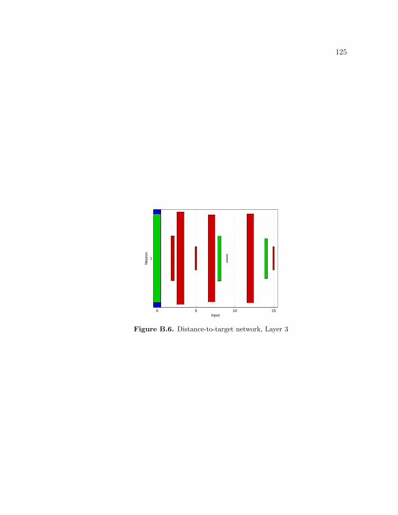
125
0 5 10 15
1
Input
Neu
ron
Figure B.6. Distance-to-target network, Layer 3

126
Biases Weights-0.21604 0.01021 -0.80957 -0.02148 0.16408 0.00216 -0.03347 0.00067 -0.010910.64745 -0.00489 0.00728 -0.29575 -0.03792 -0.00093 -0.00024 -0.00025 -0.00008-0.85100 0.01717 -0.12999 -0.25001 -0.05649 0.00320 -0.00420 0.00063 -0.00149-0.82760 -0.01757 0.01677 -0.20956 0.31066 -0.00338 0.00047 -0.00097 0.00019-0.09095 -0.07965 0.90071 -0.06412 -0.14691 -0.01582 0.03729 -0.00520 0.01236-0.73059 1.93649 1.24505 0.42567 0.38716 1.46265 -1.54761 0.29374 2.60077-0.79105 0.23476 1.52629 0.03478 0.08422 0.04484 0.07057 0.01303 0.02417-0.09071 0.10557 -1.09191 -0.10725 -0.01950 0.02101 -0.04352 0.00663 -0.01463-0.19809 -0.10993 -1.03452 -0.04221 0.00314 -0.02174 -0.04076 -0.00734 -0.01355-0.98365 -1.12803 0.46786 -0.67641 -0.15201 -0.23007 0.01249 -0.08655 0.007540.19887 -0.00482 0.52938 0.10778 0.02377 -0.00110 0.02032 -0.00011 0.00672-1.02782 0.01179 1.16952 -0.12451 0.19418 0.00183 0.05269 -0.00024 0.017450.76696 0.01327 0.05358 0.10529 0.41681 0.00253 0.00268 0.00059 0.000950.06302 0.07590 -0.37126 0.07729 0.06284 0.01518 -0.01650 0.00498 -0.00540-3.07710 -0.18887 -0.14669 0.13089 -0.21223 -0.03980 -0.06629 0.00793 -0.02825
Table B.4. Distance-to-target network, Layer 1
Biases Weights6.02654 6.21419 1.31149 -7.01776 -0.53737 9.72953 0.02481 -4.17193 5.79395 4.99690 -2.20822 -2.73970 0.21796 -3.33029 -8.18893 8.56415-2.05312 -0.88544 0.65995 -2.10290 -0.65018 -1.19889 0.00083 0.39940 0.49710 -1.15177 0.02846 -0.73753 0.16831 -0.35571 -1.33821 -0.08892-4.28725 -0.62118 2.15118 -2.03862 -1.08461 -0.49618 0.00037 -0.14154 -0.07299 0.57300 0.03503 0.67437 0.01409 0.62648 0.67339 -0.54783-4.29740 -0.31306 2.45724 -3.50886 -0.37958 0.83771 -0.01111 0.37526 -0.80829 0.12429 1.24942 -1.11031 -0.96856 3.32235 1.63553 0.35875-14.4555 -3.33537 -5.16914 -6.11492 -6.80354 -2.64027 0.77737 0.40221 2.93421 -5.61342 2.17846 -11.1169 -1.83892 -5.00346 -20.4719 -0.548319.86047 -7.52877 -6.71300 -12.1850 8.16081 -5.86058 -10.3530 -7.44890 0.09184 -2.18166 -6.91767 -2.76799 7.37059 0.56102 7.48807 8.35150-2.15152 0.81064 1.61788 -0.61386 -1.59750 -0.07089 0.00018 0.04913 0.36566 -1.47218 0.00016 -1.63520 -0.51735 1.31879 -2.22167 0.26689-2.19017 -0.98367 2.25310 1.91281 -0.09544 -0.27410 0.00206 -0.51450 0.69856 -1.07475 0.05523 0.65846 0.69104 -0.07039 -0.82603 0.29302-2.54448 -0.91827 1.99120 -0.96928 -0.38283 -0.15807 -0.01191 -1.86748 -1.38306 -1.01511 -0.40382 -1.78047 1.40046 -1.05189 -1.71411 -0.45562-94.2125 -98.5807 -10.5772 -51.1740 8.93134 -36.1670 -3.50859 2.94309 12.0875 3.68274 -16.4505 1.74011 18.1317 78.5243 77.7152 2.456684.97833 -4.62784 -5.32713 -9.68757 12.07112 5.65539 -0.07073 -0.82959 2.59353 0.23049 -0.40254 2.35527 1.15958 -0.08908 2.76469 0.67045-0.84836 -1.08546 1.30590 -0.16839 -1.50783 -0.67384 -0.00036 -0.00252 -0.90807 0.76286 -0.03606 -1.16821 0.57492 1.49927 0.28976 1.33800-11.0818 -3.35417 8.18197 -0.95755 1.00083 -1.43648 -6.04720 3.64350 2.07345 -2.83837 -1.82801 0.36828 -1.65293 -2.74215 -0.84734 -0.902232.96803 3.31911 -0.17682 -1.34545 0.10015 1.54406 0.00078 -0.23198 0.35745 -1.43549 -0.03329 0.55151 1.01221 -0.12210 -3.22391 1.422112.73213 3.38774 0.93391 1.24331 0.29736 0.32177 -0.00134 0.11440 -0.34888 -1.35120 -0.01080 0.11732 0.66880 0.96514 -1.72751 1.13080
Table B.5. Distance-to-target network, Layer 2
Biases Weights2.85086 -0.00077 -0.76264 -3.13470 0.00021 -0.23004 0.00006 -2.78657 0.77351 -0.05751 0.00032 0.00202 -2.89532 -0.00012 0.60677 -0.23087
Table B.6. Distance-to-target network, Layer 3

127
B.3 Target-in-view Network
The weights and biases for the target-in-view objective function network are shown
in Tables B.7, B.8, and B.9. The Hinton graphs for each layer are shown in
Figures B.7, B.8, and B.9. This network shows good distribution of weight and
bias magnitudes except for inputs 1, 5, and 7, which correspond to Vt, ua0 , and
ua1 . This suggests that these inputs could be removed from the network without
affecting network performance. This seems to be an intuitive result, since airspeed
and acceleration command would have a weak effect on the target-in-view objective
function value given the short time step and relatively low speed of the UAV. Note
that this only likely applies is the time step is kept low (this network is trained
over 2 seconds) and the speed capabilities of the UAV are low.
0 1 2 3 4 5 6 7 8
2
4
6
8
10
12
14
Input
Neu
ron
Figure B.7. Target-in-view network, Layer 1
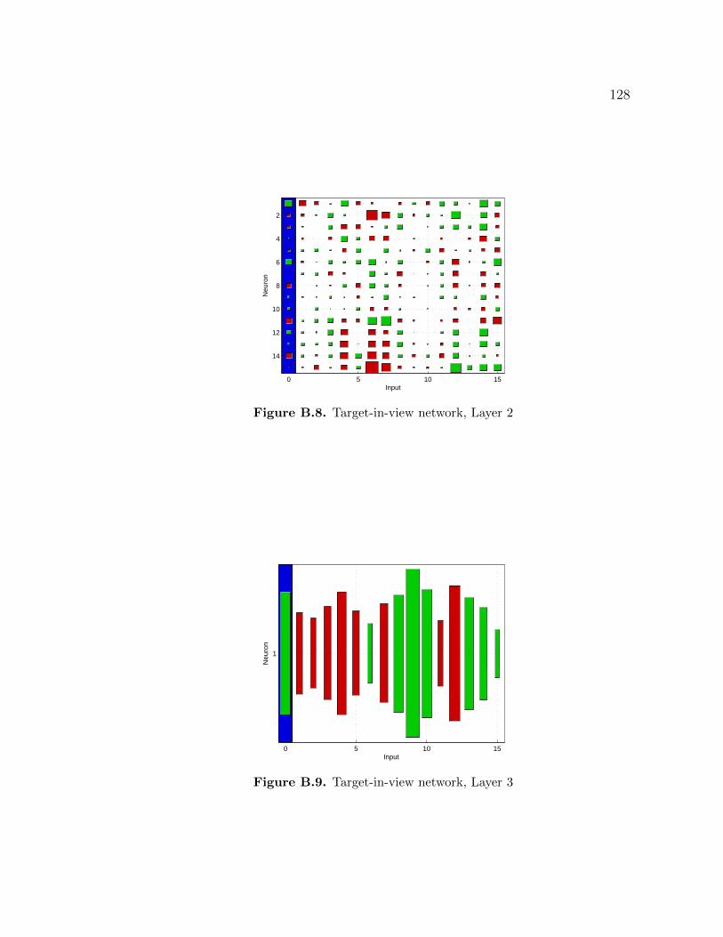
128
0 5 10 15
2
4
6
8
10
12
14
Input
Neu
ron
Figure B.8. Target-in-view network, Layer 2
0 5 10 15
1
Input
Neu
ron
Figure B.9. Target-in-view network, Layer 3

129
Biases Weights-2.94929 0.00099 2.97493 2.20258 0.46950 0.02720 0.00988 -0.02443 0.39630-1.62435 -0.04372 2.21664 2.19293 -0.01861 0.00472 0.22375 -0.00299 -0.47192-0.10427 -0.03775 0.89504 -1.11893 -1.28858 -0.00019 0.28530 -0.00167 0.13035-1.70835 -0.02617 1.75461 0.40810 -0.63221 0.00910 0.16992 -0.01142 0.03850-0.30691 0.00447 1.13484 0.94700 -0.20773 0.00288 -0.06015 0.00425 -0.128510.47374 -0.00427 1.56403 -1.29160 0.13378 0.00719 0.21487 0.00536 0.14038-0.50530 0.02589 -1.65817 0.66334 0.36301 -0.00345 -0.18927 -0.00083 -0.145350.23616 0.05475 -1.57911 0.42698 0.41123 -0.00163 -0.34063 -0.00045 -0.122360.34004 -0.00499 2.38151 -0.31137 -1.95144 0.02450 0.78466 0.03017 -0.61150-1.02013 0.01043 -1.30500 0106046 -1.23123 0.01808 -0.24025 0.02193 0.754990.09557 0.00835 0.01031 -0.07063 0.68188 -0.00235 -0.38194 0.00197 0.107510.39375 0.00930 1.01436 -1.85027 0.72562 0.00459 0.09160 0.00491 0.026010.45142 -0.04694 0.61908 1.77586 -3.32755 -0.00913 -0.19972 -0.00955 0.09565-1.23704 -0.00785 1.32612 1.18290 -0.76564 0.00872 0.12575 -0.00433 -0.00659-0.82476 -0.02324 -0.85710 -0.31270 -0.60536 -0.00430 0.11924 -0.00393 0.07551
Table B.7. Target-in-view network, Layer 1
Biases Weights5.32225 -4.40886 -1.37927 0.30083 4.46147 -1.70876 -0.74100 0.07613 -1.05840 0.84507 -1.48534 2.39150 1.57093 -0.21933 5.80165 2.99864-1.34683 -1.05988 -0.44007 2.39285 0.48910 -0.01149 -11.6312 -6.20986 2.45461 -0.72438 1.05303 0.43045 7.11524 -0.00756 4.00208 -2.01784-1.16270 -0.40628 0.08956 1.78201 -3.19652 -2.05236 -0.45522 0.85116 2.52106 0.04406 -0.18372 1.42964 2.09681 1.02204 5.41985 -1.171920.21467 -0.41706 -0.07217 -0.94831 3.87480 1.32349 -2.22590 -2.51233 0.12752 0.25086 -0.13546 -0.45314 -0.12720 -0.73939 -4.22053 1.92243-0.88910 0.89138 1.26327 0.30598 -1.59481 1.80063 0.10287 1.94043 0.34056 -0.73619 1.71235 -2.03568 0.26571 0.48383 -1.10173 -2.684313.72743 -0.89998 0.24193 1.62738 0.79396 2.48942 4.52526 0.29791 2.35376 -0.16926 -0.87300 1.38180 -4.42239 -0.36291 0.86315 5.443710.12494 0.80481 0.99483 -2.00677 -0.74799 0.08137 3.25625 0.76597 -2.86609 -0.19156 -0.25286 1.00011 -3.24241 -0.06792 -2.37010 0.63546-2.24378 -0.12379 0.31064 -0.44623 1.40350 -2.12601 3.31082 1.47218 -1.07444 0.02204 0.18609 0.90442 -2.20626 -0.28291 -1.74551 -2.884250.65789 -0.50340 -0.25189 0.64765 0.26566 -1.08937 0.51071 2.00465 -0.23539 0.44220 -0.10168 1.31085 0.74745 0.05062 2.37953 -0.891460.87585 -0.00061 0.92716 0.19896 0.23767 1.41348 -1.57819 -1.39816 0.52196 0.04524 -0.19508 -0.01446 -0.83237 -0.59958 -1.63113 1.60596-3.90579 0.36791 1.25678 3.02436 -2.03468 -1.24929 6.33227 9.00597 -1.68149 -0.37664 -0.02265 -0.54657 -2.20386 -0.12670 -3.11504 -6.350951.92545 0.69379 -0.41647 2.86123 -4.52158 0.04839 -4.82774 -2.13031 2.52839 0.21307 -0.00397 0.82466 3.19883 -0.04011 6.39342 0.109140.57206 1.15802 0.51749 1.56908 -5.56576 -0.17512 -5.21831 -4.57954 2.87726 -0.46286 -0.25431 -1.03615 2.72596 0.16115 4.50512 1.60529-3.70679 0.77028 -0.50058 1.09863 -5.40246 3.00634 -6.23524 -4.35755 1.50309 -0.84639 0.92218 -2.39641 3.58317 0.38676 0.77052 -0.65887-0.17863 -0.39211 -2.31623 0.33224 -3.64525 1.43627 -15.9869 -7.81363 -1.28001 -0.40080 -0.54812 0.39449 10.33897 1.94355 5.45472 5.52309
Table B.8. Target-in-view network, Layer 2
Biases Weights22.4634 -10.0144 -7.52627 -13.0326 -22.0967 -10.7190 5.51253 -14.6370 20.2171 41.5256 24.3277 -6.62902 -27.0324 18.6734 12.8679 3.76143
Table B.9. Target-in-view network, Layer 3
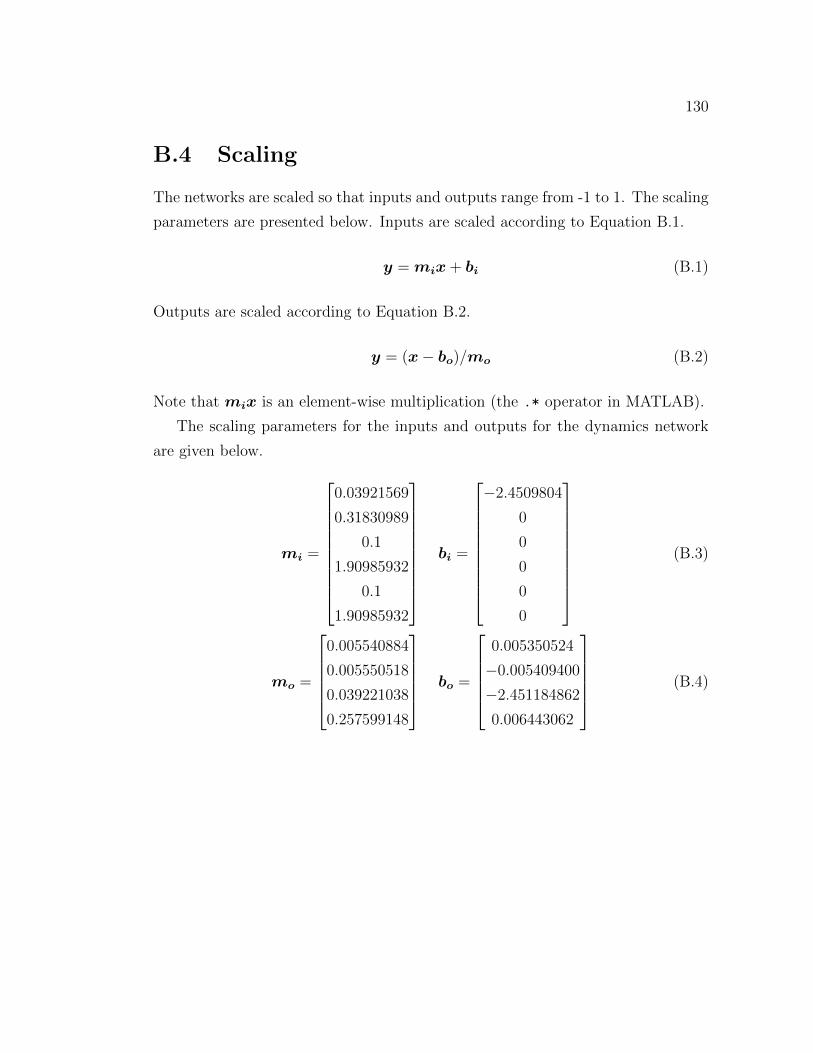
130
B.4 Scaling
The networks are scaled so that inputs and outputs range from -1 to 1. The scaling
parameters are presented below. Inputs are scaled according to Equation B.1.
y = mix+ bi (B.1)
Outputs are scaled according to Equation B.2.
y = (x− bo)/mo (B.2)
Note that mix is an element-wise multiplication (the .* operator in MATLAB).
The scaling parameters for the inputs and outputs for the dynamics network
are given below.
mi =
⎡⎢⎢⎢⎢⎢⎢⎢⎢⎢⎣
0.03921569
0.31830989
0.1
1.90985932
0.1
1.90985932
⎤⎥⎥⎥⎥⎥⎥⎥⎥⎥⎦bi =
⎡⎢⎢⎢⎢⎢⎢⎢⎢⎢⎣
−2.4509804
0
0
0
0
0
⎤⎥⎥⎥⎥⎥⎥⎥⎥⎥⎦(B.3)
mo =
⎡⎢⎢⎢⎢⎣0.005540884
0.005550518
0.039221038
0.257599148
⎤⎥⎥⎥⎥⎦ bo =
⎡⎢⎢⎢⎢⎣0.005350524
−0.005409400
−2.451184862
0.006443062
⎤⎥⎥⎥⎥⎦ (B.4)

131
For the distance-to-target network, the scaling parameters are given below.
mi =
⎡⎢⎢⎢⎢⎢⎢⎢⎢⎢⎢⎢⎢⎢⎢⎣
0.039215686
0.318309886
0.001
0.001
0.1
1.909859317
0.1
1.909859317
⎤⎥⎥⎥⎥⎥⎥⎥⎥⎥⎥⎥⎥⎥⎥⎦bi =
⎡⎢⎢⎢⎢⎢⎢⎢⎢⎢⎢⎢⎢⎢⎢⎣
−2.4509804
0
0
0
0
0
0
0
⎤⎥⎥⎥⎥⎥⎥⎥⎥⎥⎥⎥⎥⎥⎥⎦(B.5)
mo =[4.601430E − 007
]b0 =
[−1.1482193
](B.6)
For the target-in-view objective function network, the scaling parameters are
given below. The input parameters are the same as the distance-to-target network.
mi =
⎡⎢⎢⎢⎢⎢⎢⎢⎢⎢⎢⎢⎢⎢⎢⎣
0.039215686
0.318309886
0.001
0.001
0.1
1.909859317
0.1
1.909859317
⎤⎥⎥⎥⎥⎥⎥⎥⎥⎥⎥⎥⎥⎥⎥⎦bi =
⎡⎢⎢⎢⎢⎢⎢⎢⎢⎢⎢⎢⎢⎢⎢⎣
−2.4509804
0
0
0
0
0
0
0
⎤⎥⎥⎥⎥⎥⎥⎥⎥⎥⎥⎥⎥⎥⎥⎦(B.7)
mo =[0.537292446
]bo =
[−0.074584891
](B.8)
Bibliography
[1] Betts, J. T. (1998) “Survey of numerical methods for trajectory optimiza-tion.” Journal of Guidance, Control, and Dynamics, 21(2), pp. 193–207.
[2] Stengel, R. F. (1986) Optimal Control and Estimation. Dover Publications,Inc., New York.
[3] Dickmanns, E. D. and K. H. Well (1974) “Approximate solution of op-timal control problems using third order hermite polynomial functions.” InProceedings of the IFIP Technical Conference, pp. 158–166. Springer-Verlag,London, UK.
[4] Hargraves, C. R. and S. W. Paris (1987) “Direct trajectory optimizationusing nonlinear programming and collocation.” Journal of Guidance, Control,and Dynamics, 10(4), pp. 338–342.
[5] Enright, P. J. and B. A. Conway (1991) “Optimal finite-thrust space-craft trajectories using collocation and nonlinear programming.” Journal ofGuidance, Control, and Dynamics, 14(5), pp. 981–985.
[6] Roh, W. and Y. Kim (2002) “Trajectory optimization for a multi-stagelaunch vehicle using time finite element and direct collocation methods.” En-gineering Optimization, 34(1), pp. 15–32. doi:10.1080/03052150210912.
[7] Herman, A. L. and B. A. Conway (1996) “Direct optimization using collo-cation based on high-order gauss-lobatto quadrature rules.” Journal of Guid-ance, Control, and Dynamics, 19(3), pp. 592–599.
[8] Coverstone-Carroll, V. and J. E. Prussing (1995) “Optimal cooper-ative power-limited rendezvous with propellant constraints.” Journal of theAstronautical Sciences, 43(3), pp. 289–305.
[9] Tang, S. and B. A. Conway (1995) “Optimization of low-thrust interplan-etary trajectories using collocation and nonlinear programming.” Journal ofGuidance, Control, and Dynamics, 18(3), pp. 599–604.

133
[10] Enright, P. J. and B. A. Conway (1992) “Discrete approximations tooptimal trajectories using direct transcription and nonlinear programming.”Journal of Guidance, Control, and Dynamics, 15(4), pp. 994–1002.
[11] Herman, A. L. and B. A. Conway (1992) “Optimal spacecraft attitudecontrol using collocation and nonlinear programming.” Journal of Guidance,Control, and Dynamics, 15(5), pp. 1287–1289.
[12] Horie, K. and B. A. Conway (1999) “Optimal aeroassisted orbital inter-ception.” Journal of Guidance, Control, and Dynamics, 22(5), pp. 625–631.
[13] Gill, P. E., W. Murray, and M. A. Saunders (2002) “Snopt: An sqpalgorithm for large-scale constrained optimization.” SIAM Journal on Opti-mization, 12(4), pp. 979–1006.
[14] Razzaghi, M. and G. N. Elnagar (1994) “Pseudospectral collocationmethod for the brachistochrone problem.” Mathematics and Computers inSimulation, 36(3), pp. 241–246. doi:10.1016/0378-4754(94)90008-6.
[15] Richards, A. and J. P. How (2002) “Aircraft trajectory planning withcollision avoidance using mixed integer linear programming.” Proceedingsof the American Control Conference, 3, pp. 1936–1941. doi:10.1109/ACC.
2002.1023918.
[16] Holland, J. H. (1975) Adaptation in Natural and Artificial Systems. Uni-versity of Michigan Press, Ann Arbor.
[17] Li, S., R. Mehra, R. Smith, and R. W. Beard (2000) “Multi-spacecrafttrajectory optimization and control using genetic algorithm techniques.” In2000 IEEE Aerospace Conference, volume 7 of IEEE Aerospace ConferenceProceedings, pp. 99–108. IEEE.
[18] Konak, A., D. W. Coit, and A. E. Smith (2006) “Multi-objective opti-mization using genetic algorithms: A tutorial.” Reliability Engineering andSystem Safety, 91(9), pp. 992–1007. doi:10.1016/j.ress.2005.11.018.
[19] Goto, N. and H. Kawable (2000) “Direct optimization methods appliedto a nonlinear optimal control problem.” Mathematics and Computers inSimulation, 51(6), pp. 557–577. doi:10.1016/S0378-4754(99)00145-7.
[20] Zhao, Y. J. (2004) “Optimal patterns of glider dynamic soaring.” OptimalControl Applications and Methods, 25(2), pp. 67–89. doi:10.1002/oca.739.
[21] Zhao, Y. J. and Y. C. Qi (2004) “Minimum fuel powered dynamic soar-ing of unmanned aerial vehicles utilizing wind gradients.” Optimal ControlApplications and Methods, 25(5), pp. 211–233. doi:10.1002/oca.744.

134
[22] Qi, Y. and Y. J. Zhao (2005) “Energy-efficient trajectories of unmannedaerial vehicles flying through thermals.” Journal of Aerospace Engineering,18(2), pp. 84–92. doi:10.1061/(ASCE)0893-1321(2005)18:2(84).
[23] Borrelli, F., D. Subramanian, A. U. Raghunathan, and L. T.Biegler (2006) “Milp and nlp techniques for centralized trajectory plan-ning of multiple unmanned air vehicles.” In American Control Conference,pp. 1–6.
[24] Misovec, K., T. Inanc, J. Wohletz, and R. M. Murray (2003) “Low-observable nonlinear trajectory generation for unmanned air vehicles.” Pro-ceedings of the IEEE Conference on Decision and Control, 3, pp. 3103–3110.doi:10.1109/CDC.2003.1273100.
[25] Milam, M. B., K. Mushambi, and R. M. Murray (2000) “A new compu-tational approach to real-time trajectory generation for constrained mechan-ical systems.” Proceedings of the IEEE Conference on Decision and Control,1, pp. 845–851. doi:10.1109/CDC.2000.912875.
[26] Williams, P. (2007) “Three-dimensional aircraft terrain-following via real-time optimal control.” Journal of Guidance, Control, and Dynamics, 30(4),pp. 1201–1206. doi:10.2514/1.29145.
[27] Yakimenko, O. A., Y. Xu, and G. Basset (2008) “Computing short-timeaircraft maneuvers using direct methods.” In Collection of Technical Papers- AIAA Guidance, Navigation, and Control Conference 2008, volume 1, pp.1–23.
[28] How, J., E. King, and Y. Kuwata (2004) “Flight demonstrations of co-operative control for uav teams.” Collection of Technical Papers - AIAA 3rd”Unmanned-Unlimited” Technical Conference, Workshop, and Exhibit, 1, pp.505–513.
[29] Toupet, O. and B. Mettler (2006) “Design and flight test evaluation ofguidance system for autonomous rotorcraft.” Collection of Technical Papers -AIAA Guidance, Navigation, and Control Conference 2006, 2, pp. 1288–1297.
[30] Flint, M., M. Polycarpou, and E. Fernandez-Gaucherand (2002)“Cooperative control for multiple autonomous uav’s searching for targets.”Proceedings of the IEEE Conference on Decision and Control, 3, pp. 2823–2828. Autonomous unmanned aerial vehicles;Cooperative control;Targetsearching;Discrete time stochastic decision model;. doi:10.1109/CDC.2002.
1184272.

135
[31] Anderson, M. B., J. L. Lopez, and J. H. Evers (2006) “A comparison oftrajectory determination approaches for small uavs.” Collection of TechnicalPapers - 2006 Atmospheric Flight Mechanics Conference, 2, pp. 1345–1356.
[32] Shima, T., S. J. Rasmussen, and A. G. Sparks (2005) “Uav coopera-tive multiple task assignments using genetic algorithms.” Proceedings of theAmerican Control Conference, 5, pp. 2989–2994.
[33] Nikolos, I. K., K. P. Valavanis, N. C. Tsourveloudis, and A. N.Kostaras (2003) “Evolutionary algorithm based offline/online path plannerfor uav navigation.” IEEE Transactions on Systems, Man, and Cybernetics,Part B: Cybernetics, 33(6), pp. 898–912. doi:10.1109/TSMCB.2002.804370.
[34] Stover, J. A. and R. Kumar (1999) “Behavior-based architecture for thedesign of intelligent controllers for autonomous systems.” In IEEE Interna-tional Symposium on Intelligent Control - Proceedings, pp. 308–313.
[35] Miller, J. A., P. D. Minear, A. F. Niessner, Jr., A. M. DeLullo,B. R. Geiger, L. N. Long, and J. F. Horn (2007) “Intelligent unmannedair vehicle flight systems.” Journal of Aerospace Computing, Information andCommunication, 4(5), pp. 816–835.
[36] Sinsley, G. L., J. A. Miller, L. N. Long, B. R. Geiger, A. F. Niess-ner, Jr., and J. F. Horn (2007) “An intelligent controller for collaborativeunmanned air vehicles.” In Proceedings of the 2007 IEEE Symposium on Com-putational Intelligence in Security and Defense Applications, CISDA 2007, pp.139–144. doi:10.1109/CISDA.2007.368146.
[37] Geiger, B. R., J. F. Horn, A. M. DeLullo, L. N. Long, and A. F.Niessner, Jr. (2006) “Optimal path planning of uavs using direct colloca-tion with nonlinear programming.” Collection of Technical Papers - AIAAGuidance, Navigation, and Control Conference 2006, 2, pp. 1257–1269.
[38] Ross, J. A. (2008) Computer vision and target localization algorithms forautonomous Unmanned Aerial Vehicles. Master’s thesis, The PennsylvaniaState University, University Park, PA.
[39] Ross, J. A., B. R. Geiger, G. L. Sinsley, J. F. Horn, L. N. Long,and A. F. Niessner (2008) “Vision-based target geolocation and optimalsurveillance on an unmanned aerial vehicle.” In AIAA Guidance, Navigationand Control Conference and Exhibit, pp. 1–15. AIAA, Honolulu, Hawaii.
[40] Sinsley, G. L., L. N. Long, B. R. Geiger, J. F. Horn, and A. F.Niessner (2009) “Fusion of unmanned aerial vehicle range and vision sen-sors using fuzzy logic and particles.” Collection of Technical Papers - AIAAInfoTech at Aerospace, 1, pp. 1–18.
136
[41] Gottlieb, D. and S. A. Orszag (1977) Numerical Analysis of SpectralMethods: Theory and Application, volume 26. Society for Industrial and Ap-plied Mathematics, Philadelphia, PA, USA.
[42] Gottlieb, D., Y. M. Hussaini, and S. A. Orszag (1984) “Theory andapplications of spectral methods.” In Spectral Methods for Partial Differ-ential Equations, pp. 1–54. Society for Industrial and Applied Mathematics,Philadelphia, PA.
[43] Hussaini, M. Y. and T. A. Zang (1987) “Spectral methods in fluid dy-namics.” Annual Review of Fluid Mechanics, 19(1), pp. 339–367. doi:
10.1146/annurev.fl.19.010187.002011.
[44] Trefethen, L. N. (2000) Spectral Methods in MATLAB. Society for Indus-trial and Applied Mathematics, Philadelphia, PA, USA.
[45] Huntington, G. T., D. A. Benson, and A. V. Rao (2007) “A comparisonof accuracy and computational efficiency of three pseudospectral methods.”In Collection of Technical Papers - AIAA Guidance, Navigation, and ControlConference 2007, volume 1, pp. 840–864.
[46] Fahroo, F. and M. I. Ross (2002) “Direct trajectory optimization by achebyshev pseudospectral method.” Journal of Guidance, Control, and Dy-namics, 25(1), pp. 160–166.
[47] Elnagar, G. N. and M. A. Kazemi (1998) “Pseudospectral chebyshevoptimal control of constrained nonlinear dynamical systems.” Computa-tional Optimization and Applications, 11(2), pp. 195–217. doi:10.1023/A:
1018694111831.
[48] Fahroo, F. and I. M. Ross (2001) “Costate estimation by a legendre pseu-dospectral method.” Journal of Guidance, Control, and Dynamics, 24(2), pp.270–277.
[49] Williams, P. (2004) “Jacobi pseudospectral method for solving optimal con-trol problems.” Journal of Guidance, Control, and Dynamics, 27(2), pp.293–297.
[50] Benson, D. A., G. T. Huntington, T. P. Thorvaldsen, and A. V.Rao (2006) “Direct trajectory optimization and costate estimation via an or-thogonal collocation method.” Journal of Guidance, Control, and Dynamics,29(6), pp. 1435–1440. doi:10.2514/1.20478.
[51] Kameswaran, S. and L. T. Biegler (2008) “Convergence rates for di-rect transcription of optimal control problems using collocation at radau
137
points.” Comput. Optim. Appl., 41(1), pp. 81–126. doi:10.1007/
s10589-007-9098-9.
[52] Clenshaw, C. W. and A. R. Curtis (1960) “A method for numericalintegration on an automatic computer.” Numerische Mathematik, 2(1), pp.197–205. doi:10.1007/BF01386223.
[53] Davis, P. J. and P. Rabinowitz (1975) Methods of Numerical Integration.Academic Press, New York, NY, USA.
[54] Trefethen, L. N. (2008) “Is gauss quadrature better than clenshaw-curtis?”SIAM Rev., 50(1), pp. 67–87. doi:10.1137/060659831.
[55] Benson, D. A. (2008). “Gpops and diagonal d matrix.” Personal emailcorrespondence, 3 Nov 2008.
[56] Meditch, J. (1964) “On the problem of optimal thrust programming fora lunar soft landing.” Automatic Control, IEEE Transactions on, 9(4), pp.477–484.
[57] Yakimenko, O. A. (2000) “Direct method for rapid prototyping of near-optimal aircraft trajectories.” Journal of Guidance, Control, and Dynamics,23(5), pp. 865–875.
[58] Geiger, B. R. and J. F. Horn (2009) “Neural network based trajectoryoptimization for unmanned aerial vehicles.” In 47th AIAA Aerospace SciencesMeeting. AIAA, Orlando, Florida.
[59] Horn, J. F. and B. R. Geiger (2009) “Use of neural network approximationin multiple-unmanned aerial vehicle trajectory optimization.” In To appear inthe AIAA Guidance, Navigation and Control Conference and Exhibit. Chicago,IL.
[60] Rump, S. M. (1999) “INTLAB - INTerval LABoratory.” In T. Csendes,editor, Developments in Reliable Computing, pp. 77–104. Kluwer AcademicPublishers, Dordrecht.
[61] Martins, J. R. R. A., P. Sturdza, and J. J. Alonso (2003) “Thecomplex-step derivative approximation.” ACM Trans. Math. Softw., 29(3),pp. 245–262. doi:10.1145/838250.838251.
[62] Hornik, K., M. Stinchcombe, and H. White (1990) “Universal approx-imation of an unknown mapping and its derivatives using multilayer feed-forward networks.” Neural Networks, 3(5), pp. 551–560. doi:10.1016/
0893-6080(90)90005-6.

138
[63] Gallant A., R. and H. White (1992) “On learning the derivatives of anunknown mapping with multilayer feedforward networks.” Neural Networks,5(1), pp. 129–138.
[64] Leshno, M., V. Y. Lin, A. Pinkus, and S. Schocken (1993) “Multilayerfeedforward networks with a nonpolynomial activation function can approxi-mate any function.” Neural Networks, 6(6), pp. 861–867.
[65] Basson, E. and A. P. Engelbrecht (1999) “Approximation of a functionand its derivatives in feedforward neural networks.” In Proceedings of theInternational Joint Conference on Neural Networks, volume 1, pp. 419–421.doi:10.1109/IJCNN.1999.831531.
[66] Lu, B.-L., H. Kita, and Y. Nishikawa (1999) “Inverting feedforward neuralnetworks using linear and nonlinear programming.” IEEE Transactions onNeural Networks, 10(6), pp. 1271–1290. doi:10.1109/72.809074.
[67] Dennis, J. B. (1959) Mathematical Programming and Electrical Networks.Ph.D. thesis, Massachusetts Institute of Technology. Available from: http:
//hdl.handle.net/1721.1/13366.
[68] Effati, S. and M. Baymani (2005) “A new nonlinear neural network forsolving quadratic programming problems.” Applied Mathematics and Com-putation, 165(3), pp. 719–729. doi:10.1016/j.amc.2004.04.117.
[69] Reifman, J. and E. E. Feldman (1999) “Nonlinear programming withfeedforward neural networks.” In Proceedings of the International Joint Con-ference on Neural Networks, volume 1, pp. 594–598. doi:10.1109/IJCNN.
1999.831565.
[70] Niestroy, M. (1998) “Optimal feedback controller approximation using neu-ral networks and nonlinear programming techniques.” Neural Networks Pro-ceedings, 1998. IEEE World Congress on Computational Intelligence. The1998 IEEE International Joint Conference on, 3, pp. 2110–2115. doi:
10.1109/IJCNN.1998.687185.
[71] Seong, C. Y. and B. Widrow (2001) “Neural dynamic optimization forcontrol systems-part iii: Applications.” IEEE Transactions on Systems, Man,and Cybernetics, Part B: Cybernetics, 31(4), pp. 502–513. doi:10.1109/
3477.938256.
[72] Peng, X., A. Verma, and R. J. Mayer (2007) “Neural dynamic optimiza-tion for autonomous aerial vehicle trajectory design.” In Proceedings of SPIE- The International Society for Optical Engineering, volume 6576, p. 65760.doi:10.1117/12.720126.

139
[73] Yeh, I.-C. (1999) “Design of high-performance concrete mixture using neuralnetworks and nonlinear programming.” Journal of Computing in Civil Engi-neering, 13(1), pp. 36–42. doi:10.1061/(ASCE)0887-3801(1999)13:1(36).
[74] Inanc, T., M. K. Muezzinoglu, K. Misovec, and R. M. Murray (2008)“Framework for low-observable trajectory generation in presence of multipleradars.” Journal of Guidance, Control, and Dynamics, 31(6), pp. 1740–1749.doi:10.2514/1.35287.
[75] Trucco, E. and A. Verri (1998) Introductory Techniques for 3-D ComputerVision. Prentice-Hall International, Inc., Upper Saddle River, New Jersey, 1edition.
[76] Demuth, H. and M. Beale (2007) Neural Network Toolbox: For use withMATLAB 2007a: User’s Guide. The Mathworks.
[77] Geiger, B. R., J. F. Horn, G. L. Sinsley, J. A. Ross, L. N. Long,and A. F. Niessner (2008) “Flight testing a real-time direct collocation pathplanner.” Journal of Guidance, Control, and Dynamics, 31(6), pp. 1575–1586.doi:10.2514/1.36533.
[78] Gebremedhin, A. H., F. Manne, and A. Pothen (2005) “What coloris your jacobian? graph coloring for computing derivatives.” SIAM Review,47(4), pp. 629–705. doi:10.1137/S0036144504444711.
[79] Shampine, L. F. (2007) “Accurate numerical derivatives in matlab.” ACMTransactions on Mathematical Software, 33(4), pp. 26:1–26:17. Availablefrom: http://faculty.smu.edu/shampine/current.html, doi:10.1145/
1268776.1268781.
[80] Geiger, B. R., J. F. Horn, G. L. Sinsley, J. A. Ross, L. N. Long,and A. F. Niessner (2007) “Flight testing a real time implementation of auav path planner using direct collocation.” In Collection of Technical Papers- AIAA Guidance, Navigation, and Control Conference 2007, volume 3, pp.2950–2965.
[81] “OpenCV 1.0.” Last accessed on October 2006. Available from: http://
sourceforge.net/projects/opencvlibrary.
[82] “Flightgear flight simulator.” Last accessed on January 19, 2008. Availablefrom: http://www.flightgear.org.
[83] “Pennsylvania Spatial Data Access (PASDA).” Last accessed on January 19,2008. Available from: http://www.pasda.psu.edu.
140
[84] Jones, K. D., V. N. Dobrokhodov, I. I. Kaminer, D. J. Lee,E. Bourakov, and M. R. Clement (2009) “Development, system inte-gration and flight testing of a high-resolution imaging system for small uas.”In 47th AIAA Aerospace Sciences Meeting. Orlando, Florida.
[85] Rysdyk, R. T. (2006) “Unmanned aerial vehicle path following for targetobservation in wind.” Journal of Guidance, Control, and Dynamics, 29(5),pp. 1092–1100.
Vita
Brian Geiger
Brian Geiger was born on July 15, 1980 and was raised in Pass Christian,Mississippi. He started at Mississippi State University in 1998 first as an Elec-trial Engineering student but switched to Aerospace Engineering after a few shortweeks. After his undergraduate studies were completed, he went to the Pennsylva-nia State University in 2003 to pursue graduate studies under Dr. Joseph Horn atthe Rotorcraft Center of Excellence. He obtained his Master of Science (MS) de-gree in May of 2005 on redundant control optimization for compound helicopters.Continuing at Penn State, he completed his Ph.D. on trajectory optimization forunmanned aerial vehicles in 2009.