university of waterloo | university of waterloo - …...multiscale stochastic volatility model with...

Multiscale Stochastic Volatility Model with Heavy Tails and

Leverage Effects

Zhongxian Mena, Tony S. Wirjantoa,b,∗, Adam W. Kolkiewicza

aDepartment of Statistics and Actuarial Science, University of Waterloo, 200 University AvenueWest, Waterloo, Ontario, Canada N2L 3G1

bSchool of Accounting and Finance, University of Waterloo, 200 University Avenue West,Waterloo, Ontario, Canada N2L 3G1

Abstract

This paper extends the multiscale stochastic volatility (MSSV) models to allow for

heavy tails of the marginal distribution of the asset returns and correlation between

the innovation of the mean equation and the innovations of the latent factor processes.

Novel algorithms of Markov Chain Monte Carlo (MCMC) are developed to estimate

parameters of these models. Results of simulation studies suggest that our proposed

models and corresponding estimation methodology perform quite well. We also apply

an auxiliary particle filter technique to construct one-step-ahead in-sample and out-of-

sample volatility forecasts of the fitted models. In addition the models and MCMC

methods are applied to data sets of asset returns from both foreign currency and

equity markets.

Keywords: Stochastic Volatility; Bayesian Inference; Markov Chain Monte Carlo;

Leverage Effect; Acceptance-rejection; Slice Sampler.

∗Corresponding authorEmail address: [email protected] (Tony S. Wirjanto)

Research support by the Society of Actuaries CAE Grant is gratefuly acknowldeged.

July 2014

1. Introduction

There is a large volume of studies on volatility of asset returns. Since the initial

work of Taylor (1986), stochastic volatility (SV) models have been heavily researched.

The main feature of the canonical SV model is that the logarithm of the conditional

volatility of asset returns is assumed to have a latent autoregressive process driven

by a noise process from a univariate normal distribution, while the innovation of the

asset return process follows a standard normal distribution. In order to accommo-

date the heavy tail property of the marginal distribution of asset returns, a Student-t

distribution is often assumed for the innovation of the asset return equation. As the

SV models have a hierarchical structure, parameter estimation of these models are

challenging. General methods of moments (GMM), simulated methods of moments

(SMM), and important sampling methods, among others, have been proposed to esti-

mate the parameters of the SV models. Bayesian Monte Carlo methods, in particular

Markov Chain Monte Carlo (MCMC) algorithms, have become popular methods to

fit the SV models. For a review of these approaches, see, for instance, Chib, Omori

and Asai (2009) and Lopes and Polson (2010).

Molina, Han and Fouque (2010) propose a multiscale SV ( MSSV) model to model

different scales of the logarithm of the conditional volatilities of asset returns. The

conditional volatility is driven by two equally weighted factors where each factor

follows a first order autoregressive (AR(1)) process. The innovations of the return

process and the two latent AR(1) processes are assumed to be independent and follow

univariate normal distributions. Given that the marginal distribution of asset returns

often appears to have heavy tails, we extend the MSSV model by assuming a Student-

t distribution for the innovation of the mean equation from which the heavy tail of

the asset returns can be captured. This is our first contribution to the literature.

Our second contribution is to assume that the innovation of the mean equation of

2

the model is correlated with the innovations of the latent factor processes. This is

intended to capture the so-called leverage effect between the asset returns and the

future volatilities. Our third contribution to the literature consists of suitable MCMC

methods for parameter estimation of the model. It is worth noting that the proposed

MCMC method in this paper is different from that used in Molina, Han and Fouque

(2010), where the authors utilize the method advocated in Harvey and Shephard

(1996) by taking the logarithm of the squared measurement equation. In this paper

we use a posterior distribution of the latent states directly and the states are then

simulated via a Metropolis-Hastings (MH) method where the proposed distribution

is simulated by a slice sampler. The fourth contribution of this paper is our use of an

auxiliary particle filter (APF) to perform one-step-ahead in-sample and out-of-sample

volatility forecasts.

The remaining parts of the paper are organized as follows. Section 2 reviews the

SV model and presents the multiscale asymmetric SV (MSASV) model. Then the M-

SASV model is extended to accommodate for heavy tails of the marginal distribution

of asset returns. In particular, we assume that the innovations of the return time se-

ries has a Student-t distribution. In this paper we also introduce correlation between

the innovation of the mean equation and the innovations of the latent factor pro-

cesses in the model. Section 3 presents MCMC algorithms for parameter estimation

of the model. Simulation studies are conducted in Section 4 to illustrate the ability

that our MCMC algorithms to recover the true parameters. Empirical applications

are provided in Section 5 to illustrate the performance of our model and estimation

method with asset return data sets from both foreign currency and equity markets,

and Section 6 concludes the paper.

3

2. The MSASV Model

2.1. The SV model

A canonical SV model studied in the literature is a one-factor SV model where the

conditional volatility of asset returns is assumed to follow a first order autoregressive

AR(1) process. The Multiscale SV model proposed by Molina, Han and Fouque

(2010) is an extension of this SV model. Therefore before presenting the MSASV

model, we first briefly review the one-factor SV model as a reference point.

The SV model was originally proposed by Taylor (1986) to model the time-varying

volatility of asset returns. Define by yt the asset return at time t, the dynamics of yt

is assumed to be of the following form

yt = eht/2εt, t = 1, ..., T, (1)

ht+1 = φht + σηt+1, t = 1, ..., T − 1, (2)

h0 ∼ N(0, σ2/(1− φ2)), (3)

where ηt’s are assumed to be independent variables such that ηt ∼ N (0, 1), with

N (a, b) denoting a normal distribution with mean a and variance b. It is assumed

that εt’s are mutually independent with a common univariate normal distribution

N(0, δ2), and the innovation processes εt and ηt are assumed to be independent. To

ensure that the latent AR(1) process is weakly stationarity, we impose the condition

that |φ| < 1.

As the SV model is hierarchical and the mean equation defined in (1) is highly

non-linear, the likelihood function of the model does not have an analytically closed-

form representation, and it is highly intractable to integrate out the T latent random

variables from this likelihood function. In the face of this difficulty, MCMC and simu-

lated MC maximum likelihood methods have been proposed for parameter estimation

4

of SV models.

2.2. The MSASV model

The MSSV model, proposed by Molina, Han and Fouque (2010), is a natural

extension of the one-factor SV model by assuming that the process of yt is determined

by multiple additive factors, which is defined as follows

yt = e(1′ht/2)εt, t = 1, 2, ..., T, (4)

ht+1 = Φht + Σ1/2ηt+1, t = 1, ..., T − 1, (5)

h0 ∼ N(0,Ω), (6)

where

• The error processes, εt and ηt+1, t = 1, 2, . . . , are assumed to be mutually

independent, ηt = (η1,t, ..., ηK,t)′

is a vector of multivariate normal variates such

that ηt+1 ∼ N(0, IK), where IK is a K by K unit matrix, and εt’s are assumed

to be mutually independent with a common univariate normal distribution,

N(0, δ2).

• ht = (h1,t, ..., hK,t)′

is a vector of K latent states at time t, and 1 denotes a

K-dimensional vector of ones.

• The innovations of the latent process ht, t = 1, 2, . . . , are assumed to be mutu-

ally independent; that is, Σ is a K ×K diagonal matrix with the k-th diagonal

element being equal to σ2k, σ

2k > 0, and Φ is a K × K diagonal matrix with

mean reversion parameters, such that |φk| < 1, for k = 1, . . . , K.

• The covariance matrix of the initial latent variable vector h0 is equal to the

implied stationary marginal covariance matrix Ω of the latent process, which

satisfies the well-known condition that Ω = ΦΩΦ + Σ.

5

Note the similarity between this model and models that allow for jumps in volatil-

ity. If we set φi = 0 for some i, the implied model reduces to a model that allows

for a permanent (log-normal) source of independent jumps in the volatility series, as

the hi,t would be (temporally independent) normals augmented to the (log)variance

process driving the return series. augmented to the (log)variance process driving the

return series.

Molina, Han and Fouque (2010) motivate the model in (4) - (6) as a discrete-time

approximation to the underlying continuous-time SV models, where the volatility is

assumed to take the form of an exponential function of a sum of multiple reverting

diffusion processes (more precisely Ornstein-Uhlenbeck processes) with the mean re-

verting processes varying on well-separated time scales. See Appendix A. Following

Molina, Han and Fouque (2010), we impose the condition that φ1 > ... > φK in

order to ensure that the MSSV model is identifiable. Under this restriction, all of

the components of the latent process in (5) are ensured to evolve on different time

scales. Note that we do not include a location parameter in this process, since the

innovations εt in our formulation are assumed to have a non-unit variance.

The MSSV model proposed by Molina, Han and Fouque (2010), does not allow for

correlation between the innovations εt and ηt+1. In the equity markets, asset returns

are known to have a negative correlation with their logarithms of conditional volatili-

ties. As a result, in this paper, we allow for correlation between the innovation of the

mean equation and the innovations of the latent factor processes. In principle, we can

also allow for correlation between the innovations of the latent AR(1) processes. To

simplify the development of the MCMC estimation algorithm, in this paper, we do

not consider this possibility. Another important observation in financial time series is

the heavy-tail property of the marginal distribution of the asset returns, which is often

captured by assuming that the innovation of the mean equation follows a Student-t

6

distribution. Accordingly we assume that εt ∼ t(v) with v degrees of freedom. The

MSASV model with the Student-t distributional assumption to the innovation of the

mean equation is called the MSASV-t model hereafter.

For the convenience of deriving the MCMC algorithm, we reparameterize the

latent AR(1) process of the MSASV model as follows

hk,t+1 = φkhk,t + ψkyte− 1

2

∑Kk=1 hk,t + τkek,t+1, k = 1, ..., K, (7)

where ek,t, k = 1, ..., K, are independent univariate standard normal noises, ψk = σkρk

and τk = σk√

1− ρ2k, k = 1, ..., K. In this reparameterized form, it is clear that we

allow for the leverage effects between the innovation of the mean equation and those of

the latent factor processes, as conventionally defined in the one-factor SV literature.

But we do not assume correlation between the latent innovations. The latter is done

for computational tractability. Given (7), instead of sampling ρk and σk, k = 1, ..., K,

we sample ψk and τk, k = 1, ..., K, and then proceed backwards to obtain samples of

ρk and σk.

2.3. MCMC Estimation

In the remainder of the paper, we focus on the MSASV and the MSASV-t models

with two factors, that is, we assume that K = 2, for computational tractability.

Define θ = (φ1, φ2, σ1, σ2, ρ1, ρ2, δ)′as the vector of parameters for the MSASV model,

θt = (φ1, φ2, σ1, σ2, ρ1, ρ2, v)′

as the vector of parameters of the MSASV-t model, and

h = h1, ...,hT as the set of the corresponding latent states.

The MSASV and the MSASV-t models are completed by specifying proper prior

distributions for the parameters of the model. For simplicity, we assume that all

prior distributions of the parameters in each of the two multiscale SV models are

mutually independent. To impose stationary condition on the latent processes, the

7

prior distributions for φ1 and φ2 are assumed to be normal N(0, 10) truncated in the

interval (−1, 1). These prior distributions result in reasonably flat densities over their

support regions. In the MCMC algorithm, we sample σ2i instead of σi, i = 1, 2, and

for this we use an inverse Gamma distribution IG(5, 0.05). For the prior distributions

of v, we use the half-Cauchy prior with the probability density function

p(v) ∝ 1

1 + v2, v > 0. (8)

In our implementation of the MCMC algorithm, the latent states h are augmented

as a vector of parameters and estimated as a by-product of the estimation process.

2.4. Estimation of the MSASV model

An outline of the MCMC algorithm is listed in Table 1. Below we provide addi-

tional explanations.

Table 1: MCMC algorithm for the MSASV model.

Step 0. Initialize h, φk, σk, k = 1, 2, and δ.

Step 1. Sample hk,t, k = 1, 2, t = 1, ..., T .

Step 2. Sample φ1 and φ2.

Step 3. Sample ψ1 and ψ2.

Step 4. Sample τ 21 and τ 22 .

Step 5. Sample δ2.

Step 6. Go to Step 1.

Step 0. Initialize φk, ψk, σk, k = 1, 2, and δ using the corresponding prior distri-

butions. To set an initial value of the vector h, we set the parameters of the latent

process as φk = 0.5, σk = 0.12, k = 1, 2, v = 0.5 and γ = 0.5, and then generate the

8

initial value of h using the definition (5)–(6) of the process.

Step 1. Sample h. The simulation is conducted via a single-move acceptance-

rejection algorithm.

We only present the full conditionals of ht, t = 2, ..., T − 1. The full conditionals

of h1 and hT are easily derived and therefore not provided here.

The full conditional of h1,t is

f(h1,t|yt, ht−1, ht+1, θ)

= c1tf(yt|ht)f(ht|ht−1, yt−1, θ)f(ht|ht+1, yt, θ)

= c2t exp(−h1,t/2)× exp

− (y2t exp(−h1,t − h2,t)

2δ2

× exp

−[(h1,t − φh1,t−1 − ψ1yt−1 exp(−h1,t−1/2− h2,t−1/2)

]22τ 21

× exp

−[h1,t+1 − φh1,t − ψ1yt exp(−h1,t/2− h2,t/2)

]22τ 21

× exp


]22τ 22

(9)

< c2t exp(−h1,t/2)× exp

− (y2t exp(−h1,t − h2,t)

2δ2

× exp


]22τ 21

(10)

where c1t and c2t are the two normalizing constants. The inequality sign holds because

the last two parts of the right-hand side of equation in (9) is less than 1. We also

note that the dominant distribution in (10) is an unknown distribution and therefore

can not be simulated directly. Instead we employ the slice sampler introduced in

Neal (2003) to sample the dominant distribution. Then the full conditional of h1,t

can be simulated by the acceptance-rejection method. This is a novel feature of our

algorithm.

9

Algorithm of the slice sampler for h1,t

It is easy to verify that the right-hand side of (10) can be expressed as

g(h1,t) ∝ exp

− (y2t exp(−h1,t − h2,t)

2δ2

exp

− (h1,t − µ1,t)

2

2τ 21

,

where µ1,t =τ212

+ φ1h1,t−1 + ψ1yt−1 exp(−h1,t−1/2− h2,t−1/2).

1. Draw u1 uniformly from the interval (0, 1). Let u2 = u1 exp

−y2t2δ2

exp(−h1,t −

h2,t)

.

If yt 6= 0, then we have

h1,t ≥ − log

(−2δ2 log(u2)

y2t exp(−h2,t)

). (11)

2. Draw u3 uniformly from the interval (0, 1).

Let u4 = u3 exp

− (h1,t−µ1,t)2

2τ21

and

u4 < exp

− (h1,t − µ1,t)

2

2τ 21

Then we have

µ1,t −√−2τ 21 log(u4) ≤ h1,t ≤ µ1,t +

√−2τ 21 log(u4). (12)

3. If yt 6= 0, draw h1,t uniformly from the interval determined by the inequalities

(11) and (12) such as

h1,t ∼ U

(max

− log

(−2δ2 log(u2)

y2t exp(−h2,t)

), µ1,t −

√−2τ 21 log(u4)

, µ1,t +

√−2τ 21 log(u4)

),

10

otherwise,

h1,t ∼ U

(µ1,t −

√−2τ 21 log(u4), µ1,t +

√−2τ 21 log(u4)

).

The single-move simulation method is popular in the literature and used in Jacquier,

Polson and Rossi (1994, 2004), Yu, Yang and Zhang (2006), Zhang and King (2008)

and among others. The advantage of the slice sampler is that each iteration can give

us a point from the underlying distribution unlike the MH algorithm where many

generated points have to be discarded.

Step 2. Sampling φk, k = 1, 2. Given the conjugate prior distribution φk ∼

N(αφk , β2φk

), the full conditional of φk is

f(φk|y, ψk, τk) ∝ p(hk,1|θ−φk)T−1∏t=1

p(hk,t+1|hk,t, θφk , yt) exp− (φk − αφk)2

2β2φk

∝ N

(d

c,1

c

)(1− φ2

k)12 ,

where

c =−h2k,1σk

+

∑T−1t=1 h

2k,t

τ 2k+

1

β2φk

,

d =

∑T−1t=1 hk,t

(hk,t+1 − ψkyt exp(−h1,t/2− h2,t/2)

)τ 2k

+αφkβ2φk

.

The full conditional is proportional to the product of a univariate normal distribution

and a positive function. This can be sampled by the slice sampler.

Step 3, 4, 5. Sampling parameters ψk and τk, k = 1, 2 and δ. Since the priors for

these parameters are conjugate, the full conditionals are normal and inverse Gamma

distributions, respectively. These full conditionals can be easily simulated. We omit

these formulas and refer readers to Kim, Shephard and Chib (1998).

11

2.5. Estimation of the MSASV-t model

Sampling the latent states hk,t, t = 1, ..., T − 1. The simulation of hk,1 and hk,T

are similar. The full conditional of h1,t, t = 2, ..., T − 1, is

f(h1,t|y,ht−1,ht+1, θ)

= c3tf(yt|ht)f(ht|ht−1, yt−1, θ)f(ht|ht+1, yt, θ) (13)

= c3te−h1,t/2

(1 +

y2t e−h1,t−h2,t

v

)− v+12

(14)

× exp


]22τ 21

× exp


]22τ 21

× exp


]22τ 22

(15)

< c4te−h1,t/2

(1 +

y2t e−h1,t−h2,t

v

)− v+12

(16)

× exp


]22τ 21

(17)

where c3t and c4t are the two normalizing constants. The right-hand side of the

inequality is a product of three positive functions of h1,t which can be sampled by

the slice sampler. This is similar to the simulation of the latent states of the MSASV

model, where the proposal distribution is simulated by the slice sampler.

• Sampling v. The full conditional of v is

f(v|y,h, µ, φ, σ2) ∝ f(y|h, v)f(v)

= f(v)T∏t=1

vv/2Γ((v + 1)/2)

Γ(v/2)Γ(1/2)

(v + y2t exp(−h1,t − h2,t)

)−(v+1)/2,

(18)

12

where f(v) is a prior density of v. In the literature, there are several ways to specify

this prior distribution. Jacquier, Polson and Rossi (2004) propose a discrete prior

distribution U [3, 40] from which the full conditional can be sampled directly from

a multinomal distribution. Geweke (1993) suggests α exp(−αv) with α = 0.2 as an

alternative, while Zhang and King (2008) choose a normal distribution v ∼ N (20, 25).

Bauwens and Lubrano (1998) use the Cauchy prior proportional to 1/(1 + v2). In

our procedure we adapt the normal prior. Since this full conditional is an unknown

distribution, we use a random-walk MH algorithm, in which the proposal density

is the standard Gaussian density and the acceptance probability is computed using

equation (18).

3. Model Selection and Its Assessment

3.1. Auxiliary particle filter

To perform model comparison, we need to evaluate the model likelihood. For the

MSASV and the MSASV-t models proposed in this paper, the likelihood is unfortu-

nately difficult to compute analytically due to its highly non-linear structure. There-

fore, to perform this task we employ the auxiliary particle filter (APF) proposed by

Pitt and Shephard (1999). This is an efficient recursive algorithm that approximates

the filter and the one-step-ahead predictive distributions of the latent states of the

model. By successive conditioning, we can represent the sample likelihood of the

multiscale model as

f(y|θ) = f(y1|θ)T∏t=2

f(yt|It−1, θ), (19)

13

where It represents the information known at time t. The conditional density of yt+1

given θ and It has the following representation:

f(yt+1|It, θ) =

∫f(yt+1|ht+1, θ)dF (ht+1|It, θ)

=

∫f(yt+1|ht+1, θ)f(ht+1|ht, θ)dF (ht|It, θ). (20)

Suppose that we have a particle sample h(i)t , i = 1, ..., N from the filtered distribu-

tion of (ht|It, θ), with weights πit, i = 1, ..., N such that∑N

i=1 πit = 1. Given this

sample, the one-step-ahead approximation of the predictive density of ht+1 is given

by

f(ht+1|It, θ) ≈ fA(ht+1|It, θ) :=N∑i=1

πitf(ht+1|h(i)t , θ). (21)

If we denote a sample drawn from the distribution of f(ht+1|It, θ) by h(i)t+1, i =

1, 2, . . . , N , then the conditional density (20) can be approximated as

f(yt+1|It, θ) ≈N∑i=1

πitf(yt+1|h(i)t+1, θ), (22)

For the approximation (21) to be feasible, the predictive density of ht+1 must be

known. This assumption is satisfied in our context, since the assumed form of the

latent process implies that ht+1 conditional on ht has a bivariate normal distribution

N(Φht,Σ

)with Φ = diag(φ1, φ2) and Σ = diag(σ2

1, σ22). This fact is also used when

we conduct the one-step ahead forecasts of the volatility. A detailed procedure of

APF to calculate (20) and (22) is omitted in this paper. We refer readers to Chib,

Nardari and Shephard (2002, 2006).

14

3.2. Diagnostics

There are a number of tools that can be used to assess the goodness-of-fit of

our MSASV models. One of them is the Kolmogorov-Smirnov (KS) test, which is

designed to examine whether realized observation errors originated from the assumed

distribution. Another approach is to use the Probability Integral Transforms (PITs)

proposed in Diebold, Guther and Tay (1998).

Suppose that f(yt|Ft−1)Tt=1 is a sequence of conditional densities of yt given the

information Ft−1 we have at time t − 1, and p(yt|Ft−1)Tt=1 is the corresponding

sequence of one-step-ahead density forecasts. The PIT corresponding to an observed

value of yt is defined as

u(t) =

∫ yt

−∞p(z|Ft−1)dz. (23)

Under a null hypothesis that the sequence p(yt|Ft−1)Tt=1 coincides with f(yt|Ft−1)Tt=1,

the sequence u(t)Tt=1 corresponds to independent and identically distributed (i.i.d.)

observations from the uniform distribution on the interval (0, 1).

3.3. Model selection

There are several ways to conduct a model selection. The AIC proposed by Akaike

(1987) and the BIC proposed by Schwarz (1978) are commonly used to discriminate

different versions of the fitted SV models. However both the AIC and BIC require

the knowledge of the exact number of independent parameters in the model. This

requirement is not satisfied in the estimation approach that we take in this paper,

since the latent states are augmented as parameters. Due to the fact that the states

are typically highly correlated, strictly speaking, it is not appropriate to treat them

as independent parameters. This is an important impediment to using either the AIC

or the BIC for model selection in the context of the MSASV models. Motivated by

15

this concern, a new criterion for model comparison, called DIC, was introduced by

Spiegelhalter, Best, Carli, and Van der Linde (2002). This criterion has proved to be

particularly useful for hierarchical models such as the SV models. Berg, Meyer and

Yu (2004) use this criterion for model comparison of univariate SV models.

The DIC is defined as

DIC = D + PD.

The first term D is a Bayesian measure representing a model fit, which is defined as

the posterior mean of the deviance

D(θ) = Eθ|y[D(θ)], (24)

where D(θ) = −2 log f(y|θ). Larger values of D signify deterioration of the model

fit. The second term, PD, is defined as

PD = D −D(θ)

= Eθ|y[D(θ)]−D(Eθ|y[θ]),

where D(θ) is the deviance of the posterior mean, which measures the complexity of

the model. In other words, PD is the difference between the posterior mean of the

deviance and the deviance under the posterior mean of θ. The larger the value of

PD, the easier it is for the model to fit the data. The term PD is called the effective

number of parameters. Since the likelihood is analytically intractable in the case of

the MSASV models, to compute DIC we resort to numerical methods to evaluate D

and D(θ). In this paper, we use the MCMC outputs to calculate D and D(θ). As

the true value of θ is unknown, the Bayesian estimate θ of θ is used instead.

16

4. Simulation Studies

In this section, we present results of our simulation studies for the MSASV model

where the error process of the asset-return equation follows a univariate normal dis-

tribution. As the simulation studies for the MSASV-t models produce qualitatively

similar results, we do not present these results in this section. After the model has

been fitted, we use the KS test to check whether the fitted model agrees with the

simulated asset returns. For a given θ, the following equations are used to generate

the asset-return time series y and the states h:

hk,t+1 ∼ N(φkhk,t, σ

2k

), k = 1, 2, (25)

yt ∼ e(h1,t+h2,t)/2εt, (26)

where hk,0 ∼ N(σ2k/(1− φ2

k)), yT ∼ e(h1,T+h2,T )/2εT and εt ∼ N(0, δ2).

The parameter values used to generate asset returns are presented in the sec-

ond column of Table 2. We generate 12,000 observations from the MSASV model,

in which the first 10,000 observations are fitted by the MSASV model and the other

2,000 observations are reserved for comparison with the one-step-ahead out-of-sample

forecasted asset volatilities. Our proposed estimation algorithm is iterated 200,000

iterations and the initial 100,000 sampled points are discarded as the burn-in before

Bayesian inference is drawn. In Table 2 we present the estimated parameters together

with the Bayesian highest probability density (HPD) confidence intervals and stan-

dard deviations. It can be seen that the estimated parameter values are close to the

corresponding true values.

The overall model fit is assessed through the analysis of the PITs obtained from

the fitted MSASV model. The uniform distribution of u(t) on the interval (0,1) is

shown in Figure 1 by means of the scatter plot and the histogram. The two horizontal

17

Table 2: True and estimated parameters of the MSASV model based on simulated asset returns.

Parameter True Est. Std. HPD CI(95%)

φ1 0.95 0.9799 0.0038 (0.9729, 0.9872)ρ1 -0.20 -0.1538 0.0581 (-0.2632,-0.0334)σ1 0.20 0.1958 0.0177 (0.1630, 0.2260)φ2 0.60 0.5504 0.0344 (0.4834, 0.6168)ρ2 0.20 0.2202 0.0273 (0.1672, 0.2736)σ2 0.80 0.7852 0.0268 (0.7325, 0.8382)δ 0.25 0.2828 0.0124 (0.2593, 0.3092)

lines in the histogram plot are the 95% Bayesian confidence bands, whose calculation

was detailed in Diebold, Guther and Tay (1998). The KS test statistic is calculated

at 0.0091 with the corresponding p-value of 0.3805. Based on these values, we do not

reject the null hypothesis that the PITs are uniformly distributed over the interval

(0,1) at the 5% significance level. In Figure 2 the empirical cumulative distribution

function (CDF) of the PITs is depicted together with the theoretical CDF of the

uniform distribution U(0, 1). The graph confirms our earlier assessment that the

fitted MSASV model agrees well with the simulated return data. From the above

comparisons and the result of the KS test, we conclude that the proposed MCMC

method for the MSASV model fits the simulated return data well.

Once the MSASV model has been estimated, we use the fitted model to perform

both the in-sample and out-of-sample one-step ahead volatility forecasts. In Figure

3 we compare the absolute simulated returns with the estimated and one-step-ahead

in-sample and out-sample forecasted volatilities, where the latter is separated by a

vertical dotted line at t = 10, 000. The forecasted volatilities resemble closely the

true time series of the absolute simulated returns. The time series of the estimated

two factors are compared with the absolute simulated returns in Figure 4.

Simulation studies show that our proposed MSASV model and the developed

18

1000 2000 3000 4000 5000 6000 7000 8000 9000 100000

0.2

0.4

0.6

0.8

1

0 0.1 0.2 0.3 0.4 0.5 0.6 0.7 0.8 0.9 10

0.5

1

Figure 1: Analysis of the PITs from the MSASV model based on the simulated return data. Thetop panel shows the scatter plot of u(t) while the bottom panel shows the histogram of u(t).

0 0.1 0.2 0.3 0.4 0.5 0.6 0.7 0.8 0.9 10

0.1

0.2

0.3

0.4

0.5

0.6

0.7

0.8

0.9

1CDF comparison

TheoreticalEmpirical

Figure 2: Comparison between the CDF of the uniform distribution U(0, 1) and the empirical CDFof the PITs from the MSASV model based on the simulated return data.

19

1000 2000 3000 4000 5000 6000 7000 8000 9000 10000 11000 120000

2

4

Time series of observed returns

1000 2000 3000 4000 5000 6000 7000 8000 9000 10000 11000 120000

2

4

Estimated volatility time series from MCMC

1000 2000 3000 4000 5000 6000 7000 8000 9000 10000 11000 120000

2

4

One−step−ahead forecasted volatility time series

Figure 3: Comparison between the absolute returns and the one-step-ahead forecasted volatilitiesunder the MSASV model based on the simulated return data.

1000 2000 3000 4000 5000 6000 7000 8000 9000 100000123

Time series of the absolute simulated asset returns

1000 2000 3000 4000 5000 6000 7000 8000 9000 10000−2

0

2

Estimated time series of (h1t

+h2t

)/2

1000 2000 3000 4000 5000 6000 7000 8000 9000 10000−2

0

2


)/2

1000 2000 3000 4000 5000 6000 7000 8000 9000 10000−2

0

2


)/2

Figure 4: Time series of the absolute returns (first panel). Posterior mean of (h1t + h2t)/2 (secondpanel). Posterior mean of slow mean reverting of (h1t)/2 (third panel) and the posterior mean offast mean reverting of (h2t)/2 (fourth panel) based on the simulated return data.

20

MCMC algorithm work well in terms of parameter estimation of the model and are

able to capture the two factors that determine the dynamics of the simulated returns.

5. Empirical Analysis

5.1. Data analysis with the MSASV model

In this section, we apply the proposed MSASV model and the developed MCMC

algorithm to two benchmark data sets of asset returns, one from the exchange market

and another from the equity market. The first data set consists of 945 observations

on daily pound/dollar exchange rate from 01/10/1981 to 28/06/1985, called EXC

hereafter. This data set is used to enable a more meaningful comparison of our results

with the empirical evidence presented in Molina, Han and Fouque (2010), who use

returns from the foreign currency markets. This particular data set from the exchange

market has been analyzed in Harvey, Ruiz and Shephard (1994), Shephard and Pitt

(1997), Meyer and Yu (2000), Skaug and Yu (2008), and Yu (2011), respectively.

Since unfortunately there are not many observations contained in this data set, we

fit all of the available observations by the proposed MSASV model and compare only

in-sample forecasted volatilities with the estimated and the absolute observed returns.

The second data set includes the daily returns of the Australian All Ordinaries stock

index, called AUX in short hereafter1. The data set contains 1508 observations from

January 2, 2000 to December 30, 2005, excluding weekends and holidays. For a

comparison purpose, the first 1400 observations are fitted by the proposed MSASV

model, and the remaining 108 observations are used for comparison with the estimated

and forecasted volatilities.

Table 3 lists the estimated parameters of the MSASV model fitted to the EXC

1We thank Professor Xibin Zhang for kindly providing us this data, which was analyzed in Zhangand King (2008).

21

data. Bayesian confidence intervals with standard deviations are also provided in

this table. With relatively small standard errors, the confidence intervals contain

the parameter estimates of the model. It is worth noting that the leverage effect

is estimated with an incorrect expected sign for the second factor. However the

leverage effect in both factors are estimated very imprecisely. This is consistent with

the findings in the one-factor SV literature that the leverage effect is not a prominent

feature of the returns in the foreign currency markets.

Table 3: Estimated parameters of the MSASV model based on the EXC data.

Parameter Est. Std. HPD CI(95%)

φ1 0.9766 0.0126 (0.9529, 0.9987)ρ1 -0.1237 0.1868 (-0.5034,0.2163)σ1 0.1623 0.0349 (0.0954, 0.2313)φ2 0.1477 0.3676 (-0.6060, 0.7778)ρ2 0.1567 0.1996 (-0.2424, 0.5480)σ2 0.3162 0.0917 (0.1564, 0.4961)δ 0.5938 0.0435 (0.5140, 0.6829)

The overall model fit is assessed through the analysis of the PITs obtained from

the fitted MSASV model. The uniform distribution of u(t) on the interval (0,1) is

visualized in Figure 5 through the scatter plot and the histogram. As the sample size

of the PITs is relatively small, the Bayesian confidence bands of the PITs is relatively

much wider as expected. The KS test statistic is recorded at 0.0165 with a p-value of

0.9557. Based on these values, we do not reject the null hypothesis that the PITs are

uniformly distributed over the interval (0,1) at the conventional significance levels. In

Figure 6 the empirical CDF of the PITs is depicted together with the theoretical CDF

of the U(0, 1). The graph is consistent with our earlier finding that the fitted MSASV

model compares favorably with the returns from the foreign currency market. From

the above comparisons and the result of the KS test, we conclude that the proposed

22

MCMC method for the MSASV model fits the returns well.

100 200 300 400 500 600 700 800 9000

0.2

0.4

0.6

0.8

1

0 0.1 0.2 0.3 0.4 0.5 0.6 0.7 0.8 0.9 10

0.5

1

1.5

Figure 5: Analysis of the PITs from the MSASV model based on EXC data. The top panel showsthe scatter plot of u(t) while the bottom panel shows the histogram of u(t).

0 0.1 0.2 0.3 0.4 0.5 0.6 0.7 0.8 0.9 10

0.1

0.2

0.3

0.4

0.5

0.6

0.7

0.8

0.9

1CDF comparison


Figure 6: Comparison between the CDF of the uniform distribution U(0, 1) and the empirical CDFof the PITs from the MSASV model based on the EXC data.

In Figure 7 we compare the absolute observed returns with the estimated volatili-

ties and the one-step-ahead in-sample forecasted volatilities. The fitted and forecasted

volatilities appear to track closely the true time series of the absolute asset returns.

The time series of the estimated two factors are compared with the absolute observed

returns in Figure 8.

23

100 200 300 400 500 600 700 800 9000

2

4

Time series of absolute returns

100 200 300 400 500 600 700 800 9000

1

2Estimated volatiilties from the MCMC

100 200 300 400 500 600 700 800 9000

1

2One−step−ahead forecasted volatilites

Figure 7: Comparison between the absolute returns and the one-step-ahead forecasted volatilitiesunder the MSASV model based on the EXC data.

100 200 300 400 500 600 700 800 9000123

Time series of the absolute simulated asset returns

100 200 300 400 500 600 700 800 900−2

0

2


+h2t

)/2

100 200 300 400 500 600 700 800 900−2

0

2


)/2

100 200 300 400 500 600 700 800 900−2

0

2


)/2

Figure 8: Time series of the absolute returns (first panel). Posterior mean of (h1t + h2t)/2 (secondpanel). Posterior mean of slow mean reverting of (h1t)/2 (third panel) and the posterior mean offast mean reverting of (h2t)/2 (fourth panel) based on the EXC data.

24

Next, we perform the same analysis on the AUX returns data. Table 4 lists the

estimated parameters of the MSASV model fitted to the AUX data. Bayesian confi-

dence intervals with standard deviations are also provided in this table. Again with

relatively small standard errors, the parameter estimates of the model are included

in the constructed confidence bands. The leverage effect in both factors is estimated

with the correct expected sign. Its estimate for the first factor is quantitatively large

and statistically highly significant, while that for the second factor is quantitatively

small and statistically not significant.

Table 4: Estimated parameters of the MSASV model based on the AUX data.


φ1 0.9659 0.0101 (0.9460, 0.9840)ρ1 -0.7171 0.0849 (-0.8636,-0.5437)σ1 0.1707 0.0287 (0.1195, 0.2271)φ2 0.1785 0.3391 (-0.5074, 0.7824)ρ2 -0.0633 0.1682 (-0.4046, 0.2766)σ2 0.3218 0.0829 (0.1581, 0.4756)v 0.6997 0.0325 (0.6354, 0.7656)

As before the overall model fit is assessed through the analysis of the PITs obtained

from the fitted MSASV model. The uniform distribution of u(t) on the interval (0,1)

is displayed in Figure 9 through the scatter plot and histogram. The KS test statistic

is calculated at 0.0259 with a p-value of 0.2979. Based on these values, we do not


(0,1) at the conventional significance levels. In Figure 10 the empirical CDF of the

PITs is depicted together with the theoretical CDF of the Uniform (0,1). The graph

supports our earlier conclusion that the fitted MSASV model agrees well with the

AUX returns data.

Once the MSASV model has been estimated, as before we use the fitted model to

25

200 400 600 800 1000 1200 14000

0.2

0.4

0.6

0.8

1

0 0.1 0.2 0.3 0.4 0.5 0.6 0.7 0.8 0.9 10

0.5

1

1.5

Figure 9: Analysis of the PITs from the MSASV model based on AUX data. The top panel showsthe scatter plot of u(t) while the bottom panel shows the histogram of u(t).

0 0.1 0.2 0.3 0.4 0.5 0.6 0.7 0.8 0.9 10

0.1

0.2

0.3

0.4

0.5

0.6

0.7

0.8

0.9

1CDF comparison


Figure 10: Comparison between the CDF of the uniform distribution U(0, 1) and the empirical CDFof the PITs from the MSASV model based on the AUX data.

26

perform in-sample one-step ahead forecasts. In Figure 11 we compare the absolute

observed returns with the estimated and one-step-ahead in-sample and out-sample

forecasted volatilities, where the latter is separated by a vertical dotted line at t =

1400. The forecasted volatilities appear to resemble closely the true time series of the

absolute observed returns. The time series of the estimated two factors are compared

with the absolute observed returns in Figure 12.

200 400 600 800 1000 1200 14000

2

4

Time series of the observed returns

200 400 600 800 1000 1200 14000

2

4


200 400 600 800 1000 1200 14000

2

4


Figure 11: Comparison between the absolute returns and the one-step-ahead forecasted volatilitiesunder the MSASV model based on the AUX data.

Next we compare the proposed MSASV model with the one-factor asymmetric

SV (ASV) model where correlation is permitted between the innovation of the asset

returns and the innovation of the latent factor process. The two data sets are also

fitted by the one-factor ASV model. Table 5 lists the values of D, PD and DIC

calculated based on the fitted MSASV and ASV models. Based on the calculated

DIC values, we conclude that the MSASV model fits the two data sets better and

suggests evidence of at least two latent factors in the asset returns dynamics studied

in this paper.

27

200 400 600 800 1000 1200 14000

5Time series of the absolute observed returns

200 400 600 800 1000 1200 14000

5


+h2t

)/2

200 400 600 800 1000 1200 14000

5


)/2

200 400 600 800 1000 1200 14000

5


)/2

Figure 12: Time series of the absolute returns (first panel). Posterior mean of (h1t + h2t)/2 (secondpanel). Posterior mean of slow mean reverting of (h1t)/2 (third panel) and the posterior mean offast mean reverting of (h2t)/2 (fourth panel) based on the AUX data.

Table 5: Model selection for the two data sets.

Panel A: MSASV modelCriterion EXC AUX

D 1712.8 2943.8PD 76.92 103.67DIC 1789.7 3047.5

Panel B: ASV modelCriterion EXC AUX

D 1753.7 3000.3PD 44.57 58.06DIC 1798.2 3058.3

28

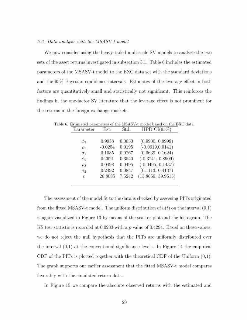
5.2. Data analysis with the MSASV-t model

We now consider using the heavy-tailed multiscale SV models to analyze the two

sets of the asset returns investigated in subsection 5.1. Table 6 includes the estimated

parameters of the MSASV-t model to the EXC data set with the standard deviations

and the 95% Bayesian confidence intervals. Estimates of the leverage effect in both

factors are quantitatively small and statistically not significant. This reinforces the

findings in the one-factor SV literature that the leverage effect is not prominent for

the returns in the foreign exchange markets.

Table 6: Estimated parameters of the MSASV-t model based on the EXC data.


φ1 0.9958 0.0030 (0.9900, 0.9999)ρ1 -0.0254 0.0195 (-0.0619,0.0141)σ1 0.1085 0.0267 (0.0639, 0.1624)φ2 0.2621 0.3540 (-0.3741, 0.8909)ρ2 0.0498 0.0495 (-0.0495, 0.1437)σ2 0.2492 0.0847 (0.1113, 0.4137)v 26.8085 7.5242 (13.8659, 39.9615)

The assessment of the model fit to the data is checked by assessing PITs originated

from the fitted MSASV-t model. The uniform distribution of u(t) on the interval (0,1)

is again visualized in Figure 13 by means of the scatter plot and the histogram. The

KS test statistic is recorded at 0.0283 with a p-value of 0.4294. Based on these values,

we do not reject the null hypothesis that the PITs are uniformly distributed over

the interval (0,1) at the conventional significance levels. In Figure 14 the empirical

CDF of the PITs is plotted together with the theoretical CDF of the Uniform (0,1).

The graph supports our earlier assessment that the fitted MSASV-t model compares

favorably with the simulated return data.

In Figure 15 we compare the absolute observed returns with the estimated and

29

100 200 300 400 500 600 700 800 9000

0.2

0.4

0.6

0.8

1

0 0.1 0.2 0.3 0.4 0.5 0.6 0.7 0.8 0.9 10

0.5

1

1.5

Figure 13: Analysis of the PITs from the MSASV-t model based on EXC data. The top panel showsthe scatter plot of u(t) while the bottom panel shows the histogram of u(t).

0 0.1 0.2 0.3 0.4 0.5 0.6 0.7 0.8 0.9 10

0.1

0.2

0.3

0.4

0.5

0.6

0.7

0.8

0.9

1CDF comparison


Figure 14: Comparison between the CDF of the uniform distribution U(0, 1) and the empirical CDFof the PITs from the MSASV-t model based on the EXC data.

30

forecasted volatilities. The fitted and forecasted volatilities appear to track closely

the absolute values of the observed asset returns. The time series of the estimated

two factors are compared with the absolute observed returns in Figure 16.

100 200 300 400 500 600 700 800 9000

2

4

Time series of observed returns

100 200 300 400 500 600 700 800 9000

2

4


100 200 300 400 500 600 700 800 9000

2

4


Figure 15: Comparison between the absolute returns and the one-step-ahead forecasted volatilitiesunder the MSASV-t model based on the EXC data.

For the AUX return data, the estimated parameters, their confidence intervals

and related standard deviations are presented in Table 7. The leverage effect in

both factors in the MSASV-t model is estimated with the correct expected sign,

and is quantitatively large and statistically highly significant. This suggests that the

leverage effect is a prominent feature of the returns in the equity markets, in keeping

with much of the findings in the one-factor SV literature.

The overall model fit assessment is conducted by the test of the PITs calculated

from the fitted model. The uniform distribution of u(t) on the interval (0,1) is visu-

alized in Figure 17 through the scatter plot and the histogram. The KS test statistic

is calculated at 0.0362 with a p-value of 0.4867. Based on these values, we do not


(0,1) at the conventional significance levels. In Figure 18 the empirical CDF of the

31

100 200 300 400 500 600 700 800 9000


100 200 300 400 500 600 700 800 9000

5


+h2t

)/2

100 200 300 400 500 600 700 800 9000

5


)/2

100 200 300 400 500 600 700 800 9000

5


)/2

Figure 16: Time series of the absolute returns (first panel). Posterior mean of (h1t + h2t)/2 (secondpanel). Posterior mean of slow mean reverting of h1t/2 (third panel) and the posterior mean of fastmean reverting of h2t/2 (fourth panel) based on the MSASV-t model for the EXC data.

Table 7: Estimated parameters of the MSASV-t model based on the AUX data.


φ1 0.9914 0.0034 (0.9845, 0.9976)ρ1 -0.6085 0.0888 (-0.7762,-0.4344)σ1 0.1220 0.0190 (0.0854, 0.1596)φ2 0.3320 0.3615 (-0.3887, 0.8987)ρ2 -0.3162 0.1909 (-0.6933, 0.0468)σ2 0.2376 0.0759 (0.1057, 0.3859)v 24.8652 5.9030 (14.5099, 34.9719)

32

PITs is depicted together with the theoretical CDF of the Uniform (0,1). The graph

reinforces our earlier assessment that the fitted MSASV-t model agrees extremely

well with the asset returns data.

200 400 600 800 1000 1200 14000

0.2

0.4

0.6

0.8

1

0 0.1 0.2 0.3 0.4 0.5 0.6 0.7 0.8 0.9 10

0.5

1

1.5

Figure 17: Analysis of the PITs from the MSASV-t model based on AUX data. The top panel showsthe scatter plot of u(t) while the bottom panel shows the histogram of u(t).

0 0.1 0.2 0.3 0.4 0.5 0.6 0.7 0.8 0.9 10

0.1

0.2

0.3

0.4

0.5

0.6

0.7

0.8

0.9

1CDF comparison


Figure 18: Comparison between the CDF of the uniform distribution U(0, 1) and the empirical CDFof the PITs from the MSASV-t model based on the AUX data.

Figure 19 compares the absolute observed returns with the estimated and one-step-

ahead in-sample and out-of-sample forecasted volatilities. The forecasted volatilities

appear to track very closely the true time series of the absolute returns. The time

series of the estimated two factors are compared with the absolute observed returns

in Figure 20.

33

200 400 600 800 1000 1200 14000

1

2

3Time series of absolute returns

200 400 600 800 1000 1200 14000

1

2

3Estimated return time series from MCMC

200 400 600 800 1000 1200 14000

1

2

3One−step−ahead forecasted volatility time series

Figure 19: Comparison between the absolute returns and the one-step-ahead forecasted volatilitiesunder the MSASV-t model based on the AUX data.

200 400 600 800 1000 1200 14000


200 400 600 800 1000 1200 14000

5


+h2t

)/2

200 400 600 800 1000 1200 14000

5


)/2

200 400 600 800 1000 1200 14000

5


)/2

Figure 20: Time series of the absolute returns (first panel). Posterior mean of (h1t + h2t)/2 (secondpanel). Posterior mean of slow mean reverting of h1t/2 (third panel) and the posterior mean of fastmean reverting of h2t/2 (fourth panel) based on the MSASV-t model for the AUX data.

34

As we did previously in section 5.1, we compare the proposed MSASV-t model

with the heavy-tailed one-factor asymmetric SV (ASV-t) model where the innovation

of asset returns is assumed to have a Student-t distribution and is correlated with

the innovation of the latent factor process. The two data sets are also fitted by the

heavy-tailed one-factor ASV-t model. Table 8 lists the values of D, PD and DIC

calculated based on the fitted MSASV-t and heavy-tailed one-factor ASV-t models.

It is observed that the MSASV-t model fits the EXC data better than the heavy-tailed

one factor ASV-t model, while for the AUX data, the heavy-tailed one-factor ASV-t

model does a better job. The estimated degrees of freedom in the fitted MSASV-t and

the heavy-tailed ASV-t models are greater than 20, so that the variances of the two

Student-t distributions are very close to unity. Furthermore, the DIC values calculated

for the two fitted heavy-tailed models are quite similar in magnitude indicating that

the AUX data can be fitted equally well by the two heavy-tailed factor models.

Table 8: Model selection for the two sets.

Panel A: MSASV-t modelCriterion EXC AUX

D 1762.1 3020.9PD 34.80 43.77DIC 1796.9 3064.7

Panel B: ASV-t modelCriterion EXC AUX

D 1768.2 2994.1PD 38.41 32.47DIC 1806.6 3059.0

6. Conclusion

We have proposed a new variant of multiscale SV models to model the dynamics

of asset returns. The logarithm of conditional volatilities of asset returns is described

35

by latent AR(1) processes with different scales. In order for the proposed model to

accommodate heavy tails in the marginal distribution of asset returns, the innova-

tion of asset returns is assumed to follow a student-t distribution. Suitable MCMC

methods have been developed for parameter estimation of the model. an auxiliary

particle filter is employed to approximate the filtering and prediction distributions

of the latent states of the model when we calculate model likelihood and perform

volatility forecasting. In this paper, we allow for correlation between the innovation

of the mean equation and those of the latent factor processes, which loosely defines

the leverage effect much in keeping with the one-factor SV literature. But we do not

allow for correlation between the innovations of latent AR(1) processes for reason of

computational tractability. This is an issue left for future research.

Appendix A. Multiscale Stochastic Volatility Model

For convenience, we reproduce the continuous-time multiscale SV model discussed

in Molina, Han and Fouque (2010) which motivates the model in (4) - (6) as its

discrete-time approximation.

Let S(t) be the stock price at time t. Let K be the number of volatility factor

driving the one-dimensional S(t), such that the volatility of S(t) is the exponential

sum of K volatilities obeying Ornstein-Uhlenbeck processes:

dS(t) = κS(t)dt+ σ(t)S(t)dW (0)(t)

log(σ2(t)) = F (1)(t) + · · ·+ F (K)(t)

dF (j)(t) = αj + (µj − F (j)(t))dt+ βjdW(j)(t), j = 1, · · · , K (A.1)

where κ is the time-invariant rate of return, αj is the speed of mean reversion of

volatility of the F (j)(t) factor toward its long-run mean level µj, βj is volatility of

36

volatility of the F (j)(t) factor, and W (0)(t) and W (j)(t) for j = 1, · · · , K are possibly

mutually correlated Brownian motions.

Note that 1/αj is a typical time scale of the F (j)(t) factor and they are defined

as well separated, and ordered by assuming that 0 < α1 < α2 for K = 2, so that the

first factor can be interpreted as the longest time scale and the second factor as the

shortest time scale.

Given a constant time step (∆), the Euler-Maruyama discretization scheme is

applied to S(t) and F (j)(t) for j = 1, · · · , K at time point tk = k∆ to yield:

S(tk+1)− S(tk) = κS(tk)∆ + σ(tk)√

∆ε(tk)

log(σ2(tk)) = F1(tk) + · · ·+ FK(tk)

Fj(tk)− Fj(tk−1) = αj + (µj − Fj(tk))∆ + βj√

∆ηj(tk), j = 1, · · · , K (A.2)

where ε(tk) and ηj(tk) for j = 1, · · · , K are possibly mutually correlated sequences of

i.i,d (initially) normal random variables. In the simplest case, the sequence of ε(tk)’s

is initially assumed to be independent of ηj(tk)’s but the ηj(tk)’s can be pairwise

correlated. However, in the equity markets, market participants operate at different

time scales (and based on different information sets), but not independently, and

where the leverage effect is pronounced.

The above discretely approximated model can be rewritten as

1√∆

[S(tk+1)− S(tk)

S(tk

]= σ(tk)ε(tk)

log(σ2(tk)) = F1(tk) + · · ·+ FK(tk)

Fj(tk)− µj = (1− αj)(Fj(tk−1)− µj) + βj√

∆ηj(tk), j = 1, · · · , K (A.3)

37

Next, we define returns in the usual way as

ytk :=1√∆

[S(tk+1)− S(tk)

S(tk− κ∆

]

and write the discrete-time driving vector of volatilities as h(tk)− F(tk − µ) , where

F(tk) = (F1(tk), · · · , FK(tk))′ and µ = (µ1, · · · , µK)′. The autoregressive parameter

is denoted as φj = 1 − αj∆, j = 1, · · · , K. Also we define the standard deviation

parameter as σj,η = βj√

∆, j = 1, · · · , K. Since observations are equally spaced,

with some abuse of notation, we use t instead of tk/∆ for discrete time indices, such

that t ∈ 1, 2, ..., T . This allows us to express a K-dimensional AR(1) process for

log-volatilities in state-space form as

yt = exp((1′ht + 1′µ)/2

)εt, t = 1, · · · , T

ht+1 = Φht + Σ1/2ηt+1, t = 1, · · · , T

h0 ∼ N(0,Ω) (A.4)

where ηt = (η1,t, · · · , ηK,t)′ is the vector of standard random Gaussian variates, 1

is a K-dimensional vector of ones, Φ is a K-dimensional autoregressive (diagonal)

matrix with typical elements φj, and Σ is the covariance matrix, assumed to be

diagonal since the correlation parameter between the factors is not identifiable. The

original version of the model assumes that the Brownian motions driving S(t) and

F (t) are independent and the components of F(t) are driven by independent Brownian

motions. Our discretized model is based on an extension of the original model in which

the components of F (t) are assumed to be correlated to the Browning motion driving

S(t). That is, the original model assumes no correlation between the asset return and

its volatility, our discretized model is based on the extension of the original model

which allows for the so-called leverage effect observed in equity markets. In fact,

38

Black (1976) and Christie (1982) observed that a decrease of the stock price implies

an increase of the associated volatility.

In section 2 of the main text we make precise the parameterization of the discrete-

time multiscale stochastic-volatility model used in both the simulation and estimation

processes, including the initial state and random variable notation.

References

Akaike, H. 1987. Factor Analysis and AIC. Psychometrika 52: 317-332.

Berg, A., R. Meyer, and J. Yu. 2004. Deviance Information Criterion for Comparing

Stochastic Volatility Models. Journal of Business and Economic Statistics 22: 107-

120.

Bauwens, L., Lubrano, M. 1998. Bayesian inference on GARCH models using the

Gibbs sampler. Econometrics Journal 1, C23-C26.

Black, F., 1976. Studies of Stock Price Volatility Changes. Proceedings of the Business

and Economics Section of the American Statistical Association 177-181.

Christie, A., 1982. The Stochastic Behavior of Common Stock Variances: Value,

leverage, and Interest Rate Effects. Journal of Financial Economics 10: 407-432.

Chib, S., F. Nardari, and N. Shephard. 2002. Markov Chain Monte Carlo Methods for

Generalized Stochastic Volatility Models. Journal of Econometrics 108: 281-316.

Chib, S., F. Nardari, and N. Shephard. 2006. Analysis of High Dimensional Multi-

variate Stochastic Volatility Models. Journal of Econometrics 134: 341-371.

Chib, S., Y. Omori, and M. Asai. 2009. Multivariate Stochastic Volatility. Handbook

of Financial Time Series, Springer-Verlag Berlin Heidelberg.

39

Diebold, F. X., T. A. Guther, and A. S. Tay. 1998. Evaluating Density Forecasts with

Applications to Financial Risk Management. International Economic Review 39:

863-883.

Geweke, J. (1993). Bayesian treatment of the independent Student-t linear model.

Journal of Applied Econometrics 8, S19-S40.

Harvey, A. C., E. Ruiz, and N. Shephard. 1994. Multivariate Stochastic Variance

Models. Review of Economic Studies 61: 247-264.

Harvey, A. C., and N. Shephard. 1996. Estimation of an Asymmetric Stochastic

Volatility Model for Asset Returns. Journal of Business &Economic Statistics 14:

429-434.

Jacquier, E., Polson, N. G. and Rossi, P. E. 1994. Bayesian analysis of stochastic

volatility models (with discussion). Journal of Business & Economic Statistics 12,

371-417.

Jacquier, E., N. G. Polson, and P. E. Rossi. 2004. Bayesian Analysis of Stochastic

Volatility Models with Fat-tails and Correlated Errors. Journal of Econometrics

122: 185-212.

Kim, S., N. Shephard, and S. Chib. 1998. Stochastic Volatility: Likelihood Inference

and Comparison with ARCH Models. Review of Economic Studies 65: 361-393.

Lopes H., and Polson N. 2010. Bayesian Inference for Stochastic Volatility Modeling,

in Bocker, K. (Ed.) Rethinking Risk Measurement and Reporting: Uncertainty,

Bayesian Analysis and Expert Judgment, 2010: 515-551.

Meyer, R., and J. Yu. 2000. BUGS for a Bayesian Analysis of Stochastic Volatility

Models. Econometrics Journal 3: 198-215.

40

Molina, G, C. H. Han, and J. P. Fouque. 2010. McMC Estimation of Multiscale

Stochastic Volatility Models. Handbook of Quantitative Finance and Risk Manage-

ment Chapter 71: 1109-1120.

Neal, R. N. 2003. Slice sampling. The Annals of Statistics 31, 705-767.

Pitt, M., and N. Shephard. 1999. Filtering via Simulation: Auxiliary Particle Filters.

Journal of the American Statistical Association 94: 590-599.

Schwarz G. 1978. Estimating the Dimension of a Model. Annals of Statistics 6(2):

461-464.

Shephard, N., and M. K. Pitt. 1997. Likelihood Analysis of non-Gaussian Measure-

ment Time Series. Biometrika 84: 653-667.

Skaug, H., and I. Yu. 2008. Automated Likelihood Based Inference for Stochastic

Volatility Models. Working Paper, Singapore Management University.

Spiegelhalter, D. J., N. G. Best, B. P. Carlin, and A. van der Linde. 2002. Bayesian

Measures of Model Complexity and Fit (with discussion). Journal of the Royal

Statistical Society, Ser. B 64: 583-639.

Taylor, S. J. 1986. Modeling Financial Time Series. Chichester, UK: Wiley.

Yu, J. 2011. Simulation-Based Estimation Methods for Financial Time Series Models.

Handbook of Computational Finance, Chapter 15, Page 427-465.

Yu, J., Yang, Z., Zhang, X. 2006. A class of nonlinear stochastic volatility models

and its implication for pricing currency options. Computational Statistics and Data

Analysis 51, 2218-2231.

Zhang, X., and L. King. 2008. Box-Cox Stochastic Volatility Models with Heavy Tails

and Correlated Errors. Journal of Empirical Finance 15: 549-566.

41

university of waterloo | university of waterloo - …...multiscale stochastic volatility model with...

Documents