university of warwick institutional repository article

University of Warwick institutional repository This paper is made available online in accordance with publisher policies. Please scroll down to view the document itself. Please refer to the repository record for this item and our policy information available from the repository home page for further information. To see the final version of this paper please visit the publisher’s website. Access to the published version may require a subscription.

Author(s: Article Title:

Richard James Lampard Party Political Homogamy in Great Britain

Year of publication: 1997

Link to published version: http://esr.oxfordjournals.org/cgi/content/abstract/13/1/79 Publisher statement: This is a pre-copy-editing, author-produced PDF of an article accepted for publication in European Sociological Review following peer review. The definitive publisher-authenticated version Lampard, R. (1997). Party Political Homogamy in Great Britain. European Sociological Review, 13, pp. 79-99 is available online at:

http://esr.oxfordjournals.org/cgi/content/abstract/13/1/79

1

PARTY POLITICAL HOMOGAMY IN GREAT BRITAIN

[Pre copy-editing version: August 1995]

Richard James Lampard

Department of Sociology, University of Warwick, UNITED KINGDOM.

Richard Lampard is a Lecturer in Sociology at the University of Warwick. Much of his research has been in the area of marriage and divorce, but he also has research interests in social stratification and social statistics (especially the analysis of contingency tables and of event history data). He is currently working on an ESRC-funded project looking at the remarriage process.

Biographical note:

Dr. R.J. Lampard, Mailing address:

Department of Sociology, University of Warwick, Coventry CV4 7AL, UNITED KINGDOM.

2


ABSTRACT This paper focuses on husbands' and wives' party political

identifications in combination. There is a high level of party political

homogamy in Great Britain (i.e. spouses tend to share the same party political

identification). Statistical analyses show that levels of homogamy vary

according to strength of party political identification, parental homogamy, age

and marital status. Levels of party political similarity are also shown to differ

between marriage and other social relationships, and between first marriages

and remarriages. Attitudes towards homogamy are shown to vary with age.

The implications of these findings for theories relating to the origins of

homogamy and to the consequences of heterogamy are considered. Broadly

speaking, the findings indicate that party political homogamy is a consequence

of demographic constraints, utility-maximising choices, and responses to

cultural norms.

3


INTRODUCTION

Research focusing on the joint characteristics of spouses stretches back over

five decades. Early studies demonstrated that there was a tendency towards

homogamy (i.e. like marrying like) for a variety of characteristics. More recent

research has examined trends in educational, religious, class, social status and

ethnic homogamy (Penn & Dawkins, 1983; Ultee & Luijkx, 1990; Mare,

1991; Kalmijn, 1991a; 1991b; 1994; Lampard, 1992; Stier and Shavit, 1994).

Some pieces of recent research have focused on marital status and party

politics (e.g. Kingston & Finkel, 1987; Plutzer & McBurnett, 1991). Other

researchers have examined the effects of spouses' socio-economic

characteristics on their political partisanship and voting behaviour (De Graaf

and Heath, 1992; Hayes and Jones, 1992). However, while Huckfeldt and

Sprague (1991) note that the analysis of political influence between spouses is

worthy of extended attention, little research has been done on party political

homogamy, i.e. the extent to which marriage partners have the same party

political identification and/or vote the same way (though see Brickell et al.,

1988). This may reflect a shortage of data corresponding to samples of couples

as opposed to samples of married individuals.

In addition to its relevance to the discipline of political science, party

political homogamy is also of theoretical interest in the context of theories

relating to the origins and consequences of homogamy and heterogamy.

Heterogamy (i.e. the marriage of dissimilar spouses) has often been viewed as

a source of marital instability, despite a shortage of empirical evidence in

4

support of this hypothesis (Glenn et al, 1974). The hypothesis that party

political heterogamy generates marital conflict would seem as plausible as any

other hypothesis focusing on a specific form of heterogamy.

Turning to the origins of homogamy, a number of different explanations

have been put forward for the tendency of spouses to be similar to each other

across a wide range of different characteristics. These explanations can be

divided into three broad categories: cultural explanations, economic or utility-

maximisation explanations, and explanations focusing on demographic

constraints. All these forms of explanation are evident, whether explicitly or

implicitly, in the recent homogamy-related work of Kalmijn, whose theoretical

discussions involve references to cultural matching, economic competition,

preferences, opportunities and constraints (Kalmijn, 1991a; 1991b; 1994).

Theoretical Explanations of Homogamy

The first type of explanation is one which was implicitly prevalent in the first

few decades of homogamy-related research. People were assumed to adhere to

cultural norms which emphasised the negative and even stigmatic aspects of

dissimilarity between spouses (e.g. Hollingshead, 1950; Kerckhoff, 1963).

Economic explanations of homogamy followed on from the rise to

prominence of rational-choice theory. The most notable proponent of this type

of explanation of homogamy is Gary Becker (Becker, 1991). Essentially this

theoretical perspective focuses on the personal, primarily economic,

advantages gained by marrying a partner with specific characteristics. As such

the first two types of explanation are not entirely distinct from each other,

since gains and losses through adherence to or rejection of cultural norms

5

could be included within the framework of an economic cost-benefit analysis.

In fact the overlap between the two types of explanation corresponds

reasonably well to exchange theory (Blau, 1964), which is rather more

sociologically-orientated than Becker's ideas.

Becker showed that assortative mating for socio-economic

characteristics can be seen as a consequence of competition within the

marriage market for spouses with desirable (i.e. high) levels of economic

resources. The same logic cannot be used to explain party political

homogamy, since it is not simply a by-product of socio-economic homogamy,

and since the costs or benefits of a spouse with a particular party political

identification are primarily non-economic. Party political homogamy can be

expected to play a positive role in reinforcing spouses' values and beliefs,

whereas party political heterogamy can be expected to generate conflict, at the

very least in those cases where the disparity is an extreme one. For this reason

it is probably more appropriate to think in terms of utility maximisation

explanations of party political homogamy rather than in terms of economic

explanations.

The final type of explanation is evident in two sets of published

research. First, choice-based explanations of homogamy have been contrasted

with constraint-based explanations in the debate sometimes referred to as

`homogamy versus propinquity'. Various authors have attempted to ascribe at

least a proportion of observed homogamy to geographical or spatial factors by

asserting that residential and social segregation result in local marriage

markets in which the pools of potential marriage partners are each more

internally homogeneous than the pool of potential marriage partners in the

6

wider population. (Kerckhoff, 1963; Catton and Smircich, 1964; Ramsoy,

1966; Peach, 1974; Morgan, 1981). Second, more overtly theoretical work by

Blau has attempted to assess the impact of the distributions of people among

social positions on their social relations (Blau, 1977: ix). This has led to more

specific pieces of research examining the effects of the social composition of a

population on intermarriage rates between the groups within it (Blau et al.,

1982; Blau et al., 1984). The important aspect of Blau's work is that it

emphasises the role of strictly demographic aspects of social structure in

determining patterns of social association.

The dual aims of this paper are to document party political homogamy

in Great Britain and to link the observed patterns to theoretical ideas relating

to homogamy and heterogamy. The next section therefore uses the various

theoretical explanations of the tendency towards homogamy to generate

hypotheses relevant to the empirical analyses carried out in this paper.

Hypotheses and Predictions relevant to the Empir ical Analyses in this

paper .

This section mirrors the structure of the later section devoted to analyses and

results. The starting point of that section is an examination of the extent of

homogamy of party political identification and of homogamy of voting

intention. This is followed by a multivariate analysis examining the effects of

various relevant factors on the likelihood of homogamy.

One of these factors is strength of party political identification. While

the theoretical explanations of homogamy would predict greater levels of party

political homogamy than would be expected by chance, the theoretical

7

explanations are a little less consistent in terms of what they would predict

about the relationship between strength of party political identification and the

extent of homogamy. The utility-maximisation explanation would predict a

low level of homogamy among those with weak party political identifications

and a high level of homogamy among those with strong party political

identifications, since in terms of conflict avoidance and identity confirmation

homogamy is of greater utility to the former than to the latter. The cultural

explanation would predict a similar, though less marked, relationship, since

people for whom politics are particularly salient may be more likely to

conform to a norm of homogamy. The demographic explanation would predict

a similar relationship if and only if individuals with stronger party political

identifications move in significantly more homogeneous social circles than

individuals with weaker party political identifications.

The multivariate analysis also examines the extent to which the children

of parents who are heterogamous in terms of party political identification

follow in their parents' footsteps. The utility-maximisation explanation of

homogamy would seem to imply that the children of such parents should be

disproportionately homogamous, since any experience of parental conflict due

to heterogamy should predispose the children against heterogamy. Conversely,

the cultural explanation of homogamy would suggest that these children

should be disproportionately heterogamous, since their parents' marriages do

not reinforce the cultural norm. The implications of the demographic

explanation in this context are unclear, though arguably one might expect the

children to move in similar social circles to their parents and hence have a

similar tendency towards homogamy or heterogamy.

8

A third factor considered in the multivariate analysis is age. A

relationship between age and the extent of party political homogamy could

reflect the implications of the various explanations of homogamy in a number

of ways. Increasing homogamy with age could reflect a decline in the strength

of the cultural norm of homogamy, or an attempt by some partners in

heterogamous marriages to conform to this cultural norm by adopting the

party political identification of their spouses. It could also relate to the

dissolution of low utility heterogamous marriages, or to a pragmatic attempt

by some partners within heterogamous couples to reduce conflict by moving

in the political direction of their spouses. A demographic explanation of such a

relationship would need to involve a trend in the internal party political

homogeneity of the social circles into which society is divided, unless the

trend related to the different levels of homogamy induced by the different

demographic constraints of the marriage market and the remarriage market.

A fourth factor considered in the multivariate analysis is `marital status'

(i.e. dating; cohabiting; legally married). A relationship between marital status

and the extent of homogamy could reflect the greater extent to which a

cultural norm of homogamy might apply to legal marriages, or to the greater

reduction in utility attached to conflict and lack of value reinforcement in a

`longer-term' relationship than in a `shorter-term' one. It is not obvious why

the tendency towards homogamy induced by demographic constraints should

vary with marital status; however demographic explanations of homogamy

might be pertinent to any relationship between age at marriage and

homogamy, since the homogeneity of the social circles that one moves in may

vary over one's life-cycle. Marriages at young ages might also be expected to

9

conform less to a cultural norm of homogamy than marriages at older ages;

they might also be marked by a tendency to assess the utility of relationships

less accurately, which would result in a higher level of heterogamy (Becker,

1991).

A separate analysis in the empirical section of this paper considers party

political homogamy in comparison with party political similarity in the context

of other social relationships. If British society is to some extent stratified along

party political lines, whether as a result of individual choices or simply as a

result of the political homogeneity of particular social contexts, one would

expect party political similarities between friends, co-workers, neighbours, etc.

One would also expect some degree of party political homogeneity within

families because of socialization, common economic situations, etc. The

demographic explanation of party political homogamy would predict that

individuals would have levels of party political similarity to their spouses

comparable with their levels of similarity to other people within their social

circles. The cultural and utility-maximisation explanations of homogamy

would both predict that levels of similarity between spouses would be higher

than levels of similarity between neighbours, friends, etc., because the cultural

norm of homogamy would rule out the politically dissimilar members of the

social circles that an individual moves in as potential spouses, and because the

loss of utility attached to conflict with a spouse, and the gain in utility through

consensus with a spouse, would be greater than the corresponding losses and

gains resulting from party political dissimilarity and similarity within other

forms of relationship.

The last set of empirical analyses in this paper focus on the possible

10

linkage between homogamy and marital success. One issue of interest in this

context is the extent to which the population perceives agreement on politics

as being important for a successful marriage. The cultural explanation of

homogamy would, of course, predict that a high proportion of the population

would see agreement on politics as important in this context. It is less clear

whether the utility-maximisation explanation would predict this, as the

decision to carry on or to end a relationship which might become a marriage-

type relationship may not consciously involve a recognition of the role of

party politics in generating conflict or strengthening consensus. The

demographic explanation would not in itself predict that agreement on politics

would be perceived to be important to a successful marriage.

The final analysis in this paper focuses on differences in the extent of

homogamy between first marriages and remarriages. All three explanations of

homogamy are potentially relevant in this context. The cultural explanation

can be argued to predict greater heterogamy in remarriages, since the divorced

have failed to adhere to another marriage-related norm, i.e. life-long marriage.

The utility-maximisation explanation is ambiguous in its predictions, since on

one hand people marrying for a second time may be more careful in their

assessment of the utility of the relationships, but on the other hand these

people may be disproportionately poor at correctly assessing the utility of

relationships, and hence may be inclined to enter into fragile, heterogamous

marriages. The demographic explanation would predict differential levels of

homogamy in relation to the relative levels of party political homogeneity of

social circles within the marriage and remarriage markets; since the remarriage

market is likely to be more fragmented and to involve a smaller proportion of

11

the population, remarriages might be expected to be more heterogamous than

first marriages.

To conclude this section, it is important to note that the degree of

overlap between the predictions based on the various explanations of

homogamy means that assessing their relative merits is likely to be difficult.

However, by carrying out a range of empirical analyses it may be possible to

generate evidence which suggests that one or more of the explanations are

correct and are of particular importance.

DATA SOURCES

This paper uses data from a number of sources. The 1987 British General

Election Survey (BES) surveyed a stratified multi-stage random sample of

British adults aged 18 or over living in private households. Fieldwork was

carried out from June to September 1987, and a 70% response rate gave rise to

an achieved sample size of 3,826 (see Heath et al., 1991: 230-234). The 1992

British General Election Survey (see Heath et al., 1993) is also used in this

paper to check the validity of the data used from the 1987 survey.

The 1986 British Social Attitudes Survey (BSAS) also surveyed a

stratified multi-stage random sample of British adults aged 18 or over living in

private households. Fieldwork was carried out in April to May 1986, and a

70% response rate led to an achieved sample size of 3,100 (see Jowell et al.,

1987: 187-194).

The 1986 ESRC Social Change and Economic Life Initiative (SCELI)

work attitudes\histories survey surveyed random samples of adults aged

between 20 and 60 in the non-institutional populations of six urban local

12

labour markets in Britain (Aberdeen, Coventry, Kirkcaldy, Northampton,

Rochdale and Swindon). Fieldwork was carried out in June to November 1986

and a 76% response rate led to an achieved sample size of 6,111. The SCELI

Household and Community Survey was a follow-up survey of a subset of

these respondents. In this second survey, where applicable, a range of

questions was asked of the respondent's partner as well as of the original

respondent. Fieldwork was carried out between March and July 1987, and the

response rate of this follow-up survey was 76%, leading to a sample size of

1,816, of whom 1,218 were living in partnerships (see Gallie, Marsh and

Vogler, 1994: 337-346).

All three of the above surveys used the electoral register as their

sampling frame, and in each case the survey data have been deposited at, and

are available from, the ESRC Data Archive at the University of Essex.

The BES collected data about the party political identifications both of

its respondents and of some of their partners. However, there are two major

limitations to these data. First, the data relating to respondents' partners were

collected by a series of questions which were geared towards identifying the

party political identifications of the two people with whom each respondent

discussed politics most often during the 1987 General Election campaign.

Consequently, if a respondent's partner was not one of these two people, no

data were collected about the partner's party political identification. Second,

the accuracy of the data collected depends on whether the respondent was

aware of and reported correctly their partner's party political identification.

Thus analyses of the BES data need to be supported by evidence from

other sources which indicate that the data are adequately representative and of

13

adequate validity, e.g. data from the SCELI Household and Community

Survey, which collected data on the voting intentions of a sample of

respondents and their partners in separate self-completion booklets, with no

collaboration being allowed between partners.

The SCELI data are themselves limited, since, while the BES was a

nationally representative survey, SCELI focused on six specific study areas.

However, a comparison of the data from the two sources goes some way

towards establishing whether the BES data are adequately representative and

of adequate validity.

Further details of the key questions from these surveys are given in

footnotes to the tables. In addition to data on party political identifications and

voting intentions from the BES and SCELI surveys, marriage-related

attitudinal data from the 1986 BSAS are also used in this paper.

It is worth noting that the data sources used in this paper are not ideal

for the examination of party political homogamy for a number of reasons.

First, only limited data are available relating to respondents' partners. As a

consequence it is not possible to look at the relationship between party

political homogamy and various other forms of homogamy. In addition, in

some of the analyses in this paper where an independent variable relates to the

respondent it would be useful to have a measure of the same variable for the

respondent's partner (e.g. when looking at the effect of strength of party

political identification on the probability of party political homogamy).

Second, the BES data do not allow one to distinguish between first marriages

and remarriages. The SCELI data allow one to do this, but do not include data

on the previous spouses of remarried respondents. Finally, and most

14

importantly, the data sources are cross-sectional surveys which collected

limited retrospective data and as such are limited in what they can show about

age and cohort effects. There is no way of telling whether a couple who are

currently homogamous for party political identification were homogamous in

this respect at the time of their marriage. This issue will be returned to later in

this paper.

METHODS, ANALYSES AND RESULTS

This section presents empirical analyses relating to party political homogamy

in Great Britain. First, the extent of such homogamy is documented. A

multivariate analysis looking at the effects of various pertinent factors on the

likelihood of heterogamy\homogamy is then presented. This is followed by a

comparison between party political homogamy and party political similarity

within other social relationships. Finally, analyses relevant to the possible

relationship between party political homogamy and marital success are

presented.

In addition to the use of odds ratios as measures of association, the

analyses in this paper involve the use of logistic regressions and hierarchical

log-linear models (Gilbert, 1993). The log-linear models were fitted using

GLIM (see Francis, Green and Payne, 1993), and the logistic regressions were

carried out using SPSS for Windows (Norusis, 1993).

In order to keep this paper reasonably accessible, the findings are to a

large extent presented in the form of cross-tabulations and percentages rather

than parameter estimates. However, since some of the factors affecting the

likelihood of party political homogamy are correlated, a multivariate analysis

15

(specifically in this case a logistic regression) is needed to check that each

factor still has an effect when the other factors are controlled for. A

multivariate analysis also allows any effects of social class and education to be

identified and accounted for; note that some evidence exists that graduate

couples may be unusually homogamous (Lampard, 1992).

An examination of party political homogamy might have been expected

to have utilised even more elaborate multivariate analyses than those used in

this paper. Recent work on assortative mating has shown how it can be useful

to consider the overlap between different forms of homogamy (Kalmijn,

1991a; 1991b; 1994). However, the data sources used in this paper only allow

the relationship between party political homogamy and occupational class

homogamy to be examined.

More complicated multivariate models would have also been useful if

the data sources available had permitted a sophisticated analysis of the effects

of marriage duration, marriage cohort and period on the level of party political

homogamy. However, the data sources used in this paper did not permit such

an analysis.

16

The Extent of Par ty Political Homogamy

2,606 of the BES respondents were married or living as married. Of these,

1,677 (64%) reported that their partner was one of the two people with whom

they discussed politics the most during the 1987 general election campaign. Of

the other 929 respondents, 461 (18% of the total sample) reported not having

discussed politics with anybody during the election campaign and the

remaining 468 (18% of the total sample) reported having discussed politics

with somebody during the election campaign, but reported that their partner

was not one of the two people with whom they discussed politics the most.

Overall, of the 2,145 respondents who reported discussing politics with

someone

In addition to the married or cohabiting respondents, 109 other

respondents reported that their partner was one of the two people with whom

they discussed politics the most during the election campaign. This included a

small number of people whose marriages had since ended, but mainly

consisted of respondents who were part of couple relationships but were not

married to or living with their partners. Overall, data were collected by the

BES on the party political identifications of 1,786 couples.

during the election campaign, 1,677 (78%) reported that their partner

was one of the two people with whom they discussed politics the most.

As will be shown later in this paper, the marital status of couples is

related to the level of homogamy observed. However, restricting attention to

legally married couples, or to couples who were living together, has a minimal

effect on the results of the other analyses in this paper, and the analyses

involving the BES data are therefore based on all the available couples.

Contemporary party politics in Britain has been dominated by the (right-

17

wing) Conservative party and the (left-wing) Labour party, with a third party,

or alliance of parties, occupying the political middle ground. In this paper the

`Alliance' between the Liberal and Social Democratic parties is treated as a

single party.

In 1,591 (89%) of the BES couples both partners identified with one of

the three `main' British political parties, though not necessarily the same party.

In 47 (3%) of the couples one partner identified with one of the three `main'

parties and the other identified with another party. In 11 (1%) of the couples

both partners identified with the same, `minor' party. In the remaining 137

(8%) of the couples, one or both partners did not identify with any party, or

refused to answer the relevant question.

TABLE 1 ABOUT HERE

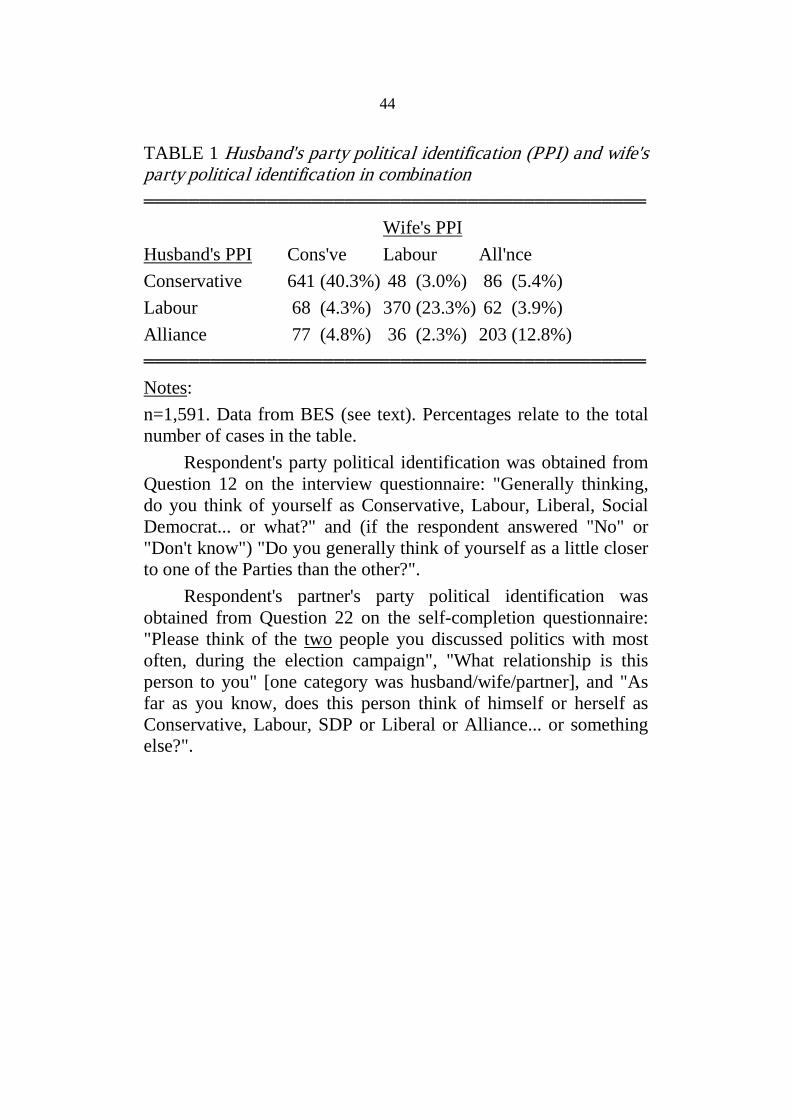
Table 1 shows partners' party political identifications in combination for the

1,591 couples where both partners identified with one of the three `main'

parties. In over three-quarters of the couples the partners both identified with

the same party, and in only one in fourteen couples is there a

Labour/Conservative disparity. (If there had been no relationship between

partners' party political identifications these figures would have been just over

a third and one in five respectively).

Odds ratios can be used to summarise the strength of the relationship

between partners' party political identifications. Restricting attention to

couples involving Conservative identifiers and Alliance identifiers, the odds

ratio is (641x203)/(86x77) = 19.7. Restricting attention to couples involving

Labour identifiers and Alliance identifiers, the odds ratio is (370x203)/(62x36)

= 33.7. Finally, restricting attention to couples involving Conservative

18

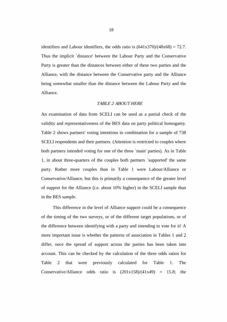
identifiers and Labour identifiers, the odds ratio is (641x370)/(48x68) = 72.7.

Thus the implicit `distance' between the Labour Party and the Conservative

Party is greater than the distances between either of these two parties and the

Alliance, with the distance between the Conservative party and the Alliance

being somewhat smaller than the distance between the Labour Party and the

Alliance.

TABLE 2 ABOUT HERE

An examination of data from SCELI can be used as a partial check of the

validity and representativeness of the BES data on party political homogamy.

Table 2 shows partners' voting intentions in combination for a sample of 738

SCELI respondents and their partners. (Attention is restricted to couples where

both partners intended voting for one of the three `main' parties). As in Table

1, in about three-quarters of the couples both partners `supported' the same

party. Rather more couples than in Table 1 were Labour/Alliance or

Conservative/Alliance, but this is primarily a consequence of the greater level

of support for the Alliance (i.e. about 10% higher) in the SCELI sample than

in the BES sample.

This difference in the level of Alliance support could be a consequence

of the timing of the two surveys, or of the different target populations, or of

the difference between identifying with a party and intending to vote for it! A

more important issue is whether the patterns of association in Tables 1 and 2

differ, once the spread of support across the parties has been taken into

account. This can be checked by the calculation of the three odds ratios for

Table 2 that were previously calculated for Table 1. The

Conservative/Alliance odds ratio is (201x158)/(41x49) = 15.8; the

19

Labour/Alliance odds ratio is (193x158)/(35x30) = 29.0; and the

Labour/Conservative odds ratio is (201x193)/(18x13) = 165.8. Hence the first

two SCELI odds ratios are very similar to those from the BES sample,

whereas the third SCELI odds ratio is considerably larger than that from the

BES sample. This reflects the small number of Labour/Conservative couples

in the SCELI sample (4% of all couples, as opposed to 7% of all couples in the

BES sample).

Tables 1 and 2 were combined to give a three-way table of husband's

party by wife's party by survey. Log-linear models fitted to this table showed

that both the distribution of support across the three parties and the frequency

of Labour/Conservative and Conservative/Labour couples (given the

distribution of support across the parties) varied significantly between the BES

and SCELI samples (p<.001 and p<.05 respectively).

Why should there have been significantly fewer Labour/Conservative

disparities in the SCELI sample? One possibility is that partners' voting

intentions are more similar than their party political identifications as a

consequence of tactical voting. Another is that it is a reflection of peculiarities

of the SCELI study areas, though an examination of the part of the BES

sample corresponding geographically to the SCELI study areas indicated that

if anything the level of heterogamy should have been higher in the SCELI

sample than in the BES sample. Finally, the greater level of support for the

Alliance in the SCELI sample may indicate that some couples who would

have appeared as Labour/Conservative or Conservative/Labour in the BES

sample appeared in the SCELI sample as Labour/Alliance or

Alliance/Conservative. (This is consistent with the slightly lower odds ratios

20

for these two disparities in the SCELI sample as compared to the BES

sample).

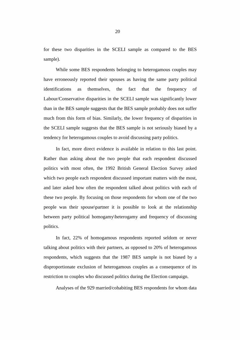
While some BES respondents belonging to heterogamous couples may

have erroneously reported their spouses as having the same party political

identifications as themselves, the fact that the frequency of

Labour/Conservative disparities in the SCELI sample was significantly lower

than in the BES sample suggests that the BES sample probably does not suffer

much from this form of bias. Similarly, the lower frequency of disparities in

the SCELI sample suggests that the BES sample is not seriously biased by a

tendency for heterogamous couples to avoid discussing party politics.

In fact, more direct evidence is available in relation to this last point.

Rather than asking about the two people that each respondent discussed

politics with most often, the 1992 British General Election Survey asked

which two people each respondent discussed important matters with the most,

and later asked how often the respondent talked about politics with each of

these two people. By focusing on those respondents for whom one of the two

people was their spouse\partner it is possible to look at the relationship

between party political homogamy\heterogamy and frequency of discussing

politics.

In fact, 22% of homogamous respondents reported seldom or never

talking about politics with their partners, as opposed to 20% of heterogamous

respondents, which suggests that the 1987 BES sample is not biased by a

disproportionate exclusion of heterogamous couples as a consequence of its

restriction to couples who discussed politics during the Election campaign.

Analyses of the 929 married/cohabiting BES respondents for whom data

21

on spouse's party political identification were not collected showed that the

sample of 1,677 BES respondents for whom these data were collected under-

represented Labour identifiers, those who did not identify with a party, and

those whose party political identifications were not very strong. The next

section shows that respondents in the last category are disproportionately

likely to be heterogamous, hence the sample of 1,677 couples probably

slightly under-represents heterogamous couples. However, an examination of

the magnitude of the relationship between strength of party political

identification and party political homogamy, and of the level of under-

representation of respondents whose party political identifications were not

very strong, indicates that the likely shortfall only constitutes 1% to 2% of

heterogamous couples, i.e. about half-a-dozen cases.

A Multivar iate Analysis of Par ty Political Homogamy

The next few sections discuss the results of logistic regressions with party

political homogamy\heterogamy as the binary dependent variable (heterogamy

= 1; homogamy = 0) and various relevant factors as independent variables.

Table 3 shows the results for all 1,591 respondents in Table 1; Table 4 shows

the results when attention was restricted to respondents who were Labour or

Conservative identifiers and who had Labour or Conservative partners. Data

for quite large numbers of respondents were missing for one or more of the

independent variables, thus in order to avoid a markedly reduced sample size

categories such as `not given' or `unknown' were used for some of the

independent variables.

It can be seen from Tables 3 and 4 that the effects of the social class and

22

education variables are not statistically significant. Social class was based on

respondent's own occupation and was operationalized using a collapsed

version of the Goldthorpe class schema (Heath et al., 1991: 66), the classes

used being a `salariat', routine non-manual workers, the `petty bourgeoisie',

foremen and technicians, and a `working class'. Class heterogamy

(operationalized as one partner in the salariat and one in the working class)

can be seen from Tables 3 and 4 to have a statistically insignificant effect. The

education variable was based on highest qualification.

TABLES 3 AND 4 ABOUT HERE

Homogamy and Strength of Par ty Political Identification

It can be seen from Table 3 that the strength of a respondent's party political

identification has a statistically significant effect on the likelihood of

homogamy. The tendency towards heterogamy increases markedly as the

strength of the respondent's party political identification decreases.

The relevant parameter estimates in Table 3 are very similar to those

obtained in a bivariate analysis of the relationship between party political

homogamy and strength of respondent's party political identification. A more

detailed discussion of this relationship therefore follows.

Table 5 shows the relationship between strength of respondent's party

political identification and partners' party political identifications in

combination

TABLE 5 ABOUT HERE

The proportion of couples who are heterogamous is over three times as

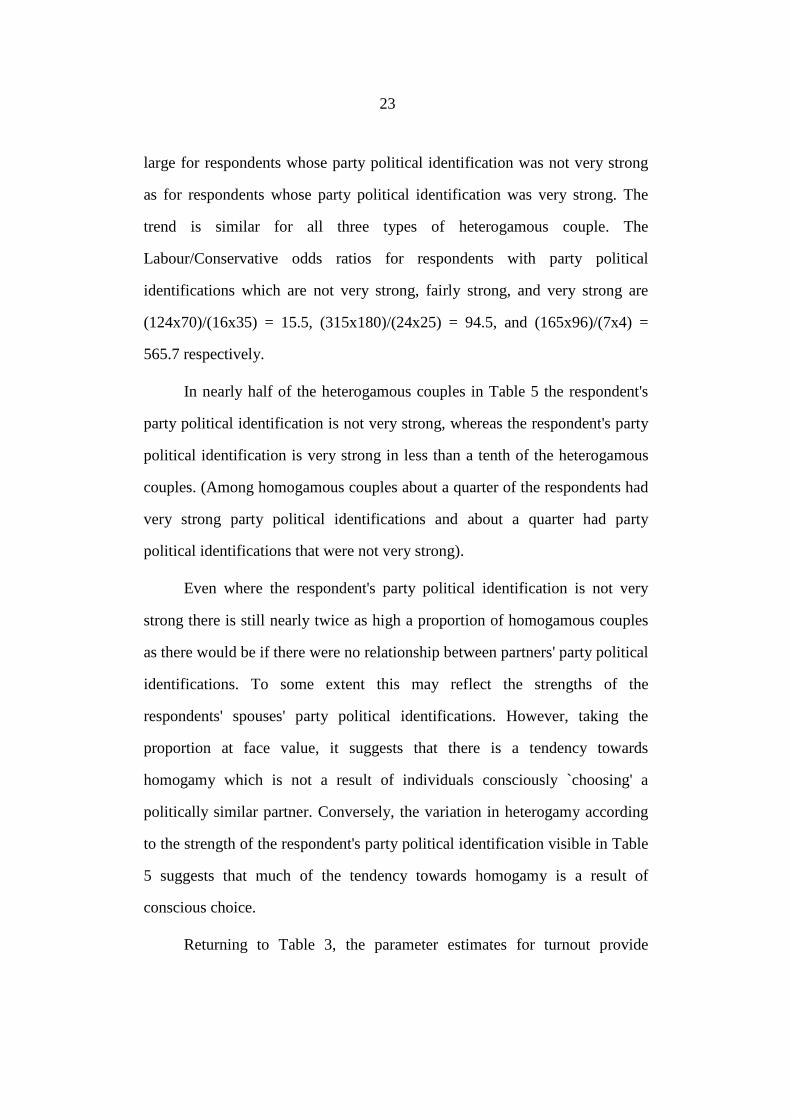
23

large for respondents whose party political identification was not very strong

as for respondents whose party political identification was very strong. The

trend is similar for all three types of heterogamous couple. The

Labour/Conservative odds ratios for respondents with party political

identifications which are not very strong, fairly strong, and very strong are

(124x70)/(16x35) = 15.5, (315x180)/(24x25) = 94.5, and (165x96)/(7x4) =

565.7 respectively.

In nearly half of the heterogamous couples in Table 5 the respondent's

party political identification is not very strong, whereas the respondent's party

political identification is very strong in less than a tenth of the heterogamous

couples. (Among homogamous couples about a quarter of the respondents had

very strong party political identifications and about a quarter had party

political identifications that were not very strong).

Even where the respondent's party political identification is not very

strong there is still nearly twice as high a proportion of homogamous couples

as there would be if there were no relationship between partners' party political

identifications. To some extent this may reflect the strengths of the

respondents' spouses' party political identifications. However, taking the

proportion at face value, it suggests that there is a tendency towards

homogamy which is not a result of individuals consciously `choosing' a

politically similar partner. Conversely, the variation in heterogamy according

to the strength of the respondent's party political identification visible in Table

5 suggests that much of the tendency towards homogamy is a result of

conscious choice.

Returning to Table 3, the parameter estimates for turnout provide

24

statistically significant evidence that heterogamy is disproportionately

frequent among people who do not vote. (The variable relates to actual rather

than stated voting behaviour; see Swaddle and Heath, 1989). In the BES

sample 34% of married non-voters were heterogamous, as opposed to 23% of

married voters (Lampard, 1992). Once again, this is consistent with the

hypothesis that party political homogamy/heterogamy is related to the degree

of salience of party politics to the respondent.

In the vast majority of heterogamous couples the respondent does not

identify very strongly with a party, which suggests that the heterogamy may

not be a problem for the couple. However, conflict is more likely where one

partner objects to the party that the other partner identifies with, hence it is not

so much the strength of the respondent's party political identification which is

of relevance as their attitude towards the party their partner identifies with.

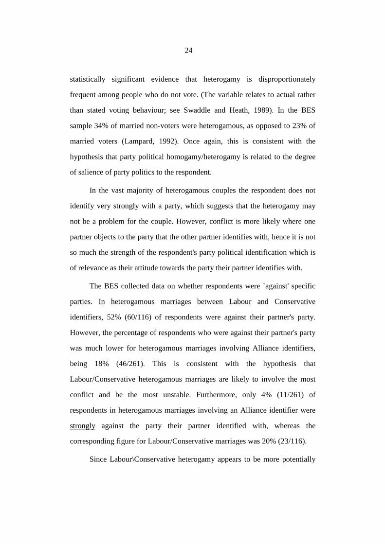
The BES collected data on whether respondents were `against' specific

parties. In heterogamous marriages between Labour and Conservative

identifiers, 52% (60/116) of respondents were against their partner's party.

However, the percentage of respondents who were against their partner's party

was much lower for heterogamous marriages involving Alliance identifiers,

being 18% (46/261). This is consistent with the hypothesis that

Labour/Conservative heterogamous marriages are likely to involve the most

conflict and be the most unstable. Furthermore, only 4% (11/261) of

respondents in heterogamous marriages involving an Alliance identifier were

strongly

Since Labour\Conservative heterogamy appears to be more potentially

against the party their partner identified with, whereas the

corresponding figure for Labour/Conservative marriages was 20% (23/116).

25

problematic than other forms of party political heterogamy, the analyses in the

rest of this paper focus where possible on Labour\Conservative heterogamy as

well as considering party political heterogamy more broadly.

Overall, the respondent was against the party that their partner identified

with in less than one in three of the heterogamous couples in Table 1, and was

only strongly against their partner's party in about one in eleven of the

heterogamous couples.

Hence, if one assumes that party political differences between spouses

are only likely to be problematic in couples where one or both partners is

against the other's party, party political differences are likely to cause

problems in no more than about one in three heterogamous couples, though

this figure is likely to be a slight underestimate, as it does not take account of

couples where the respondent is not against their partner's party, but where the

respondent's partner is against the respondent's party).

The Intergenerational Transmission of Heterogamy

The BES collected data from its respondents on the voting behaviour of their

parents when the respondents were growing up. This allows one to test the

hypothesis that the children of heterogamous parents are more heterogamous

than the children of homogamous parents.

Of the 1,591 respondents in the sub-sample of the BES on which Table

1 was based, 1,217 reported both their parents as having usually voted for one

of the three main parties. The overall percentage of homogamous sets of

parents is 88.3% (1,075/1,217), as compared to 76.3% of the couples in Table

1. This may indicate that some respondents were misrepresenting the voting

26

behaviour of their parents. However, the odds ratio corresponding to

Labour/Conservative homogamy/heterogamy among the parents is

(393x610)/(31x58) = 133.3, which is similar to the corresponding odds ratios

in Tables 1 and 2. The difference between the parents and the couples in

Tables 1 and 2 probably reflects the fact that the Alliance in 1987 was a much

more heterogeneous entity than its predecessor the Liberal party had been in

preceding decades.

32% (46/142) of those BES respondents who reported their parents as

having been heterogamous were heterogamous, compared with 23%

(246/1,075) of respondents with homogamous parents. However, the relevant

parameter estimate in Table 3 is consistent with a percentage difference of this

magnitude and demonstrates that parental heterogamy still significantly

increases the likelihood of heterogamy net of the other independent variables

in the logistic regression. (Note that the corresponding parameter estimate in

Table 4, though not quite statistically significant, is marginally greater in

magnitude). The inclusion of these other variables in the multivariate analysis

rules out some of the most obvious explanations of the intergenerational

transmission of party political homogamy.

Heterogamous parents might be expected to be less strong than average

in their political identifications, and to have an `aggregate' political

identification which is towards the centre of a `Left'/`Right' political

dimension. Two reasonable assumptions about the children of heterogamous

parents follow on from this. First, it seems reasonable to assume that a child of

a heterogamous couple is likely to be a less strong supporter of the party they

identify with than a child of a homogamous couple. The results from the

27

earlier section on homogamy/heterogamy and strength of party political

identification would then suggest that the first child was more likely to be in a

heterogamous marriage. The second reasonable assumption is that a child of a

heterogamous couple is more likely to be an Alliance identifier than a child of

a homogamous couple, and Alliance identifiers are more likely to be in

heterogamous marriages, hence the first child is more likely to be in a

heterogamous marriage. Thus there are two fairly straightforward but rather

uninteresting ways of explaining the intergenerational transmission of

heterogamy.

However, the inclusion of party political identification and strength of

party political identification in the logistic regression demonstrates that the

intergenerational transmission of heterogamy cannot be explained in these

ways.

The statistically significant parameter estimate from the logistic

regression is consistent, however, with the hypothesis is that the children of

party politically heterogamous parents are simply more likely to see party

political heterogamy as acceptable, possibly because they do not see party

politics as of salience in the marital context even if they see it as salient in

other contexts.

The above findings are relevant to more general considerations of the

intergenerational transmission of political attitudes, as they provide some

support for the idea that such attitudes are in part culturally determined rather

than simply reflecting rational economic choices (Butler and Stokes, 1974;

Himmelweit et al., 1981).

28

Homogamy, Age and Mar ital Status

It was noted in the last section that it is possible that respondents' parents were

more homogamous than the respondents were. If a trend towards less

homogamy exists, then one would expect there to be a relationship between

party political homogamy and respondent's age. There is the standard problem

of distinguishing between age and cohort effects, which will be discussed in

more detail a little later. Note that respondent's age is wife's age in some cases

and husband's age in others; though this is not ideal the similarity of spouses'

ages on average means that it is not a serious problem.

The parameter estimate corresponding to respondent's age in Table 3

shows that respondent's age does not have a statistically significant effect on

the overall likelihood of heterogamy, but the corresponding parameter

estimate in Table 4 shows that respondent's age just has a significant effect on

the likelihood of Labour\Conservative heterogamy. This sole age-related

effect corresponds to a dichotomy contrasting respondents aged under 35 years

with those aged 35 or more years.

52 out of 442 (12%) of the respondents aged under 35 in Table 4 are

Labour/Conservative heterogamous, as compared to 64 out of 1,149 (6%) of

the respondents aged 35 or over. Note that some of this percentage difference

is spurious since it is induced by correlations between respondent's age and

respondent's strength of party political identification and between respondent's

age and respondent's marital status. The corresponding figures for other forms

of heterogamy are 78 out of 442 (18%) and 183 out of 1,149 (16%).

The statistically significant relationship between respondent's age and

Labour\Conservative heterogamy evident from the parameter estimate in

29

Table 4 could be a reflection of three distinct time-related processes, which are

difficult to distinguish between given the cross-sectional nature of the data.

First, the relationship between age and Labour/Conservative heterogamy may

reflect a trend across marriage cohorts towards greater heterogamy at the time

of marriage. Second, it may reflect a tendency for couples within a marriage

cohort to become less heterogamous with increasing marriage duration, i.e. as

their marriages `age'. This decrease in heterogamy with increasing marriage

duration has often been hypothesised to occur in the context of spouses'

religions, though Kalmijn found no evidence in his research that this was the

case (Kalmijn, 1991b). Finally, the excess of Labour/Conservative marriages

at younger ages may be due to differential attrition within marriage cohorts,

i.e. politically heterogamous marriages may be more likely to end in divorce.

Overall, the observed relationship is consistent with a relatively recent

increase in Labour\Conservative heterogamy at marriage, or a relatively quick

convergence of the political identifications of some heterogamous couples as

their marriages progress, or the relatively rapid dissolution of the marriages of

some heterogamous couples (or a combination of the three possibilities). Note

that the latter two possibilities both imply that Labour\Conservative marriages

are `problematic'; arguably the first possibility requires an unsatisfactorily

abrupt change in marriage patterns.

One plausible hypothesis relating to the final possibility is that the

excess of heterogamous marriages among respondents under 35 is due to

`hasty' marriages at an early age which will eventually end in divorce (cf

Kiernan, 1986). However, if anything, marriages at an early age seem to be

associated with increased homogamy, since 16% (18/110) of the couples in the

30

SCELI sample where the respondent had married as a teenager were

heterogamous, as opposed to 26% (134/515) of the couples where the

respondent had married in their twenties or later (p<.05).

Marriages at an early age may be unusually homogamous because the

`social circles' that people move in at a young age are more homogeneous with

respect to party politics than those they encounter later in their adult lives.

Mare has suggested a similar relationship in the context of educational

homogamy (Mare, 1991: 16). A later section considers the relationship

between homogamy and social context in more detail.

As noted earlier in this section, the crude relationship between age and

homogamy/heterogamy partly reflects a relationship between marital status

and homogamy/heterogamy. Of the 1,591 couples in Table 1, 59 were

cohabiting and a further 69 were neither legally married nor cohabiting. (In

addition to this, 18 respondents who discussed politics with their partner

during the election campaign were widowed, divorced or separated at the time

they were interviewed).

The relevant parameter estimates in Table 3 show that the general level

of heterogamy is significantly higher among unmarried/non-cohabiting

couples than among cohabiting couples and legally married couples. The

parameter estimate corresponding to unmarried/non-cohabiting couples in

Table 4 is not quite statistically significant but is of a similar magnitude to the

corresponding, statistically significant, parameter estimate in Table 3.

The higher level of heterogamy among couples who are not legally

married and who do not live together is consistent with the hypothesis that the

importance of shared political views becomes greater as the level of

31

commitment in a relationship increases. Thus it may be that people are more

willing to `date' people who do not share their political views than they are to

marry/live with them.

Homogamy and Social Context

It is not just marriage partners who are similar in party political terms. Is the

high level of party political homogamy simply a reflection of the party

political homogeneity of the `social circles' in which people live? An analysis

of BES data can go some way towards answering this question. The data on

party political homogamy/heterogamy came from a question looking at the

party political identifications of the two people with whom respondents

discussed politics the most during the election campaign; this question can

also provide evidence of respondents' party political similarity to members of

their families, co-workers, neighbours and friends.

TABLE 6 ABOUT HERE

Table 6 shows the relationship between respondents' party political

identifications and the party political identifications of individuals belonging

to various categories of relatives/friends/acquaintances. (As in the previous

analyses attention is restricted to cases where both individuals identified with

one of the `main' three parties). Each of the sub-tables only corresponds to a

sub-sample of the overall BES sample. There is no guarantee that the relevant

sub-sample is at all representative of the broader sample, or that the sub-tables

are at all representative of the respondents' relatives/friends/acquaintances in

general. Respondents may have been disproportionately likely (or

disproportionately unlikely) to have discussed politics the most during the

32

Election Campaign with people who shared their party political views. Thus

the findings that follow are based on the assumption that the data in Table 6

are not fatally biased.

The level of party political homogamy in Table 1 (76%) is much the

same as the level of party political similarity visible in Table 6 between

respondents and other members of their families living in the same household

(73%), though the percentage of Labour/Conservative disparities is rather

higher in the first sub-table of Table 6 than it was in Table 1 (11% as

compared with 7%). However, fewer respondents (63%) were similar to

members of their families who were not

The level of similarity of respondents to their neighbours (65%) was

much the same as the level of similarity of respondents to members of their

families who were not living in their households. However, the corresponding

figure for co-workers was much lower than this (49%). The level of similarity

of respondents to friends who were not relatives or neighbours or co-workers

(57%) was also quite low relative to the level of party political homogamy in

Table 1.

living in their households.

The high level of similarity of respondents to other family members

living in the same household probably reflects the `closeness' of the

relationships involved, e.g. parent/child, respondent/sibling. The levels of

similarity in the other four sub-tables of Table 6 are probably more

representative of the level of similarity of respondents to the generality of

individuals in the respondents' `social circles'.

Focusing on the Labour and Conservative identifiers in each sub-table,

the odds ratios corresponding to the neighbours, co-workers and other friends

33

sub-tables are (76x45)/(10x22) = 15.5, (147x124)/(77x58) = 4.1, and

(166x125)/(65x35) = 9.1 respectively, as compared to an odds ratio of 72.7 in

Table 1. Thus some of the tendency towards party political homogamy is not

explained by the general level of party political similarity of respondents to the

people in the `social circles' that they move in. An important part of the

tendency to party political homogamy appears to be a tendency for individuals

to choose

Conversely, the levels of similarity obtained from the sub-tables of

Table 6 suggest that there are structural effects which to an extent lead to party

political homogamy. Of course, individuals exercise a certain amount of

control over who their neighbours, co-workers and other friends are but

decisions leading to individuals moving in particular `social circles' are

probably largely based on factors other than the individual's perception of the

party political views of the people within those social circles, and the party

political homogeneity of many `social circles' is not something over which

individuals can exert much control.

a partner whose party political views match their own. The data in

Table 6 suggest that it is implausible that the observed level of party political

homogamy is entirely a consequence of structural constraints.

Note that the above discussion hinges on the assumption that the data

analysed are adequately representative of the `social circles' within which the

respondents move.

The above findings are consistent with the view of Huckfeldt and

Sprague that the relationship between individual political attitudes and the

prevalent political attitudes in a locality reflect both individual choices and

structural constraints (Huckfeldt and Sprague, 1991; Huckfeldt, Plutzer and

34

Sprague, 1993).

Homogamy and Mar ital Success

While heterogamy is often thought to reduce marital quality and/or increase

marital instability, there is very little evidence to support this hypothesis,

except in the case of age heterogamy (Lampard, 1992), and possibly

educational heterogamy (Tzeng, 1992). However, BSAS data suggest that

many people see homogamy as important to the success of a marriage.

Respondents were provided with a list of factors which might affect the

success of a marriage and were asked the question "How important is each one

to a successful marriage?". Respondents could rate the factors as "Very

Important", "Fairly Important", "Not Very Important" and "Not At All

Important". Four of the listed factors were homogamy-related, i.e. "Tastes and

interests in common", "Same social background", "Shared religious beliefs",

and "Agreement on politics".

"Agreement on politics" was rated as very or fairly important by 15%

(239/1,552) of respondents. However, the corresponding figures for "Tastes

and interests in common", "Same social background", and "Shared religious

beliefs" were 79%, 48% and 37% respectively. Thus, though party political

homogamy is even more common in Britain than homogamy of social origin,

it is not seen as of the same degree of importance in the context of marital

success.

The above findings may reflect a public perception of politics as of little

relevance to everyday life and social interactions. Thus while the party

political homogamy evident in Table 1 reflects the underlying socio-political

35

values and beliefs of BES respondents and their partners, BSAS respondents

may not have interpreted "agreement on politics" as meaning "agreement on

attitudes towards important socio-political issues". Additionally, the `dire

consequences' of religious intermarriage, marrying `cross-class', and marrying

a spouse with different tastes and interests are probably more entrenched in

British minds than the negative consequences of political differences between

spouses are (possibly as a consequence of the infrequency of such political

differences).

54% (126/235) of BSAS respondents who saw "agreement on politics"

as important saw all three other homogamy-related factors as important and

hence believed similarity between spouses to be important in general.

However, only 37% (126/339) of those respondents who saw all three other

factors as important saw "agreement on politics" as important. BSAS data also

show that there is virtually no variation in the percentage of respondents who

see "agreement on politics" as important according to party political

identification (with the figure falling into the range 14% to 17% for all three

main parties).

TABLE 7 ABOUT HERE

More interesting, given this paper's earlier findings on trends in party political

homogamy, is the relationship between age and attitude towards the

importance of "agreement on politics". Table 7 shows that as age decreases so

the perceived importance of "agreement on politics" decreases. A log-linear

model fitted to Table 7 showed the relationship between age and this attitude

to be statistically significant (p<.001).

This finding probably does not explain the greater level of party

36

political heterogamy among the under 35's which was noted earlier in the

paper, since the trend visible in Table 7 is spread across all four age

categories.

One hypothesis is that Table 7 provides evidence of a general decline in

the perceived salience of a variety of factors which have historically structured

social interactions such as marriage. There is only evidence that actual

Similar relationships exist in the BSAS data between age and the

perceived importance of the other three marriage-related factors. The decline

in importance is least evident for "Tastes and interests in common".

salience has declined during the latter part of the 20th Century for a few of the

various factors for which there is a tendency towards homogamy e.g. social

origin, Christian denomination (Lampard, 1992). However, there is no reason

why people should not be increasingly perceiving a factor as being of

decreasing relevance, though its actual salience is static.

TABLE 8 ABOUT HERE

SCELI collected rather more `concrete' data on the relationship between

marital stability and party political homogamy/heterogamy. Table 8 compares

homogamy/heterogamy of voting intention between respondents in their first

marriages and respondents in their second (or later) marriages (following at

least one divorce). 24% of the first marriages were heterogamous as compared

with 31% of the remarriages. Log-linear models showed that this statistically

significant difference (p<.001) is due to a disproportionate number of

remarriages involving Labour/Conservative disparities. (13% of the

remarriages involved Labour/Conservative disparities as opposed to 3% of the

first marriages).

37

The above relationship may occur as a consequence of people who tend

towards party political heterogamy having an unusually high risk of marital

dissolution and hence being disproportionately represented among

remarriages. Alternatively, remarriages may be more heterogamous as a

consequence of a marriage market which makes homogamous marriages

difficult to come by for the previously married (c.f. Dean & Gurak, 1978).

Ideally, one would have access to data relating to

homogamy\heterogamy in the first marriages of remarried people. This would

allow one to distinguish between the two explanations offered above.

However, it is very rare for surveys to collect retrospective data about

respondents' ex-spouses. Note also that remarriages involve only a subset of

those whose first marriages have ended.

38

SUMMARY AND DISCUSSION

Summary of findings

This paper contains a number of interesting empirical findings relating to

husbands' and wives' party political identifications in combination in Great

Britain. The vast majority of British couples were found to be homogamous

for party political identification. People whose support for the party that they

identified with was not very strong were found to be disproportionately likely

to have been part of a heterogamous couple, and members of heterogamous

couples were found to have been `against' the party that their partner identified

with in only a minority of cases.

The relationship between strength of party political identification and

party political homogamy remained strong in the context of a multivariate

analysis of party political heterogamy which included a number of other

relevant factors. In this multivariate analysis heterogamy was found to be

disproportionately frequent among people with heterogamous parents, people

aged less than 35, and people who were neither legally married to nor

cohabiting with their partners.

The level of similarity of party political identification between marriage

partners was found to be similar to the level of similarity between relatives

living in the same household, but greater than the level of similarity in other

relationships

`Agreement on politics' was only thought to be important to a successful

marriage by a small minority of people, and was thought less important in this

context than other forms of similarity. Older people were found to be more

likely than younger people to see agreement on politics as important.

39

Finally, Labour/Conservative disparities in voting intention were found

to be significantly more frequent among remarriages than among first

marriages.

The theoretical relevance of patterns of par ty political homogamy

Party political homogamy should be of interest to political scientists, since the

salience of party political identification in the context of partner selection can

be viewed as part of the broader salience of party politics to an individual's life

in general. The extent of party political homogamy and any trends in party

political homogamy may well reflect the extent to which we demand spouses

who share our views of the world, but may also reflect the extent to which we

see party politics as relevant to our day-to-day lives. Additionally, if

homogamy of party political identification is seen to be partly a consequence

of the `stratification' of society by political attitudes, and given that the

distribution of party political support is already known to vary between

different geographical areas and different occupational groups, it would be

interesting to discover the extent to which `social circles' are homogeneous

with respect to party political identification. However, an examination of party

political homogamy can also contribute to our understanding of the

relationship between heterogamy and marital instability, and also our

understanding of the origins of homogamy.

The impact of heterogamy of party political identification on marital

stability is at least as worthy of study as the impact of various other forms of

heterogamy, especially since differences in political viewpoint are perhaps a

more obvious source of conflict than differences in family or educational

40

background.

A number of the empirical results in this paper shed some light on the

relationship between party political homogamy and marital instability. First of

all, most couples who are heterogamous in this respect do not have very strong

party political identifications, and are not against their partners' parties.

Agreement on politics was also shown to be viewed as less important to a

successful marriage than other forms of homogamy. Thus party political

homogamy is not explicitly a universal cultural norm, and party political

heterogamy in itself should not be automatically assumed to reduce the utility

of marriages by generating conflict. Conversely, agreement on politics was

shown to be important to some people, and in half of the Labour\Conservative

couples the respondent was against their partner's party, suggesting that there

may be potential for utility-reducing conflict within these couples. The

analysis of party political homogamy in relation to age provides some

evidence in support of this last possibility since it indicated that

Labour\Conservative heterogamous couples may be disproportionately prone

to marital dissolution, or may tend to deal with the problematic disparity by

becoming homogamous. (This assumes that there has been no abrupt trend

towards Labour\Conservative heterogamy). Additionally, the greater level of

party political heterogamy among remarriages may reflect a relationship

between party political heterogamy and marital instability in first marriages

(i.e. individuals who tend to be heterogamous may also tend to have unstable

marriages because they reject all marriage-related cultural norms, or because

they are bad at assessing the utility of relationships). Note, however, that the

pattern could also reflect a greater level of contact between politically

41

dissimilar people within the remarriage market. Overall, the evidence appears

consistent with the idea that some extremely heterogamous couples may be at

an increased risk of marital dissolution if they remain heterogamous.

The results also shed some light on the relative merits of the various

theoretical explanations of the origins of party political homogamy.

Demographic constraints appear to be important. There is a significant level of

homogamy among people whose party political identifications are not very

strong, which possibly reflects the party political homogeneity of the social

circles that those people move in more than it reflects individual choice.

Evidence for this party political homogeneity comes from the finding that

many forms of social relationships are marked by party political similarity. As

noted above, agreement on politics is not perceived as particularly important

to a successful marriage, despite the high levels of observed party political

homogamy. This apparent rejection of the cultural importance of party

political homogamy strengthens the argument that it originates from

demographic constraints. It is also difficult to see what utility is gained from

party political homogamy among relatively apolitical people in the absence of

a strong cultural norm of party political homogamy. Furthermore, the observed

relationship between age and the perceived importance of agreement on

politics suggests that the cultural importance of party political homogamy may

be declining, while observed levels of party political homogamy remain more

or less constant. Once again, this downplays the importance of cultural

explanations of homogamy relative to explanations relating to demographic

constraints. Finally, both the high level of party political homogamy for young

ages at marriage and the high level of party political heterogamy for

42

remarriages can be explained in terms of the homogeneity\heterogeneity of

social circles\marriage markets, with the former being difficult to explain by

reference to the cultural or utility-maximisation explanations of homogamy.

The empirical findings in this paper also provide some support for the

cultural and utility-maximisation explanations of party political homogamy.

Some findings, for example the high level of heterogamy among non-

cohabiting couples, and the greater level of similarity between marriage

partners than is evident in other forms of social relationship, are equally

consistent with cultural and utility-maximising explanations. (In both these

examples similarity is greater in the more `involved' form of relationship,

which either reflects a greater pressure to adhere to cultural norms, or a greater

need to avoid the loss in utility resulting from dissimilarity).

However, some of the other findings seem to sit more comfortably

alongside one of these two explanations than the other. The high level of party

political homogamy among those with very strong party political

identifications is probably an example of a strong tendency towards

homogamy among a group for whom heterogamy would involve a great

reduction in utility. Conversely, the intergenerational transmission of party

political homogamy\heterogamy (presumably via socialization) is most easily

explained in cultural terms. Additionally, the fact that some people see

agreement on politics as important to a successful marriage provides support

for the idea of a cultural norm of homogamy, albeit a weak one, whereas the

probable vulnerability of some heterogamous couples, i.e.

Labour\Conservative couples, gives credence to the utility-maximisation

explanation. Note, as mentioned earlier in this paper, that these two forms of

43

explanation are not mutually exclusive; the utility-maximisation explanation

of party political homogamy would benefit from an assessment of the costs

and benefits of adhering to cultural norms.

In conclusion, the findings in this paper are consistent with a theory of

the origins of party political homogamy which incorporates demographic

constraints, individual choices geared towards maximising the utility of

marriage, and responses to cultural pressures. The difficulty inherent in trying

to identify whether party political homogamy reflects a cultural norm of

homogamy or the aggregated choices of rational social actors relates to the

familiar issue of the relative roles played by structure and agency in

determining social behaviour. However, this paper has indicated that a third

possibility needs to be considered, i.e. that homogamy at least partially reflects

the fact that society is an aggregation of a myriad of internally homogeneous

`social circles'. This is not a novel observation (see Henry, 1972), but it is an

important one, especially given that it is quite possible that the origins and

consequences of other forms of social homogamy are similar to the origins and

consequences of party political homogamy.

ACKNOWLEDGEMENTS:

I am grateful to Cherrill Hicks, Jim Beckford and Anthony Heath for inspiring

me to write this paper and to Tony Elger and various referees for their helpful

comments and suggestions. I am also grateful to Duncan Gallie and Anthony

Heath for giving me access to some of the data sources used.

44

TABLE 1 Husband's party political identification (PPI) and wife's party political identification in combination ═════════════════════════════════════════════

Wife's PPI Husband's PPIConservative 641 (40.3%) 48 (3.0%) 86 (5.4%)

Cons've Labour All'nce

Labour 68 (4.3%) 370 (23.3%) 62 (3.9%) Alliance 77 (4.8%) 36 (2.3%) 203 (12.8%) ═════════════════════════════════════════════

Notesn=1,591. Data from BES (see text). Percentages relate to the total number of cases in the table.

:

Respondent's party political identification was obtained from Question 12 on the interview questionnaire: "Generally thinking, do you think of yourself as Conservative, Labour, Liberal, Social Democrat... or what?" and (if the respondent answered "No" or "Don't know") "Do you generally think of yourself as a little closer to one of the Parties than the other?".

Respondent's partner's party political identification was obtained from Question 22 on the self-completion questionnaire: "Please think of the two

people you discussed politics with most often, during the election campaign", "What relationship is this person to you" [one category was husband/wife/partner], and "As far as you know, does this person think of himself or herself as Conservative, Labour, SDP or Liberal or Alliance... or something else?".

45

TABLE 2 Husband's voting intention (VI) and wife's voting intention in combination ═════════════════════════════════════════════

Wife's VI Husband's VIConservative 201 (27.2%) 18 (2.4%) 49 (6.6%)


Labour 13 (1.8%) 193 (26.2%) 35 (4.7%) Alliance 41 (4.8%) 30 (4.1%) 158 (21.4%) ═════════════════════════════════════════════

Notesn=738. Data from SCELI (see text). Percentages relate to the total number of cases in the table.

:

Respondents' and respondents' partners voting intentions were obtained from Questions 122 and 123 on their respective self-completion questionnaires: "If there was a general election tomorrow would you vote?" and "Which political party would you vote for?".

46

TABLE 3 Logistic regression analysis of party political heterogamy ──────────────────────────────────────────────────── Independent Parameter Standard P variable Estimate (B) Error Value Exp(B) ──────────────────────────────────────────────────── Party Political ID 0.000 Conservative 0.000 Labour 0.396 0.157 0.012 1.486 Alliance 1.019 0.155 0.000 2.770 Strength of party ID 0.000 Very strong 0.000 Fairly strong 0.800 0.208 0.000 2.226 Not very strong 1.503 0.216 0.000 4.494 Not states 0.497 0.362 0.169 1.644 Voted in 1987 (turnout) 0.019 Yes 0.000 No 0.505 0.186 0.007 1.658 Unknown -0.183 0.336 0.587 0.833 Parental marriage 0.054 Homogamous 0.000 Heterogamous 0.469 0.206 0.023 1.598 Unknown -0.055 0.153 0.720 0.947 Respondent's age 0.510 Under 35 years 0.000 35 or more years -0.122 0.152 0.423 0.885 Unknown 0.494 0.709 0.486 1.639 Marital status 0.014 Legally married 0.000 Cohabiting 0.034 0.331 0.918 1.035 Neither 0.760 0.262 0.004 2.137 Social class 0.336 Salariat 0.000 Routine non-manual -0.286 0.181 0.115 0.751 Petty bourgeoisie -0.521 0.296 0.079 0.594 Foreman\technician -0.297 0.333 0.372 0.743 Working class -0.024 0.187 0.900 0.977 Unclassifiable -0.258 0.496 0.603 0.773 Highest qualification 0.322 None of below 0.000 `O' level 0.088 0.162 0.589 1.092 `A' level\Degree 0.289 0.193 0.134 1.335 Occupational homogamy 0.920 Heterogamy 0.000 Homogamy -0.099 0.245 0.685 0.906 Unknown -0.027 0.396 0.947 0.974 Constant -0.781 0.311 0.012 ──────────────────────────────────────────────────── NotesScaled deviance = 1569.2

: n=1,591. Data from BES (see text).

Change in deviance from null model = 173.1 on 22 degrees of freedom (p = 0.000)

47

TABLE 4 Logistic regression analysis of party political heterogamy: Labour and Conservative respondents and partners only ──────────────────────────────────────────────────── Independent Parameter Standard P variable Estimate (B) Error Value Exp(B) ──────────────────────────────────────────────────── Party Political ID 0.006 Conservative 0.000 Labour 0.601 0.221 0.006 1.823 Strength of party ID 0.000 Very strong 0.000 Fairly strong 0.766 0.351 0.029 2.152 Not very strong 1.759 0.359 0.000 5.808 Not states 0.576 0.569 0.311 1.779 Voted in 1987 (turnout) 0.005 Yes 0.000 No 0.826 0.278 0.003 2.283 Unknown 0.679 0.422 0.107 1.973 Parental marriage 0.164 Homogamous 0.000 Heterogamous 0.597 0.336 0.076 1.816 Unknown -0.080 0.256 0.755 0.923 Respondent's age 0.119 Under 35 years 0.000 35 or more years -0.491 0.245 0.045 0.612 Unknown 0.255 1.236 0.837 1.290 Marital status 0.162 Legally married 0.000 Cohabiting 0.184 0.437 0.673 1.202 Neither 0.722 0.379 0.057 2.058 Social class 0.335 Salariat 0.000 Routine non-manual -0.038 0.311 0.904 0.963 Petty bourgeoisie -0.834 0.556 0.134 0.435 Foreman\technician 0.163 0.483 0.735 1.177 Working class 0.334 0.319 0.295 1.397 Unclassifiable -6.958 11.546 0.547 0.001 Highest qualification 0.593 None of below 0.000 `O' level 0.269 0.268 0.315 1.308 `A' level\Degree 0.209 0.344 0.543 1.233 Occupational homogamy 0.718 Heterogamy 0.000 Homogamy -0.041 0.397 0.917 0.960 Unknown 0.530 0.663 0.424 1.700 Constant -2.452 1.984 0.217 ──────────────────────────────────────────────────── NotesScaled deviance = 656.7

: n=1,127. Data from BES (see text).

Change in deviance from null model = 90.4 on 21 degrees of freedom (p = 0.000)

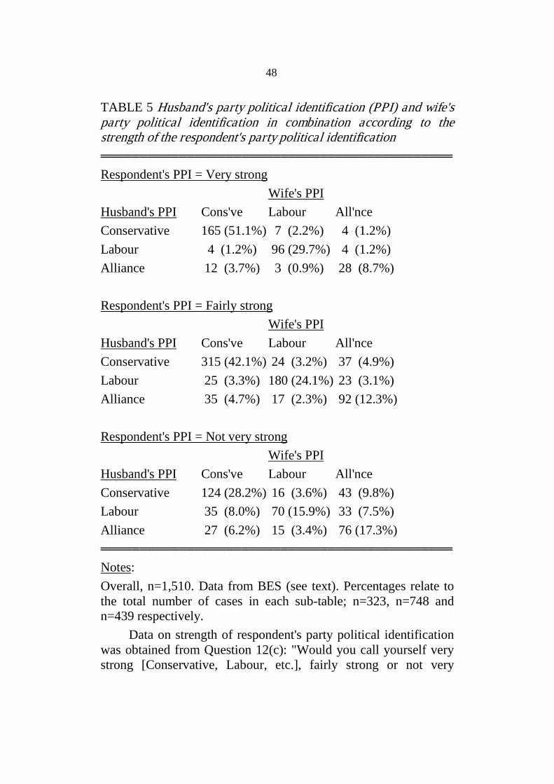
48

TABLE 5 Husband's party political identification (PPI) and wife's party political identification in combination according to the strength of the respondent's party political identification ═════════════════════════════════════════════

Respondent's PPI = Very strong



Labour 4 (1.2%) 96 (29.7%) 4 (1.2%) Alliance 12 (3.7%) 3 (0.9%) 28 (8.7%)

Respondent's PPI = Fairly strong



Labour 25 (3.3%) 180 (24.1%) 23 (3.1%) Alliance 35 (4.7%) 17 (2.3%) 92 (12.3%)

Respondent's PPI = Not very strong



Labour 35 (8.0%) 70 (15.9%) 33 (7.5%) Alliance 27 (6.2%) 15 (3.4%) 76 (17.3%) ═════════════════════════════════════════════

NotesOverall, n=1,510. Data from BES (see text). Percentages relate to the total number of cases in each sub-table; n=323, n=748 and n=439 respectively.

:

Data on strength of respondent's party political identification was obtained from Question 12(c): "Would you call yourself very strong [Conservative, Labour, etc.], fairly strong or not very

49

strong?". 81 cases included in Table 1 were omitted from Table 5 because they did not answer 12(c) or answered "Don't know".

50

TABLE 6 Respondent's party political (PPI) identification in combination with the party political identifications of various categories of relatives, friends and acquaintances ═════════════════════════════════════════════

Family members in respondent's household

(other than respondent's partner)

Family member's PPI Respondent's PPIConservative 193 (34.6%) 31 (5.6%) 28 (5.0%)


Labour 30 (5.4%) 154 (27.6%) 13 (2.3%) Alliance 30 (5.4%) 18 (3.2%) 60 (10.8%) Family members not in respondent's household

(other than respondent's partner)

Family member's PPI Respondent's PPIConservative 131 (28.7%) 42 (9.2%) 27 (5.9%)


Labour 28 (6.1%) 117 (25.7%) 16 (3.5%) Alliance 31 (6.8%) 27 (5.9%) 37 (8.1%)

Neighbours

Neighbour's PPI Respondent's PPIConservative 76 (35.5%) 10 (4.7%) 13 (6.1%)


Labour 22 (10.3%) 45 (21.0%) 11 (5.1%) Alliance 10 (4.7%) 9 (4.2%) 18 (8.4%)

Co-workers

Co-worker's PPI Respondent's PPIConservative 147 (23.7%) 77 (12.4%) 44 (7.1%)


Labour 58 (9.3%) 124 (20.0%) 23 (3.7%) Alliance 52 (8.4%) 63 (10.1%) 33 (5.3%)

51

Other friends

Other friend's PPI Respondent's PPIConservative 166 (28.2%) 65 (11.1%) 36 (6.1%)


Labour 35 (6.0%) 125 (21.3%) 25 (4.3%) Alliance 41 (7.3%) 51 (8.7%) 44 (7.5%) ═════════════════════════════════════════════

Notes: Data from BES (see text and Table 1). Percentages relate to the total number of cases in each sub-table; n=557, n=456, n=621, n=214, and n=588 respectively.

52

TABLE 7 The relationship between age and respondent's perception of the importance of "agreement on politics" to a successful marriage ═════════════════════════════════════════════ Very Fairly Not Very Not At All AgeUnder 35 6 (1.2%) 47 (9.7%) 262 (53.9%) 171 (35.2%)

Important Important Important Important

35 to 49 6 (1.4%) 49 (11.3%) 264 (61.0%) 114 (26.3%) 50 to 64 15 (4.2%) 44 (12.3%) 200 (55.9%) 99 (27.7%) 65 or over 14 (5.5%) 58 (22.8%) 136 (53.5%) 46 (18.1%) ═════════════════════════════════════════════

NotesData from BSAS (see text). Percentages in each row add up to 100%; n=1,531.

:

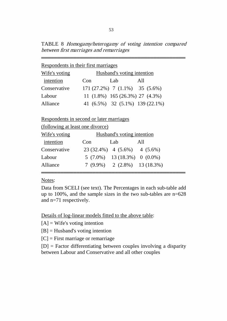
53

TABLE 8 Homogamy/heterogamy of voting intention compared between first marriages and remarriages ═════════════════════════════════════════════

Respondents in their first marriages Wife's voting

Husband's voting intention intention

Conservative 171 (27.2%) 7 (1.1%) 35 (5.6%) Con Lab All

Labour 11 (1.8%) 165 (26.3%) 27 (4.3%) Alliance 41 (6.5%) 32 (5.1%) 139 (22.1%) Respondents in second or later marriages (following at least one divorce) Wife's voting

Husband's voting intention intention

Conservative 23 (32.4%) 4 (5.6%) 4 (5.6%) Con Lab All

Labour 5 (7.0%) 13 (18.3%) 0 (0.0%) Alliance 7 (9.9%) 2 (2.8%) 13 (18.3%) ═════════════════════════════════════════════

NotesData from SCELI (see text). The Percentages in each sub-table add up to 100%, and the sample sizes in the two sub-tables are n=628 and n=71 respectively.

:

Details of log-linear models fitted to the above table[A] = Wife's voting intention

:

[B] = Husband's voting intention [C] = First marriage or remarriage [D] = Factor differentiating between couples involving a disparity between Labour and Conservative and all other couples

54

═════════════════════════════════════════════

Model Deviance [AB][AC][BC] 15.5 on 4 d.f. (p<.01)

Change in deviance

+ [CD] 4.3 on 3 d.f. (p>.05) 11.2 on 1 d.f. (p<.001) ═════════════════════════════════════════════

55

REFERENCES:

Becker G S. (1991): A Treatise on the Family (2nd edition). Cambridge:

Harvard University Press.

Blau P M. (1964): Exchange and Power in Social Life. New York: Wiley.

Blau P M. (1977): Inequality and Heterogeneity. New York: Free Press.

Blau P M, Beeker C, Fitzpatrick K M. (1984): `Intersecting Social Affiliations

and Intermarriage', Social Forces, 62.3: 585-606.

Blau P M, Blum T C, Schwartz J E. (1982): `Heterogeneity and Intermarriage',

American Sociological Review, 47.1: 45-61.

Brickell B, Huckfeldt R, Sprague J. (1988): Gender Effects on Political

Discussion: The Political Networks of Men and Women. Paper presented at the

annual meeting of the Midwest Political Science Association, Chicago.

Butler D, Stokes D. (1974): Political Change in Britain (2nd Edition).

London: Macmillan.

Catton W R, Smircich R J. (1964): `A Comparison of Mathematical Models

for the Effect of Residential Propinquity on Mate Selection', American

Sociological Review, 29.4: 522-529.

De Graaf N D, Heath A. (1992): `Husbands' and Wives' Voting-behaviour in

Britain: Class-dependent Mutual Influence of Spouses', Acta Sociologica, 35:

311-322.

Dean G, Gurak D T. (1978): `Marital homogamy the second time around',

Journal of Marriage and the Family, 40.3: 559-570.

Francis B, Green M, Payne C. (eds) (1993): The GLIM System: Release 4

Manual. Oxford: Oxford University Press.

56

Gallie D, Marsh C, Vogler C. (eds) (1994): Social Change and the Experience

of Unemployment. Oxford: Oxford University Press.

Gilbert G N. (1993): Analysing Tabular Data: Loglinear and Logistic Models

for Social Researchers. London: UCL Press.

Glenn N D, Hoppe S K, Weiner D. (1974): ` Social Class Heterogamy and

Marital Success: A Study of the Empirical Adequacy of a Textbook

Generalization', Social Problems, 21: 539-550.

Hayes B, Jones F L. (1992): `Marriage and Political Partisanship - Do Wives'

Characteristics Make a Difference?', Sociology, 26: 81-101.

Heath A, Curtice J, Jowell R, Evans G, Field J, Witherspoon S. (1991):

Understanding Political Change. Oxford: Pergamon Press.

Heath A, Jowell R, Curtice J. (eds) (1993): Labour's Last Chance: The 1992

Election and Beyond. Aldershot: Dartmouth.

Henry L. (1972): `Nuptiality', Theoretical Population Biology, 3: 135-152.

Himmelweit H, Humphreys P, Jaegar M, Katz M. (1981): How Voters Decide.

London: Academic Press.

Hollingshead A B. (1950): `Cultural factors in the selection of marriage

mates', American Sociological Review, 15: 619-627.

Huckfeldt R, Plutzer E, Sprague J. (1993): `Alternative Contexts of Political

Behaviour - Churches, Neighborhoods and Individuals', Journal of Politics,

55.2: 365-381.

Huckfeldt R, Sprague J. (1991): `Discussant Effects on Vote Choice:

Intimacy, Structure and Independence', Journal of Politics, 53.1: 122-158.

Jowell R, Witherspoon S, Brook L. (eds) (1987): British Social Attitudes: the

57

1987 report. Aldershot: Gower.

Kalmijn M. (1991a): `Status homogamy in the United States', American

Journal of Sociology, 97.2: 496-523.

Kalmijn M. (1991b): `Shifting boundaries: Trends in religious and educational

homogamy', American Sociological Review, 56: 786-800.

Kalmijn M. (1994): Àssortative mating by cultural and economic

occupational status', American Journal of Sociology, 100: 422-452.

Kerckhoff A C. (1963): `Patterns of homogamy and the field of eligibles',

Social Forces, 64: 289-297.

Kiernan K E. (1986): `Teenage Marriage and Marital Breakdown: A

Longitudinal Study', Population Studies, 40.1: 35-54.

Kingston P W, Finkel S E. (1987): Ìs There a Marriage Gap in Politics?',

Journal of Marriage and the Family, 49.1: 57-64.

Lampard R. (1992): An Empirical Study of Marriage and Social Stratification.

D.Phil. thesis: University of Oxford.

Mare R D. (1991): `Five decades of educational assortative mating', American

Sociological Review, 56: 15-32.

Morgan B S. (1981): À Contribution to the Debate on Homogamy,

Propinquity and Segregation', Journal of Marriage and the Family, 43: 909-

921.

Norusis M J. (1993): SPSS for Windows Advanced Statistics Guide Release

6.0. Chicago: SPSS Inc.

Peach C. (1974): `Homogamy, propinquity and segregation: a re-evaluation',

American Sociological Review, 39.5: 636-641.

58

Penn R D, Dawkins D C. (1983): `Structural Transformations in the British

Class Structure: A Log-Linear Analysis of Marital Endogamy in Rochdale

1856-196', Sociology, 17.4: 506-523.

Plutzer E, McBurnett M. (1991): `Family Life and American Politics: The

"Marriage Gap" reconsidered', Public Opinion Quarterly, 55.1: 113-127.

Ramsoy N R. (1966): Àssortative Mating and the Structure of Cities',

American Sociological Review, 31: 773-786.

Stier H, Shavit Y. (1994): Àge at marriage, sex-ratios, and ethnic

heterogamy', European Sociological Review, 10.1: 79-87.

Swaddle K M O, Heath A F. (1989): Òfficial and Reported Turnout in the

British General Election of 1987', British Journal of Political Science, 19:

537-570.

Tzeng M S. (1992): `The Effects of Socioeconomic Heterogamy and Changes

on Marital Dissolution for First Marriages', Journal of Marriage and the

Family, 54.3: 609-619.

Ultee W C, Luijkx R. (1990): Èducational Heterogamy and Father-to-Son

Occupational Mobility in 23 Industrial Nations: General Societal Openness or

Compensatory Strategies of Reproduction?', European Sociological Review,

6.2: 125-149.

university of warwick institutional repository article

Documents