university of toronto department of economics

University of Toronto Department of Economics

February 26, 2020

By Tongtong Hao, Ruiqi Sun, Trevor Tombe and Xiaodong Zhu

The Effect of Migration Policy on Growth, Structural Change,and Regional Inequality in China

Working Paper 659

The Effect of Migration Policy on Growth, Structural Change,and Regional Inequality in China

Tongtong Hao Ruiqi SunUniversity of Toronto Tsinghua University

Trevor Tombe Xiaodong Zhu∗

University of Calgary University of Toronto

Paper prepared for the 2019 Carnegie-Rochester-NYU Fall Conference on Public policyFirst version: October 2019. This Version: February 2020

Abstract

Between 2000 and 2015, China’s aggregate income quadrupled, its provincial income in-equality fell by a third, and its share of employment in agriculture fell by half. Workermigrationis central to this transformation, with almost 300 million workers living and working outsidetheir area or sector of (hukou) registration by 2015. Combining rich individual-level data onworkermigrationwith a spatial general equilibriummodel of China’s economy, we estimate thereductions in internal migration costs between 2000 and 2015, and quantify the contributionsof these cost reductions to economic growth, structural change, and regional income conver-gence. We find that over the fifteen-year periodChina’s internalmigration costs fell by forty-fivepercent, with the cost of moving from agricultural rural areas to non-agricultural urban onesfalling even more. In addition to contributing substantially to growth, these migration costchanges account for the majority of the reallocation of workers out of agriculture and the dropin regional inequality. We compare the effect of migration policy changes with other importanteconomic factors, including changes in trade costs, capital market distortions, average cost ofcapital, and productivity. While each contributes meaningfully to growth, migration policy iscentral to China’s structural change and regional income convergence. We also find the recentslow-down in aggregate economic growth between 2010 and 2015 is associated with smallerreduction in inter-provincial migration costs and a larger role of capital accumulation.

∗Xiaodong Zhu (corresponding author), University of Toronto and Tsinghua University, email [email protected]. Tongtong Hao, University of Toronto, email: [email protected]; Ruiqi Sun,Tsinghua University, email: [email protected]; and Trevor Tombe, University of Calgary, email:[email protected]. We would like to thank our discussant Jessica Leight, editor Laurence Ale, and participantsat the 2019 Carnegie-Rochester-NYU Conference on Migration Policy for valuable comments and suggestions. We alsothank Tsinghua-NBS Data Research Center for data support. The opinions and results of this paper does not representthe position of China’s National Bureau of Statistics.

1 Introduction

China’s economic growth since 2000 has been impressive. And although less well known, its rapidstructural change and large regional income convergence are no less remarkable. Between 2000and 2015, while the country’s aggregate GDP per worker quadrupled, the share of employment inagriculture fell in half and the income inequality across provinces fell by a third. Worker migrationis central to this transformation. The number ofworkerswho lived andworked outside their area ofhukou registration increased from around 110 million in 2000 to almost 300 million in 2015, mostlydue to changes in policies that made migration easier. In this paper, we quantify the impact ofmigration policy changes on China’s growth, structural change, and regional income convergence.

To accomplish this, we compile uniquely detailed data on production, capital, employment,trade, and migration in China. These data reveal four key facts concerning China’s structuralchange and regional convergence. First, there was significant regional convergence in real GDPper worker between 2000 and 2015. The variance of the cross-province (log) GDP per workerdeclined by a third, from 0.24 in 2000 to 0.15 in 2015. Second, over the same period, therewere little convergence in GDP per worker within the agricultural and non-agricultural sectors.Third, structural change was an important contributor to growth and convergence. The fraction ofemployment in agriculture fell from 53% in 2000 to 28% in 2015. The largest changes occurred inprovinces with lower initial levels of income, higher initial shares of agricultural employment, andlarger gap in labor productivity between the agricultural and non-agricultural sectors. Thereforereallocation of labor from agriculture to the non-agricultural sector resulted in larger increases inaggregate GDP perworker in poor provinces than in richer provinces and contributed significantlyto the convergence in aggregate income across provinces. Fourth, the structural change is closelyrelated to inter-provincial migration. Provinces with higher shares of employment in agriculturein 2000 had larger inter-provincial rural-urbanmigration flows. These facts suggest thatmigration-induced structural change is essential forChina’s growthand regional income convergencebetween2000 and 2015.

We bring our data to a rich yet tractable spatial equilibrium model of China’s economy toboth measure changes in migration costs and other frictions in China’s economy and to quantifytheir impacts on migration, structural change, growth, and regional income convergence. We findthat between 2000 and 2015 migration costs fell by forty-five percent, with the cost of movingfrom agricultural rural areas to non-agricultural urban ones falling even more. In addition tocontributing to growth, these migration cost changes account for the majority of the reallocationof workers out of agriculture and the drop in regional income inequality. We compare the effectof migration policy changes with other important economic factors, including changes in tradecosts, capital market distortions, average cost of capital, and productivity. While each contributesmeaningfully to growth, migration policy is central to China’s structural change and regionalconvergence. Finally, we find the slow-down in growth between 2010 and 2015 is associated withsmaller reduction in inter-provincial migration costs and a larger role of capital accumulationduring this five-year period.

1

Our model builds on recent developments in international trade. In particular, we extend theEaton and Kortum (2002) model to multi-sector as in Caliendo and Parro (2015) and incorporateboth imperfectly spatial and sector labor mobility as in Tombe and Zhu (2019). In addition, weallow for capital as an input in production and frictions in capital allocation across space andsectors. To better identify inter-sector migration costs, we also consider household preferencesthat are non-homothetic to control for the impact of income growth on rural-urban migration.

Our work contributes to the literature investigating the effect of China’s hukou system, andrecent reforms to it. Most recently, Zi (2019) explores the effect of internal frictions in China’slabor market on how trade liberalization improves welfare. In particular, hukou restrictions tendto dampen the gains from trade. On the other hand, Tian (2018) finds that the external tradeliberalization associated with China’s accession to WTO induced some of the migration policychanges and amplified the impact of external trade liberalization on internal migration in China.Estimating hukou restrictions at the prefecture-level, Ma and Tang (2019) find significant welfaregains from easing labor mobility restrictions. Finally, Kinnan et al. (2018) use China’s "sent-downyouth" program to identify exogenous effect of migration and find migration lowers consumptionvolatility and asset-holding. Our work is distinct not only methodologically, but also in that wefocus on a longer period of time, from 2000 to 2015, and examine the impact of migration policychanges on growth, structural change, and regional inequality at the same time in a unified modelthat with endogenous and frictional labor, capital, and production allocations.

Our work also builds on a large and growing literature quantifying the effects of internalmigration (Caliendo et al., 2017; Schmutz and Sidibe, 2018; Imbert and Papp, 2019; Heise andPorzio, 2019). Most recently, Bryan and Morten (2019) show that internal labor migration inIndonesia have significant implications for aggregate productivity there. Reducing migrationcosts to the U.S. level boosts aggregate productivity by 7.1%. Our work also connects with thoseinvestigating the link between trade and migration or structural change. Of particular relevancefor China, Fan (2019) demonstrates trade may exacerbate inequality, and Erten and Leight (2017)analyze the effect of China’s accession to WTO in 2001 on structural change at the local level.

By linking reallocation of labor across sectors to migration, we contribute to the large literatureon structural change (Herrendorf et al., 2014) and the agricultural productivity gap (Gollin et al.,2014). Given such gaps in labor productivity between sectors, shifting labor from agriculture tonon-agriculture can significantly boost aggregate productivity. We document that a central factorbehind China’s structural transformation is migration, both within and between provinces. Tobe clear, we are not the first to examine this link. Eckert and Peters (2018), for example, alsoexamine the interaction between migration and structural change. But, unlike for China, they findregional migration contributed little to the decline in the agriculture’s share of employment inthe United States. Finally, we build on the recent work of Alder et al. (2019), Comin et al. (2015),and Boppart (2014), by allowing for income effects (through non-homothetic preferences) to be adriver of structural change. We find income effects magnify the impact of reductions in migrationcosts on structural change and growth. We also show that ignoring income effects may lead one

2

to overestimate the initial level of, and reduction in, migration costs and therefore underestimateits contribution to growth and structural change.

Finally, our paper is closely related and build on thework by Tombe and Zhu (2019). We extendtheir work theoretically by incorporating into the model income effects through non-homotheticpreferences and physical capital as an input in production. We also extend their work empiricallyby extend their analysis of the impact of trade and migration on China’s growth between 2000 and2005 to a much longer and more recent period, from 2000 to 2015. Most important, we go beyondtheir analysis on aggregated GDP growth by studying the impacts of migration cost changes andother changes on both structural change and regional income inequality in China.

We begin our analysis with a detailed review of the data in Section 2, where we document keypatterns in China’s regional economic growth, structural change, and migration between 2000 and2015. With the data in hand, we develop a rich model of China’s economy that can be broughtto the data in Section 3. We then use this model to quantify the magnitude and consequence ofchanges in migration costs, trade costs, capital market distortions, and productivity. We documentthe results of this quantitative analysis in Section 4 before concluding in Section 5.

2 Migration, Structural Change, and Regional Income Convergence

In this section, we document large income disparity across provinces and between the agriculturaland non-agricultural sectors in China in 2000, and the significant regional income convergenceand rapid structural change between 2000 and 2015. We also provide evidence suggesting that thestructural change and regional income convergence are intimately related. We then discuss themigration policy changes and the resulting increases in internal migration as an important driverfor both the structural change and regional income convergence. First, however, we discuss brieflythe data we use for the paper.

2.1 Data

For our analysis, we combine three sources of data on internalmigration, internal and internationaltrade, and provincial economic accounts in China. We briefly list the important variables here, andprovide a more thorough description in the appendix.

Migration. Our migration data are from China’s population census. In addition to the 2000and 2005 census data used by Tombe and Zhu (2019), we also use the confidential micro data ofthe 2010 and 2015 population census of China.1 These census data provide detailed informationabout rural-urban and cross-province migration from 2000 to 2015.

Trade. We construct inter-provincial trade flows based on the inter-provincial input-outputtable for 2002, 2007, and 2012 from Li (2010), Liu et al. (2012), and Liu et al. (2018), respectively.

1These data are from NBS micro survey databases: 2010 China Population Census Mirco-database and 2015 1%Sample China Population Census Mirco-database.

3

Provincial GDP and Employment. We construct provincial GDP, capital stock, and employ-ment for agriculture andnon-agriculture basedmainlyon thedatapublished in theChinaStatisticalYearbook (CSY) by China’s National Bureau of Statistics (NBS). The construction methods for GDPand employment are the same as in Tombe and Zhu (2019). However, after 2010, the NBS no longerpublishes provincial employment by sector. For 2015, we therefore estimate provincial employ-ment based on the data published in the provincial yearbooks. We describe the full estimationprocedure in the appendix.

Provincial Capital Stock. The CSY reports nominal Gross Fixed Capital Formation (GFCF) byprovince but not by sector. However, it does report the fixed-asset investment by province andsector. We approximate each sector’s share of capital formation by using the sector’s share of totalfixed-asset investment. The real investment is nominal GFCF deflated using the province-specificinvestment price index reported in the CSY. We then construct capital stock using a perpetualinventory method assuming a depreciation rate of 7%. The average investment growth rates of thefirst ten years of a province are used to generate initial capital stock values for 1978. Our estimatesof annual real investment, less depreciation, are then used to calculate capital stock in subsequentyears.

2.2 Factor Return Dispersion across Provinces and Sectors

Tombe and Zhu (2019) document large differences in real labor income across provinces andbetween the agricultural and non-agricultural sectors in China in 2000, and they argue that animportant reason for these differences is the hukou system that imposes severe restrictions onworker mobility within China. Here we show the evolution of the distribution of real returns tolabor across provinces and sectors over the 15-year period after 2000.

Using data on real GDP, employment, and factor shares, the real marginal return to labor is

w jn � αβ j,l Y j

n

L jn

, (1)

where Y jn is real GDP of sector j in province n, L j

n is employment, β j,l is labor’s share of value-added, and α is the share of non-housing goods and services in GDP.We display the distribution ofreal marginal returns to labor for 2000, 2005, 2010, and 2015 in Figure 1a, which reveals persistentwithin-sector dispersion of labor returns across provinces and large gaps between agriculture andthe non-agriculture. Only in the last five years, between 2010 and 2015, did the within-sectordispersion in returns and the between sector gaps in returns decline slightly.

For comparison, we also report the distribution of returns to capital across provinces andsectors in Figure 1b. Specifically, the returns to capital in province n and sector j is

r j,kn � αβ j,k P j

nY jn

K jn

, (2)

4

Figure 1: Dispersion in Returns to Labor and Capital in China

(a) Real Returns to Labor

2010 2015

2000 2005

−3 −2 −1 0 1 2 −3 −2 −1 0 1 2

0

1

2

3

0

1

2

3

Log Relative Marginal Product of Labour

Density

Agriculture Non−Agriculture

(b) Nominal Returns to Capital

2010 2015

2000 2005

−3 −2 −1 0 1 2 −3 −2 −1 0 1 2

0

1

2

3

0

1

2

3

Log Relative Marginal Revenue Product of Capital

Density


Panel (a) displays the dispersion of returns to labor across provinces, by sector, from 2000 to 2015. Panel (b) displays the dispersion incapital wedges over the same period.

5

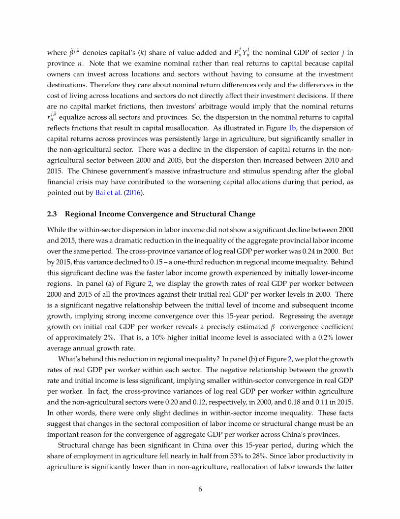
where β j,k denotes capital’s (k) share of value-added and P jnY j

n the nominal GDP of sector j inprovince n. Note that we examine nominal rather than real returns to capital because capitalowners can invest across locations and sectors without having to consume at the investmentdestinations. Therefore they care about nominal return differences only and the differences in thecost of living across locations and sectors do not directly affect their investment decisions. If thereare no capital market frictions, then investors’ arbitrage would imply that the nominal returnsr j,k

n equalize across all sectors and provinces. So, the dispersion in the nominal returns to capitalreflects frictions that result in capital misallocation. As illustrated in Figure 1b, the dispersion ofcapital returns across provinces was persistently large in agriculture, but significantly smaller inthe non-agricultural sector. There was a decline in the dispersion of capital returns in the non-agricultural sector between 2000 and 2005, but the dispersion then increased between 2010 and2015. The Chinese government’s massive infrastructure and stimulus spending after the globalfinancial crisis may have contributed to the worsening capital allocations during that period, aspointed out by Bai et al. (2016).

2.3 Regional Income Convergence and Structural Change

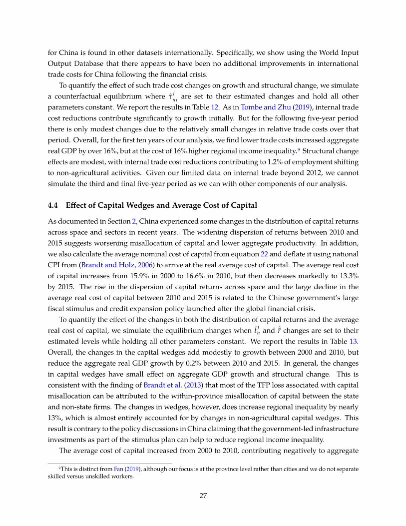
While thewithin-sector dispersion in labor income did not show a significant decline between 2000and 2015, therewas a dramatic reduction in the inequality of the aggregate provincial labor incomeover the same period. The cross-province variance of log real GDPperworkerwas 0.24 in 2000. Butby 2015, this variance declined to 0.15 – a one-third reduction in regional income inequality. Behindthis significant decline was the faster labor income growth experienced by initially lower-incomeregions. In panel (a) of Figure 2, we display the growth rates of real GDP per worker between2000 and 2015 of all the provinces against their initial real GDP per worker levels in 2000. Thereis a significant negative relationship between the initial level of income and subsequent incomegrowth, implying strong income convergence over this 15-year period. Regressing the averagegrowth on initial real GDP per worker reveals a precisely estimated β−convergence coefficientof approximately 2%. That is, a 10% higher initial income level is associated with a 0.2% loweraverage annual growth rate.

What’s behind this reduction in regional inequality? In panel (b) of Figure 2, we plot the growthrates of real GDP per worker within each sector. The negative relationship between the growthrate and initial income is less significant, implying smaller within-sector convergence in real GDPper worker. In fact, the cross-province variances of log real GDP per worker within agricultureand the non-agricultural sectors were 0.20 and 0.12, respectively, in 2000, and 0.18 and 0.11 in 2015.In other words, there were only slight declines in within-sector income inequality. These factssuggest that changes in the sectoral composition of labor income or structural change must be animportant reason for the convergence of aggregate GDP per worker across China’s provinces.

Structural change has been significant in China over this 15-year period, during which theshare of employment in agriculture fell nearly in half from 53% to 28%. Since labor productivity inagriculture is significantly lower than in non-agriculture, reallocation of labor towards the latter

6

Figure 2: Convergence in Provincial Real GDP per Worker, 2000 to 2015

(a) Growth Rate in Total Real GDP per worker.0

4.0

6.0

8.1

.12

.14

Avera

ge A

nnual G

row

th R

ate

, 2000−

2015

−1 −.5 0 .5 1

Log GDP/Worker in 2000, Relative to Average

log(GDP/worker)

(b) Growth Rate in Ag and Non-ag Real GDP per worker

.04

.06

.08

.1.1

2.1

4

Avera

ge A

nnual G

row

th R

ate

, 2000~

2015

−1 −.5 0 .5 1

Within Sector Log GDP/Worker in 2000, Relative to Average

Agriculture Non−agriculture

Displays the average annual growth rate in real GDP per worker in total, agriculture and non-agriculture from 2000 to 2015 againsteach province’s initial real GDP per worker in 2000. The negative relationship implies systematic convergence across provinces, whileconvergences are much smaller within either of the two sectors.

can increase a province’s overall labor productivity. Therefore, structural change can contributeto convergence in regional incomes if the pace of structural change was faster in poor provincesthan in rich provinces. And this is indeed the case. In panel (a) of Figure 3, we display thechange in the non-agricultural employment shares by province between 2000 and 2015. Provinceswith a relatively small non-agricultural sector in 2000 (and therefore lower average income) sawsignificantly larger employment shifts into this sector by 2015. Among those provinces with thesmallest initial non-agricultural employment share (at or below 40%), nearly one-third of totalprovincial employment moved out of agriculture. Among those with the largest initial non-agricultural employment share (at or above 80%), only 10% of workers switched. In addition, thereis a relationship between structural change and a province’s agricultural productivity gap (thegap between the agricultural and non-agricultural real GDP per worker). In panel (b) of Figure3, we plot the initial agricultural productivity gap in 2000 by province against each province’schange in the non-agricultural sector’s share of provincial employment between 2000 and 2015.With the exception of the six provinces with particularly low levels of structural change (threemunicipalities, and three peripheral regions), there is a positive relationship between the initialagricultural productivity gap and the pace of structural change.

To quantify in a simple way the degree to which structural change is driving regional con-vergence consider the following simple decomposition of a province’s aggregate real GDP perworker,

yn ,t � ya gn ,t + lna

n ,t ·(yna

n ,t − ya gn ,t

), (3)

where la gn ,t is province n’s non-agricultural employment share in year t and y j

n ,t is the real GDP perworker of sector j in province n and year t. Holding each sector’s real GDP per worker fixed at

7

Figure 3: Structural Change across Provinces in China, 2000 to 2015

(a) Convergence in Economic Structure

Beijing

ShanghaiTianjin

0.05

0.10

0.15

0.20

0.25

0.30

0.35

0.2 0.4 0.6 0.8 1.0

Non−agriculture employment share in 2000

Change in N

on−

Ag. E

mp. S

hare

, 2000−

2015

(b) Agricultural Productivity Gap and Structural Change

Beijing

Heilongjiang

Liaoning ShanghaiTianjin

Xinjiang

0.05

0.10

0.15

0.20

0.25

0.30

0.35

0.5 1.0 1.5 2.0

Nonag−to−Ag Real GDP per Worker Gap in 2000

Change in N

on−

Ag. E

mp. S

hare

, 2000−

2015

Panel (a) and (b) displays the change in the non-agricultural sector’s share of provincial employment between 2000 and 2015 againstthe initial share in 2000 and the agricultural productivity gap in 2000, respectively.

their 2000 levels, we calculate the counterfactual real GDP in province n as

yn ,t � ya gn ,2000 + lna

n ,t ·(yna

n ,2000 − ya gn ,2000

). (4)

We find the variance of ln( yn) falls by one-quarter when only lnan ,t is changing over time as in

the data. Our simple back-of-the-envelope calculation therefore suggests that structural changeaccounts for two-thirds of the observed convergence between China’s provinces.

Of course, this simple calculation ignores potential endogenous relationships between the laborreallocation and the labor productivity in the two sectors, which we will take into account in ourquantitative analysis of a full general equilibriummodel later. The simple calculation also does nottell us what drives the structural change. Next, we present evidence that worker migration fromagriculture to non-agriculture, both within- and between-provinces, can be an important driver ofthe structural change in China.

2.4 Internal Migration in China

Before turning to the data on migration and structural change, we first provide a summary ofChina’s internal migration policy and recent changes to it. The Chinese government formallyinstituted a household registration or hukou system in 1958 to control labor mobility. Chan (2019)provides a detailed and up-to-date discussion of the system and its reforms. Briefly, each Chinesecitizen is assigned a hukou, classified as "agricultural (rural)" or "non-agricultural (urban)" in aspecific location. Individuals need approvals from local governments to change the category(agricultural or non-agricultural) or location of hukou, and it is extremely difficult to obtain suchapprovals. Prior to 2003, workers without local hukou had to apply for a temporary residencepermit. As the demand for migrant workers in manufacturing, construction, and labor intensive

8

Table 1: Worker Migration in China, 2000-2015

Intra-Provincial Inter-Provincial2000 2005 2010 2015 2000 2005 2010 2015

Total Migrant Stock 101.5 132.6 176.2 215.7 29.7 47.0 79.2 90.2

Share of Employment (%)

Total Migrants 14.1 17.8 22.9 28.0 4.1 6.5 10.3 11.7Ag-to-Nonag Migrants 13.0 16.5 21.6 25.5 3.3 5.2 8.6 7.0

Non-migrant Ag Workers 63.0 55.5 46.3 31.6 63.0 55.5 46.3 31.6Note: Displays the number of workers living and working outside their area of hukou registration. The first row is inmillions. The last three rows are shares of total employment.

service industries increased, many provinces, especially the coastal provinces, eliminated therequirement of temporary residencepermit formigrantworkers after 2003. Therewas also anation-wide administrative reform in 2003 that greatly streamlined the process for getting a temporaryresidence permit in other provinces. These policy changes made it much easier for a worker toleave their hukou location and work somewhere else as a migrant worker. However, even with atemporary residencepermit,migrantworkerswithout local hukouhave limitedaccess to local publicservices and face higher costs for health care and for their children’s education. In the late 1990s, afew locales began experimenting with eliminating the distinction between local agricultural/non-agricultural populations, providing all local residents with a resident hukou entitling them equalaccess to local public services. This was eventually formalized and extended to the whole nationin 2014. At the same time, however, the government has tightened the requirement for grantinghukou to migrants in the first- and second- tiered cities. So, over time, it has become easier for arural migrant worker to obtain hukou in a local urban area in lower tiered cities, but it has becomeharder in recent years for them to move to large coastal cities due to the stricter restrictions there.

Based on population census data, we report in Table 1 both inter-provincial and intra-provincialmigration in China for the years of 2000, 2005, 2010, and 2015.2 As a reference, we also reportthe share of workers who are non-migrant agricultural workers. A worker is defined as an inter-provincialmigrant if theyworkedoutside their province of hukou registration. And they aredefinedas an intra-provincial migrant if they workedwithin their province of registration but outside theirsector of hukou registration. Our definition of intra-provincial migration is broader than usual.Some workers with agricultural hukoumay work in non-agriculural jobs locally (within the villageor township of their hukou registration) and they are classified as intra-provincial migrant workers.We choose this definition because we find from the 2005 mini-census data that the average incomeof these local "migrant workers" is more than 2.5 times as high as that of the local farmers. Thissuggests that there are significant frictions for rural workers switching sectors locally. In ourrobustness analysis later, we will consider a stricter definition of migrant workers.

2Themigration stocks are calculated from the data onmigrant shares from the census data and the total employmentdata in the China Statistics Yearbooks. See appendix for details.

9

Figure 4: Migration and Structural Change

0.0

5.1

.15

.2

Inte

r−pro

vin

cia

l A

g to N

a M

igra

tion S

hare

in 2

015

.2 .4 .6 .8 1

Non−ag Employment Share in 2000

The figure displays the fraction of initially agricultural workers that now work in non-agriculturalsectors, overall and out of province. This captures the relationship between migration and structuralchange.

As documented by Tombe and Zhu (2019), the relaxation of hukou restrictions on migrationbetween 2000 and 2005 resulted in significant increases in both intra- and inter-provincial migra-tion.3 The general trend seems to have continued between 2005 and 2015, with the intra- andinter-provincial migrant workers’ shares of total employment increased from 17.8% and 6.5%,respectively, in 2005, to 28% and 11.7% in 2015. Between 2010 and 2015, however, the increasein inter-provincial migration slowed significantly, and the cross-provincial rural-urban migrantworkers’ share of total employment in 2015 is actually lower than that in 2010. In contrast, within-province rural-urban migration continued to increase significantly through 2015. These patternsare consistent with the policy changes adopted by the Chinese government after 2010 that havemade moving to top tier cities, the destinations of much of the inter-provincial migration, muchharder for people with rural hukou and, at the same time, encouraged local urbanization in poorinland and western provinces.

To see the impact of migration on structural change, in Figure 4, we plot for all the provincestheir initial share of employment in agriculture in 2000 against their share of all the workers withagricultural hukou in that province who work in the non-agricultural sector in another province in2015. We can see that provinces with higher shares of initial agricultural employment tend to havea larger proportion of workers move out of agriculture and into the non-agricultural sector outside

3Our estimated migration stocks are slightly different from those reported by Tombe and Zhu (2019) because wenow use more detailed sample weights provided by the NBS.

10

their hukou registration provinces in 2015. Simply put, reductions in the share of employment inagriculture in poor provinces are associated with intra-provincial out-migration of farmers.

In summary, the facts we document in this section suggest that migration policy changes andthe associated increases in migration have important effects on structural change and regionalincome convergence in China between 2000 and 2015. We now turn to our main analysis thatprecisely quantifies these effects using a spatial general equilibriummodel of trade and migration.

3 A Spatial Model of Trade and Migration

The focus of ourmodel is on quantifying the impact ofmigration cost changes on growth, structuralchange, and regional income convergence in China between 2000 and 2015. During this period,however, there were changes in trade costs, capital costs, and province-sector specific TFPs thatcould also affect growth, structural change, and regional income convergence in China. To identifythe impact of migration cost changes, we use a tractable quantitative model of trade andmigrationbased on the one used in Tombe and Zhu (2019), but extended to allow for capital in productionand capital market frictions. In addition, since the recent literature on structural change haveemphasized the importance of income effect, we further extend the model with non-homotheticpreferences to allow for income effects on structural change. The details of the model follow.

3.1 Individual Agents

There are N provinces in China and 1 region representing the rest of the world. There are twotypes of agents in our model: registered workers with local hukou, and migrant workers withoutlocal hukou. We denote the number of workers in each province and sector as L j

n and the numberof individuals registered in each province and sector as L j

n . As workers are mobile, the number ofworkers in a province need not equal the number of individuals holding a hukou registration there.The number of hukou registrants in a province and sector is fixed.

Following Muellbauer (1975) and, more recently, Boppart (2014) and Alder et al. (2019), in-dividual preferences are characterized by the Price Independent Generalized Linearity (PIGL)specification, with indirect utility function

V jn(q) �

1ε

e j

n(q)(Pa gφ

n Pna1−φn

)αr j,h1−α

n

ε

− Bγ

(Pa g

n

Pnan

)γ, (5)

for individuals of type-q (eithermigrants ornon-migrant locals)with earnings e jn(q). Theparameter

γ governs the sensitivity of expenditure shares to changes in relativeprices, ε governs the sensitivityof expenditure shares to changes in income, and B ≥ 0 governs the importance of relative prices.This specification is useful for aggregating individuals with differing levels of income within each

11

region in a tractable manner.4 And although a closed form representation of the direct utilityfunction does not exist, it includes the standard Cobb-Douglas preferences as a special case whenB � 0 and ε � 1. The implied aggregate shares of spending allocated to goods and housing areprovided in the following proposition.

Proposition 1 The fraction of aggregate expenditures allocated to the agricultural good, non-agriculturalgood, and housing in province n and region j are

Ψj,a gn � αφ + B

(Pa g

n

Pnan

)γ e j

n(Pa gφ

n Pna1−φn

)αr j,h1−α

n

−ε

, (6)

Ψj,nan � α(1 − φ) − B

(Pa g

n

Pnan

)γ e j

n(Pa gφ

n Pna1−φn

)αr j,h1−α

n

−ε

, (7)

Ψj,hn � 1 − α (8)

where e jn �

[∑q e j

n(q)−εωjn(q)

]−1/εis the average income across all individuals, and ω j

n(q) ∝ e jn(q)L

jn(q)

is the weight of type-q workers in total income in (n , j).

Proof: See the appendix.These spending shares imply that as income grows large, the share allocated to the purchase of

agricultural goods converges to αφ from above. Similarly, the share allocated to non-agriculturalgoods converges to α(1− φ) from below. And the share allocated to housing is fixed. In the rest ofthe paper, we will consider the case when B � 1.

In certain situations, it is convenient to represent utility as a function of real incomes andexpenditure shares. Using equation 6 to substitute for relative prices in equation 5, one can writethe utility of an individual with real income v j

n(q) allocating a share ψ j,a gn (q) of their income to

agriculture goods as

V jn(q) �

(1ε−ψ

j,a gn (q) − αφ

γ

)v j

n(q)ε . (9)

This expression will prove particularly useful in the calibration and quantitative analysis to come,as it maps directly to data on expenditure shares and real incomes.

4An alternative choice is the nonhomothetic CES preferences (Comin et al., 2015). However, in this case, we cannotaggregate consumption demand of the migrants and non-migrants into the demand of a representative agent. It isprimarily for this reason that we opt for the PIGL specification.

12

3.2 Production and Trade

Within each sector, final goods are produced as aggregates over a continuumof individual varietiesν ∈ (0, 1) according to the CES technology

Y jn �

(∫ 1

0y j

n(ν)(σ−1)/σdν)σ/(σ−1)

, (10)

where σ is the elasticity of substitution across varieties. For each variety, producers use labor,capital, land and a composite intermediate good to produce output using the followCobb-Douglastechnology,

y jn(ν) � z j

n(ν)ljn(ν)β

j,lk j

n(ν)βj,k

h jn(ν)β

j,h∏

s�{a g ,na}m j

n(ν)βj,s, (11)

where β j,l + β j,k + β j,h +∑

s βj,s � 1. This implies the marginal cost of production is inversely

proportional to productivity and proportional to the cost of an input bundle

c jn ∝ (w

jn)β

j,l (r j,kn )β

j,k (r j,hn )β

j,h∏

s�{a g ,na}(Ps

n)βj,s. (12)

While a sector’s composite output is not tradeable, individual varieties are. Trade is costly,however, and τ j

ni units must be shipped for one to arrive at the destination. Trade within a regionis costless, and therefore τ j

nn � 1. Together with the marginal costs of production, the price forsector j varieties produced in region i and shipped to region n is

p jni(ν) � τ

jni c

ji /z

ji (ν). (13)

The overall pattern of consumer and business intermediate spending across possible suppliersfrom either their own region or from others is such that the cost of a sector’s aggregate compositegood is minimized. As demonstrated by Eaton and Kortum (2002), if productivity is distributedFréchet, with CDF given by F j

n(z) � e−T jn z−θ , with variance parameter θ and location parameter T j

n ,then the share of total sector j spending allocated by buyers in region n to producers in region i is

πjni ∝ T j

i

(τ

jni c

ji

P jn

)−θ, (14)

where the price index P jn is

P jn ∝

[N+1∑i�1

T ji

(τ

jni c

ji

)−θ]−1/θ

. (15)

In both equations 14 and 15, the constant of proportionality is common across regions and sectors.Trade shares from equation 14 determine total sales of each sector in all regions. Given total

13

spending X jn by consumers and firms in region n on goods from sector j, total revenue is

R jn �

N+1∑i�1

πjinX j

i , (16)

which implies intermediate demand by firms is β j,s R jn . Combined with final demand spending by

consumersΨs , jn e s

nLsn , total spending on good j by consumers and firms in region n is therefore

X jn �

∑s∈{a g ,na}

Ψs , jn e s

nLsn +

∑s∈{a g ,na}

βs , jRsn . (17)

3.3 Incomes from Employment, Land, and Capital

Workers earn income from work and, for some, from their claims to land and capital returns.Broadly consistent with China’s institutional setting, we presume only local non-migrant individ-uals receive income from land and capital in their region. Thus, the income of migrant workers isonly their wage w j

n while the income of non-migrant locals is w jnδ

jn , where δ j

n > 1 represents theratio of total income including rebate of land and capital income to labor income. We show howto determine the equilibrium value of δ j

n below.Total rebates in each region combine a number of sources. Total spending on land, for housing

by individuals and as an input to production by firms, equals total land rebates. Specifically, ifsectoral sales are R j

n then spending on land inputs is β j,hR jn and if consumer income is e j

nL jn then

their spending on housing is (1− α)e jnL j

n . All together, if total land supply in a given province andsector is H j

n then total land income is

r j,hn H j

n � β j,hR jn + (1 − α)e j

nL jn . (18)

Similarly, spending on capital by producers is proportional to their total sales β j,kR jn � r j,k

n K jn . Total

income from all sources is therefore

e jnL j

n � w jnL j

n + β j,hR jn + (1 − α)e j

nL jn + β j,kR j

n , (19)

which implies average per capita income is

e jn � w j

n

(β j,l + β j,h + β j,k

αβ j,l

)≡ w j

n

λ j , (20)

where λ j � αβ j,l/(β j,l +β j,h +β j,k) < 1. Note this follows because a sector’s wage bill is a fixed shareβ j,l of its revenue. Conveniently, average per capita income is a fixed proportion to wages. We alsosolve for the income premium to non-migrants, captured by δ j

n , in the following proposition.

Proposition 2 Given wages w jn and migration shares m js

ni , per capita income of non-migrant local workers

14

in province n and sector j is δ jn w j

n where

δjn � 1 +

1 − λ j

λ j

L jn

L j jnn

(21)

where L j jnn is the population of non-migrant workers.

Proof: See the appendix.To simplify some of the expressions to come, let δ js

ni equal δjn if n , i or j , s and 1 otherwise.

3.4 Capital Market Clearing Condition

Capital market clearing is national in scope. That is, total capital demanded by producers in allsectors andprovincesmust add to the total capital supply K. As each sector in each region optimallychooses a quantity of capital demanded to equate the marginal revenue product of capital to thecost of capital they face, which reflects the average cost of capital common to all sectors and thecapital wedge facing that particular sector and province. Specifically, given capital wedges t j

n suchthat β j,kR j

n/Kjn � r j,k

n ≡ r/(1 − t jn), we have

N∑n�1

∑j∈{a g ,na}

1 − t jn

rβ j,k

β j,lw j

nL jn � K , (22)

since β j,lR jn � w j

nL jn hold for all n and j. This expression illustrates that, all else equal, a reduction

in the average cost of capital r reflects a rising aggregate supply K. This will prove to be animportant component of recent growth in China.

To complete themodel, we next solve for the equilibriummigration shares m jsni and employment

L jn in each province and sector.

3.5 Worker Mobility Across Provinces

Workers in China choose where to live (andwork) to maximize welfare. Workers are heterogenousin their taste for different regions and sectors, and face costs when living outside their region ofhukou registration. Labor is perfectly mobile across sectors in the rest of the world. When decidingin which province and sector to work, an individual from province n and sector j compares thepotential utility level in all destinations V js

ni , the migration costs between (n , j) and (i , s), and thepotential loss of land and capital income reflected in δ js

ni . From equation 9, V jsni is as follows

V jsni �

(δ

jnε

ε −ψ

j,a gn −αφγ

)v j

nε

i f n � i , j � s(1ε −

ψj,a gn −αφγ

)v j

nε

i f n , i , j , s(23)

15

where ψ j,a gn and v j

n are the spending share on agriculture goods and real income perworker formi-gratingworkers living in province n and sector j. In addition, let worker preferences over locationsbe captured by zs

i , which is distributed identically and independently across workers and followsa Fréchet distribution with variance parameter κ. Workers then choose the destination (i , s) tomaximize zs

i V jsni /µ

jsni . Solving for the share of workers that opt to move to each possible destination

is straightforward. We provide the equilibrium migration shares in the follow proposition:

Proposition 3 Given indirect utilitiesV jsni , migration costs µ js

ni , and a Fréchet distribution of idiosyncracticpreferences Fz(x), the fraction of workers registered in province n and sector j that migrate to province i andsector s is

m jsni �

(V js

ni /µjsni

)κ∑

s′∈{a g ,na}∑N

i′�1

(V js′

ni′ /µjs′

ni′

)κ (24)

where V jsni is indirect marginal utility from equation 9.

Proof: See the appendix.This expression for migration shares conveniently summarizes the pattern of inter-provincial

and inter-sectoralmoves byworkers. Note that the parameter κmeasures the elasticity ofmigrationwith respect to utility. From equation 9, we can see that the elasticity of migration with respect toreal income is εκ, which can be directly estimated from the data. So, for any given value of ε, wecan use the estimated income elasticity of migration to infer the utility elasticity κ.

Finally, given the migration shares and hukou registrations, total employment in each provinceand sector is

L jn �

N∑i�1

∑s∈{a g ,na}

ms jin Ls

i , (25)

and the number of non-migrant locals is L j jnn � m j j

nn L jn .

4 Quantitative Analysis

We now bring the full model to data. We first calibrate the values of the time-invariant modelparameters. Given these parameter values and for each of the four years (2000, 2005, 2010, and2015), we calibrate the migration costs, trade costs, capital wedges, the average cost of capital, andthe province-sector specific TFPs so that the model matches trade, migration, capital stocks, andreal GDP in the data. This provides estimates of trade and migration costs, capital market distor-tions, and average cost of capital over time. To quantify their effect on overall economic activityand regional income inequality in China, we simulate the model under various counterfactualexperiments detailed below.

16

Table 2: Model Parameters and Initial Equilibrium Values

Parameter Value Description(βa g ,l , βna ,l) (0.27, 0.19) Labor’s share of output(βa g ,k , βna ,k) (0.06, 0.15) Capital’s share of output(βa g ,h , βna ,h) (0.26, 0.01) Land’s share of output(βa g ,a g , βna ,a g) (0.16, 0.04) Agricultural input’s share of output(βa g ,na , βna ,na) (0.25, 0.61) Nonagricultural input’s share of output

α 0.87 Goods’ expenditure shareφ 0 Agriculture goods’ share in price indexγ 0.30 Price-effect in expenditure sharesε 0.70 Income-effect in expenditure sharesΨ

j,a gn Data Agriculture goods’ expenditure shareθ 4.0 Elasticity of tradeκ 2.14 Heterogeneity in location preferencesπ

jni Data Trade shares

m jsni Data Migration shares

L jn Data Initial hukou registrations

Notes: Displays the main model parameters and the initial equilibrium values for endogenousobjects set to match data prior to solving the model in relative changes. See text for details.

4.1 Calibration of Time-Invariant Parameters

To ease the calibration and quantitative exercise, we solve the model in relative changes as in Dekleet al. (2007). This requires a number of equilibrium objects be set equal to data in the initial periodequilibrium, which in our case is the year 2000. The key objects here are the initial trade shares π j

ni ,migration shares m js

ni and registeredworkers. In particular, we use themigration sharematrix fromthe 2000 census and the employment by province and sector from the 2000 CSY to back out theinitial registered workers by province and sector,5 and keep them constant for all the quantitativeanalysis.6

We describe the calibration of each time-invariant model parameter in detail below, and reportthe relevant values in Table 2. Production function parameters are calculated to match the shareof sector output going to each type of input, as reported in our Input-Output data. The share ofconsumer expenditures allocated to housing is set to the average share reported in the China Sta-tistical Yearbook for rural (15%) and urban (11%) households. Agriculture’s share of expendituresin the initial equilibriumΨ j,a g

n is also from the data.Some model parameters correspond to empirical elasticities and other moments in the data.

We set their values to correspond to common values from the literature, and explore the sensitivity

5We use this approach to eliminate the gaps in employment between the census and CSY. The Chinese populationcensus and theNBS labor survey, the source of the employment data inCSY, use different surveymethods in enumeratingagricultural and non-agricultural employment. The census provides more accurate information about migration, butless accurate information on employment. We discuss this in more detail in the data appendix.

6For robustness, we also report the results with registeredworker changing for each five year period in the appendix,and our main results do not change much.

17

of our results to alternative values in the appendix. In particular, the elasticity of migration flowsto real income differences εκ is set to match the elasticity of 1.5 estimated by Tombe and Zhu(2019). Given our value for ε (described in a moment), this implies κ � 2.14. The elasticity oftrade flows with respect to trade costs θ is set to 4, in line with evidence from international trade.Following evidence from Tombe (2015), we use the same elasticity for both the agricultural andnon-agricultural sectors. Turning to consumer preference parameters, we set the strength of theincome and price effects in consumer expenditure shares to 0.7 and 0.3, respectively. The formeris in line with Alder et al. (2019) who finds ε ∈ (0.68, 0.76) for the United States across differenttime periods, but the latter is less precise. They also find values for ε in the UK (0.76), Canada(0.34), and Australia (1.0). There are other researchers who choose lower values for ε. For example,Boppart (2014) sets it to 0.22 and Eckert and Peters (2018) set it to 0.35. In China, although we donot rigorously estimate ε here, a regression of log-expenditure shares on log-income suggests avalue between 0.8 and 1.0. We opt for 0.7. The value of γ is set to 0.3, close to Boppart (2014)’sestimate of 0.41 and Eckert and Peters (2018)’s of 0.32. We show that our results are robust toalternative values for ε and γ in the appendix. Finally, the long-run share of spending allocatedto agriculture φ is set to 0, which simplifies equation 9 with very little quantitative effect on ourresults, as we demonstrate in the appendix.

4.2 Size and Impact of Migration Cost Reductions

4.2.1 Estimating Migration Cost Changes

With the calibrated parameters and our data on real incomes, employment, hukou registrations,and migration shares, we infer the full matrix of bilateral migration costs between provinces andsectors. Specifically, we solve for migration costs µ js

ni such that equation 24 holds, and fromequation 9, we have

µjsni �

V jsni

V j jnn

(m js

ni

m j jnn

)−1/κ

�1/ε − (ψs ,a g

i − αφ)/γ

δjεn /ε − (ψ

j,a gn − αφ)/γ︸︷︷︸

NonhomotheticPre f erences

(vs

i

v jn

) ε︸︷︷︸

Real IncomeGap

(m js

ni

m j jnn

)−1/κ

(26)

We use data on real GDP by province and sector to estimate real wages and land and capitalrebates, using equation 20, and data on consumption shares by province and rural or urban areato estimate agricultural spending shares. With these estimates in hand, we report the resultingmigration-weighted average migration costs in Table 3.

The average of the direct migration costs µ jsni is reported in the second row of the table. It was

substantial in 2000, but fell by 45% over the next 15 years. The first row of the second panel in thetable show that the average of rural-to-urban or agriculture-to-nonagriculture migration costs waseven higher in 2000 and also fell more, by 61% between 2000 and 2015. Note that migration costsof less than one do not imply migrants earn more than non-migrants, since these costs are net of

18

Table 3: Average Migration Costs in China

Average Cost Relative to 2000Year 2000 2005 2010 2015 2005 2010 2015

Overall, Including δ jn 3.96 3.59 2.90 2.17 0.91 0.81 0.75

Direct migration costs µ jsni 1.75 1.63 1.31 0.96 0.93 0.75 0.55

Agriculture to Nonagriculture µ jsni

Overall 2.68 2.23 1.57 1.04 0.83 0.58 0.39Within Provinces 2.25 1.87 1.32 0.87 0.83 0.59 0.39Between Provinces 11.38 9.55 5.95 4.88 0.84 0.52 0.43

Between Province µ jsni

Overall 9.14 8.00 5.54 3.68 0.88 0.61 0.40Within Agriculture 11.61 13.48 10.62 14.99 1.16 0.91 1.29Within Nonagriculture 5.67 5.06 4.14 1.92 0.89 0.73 0.34Note: Displays the weighted-average migration cost for various years and various types of migration moves.The last three columns display the migration costs in each year relative to 2000. All migration costs displayedare exclusive of the foregone returns to land and capital that accrue only to non-migrant locals, except for thefirst row that includes this in the average.

the foregone land and capital returns due to their living outside their hukou region. The first rowof the table shows the overall average cost of moving that includes the foregone returns to landand capital. It was roughly equivalent to three-quarters of annual income in 2000. By 2015, theoverall average cost declined by 25% and was roughly equivalent to half of annual income. Overthe three 5-year periods, the magnitude of the migration cost reductions generally increased overtime, but the between-province rural-to-urban migration cost reduction between 2010 and 2015 islower than the reduction between 2005 and 2010. This is most likely due to the strict populationcontrol policy implemented after 2010 in all the first-tier and some second-tier cities.

4.2.2 Quantifying the Effect of Migration Cost Changes

To quantify the effect of these migration cost changes, we start from the 2000 initial equilibriumand solve for relative changes in the model where change in µ js

ni are set to their estimated valuesand all other model parameters are held constant. Though we report only the average changes inmigration costs in Table 3, we simulate the effect of changes in migration costs across all bilateralprovince-sector pairs. Table 4 reports the resulting changes in aggregate real GDP, provincialincome inequality, and agriculture’s employment share.

Changes in internal migration costs have significant effects on aggregate economic activity,regional income inequality, and structural change. The top three rows of Table 4 show the effectof all estimated migration cost changes. First, as a result of these changes, the aggregate realGDP increases by 4.4%, 5.9%, and 6.9%, respectively, over the three 5-year periods ending in 2005,

19

Table 4: Effect of Lower Migration Costs, 2000-2015

Five-Year Growth (%)for Year Ending Cumulative Homothetic

Changes in All Migration Costs 2005 2010 2015 Effect Preferences

Aggregate Real GDP Growth 4.3 5.9 6.9 18.0 12.6Provincial Income Inequality -10.6 -14.4 -19.2 -38.2 -35.2Agriculture’s Employment Share -3.2 -5.5 -7.7 -16.3 -13.8

Changes in Ag to Non-ag, Within-Province Migration Costs

Aggregate Real GDP Growth 2.5 2.9 3.8 9.4 5.6Provincial Income Inequality -1.9 -3.4 -7.2 -12.1 -5.7Agriculture’s Employment Share -2.3 -3.6 -6.1 -12.0 -10.0

Changes in Ag to Non-ag, Between-Province Migration Costs

Aggregate Real GDP Growth 1.9 3.5 2.5 8.1 6.8Provincial Income Inequality -6.9 -11.3 -13.0 -28.2 -30.3Agriculture’s Employment Share -1.0 -2.4 -2.0 -5.4 -5.0Note: Displays the effect of changing migration costs in each of the three five-year periods ending in 2005, 2010, and 2015.The cumulative effects with benchmark model and homothetic-preference model are reported in the last two column. Chang-ing ag-to-nonag migration costs affects move between agriculture and non-agriculture only. This is further decomposed into itswithin-province and between-province components. The change in provincial income inequality is reported as the change in thevariance of log real GDP per worker across provinces. The change in agriculture’s share of national employment is reported asthe percentage point change.

2010, and 2015. The cumulative effect over the 15-year period is an 18% increase in the aggregatereal GDP. The second and third panel of Table 1 show separately the impact of the reductions inwithin- and between-province agriculture to non-agriculture migration costs. They increase theaggregate GDP by about similar amount, 9.4% and 8.1%, respectively. To put the magnitude of theaggregate GDP increase (or aggregate labor productivity increase since we have normalized thetotal employment to one) in perspective, we compare our results to two recent studies on the gainsfrom reducing spatial misallocation in some other economies. Fajgelbaum et al. (2019) estimatethat a hypothetical complete elimination of state business tax wedges in the US would result in 0.6%increase in welfare for the US, and Bryan and Morten (2019) estimate that a hypothetical reductionof the migration costs in Indonesia to the US levels would result in 7% increase in the aggregatelabor productivity in that economy. In contrast, the 18% increase in the aggregate GDP in Chinais a result of the estimated actual reductions in migration costs in China. There was significantspatial misallocation in China due to its hukou system that imposed severe restrictions on China’sinternal labor mobility and therefore the gain from relaxing those restrictions is large. Despitethe reduction in migration costs, however, the labor mobility in China is still much lower thanthat in the US. Table 1 shows that the inter-provincial migrant workers as a percentage of totalemployment was only 11.7% in 2015, much lower than the share of workers in the US who workout of their state of birth, which has been around one third.

20

Figure 5: Real GDP/Worker Gains from Lower Migration Costs, 2000 to 2015

Heilongjiang

Xinjiang

ShanxiNingxia Shandong

Henan Jiangsu

AnhuiHubei

Zhejiang

JiangxiHunan

Yunnan

Guizhou Fujian

Guangxi Guangdong

Hainan

Jilin

Liaoning

Tianjin

Qinghai

Gansu

Shaanxi

InnerMongolia

Chongqing

Hebei

Shanghai

Beijing

Sichuan

−20% 0% 20%

Change in RealGDP per Worker:

Displays the gains in provincial real GDP per worker, across all sectors, in response to changes in migration costsbetween 2000 and 2015. Blue illustrates increases while red illustrates decreases.

The second row of Table 4 shows that the migration cost reductions also significantly reducedregional inequality. Overall, the variance of log real GDP per worker across provinces falls byover one-third. We plot the income gains across each of China’s provinces as a choropleth inFigure 5 to illustrate that the lower income interior regions gain notably more from the migrationcost reductions than the coastal ones and therefore the decline in regional income inequality.The second and the third panel of the table show that, not surprisingly, the between-provincemigration cost reductions contribute much more to the decrease in provincial income inequalitythan the within province migration cost reductions, about two-third vs. one-third.

The third row of Table 1 shows that about 16% of total employment shifts from agriculture tonon-agricultural activities as a result of the change inmigration costs. And the second and the thirdpanel of the table show that thewithin-provincemigration cost reductions aremore important thanthe between-provincemigration cost reductions in generating the decline in the agriculture’s shareof employment. To further illustrate the important role of migration cost reductions in structuralchange, in Figure 6 we display both the actual changes in non-agricultural employment sharesacross provinces and the model predicted changes in the shares when there is no migration costreductions, but with actual changes in trade costs, capital costs, and province-sector specific TFPs.Without the migration cost reductions, the average change in the non-agricultural employmentshare is close to zero and has no systematic relationship with initial economic structure. That is,without migration cost reductions, we would see no overall structural change nor convergence in

21

economic structure across provinces in China.

Figure 6: Structural Change without Migration Cost Reductions−

.05

0.0

5.1

.15

.2 .4 .6 .8 1

2000 Non−agriculture share

Data Without Migration Cost Changes

2000~2005

−.0

50

.05

.1.1

5

.2 .4 .6 .8 1



2005~2010

−.1

−.0

50

.05

.1.1

5

.4 .6 .8 1



2010~2015

−.1

0.1

.2.3

.4

.2 .4 .6 .8 1



2000~2015

Ch

an

ge

s o

f N

on

−a

g E

mp

loym

en

t S

ha

re

Displays the structural change in data and counterfactual results without migration cost reductions.

4.2.3 Comparison with Homothetic Preferences Model

Finally, to examine the role of income effects on structural change, we report a simulation analysisusing the homothetic Cobb-Douglas preferences as in Tombe and Zhu (2019). The results arereported in the last column of Table 4. For ease of comparison, we keep the migration cost changesthe same as those estimated from our benchmark model, but feed them into the homothetic modelin simulating the equilibrium changes. Without income effects, the reduction in the migrationcosts would induce less migration and less structural change. As a result, the impact on aggregateGDP growth is smaller.

This exercise also suggests that applying the migration cost reductions estimated from thebenchmark model in the homothetic preferences model under-predicts the increases in migration.To match the actual increases in migration, then, the homothetic preferences model requires largerreductions in migration costs. In other words, without taking into account the income effects

22

Table 5: Average Migration Costs in China (Homothetic Preferences)



Direct Migration costs µ jsni 3.02 2.51 1.76 1.09 0.83 0.58 0.36



Between Provinces µ jsni

Overall 25.43 21.89 12.93 7.68 0.86 0.51 0.30Within Agriculture 43.42 49.87 35.65 54.31 1.15 0.82 1.25

Within Nonagriculture 19.07 16.70 12.75 4.41 0.88 0.67 0.23

Note: Displays the weighted-average migration cost for various years and various types of migration moves.The last three columns display the migration costs in each year relative to 2000. All migration costs displayedare exclusive of the foregone returns to land and capital that accrue only to non-migrant locals, except for thefirst row that includes this in the average.

on structural change and migration, matching the homothetic preferences model to data wouldoverestimate the reductions in migration costs. Table 5 presents the implied migration costs fromthe homothetic preferences model. Indeed, the estimated migration cost changes are much largerthan those from the benchmarkmodel. We also present the impact of these migration cost changespredicted by the the homothetic preferences model in Table 6. Even with the larger reductions inmigration costs, their effects on growth, regional inequality, and structural change are still smallerthan those in our benchmark model with income effects.

4.2.4 Alternative Definition of Within-Province Migration

As we discussed in Section 2.4, our definition of intra-provincial migration is quite broad: anyonewho switch sector within a province is classified as an intra-provincial migrant. We use thisbroad definition because we find in the 2005 census data large differences in labor income betweenagricultural and non-agricultural workers who are in the same village or township, which suggestpotentially large frictions to switching sectors locally. Our broad definition of migration capturesthe reduction in these frictions as changes in intra-provincial migration costs. Here we explore analternative and stricter definition of intra-provincial migration. Any worker who switches sectorswithin a province will be classified as a migrant worker only if the worker is outside their countyof hukou registration. For workers working within their hukou registration county, we assume thereis no explicit nor implicit cost of switching sectors. That is, they can switch sectors without cost

23

Table 6: Effect of Lower Migration Costs, 2000-2015 (Homothetic preferences)

Five-Year Growth (%)for Year Ending Cumulative

Changes in All Migration Costs 2005 2010 2015 Effect

Aggregate Real GDP Growth 2.8 4.9 6.1 14.4Provincial Inequality -4.2 -13.8 -18.9 -33.0Agricultural Employment Share -2.1 -4.7 -7.7 -14.6


Aggregate Real GDP Growth 1.8 2.3 3.3 7.6Provincial Inequality 0.4 -3.1 -6.8 -9.3Agricultural Employment Share -1.8 -3.1 -6.1 -11.0


Aggregate Real GDP Growth 1.3 3.0 2.3 6.7Provincial Inequality -4.6 -10.9 -12.9 -25.9Agricultural Employment Share -0.8 -2.2 -2.0 -4.9Note: Displays the effect of changingmigration costs in each of the three five-year periods ending 2005, 2010,and 2015. The cumulative effects with benchmark model and homothetic-preference model are reportedin the last two column. Changing ag to non-ag migration costs affects move between agriculture and non-agriculture only. This is further decomposed into its within-province and between-province components.The change in regional inequality is reported as the change in the variance of log real GDP per worker acrossprovinces. The change in agriculture’s share of national employment is reported as the percentage pointchange.

and are entitled to receive land and capital income rebates from the sector they work in.In Table 7, we compare the migration stocks under the new definition with those under our

original definition. The intra-provincialmigration decreases by around 85 percent compared to thebroad definition. However, like the original definition, the migration share still doubled from 2000to 2015. According to the new migration matrices, we re-calculate the migration costs by provinceand sector from 2000 to 2015. Table 8 displays the average migration costs from 2000 to 2015. Theoverall migration cost changes are very similar to thosewe estimated from the benchmark case. Forthe agriculture to the non-agriculture migration costs, however, the new definition implies a littleless than 40% reduction in the average migration costs, which is smaller than the 60% reduction inthe benchmark case.

We report the counterfactual results under this alternative definition of migration in Table 9.Not surprisingly, the impact of the between-sector and within-province migration cost reductionsis smaller, while the impact of inter-provincial migration cost reductions is very similar to thebenchmark case. This result suggests that the changes in the costs of switching sectors within acounty contributed non-trivially to aggregate growth, regional inequality declines, and structurechange in China between 2000 and 2015.

24

Table 7: Intra-Provincial Worker Migration in China, 2000-2015

Broad Definition Inter-County2000 2005 2010 2015 2000 2005 2010 2015

Total Migrant Stock 101.5 132.6 176.2 215.7 12.8 15.4 27.3 33.5

Share of Employment (%)

Total Migrants 14.1 17.8 22.9 28.0 1.78 2.06 3.55 4.31Ag-to-Nonag Migrants 13.0 16.5 21.6 25.5 1.73 2.02 3.50 4.25Note: Displays the number of workers living and working outside their area of hukou registration. The first row isin millions. The last two rows are shares of total employment.

Table 8: Average Migration Costs in China (Excluding within County Migration)







Overall 9.13 8.38 6.19 4.47 0.92 0.68 0.49Within Agriculture 12.41 14.92 12.28 19.86 1.20 0.99 1.60

Within Nonagriculture 6.21 5.79 4.92 2.57 0.93 0.79 0.41

Note: Displays the weighted-average migration cost for various years and various types of migration moves.The last three columns display the migration costs in each year relative to 2000. All migration costs displayedare exclusive of the foregone returns to land and capital that accrue only to non-migrant locals, except for thefirst row that includes this in the average.

25

Table 9: Effect of Lower Migration Costs, 2000-2015 (Excluding within County Migration)


Changes in All Migration Costs 2005 2010 2015 Effect





Aggregate Real GDP Growth 1.9 3.8 2.2 8.2Provincial Inequality -6.2 -10.0 -9.1 -23.2Agricultural Employment Share -1.2 -3.0 -1.8 -5.9Note: Displays the effect of changingmigration costs in each of the three five-year periods ending 2005, 2010,and 2015. The cumulative effects with benchmark model and homothetic-preference model are reportedin the last two column. Changing ag to non-ag migration costs affects move between agriculture and non-agriculture only. This is further decomposed into its within-province and between-province components.The change in regional inequality is reported as the change in the variance of log real GDP per worker acrossprovinces. The change in agriculture’s share of national employment is reported as the percentage pointchange.

4.3 Effect of Lower Trade Costs

Changes in the labor market have important effects on growth, structural change, and regionalinequality. So too do changes in the product market. Trade costs distort the pattern of productionacross space by shifting expenditures towards relatively less productive local producers. Since2000, there has been a sharp decline in the costs of trading between China and the world andbetween China’s own provinces internally. The period 2000 to 2005 was previously explored byTombe and Zhu (2019), and here we extend this another five years to 2010.7 As our contributionis not methodological, we omit a full discussion of the method used to estimate trade costs to theappendix. Briefly, we adopt the Head and Ries (2001) method of trade costs and adjust for tradecost asymmetries estimated based on Waugh (2010).

The pattern of trade cost changes differs significantly between the five year period ending2005 and the period ending 2010. Initially, trade costs fell significantly both within China andinternationally. But between 2007 and 2012, trade costs changed little – increasing for some anddecreasing for others.8 In the appendix, we demonstrate that this pattern of trade costs changes

7The trade data is derived from input-output data for 2002, 2007, and 2012. We treat these respectively as corre-sponding to 2000, 2005, and 2010 data for other variable in our analysis.

8Importantly, these bilateral trade costs are relative to within-region trade costs and therefore higher relative tradecosts does not necessarily imply higher trade costs in an absolute sense.

26

for China is found in other datasets internationally. Specifically, we show using the World InputOutput Database that there appears to have been no additional improvements in internationaltrade costs for China following the financial crisis.

To quantify the effect of such trade cost changes on growth and structural change, we simulatea counterfactual equilibrium where τ j

ni are set to their estimated changes and hold all otherparameters constant. We report the results in Table 12. As in Tombe and Zhu (2019), internal tradecost reductions contribute significantly to growth initially. But for the following five-year periodthere is only modest changes due to the relatively small changes in relative trade costs over thatperiod. Overall, for the first ten years of our analysis, we find lower trade costs increased aggregatereal GDP by over 16%, but at the cost of 16% higher regional income inequality.9 Structural changeeffects are modest, with internal trade cost reductions contributing to 1.2% of employment shiftingto non-agricultural activities. Given our limited data on internal trade beyond 2012, we cannotsimulate the third and final five-year period as we can with other components of our analysis.

4.4 Effect of Capital Wedges and Average Cost of Capital

As documented in Section 2, China experienced some changes in the distribution of capital returnsacross space and sectors in recent years. The widening dispersion of returns between 2010 and2015 suggests worsening misallocation of capital and lower aggregate productivity. In addition,we also calculate the average nominal cost of capital from equation 22 and deflate it using nationalCPI from (Brandt and Holz, 2006) to arrive at the real average cost of capital. The average real costof capital increases from 15.9% in 2000 to 16.6% in 2010, but then decreases markedly to 13.3%by 2015. The rise in the dispersion of capital returns across space and the large decline in theaverage real cost of capital between 2010 and 2015 is related to the Chinese government’s largefiscal stimulus and credit expansion policy launched after the global financial crisis.

To quantify the effect of the changes in both the distribution of capital returns and the averagereal cost of capital, we simulate the equilibrium changes when t j

n and ˆr changes are set to theirestimated levels while holding all other parameters constant. We report the results in Table 13.Overall, the changes in the capital wedges add modestly to growth between 2000 and 2010, butreduce the aggregate real GDP growth by 0.2% between 2010 and 2015. In general, the changesin capital wedges have small effect on aggregate GDP growth and structural change. This isconsistent with the finding of Brandt et al. (2013) that most of the TFP loss associated with capitalmisallocation can be attributed to the within-province misallocation of capital between the stateand non-state firms. The changes in wedges, however, does increase regional inequality by nearly13%, which is almost entirely accounted for by changes in non-agricultural capital wedges. Thisresult is contrary to the policy discussions inChina claiming that the government-led infrastructureinvestments as part of the stimulus plan can help to reduce regional income inequality.

The average cost of capital increased from 2000 to 2010, contributing negatively to aggregate

9This is distinct from Fan (2019), although our focus is at the province level rather than cities and we do not separateskilled versus unskilled workers.

27

Table10

:Cha

nges

inInternal

andEx

ternal

Trad

eCosts

inChina

,200

2-20

12

Expo

rter

Impo

rter

North-

Beĳing

-North

Cen

tral

South

Cen

tral

North-

South-

Abroa

dEa

stTian

jinCoa

stCoa

stCoa

stRe

gion

West

West

Relativ

eChang

einTradeC

osts,2

002to

2007

Northeast

1.00

0.90

0.93

0.95

1.12

1.01

0.90

1.19

0.85

Beĳing

/Tianjin

0.90

1.00

0.95

0.87

1.01

0.92

0.82

1.03

0.80

North

Coa

st0.93

0.95

1.00

0.91

1.06

0.98

0.87

1.06

0.82

Cen

tral

Coa

st0.94

0.87

0.90

1.00

0.90

0.88

0.79

0.99

0.83

SouthCoa

st1.12

1.01

1.06

0.91

1.00

0.85

0.82

0.80

0.90

Cen

tral

Region

1.00

0.92

0.97

0.88

0.84

1.00

0.86

0.98

0.75

Northwest

0.89

0.81

0.86

0.79

0.82

0.87

1.00

0.96

0.72

Southw

est

1.19

1.03

1.06

1.00

0.79

0.99

0.97

1.00

0.73

World

0.83

0.79

0.80

0.82

0.88

0.73

0.71

0.72

1.00

Relativ

eChang

einTradeC

osts,2

007to

2012

Northeast

1.00

1.17

1.28

1.01

0.89

0.99

1.04

0.83

1.02

Beĳing

/Tianjin

1.18

1.00

1.13

1.13

1.07

1.04

1.18

1.13

0.99

North

coast

1.29

1.13

1.00

1.13

1.04

1.11

1.12

1.03

0.99

Cen

tral

coast

1.02

1.14

1.14

1.00

1.19

1.05

1.03

0.96

1.00

Southcoast

0.90

1.07

1.04

1.19

1.00

1.15

1.03

1.30

1.00

Cen

tral

region

0.99

1.04

1.12

1.05

1.15

1.00

1.05

1.03

1.07

Northwest

1.05

1.19

1.13

1.03

1.03

1.05

1.00

1.04

1.11

Southw

est

0.84

1.13

1.03

0.96

1.30

1.03

1.03

1.00

0.96

World

1.06

1.03

1.03

1.03

1.04

1.11

1.14

0.99

1.00

Note:

Display

stherelativ

ech

ange

intrad

ecost

leve

lsfrom

2002

to20

07an

dfrom

2007

to20

12.Alltrad

ecost

leve

lsareno

rmalized

tothewith

in-reg

iontrad

ecost,w

hich

implicitlyaresu

chthatτ

j nn�

1.Va

lues

abov

eon

ethereforeim

plytrad

ecostsbe

tweenregion

sgrew

relativ

eto

with

in-reg

iontrad

ecosts,which

does

notn

ecessarilyim

plythey

grew

larger

inan

absolute

sens

e.Se

etext

ford

etail.

28

Table 11: Internal and External Trade Shares of China, 2002-2012

Exporter Total

Importer North- Beĳing- North Central South Central North- South- Abroad Inter-East Tianjin Coast Coast Coast Region West West Prov.

Trade Share in 2002 (%)

Northeast 86.7 0.3 2.4 0.2 0.8 5.3 1.6 1.8 0.9 12.4Beĳing/Tianjin 3.3 70.7 5.4 0.7 1.0 6.8 3.0 3.4 5.7 23.6North Coast 1.0 0.2 93.0 0.1 0.4 2.6 0.9 1.0 0.9 6.1Central Coast 1.9 0.2 2.2 81.1 0.8 6.8 1.4 1.8 3.7 15.1South Coast 1.0 0.1 1.3 0.2 86.8 3.0 0.9 1.3 5.5 7.7

Central Region 1.3 0.2 1.8 0.2 0.6 93.1 1.1 1.5 0.2 6.7Northwest 0.5 0.1 0.8 0.4 0.4 1.2 95.1 0.8 0.5 4.4Southwest 0.7 0.1 1.0 0.3 0.5 1.8 0.8 94.5 0.2 5.2







Note: Displays the share of each importing region’s total spending allocated to each source region. The "Total Inter-Prov." reportsspending shares on other provinces in China.

29

Table 12: Effect of Lower Trade Costs, 2000-2015


Changes in All Trade Costs 2005 2010 2015 Effect Preferences

Aggregate Real GDP Growth 15.5 0.2 – 15.8 20.7Provincial Inequality 13.7 1.8 – 15.7 16.5Agricultural Employment Share -0.3 -0.7 – -1.0 -1.1

Changes in Internal Trade Costs Only

Aggregate Real GDP Growth 10.7 0.3 – 11.0 16.1Provincial Inequality 10.4 -0.5 – 9.9 10.8Agricultural Employment Share -0.5 -0.7 – -1.2 -1.3

Changes in External Trade Costs Only

Aggregate Real GDP Growth 4.9 0.0 – 4.9 4.6Provincial Inequality 3.9 2.5 – 6.5 6.3Agricultural Employment Share 0.1 -0.1 – 0.0 0.0Note: Displays the effect of changing trade costs in each of the three five-year periods ending 2005 and 2010. Data for 2015 isnot yet available. The cumulative effect is reported in the final column. The change in regional inequality is reported as thechange in the variance of log real GDP per worker across provinces. The change in agriculture’s share of national employmentis reported as the percentage point change.

GDP growth. This is consistent with the finding of Zhu (2012) that China’s high growth per-formance prior to the global financial crisis is not driven by capital investment. Between 2010and 2015, however, the reduction in the average cost of capital associated with the rapid creditexpansion and increase in capital accumulation contributed nearly 12% to growth over that 5-yearperiod. Investment-driven growth is therefore much more important in China in recent years.

4.5 Decomposing Growth, Regional Income Convergence, and Structural Change

So far we have examined the impact of the changes in migration costs, trade costs, and capitalcosts one at a time, while holding others at their 2000 initial values. We now put all thesechanges together. Furthermore, we also choose the changes in province-sector specific TFPs(T j

i ) so that the model implied changes in aggregate GDP per worker match those in the dataexactly. We thenmeasure themarginal contributions ofmigration cost changes, trade cost changes,capital cost changes, respectively, to growth, regional income convergence, and structural changeover the period 2000 and 2015. As each of the various changes interact with one another, themarginal contribution of a particular change depends on the order the sequence of changes areintroduced into the model. We therefore compute the average marginal contribution of eachover all possible sequences of changes. The results are reported in Table 14. We discuss belowseparately the contributions of different components to growth, structural change, and regionalincome convergence.

30

Table 13: Effect of Capital Market Changes, 2000-2015


2005 2010 2015 Effect Preference

Changes in Capital Wedges

Aggregate Real GDP Growth 1.3 0.2 -0.2 1.3 1.3Provincial Inequality 1.8 8.0 2.5 12.6 14.0Agricultural Employment Share 0.0 0.0 0.0 0.0 0.0

Changes in Average Real Cost of Capital

Aggregate Real GDP Growth -1.7 -0.4 11.6 9.3 8.9Provincial Inequality 0.0 0.0 -0.2 -0.2 0.2Agricultural Employment Share 0.0 0.0 -0.2 -0.1 -0.2

All Capital Market Changes

Aggregate Real GDP Growth -0.4 -0.2 11.4 10.7 10.2Provincial Inequality 1.8 8.0 2.3 12.5 14.2Agricultural Employment Share 0.0 0.0 -0.2 -0.1 -0.2Note: Displays the effect of changing the capital wedges and the aggregate cost of capital in each of the three five-year periodsending 2005, 2010, and 2015. The cumulative effect is reported in the final column. The change in regional inequality is re-ported as the change in the variance of log real GDP per worker across provinces. The change in agriculture’s share of nationalemployment is reported as the percentage point change.

Contributions to GrowthAs noted by Tombe and Zhu (2019), province-sector specific TFP growth is the largest con-

tributor to the aggregate GDP growth. The slow growth of the last 5-year period between 2010and 2015 is associated with a significant slow-down in the TFP growth. It declined from 51.9%between 2005 and 2010 to only 18% between 2010 and 2015. In contrast, change in the average costof capital and the associated capital accumulation played a small negative role before 2010, butbecame a major contributor to growth in the last five years, account for almost 11% of the GDPgrowth between 2010 and 2015. Trade costs changes, especially the internal trade cost reductions,played an important role in growth between 2000 and 2005, but their contribution were small andnegative after 2005. The changes in capital wedges have negligible effect on growth. Finally, themigration cost reductions have consistently contributed to GDP growth, and their contributionhave increased over time.

Contributions to Structural ChangeMigration cost reductions contributedmost to the decline in agriculture’s share of employment

over the entire fifteen-year period. In the first ten years, province-sector specific TFP growth alsocontributed to the decline in the agriculture’s share of employment. In the last five years, however,its contribution to structural change became negative. The effects of changes in trade costs andcapital costs on structural change are negligible.

31

Table 14: Decomposing China’s Growth, Income Convergence, and Structural Change

Five-Year Share of Five-Change Year Change (%)

2005 2010 2015 2005 2010 2015

Aggregate Real GDP Growth (%)

Data 63.1 65.0 36.3Overall 54.3 55.0 34.9 100.0 100.0 100.0Productivity Changes 38.4 51.9 18.0 69.5 95.8 47.3Internal Trade Costs 8.3 -1.8 – 15.9 -4.7 –External Trade Costs 4.7 -0.1 – 9.2 -0.4 –Migration Costs 4.1 5.5 6.5 8.0 10.6 20.3Capital Wedges 0.5 -0.1 -0.5 0.7 -0.1 -1.7Average Real Capital Cost Changes -1.7 -0.5 10.9 -3.3 -1.2 34.1

Change in Agriculture Share of Employment (percentage points)

Data -8.2 -8.1 -8.4Overall -5.1 -8.4 -6.3 100.0 100.0 100.0Productivity Changes -1.6 -3.1 1.6 32.5 37.0 -24.6Internal Trade Costs 0.1 0.2 – -1.6 -2.5 –External Trade Costs -0.3 0.0 – 5.7 -0.6 –Migration Costs -3.2 -5.6 -7.7 63.3 66.4 121.1Capital Wedges 0.0 0.0 0.0 0.9 -0.2 0.5Average Real Capital Cost Changes 0.0 0.0 -0.2 -0.7 -0.1 3.1

Change in Provincial Real GDP/Worker Inequality (%)

Data 4.3 -11.2 -31.8Overall 10.9 -12.0 -31.9 100.0 100.0 100.0Productivity Changes 17.2 -2.1 -14.6 157.6 17.6 45.7Internal Trade Costs 6.3 -4.0 – 57.5 33.6 –External Trade Costs 2.8 2.1 – 26.0 -17.7 –Migration Costs -13.1 -14.2 -18.1 -119.4 118.8 56.6Capital Wedges -2.4 6.2 0.8 -21.9 -52.2 -2.6Average Real Capital Cost Changes 0.0 0.0 -0.1 0.1 -0.1 0.3Note: Displays the growth in China’s aggregate real GDP and the change in agriculture’s share of employment over thethree five-year periods ending 2005, 2010, and 2015. Each row displays the marginal contribution to growth of eachcounterfactual change in internal trade costs, external trade costs, migration costs, capital wedges, and aggregate capi-tal/output across all permutations of those changes. Changes in employment shares are the percentage point change inagriculture’s share of total employment. Changes in provincial inequality reflect the percent change in the variance oflog real GDP per worker.

32

Contributions to Regional Income ConvergenceMigration cost reductions also contributed significantly to the decline in cross-province income

inequality throughout the fifteen year period. During the first five-year period, around the timeof China’s accession to WTO, trade cost reductions and province-sector specific TFP growth bothincreased income dispersion across provinces in China, but a large chunk of the increase was offsetby the reduction in the migration costs that reduced income differences across China’s provinces.Without the migration cost reductions, China’s regional inequality would have increased signifi-cantly after its accession toWTO. Since 2005, and especially after 2010, there had been convergencein TFP across provinces and sectors that also contributed to the decline in regional inequality.

5 Conclusion

Using uniquely detailed data on production, employment, capital, trade, and migration, we de-compose the various contributing factors behind China’s growth, structural change, and incomeconvergence between 2000 and 2015. In particular, by combining rich individual-level data onworker location and occupation decisions from 2000 to 2015 with a spatial general equilibriummodel of China’s economy, we quantify the size and consequences of policy-driven reductions ininternal migration costs. We find that between 2000 and 2015 migration costs fell by 45%, withthe cost of moving from agricultural rural areas to non-agricultural urban ones falling even more.Through a variety of quantitative exercises, we demonstrate that these migration cost changesaccount for the majority of the drop in regional inequality and the reallocation of workers out ofagriculture. We compare the effect of migration policy changes with other important economicdevelopments in China, including changes in trade costs, capital market distortions, aggregatecapital cost reductions, and productivity. While each contributes meaningfully to growth, migra-tion policy is central to China’s structural change and regional convergence. We also find that anotably slower pace of between-sector and between-province migration after 2010 and increasingreliance on credit expansion and capital accumulation in generating growth in recent years. Giventhe importance of internal migration to China’s economic development that we have quantifiedin this paper, we think future policy reforms that further reduce the inter-provincial rural-urbanmigration costs can have large benefits in terms of promoting growth, speeding up structuralchange, and reducing regional income inequality in China.

33

References

Simon Alder, Timo Boppart, and Andreas Müller. A theory of structural change that can fit thedata. working paper, August 2019.

Chong-En Bai, Chang-Tai Hsieh, and Zheng Michael Song. The long shadow of a fiscal expansion.Technical report, National Bureau of Economic Research, 2016.

Timo Boppart. Structural change and the kaldor facts in a growth model with relative price effectsand non-gorman preferences. Econometrica, 82(6):2167–2196, 2014.

Loren Brandt and Carsten A Holz. Spatial price differences in china: Estimates and implications.Economic development and cultural change, 55(1):43–86, 2006.

Loren Brandt and Xiaodong Zhu. Accounting for china’s growth. IZA Discussion Paper, 2010.

Loren Brandt, Trevor Tombe, and Xiaodong Zhu. Factor market distortions across time, space andsectors in china. Review of Economic Dynamics, 16(1):39–58, 2013.

Gharad Bryan and Melanie Morten. The aggregate productivity effects of internal migration:Evidence from indonesia. Journal of Political Economy, 127(5):2229–2268, 2019.

Lorenzo Caliendo and Fernando Parro. Estimates of the trade and welfare effects of nafta. TheReview of Economic Studies, 82(1 (290)):1–44, 2015.

Lorenzo Caliendo, Luca David Opromolla, Fernando Parro, and Alessandro Sforza. Goods andfactor market integration: A quantitative assessment of the eu enlargement. NBER WorkingPaper, August 2017.

KamWingChan. China’s hukou system at 60: Continuity and reform. in Ray Yep, JunWang, ThomasJohnson (eds.) Edward Elgar Handbook on Urban Development in China, Edward Elgar, pp.59-79., 2019.

Diego A Comin, Danial Lashkari, andMarti Mestieri. Structural change with long-run income andprice effects. NBER Working Paper, 2015.

Robert Dekle, Jonathan Eaton, and Samuel Kortum. Unbalanced trade. American Economic Review,97(2):351–355, 2007.

Jonathan Eaton and Samuel Kortum. Technology, geography, and trade. Econometrica, 70(5):1741–1779, 2002.

Fabian Eckert and Michael Peters. Spatial Structural Change. Working paper, 2018.

Bilge Erten and Jessica Leight. Exporting out of agriculture: The impact of wto accession onstructural transformation in china. Review of Economics and Statistics, pages 1–46, 2017.

Pablo D Fajgelbaum, Eduardo Morales, Juan Carlos Suárez Serrato, and Owen Zidar. State taxesand spatial misallocation. The Review of Economic Studies, 86(1):333–376, 2019.

Jingting Fan. Internal geography, labor mobility, and the distributional impacts of trade. AmericanEconomic Journal: Macroeconomics, 11(3):252–88, July 2019.

Douglas Gollin, David Lagakos, and Michael E. Waugh. The Agricultural Productivity Gap. TheQuarterly Journal of Economics, 129(2):939–993, 2014.

34

Keith Head and John Ries. Increasing returns versus national product differentiation as an expla-nation for the pattern of u.s.-canada trade. American Economic Review, 91(4):858–876, September2001.

Sebastian Heise and Tommaso Porzio. Spatial Wage Gaps and Frictional Labor Markets. FRB ofNew York Staff Report, 898, October 2019.

Berthold Herrendorf, Richard Rogerson, and Ákos Valentinyi. Growth and structural transforma-tion. In Handbook of economic growth, volume 2, pages 855–941. Elsevier, 2014.

Carsten A Holz. Measuring chinese productivity growth, 1952-2005. Available at SSRN 928568,2006.

Clement Imbert and John Papp. Short-term Migration, Rural Public Works, and Urban LaborMarkets: Evidence from India. Journal of the European Economic Association, 03 2019.

Cynthia Kinnan, Shing-Yi Wang, and Yongxiang Wang. Access to migration for rural households.American Economic Journal: Applied Economics, 10(4):79–119, October 2018.

ShangtongLi. 2002 nian zhongguodiqu kuozhan touru chanchubiao (2002 china extended regionalinput-output tables). Economic Science Press, Beiing, 2010.

Weidong Liu, Jie Chen, Mengyao Han, Hongguang Liu, Dan Han, and Fangyi Li. The 2007 chinamulti-regional input-output table of 31 provincial units: Theory and practice. China StatisticsPress, 2012.

Weidong Liu, Zhipeng Tang, Mengyao Han, Fangyi Li, and Hongguang Liu. The 2012 chinamulti-regional input-output table of 31 provincial units. China Statistics Press, 2018.

Lin Ma and Yang Tang. Geography, trade, and internal migration in china. Journal of UrbanEconomics, 2019.

JohnMuellbauer. Aggregation, income distribution and consumer demand. The Review of EconomicStudies, 42(4):525–543, 1975.

Benoît Schmutz and Modibo Sidibe. Frictional Labour Mobility. The Review of Economic Studies, 86(4):1779–1826, 2018.

Yuan Tian. International trade liberalization and domestic institutional reform: Effects of wtoaccession on chinese internal migration policy. UCLA Manuscript, 2018.

Trevor Tombe. The Missing Food Problem: Trade, Agriculture, and International ProductivityDifferences. American Economic Journal: Macroeconomics, 7(3):226–258, July 2015.

Trevor Tombe and Xiaodong Zhu. Trade, Migration and Productivity: A Quantitative Analysis ofChina. American Economic Review, 109(5):1843–1872, 2019.

Michael E. Waugh. International trade and income differences. American Economic Review, 100(5):2093–2124, December 2010.

Xiaodong Zhu. Understanding china’s growth: Past, present, and future. Journal of EconomicPerspectives, 26(4):103–24, 2012.

Yuan Zi. Trade liberalization and the great labor reallocation. Working Paper, 2019.

35

Appendix A.1: Details Related to Our Data

GDP and GDP Deflator

Official statistics published in the annual China Statistical Yearbook (CSY) and statistic booksreport nominal GDP for each province and by agriculture, industry, and services in each of China’sprovinces, whichwe aggregate to agriculture and non-agriculture. The Yearbooks cover provincialand three-sector nominal GDP and real GDP growth rate from 2000 to 2015.

The CSY also reports both the rural and urban Consumer Price Index (CPI) for each province.Brandt and Holz (2006) constructed rural and urban price levels in 1990 for each province basedon a rural-urban joint basket of goods. We combine these 1990 price levels and the published CPIindices to calculate the price levels in other years, and then calculate real incomes by deflatingagricultural GDP and non-agricultural GDP with rural and urban price levels, respectively.

Capital Stock

We construct the capital stock for agricultural and nonagricultural sector at the provincial level.First, we construct nominal Gross Fixed Capital Formation (GFCF) by province and by sector.Second, we calculate real capital stock for each province by deflating these nominal values by theprovincial investment price index. Before 1996, the statistical book GDP 1952-95 reports nominaland real GFCF growth rates by province and for the three main sectors (primary, secondary, andtertiary). However, CSY no longer report these data by sector. We therefore construct agriculturalGFCF for each province with provincial fixed investment data. The specific available data seriesare as follows:

• Nominal GFCF andGFCF real growth rate by province by sectors 1978-95, fromGDP 1952-95

• Nominal GFCF and GFCF real growth rate by province (not by sector) 1996-2015, from CSY

• National fixed investment by three main sectors (not by province) 1996-2015, from CSY

• Provincial fixed investment by detailed sectors 1996-2015: 1997-99, 2003-04 Fixed Asset Year-book, 2005-2015 CSY. Supplement provincial total fixed investment 1999 and 2000 from Statis-tics on Investment in Fixed Assets of China 1950-2000.

Fixed investment includes GFCF as well as land expenditures. Fixed investment and GFCFare indistinguishable throughout much of the period. The fixed investment starts to increase after2002 because of the growing importance of expenditures on land. Following (Brandt and Zhu,2010), we scale provincial sectoral fixed investment to be consistent with the GFCF for post-1996data.

To accomplish this, we first use agricultural sector share of national fixed investment andnational total GFCF to estimate the national GFCF of agricultural sector. Then, we assume theprovincial share of agricultural fixed investment are the same as provincial share of agricultural

36

GFCF. To estimate provincial agricultural GFCF,we rescale provincial agricultural fixed investmentsuch that the provincial sum of agricultural fixed investment equals national agricultural sectorGFCF. The provincial total (all-sector) GFCF is the directly from the CSY. Finally, to construct ourfull period GFCF, we simply append provincial 1996-2015 total and agricultural GFCF to the pre-1995 sectoral GFCF fromGDP 1952-95. Due to data limitations, we are still short of 2001 provincialtotalGFCFand1999-2001provincial agriculturalGFCF.Weuse linear estimation (STATAcommand”ipolate”) to bridge the gap. The nonagricultural GFCF is the difference between total GFCF andagricultural GFCF.

To construct the price index, we proceed as follows. The CSY report provincial investmentprice indexes from 1991 to 2015. The implicit investment index derived from nominal GFCF andGFCF real growth rate reported by GDP 1952-95was criticised for being too low compared to lateryears (Brandt and Zhu, 2010). The pre-1991 investment index can be used to estimate a regressionof provincial GFCF index on the implicit provincial index and national GFCF index from 1978 to2015. To capture price level differences across provinces in our base year 1990 (same base year asreal GDP), the 1990 investment price index is set to each provinces’ consumer price level relative tothe national average. Thus, with this price index in hand, we construct real investment as nominalGFCF deflated using the province-specific investment price index.

Finally, we construct capital stock from this investment data using a perpetual inventorymethod. Let I j

it and K jnt denote real investment and capital stock of province n sector j in pe-

riod t. Assuming the depreciation rate is δ � 7%, for each province n sector j, we calculateinitial capital K j

n0 � I jn0/(δ + g j

n), where g jn is investment growth rate between 1978-1988.10 The

perpetual inventory method gives us provincial capital stock in the rest of the periods usingK j

nt � K jnt−1(1 − δ) + I j

nt .

Employment

The CSY reports employment data at the province level by primary, secondary and tertiary sectors,which we aggregate to agriculture (primary) and non-agriculture (secondary and tertiary). In ouranalysis, we use the provincial employment numbers without inflating to the national total. Sincewe only use relative output per worker and provincial employment proportions, the scale does notaffect the outcome of our analysis.

The 2015 provincial employment is not reported and has to be estimated. After 2010, theNBS stops reporting the provincial employment table in almost all published resources. The 2015provincial employment can only be estimated from yearbooks published by each province. Wetake 2010 and 2015 sectoral employment data from each of the provincial yearbooks to calculateagricultural and non-agricultural employment growth of each province between 2010 and 2015.Then, 2015 sectoral employment for each province is 2010 provincial-sectoral employment leveltimes the estimated 2010-2015 provincial-sectoral employment growth rate. The estimated 2015

10Since Chongqing was separated from Sichuan province in 1997, we use 1997-2007 average investment rate tocalculate 1997 capital stock as the initial capital stock of these two provinces.

37

provincial employment is then inflated to the 2015 national employment level.

Migration Share

We construct themigrationmatrix for 2000 and 2010 using China’s Population Census and for 2005and 2015 using China’s 1% Population Sampling Survey (their "mini census"). The mini censusesare not representative samples. We use the given weight "power_2" for the 2005 mini census andthe official weight "qs_ren" for the 2015 mini census. We limit our attention to employed workersthat are 16 years old and above who report an occupation, which is the employment definition ofthe Yearbook.

We define the registered province of an individual as their hukou location and the registeredsector as their hukou type. But the 2015 mini census stopped reporting individual hukou type,so we use an indicator for whether an individual owns farmland as the proxy for their sector ofregistration. Workers owning farmland are defined as agricultural registrants, and the rest arenonagricultural. In addition, we define the worker’s current location and the employed industryas their destination province and sector. Finally, we aggregate the microdata to get the fractionm js

ni of workers registered in province n and sector j and working in province i and sector s.

Yearbook vs. Census employment

There are two main inconsistencies in the yearbook and census employment numbers. First,although the total population in the censuses perfectly match with the CSY, the employmentnumbers do not. The employment gaps between the two sources are relatively large in the 2005and 2015mini censuses. We discussed this issue with officials in China’s NBS and believe it mainlydue to sampling errors. Therefore, we use the fraction of migrant workers in the censuses and totalemployment in the CSY to calculate migration stocks each year.

Second, sectoral employment are defined differently in the two sources. We observe moreagricultural employment in the census than in the CSY. This subsection explains this discrepancy.The Census records an individual’s industry between October 25th and 31st of the census year.Individual reports the industry that he/she spends the longest time working during the givenperiod (or the industry withmore income if working hour is unclear). Since October is the farmingseason in China, employment in agriculture captures both full-time and part-time farmers. A part-time farmer may only work in the farm during the farming season andwork in the nonagriculturalsector in the non-farming season. As a result, the Census agricultural employment captures bothfull-time and part-time workers. The Yearbooks report annual employment numbers at December30, which is not farming season.11 As a result, the reported agricultural employment may onlyinclude full-time farmers. Additionally, Holz (2006) cross-referenced the 1996 Agricultural Census

11The census and mini census is conducted every 5 years while the Yearbook sectoral employment are collected andcompiled through The National Monthly Sample Survey System on Labor Force, and The System of Rural Social andEconomic Surveys by the Department of Population and Employment Statistics, the NBS.

38

to justify the difference between Yearbook and Census.12 The Yearbook agricultural employmentis close to the full-time farmers and the census agricultural employment is reasonably close to thefull-time farmers and those primary but not solely in agriculture. Due to the discrepancy betweenthe two data source, the census overestimates the agricultural employment and underestimate thenonagricultural employment. Therefore, we may underestimate the number of migrant workerswho change from agriculture sector into nonagriculture sector in the census data. Thiswould affectour measure of migration costs. We explore alternative adjustments and robustness exercises laterin the appendix.

Trade Share

We use provincial input-output tables to construct equilibrium trade shares for 2002, 2007 and2012. The data is disaggregeted into 42 sectors in 2002 and 2012 and into 30 sectors in 2007.We define "Animal, husbandry, and fishery products and services" as an agriculture sector, andaggregate other sectors into non-agriculture. For any sector (agriculture or non-agriculture), thegoods flow from province n to province j is calculated as the sum of intermediate input use,final consumption and capital formation (except inventory changes) purchased by province n fromsuppliers in province i. Trade share π j

ni is then the value of goods and services that flow fromprovince i to province n divided by the total absorption in province n.

12Specifically, Holz (2006) section 3.3.4.2, line 239

39

Appendix A.2: Proofs of Propositions

Proof of Proposition 1Proof Roy’s identity implies the consumption on sector s is

c j,sn (q) � −

∂V jn(q)/∂Ps

n

∂V jn(q)/∂e j

n(q)(A-1)

The expenditure share is

φj,sn (q) �

c j,sn (q)Ps

n

e jn(q)

(A-2)

Therefore, the fraction of expenditure allocated to agriculture, non-agriculture and housing foragent q in province n and region j are

φj,a gn (q) � αφ + B

(Pa g

n

Pnan

)γ e j

n(q)(Pa gφ

n Pna1−φn

)αr j,h1−α

n

−ε

, (A-3)

φj,nan (q) � α(1 − φ) − B

(Pa g

n

Pnan

)γ e j

n(q)(Pa gφ

n Pna1−φn

)αr j,h1−α

n

−ε

, (A-4)

φj,hn (q) � 1 − α (A-5)

The aggregate expenditure share of sector s is

Ψj,sn �

X j,sn

R jn

�

∑q

φj,sn (q)

e jn(q)R j

n

�

∑q

φj,sn (q)ω

jn(q) (A-6)

which implies the results.�

Proof of Proposition 2Proof Total employment income of workers in province n and sector j is w j

nL jn . Total income

of non-migrant workers in this same province and sector is δ jn w j

nL j jnn , by definition of δ j

n . Totalincome from all sources is therefore

e jnL j

n � w jnL j

n + (δ jn − 1)w j

nL j jnn , (A-7)

� w jnL j

n

(1 + (δ j

n − 1)Lj jnn

L jn

). (A-8)

40

Sources of income are employment, land returns, and capital returns. Combined, these are

w jnL j

n + r j,hn H j

n + r j,kn K j

n � w jnL j

n + β j,hR jn + (1 − α)e j

nL jn + β j,kR j

n ,

� w jnL j

n + β j,h w jnL j

n/β j,l+ (1 − α)e j

nL jn + β j,k w j

nL jn/β j,l ,

� w jnL j

n

(1 + β j,h/β j,l

+ (1 − α) e jnL j

n

w jnL j

n

+ β j,k/β j,l

). (A-9)

Income received by workers must equal income generated by these three sources. Thus, fromequations A-8 and A-9,

e jnL j

n

w jnL j

n

� 1 + β j,h/β j,l+ (1 − α) e j

nL jn

w jnL j

n

+ β j,k/β j,l ,

⇒ α

(1 + (δ j

n − 1)Lj jnn

L jn

)� 1 + β j,h/β j,l

+ β j,k/β j,l ,

⇒ λ �

(1 + (δ j

n − 1)Lj jnn

L jn

)−1

, (A-10)

where λ �αβ j,l

β j,l+β j,h+β j,k , and therefore

δjn � 1 +

1 − λλ

L jn

L j jnn

. (A-11)

which is our result.�

Proof of Proposition 3Proof The share of workers from (n , j) that move to (i , s) is determined by the share whosepreferences for that destination zs

i are such that

m jsni ≡ Pr

(ξ

jsni v

sεi zs

i /µjsni ≥ max

i′,s′

{ξ

js′

ni′vs′εi′ zs′

i′ /µjs′

ni′

}). (A-12)

The distribution of idiosyncratic tastes is Fréchet and therefore so too is the distribution ofξ

jsni v

sεi zs

i /µjsni . Specifically,

Pr(ξ

jsni v

sεi zs

i /µjsni ≤ x

)� Pr

(zs

i ≤ xµ jsni/ξ

jsni v

sεi

)� exp

{−

(x/φ js

ni

)−κ}, (A-13)

41

which is Fréchet with parameter φ jsni � ξ

jsni v

sεi /µ

jsni . One can similarly show that

Pr(

maxi′,i ,s′,s

{ξ

js′

ni′vs′εi′ zs′

i′ /µjs′

ni′

})� exp

{−

(x/Φ js

ni

)−κ},

is Fréchet with parameter Φ jsni �

(∑s′,s

∑i′,i

(ξ

js′

ni′vs′εi′ /µ

js′

ni′

)κ)1/κ. Finally, since the probability that

one Fréchet random variable x1 distributed F(x1) � e−ax−κ is larger than another x2 distributedF(x2) � e−bx−κ is Pr(x1 > x2) � a/(a + b)we have

m jsni �

φjsκ

ni

φjsκ

ni +Φjsκ

ni

,

�

(ξ

jsni v

sεi /µ

jsni

)κ∑

s′∑N

i′�1

(ξ

js′

ni′vs′εi′ /µ

js′

ni′

)κ , (A-14)

which is our result. �

42

Appendix A.3: Supplementary Analysis

Capital Distortions

Distortions to the allocation of capital may be modelled as wedges between the cost of capital for aparticular region and sector and the overall average cost of capital. Specifically, let capital wedgesfacing sector j and province n be t j

i , such that

t jn � 1 − r/r j,k

n , (A-15)

where r is the national average return to capital. A region with no capital wedge (t jn � 0) will

have returns equal to r. A region with an over-accumulation of capital will see lower returnsrelative to other regions, and this will therefore lead to a negative wedge. One could interpret thisas reflecting government policies to subsidize or otherwise favour investment in this region overothers. The reverse holds for under-accumulation of capital.

To illustrate the pattern of capital distortions across regions and sectors, we report the aggregatemeasure of capital wedges across fives regions: central provinces, coastal provinces, the northeast,the northwest, and the southwest. In Table 15 we report these estimates. The northwest regionsystematically has negative wedges (i.e., capital subsidies) in both sector, while the coastal regionhas experienced significant increase in capital wedges in 2010 and 2015. In the quantitativeanalysis to come, we quantify both the effects of elimination of the wedges and, more important,the observed changes in capital wedges, on aggregate growth, structural change, and regionalinequality.

Table 15: Average Capital Wedges Across Broad Regions and Sectors in China

Agriculture NonagricultureRegion 2000 2005 2010 2015 2000 2005 2010 2015

Central -0.36 -0.27 -0.29 -0.42 -0.03 -0.07 -0.07 -0.08Coastal -0.35 -0.36 -0.19 -0.12 0.09 0.11 0.12 0.15

Northeast -0.35 -0.51 -0.76 -0.62 0.09 0.03 -0.10 -0.18Northwest -1.51 -1.53 -1.12 -1.06 -0.35 -0.23 -0.17 -0.31Southwest -0.60 -0.30 -0.41 -0.20 -0.11 -0.27 -0.22 -0.17Notes: Displays the average capital wedge t j

n for five broad regions of China across agricultureand nonagriculture for 2000 to 2015. Positive numbers imply a capital “tax”, or higher marginalreturns to capital in a given sector or region relative to the national average. An allocation ofcapital with no misallocation and equalized returns would have wedges of zero everywhere.

In addition to the dispersion in capital returns, we also measure the national average returnto capital r. By construction, r � (1 − t j

n)rj,kn for all j and n. We find these returns, adjusted for

inflation, average increase from 15.9% in 2000 to 16.6% in 2005 and to 16.6% in 2010. By 2015,however, aggregate capital returns declines significantly to 13.3%. This decrease is associated withrising capital-labor ratio. In the quantitative analysis, we demonstrate that decreases in the averagecost of capital or increase in the capital-labor ratio became an important contributor to China’s

43

aggregate growth during the growth slow-down period between 2010 and 2015.

International Trade Costs fromWIOD

Althoughwedonothave tradedatawithinChina for yearsup to 2015,weuse standard internationaltrade data to demonstrate that the Head-Ries measure of trade costs between China and the worldstopped falling after 2007. Indeed, during the financial crisis there was a notable increase in trade

costs. To show this, we calculate the simple symmetric trade cost measure τ jni �

(π

jnnπ

jii

πjniπ

jin

)−1/2θand

report the weighted average in Figure 7. We show that after significant declines in trade costs from2000 to 2007, there is little gain afterward. This analysis suggests that while we have incompletetrade data within-China over the whole period of our analysis, trade costs were unlikely to changemuch – at least internationally. Large infrastructure construction in Chinamay affect internal tradecosts, but our main analysis between 2010 and 2015 implicitly soaks up that effect into provincialand sectoral productivity.

Figure 7: Average International Trade Costs, China vs World

125%

150%

175%

200%

225%

250%

2000 2002 2004 2006 2008 2010 2012 2014

Head−

Rie

s T

rade C

osts


Displays the symmetric Head-Ries Index of trade costs for China’s trade flows with the rest of theworld from 2000 to 2014. We average across pairs using trade volume weights. The agricultural aresectors A01-03 and nonagricultural ones are all other sectors. We use θ � 4 for both sectors.

Sensitivity to Alternative Parameter Estimates

We explore the sensitivity of our main results to alternative parameter values. In Table 16 wereport the effect of changing migration costs between 2000 and 2015 if the consumer price effectwere significantly higher (4 instead of 0.3), the elasticity of migration were higher (3 instead of 1.5),the elasticity of trade were higher (8 instead of 4), and if we used a small but non-zero long-runagriculture’s share of consumer expenditures (0.02 instead of 0). No results are sensitive to thesechoice. We conclude our main results are not sensitive to alternative, but reasonable, values for

44

these parameters. We also report the alternative migration costs if κ � 1.5 below in Table 17.

Table 16: Robustness: Effect of Lower Migration Costs, 2000-2015


Year 2005 2010 2015 Effect

Higher Price-Effect: γ � 0.6

Aggregate Real GDP Growth 3.2 5.4 6.7 16.1Provincial Inequality -5.9 -12.7 -17.1 -31.9

Agricultural Employment Share -2.1 -4.9 -7.5 -14.5

Higher Income-Effect: ε � 1.5



Lower Migration Elasticity: κ � 1.5



Higher Trade Elasticity: θ � 8



Non-Zero Long-Run Agriculture Share: φ � 0.02



Note: Displays the effect of changing migration costs in each of the three five-year periods ending2005, 2010, and 2015. The cumulative effect is reported in the final column.The change in regionalinequality is reported as the change in the variance of log real GDP per worker across provinces. Thechange in agriculture’s share of national employment is reported as the percentage point change.

45

Table 17: Average Migration Costs in China(κ � 1.5)








Sensitivity to Alternative Migration Shares

There were significant increases in the percentage of workers with nonagricultural hukou between2010 and 2015. We think these are due to the local urbanization drive, and many of the newurban hukou holders are like the within-province agriculture-to-nonagriculture migrants, or, ifthey still work in agriculture, are really agriculture-to-agriculture workers. Therefore, we make anadjustment to put those new nonagricultural hukou workers back to agricultural hukou, and alsomake adjustments to migration shares accordingly. The reason we make this adjustment is that,without it, the migration cost in 2015 may raise some concerns. For example, the inter-provincialagriculture-to-nonagriculture migration stock as share of total employment declined from 2010,yet, the corresponding migration cost declined significantly as well because, with new hukoureclassification, the denominator (the agricultural hukou population) shrinks.

The specific adjustments are as follows. Let the variable denotedwith a x represent the adjustedworker classification, all variables without supercript the 2015 numbers in the data, Mi , j representthe number of workers moving from sector i to sector j within a province.

• Hukou adjustments. First, we adjust the hukou population as follows:

Ha g �

(H2010

a g

H2010

)H, Hna �

(H2010

na

H2010

)H (A-16)

46

• Migration stock adjustments. Then, we adjust within-province migration as follows:

Ma g ,a g � Ma g ,a g + Mna ,a − m2010na ,a H (A-17)

Ma g ,na � Ma g ,na + Hna − Hna − (Mna ,a − m2010na ,a H) (A-18)

Mna ,a g � m2010na ,a H (A-19)

Mna ,na � Mna ,na −[Hna − Hna − (Mna ,a − m2010

na ,a H)]

(A-20)

We do not make any change in out of province migration numbers.

• Migration ratio adjustments. Finally, we calculate the migration ratios using Mi , jand Hi .

We report the migration costs after adjustments in Table 18.

Table 18: Average Migration Costs in China (After Adjustment)








In addition to adjusting the stock ofmigrantworkers, we also explore an alternative set of resultswhere we allow worker hukou registrations to change. In the benchmark model, we assume thatthe number of registered worker remains constant from 2000 to 2015. As a robustness check, wehere allow the number of registered workers change over time to match measured changes in thedata. We report the results of this on our main results in Table 19

47

Table 19: Average Migration Costs in China (Variant Registered Worker)








48

university of toronto department of economics

Documents