Comments Appreciated

The Impact of Trade on the Environment*

Helen T. Naughton University of Oregon

Eugene, OR 97403-1285 htammela@uoregon.edu

This Draft: July 2006

Abstract Using a 21-year panel of data on nineteen European countries, this paper empirically estimates sulfur dioxide (SO2) and nitrogen oxides (NOX) emissions equations. Cross-sectional variation reveals that countries less open to trade have higher emissions. Those receiving more transboundary pollution also emit more SO2 and NOX. The estimated environmental Kuznets curve peaks at an income level of about $9,000. However, the evidence of treaty effectiveness even with this longer time series is still limited. JEL Classifications: F18, Q53, Q58 Keywords: Trade, environment, spatial econometrics

* I thank Ron Davies, Glen Waddell, Bruce Blonigen, Trudy Cameron and Micheal Russo for their comments. Any errors or omissions are the responsibility of the author.

1

I. Introduction This study uses an improved dataset to estimate the impact of trade on the

environment. The environmental impact in this study is measured by emissions as is called

for by theory instead of air quality as done by earlier studies. I use the empirical method

developed by Frankel and Rose (2005) that controls for simultaneity between trade,

environment, and income. In this framework, I introduce additional controls to the model

such as transboundary pollution, international environmental treaty effects, and capital per

worker. 1

The debate over trade’s impact on the environment is ongoing. If trade is good for

the environment, openness to trade should be encouraged by countries. Copeland and Taylor

(2003) outline the theoretical reasoning for why this impact may be positive or negative.

Empirical studies to date find that trade tends to improve air quality in select monitoring

stations internationally and lower water pollution emissions in China.2 Using the improved

dataset, I find that openness to trade lowers emissions and the estimated trade elasticity of

emissions is much larger than the comparable trade elasticity of air quality.

1 Frankel and Rose (2005) discuss a specification that includes Trade/GDP interacted with capital per worker. Given the simultaneity between Trade/GDP and air quality, I find that this interacted variable may be plagued by the same endogeneity problem as Trade/GDP on its own. 2 Antweiler, Copeland and Taylor (2001), Harbaugh, Levinson, and Wilson (2002), and Frankel and Rose (2005) all use air quality data and find a positive impact of trade on air quality. Dean (2002) finds that trade tends to reduce water pollution in China. Lucas, Wheeler, and Hettige (1992) and Birdsall and Wheeler (1993) study the impact of trade on toxic intensity measured by the composition of manufacturing output. Because these studies assume similar technologies across countries, this toxic intensity measure in production may not be a good measure of environmental quality. The first study found toxic intensity to increase for fast-growing closed economies and the second study found that openness reduced toxic intensity (Brunnermeier and Levinson, 2004).

2

Previous empirical studies examining the effect of international trade on the

environment have typically used air quality data in their analysis.3 Theoretical models,

though, find a relationship between emissions (not air quality) and trade. Using air quality

instead of emissions data may be problematic because air quality does not only depend on

local emissions but is also a function of many geo-spatial factors and transboundary

pollution. Aggregating air quality data across cities to form an air quality index for a country

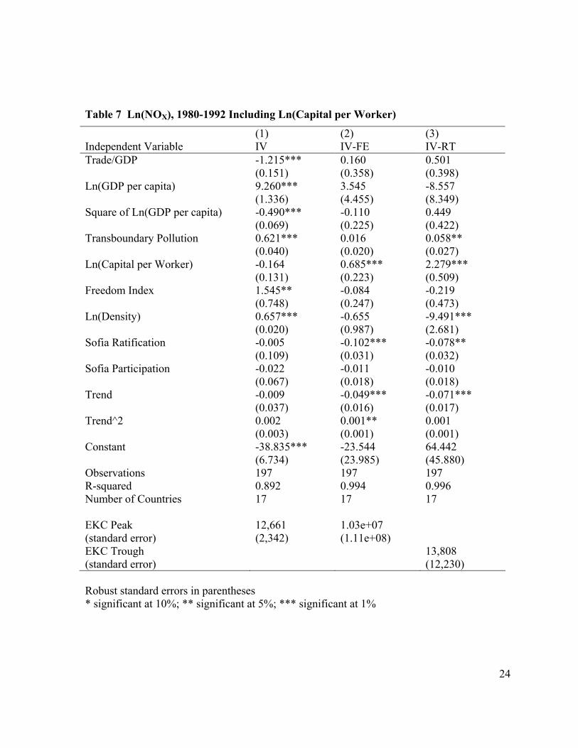
may not be appropriate either.4 Figure 1 plots sulfur dioxide (SO2) emissions against mean

SO2 concentrations in 1995 for twenty eight countries. The correlation between these two

variables is only 0.048, suggesting that air quality data may not be an appropriate proxy for

emissions. In Figure 2 nitrogen oxides’ (NOX) emissions are plotted against nitrogen dioxide

(NO2) concentrations for twenty six countries in 1995. Again, there is only a 0.098

correlation between emissions and air quality. While controlling for monitoring-site specific

characteristics alleviates some of the problems with air quality data, emissions data will

provide a better test of the existing theories.

Nitrogen oxides and sulfur dioxide are both production byproducts that pollute the

air. Once in the air, these pollutants may travel great distances resulting in acid rain and

worsened air quality not only in the country of origin but in other countries as well. Because

3 Antweiler, Copeland and Taylor (2001), Harbaugh, Levinson, and Wilson (2002), and Frankel and Rose (2005) use the Global Environment Monitoring System (GEMS) air quality data. GEMS data are monitoring-station level data collected from over forty countries. Dean (2002) examines the effect of trade on Chinese water pollution. 4 For example, the average standard deviation in SO2 concentrations is 57 percent of the mean SO2 concentrations for the sixteen countries that report concentrations for more than one monitoring station. That for NOX concentration levels is 32 percent for the twelve countries with more than one reporting monitoring stations. The 1995 data used in this footnote are reported by World Bank’s 1998 World Development Index available online at http://www.worldbank.int/nipr/wdi98/index.htm.

3

of the transboundary feature to these pollutants, three international environmental agreements

are in effect to control their emissions. The 1985 Helsinki Protocol required ratified nations

to reduce their sulfur emissions by 30 percent from 1980 emissions levels by 1990. The

1994 Oslo Protocol further restricts sulfur emissions, while the 1988 Sofia Protocol deals

with reductions of nitrogen oxides. These agreements are written and signed at international

meetings, but nations are not bound by an agreement until they ratify it. Figure 3 presents

the SO2 and NOX emissions by country for 1980-2000. Fifteen of the nineteen countries in

the sample reduced their SO2 emissions during the sample period, with average reductions of

78 percent. Twelve countries reduced their NOX emissions, with average reductions of 31

percent.5

In the long run a ten percentage point increase in openness to trade (trade/GDP)

reduces SO2 and NOX emissions by more than ten percent. Second, the environmental

Kuznets curve derived from cross-sectional variation has the expected inverse-U shape and

peaks at about $9,000. Third, a one percent increase in transboundary pollution increases

SO2 and NOX emissions by approximately half a percent. All these are both economically

and statistically significant results, robust across specifications without country fixed effects.

Introduction of fixed effects results in estimates that are calculated based on time

series variation and represent shorter-term effects. In general, no firm conclusions can be

drawn from the fixed effects models. This may be driven by insufficient variation in

variables across this time period for the sample of countries. Finally, I estimate random trend 5 Ringquist and Kostadinova (2005) use the data from 1980-1994 and find that the Helsinki Protocol was not effective in cutting emissions. Longer time series used in my study may provide new evidence. Murdoch, Sandler, and Sargent (1997) find that the Helsinki Protocol was effective in reducing sulfur, while the Sofia protocol did not have a significant effect on nitrogen oxides emissions.

4

models that allow country-specific trends in emissions. In the random trend models only

capital per worker has a significant and robust coefficient. A one percent increase in capital

per worker increases SO2 emissions by more than one percent and NOX emissions by more

than two percent.

II. Previous Literature This paper is related to three existing studies that explicitly examine the effect of

trade on the environment.6 Each uses international air quality data. Antweiler, Copeland,

and Taylor (2001) estimate the scale, composition and technique effects of trade on the

environment. The negative scale effect of trade on the environment arises because trade

tends to increase GDP, which in turn increases industrial production and emissions. The

composition effect accounts for the changes in environmental quality due to changes in the

composition of national output (shifts of production from clean to dirty or from dirty to clean

industries), and it may increase or decrease environmental quality depending on the country’s

comparative advantage. The authors find the composition effects to be small and negative.

The positive technique effect is due to increased income which results in higher demand for

cleaner production techniques. The overall effect of trade on the environment is found to be

positive, so the positive technique effect outweighs the negative scale and composition

effects. These separate effects are estimated using interacted variables.7

6 Dean (2002) estimated trade’s impact on water pollution in China. 7 Antweiler, Copeland, and Taylor (2001) specify the partial effect of openness to trade on pollution as

2 20 1 2 3 4 5( / ) ( / ) ( / )K L K L Inc Inc K L IncΨ = Ψ + Ψ + Ψ + Ψ + Ψ + Ψ , where K/L is capital per

worker and Inc is per capita income.

5

Harbaugh, Levinson, and Wilson (2002) include openness to trade without any of the

interaction terms of Antweiler, Copeland, and Taylor (2001) and find a positive effect of

trade on the environment. Both of these studies use Global Environmental Monitoring

System data that reports air quality in cities from over forty countries. While these studies do

control for some of the city characteristics, openness to trade is measured at the country

level.

Frankel and Rose (2005) correct for the simultaneity problem present in preceding

studies by instrumenting for income, income squared and openness to trade. There is a two-

way link between each of the three variables. Trade impacts the environment through the

scale, composition and technique effects described in the beginning of this section. The net

effect may be positive or negative. However, environmental regulation may also affect trade

flows across countries—the basis for the pollution haven hypothesis which states that

countries with lower environmental regulations export dirty goods.

The effect of income on environmental quality can be presented as the environmental

Kuznets curve—the inverse-U shaped relationship implying that an increase in income

increases emissions in poor countries and reduces it in rich countries. Environmental

regulation may also impact income through productivity—either by dampening or

stimulating it. Finally, the gains-from-trade hypothesis implies a positive effect of trade on

income while the gravity models of trade find that higher income can also cause more trade.

After allowing for all these possibilities in their empirical specification, Frankel and Rose

(2005) still find a positive impact of trade on air quality. Air quality in their study is

measured as the country’s average concentration of NO2, SO2 and suspended particulate

6

matter across monitoring stations. As discussed above, the correlation between such an

average and actual emissions is low and hence may not provide a good test of the

environmental impact of trade.

III. Empirical Model Pollution emissions are estimated as a function of trade, income, and other country-

specific factors:

20 1 2 3

4

( / ) ( ) [ ( )], 1,...,

it it it it

it it

E Trade GDP Ln Inc Ln IncX i n

β β β ββ ε

= + + + + + =

, (1)

where Eit is the log of either SO2 or NOX emissions in country i at time t, Trade/GDP is

openness to trade measured by imports plus exports over GDP and Inc is GDP per capita.

While previous empirical evidence finds that openness to trade tends to improve air quality,

this impact may or may not hold for emissions. Aggregated measures of air quality across

cities are not really correlated with aggregate emissions. Therefore, it is possible that the

results using this dataset provide new and different insight. To allow for the inverse-U

shaped environmental Kuznets curve (EKC), I include the log of income and the square of

log of income. The EKC hypothesis would be supported if the linear term of income has a

positive coefficient and the quadratic term has a negative coefficient. I instrument for

openness to trade, income and income squared because of the potential simultaneity problem.

The matrix X includes transboundary pollution, freedom index, population density,

capital per worker, and treaty ratification and participation variables. The transboundary

pollution variable is calculated as the weighted sum of other countries’ pollution transported

7

across borders to country i, n

ji jtj i

Eω≠

∑ i . The weight, jiω , is the percent of country j’s

emissions, Ejt, that end up in country i. These weights are calculated using atmospheric

chemistry models of source and receptor relationships and are time invariant. While the

emissions of different countries may be changing over time, the geo-spatial factors

contributing to transboundary pollution have likely not changed much over the last couple of

decades. Using Ejt in estimation of Eit and Eit in the estimation of Ejt introduces an

endogeneity problem. Therefore, I instrument for transboundary pollution using the standard

instruments for this type of problem, the weighted sums of other exogenous variables. The

weights used in construction of instruments are the same, jiω -s, described above. A similar

approach was used by Murdoch, et al. (1997) and Murdoch et al. (2003) to determine the

effect of transboundary pollution on emission-reductions and treaty participation.

A positive coefficient on transboundary pollution may be driven by coordination in

environmental regulation across countries. Such behavior could be explained by competition

in environmental taxes to attract FDI. Davies and Naughton (2006) develop one such model

and find that the slope of the best response function of environmental taxes across countries

is positive. Note that if countries’ environmental regulations tend to move in the same

direction, then emissions should also move in the same direction.

On the other hand, a negative coefficient could be indicative of a best response

function with a negative slope. For an example of such interactions imagine that winds

always blow from West to East and much of France’s pollution is transferred to Germany but

none of Germany’s pollution crosses over to France. Then if France increases its emissions

8

taxes, Germany would reduce its emissions taxes to encourage reductions in transboundary

pollution and encourage FDI.

To control for differences in environmental regulations across countries I construct a

freedom index from the civil liberties and political rights indices provided by Freedom

House. This index proxies for people’s ability to assert their preferences about

environmental policy. Civil liberties and political rights take on values between one and

seven, where lower numbers are associated with higher civil liberties and political rights.

The freedom index I use is the sum of the two divided by fourteen.8 The expected coefficient

on the freedom index is positive—lower civil liberties and political rights are expected to be

associated with higher emissions.

Another standard control included in the model is the log of population density.

More densely populated countries have higher energy and production needs and hence are

expected to have higher emissions. Capital per worker is available for only a sub sample of

years and thus is not included in all specifications. Because it is the capital-intensive

industries that tend to also pollute more, I expect that capital per worker increases emissions.

This empirical specification does not allow explicit estimation of the scale,

composition and technique effects of trade on emissions. Antweiler, Copeland, and Taylor

(2001) estimate these effects by including five interaction variables in addition to the

openness variable. 9 I use a log-specification that accounts for such interactions without

8 The correlation between the civil liberties and political rights indices is very high (0.8). Combining the two into one index allows for both to impact emissions without introducing multicollinearity problems. 9 See footnote 7.

9

explicitly estimating them. Including the interaction variables would reintroduce the

simultaneity problem that I am trying to control for.

I include Helsinki and Oslo Protocol ratification and participation effects in SO2

equations and the Sofia Protocol effects in the NOX equation. Protocol ratification effects are

introduced as dummy variables to capture the potential intercept shift caused by ratifying the

protocol. Protocol participation is captured through a variable indicating the number of years

since ratification to determine the protocol’s effects on emissions trends. Because countries

that ratified these protocols may have already been on a path to reduce emission faster than

the non-ratifying countries, the random trend model (allowing for country-specific trends) is

most appropriate for determining the effectiveness of protocols. The expected signs for all

treaty effects are negative.

Construction of Instruments There is simultaneity between openness to trade, income and emissions, as discussed

above. Therefore, following Frankel and Rose’s (2005) methodology I construct

instruments for the trade and income variables in that order. First, I estimate equation (2) of

bilateral trade using the gravity model of trade.

0 1 2 3 4

5 6 7 8

( / ) ( ) ( ) ( ) ( )

( * )ijt it ij jt it jt

ij ij i j ij t ijt

Ln Trade GDP Ln Dist Ln GDP Ln Pop Ln Pop

Lang Border Ln Area Area Landlocked

α α α α α

α α α α ν ε

= + + + +

+ + + + + + (2)

Log of trade as a share of GDP from country i to country j is estimated as a function of log of

distance between the two countries, log of country j’s GDP, log of country i’s population, log

of country j’s population, dummies for common language and land border, log of product of

the two countries’ areas, and a variable indicating whether neither country, one country or

10

both countries are landlocked. Equation (2) is a modified version of Frankel and Rose’s

(2005) specification—I have added for country j’s GDP and country i’s population. The

equation is estimated for 1980-2000 with year fixed effects. Each trade flow is only included

once in the estimation equation. That is, if /ijt itTrade GDP is included in the estimation, then

/jit jtTrade GDP is excluded from the analysis.

When constructing the instrument each observation is used twice—once for

estimation of total trade flows of each country. The instrument for openness in country i is

constructed by taking the exponent of the estimated log of trade flows to each country j and

summing over all j countries as presented in equation (3).

( / ) exp ( / )EstimatedEstimated

ijt ititj i

Trade GDP Ln Trade GDP

≠

= ∑ (3)

The second step involves constructing an instrument for income and income squared.

Because there is a potentially endogenous relationship between trade and income, I use the

instrument for openness constructed above in instrumental variable estimation used in this

step. Income is estimated as a function of openness to trade, log of population, log of income

lagged twenty years, investment rate, population growth rate, and education. This equation is

also estimated for 1980-2000 and includes year fixed effects.

1 2 3 , 20

4 5 6

( ) ( / ) ( ) ( )( )

Estimated

it it it i t

i it it t it

Ln Inc Trade GDP Ln Pop Ln IncInv PopGR Ln Educ

δ δ δ

δ δ δ γ ε−= + + +

+ + + + (4)

See Frankel and Rose (2002) for a discussion of equations (2) and (4). The

estimation results for equation (2) are presented in Appendix A Table A 1 with the

11

descriptive statistics of the data in Table A 2. The results for equation (4) are in Table A 3

with the descriptive statistics in Table A 4. These results support the results in Frankel and

Rose (2005) with the two added variables’ coefficients having the expected signs. Countries

with higher GDP’s tend to attract more trade, and countries with higher population (holding

GDP constant) tend to trade less. Data sources for these equations are also described in

Appendix A.

IV. Data The emissions data come from the Co-operative Programme for Monitoring and

Evaluation of the Long Range Transmission of Air Pollutants in Europe (EMEP, 2005) and

are country level sulfur dioxide (SO2) and nitrogen oxides (NOX) emissions for nineteen

European countries for 1980-2000 measured in gigagrams. The transboundary pollution

variable is constructed using emissions transport matrices for SO2 and NOX, and is reported

by the Meteorological Synthesizing Centre—West (MSC-W, 2002). Appendix B reports the

actual weighting matrices used in the analysis.10

Trade as a fraction of GDP, GDP per capita and population density come from 2004

World Development Indicators compiled by World Bank. Capital per worker is reported by

Penn World Tables 5.6 for 1980-1992. Note that all money values used in this analysis are in

1995 US dollars. The civil liberties and political rights indices that I use in construction of

my freedom index are reported by Freedom House online at

http://www.freedomhouse.org/ratings/index.htm.

10 Each row in the matrix answers the following question: where do the pollutants in a given country come from? The first row in Table B 1, for example, implies that 0.68% of Belgium’s, 0.84% of France’s, and 2.57% of Germany’s SO2 emissions end up in Austria.

12

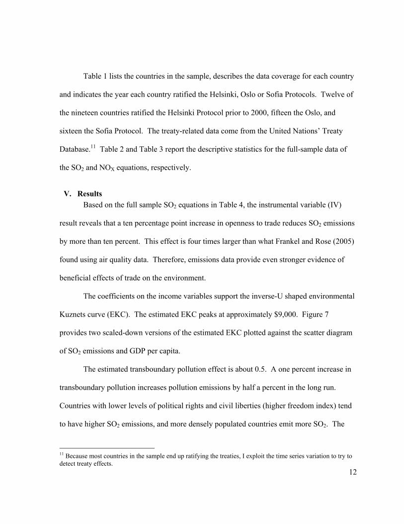
Table 1 lists the countries in the sample, describes the data coverage for each country

and indicates the year each country ratified the Helsinki, Oslo or Sofia Protocols. Twelve of

the nineteen countries ratified the Helsinki Protocol prior to 2000, fifteen the Oslo, and

sixteen the Sofia Protocol. The treaty-related data come from the United Nations’ Treaty

Database.11 Table 2 and Table 3 report the descriptive statistics for the full-sample data of

the SO2 and NOX equations, respectively.

V. Results Based on the full sample SO2 equations in Table 4, the instrumental variable (IV)

result reveals that a ten percentage point increase in openness to trade reduces SO2 emissions

by more than ten percent. This effect is four times larger than what Frankel and Rose (2005)

found using air quality data. Therefore, emissions data provide even stronger evidence of

beneficial effects of trade on the environment.

The coefficients on the income variables support the inverse-U shaped environmental

Kuznets curve (EKC). The estimated EKC peaks at approximately $9,000. Figure 7

provides two scaled-down versions of the estimated EKC plotted against the scatter diagram

of SO2 emissions and GDP per capita.

The estimated transboundary pollution effect is about 0.5. A one percent increase in

transboundary pollution increases pollution emissions by half a percent in the long run.

Countries with lower levels of political rights and civil liberties (higher freedom index) tend

to have higher SO2 emissions, and more densely populated countries emit more SO2. The

11 Because most countries in the sample end up ratifying the treaties, I exploit the time series variation to try to detect treaty effects.

13

Helsinki Protocol participation effect is negative and statistically significant. No other treaty

variable is statistically significant in the IV specification.

Fixed Effects and Random trend models To better capture the treaty effects on emissions I next control for country fixed

effects (IV-FE). The results here are driven by time series variation and present shorter-term

impacts than those estimated without fixed effects. As noted earlier, openness to trade does

not change much over time for most countries in the sample. That is likely why the

coefficient on openness to trade becomes insignificant.

The estimated EKC no longer peaks within the data as it did in the IV specification.

Transboundary pollution effect, which is likely to vary little across time, became

insignificant as well. The coefficient on the Freedom index, which is virtually constant for

eleven of the nineteen countries as shown in Figure 5, flips signs. Countries that improved

their civil liberties and political rights during 1980-2000 also tended to increase their

emissions. The coefficient on log of density, which now controls for population growth

(because the constant area effect is washed out by the country fixed effects), is still positive

and significant.

Introduction of fixed effects has changed the statistical significance for all four treaty

effects. Helsinki participation which was previously significant became insignificant, while

the other three are significant in the IV-FE specification.

If treaty participants were cutting their emissions faster even before joining the treaty

then a statistically significant treaty effect in the fixed effects model may be driven by this

trend and not by an explicit treaty effect. To control for that possibility, I add country-

14

specific trends to the IV-FE model. These random trend models (IV-RT) allow for the

possibility that the countries may have been on a path to reduce their emissions at a certain

rate over time and the environmental treaties affect emissions beyond the preexisting trends

in emissions.

In the random trend model, Helsinki Protocol participation variable is actually

positive and significant, implying that participation in the Helsinki Protocol may have

hindered the reductions in emissions. The Oslo Protocol participation effect still comes

through negative and significant. In the random trend model, openness to trade becomes

statistically significant again and is smaller in magnitude. Finally, the coefficient on the log

of density implies that population growth tended to lower emissions after controlling for the

country-specific trends.

Capital per Worker Theoretical literature suggests that trade’s impact on the environment is in part

determined by the country’s comparative advantage in the production of clean and dirty

goods. To control for the comparative advantage, in Table 5, I include capital per worker to

the estimation equation. The sample now spans from 1980-1992 (instead of 1980-2000) and

Germany and Hungary are dropped from the analysis because of unavailability of data. With

that, several observations should be made.

First, in the IV specification the coefficient on the openness to trade increases in

absolute value (from -1.19 to -1.46). This, as found in unreported results, was caused by

shortened time series. Second, the coefficient on the Freedom Index almost triples in size.

The cause of this was exclusion of Germany and Hungary from the sample. Exclusion of

15

these two countries is the main cause for the change in the estimated EKC peak from $9,000

to $11,700. Third, log of capital per worker is significant only once I control for country-

specific trends. Figure 6 presents capital per worker by country for 1980-1992. Given the

strong upward trends in capital per worker in almost all the countries, it is reasonable that

this variable becomes significant only after de-trending the data. A one percent increase in

capital per work increases SO2 emissions by more than one percent.

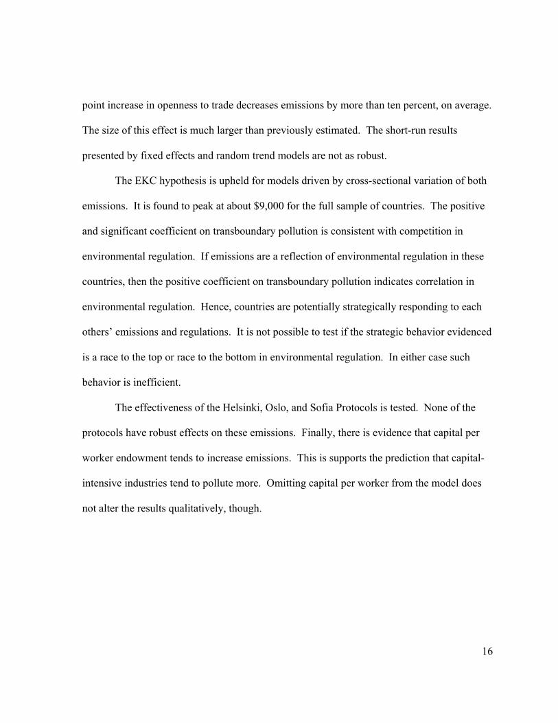
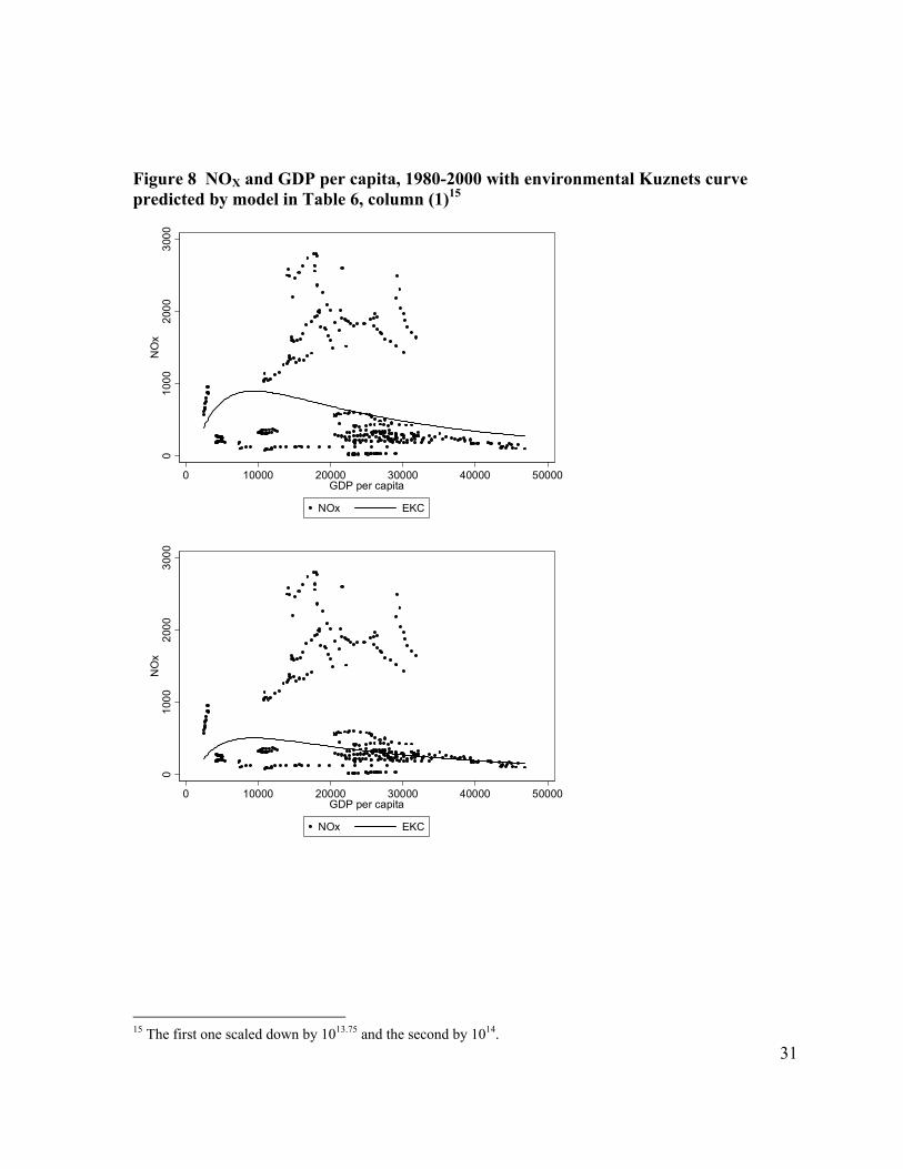
NOX Emissions To test the robustness of my results, I also estimate these equations for NOX

emissions. Because the correlation between SO2 and NOX emissions is very high (0.86) I do

not expect the results to change significantly. Table 6 provides the results for the long time

series, 1980-2000, where the openness to trade coefficient is slightly larger in absolute value,

statistically significant in the fixed effects model but not statistically significant in the

random trend model. The other noteworthy change in the results occurs with the addition of

log of capital per worker to the model. In Table 7, the elasticity of capital per worker is

statistically significant in the fixed effects model and double the size in the random trend

model. Thus, capital per worker seems to have a larger impact on NOX emissions than on

SO2 emissions.

VI. Conclusion This study adds to the current literature by estimating trade’s impact on emissions

instead of air quality. Correlations between country-average measures of air quality and

emissions are very low, and this change in the data has significant effects on the results. I

find that in the long run openness to trade reduces SO2 and NOX emissions. A ten percentage

16

point increase in openness to trade decreases emissions by more than ten percent, on average.

The size of this effect is much larger than previously estimated. The short-run results

presented by fixed effects and random trend models are not as robust.

The EKC hypothesis is upheld for models driven by cross-sectional variation of both

emissions. It is found to peak at about $9,000 for the full sample of countries. The positive

and significant coefficient on transboundary pollution is consistent with competition in

environmental regulation. If emissions are a reflection of environmental regulation in these

countries, then the positive coefficient on transboundary pollution indicates correlation in

environmental regulation. Hence, countries are potentially strategically responding to each

others’ emissions and regulations. It is not possible to test if the strategic behavior evidenced

is a race to the top or race to the bottom in environmental regulation. In either case such

behavior is inefficient.

The effectiveness of the Helsinki, Oslo, and Sofia Protocols is tested. None of the

protocols have robust effects on these emissions. Finally, there is evidence that capital per

worker endowment tends to increase emissions. This is supports the prediction that capital-

intensive industries tend to pollute more. Omitting capital per worker from the model does

not alter the results qualitatively, though.

17

References

Antweiler, Werner, Brian R. Copeland, and M. Scott Taylor. (2001) “Is Free Trade Good for

the Environment?” The American Economic Review, 91(4), 877-908.

Birdsall, N., and David Wheeler. (1993) “Trade Policy and Industrial Pollution in Latin

America: Where are the Pollution Havens?” Journal of Environment and

Development, 2(1), 137-149.

Brunnermeier, Smita B., and Arik Levinson. (2004) “Examining the Evidence on

Environmental Regulations and Industry Location,” Journal of Environment and

Development, 13(1), 6-41.

Dean, Judith M. (2002) “Does Trade Liberalization Harm the Environment? A New Test,”

Canadian Journal of Economics, 35(4), 819-842.

EMEP. (2005) “Transboundary Acidification, Eutrophication and Ground Level Ozone in

Europe in 2003,” EMEP Status Report 2005, July 20, 2005.

Feenstra, Robert C., Robert E. Lipsey, Haiyan Deng, Alyson C. Ma, and Hengyong Mo.

(2005) “World Trade Flows: 1962-2000,” NBER Working Paper 11040.

Frankel, Jeffrey A., and Andrew K. Rose. (2002) “An Estimate of the Effect of Common

Currencies on Trade and Income,” The Quarterly Journal of Economics, May 2002.

Frankel, Jeffrey A., and Andrew K. Rose. (2005) “Is Trade Good or Bad for the

Environment? Sorting Out the Causality,” The Review of Economics and Statistics,

87(1), 85-91.

18

Harbaugh, William T., Arik Levinson, and David M. Wilson. (2002) “Reexamining the

Empirical Evidence for an Environmental Kuznets Curve,” The Review of Economics

and Statistics, 84(3), 541-551.

Lucas, Robert E.B., David Wheeler, and Hemamala Hettige. (1992) “Economic

Development, Environmental Regulation and the International Migration of Toxic

International Pollution: 1960-1988,” in Patrick Low’s International Trade and the

Environment (World Bank Working Paper #1718). Washington, DC: World Bank.

Murdoch, James C., Todd Sandler, and Keith Sargent. (1997) “A Tale of Two Collectives:

Sulfur versus Nitrogen Oxides Emission Reduction in Europe,” Economica, 64, 281-

301.

Murdoch, James C., Todd Sandler, and Wim P.M. Vijverberg. (2003) “The Participation

Decisions Versus the Level of Participation in an Environmental Treaty: A Spatial

Probit Analysis,” Journal of Public Economics, 87, 337-362.

MSC-W. (2002) “Emission Data Reported to UNECE/EMEP: Quality Assurance and Trend

Analysis & Presentation of WebDab,” MSC-W Status Report 2002, July 2002.

Naughton, Helen T. (2006) “Cooperation in Environmental Policy: A Spatial Approach,”

Working Paper.

Ringquist, Evan J., and Tatiana Kostadinova. (2005) “Assessing the Effectiveness of

International Environmental Agreements: The Case of the 1985 Helsinki Protocol,”

American Journal of Political Science, 49(1), 86-102.

19

Table 1 List of Countries

Country Obs in Ln(SO2)

Obs in Ln(NOX)

Helsinki Protocol

Oslo Protocol

Sofia Protocol

1 Austria 21 21 1987 1998 1990 2 Belgiuma 20 16 1989 2000 2000 3 Denmark 21 21 1986 1997 1993 4 Finland 21 21 1986 1998 1990 5 France 21 21 1986 1997 1989 6 Germanyb,c,d 9 9 1987 1998 1990 7 Greecea 12 13 -- 1998 1998 8 Hungaryd 21 21 1986 -- 1991 9 Icelanda 19 19 -- -- -- 10 Ireland 21 21 -- 1998 1994 11 Italya 20 20 1990 1998 1992 12 Netherlands 21 21 1986 1995 1989 13 Norway 21 21 1986 1995 1989 14 Portugala 15 15 -- -- -- 15 Spain 21 21 -- 1997 1990 16 Sweden 21 21 1986 1995 1990 17 Switzerland 21 21 1987 1998 1990 18 Turkeye 13 13 -- -- -- 19 United Kingdom 21 21 -- 1996 1990 Bulgaria is dropped from the analysis since data is only available for 2000. Including this observation in the analysis does not alter the results. a The omitted observations are due to missing emissions data. b Data for 2000 are omitted due to missing emissions data. c Data for Germany between 1980-1990 are omitted because the emissions are only available for Germany as a whole. d Germany and Hungary are dropped from the analysis with the inclusion of capital per worker variable in the regression. e Data from 1980-1988 for Turkey is omitted because GDP per capita before 1968 is missing (these data would be used as lagged GDP per capita in construction of instrument for income).

20

Table 2 Descriptive Statistics for the Full Sample Ln(SO2) Equations

Variable Obs Mean Std. Dev. Min Max Ln(SO2) 360 5.758 1.474 2.785 8.489 SO2 360 779 1,002 16 4,859 Trade/GDP 360 0.717 0.286 0.305 1.824 Ln(GDP per capita) 360 9.844 0.646 7.787 10.754 GDP per capita 360 22,036 10,064 2,410 46,816 Square of Ln(GDP per capita)

360 97.315 12.138 60.644 115.648

Transboundary Pollution 360 1.008 0.998 0.028 5.022 Ln(Capital per Worker) 200 10.561 0.650 8.471 11.966 Freedom Index 360 0.201 0.124 0.143 0.786 Ln(Density) 360 4.337 1.244 0.822 6.152 Helsinki Ratification 360 0.453 0.498 0 1 Oslo Ratification 360 0.147 0.355 0 1 Helsinki Participation 360 3.025 4.338 0 14 Oslo Participation 360 0.244 0.815 0 5 Trend 360 11.258 5.933 1 21 Trend2 360 162 134 1 441

Table 3 Descriptive Statistics for the Full Sample Ln(NOX) Equations

Variable Obs Mean Std. Dev. Min Max Ln(NOX) 357 5.924 1.139 3.020 7.934 NOX 357 670 725 21 2,791 Trade/GDP 357 0.709 0.279 0.305 1.824 Ln(GDP per capita) 357 9.841 0.649 7.787 10.754 GDP per capita 357 22,009 10,126 2,410 46,816 Square of Ln(GDP per capita)

357 97.26 12.20 60.64 115.65

Transboundary Pollution 357 1.260 1.187 0.097 5.445 Ln(Capital per Worker) 197 10.554 0.654 8.471 11.966 Freedom Index 357 0.202 0.125 0.143 0.786 Ln(Density) 357 4.322 1.241 0.822 6.152 Sofia Ratification 357 0.409 0.492 0 1 Sofia Participation 357 1.950 3.096 0 11 Trend 357 11.359 5.878 1 21 Trend2 357 163.465 133.300 1 441

21

Table 4 Ln(SO2), 1980-2000

(1) (2) (3) Independent Variable IV IV-FE IV-RT Trade/GDP -1.190*** -1.146 -0.573** (0.130) (1.023) (0.282) Ln(GDP per capita) 20.211*** 32.103*** -0.536 (1.324) (10.669) (7.869) Square of Ln(GDP per capita) -1.110*** -1.466*** 0.094 (0.068) (0.499) (0.399) Transboundary Pollution 0.514*** -0.024 -0.060 (0.032) (0.112) (0.053) Freedom Index 2.263*** -1.660*** 0.444 (0.435) (0.478) (0.309) Ln(Density) 0.612*** 5.853*** -6.247*** (0.021) (1.260) (1.591) Helsinki Ratification -0.054 -0.186*** -0.021 (0.112) (0.069) (0.043) Oslo Ratification -0.190 -0.204*** -0.030 (0.145) (0.070) (0.039) Helsinki Participation -0.058*** -0.004 0.052*** (0.017) (0.025) (0.013) Oslo Participation 0.009 -0.073** -0.037 (0.046) (0.033) (0.025) Trend -0.081*** -0.174*** -0.152*** (0.029) (0.045) (0.016) Trend^2 0.005*** 0.003* -0.000 (0.001) (0.001) (0.001) Constant -87.596*** -193.968*** 30.539 (6.502) (57.620) (42.790) Observations 360 360 360 R-squared 0.862 0.971 0.993 Number of Countries 19 19 19 EKC Peak 9,028 56,830 (514) (14,114) EKC Trough 17 (463) Robust standard errors in parentheses * significant at 10%; ** significant at 5%; *** significant at 1%

22

Table 5 Ln(SO2), 1980-1992 Including Ln(Capital per Worker)

(1) (2) (3) Independent Variable IV IV-FE IV-RT Trade/GDP -1.459*** 1.101 0.206 (0.198) (0.741) (0.461) Ln(GDP per capita) 22.417*** 14.409 -22.795 (1.712) (12.179) (17.671) Square of Ln(GDP per capita) -1.196*** -0.597 1.265 (0.091) (0.644) (0.886) Transboundary Pollution 0.536*** -0.035 -0.004 (0.051) (0.093) (0.061) Ln(Capital per Worker) -0.010 -0.206 1.131** (0.178) (0.385) (0.453) Freedom Index 6.244*** 0.183 0.138 (0.967) (0.484) (0.593) Ln(Density) 0.678*** 9.297*** -4.332 (0.029) (2.219) (4.211) Helsinki Ratification -0.253* -0.055 -0.020 (0.133) (0.072) (0.044) Helsinki Participation -0.117*** -0.098*** -0.021 (0.042) (0.024) (0.022) Trend -0.056 -0.194*** -0.256*** (0.049) (0.031) (0.024) Trend^2 0.006 0.006*** 0.002 (0.004) (0.002) (0.001) Constant -101.656*** -119.074* 115.185 (8.535) (62.570) (102.385) Observations 200 200 200 R-squared 0.872 0.987 0.996 Number of Countries 17 17 17 EKC Peak 11,719 173,444 (1,156) (337,684) EKC Trough 8,206 (5,230) Robust standard errors in parentheses * significant at 10%; ** significant at 5%; *** significant at 1%

23

Table 6 Ln(NOX), 1980-2000

(1) (2) (3) Independent Variable IV IV-FE IV-RT Trade/GDP -1.368*** -1.215*** -0.107 (0.128) (0.466) (0.216) Ln(GDP per capita) 8.717*** 16.954*** 2.886 (1.288) (4.127) (3.674) Square of Ln(GDP per capita) -0.477*** -0.727*** -0.126 (0.066) (0.192) (0.179) Transboundary Pollution 0.455*** 0.015 0.020 (0.036) (0.037) (0.020) Freedom Index 0.046 -0.880*** 0.274 (0.363) (0.304) (0.191) Ln(Density) 0.592*** 1.225* -4.219*** (0.016) (0.664) (1.330) Sofia Ratification -0.114 -0.042 -0.013 (0.089) (0.035) (0.026) Sofia Participation -0.004 -0.018* -0.026* (0.019) (0.009) (0.015) Trend -0.034 -0.067*** 0.009 (0.021) (0.021) (0.012) Trend^2 0.002** 0.001** 0.000 (0.001) (0.001) (0.001) Constant -35.643*** -95.844*** 8.149 (6.315) (22.220) (19.130) Observations 357 357 357 R-squared 0.838 0.985 0.995 Number of Countries 19 19 19 EKC Peak 9,363 115,390 90,284 (1,057) (38,358) (313,378) Robust standard errors in parentheses * significant at 10%; ** significant at 5%; *** significant at 1%

24

Table 7 Ln(NOX), 1980-1992 Including Ln(Capital per Worker)

(1) (2) (3) Independent Variable IV IV-FE IV-RT Trade/GDP -1.215*** 0.160 0.501 (0.151) (0.358) (0.398) Ln(GDP per capita) 9.260*** 3.545 -8.557 (1.336) (4.455) (8.349) Square of Ln(GDP per capita) -0.490*** -0.110 0.449 (0.069) (0.225) (0.422) Transboundary Pollution 0.621*** 0.016 0.058** (0.040) (0.020) (0.027) Ln(Capital per Worker) -0.164 0.685*** 2.279*** (0.131) (0.223) (0.509) Freedom Index 1.545** -0.084 -0.219 (0.748) (0.247) (0.473) Ln(Density) 0.657*** -0.655 -9.491*** (0.020) (0.987) (2.681) Sofia Ratification -0.005 -0.102*** -0.078** (0.109) (0.031) (0.032) Sofia Participation -0.022 -0.011 -0.010 (0.067) (0.018) (0.018) Trend -0.009 -0.049*** -0.071*** (0.037) (0.016) (0.017) Trend^2 0.002 0.001** 0.001 (0.003) (0.001) (0.001) Constant -38.835*** -23.544 64.442 (6.734) (23.985) (45.880) Observations 197 197 197 R-squared 0.892 0.994 0.996 Number of Countries 17 17 17 EKC Peak 12,661 1.03e+07 (standard error) (2,342) (1.11e+08) EKC Trough 13,808 (standard error) (12,230) Robust standard errors in parentheses * significant at 10%; ** significant at 5%; *** significant at 1%

25

Figure 1 SO2 Emissions and Mean SO2 Concentrations, 199512 0

5010

015

020

0M

ean

SO

2 C

once

ntra

tions

(mic

rogr

ams/

m^3

)

0 5000 10000 15000 20000SO2 Emissions (gigagrams)

Figure 2 NOX Emissions and Mean NO2 Concentrations, 1995

050

100

150

200

250

Mea

n N

O2

Con

cent

ratio

ns (m

icro

gram

s/m

^3)

0 5000 10000 15000 20000 25000NOx Emissions (gigagrams)

12 The SO2 and NO2 concentrations data are from 1998 World Development Indicators compiled by the World Bank available online at http://www.worldbank.int/nipr/wdi98/index.htm.

Figure 3 SO2 and NOX Emissions, 1980-2000 40

.75

384.

6

180.

882

8

27.5

452.

1

73.5

584

659

3249

831

3996

304

534

183.

316

33

16.2

29.6

7322

2

923

3757

91.2

602

26.2

123

9.5

9640

9

1033

3013

53.7

149

1

19.2

617

9

443.

121

04

1165

4859

1980 1985 1990 1995 2000

1980 1985 1990 1995 2000 1980 1985 1990 1995 2000 1980 1985 1990 1995 2000 1980 1985 1990 1995 2000

Austria Belgium Denmark Finland France

Germany Greece Hungary Iceland Ireland

Italy Netherlands Norway Portugal Spain

Sweden Switzerland Turkey United Kingdom

SO2 NOx

year

Graphs by country

27

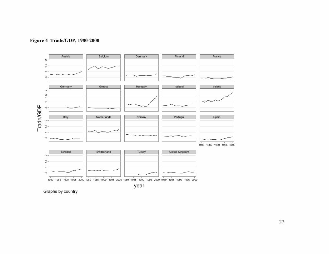
Figure 4 Trade/GDP, 1980-2000 .5

11.

52

.51

1.5

2.5

11.

52

.51

1.5

2

1980 1985 1990 1995 2000

1980 1985 1990 1995 2000 1980 1985 1990 1995 2000 1980 1985 1990 1995 2000 1980 1985 1990 1995 2000

Austria Belgium Denmark Finland France

Germany Greece Hungary Iceland Ireland

Italy Netherlands Norway Portugal Spain

Sweden Switzerland Turkey United Kingdom

Trad

e/G

DP

yearGraphs by country

28

Figure 5 Freedom Index, 1980-2000 .2

.4.6

.8.2

.4.6

.8.2

.4.6

.8.2

.4.6

.8

1980 1985 1990 1995 2000

1980 1985 1990 1995 2000 1980 1985 1990 1995 2000 1980 1985 1990 1995 2000 1980 1985 1990 1995 2000

Austria Belgium Denmark Finland France

Germany Greece Hungary Iceland Ireland

Italy Netherlands Norway Portugal Spain

Sweden Switzerland Turkey United Kingdom

Free

dom

Inde

x

yearGraphs by country

29

Figure 6 Capital per Worker, 1980-1992 39

,123

56,2

47

47,5

2659

,803

48,3

0157

,869

54,5

3177

,169

44,3

9057

,135

20,6

7524

,674

18,5

3137

,157

22,4

7328

,334

27,3

5036

,380

42,9

5650

,604

56,4

6767

,281

7,94

413

,215

21,9

8734

,956

48,0

8968

,553

116,

971

157,

297

4,77

64,

882

19,1

2825

,994

1980 1990 1980 1990 1980 1990 1980 1990 1980 1990

1980 1990 1980 1990 1980 1990 1980 1990 1980 1990

1980 1990 1980 1990 1980 1990 1980 1990 1980 1990

1980 1990 1980 1990

Austria Belgium Denmark Finland France

Greece Iceland Ireland Italy Netherlands

Norway Portugal Spain Sweden Switzerland

Turkey United Kingdom

Cap

ital p

er W

orke

r

yearGraphs by country

30

Figure 7 SO2 and GDP per capita, 1980-2000 with environmental Kuznets curve predicted by model in Table 4, column (1)14

010

0020

0030

0040

0050

00S

O2

0 10000 20000 30000 40000 50000GDP per capita

SO2 EKC

010

0020

0030

0040

0050

00S

O2

0 10000 20000 30000 40000 50000GDP per capita

SO2 SO2

14 The first graph scaled by 10^37, the second by 10^37.5.

31

Figure 8 NOX and GDP per capita, 1980-2000 with environmental Kuznets curve predicted by model in Table 6, column (1)15

010

0020

0030

00N

Ox

0 10000 20000 30000 40000 50000GDP per capita

NOx EKC

010

0020

0030

00N

Ox

0 10000 20000 30000 40000 50000GDP per capita

NOx EKC

15 The first one scaled down by 1013.75 and the second by 1014.

32

Appendix A Instrument Equations

Table A 1 Bilateral Trade Equation, 1980-2000

Independent Variable Ln(Tradeij/GDPi)Ln(Distance) -0.78*** (122.93) Ln(Country 2 GDP) 0.92*** (290.24) Ln(Country 1 Population) -0.07*** (17.10) Ln(Country 2 Population) -0.04*** (7.81) Common Language Dummy 0.77*** (53.36) Common Border Dummy 0.89*** (26.68) Ln(Product of Areas) -0.07*** (28.38) Landlocked (0, 1, or 2) -0.45*** (40.96) Constant -20.16*** (211.59) Observations 72,344 R-squared 0.73 Robust t statistics in parentheses, includes year dummy variables * significant at 10%; ** significant at 5%; *** significant at 1%

Table A 2 Descriptive Statistics for Bilateral Trade Equation

Variable Obs Mean Std. Dev. Min Max Ln(Trade/GDP) 76,945 -7.303 2.579 -18.745 1.237 Ln(Distance) 76,945 8.611 0.827 4.088 9.892 Ln(Country 2 Population) 76,945 9.521 1.620 4.025 14.049 Common Language Dummy 76,945 0.156 0.363 0 1 Common Border Dummy 76,945 0.027 0.163 0 1 Ln(Product of Areas) 76,945 24.543 3.077 7.189 32.769 Landlocked (0, 1, or 2) 76,945 0.220 0.445 0 2

33

Table A 3 Income Equation, 1980-2000

Independent Variable Ln(GDP per capita)Trade/GDP 0.24*** (5.56) Ln(Population) 0.07*** (8.38) Ln(GDP per capita Lagged 20 years) 0.85*** (71.70) Average Investment/GDP 0.02*** (8.94) Population Growth Rate -0.16*** (14.45) Ln(Average Years of Schooling) 0.22*** (13.37) Constant 0.02 (0.12) Observations 1708 R-squared 0.97 Robust t statistics in parentheses, includes year dummy variables * significant at 10%; ** significant at 5%; *** significant at 1%

Table A 4 Descriptive Statistics for Income Equation

Variable Obs Mean Std. Dev. Min Max Ln(GDP per capita) 1,708 7.918 1.613 4.805 10.754 Trade/GDP 1,708 0.664 0.399 0.063 2.960 Constructed Trade/GDP 1,708 0.204 0.170 0.025 1.348 Ln(Population) 1,708 16.286 1.597 12.337 20.956 Ln(GDP per capita Lagged 20 years)

1,708 7.597 1.512 4.170 10.733

Average Investment/GDP 1,708 16.590 7.163 2.477 32.019 Population Growth Rate 1,708 1.843 1.056 -0.407 7.635 Ln(Average Years of Schooling)

1,708 1.569 0.650 -0.942 2.506

34

Data Sources for Bilateral Trade Equation Bilateral trade data are reported by Feenstra et al. (2005) online at

http://cid.econ.ucdavis.edu. To convert the trade data into constant 1995 US dollars I use the

US GDP deflator as reported by the Economic Report of the President. Data for distances

between countries, common language, common border, area and whether or not a country is

landlocked come from Centre d’Etudes Prospectives et d’Informations Internationales

(CEPII) available online at http://www.cepii.fr/anglaisgraph/bdd/distances.htm. Population

and GDP data come from 2004 World Development Index (2004 WDI) compiled by the

World Bank.

Data Sources for Income Equation Income is measured as GDP per capita and is reported by 2004 WDI, as is trade over

GDP and the population data. Investment as a share of GDP is reported by Penn World

Tables 6.1 and is averaged over all available years. Population growth rate for a given year

in a country is calculated based on the preceding twenty years. Education measured as

average years of schooling for people aged over 25 come from the Barro and Lee (1996)

dataset available online at http://www.nber.org/pub/barro.lee/ , includes year dummy

variables and is reported every five years between 1960 and 2000. I interpolate the data for

intermittent years.

Appendix B Weighting Matrices

Table B 1 SO2 Transport Matrix Austria Belgium Denmark Finland France Germany Greece Hungary Iceland Ireland Italy Netherlands Norway Portugal Spain Sweden Switzerland Turkey United

KingdomAustria 0.00% 0.68% 0.00% 0.00% 0.84% 2.57% 0.15% 1.48% 0.00% 0.16% 2.51% 0.69% 0.00% 0.23% 0.44% 0.00% 5.38% 0.04% 0.23% Belgium 0.00% 0.00% 0.00% 0.00% 2.46% 0.73% 0.00% 0.04% 0.00% 0.31% 0.07% 3.67% 0.00% 0.23% 0.39% 0.00% 0.00% 0.00% 0.73% Denmark 0.00% 1.35% 0.00% 0.29% 0.59% 1.20% 0.00% 0.13% 1.59% 0.63% 0.05% 1.83% 0.77% 0.15% 0.28% 0.36% 0.00% 0.00% 0.94% Finland 0.51% 1.01% 2.24% 0.00% 0.56% 1.13% 0.20% 1.10% 0.00% 0.31% 0.34% 1.15% 3.08% 0.15% 0.26% 6.79% 1.08% 0.07% 0.73% France 0.51% 6.09% 0.00% 0.00% 0.00% 2.47% 0.15% 0.25% 0.00% 2.52% 2.76% 3.21% 0.00% 5.81% 14.36% 0.00% 7.53% 0.00% 2.89% Germany 5.64% 18.83% 3.73% 0.00% 10.39% 0.00% 0.15% 0.97% 0.00% 1.89% 1.85% 18.81% 0.77% 1.24% 2.43% 0.71% 20.43% 0.03% 4.42% Greece 0.51% 0.11% 0.00% 0.00% 0.19% 0.17% 0.00% 0.76% 0.00% 0.00% 1.13% 0.00% 0.00% 0.08% 0.19% 0.00% 0.00% 0.57% 0.04% Hungary 4.62% 0.23% 0.00% 0.00% 0.44% 0.68% 0.45% 0.00% 0.00% 0.00% 1.45% 0.23% 0.00% 0.15% 0.26% 0.00% 1.08% 0.04% 0.12% Iceland 0.00% 0.00% 0.00% 0.00% 0.03% 0.02% 0.00% 0.00% 0.00% 0.16% 0.00% 0.00% 0.00% 0.00% 0.08% 0.00% 0.00% 0.00% 0.14% Ireland 0.00% 0.23% 0.00% 0.00% 0.16% 0.07% 0.00% 0.00% 0.00% 0.00% 0.00% 0.23% 0.00% 0.15% 0.19% 0.00% 0.00% 0.00% 1.03% Italy 2.56% 0.56% 0.00% 0.00% 2.96% 0.76% 2.06% 0.93% 0.00% 0.31% 0.00% 0.46% 0.00% 1.16% 2.17% 0.00% 5.38% 0.15% 0.28% Netherlands 0.00% 8.57% 0.00% 0.00% 1.40% 1.00% 0.00% 0.04% 0.00% 0.31% 0.07% 0.00% 0.00% 0.15% 0.31% 0.00% 0.00% 0.00% 1.28% Norway 0.00% 1.92% 5.22% 1.14% 0.94% 1.57% 0.05% 0.47% 0.00% 0.94% 0.12% 2.29% 0.00% 0.23% 0.50% 4.29% 0.00% 0.01% 2.36% Portugal 0.00% 0.00% 0.00% 0.00% 0.09% 0.00% 0.00% 0.00% 0.00% 0.00% 0.00% 0.00% 0.00% 0.00% 1.23% 0.00% 0.00% 0.00% 0.05% Spain 0.00% 0.34% 0.00% 0.00% 1.22% 0.12% 0.10% 0.08% 0.00% 0.31% 0.49% 0.23% 0.00% 17.12% 0.00% 0.00% 0.00% 0.00% 0.37% Sweden 1.54% 2.59% 16.42% 6.86% 1.47% 3.18% 0.40% 2.12% 0.79% 0.79% 0.54% 3.44% 11.54% 0.39% 0.62% 0.00% 2.15% 0.12% 1.90% Switzerland 0.51% 0.45% 0.00% 0.00% 1.43% 0.46% 0.05% 0.04% 0.00% 0.16% 1.40% 0.23% 0.00% 0.31% 0.65% 0.00% 0.00% 0.00% 0.18% Turkey 1.03% 0.23% 0.75% 0.29% 0.34% 0.37% 7.43% 1.36% 0.00% 0.16% 1.55% 0.23% 0.77% 0.15% 0.33% 0.36% 1.08% 0.00% 0.12% United Kingdom

0.00% 2.03% 0.75% 0.00% 2.18% 0.49% 0.00% 0.08% 0.00% 10.22% 0.10% 1.83% 0.00% 0.77% 1.12% 0.36% 0.00% 0.00% 0.00%

36

Table B 2 NOX Transport Matrix Austria Belgium Denmark Finland France Germany Greece Hungary Iceland Ireland Italy Netherlands Norway Portugal Spain Sweden Switzerland Turkey United

KingdomAustria 0.00% 1.01% 0.18% 0.00% 1.13% 2.60% 0.13% 1.68% 0.00% 0.29% 3.41% 1.04% 0.19% 0.27% 0.44% 0.16% 5.35% 0.05% 0.29% Belgium 0.00% 0.00% 0.18% 0.00% 1.47% 0.55% 0.00% 0.00% 0.00% 0.59% 0.10% 1.22% 0.19% 0.27% 0.44% 0.00% 0.41% 0.00% 0.89% Denmark 0.21% 1.63% 0.00% 0.16% 0.87% 1.14% 0.00% 0.19% 3.17% 0.88% 0.13% 2.00% 1.12% 0.14% 0.30% 0.79% 0.41% 0.00% 1.35% Finland 1.24% 1.76% 4.23% 0.00% 0.87% 1.96% 0.13% 1.12% 0.00% 0.88% 0.44% 2.09% 3.17% 0.14% 0.21% 9.84% 1.23% 0.05% 1.18% France 1.24% 7.04% 0.71% 0.00% 0.00% 2.99% 0.13% 0.37% 1.59% 3.83% 3.65% 4.00% 0.56% 8.33% 16.74% 0.32% 6.58% 0.00% 4.48% Germany 6.40% 17.09% 3.53% 0.16% 10.78% 0.00% 0.13% 1.12% 1.59% 2.95% 3.05% 14.25% 1.86% 1.50% 2.63% 1.11% 15.64% 0.00% 5.95% Greece 0.62% 0.13% 0.18% 0.00% 0.26% 0.29% 0.00% 0.93% 0.00% 0.00% 1.28% 0.17% 0.00% 0.14% 0.27% 0.00% 0.41% 1.17% 0.07% Hungary 3.93% 0.50% 0.18% 0.00% 0.58% 1.12% 0.38% 0.00% 0.00% 0.00% 2.03% 0.52% 0.19% 0.14% 0.30% 0.16% 1.23% 0.05% 0.19% Iceland 0.00% 0.13% 0.18% 0.00% 0.08% 0.09% 0.00% 0.00% 0.00% 0.29% 0.00% 0.17% 0.37% 0.00% 0.06% 0.16% 0.00% 0.00% 0.31% Ireland 0.00% 0.25% 0.18% 0.00% 0.24% 0.09% 0.00% 0.00% 0.00% 0.00% 0.03% 0.26% 0.19% 0.27% 0.21% 0.00% 0.00% 0.00% 1.08% Italy 4.13% 1.13% 0.35% 0.00% 3.96% 1.54% 2.18% 1.50% 0.00% 0.29% 0.00% 0.96% 0.19% 1.37% 3.28% 0.16% 7.41% 0.15% 0.39% Netherlands 0.21% 1.88% 0.18% 0.00% 1.05% 0.48% 0.00% 0.00% 0.00% 0.59% 0.10% 0.00% 0.19% 0.27% 0.35% 0.16% 0.41% 0.00% 1.47% Norway 0.83% 3.14% 6.53% 1.62% 1.57% 2.38% 0.00% 0.37% 1.59% 1.77% 0.18% 3.56% 0.00% 0.27% 0.44% 5.56% 0.82% 0.00% 3.40% Portugal 0.00% 0.13% 0.00% 0.00% 0.18% 0.02% 0.00% 0.00% 0.00% 0.00% 0.03% 0.09% 0.00% 0.00% 1.68% 0.00% 0.00% 0.00% 0.10% Spain 0.21% 0.63% 0.18% 0.00% 1.92% 0.22% 0.13% 0.00% 0.00% 0.59% 0.57% 0.43% 0.19% 21.99% 0.00% 0.00% 0.41% 0.00% 0.75% Sweden 2.48% 4.15% 11.82% 7.14% 2.36% 4.62% 0.13% 2.24% 1.59% 1.77% 0.89% 5.04% 7.64% 0.41% 0.62% 0.00% 2.47% 0.05% 3.25% Switzerland 0.41% 0.75% 0.00% 0.00% 1.55% 0.48% 0.00% 0.00% 0.00% 0.29% 1.67% 0.35% 0.00% 0.27% 0.65% 0.00% 0.00% 0.00% 0.22% Turkey 1.03% 0.38% 0.53% 0.16% 0.45% 0.62% 8.59% 1.50% 0.00% 0.00% 1.41% 0.43% 0.37% 0.14% 0.38% 0.32% 1.23% 0.00% 0.19% United Kingdom

0.21% 2.39% 1.23% 0.16% 2.47% 0.73% 0.00% 0.19% 1.59% 10.91% 0.18% 2.26% 1.49% 1.23% 1.27% 0.48% 0.41% 0.00% 0.00%