NBER WORKING PAPER SERIES

REEXAMINING THE EMPIRICAL EVIDENCE FOR AN ENVIRONMENTAL KUZNETS CURVE

William HarbaughArik LevinsonDavid Wilson

Working Paper 7711http://www.nber.org/papers/w7711

NATIONAL BUREAU OF ECONOMIC RESEARCH1050 Massachusetts Avenue

Cambridge, MA 02138May 2000

We would like to thank Jim Ziliak for helpful comments, and the National Science Foundation and RayMikesell for financial support. The views expressed herein are those of the authors and not necessarily thoseof the National Bureau of Economic Research.

© 2000 by William Harbaugh, Arik Levinson, and David Wilson. All rights reserved. Short sections of textnot to exceed two paragraphs, may be quoted without explicit permission provided that full credit, including© notice, is given to the source.

Reexamining the Empirical Evidence for an Environmental Kuznets CurveWilliam Harbaugh, Arik Levinson, and David WilsonNBER Working Paper No. 7711May 2000JEL No. Q25, O13

ABSTRACT

This paper uses an updated and revised panel data set on ambient air pollution in cities world-

wide to examine the robustness of the evidence for the existence of an inverted U-shaped

relationship between national income and pollution. We test the sensitivity of the pollution-income

relationship to functional forms, to additional covariates, and to changes in the nations, cities, and

years sampled. We find that the results are highly sensitive to these changes. We conclude that there

is little empirical support for an inverted-U-shaped relationship between several important air

pollutants and national income in these data.

William Harbaugh Arik LevinsonDepartment of Economics Department of EconomicsUniversity of Oregon Georgetown UniversityEugene, OR 97403-1285 ICC 571 and NBER Washington, DC 20057-1036 harbaugh@oregon.uoregon.edu and NBER

am16@georgetown.edu

David WilsonDepartment of Economics University of Oregon Eugene, OR 97403-1285 dwilson@darkwing.uoregon.edu

1. Introduction

Several recent and often-cited papers on the relationship between pollution and economic

growth find that many forms of air and water pollution "initially worsen but then improve as incomes rise"

(World Bank, 1992). Grossman and Krueger (1995), in particular, report that for most pollutants, this

turning point in environmental quality typically occurs at incomes below $8000 per capita. Because of its

similarity to the pattern of income inequality documented by Kuznets (1955), this inverse-U-shaped

pollution-income pattern is sometimes called an "environmental Kuznets curve."

In response to these empirical findings, a number of researchers have sought further evidence

for inverse-U-shaped pollution-income relationships (Holtz-Eakin and Selden, 1995; Selden and Song,

1994; Hilton and Levinson, 1998; Shafik, 1994). Others have proposed theoretical explanations for the

relationship between pollution and economic growth (Selden and Song, 1995; Stokey, 1998; Jaeger,

1998; Jones and Manuelli, 1995; Andreoni and Levinson, 1998; Chaudhuri and Pfaff, 1997).1 There

are essentially two key questions being asked. The first is whether or not an inverted-U-shaped

pollution-income path can be consistent with Pareto optimality. This is the subject of much of the

theoretical literature. The second key question is whether there is sufficient empirical evidence to

conclude that environmental quality does improve eventually with economic growth, for at least some

subset of pollutants. This latter question is the focus of this paper. While the existing literature appears to

demonstrate numerous circumstances in which pollution follows an inverse-U, eventually declining with

income, we argue that the evidence is less robust than it appears.

Far from being an academic curiosity, this debate is of considerable importance to national and

international environmental policy. Based on the existing research, some policy analysts have concluded

2

that developing countries will automatically become cleaner as their economies grow (Beckerman,

1992; Bartlett, 1994). Others have argued that it is natural for the poorest countries to become more

polluted as they develop. These types of conclusions depend on the apparently growing conventional

wisdom that pollution follows a deterministic inverse-U-shaped environmental Kuznets curve.

In this paper we re-examine the empirical evidence documenting inverse-U-shaped pollution-

income relationships using the air pollution data studied by the World Bank (1992) and by Grossman

and Krueger (1995), with the benefits of a retrospective data cleaning and ten additional years of data.

We analyze three common air pollutants: sulfur dioxide (SO2), smoke, and total suspended particulates

(TSP). These are the three pollutants for which the most complete data are available.2 All three are

widely considered to cause serious health and environmental problems. Two of the three, SO2 and

smoke, exhibit the most dramatic inverse-U-shaped patterns in the World Bank (1992) and in

Grossman and Krueger (1995). We also test the sensitivity of the pollution-income relationship to the

functional forms and econometric specifications used, to the inclusion of additional covariates besides

income, and to the nations, cities, and years sampled. In addition, we construct 95-percent confidence

bands around the estimated pollution-income relationships.

Our conclusion is that the evidence for an inverted-U is much less robust than previously

thought. We find that the locations of the turning points, as well as their very existence, are sensitive to

both slight variations in the data and to reasonable permutations of the econometric specification.

Merely cleaning up the data, or including newly available observations, makes the inverse-U shape

disappear. Furthermore, econometric specifications that extend the lag structure of GDP per capita as a

1 In addition, recent special issues of two journals, Environment and Development Economics in November 1997 andEcological Economics in May 1998 include papers on the environmental Kuznets curve.2 We also tested models on lead, NOx, and other sizes of suspended particulate matter. Sample sizes were small, andthe independent variables were generally insignificant.

3

dependent variable, include additional country-specific covariates, or include country-level fixed effects,

generate predicted pollution-income relationships with very different shapes.

2. Data

The data on ambient pollution levels underlying this study are collected by the Global

Environmental Monitoring System (GEMS), sponsored by the World Health Organization (WHO) and

the United Nations.3 The EPA maintains these data in its Aerometric Information Retrieval System

(AIRS). For each pollution monitoring station, the data set we obtained contains the annual mean and

maximum for each pollutant monitored, along with descriptive variables about the neighborhood and city

in which the monitor is located.

Table 1 lists some descriptive statistics for both the original data used by Grossman and

Krueger (1995), which they have graciously made available, and for the data available from AIRS as of

December 1998. The new data contain substantially more usable observations than were originally

available. For sulfur dioxide, the number of observations goes from 1352 to 2381, with 25 new cities,

and three new countries. These data add 4 new years of observations, from 1989 to 1992, and 6

additional years of older observations, from 1971 to 1976. In addition, missing observations for existing

cities have been filled in.

The new AIRS data also include revisions of some of the original observations. To determine

the extent of these revisions, we matched the observations from the original data with those in the new

data, and then compared the pollution concentration numbers. These matches were not always easy to

make. We began by matching observations between the two data sets by pollutant, city, and year. In

most cases there were several monitoring sites per city, so observations were then paired by comparing

4

the number of measurements and mean values reported. For some cities the number of observations

was consistently the same, for others it was consistently different, and for still others it was a mix.

Using our best efforts to match the old and the new observations, we found that observations

that appeared to come from the same site and year often had very different reported pollution

concentrations. We also found that 92 of 1021 observations in the original TSP data were obvious

duplications, as were 76 of the 488 in the smoke data. These have been eliminated from the new data

set. Table 2 gives summary statistics showing the extent of the revisions. For the 485 SO2 observations

that we are most certain that we have correctly matched to the original data set, the correlation between

mean sulfur dioxide levels between the new and old data is only 0.75. For TSP and smoke this

correlation is 1.0 and 0.77 respectively. The lower part of Table 2 shows summary statistics for the

ratio of the new reported observation value to the value in the old data. If the data were identical, the

mean of this ratio would be one, and the standard deviation would be zero. For SO2 the mean of this

ratio is 1.21, while the standard deviation is 1.73. In sum, since some of the early empirical work on this

topic was completed, a large number of new observations have been added, and the existing data have

been substantially revised. We should also note that the matching procedure we followed probably

produces a downward biased picture of the extent of these revisions, because we are most likely to

match the observations that have not changed.

In the analyses that follow, we examine the data on ambient concentrations of SO2, TSP, and

smoke together with a set of variables describing national income, political structure, investment, trade,

and population density, as well as control variables that account for where the monitoring station was

located. For national income we use real per capita gross domestic product, in 1985 dollars, from the

Penn World Tables (PWT) as described in Summers and Heston (1991). This is the same income

3 GEMS was initiated in the early 1970s to coordinate the worldwide collection of comparable measures of ambient air

5

measure used by most previous studies. Our measure of political structure is an index of the extent of

democratic participation in government, from the Polity III data set described in Jaggers and Gurr

(1995). This index, which ranges from 0 to 10 with 10 being most democratic, is available for every

year and country in the AIRS data. We measure trade intensity using the ratio of imports plus exports to

GDP, and we measure investment as a fraction of GDP, both from the PWT. We use population and

country area data from a variety of sources to construct annual measures of national population density.4

3. The effects of changes in the data

To demonstrate the effects of the revisions to the existing data, we need to begin with a

benchmark econometric specification. Because Grossman and Krueger's (1995) paper is in many ways

the most carefully done and widely known work, we start with their specification. They estimate

,7'

63

52

433

22

1 itiitititititititit XLLLGGGY νµβββββββ ++++++++=

where Git is per capita gross domestic product at time t for the country in which monitoring site i is

located, Lit is a three-year average of lagged per capita GDP, and Xit are country and site-specific

descriptors. This model was estimated using random effects, so mi is assumed to be a site specific effect

that is uncorrelated with the right-hand-side variables, and nit is a normally distributed error term.

Table 3 estimates this equation for SO2. Column 1 replicates the Grossman and Krueger results

exactly, using their data. The dependent variable in column 1 is the median annual sulfur dioxide reading

from each monitor. Because the version of the data we obtained from the EPA reports mean values

and water quality. See Bennet et al. (1985) and UNEP and WHO (1983), (1984), (1992) and (1994) for reports on thehistory and results of the GEMS air monitoring project.

6

rather than medians, in column 2 we report results from an identical specification substituting means for

medians, again using the original data. This difference in the dependent variable seems unimportant: the

pattern of coefficient signs, sizes, and statistical significance remains largely unchanged.

Figure 1 plots the predicted pollution-income paths with all regressors other than income set at

their means.5 Line 1 in Figure 1 plots the results of column 1 of Table 1. Line 2 uses mean values from

column 2, rather than the medians from column 1. The second line is virtually identical to the first, though

it is somewhat higher due to the fact that the pollution data are skewed, with means higher than medians.

Both plots peak at about $4000 per capita. Because the most recent public release of AIRS data

contains only mean pollution readings, in the rest of the analysis we use means, relying on the

comparison of columns 1 and 2 to show that the difference is insubstantial.

Column 3 of Table 3 uses the same sample of cities and years as columns 1 and 2, 1977 to

1988, but incorporates the corrections and additions in the latest release of the AIRS data. Since the

earlier release contained missing descriptive statistics, the regressions in columns 1 and 2 contain an

indicator variable for the cases when covariates were unavailable. The most recent data contain no such

gaps, and so we drop the corresponding indicator variable. Similarly, we dropped a variable

documenting the type of pollution monitor, available in the original data but not in the new version.6 As

can be seen from Table 3, even using the same observations and econometric specification, the changes

in the data result in large changes in the regression results and the shape of the GDP/SO2 relationship.

Line 3 of Figure 1 depicts these differences. Rather than increasing and then peaking at $4,000, line 3

declines initially, then starts to increase at about $7,000, at nearly the same point where the second

4 For the fixed effect models reported below, this amounts to a measure of population, since area does not vary withtime.5 In drawing this and subsequent figures, we have set lagged GDP equal to current GDP, as was done in Grossmanand Krueger (1995), and for consistency we use the same method to calculate the peaks and troughs given in thetables.6 This variable was not significant in any of the original specifications.

7

regression line was actually decreasing at its highest rate. The line then starts to decrease again at about

$14,000, about where the second regression line starts to increase.

Column 4 in Table 3 uses the most recent AIRS data, and all available observations from 1971

to 1992. The individual GDP coefficients are generally highly significantly different from zero, which is

not true of all of the preceding regressions, perhaps due to the increase in sample size. Again, the

estimated pollution-income equations change significantly from those fit using the original data, though

the changes from column 3 are minor. Line 4 of Figure 1 plots the predicted values from column 4. The

difference in the shape of the curve is insubstantial.

For the other air pollutants we studied, TSP and smoke, there were fewer changes to the data

and therefore the regression results are less sensitive to those changes. (See Appendix Table 1.) In both

the original and new data, TSP decreases monotonically with GDP, although the slopes at $10,000 and

$12,000 are smaller in the new data. For smoke, in both the original and new data the pollution

concentrations exhibit an inverted-U, with a peak at about $6,000.

Finally, the last line of Table 3 presents chi-squared statistics from a Hausman test of whether

the random-effects error terms are uncorrelated across the monitoring stations. In three of the four

samples, this hypothesis can be rejected, suggesting that fixed monitoring-station effects are more

appropriate. Therefore, in the next section we use the most recent version of the AIRS data with a fixed

effects model to explore the effects of changing the econometric specification of the pollution-income

relationship.

8

4. The effects of changes in the specification

Because the reduced form relationships typically estimated in this literature are not driven by any

particular economic model, there is little theoretical guidance for the correct specification. Consequently,

we believe the best approach is to see if conclusions are robust across a variety of specifications. Table

4 summarizes the results of regressions for SO2 using fixed monitoring-station effects with different

covariates and functional forms. All these regressions use the most complete version of the data

available to us, the same as that used in column 4 of Table 3. Column 1 of Table 4 is a fixed-effects

version of the regression in column 4 of Table 3, excluding those regressors that do not vary over time.7

The results are comparable, suggesting that although a Hausman test may reject the random-effects

specification, in practice the predicted pollution income paths from the two models are comparable.

In column 2 we lengthen the lag structure of the income variable. Lagged values of GDP per

capita, averaged over the previous three years, were included in the original specifications as a measure

of permanent income. In other words, pollution is almost certainly positively correlated with temporary

changes in GDP, as increases and decreases in economic activity generate more or less pollution. Of

more interest are the effects of long-run secular changes in income, which may increase or decrease

pollution levels, depending on the sources of economic growth and on the nature of any induced policy

responses. If, for example, wealthier policymakers enact more stringent pollution regulations, then the

effect of permanent income on GDP may be negative. To separate these two effects more distinctly, in

column 2 we use a polynomial in the average GDP per capita for the past 10 years, rather than the 3-

year lag in the original specification. These longer lags eliminate more of the temporary fluctuations from

the measure of permanent income. They also provide more time for secular changes in GDP to become

incorporated in social values, for those social values to be used to determine government policy, and

9

then for those policy changes to be implemented. Comparing columns 1 and 2 of Table 4, these longer

lags do not dramatically alter the regression results.

Column 3 of Table 4 adds a number of covariates to the specification. First, it adds the square

of the time trend to measure nonlinearities in the time path of pollution. If environmental degradation or

improvement has accelerated over time for reasons unrelated to GDP growth, and if the econometric

models include only a linear time trend, the acceleration may be inaccurately attributed to GDP changes.

Column 3 also includes a measure of national trade intensity, an index of democratic

government, relative GDP (national GDP divided by the average of all countries' GDPs), and the

percentage of GDP going to investment. All are statistically significant, with the exception of relative

GDP. Including all of these additional covariates alters the magnitude of the coefficients on the GDP

polynomials, though not their general pattern.

In column 4 of Table 4, we include only trade intensity and the democracy index as additional

covariates. In column 5 we substitute annual year indicators for the year quadratic, allowing even more

flexibility in the aggregate time pattern of pollution. Neither change yields dramatic changes to the

pattern of GDP coefficients nor to the predicted pollution-income path.

Finally, in columns 6 and 7 of Table 4, we estimate models in which the dependent variable is

the log of the mean annual pollution reading at each monitoring station, rather than the level. Though the

pattern of the GDP coefficients' signs are similar to those in levels regression, in columns 6 and 7 the

measured effect of changes in income on pollution levels virtually disappears (even after re-scaling

pollution from logs to levels).

7 Column 1 also replaces the time-invariant city-level measure of population density with an annual national-levelmeasure.

10

Although there is no a priori reason to prefer any one of the specifications in Table 4 to the

others, the specifications generally show a U-shaped, rather than inverted U-shaped relationship

between income and sulfur dioxide pollution. This finding is troubling, for two reasons. First, if we

assume that when GDP is zero pollution must also be zero, then we know that the true pollution-income

relationship cannot be U-shaped. Second, even though the pattern of coefficients is similar across

specifications in Table 4, the slopes at any particular income and the location of the turning points vary

considerably. As a consequence, we feel that we can say very little about any underlying relationship

between GDP and ambient levels of SO2.

This conclusion, that we can conclude little about pollution-income patterns, holds even more

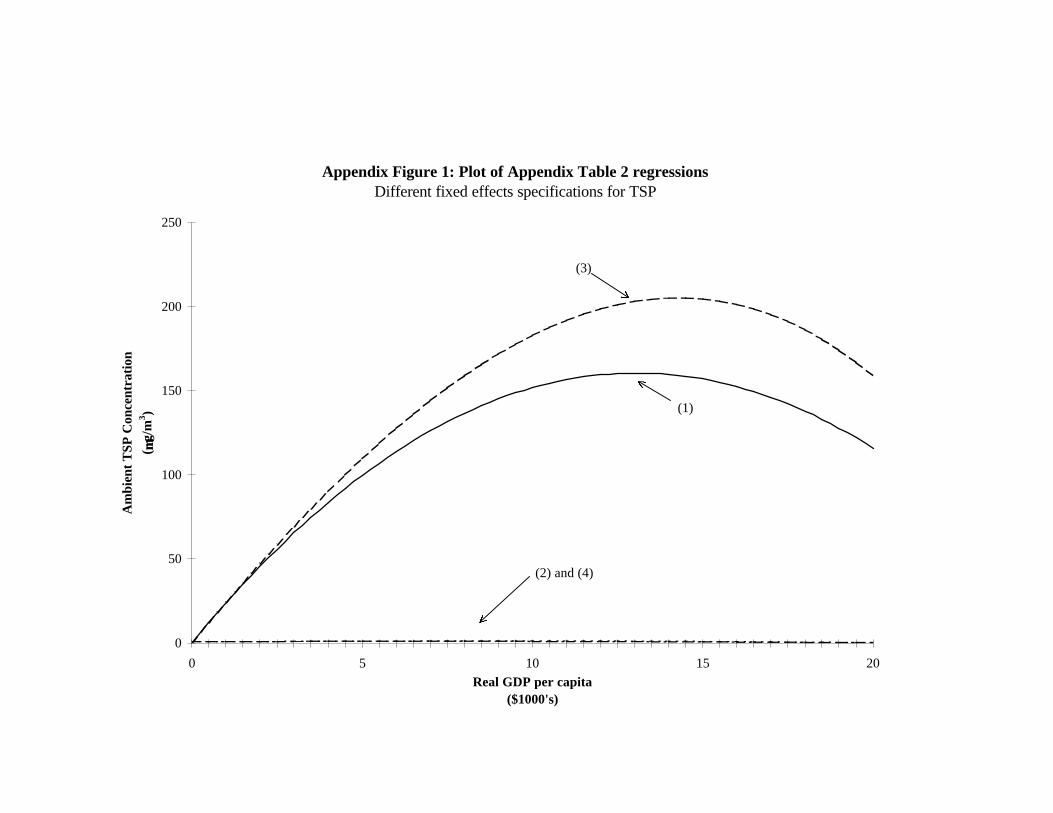
strongly for smoke and TSP. For these pollutants, we ran various specifications with the new AIRS

data, in a way similar to what we show in Tables 3 and 4 for SO2. (See Appendix Table 2 for the

results, and Appendix Figures 1 and 2 for the plots of those results.) For smoke and TSP the predicted

pollution-income paths have inverted-U-shapes, though the location and magnitudes of the peaks

depend on the specification.

Another means of demonstrating the uncertainty about the GDP-pollution relationship is to draw

confidence bands around the entire predicted path, rather than around individual coefficients. Since the

underlying variables, GDP, its polynomial, and lagged values, are correlated, the confidence bands will

be wider than might be inferred from the coefficients' standard errors. One approach would be to use

the joint confidence interval for all of the coefficients, not just the GDP coefficients. This approach might

be appropriate if we were interested in possible pollution paths for a country for which we knew the

values of the independent variables, but not the current pollution level. A second approach would be to

draw confidence bands for the future path of pollution, starting at current GDP, and assuming that we

know current pollution levels with certainty. This would result in a much narrower confidence band. We

11

compromise between these two approaches and ignore the uncertainty in all of the coefficients aside

from the GDP polynomials, including the intercept, and start at a GDP of zero.

Figure 2 depicts the confidence band for Grossman and Krueger’s (1995) SO2 specification,

column 1 of Table 3. These bands are based on bootstrapped 95 percent joint confidence intervals for

the GDP and lagged GDP polynomials. To interpret Figure 2, assume that the specification in column 1

of Table 3 is correct. In that case, we can say with 95 percent certainty that the "true" pollution-income

cubic equation falls within the indicated region. These confidence bands are obviously wide enough to

incorporate a variety of paths over the relevant range of GDP. We may have monotonically rising or

falling pollution, U-shapes or inverted-U-shapes, or more complicated relationships. Of course, the

confidence region shown assumes that the true relationship between GDP and pollution is the cubic

functional form estimated. If this is not correct, the true confidence band could be even wider.

Figure 3 depicts the 95 percent confidence band for the fixed-effects regression from column 4

of Table 4, constructed in a similar manner. Uncertainty about the shape of the pollution-income path is

equally apparent here. A variety of pollution-income paths may be described within the region depicted.

For smoke and TSP, the GDP coefficients have higher standard errors and the confidence bands (not

shown here) are wider than in the Figure 3 SO2 regressions.

5. Conclusion

In sum, for three important air pollutants, SO2, smoke, and TSP, we find that the estimated

relationship between pollution and GDP is sensitive to both sample and empirical specification. We

believe that, for these pollutants, there is little if any empirical support for the existence of an inverted-U-

shaped "environmental Kuznets curve." However, we believe this statement deserves at least two

qualifications.

12

First, there are theoretical arguments, such as those cited in our introduction, which suggest that

an inverted-U-shaped relationship may not only be possible, but in fact may be quite plausible. It may

well be the case that the existing data on a few pollutants, drawn from a few monitoring stations in a

small non-representative sample of cities over a relatively short period of time, is simply insufficient to

detect the true relationship between pollution and economic growth, should that be an inverted U.

Alternatively, most of the world's nations may not yet have reached income levels sufficient to generate

the turning points predicted by those theories.

The second point worth highlighting here is that while this paper shows that air quality does not

necessarily improve with economic growth, we have found no evidence in these data that environmental

quality necessarily declines with growth either. Our conclusion is simply that, for these pollutants, the

available empirical evidence cannot be used to support either the proposition that economic growth

helps the environment, or the proposition that it harms the environment.

References:

Andreoni, James and Arik Levinson. 1998. "The Simple Analytics of the Environmental KuznetsCurve." NBER Working Paper #6739.

Bartlett, Bruce. 1994. "The high cost of turning green." Wall Street Journal Sep 14, Sec. A, p 18 col.3.

Beckerman, W. 1992. "Economic growth and the environment: Whose growth? Whose environment?"World Development 20: 481-496.

Bennett, B. G., J.G. Kretzschmar, G.G. Akland, and H.W. de Koning. 1985. "Urban air pollutionworldwide: Results of the GEMS air monitoring project." Environmental Science andTechnology 19(4): 298-304.

Chaudhuri, S. and A. Pfaff. 1997. "Household income, fuel-choice and indoor air quality:Microfoundations of an environmental Kuznets curve" mimeo, Columbia University.

Grossman, G. and A. Krueger. 1995. "Economic growth and the environment" Quarterly Journal ofEconomics 110(2): 353-377.

Hilton, H. and A. Levinson. 1998. "Factoring the Environmental Kuznets Curve: Evidence FromAutomotive Lead Emissions" Journal of Environmental Economics and Management 35(2):126-141.

Holtz-Eakin, D. and T. Selden. 1995. "Stoking the fires? CO2 emissions and economic growth" Journalof Public Economics 57(1): 85-101.

Jaggers, Keith, and Ted Robert Gurr. 1995. “Polity III: Regime Change and Political Authority, 1800-1994” [Computer file]. 2nd ICPSR version. Ann Arbor, MI: Inter-university Consortium.

Jaeger, William. 1998. "A theoretical basis for the environmental inverted-U curve and implications forinternational trade." mimeo, Williams College.

Jones, Larry E. and Rodolfo E. Manuelli. 1995. "A positive model of growth and pollution controls"NBER working paper #5205.

Kuznets, Simon. 1955. "Economic growth and income inequality" American Economic Review 45(1):1-28.

Selden T. and D. Song. 1994. "Environmental quality and development: Is there a Kuznets curve for airpollution emissions?" Journal of Environmental Economics and Management 27: 147-162.

Selden T. and D. Song. 1995. "Neoclassical Growth, the J Curve for Abatement, and the Inverted UCurve for Pollution," Journal of Environmental Economics and Management 29(2): 162-68.

Shafik, N. 1994. "Economic development and environmental quality: An econometric analysis." Oxford

Economic Papers 46(1994): 201-227.

Stokey, Nancy L. 1998. "Are There Limits to Growth?" International Economic Review 39(1): 1-31.

Summers, Robert, and Alan Heston. 1991. "The Penn World Table (Mark 5): An expanded set of international comparisons, 1950-1988." Quarterly Journal of Economics 106(2): 327-68.

United Nations Environmental Programme (UNEP) and World Health Organization (WHO). 1983."Air quality in selected urban areas, 1979-1980." WHO Offset Publication 75. Geneva,Switzerland: WHO.

UNEP and WHO. 1984. Urban Air Pollution, 1973-1980. Geneva, Switzerland: WHO.

UNEP and WHO. 1992. Urban Air Pollution in Megacities of the World. Oxford, England: BlackwellReference.

UNEP and WHO. 1994. "Air pollution in the world’s megacities." Environment 36(2): 4-37.

World Bank. 1992. World Development Report 1992. New York: Oxford University Press.

Grossman and Krueger (1995) AIRSSO2 Obs. Mean S.D. Min. Max. Obs. Mean S.D. Min. Max.Median SO2 Conc. 1352 33.2 33.3 0 291 Not availableMean SO2 Conc. 1261 49.0 40.9 2.36 354 2401 49.4 50.9 0.782 1160GDP per Capita 1352 7.51 4.83 0.619 17.3 2381 9.43 5.73 0.765 18.13-yr-avg. lag GDP 1352 7.18 4.62 0.626 16.2 2389 9.10 5.56 0.779 18.010-yr-avg. lag GDP 2389 8.48 5.25 0.753 16.8Year 1352 1982 3.28 1977 1988 2401 1983 5.17 1971 1992Population Density 1352 3.35 4.56 0.00210 24.7 2401 2.75 3.99 0.00210 24.7Industrial 1352 0.291 0.455 0 1 2401 0.0875 0.283 0 1Residential 1352 0.360 0.480 0 1 2401 0.820 0.384 0 1Center City 1352 0.550 0.498 0 1 2401 0.862 0.345 0 1Coastal 1352 0.555 0.497 0 1 2401 0.565 0.496 0 1% GDP Invested 2381 23.1 5.49 4.20 41.5Trade Intensity 2381 42.5 32.9 8.84 262Democracy Index 2322 7.23 4.16 0 10Relative GDP 2381 1.121 0.910 -0.85 2.10

# sites 239 285# cities 77 102

# countries 42 45

TSP Obs. Mean S.D. Min. Max. Obs. Mean S.D. Min. Max.Median TSP Conc. 1021 147 127 0 715 Not availableMean TSP Conc. 1021 163 140 10.7 796 1092 177 146 9.80 796GDP per Capita 1021 8.11 5.99 0.619 17.3 1085 6.95 5.65 0.765 17.53-yr-avg. lag GDP 1021 7.71 5.72 0.626 16.2 1092 6.65 5.39 0.779 17.310-yr-avg. lag GDP 1092 6.11 4.95 0.753 15.9Year 1021 1982 3.29 1977 1988 1092 1984 4.88 1972 1992Population Density 1021 3.07 4.16 0.00210 24.7 1092 3.84 4.59 0.00150 24.7Industrial 1021 0.303 0.460 0 1 1092 0.0375 0.190 0 1Residential 1021 0.347 0.476 0 1 1092 0.920 0.271 0 1Center City 1021 0.467 0.499 0 1 1092 0.943 0.232 0 1Coastal 1021 0.529 0.499 0 1 1092 0.509 0.500 0 1Desert 1021 0.0411 0.199 0 1 1092 0.00916 0.0953 0 1% GDP Invested 1085 22.9 6.15 3.70 39.3Trade Intensity 1085 45.8 39.2 8.84 286Democracy Index 1063 5.66 4.55 0 10Relative GDP 1085 0.653 1.05 -1.08 2.03

# sites 161 149# cities 62 53

# countries 29 30

Smoke Obs. Mean S.D. Min. Max. Obs. Mean S.D. Min. Max.Median Smoke Conc. 488 42.2 42.6 0 312 Not availableMean Smoke Conc. 487 53.4 48.6 1.30 325 710 56.7 50.7 1.300 307GDP per Capita 488 6.81 3.00 1.34 12.2 687 6.78 3.22 1.293 13.53-yr-avg. lag GDP 488 6.61 2.88 1.25 11.4 687 6.60 3.05 1.187 12.410-yr-avg. lag GDP 687 6.22 2.84 1.117 11.6Year 488 1982 3.33 1977 1988 710 1982 4.89 1972 1992Population Density 488 3.64 5.30 0.00210 24.7 710 3.87 5.10 0.00210 24.7Industrial 488 0.275 0.447 0 1 710 0 0 0 0Residential 488 0.311 0.464 0 1 710 1 0 1 1Center City 488 0.568 0.496 0 1 710 1 0 1 1Coastal 488 0.607 0.489 0 1 710 0.513 0.500 0 1Desert 488 0.107 0.309 0 1 710 0.0465 0.211 0 1% GDP Invested 687 21.4 6.16 4.30 41.5Trade Intensity 687 56.0 37.9 8.96 210Democracy Index 646 6.13 4.36 0 10Relative GDP 687 0.975 0.540 -0.350 1.75

# sites 87 96# cities 30 32

# countries 19 21

Note: Grossman and Krueger (1995) include dummy variables for the type of monitoring device and for missing land-use and location information. These are not available in the AIRS data.

Table 1Comparison of summary statistics

Table 2Comparison of mean pollutant levels from AIRS with Grossman and Krueger's (1995) data

SO2 TSP Smoke

# of Paired City-Years 485 300 192

Correlation within Pairs 0.745 0.996 0.766

Mean of AIRS means 47.4 164 53.3

Mean of G&K means 47.2 164 56.2

Statistics for the ratio1 of paired pollution levels

Mean of the Ratio2 1.21 1.019 1.12

St. Dev. of the Ratio3 1.73 0.373 1.03

Min. Ratio 0.123 0.754 0.132

Max. Ratio 33.7 6.77 12.6

Notes:

1 Ratio refers to the ratio of the mean pollutant concentration for a given city-year in the AIRS data set to the mean concentration in the Grossman and Krueger data.

3 The expected standard deviation of the ratio is 0 if the data has not been altered and if our pairing is correct.

2 The expected mean of the ratio is 1 if the data has not been altered and if our pairing is correct.

Independent variables 1 2 3 4

GDP -7.37 -5.72 -29.9** -29.3**(9.15) (9.71) (10.2) (7.41)

(GDP)2 1.03 1.41 3.45** 4.06**(1.11) (1.20) (1.21) (0.769)

(GDP)3 -0.0337 -0.0543 -0.104* -0.127**(0.0384) (0.0415) (0.0407) (0.0232)

Lagged GDP 20.9* 14.7 10.6 14.1(9.75) (10.5) (11.0) (7.32)

(Lagged GDP)2 -3.22* -2.92* -1.40 -2.85**(1.26) (1.38) (1.40) (0.780)

(Lagged GDP)3 0.117* 0.109* 0.0382 0.0991**(0.0461) (0.0507) (0.0502) (0.0239)**

Year -1.40** -1.50** -0.475* -1.51**(0.218) (0.239) (0.240) (0.159)

Population Density 1.14 0.495 -0.647 -0.717(1.23) (0.551) (1.26) (1.05)

Industrial -0.485 -0.383 -34.6 -2.72(5.26) (6.96) (46.6) (24.9)

Residential -11.1* -6.69 -30.2 -5.39(4.85) (6.38) (33.3) (17.7)

Center City 3.06 11.4* 28.3 26.5(4.31) (5.71) (29.2) (15.5)

Coastal -12.7** -15.6* -22.8 -24.7*(3.78) (5.12) (11.8) (8.94)

# obs. 1352 1261 1403 2381# groups 239 233 227 282

R-squaredwithin 0.0953 0.0316 0.0990

between 0.140 0.0183 0.0340overall 0.273# 0.188 0.0425 0.0746

Turning PointsPeak $4,000 $3,718 $13,741 $20,081

(355) (649) (1419) (2592)Trough $13,534 $14,767 $7,145 $9,142

(599) (1297) (915) (877)Slopes

at $10,000 -5.30** -4.90** 2.10 0.721(0.609) (0.969) (1.334) (0.825)

at $12,000 -3.07** -3.75** 1.66 1.92*(0.91) (1.072) (1.44) (0.826)

Hausman Chi2 81.7** 223** 11.7 21.5*#

* p < 0.05** p < 0.01

Model Dependent variable Sample(1) median SO2 concentration Grossman and Krueger's (1995) data(2) mean SO2 concentration Grossman and Krueger's (1995) data(3) mean SO2 concentration New AIRS data: Only G&K's cities & years(4) mean SO2 concentration New AIRS data: All years & cities

Notes: Standard errors in parentheses. An overall constant term was included in all regressions. Grossman and Krueger (1995) also include dummy variables for monitor type and missing site information which were not significant.

Indicates adjusted r-squared. These results are estimated using Grossman and Krueger's Stata program, which does not provide within and between r-squareds

Table 3Effects of changes in the data on sulfur dioxide regressions

Table 4Effects of changes in the specification on sulfur dioxide regressions

Independent variables

1 2 3 4 5 6 7

GDP -33.3** -42.3** -19.5 -34.7** -39.2** -0.410** -0.302*(7.57 (6.50) (10.3) (6.79) (7.18) (0.139) (0.129)

(GDP)2 4.33** 4.67** 2.13* 3.78** 4.17** 0.0382* 0.0278*(0.781) (0.698) (0.848) (0.717) (0.781) (0.0151) (0.0136)

(GDP)3 -0.133** -0.133** -0.0610** -0.108** -0.126** -0.00110* -0.000697(0.0235) (0.0215) (0.0238) (0.0217) (0.0242) (0.000468) (0.000411)

Lagged GDP 7.86 16.3* 13.8* 20.3** 27.8** 0.488** 0.399**(7.46) (6.96) (6.73) (6.71) (6.86) (0.133) (0.127)

(Lagged GDP)2 -2.35** -2.86** -1.55 -3.22** -3.52** -0.0523** -0.0470**(0.787) (0.778) (0.797) (0.761) (0.822) (0.0160) (0.0144)

(Lagged GDP)3 0.0868** 0.0968** 0.0525 0.115** 0.129** 0.00177** 0.00150**(0.0241) (0.026) (0.0272) (0.0255) (0.0287) (0.000556) (0.000482)

Year -1.49** -1.20** -568** -2.28** -0.0541**(0.174) (0.215) (106) (0.266) (0.00503)

(Year)2 0.143**(0.0266)

Population Density 14.2** 8.92 524** 520** 586** 9.80** 9.23**(4.68) (4.80) (46.2) (46.1) (45.7) (0.887) (0.872)

Trade Intensity -0.582** -0.600** -0.450** -0.00931** -0.0110**(0.0868) (0.0876) (0.0915) (0.00177) (0.00166)

Democracy Index -3.63** -3.24** -3.09** -0.0400** -0.0390**(0.509) (0.499) (0.494) (0.00958) (0.00945)

Relative GDP -26.7(20.2)

Investment 0.661**(0.21)

# obs. 2381 2381 2314 2314 2314 2314 2314# groups 282 282 267 267 267 267 267

R'(squaredwithin 0.104 0.104 0.224 0.207 0.266 0.241 0.220

between 0.00220 0.00450 0.0196 0.0194 0.0178 0.122 0.121overall 0.0195 0.0328 0.0866 0.0866 0.0756 0.143 0.150

Turning PointsPeak $18,800 $22,500 $39,700 -$64,700 -$151,000 $3,770 $3,120

(1,460) (4,970) (49,300) (152,000) (764,000) (3,860) (2,388)Trough $9,790 $1,060 $5,650 $10,900 $8,300 $10,300 $12,800

(798) (835) (5,070) (683) (845) (1,654) (948)Slopes

at $10,000 0.251* -0.828 3.30 -1.33 2.47* -0.00346 -0.0458*(0.987) (1.08) (2.69) (1.06) (1.12) (0.0220) (0.0200)

at $12,000 2.07* 1.59 4.49 1.78 5.47** 0.0285 0.0161(0.931) (1.11) (2.37) (1.11) (1.19) (0.023) (0.0210)

Hausman Chi2 251** 22.7** 132** 155** 125** 635** 93.9*** p < 0.05

** p < 0.01

Model Dependent variable Description(1) mean SO2 concentration Short set of explanatory variables, 3'(year lags(2) mean SO2 concentration Longer lag structure but no additional regressors(3) mean SO2 concentration All explanatory variables(4) mean SO2 concentration Base model explanatory variables(5) mean SO2 concentration Year dummies(6) ln(mean SO2 concentration) Log dependent, year dummies(7) ln(mean SO2 concentration) Log dependent

Note: Standard errors in parentheses. An overall constant term was also included in all regressions.

Figure 1: Plot of Table 3 regressionsDifferent data sets for sulfur dioxide

-20

0

20

40

60

80

100

0 5 10 15 20Real GDP per capita

($1000's)

Am

bien

t SO

2 co

ncen

trat

ion

(µg/

m3 )

(1)

(3)(2)(4)

Figure 2: Regression estimate with 95% confidence bandsRandom effects, from Table 3, regression 2

-50

0

50

100

150

200

0 5 10 15 20

Real GDP per capita ($1000's)

Am

bien

t SO

2 co

ncen

trat

ion

( µµg/

m3 )

Figure 3: Regression estimate with 95% confidence bandsFixed effects, from Table 4, regression 4

-200

-150

-100

-50

0

50

100

150

200

0 5 10 15 20

Real GDP per capita ($1000's)

Am

bien

t SO

2 co

ncen

trat

ion

( µµg/

m3 )

Appendix Table 1Effects of changes in the data on TSP and smoke regressions

TSP Smoke

Independent variables 1 2 3 4

GDP 17.4 22.3 24.5 18.4(21.5) (21.1) (20.9) (21.1)

(GDP)2 -0.922 -2.02 -7.64* -2.22(2.65) (2.34) (3.58) (3.17)

(GDP)3 0.0136 0.0595 0.443** 0.102(0.0902) (0.0737) (0.171) (0.139)

Lagged GDP -60.7** -43.6* 12.6 62.0**(23.3) (20.9) (22.0) (23.2)

(Lagged GDP)2 4.35 3.45 3.44 -9.07*(3.12) (2.40) (3.96) (3.67)

(Lagged GDP)3 -0.115 -0.0951 -0.313 0.373*(0.112) (0.0783) (0.199) (0.170)

Year 0.744 -1.84** -1.23** -2.29**(0.631) (0.462) (0.358) (0.254)

Population Density -0.699 4.04* 2.39** 1.60(1.40) (1.83) (0.853 (0.952)

Industrial 23.8 -26.4 -11.6 (dropped)(17.4) (61.1) (10.7)

Residential 7.35 -98.0* -13.9 4450**(16.4) (38.9) (9.36) (502)

Center City 26.2 -149** 4.05 (dropped)(14.5) (42.2) (8.86)

Coastal -21.1 -40.6* -33.7** -34.2**(12.1) (17.2) (8.35) (9.16)

Desert 162** 252** 7.08 52.8*(26.1) (58.1) (11.2) (25.2)

# obs. 1021 1085 488 687# groups 148 92

R-squaredwithin 0.0195 0.190

between 0.501 0.193overall 0.485# 0.526 0.312# 0.270

Turning PointsPeak none none $6,194 $5,399

$539 $237Trough none none $15,455 $10,447

$6,598 $452Slopes

at $10,000 -5.16 -3.27 -8.05 -2.93(5.16) (2.45) (12.74) (2.64)

at $12,000 -4.81* -2.24 -7.78 14.6*(2.08) (2.12) (8.65) (6.48)

Hausman Chi2 122** 151** 4.81 24.6**#

* p < 0.05** p < 0.01

Model Dependent variable Description(1) median TSP concentration Grossman and Krueger's (1995) Results(2) mean TSP concentration Their model using the new AIRS data(3) mean smoke concentration Grossman and Krueger's (1995) Results(4) median smoke concentration Their model using the new AIRS data

Notes: Standard errors in parentheses. An overall constant term was included in all regressions. Grossman and Krueger (1995) also include dummy variables for monitor type and missing site information, none of which were significant.

Indicates adjusted r-squared. These results are estimated using Grossman and Krueger's Stata program, which does not provide within and between r-squareds.

Appendix Table 2Effects of changes in the specification on TSP and smoke regressions

TSP Smoke

Independent variables 1 2 3 4 5 6 7 8GDP 60.6** 0.165 54.5** 0.161 55.6** 0.975** 68.2** 1.01**

(20.1) (0.103) (20.7) (0.107) (19.8) (0.327) (21.8) (0.353)

(GDP)2 -3.58 -0.00402 -2.60 -0.00356 -7.13* -0.149** -9.24** -0.157**(2.30) (0.0118) (2.39) (0.0123) (2.89) (0.0479) (3.18) (0.0515)

(GDP)3 0.0759 0.0000549 0.0347 -0.00000228 0.271* 0.00638** 0.363** 0.00677**(0.0730) (0.000375) (0.0762) (0.000393) (0.125) (0.00207) (0.137) (0.00222)

Lagged GDP -35.9 -0.157 -30.0 -0.164 -8.33 -0.846* -47.8* -1.47**(20.6) (0.105) (20.8) (0.107) (21.59) (0.357) (24.0) (0.387)

(Lagged GDP)2 2.62 0.00663 2.19 0.0124 0.959 0.138* 8.29* 0.251**(2.59) (0.0133) (2.71) (0.0140) (3.45) (0.0573) (3.93) (0.0637)

(Lagged GDP)3 -0.0750 -0.000357 -0.0553 -0.000571 -0.0593 -0.00709* -0.396* -0.0123**(0.0934) (0.000479) (0.0985) (0.000508) (0.170) (0.00282) (0.190) (0.00308)

Year -1.62 -0.00642 0.639 0.00442(0.836) (0.00429) (0.742) (0.0123)

Population Density -206 -0.153 -95.7 0.597 -1080** -10.5 -526.2281 -0.034866(139) (0.715) (143) (0.735) (325) (5.39) (342) (5.53)

Trade Intensity 0.478 0.00138 0.402 0.000944 0.0986 0.000886 0.288 0.00619*(0.267) (0.00137) (0.276) (0.00142) (0.146) (0.00241) (0.162) (0.00262)

Democracy Index -8.72** -0.0394** -9.70** -0.0466** -2.94** -0.0337** -2.39** -0.0190(2.21) (0.0113) (2.23) (0.0115) (0.642) (0.0106) (0.684) (0.0111)

# obs. 1056 1056 1056 1056 646 646 646 646# groups 144 144 144 144 89 89 89 89

R-squaredwithin 0.114 0.190 0.162 0.226 0.216 0.136 0.287 0.250

between 0.0981 0.178 0.143 0.0426 0.0414 0.0340 0.0337 0.0110overall 0.156 0.247 0.240 0.0642 0.0761 0.0625 0.0686 0.0489

Turning PointsPeak $13,057 $7,013 $14,291 $10,082 $5,258 $4,227 $7,697 $7,591

(2384) (3147) (2292) (1370) (586) (1599) (1342) (1141)Trough $764,867 -$1,247 -$27,674 $179 $14,146 -$14,284 -$27,136 $3,705

(53176425) (12685) (94255) (4385) (3543) (64509) (132202) (1229)Slopes

at $10,000 5.71 -0.0304 10.0* 0.00139 -12.5* -0.299** -8.33 -0.251**(4.11) (0.0211) (4.54) (0.0234) (5.71) (0.095) (5.96) (0.0970)

at $12,000 1.97 -0.0598** 5.63 -0.0390 -9.20 -0.435* -16.4 -0.605**(3.99) (0.0205) (4.29) (0.0221) (10.9) (0.181) (11.1) (0.180)

Hausman Chi2 61.6* 35.4** 68.3** 79.2** 37.8** 32.7** 223** 19.9

* p < 0.05** p < 0.01

Model Dependent variable Model1 mean TSP concentration Base model explanatory variables2 ln(mean TSP concentration) Base model explanatory variables3 mean TSP concentration Year dummies4 ln(mean TSP concentration) Year dummies5 mean smoke concentration Base model explanatory variables6 ln(mean smoke concentration) Base model explanatory variables7 mean smoke concentration Year dummies8 ln(mean smoke concentration) Year dummies

Note:Standard errors in parentheses. An overall constant term was also included in each model.

Appendix Figure 1: Plot of Appendix Table 2 regressionsDifferent fixed effects specifications for TSP

0

50

100

150

200

250

0 5 10 15 20Real GDP per capita

($1000's)

Am

bien

t T

SP C

once

ntra

tion

( µµg/

m3 ) (1)

(2) and (4)

(3)

Appendix Figure 2: Plot of Appendix Table 2 regressionsDifferent fixed effects specifications for smoke

-300

-250

-200

-150

-100

-50

0

50

100

150

200

0 5 10 15 20

Real GDP per capita ($1000's)

Am

bien

t Sm

oke

Con

cent

rati

on

( µµg/

m3 )

(5)

(6) and (8)

(7)