university of minnesota - penn engineering - …aribeiro/preprints/t_2005_ribeiro.pdfuniversity of...
TRANSCRIPT

UNIVERSITY OF MINNESOTA
This is to certify that I have examined this copy of a Master’s thesis by
Alejandro Ribeiro
and have found that it is complete and satisfactory in all respects, and that any and allrevisions required by the final examining committee have been made.
Name of Faculty Advisor(s)
Signature of Faculty Advisor(s)
Date
GRADUATE SCHOOL
Distributed Quantization-Estimation
for Wireless Sensor Networks
A THESIS
SUBMITTED TO THE FACULTY OF THE GRADUATE SCHOOL
OF THE UNIVERSITY OF MINNESOTA
BY
Alejandro Ribeiro
IN PARTIAL FULFILLMENT OF THE REQUIREMENTS
FOR THE DEGREE OF
MASTER OF SCIENCE
Professor Georgios B. Giannakis, Advisor
August 2005

c©Alejandro Ribeiro 2006

i
Distributed Quantization-Estimation
for Wireless Sensor Networks
Abstract:At the crossroad of sensing, control and wireless communications, wireless sensor net-
works (WSNs), whereby large numbers of individual nodes collaborate to monitor and con-trol environments, have emerged in recent years along with the field of distributed signalprocessing. This thesis studies the intertwining between quantization and estimation thatarises due to the distributed nature of WSNs. Given that each sensor has available onlypart of the measurements parameter estimation requires quantization of the original obser-vations, transforming the problem into one of estimation based on quantized observations– certainly different from estimation based on the analog-amplitude observations.
This intertwining is studied in a number of setups with an eye towards realistic sce-narios. We start with a simple mean location deterministic parameter estimation problem,in the presence of additive white Gaussian noise which we follow with generalizations todeterministic parameter estimation for pragmatic signal models. Among this class of signalmodels we consider i) known univariate but generally non-Gaussian noise probability den-sity functions (pdfs); ii) known noise pdfs with a finite number of unknown parameters; iii)completely unknown noise pdfs; and iv) practical generalizations to multivariate and pos-sibly correlated pdfs. Within a different paradigm, we also derive and analyze distributedstate estimators of dynamical stochastic processes. Following a Kalman filtering (KF) ap-proach, we develop recursive algorithms for distributed state estimation based on the signof innovations (SOI).
Surprisingly, in all scenarios considered we reveal two common properties: i) the per-formance of estimators based on quantization to a few bits per sensor can come very closeto the performance of estimators based on the analog-amplitude observations; and ii) thecomplexity of optimal estimators based on quantized observations is low even though quan-tization leads to a discontinuous signal model.

ii
Contents
Abstract i
List of Figures v
1 Wireless Sensor Networks 11.1 Distributed Estimation with WSNs . . . . . . . . . . . . . . . . . . . . . . . 21.2 WSN topologies . . . . . . . . . . . . . . . . . . . . . . . . . . . . . . . . . . 51.3 Some motivating applications . . . . . . . . . . . . . . . . . . . . . . . . . . 6
1.3.1 Estimating a vector wind flow . . . . . . . . . . . . . . . . . . . . . . 71.3.2 Target tracking with SOI-EKF . . . . . . . . . . . . . . . . . . . . . 8
1.4 The thesis in context . . . . . . . . . . . . . . . . . . . . . . . . . . . . . . . 12
2 Mean-location in additive white Gaussian noise 142.1 Introduction . . . . . . . . . . . . . . . . . . . . . . . . . . . . . . . . . . . . 142.2 Problem statement . . . . . . . . . . . . . . . . . . . . . . . . . . . . . . . . 152.3 MLE based on binary observations: common thresholds . . . . . . . . . . . 162.4 MLE based on binary observations: non-identical thresholds . . . . . . . . . 19
2.4.1 Selecting the parameters (τ , ρ) . . . . . . . . . . . . . . . . . . . . . 212.4.2 An achievable upper bound on BW (τ ,ρ) . . . . . . . . . . . . . . . . 252.4.3 Algorithmic Implementation . . . . . . . . . . . . . . . . . . . . . . . 26
2.5 Relaxing the Bandwidth Constraint . . . . . . . . . . . . . . . . . . . . . . 282.5.1 Optimum threshold spacing . . . . . . . . . . . . . . . . . . . . . . . 31
2.6 Quantized sample mean estimator . . . . . . . . . . . . . . . . . . . . . . . 322.7 Numerical results . . . . . . . . . . . . . . . . . . . . . . . . . . . . . . . . . 34
2.7.1 Designing (τ , ρ) . . . . . . . . . . . . . . . . . . . . . . . . . . . . . 342.7.2 Estimation with 1 bit per sensor . . . . . . . . . . . . . . . . . . . . 342.7.3 Comparison with deterministic control signals . . . . . . . . . . . . . 36
2.8 Appendices . . . . . . . . . . . . . . . . . . . . . . . . . . . . . . . . . . . . 39

CONTENTS iii
2.8.1 Proof of Proposition 2.3 . . . . . . . . . . . . . . . . . . . . . . . . . 392.8.2 Proof of Theorems 2.1 and 2.2 . . . . . . . . . . . . . . . . . . . . . 392.8.3 Proof of Proposition 2.4 . . . . . . . . . . . . . . . . . . . . . . . . . 422.8.4 Proof of Proposition 2.5 . . . . . . . . . . . . . . . . . . . . . . . . . 432.8.5 Proof of Proposition 2.7 . . . . . . . . . . . . . . . . . . . . . . . . . 46
3 Distributed batch estimation based on binary observations 473.1 Introduction . . . . . . . . . . . . . . . . . . . . . . . . . . . . . . . . . . . . 473.2 Problem Statement . . . . . . . . . . . . . . . . . . . . . . . . . . . . . . . . 483.3 Scalar parameter estimation – Parametric Approach . . . . . . . . . . . . . 49
3.3.1 Known noise pdf . . . . . . . . . . . . . . . . . . . . . . . . . . . . . 493.3.2 Known Noise pdf with Unknown Variance . . . . . . . . . . . . . . . 523.3.3 Dependent binary observations . . . . . . . . . . . . . . . . . . . . . 55
3.4 Scalar parameter estimation – Unknown noise pdf . . . . . . . . . . . . . . 573.4.1 Independent binary observations . . . . . . . . . . . . . . . . . . . . 593.4.2 Dependent binary observations . . . . . . . . . . . . . . . . . . . . . 623.4.3 Practical Considerations . . . . . . . . . . . . . . . . . . . . . . . . . 64
3.5 Vector parameter Generalization . . . . . . . . . . . . . . . . . . . . . . . . 653.5.1 Colored Gaussian Noise . . . . . . . . . . . . . . . . . . . . . . . . . 67
3.6 Simulations . . . . . . . . . . . . . . . . . . . . . . . . . . . . . . . . . . . . 713.6.1 Scalar parameter estimation . . . . . . . . . . . . . . . . . . . . . . . 713.6.2 Vector Parameter Estimation – A Motivating Application . . . . . . 74
3.7 Appendices . . . . . . . . . . . . . . . . . . . . . . . . . . . . . . . . . . . . 763.7.1 Proofs of Lemma 3.1 and Proposition 3.2 . . . . . . . . . . . . . . . 763.7.2 Proofs of Lemma 3.2 and Proposition 3.4 . . . . . . . . . . . . . . . 773.7.3 Proof of Proposition 3.5 . . . . . . . . . . . . . . . . . . . . . . . . . 79
4 Distributed state estimation using the sign of innovations 814.1 Introduction . . . . . . . . . . . . . . . . . . . . . . . . . . . . . . . . . . . . 814.2 Problem statement and preliminaries . . . . . . . . . . . . . . . . . . . . . . 83
4.2.1 The Kalman filter benchmark . . . . . . . . . . . . . . . . . . . . . . 874.3 State estimation using the sign of innovations . . . . . . . . . . . . . . . . . 88
4.3.1 Exact MMSE Estimator . . . . . . . . . . . . . . . . . . . . . . . . . 884.3.2 Approximate MMSE estimator . . . . . . . . . . . . . . . . . . . . . 91
4.4 Vector state - vector observation case . . . . . . . . . . . . . . . . . . . . . . 954.5 Performance analysis . . . . . . . . . . . . . . . . . . . . . . . . . . . . . . . 984.6 Simulations . . . . . . . . . . . . . . . . . . . . . . . . . . . . . . . . . . . . 103

CONTENTS iv
4.6.1 Target tracking with SOI-EKF . . . . . . . . . . . . . . . . . . . . . 1064.7 Appendix – Proof of (4.20) . . . . . . . . . . . . . . . . . . . . . . . . . . . 109
5 Conclusions and Future Work 1125.1 Future research . . . . . . . . . . . . . . . . . . . . . . . . . . . . . . . . . . 114
5.1.1 Maximum a posteriori estimation with binary observations . . . . . 1155.1.2 Extensions of the SOI-KF . . . . . . . . . . . . . . . . . . . . . . . . 115
Bibliography 117

v
List of Figures
1.1 WSN with a Fusion Center: the sensors act as data gathering devices. . . . 51.2 Ad hoc WSN: the network itself is in charge of estimation . . . . . . . . . . 61.3 The wind v incises over a certain sensor capable of measuring the normal
component of v. . . . . . . . . . . . . . . . . . . . . . . . . . . . . . . . . . 71.4 Average variance for the components of v. The empirical as well as the
bound (1.6) are compared with the analog observations based MLE (v =(1, 1), σ = 1). . . . . . . . . . . . . . . . . . . . . . . . . . . . . . . . . . . . 9
1.5 Target tracking with EKF and SOI-EKF yield almost identical estimates.The scheduling algorithm works in cycles of duration T . At the beginning ofthe cycle, we schedule the sensor Sk closest to the estimate x(n|n− 1), nextthe second closest and so on until we complete the cycle (T = 4, Ts = 1s,L = 2km, K = 100, α = 3.4 σu = 0.2m, σv = 1). . . . . . . . . . . . . . . . 10
1.6 Standard deviation of the estimates in Fig. 1.5 are in the order of 5m-10mfor both filters. . . . . . . . . . . . . . . . . . . . . . . . . . . . . . . . . . . 11
2.1 CRLB and Chernoff bound in (2.13) as a function of the distance between τc
and θ measured in AWGN standard deviation (σ) units. . . . . . . . . . . . 182.2 MLE in (2.6) based on binary observations performs close to the clairvoyant
sample mean estimator when θ is close to the threshold defining the binaryobservation (σ = 1, τc = 0, and θ = 1). . . . . . . . . . . . . . . . . . . . . . 19
2.3 Variance of the estimator relying on the whole sequence of binary observa-tions. The room for improved performance once τ < σ is small. . . . . . . . 29
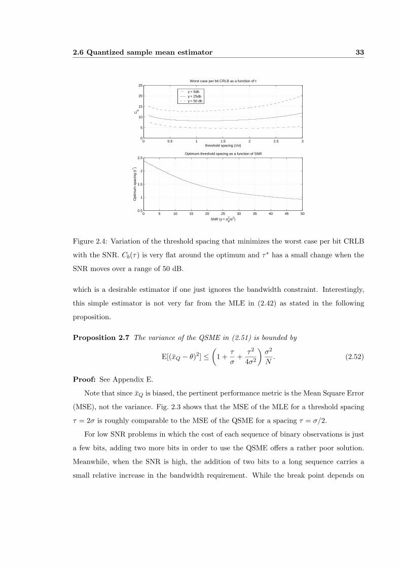
2.4 Variation of the threshold spacing that minimizes the worst case per bitCRLB with the SNR. Cb(τ) is very flat around the optimum and τ∗ has asmall change when the SNR moves over a range of 50 dB. . . . . . . . . . . 33

LIST OF FIGURES vi
2.5 Gaussian noise and Gaussian-shaped weight function. Although a thresholdspacing τ = σ reduces the approximation error to almost zero, a spacingτ = 2σ is good enough in practice (σ = 1, and σθ = 2). . . . . . . . . . . . . 35
2.6 Gaussian noise and Uniform weight function. A threshold spacing τ = σ
has smaller MSE but a spacing τ = 2σ is better in most of the non-zeroprobability interval (σ = 1, and prior U[-7,7]). . . . . . . . . . . . . . . . . . 35
2.7 Gaussian noise and Gaussian weight function. With a threshold spacingτ = 2σ we achieve a good approximation to the minimum asymptotic averagevariance (σ = 1, τ = 2, and σθ = 2). . . . . . . . . . . . . . . . . . . . . . . 36
2.8 The average variance of the optimum set (τ , ρ) found as the solution of (2.37),yields a noticeable advantage over the use of equispaced equal frequencythresholds as defined by (2.55) (σ = 1, τ = 2, and σθ = 2). . . . . . . . . . 37
3.1 Per bit CRLB when the binary observations are independent (Section 3.3.2)and dependent (Section 3.3.3), respectively. In both cases, the varianceincrease with respect to the sample mean estimator is small when the σ-distances are close to 1, being slightly better for the case of dependent binaryobservations (Gaussian noise). . . . . . . . . . . . . . . . . . . . . . . . . . . 55
3.2 When the noise pdf is unknown numerically integrating the CCDF using thetrapezoidal rule yields an approximation of the mean. . . . . . . . . . . . . 58
3.3 The vector of binary observations b takes on the value {β1, β2} if and onlyif x(n) belongs to the region B{β1,β2}. . . . . . . . . . . . . . . . . . . . . . 65
3.4 Selecting the regions Bk(n) perpendicular to the covariance matrix eigenvec-tors results in independent binary observations. . . . . . . . . . . . . . . . . 67
3.5 Noise of unknown power estimator. The CRLB in (3.15) is an accurate pre-diction of the variance of the MLE estimator (3.14); moreover, its varianceis close to the clairvoyant sample mean estimator based on the analog obser-vations (σ = 1, θ = 0, Gaussian noise). . . . . . . . . . . . . . . . . . . . . . 72
3.6 Universal estimator introduced in Section 3.4. The bound in (3.39) overes-timates the real variance by a factor that depends on the noise pdf (σ = 1,T = 5, θ chosen randomly in [−2, 2]) . . . . . . . . . . . . . . . . . . . . . . 73
3.7 The vector flow v incises over a certain sensor capable of measuring thenormal component of v. . . . . . . . . . . . . . . . . . . . . . . . . . . . . 73
3.8 Average variance for the components of v. The empirical as well as thebound (3.68) are compared with the analog observations based MLE (v =(1, 1), σ = 1). . . . . . . . . . . . . . . . . . . . . . . . . . . . . . . . . . . . 74

LIST OF FIGURES vii
4.1 Ad hoc WSN: the network itself is in charge of tracking the state x(n) . . . 834.2 WSN with a Fusion Center: the sensors act as data gathering devices. . . . 864.3 The MSEs, tr[M(Ts; n|n)] of the estimator and tr[M(Ts;n|n − 1)] of the
predictor converge to the continuous-time MSE tr[Mc(nTs)] as Ts decreases(Ac(t) = I, hc(t) = [1, 2]T , Cuc(t) = I, and σ2
vc(t) = 1). . . . . . . . . . . . 103
4.4 The MSE tr[M(Ts; n|n)] of the SOI-KF and the MSE tr[Mπ/2(Ts; n|n)] of the(π/2)-KF are indistinguishable for small Ts; as Ts increases there is a notice-able but still small difference. The penalty with respect to tr[MK(Ts; n|n)] issmall for moderate Ts (Ac(t) = I, hc(t) = [1, 2]T , Cuc(t) = I, and σvc(t) = 1).104
4.5 SOI-KF compared with the (π/2)-KF. The filtered MSEs of the two filtersare indistinguishable for small Ts, but as Ts becomes large, the (π/2)-KFis not a good predictor of the SOI-KF’s performance (β1 = 0.1, β2 = 0.2,σ2
u = 1 and σ2v = 1). . . . . . . . . . . . . . . . . . . . . . . . . . . . . . . . 105
4.6 SOI-KF compared with KF: even for moderate values of Ts, the performancepenalty is small (β1 = 0.1, β2 = 0.2, σ2
u = 1 and σ2v = 1). . . . . . . . . . . . 106
4.7 Target tracking with EKF and SOI-EKF yield almost identical estimates.The scheduling algorithm works in cycles of duration T . At the beginning ofthe cycle, we schedule the sensor Sk closest to the estimate x(n|n− 1), nextthe second closest and so on until we complete the cycle (T = 4, Ts = 1s,L = 2km, K = 100, α = 3.4 σu = 0.2m, σv = 1). . . . . . . . . . . . . . . . 108
4.8 Standard deviation of the estimates in Fig. 4.7 are in the order of 5m-10mfor both filters. . . . . . . . . . . . . . . . . . . . . . . . . . . . . . . . . . . 108
1
Chapter 1
Wireless Sensor Networks
Recent years have witnessed the evolution of wireless sensor networks (WSNs), which in
broad terms can be defined as a group of wireless sensors. A wireless sensor, in turn,
is a signal processing device capable of sensing physical variables, acting in the physical
environment and communicating with other devices over a wireless channel. By touching
upon the centuries old fields of sensing and control and the decades old field of wireless
communications the former definition hardly contains any novel idea at all; however, it is
the combination of these fields that has led to a whole new set of applications.
Indeed, the major ability that has been rare so far and WSNs have, is that the addition
of wireless communication abilities to the sensors enables distributed sensing and control.
While this may not look like a significant difference, there are a number of applications that
become possible or are simpler to perform with a distributed WSN. Consider as a typical
example, habitat monitoring, where we want to sense variables of pertinent interest to a
particular environment, e.g., air quality indicators in a certain neighborhood. The difficulty
for a centralized sensing system is that there is no single indicator but a space varying
field. This field can be more easily estimated by a distributed network of sensors. Yet
another canonical example is target tracking. While a centralized tracker will do just fine,
a distributed network can collect more accurate observations given the greater likelihood
a sensor has to be close to the target. Even if we could spend pages describing potential
applications, the important point here is that the physical world is inherently distributed and

1.1 Distributed Estimation with WSNs 2
if we want to sense and take actions in it, the ultimate goal is a distributed sensing/control
network. And that is what a WSN is.
Trying to keep this introduction as general as possible we have omitted a number of
assumptions that are customary in WSN research and that will be considered integral to our
WSN setup in the rest of the dissertation. Besides its already described abilities, a sensor is
supposed to be a relatively inexpensive device. Thus, the quality of the observations it makes
is considered low, and its processing capabilities limited. Moreover, it is a usual requirement
to have severe power and bandwidth constraints being not rare the assumption that a sensor
can only transmit a few bits and be active a few minutes per hour. The network, on the
other hand, is considered to consist of a large number of sensors randomly distributed in
the area of interest. These properties ensure that WSNs can be easily deployed, are robust
to failures and can operate on limited energy for long periods of time.
1.1 Distributed Estimation with WSNs
Foremost among the tasks performed by WSNs is the observation of physical phenomena,
either a goal in itself in e.g., environmental monitoring applications or the first step in
distributed control. While a number of tools in the fields of statistics and information theory
among others, have been developed over the years, the unique characteristics of WSNs
require rethinking of many of the algorithms traditionally used for estimation. Indeed, the
distributed nature of the observations necessitates transmission of the individual sensors’
data; moreover, the power/bandwidth available for transmission and signal processing is
severely limited. To complicate matters even more the parametric data model used and
the knowledge of sensor noise distributions are not easy to characterize; observations taken
by (small, cheap) sensors are very noisy; and the WSN size and topology may change
dynamically.
To appreciate the challenges implied by these properties, consider a customary mean-
location parameter estimation problem in which we estimate a parameter in additive zero-
mean noise. The distributed nature of the observations dictates quantization of the original
observations prior to digital transmission transforming the estimation problem into one
1.1 Distributed Estimation with WSNs 3
of estimation based on the quantized digital messages –certainly different from estimation
based on the original analog-amplitude observations. Besides, the severe bandwidth/power
constraint requires these messages to contain only a few bits and the lack of an accurate
data/noise model preempts application of optimum estimation algorithms. Thus, estimation
with WSNs requires studying the intertwining between quantization and estimation based
on severely quantized data in possibly unknown data/noise models.
The main focus of the present thesis is to study the problem of distributed estima-
tion using a WSN with particular emphasis in the intertwining between quantization and
estimation.
We begin by studying distributed mean-location parameter estimation in the presence
of additive white Gaussian noise (AWGN) in Chapter 2. We seek Maximum Likelihood
Estimators (MLE) based on quantized observations and benchmark their variances with the
Cramer-Rao Lower Bound (CRLB) that, at least asymptotically, is achieved by the MLE.
We show that the deciding factor in the choice of the estimator is the relation between the
dynamic range of the parameter and the observation noise variance. When the dynamic
range of the parameter is small or comparable with the noise variance, we introduce a
class of maximum likelihood estimators that require transmitting just one bit per sensor
to achieve an estimation variance close to that of the (clairvoyant) sample mean estimator.
When the dynamic range is comparable or larger than the noise standard deviation, we
show that an optimum quantization step exists to achieve the best possible variance for a
given bandwidth constraint. We also establish that in this case the sample mean estimator
formed by quantized observations is preferable for complexity reasons. We finally touch
upon algorithm implementation issues and guarantee that all the numerical maximizations
required by the proposed estimators are concave implying that low complexity optimization
algorithms like e.g., Newton’s method converge to the unique global maximum.
One of the most important conclusions of Chapter 2 is that when the parameter’s dy-
namic range is comparable with the noise variance, the variance performance of a estimator
based on the transmission of a single bit per observation is within a small factor of the
variance of the clairvoyant sample mean estimator. The goal of Chapter 3 is to show that

1.1 Distributed Estimation with WSNs 4
this fundamental property extends to more pragmatic models. Indeed, we show in Chapter
3 that for a large class of distributed estimation problems, even a single bit per sensor
can afford minimal increase in estimation variance. Among these pragmatic signal mod-
els, we consider: i) known univariate but generally non-Gaussian noise probability density
functions (pdfs); ii) known noise pdfs with a finite number of unknown parameters; iii)
completely unknown noise pdfs; and iv) practical generalizations to multivariate and pos-
sibly correlated pdfs. Quite surprisingly, besides the small performance penalty paid in all
of these scenarios it also turns out that the MLE can either be obtained in closed form or
as the (unique) maximum of a concave function. Corroborating our theoretical findings we
consider a motivating application entailing distributed parameter estimation where a WSN
is used for habitat monitoring.
A conclusion of Chapters 2 and 3 is the possibility of accurate parameter estimation
based on severe quantization to a single bit per observation when we have reasonably ac-
curate prior knowledge about the parameter. A problem in which this is indeed true is
state estimation of dynamical stochastic processes, in which the state prediction based on
past observations can be used to quantize the current observation. This is the subject of
Chapter 4 where we derive and analyze distributed state estimators of dynamical stochastic
processes, whereby low communication cost is effected by requiring the transmission of a
single bit per observation. Following a Kalman filtering (KF) approach, we develop re-
cursive algorithms for distributed state estimation based on the sign of innovations (SOI).
Even though SOI-KF can afford minimal communication overhead, we prove that in terms
of performance and complexity it comes very close to the clairvoyant KF which is based on
the analog-amplitude observations. Reinforcing our conclusions, we show that the SOI-KF
applied to distributed target tracking based on distance only observations yields accurate
estimates at low communication cost.
It is worth noting that the flow of the thesis is not only towards increasingly complex
problems but towards more realistic ones. As results in Chapter 2 are insightful but of little
practical significance, we introduce the pragmatic signal models of Chapter 3. Alas, both
Chapters left unaddressed the issue of prior knowledge. That is addressed in Chapter 4,

1.2 WSN topologies 5
+ + +x(0) v(0)
. . . .
S0 S1 Sk
m(0) m(1) m(k)
x(1) v(1) x(k) v(k)
F u s i o n C e n t e r
f(n)
P l a n t
Figure 1.1: WSN with a Fusion Center: the sensors act as data gathering devices.
where a practical state estimation algorithm based on binary SOI observations is developed,
analyzed and tested.
1.2 WSN topologies
Two different WSN topologies characterized by the presence or absence of a fusion center
(FC) are considered in this thesis. When an FC is present, the WSN is termed hierarchical
in the sense that sensors act as information gathering devices for the FC that is in charge
of processing this information. A hierarchical WSN used to estimate parameters of a given
plant is shown in Fig. 1.1. Sensor Sk collects information about the plant and encodes
this information on the message m(k) that it communicates to the FC. The FC collects
information from different sensors that it later processes to estimate the plant parameters
of interest. This topology may also include a feedback channel from the FC to the sensor
in which at time slot n messages f(n) are broadcast to the sensors.
In ad-hoc WSNs, the network itself is responsible for processing the collected informa-
tion, and to this end sensors communicate with each other through the shared wireless
medium; see Fig. 1.2. We assume that the message m(k) sent by sensor Sk is received by
all other sensors, using a forwarding mechanism the details of which go beyond the scope

1.3 Some motivating applications 6
+ + +x(0) w(0)
. . . .
S0 S1 Sk
x(1) w(1) x(k) w(k)
P l a n t
m(0) m(1) m(k)
Figure 1.2: Ad hoc WSN: the network itself is in charge of estimation
of the present thesis.
Though not explicitly addressed in this thesis, hybrid models in which some low level
processing is performed by the network and high level ones by the FC are also common in
practice.
An important distinction between ad-hoc and hierarchical architectures pertains to the
amount of information available to each sensor. In ad-hoc WSNs, the messages m(k) perco-
late through all sensors. Consequently, in addition to the information collected locally, the
sensors have available plant observations collected by other sensors. In hierarchical WSNs,
on the other hand, the information is sent to the FC and each sensor has available only the
information collected locally. A third level of information availability arises in hierarchical
WSN with a feedback channel in which the sensors receive plant information via feedback
from the FC.
In this work, we assume that the messages m(k) and f(n) are correctly received by either
the sensors or the FC, which requires deployment of sufficiently powerful error control codes.
1.3 Some motivating applications
This section presents two motivating applications that illustrate the type of problems to
which results in this thesis are applicable. It also serves as a prelude for the results that
will be derived in ensuing chapters.

1.3 Some motivating applications 7
x0
x1
φ (n)
n
v
Figure 1.3: The wind v incises over a certain sensor capable of measuring the normal
component of v.
1.3.1 Estimating a vector wind flow
Consider the problem of estimating a wind flow (velocity and direction) using incidence
observations. With reference to Fig. 1.3, consider the flow vector v := (v0, v1)T , and a
sensor positioned at an angle φ(n) with respect to a known reference direction. The so
called incidence observations {x(n)}N−1n=0 measure the component of the flow normal to the
corresponding sensor,
x(n) := 〈v,n〉+ w(n) = v0 sin[φ(n)] + v1 cos[φ(n)] + w(n), (1.1)
where 〈, 〉 denotes inner product, w(n) is zero-mean AWGN with variance E[w2(n)] := σ2,
and the equation holds for n = 0, 1, . . . , N − 1.
It is not difficult to find the MLE v of v using {x(n)}N−1n=0 . More important, though, it is
possible to find the Fisher Information Matrix (FIM) that can be used as an approximation
of the performance of this MLE. The FIM for this problem is given by
I =N−1∑
n=0
1σ2
sin2[φ(n)] sin[φ(n)] cos[φ(n)]
sin[φ(n)] cos[φ(n)] cos2[φ(n)]
. (1.2)
Assuming that the sensors are randomly deployed, the angles φ(n) will be uniformly dis-

1.3 Some motivating applications 8
tributed φ(n) ∼ U [−π, π] and we can compute the average:
I =1σ2
N/2 0
0 N/2
. (1.3)
But if the number of sensors is large we can invoke the law of large numbers to claim that
I ≈ I. Using the CRLB and the fact that the MLE variance approaches the CRLB as N
grows large, we have that the estimation variance will be approximately given by
var(v0) = var(v1) =2σ2
N. (1.4)
The problem is, of course, that computing v requires transmitting the observations
{x(n)}N−1n=0 incurring a significant cost in terms of power and bandwidth.
In Chapter 3 we will develop MLEs v based on the transmission of binary observations
defined as the indicator function of x(n) being greater than a certain threshold τ
b(n) = 1{x(n) ≥ τ}. (1.5)
Interestingly, the variance for the estimation of v given the binary observations {b(n)}N−1n=0
will be shown to be
var(v0) = var(v1) =2ρ2
N. (1.6)
where the equivalent noise can be as small as ρ2 = (π/2)σ2. This implies that quantizing to
a single bit per observation entails an increase in estimation variance that can be as small
as π/2. Furthermore, we will show that v can be obtained as the maximum of a concave
function and thus, quantizing to a single bit per observation does not entail a significant
increase neither in the estimation variance nor on the complexity of the estimator.
Fig. 1.4 depicts the bound (1.6), as well as the simulated variances var(v0) and var(v1)
in comparison with the clairvoyant MLE variances var(v0) and var(v1), corroborating that
v and v are indistinguishable for practical purposes.
1.3.2 Target tracking with SOI-EKF
Target tracking based on distance only measurements is a typical problem in bandwidth-
constrained distributed estimation with WSNs (see e.g., [2,11]) for which a variation of the

1.3 Some motivating applications 9
102
10−2
10−1
Empirical and theoretical variance for first component of v
number of sensors
varia
nce
empiricaltheoreticalanalog MLE
102
10−2
10−1
Empirical and theoretical variance for second component of v
number of sensors
varia
nce
empiricaltheoreticalanalog MLE
Figure 1.4: Average variance for the components of v. The empirical as well as the
bound (1.6) are compared with the analog observations based MLE (v = (1, 1), σ = 1).
SOI-KF that will be developed in Chapter 4 appears to be particularly attractive. Consider
K sensors randomly and uniformly deployed in a square region of 2L × 2L meters and
suppose that sensor positions {xk}Kk=1 are known.
The WSN is deployed to track the position x(n) := [x1(n), x2(n)]T of a target, whose
state model accounts for x(n) and the velocity v(n) := [v1(n), v2(n)]T , but not for the
acceleration that is modelled as a random quantity. Under these assumptions, we obtain
the state equation [14]
x(n)
v(n)
=
1 0 Ts 0
0 1 0 Ts
0 0 1 0
0 0 0 1
x(n− 1)
v(n− 1)
+
T 2s /2 0
0 T 2s /2
Ts 0
0 Ts
u(n), (1.7)
where Ts is the sampling period and the random vector u(n) ∈ R2 is zero-mean white
Gaussian; i.e., p(u(n)) = N (u(n);0; σ2uI). The sensors gather information about their
distance to the target by measuring the received power of a pilot signal following the path-

1.3 Some motivating applications 10
0 200 400 600 800 1000 1200 1400 1600 1800 20000
200
400
600
800
1000
1200
1400
position x1 (m)
posi
tion
x 2 (m
)
SensorsTargetEKFSOI−EKF
Figure 1.5: Target tracking with EKF and SOI-EKF yield almost identical estimates. The
scheduling algorithm works in cycles of duration T . At the beginning of the cycle, we
schedule the sensor Sk closest to the estimate x(n|n − 1), next the second closest and so
on until we complete the cycle (T = 4, Ts = 1s, L = 2km, K = 100, α = 3.4 σu = 0.2m,
σv = 1).
loss model
yk(n) = α log ‖x(n)− xk‖+ v(n), (1.8)
with α ≥ 2 a constant, ‖x(n)− xk‖ denoting the distance between the target and Sk, and
v(n) the observation noise with distribution p(v(n)) = N (v(n); 0; σ2v).
Following an extended (E)KF approach, we linearize (1.8) in a neighborhood of x(n|n−1)
to obtain
yk(n)− y0k(n) ≈ hT (n)x(n) + v(n), (1.9)
where h(n) := αx(n|n− 1)/‖x(n|n− 1)− xk‖2 and y0k(n) is a known function of α, x(n|n−
1) and xk.
As is the case in state estimation problems, we are interested in finding the minimum
mean squared error (MMSE) estimate that is defined as
x(n|n) := E[x(n)|yk,0:n], (1.10)

1.3 Some motivating applications 11
0 100 200 300 400 500 6000
2
4
6
8
10
12
14
16
18
20
time (s)
dist
ance
from
targ
et to
est
imat
e (m
)
EKFSOI−EKF
Figure 1.6: Standard deviation of the estimates in Fig. 1.5 are in the order of 5m-10m for
both filters.
where yk,0:n = [yk(0), . . . , yk(n)]T . Alas, as well as for the deterministic parameter estima-
tion problem in Section 1.3.1 this entails the high communication cost of transmitting the
analog-amplitude observations yk(n).
Reducing the cost of this communication is addressed in Chapter 4 with the introduction
of the extended SOI-(E)KF that is based on the single bit transmission of the sign of the
difference between the actual observation and its predicted value,
bk(n) = sign[yk(n)− yk(n|n− 1)] :=
+1, if yk(n) ≥ yk(n|n− 1)
−1, if yk(n) < yk(n|n− 1), (1.11)
where yk(n|n−1) := E[yk(n)|bk,0:n−1] is the well-known innovation sequence and the binary
data bk,0:n = [bk(0), . . . , bk(n)]T . The counterpart of (1.10) for the estimation of x(n) based
on the binary observations in (1.11) is
x(n|n) := E[x(n)|bk,0:n]. (1.12)
As well as an approximation to x(n|n) in (1.10) can be found by using the EKF, an approx-
imation to x(n|n) in (1.12) can be found by using the SOI-EKF. Quite surprisingly, we will
show in chapter 4 that the EKF and SOI-EKF have similar complexity and performance.
1.4 The thesis in context 12
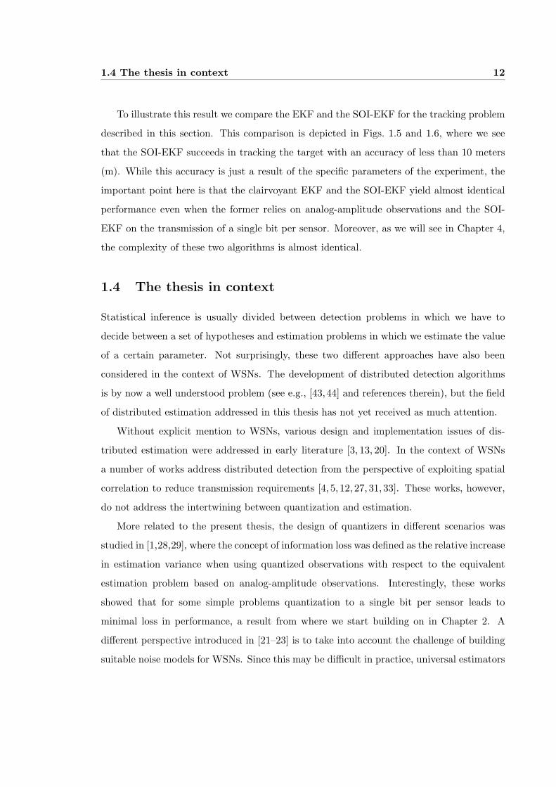
To illustrate this result we compare the EKF and the SOI-EKF for the tracking problem
described in this section. This comparison is depicted in Figs. 1.5 and 1.6, where we see
that the SOI-EKF succeeds in tracking the target with an accuracy of less than 10 meters
(m). While this accuracy is just a result of the specific parameters of the experiment, the
important point here is that the clairvoyant EKF and the SOI-EKF yield almost identical
performance even when the former relies on analog-amplitude observations and the SOI-
EKF on the transmission of a single bit per sensor. Moreover, as we will see in Chapter 4,
the complexity of these two algorithms is almost identical.
1.4 The thesis in context
Statistical inference is usually divided between detection problems in which we have to
decide between a set of hypotheses and estimation problems in which we estimate the value
of a certain parameter. Not surprisingly, these two different approaches have also been
considered in the context of WSNs. The development of distributed detection algorithms
is by now a well understood problem (see e.g., [43,44] and references therein), but the field
of distributed estimation addressed in this thesis has not yet received as much attention.
Without explicit mention to WSNs, various design and implementation issues of dis-
tributed estimation were addressed in early literature [3, 13, 20]. In the context of WSNs
a number of works address distributed detection from the perspective of exploiting spatial
correlation to reduce transmission requirements [4, 5, 12, 27, 31, 33]. These works, however,
do not address the intertwining between quantization and estimation.
More related to the present thesis, the design of quantizers in different scenarios was
studied in [1,28,29], where the concept of information loss was defined as the relative increase
in estimation variance when using quantized observations with respect to the equivalent
estimation problem based on analog-amplitude observations. Interestingly, these works
showed that for some simple problems quantization to a single bit per sensor leads to
minimal loss in performance, a result from where we start building on in Chapter 2. A
different perspective introduced in [21–23] is to take into account the challenge of building
suitable noise models for WSNs. Since this may be difficult in practice, universal estimators

1.4 The thesis in context 13
that work irrespective of the noise distribution were introduced in these works and shown
to have an information loss independent of the network size.
The problem of distributed state estimation of stochastic processes with quantized ob-
servations has received attention in the non-linear filtering community. While the discontin-
uous non-linearity created by quantization precludes application of the extended (E)KF, the
problem can be handled with more powerful techniques such as the unscented (U)KF [15],
or the Particle Filter (PF) [10, 18]. These directions have been pursued in the context of
filtering [8, 45] and target tracking with a WSN [2,11].
Results in the present thesis have appeared in [34–40]. Fundamental properties of the
problem comprising the material covered in Chapter 2 are discussed in [37, 40]. The
pragmatic signal models considered in Chapter 3 and corresponding results appeared
in [34,36,38]. A precursor to the SOI-KF is introduced in [35] whereas the SOI-KF discussed
in Chapter 4 was introduced in [39].
The recent interest in WSNs has led to a number of special issues that are a good starting
point for the uninitiated reader. Fundamental performance limits have been analyzed in [41];
sensor collaboration is argued to be the reason why WSNs can perform complex tasks
even though they consist of inexpensive devices in [19]; and the field of distributed signal
processing for WSNs – the area to which this thesis belongs – is surveyed in [24].

14
Chapter 2
Mean-location in additive white
Gaussian noise
2.1 Introduction
Our focus here in the present chapter is on understanding the fundamental properties of
bandwidth-constrained distributed estimation by looking at the problem of mean-location
parameter estimation in Additive White Gaussian Noise (AWGN). We seek Maximum Like-
lihood Estimators (MLE) and benchmark their variances with the Cramer-Rao Lower Bound
(CRLB) that, at least asymptotically, is achieved by the MLE. We will show that the de-
ciding factor in the choice of the estimator is the Signal Noise Ratio (SNR), defined here as
the dynamic range of the parameter square over the observation noise variance.
Our approach is motivated by the observation that an estimator based on the transmis-
sion of a single binary observation per sensor can have variance as small as π/2 times that
of the clairvoyant sample mean estimator (Section 2.3). This result was derived first in [28]
and is included here as a motivational starting point. By noting that this excellent perfor-
mance can only be achieved under careful design choices, we introduce a class of estimators
that minimize the average variance over a given weight function, establishing that in the
low-to-medium SNR range this class of MLE performs close to the clairvoyant estimator’s
variance (Section 2.3). We then turn our attention to the high SNR regime, and show that

2.2 Problem statement 15
a quantization step close to the noise’s standard deviation is nearly optimal in the sense
of minimizing a properly defined per-bit CRLB (Section 2.5), establishing a second result,
on the optimal number of bits per sensor to be transmitted. The sample mean estimator
based on quantized observations is subsequently analyzed to show that at high SNR even
a simple-minded estimator requires transmission of only a small number of extra bits than
the MLE. This allows us to establish analytically that bandwidth-constrained distributed
estimation is not a relevant problem in high SNR scenarios. For such cases, we advocate
using the sample mean estimator based on the quantized observations for its low complexity
(Section 2.6). The last conclusion of the present chapter is that numerical maximization
required by our MLE can be posed as a convex optimization problem, thus ensuring con-
vergence of e.g., Newton-type iterative algorithms. We finally present numerical results in
Section 2.7
2.2 Problem statement
This chapter considers the problem of estimating a deterministic scalar parameter θ in the
presence of zero-mean AWGN,
x(n) = θ + w(n), n = 0, 1, . . . , N − 1, (2.1)
where w(n) ∼ N (0, σ2), and n is the sensor index. Throughout, we will use p(w) :=
1/(√
2πσ) exp[−w2/(2σ2)] to denote the noise probability density function (pdf).
If all the observations {x(n)}N−1n=0 were available, the MLE of θ would be the Sample
Mean Estimator, x = N−1∑N−1
n=0 x(n). Rightfully, this can be regarded as a clairvoyant
estimator for the bandwidth constrained problem, whose variance is known to be [16, p. 30]
var(x) =σ2
N. (2.2)
Due to bandwidth limitations, however, the observations x(n) have to be quantized and
estimation can only be based on these quantized values. To this end, we will henceforth
think of quantization as the construction of a set of indicator variables (that will be referred

2.3 MLE based on binary observations: common thresholds 16
to, as binary observations)
bk(n) = 1{x(n) ∈ (τk, +∞)}, k ∈ Z, (2.3)
where τk is a threshold defining bk(n), Z denotes the set of integers, and k is used to
index the set of binary observations constructed from the observation x(n). The bandwidth
constraint manifests itself in dictating estimation of θ to be based on the binary observations
{bk(n), k ∈ Z}N−1n=0 . The goal of this chapter is twofold: i) develop the MLE for estimating
θ given a set of binary observations, and ii) study the associated CRLB – a bound that is
achieved by the MLE as N →∞.
Instrumental to the ensuing derivations is the fact that each bk(n) in (2.3) is a Bernoulli
random variable with parameter
qk(θ) := Pr{bk(n) = 1} = F (τk − θ), k ∈ Z, (2.4)
where F (x) := 1/(√
2πσ)∫ +∞x exp(−u2/2σ2)du is the complementary cumulative distribu-
tion function (CDF) of w(n).
The problem under consideration bears similarities and differences with quantization.
On the one hand, for a fixed n the set of binary observations {bk(n), k ∈ Z} specifies
uniquely the quantized value of x(n) to one of the pre-specified levels {τk, k ∈ Z}. On the
other hand, different from quantization in which the goal is to reconstruct x(n) (and the
optimum solution is known to be given by Lloyd’s quantizer [32, p.108]); our goal here is to
estimate θ.
2.3 MLE based on binary observations: common thresholds
Let us consider the most stringent bandwidth constraint, requiring sensors to transmit one
bit per x(n) observation. And as a simple first approach, let every sensor use the same
threshold τc to form
b(n) = 1{x(n) ∈ (τc, +∞)}, n = 0, 1, . . . , N − 1. (2.5)
Dropping the subscript k, we let b := [b(0), . . . , b(N−1)]T , and denote as q(θ) the parameter
of these Bernoulli variables. We are now ready to derive the MLE and the pertinent CRLB.

2.3 MLE based on binary observations: common thresholds 17
Proposition 2.1 [28] The MLE θ based on the vector of binary observations b is given by
θ = τc − F−1
(1N
N−1∑
n=0
b(n)
). (2.6)
Furthermore, the CRLB for any unbiased estimator θ based on b is given by
var(θ) ≥ 1N
[p2(τc − θ)
F (τc − θ)[1− F (τc − θ)]
]−1
:= B(θ). (2.7)
Proof: Due to the noise independence, the pdf of b is p(b, θ) =∏N−1
n=0 [q(θ)]b(n)[1 −q(θ)]1−b(n). Taking logarithm yields the log-likelihood
L(θ) =N−1∑
n=0
b(n) ln(q(θ)) + (1− b(n)) ln(1− q(θ)), (2.8)
whose second derivative with respect to θ is
L(θ) =N−1∑
n=0
b(n)[−p2(τc − θ)
q2(θ)+
p(τc − θ)q(θ)
]+ (2.9)
N−1∑
n=0
[1− b(n)][− p2(τc − θ)
[1− q(θ)]2− p(τc − θ)
1− q(θ)
];
for which we used that ∂q(θ)/∂θ = p(τc−θ), and introduced the definition p(θ) := ∂p(θ)/∂θ.
Since for a Bernoulli variable E[b(n)] = q(θ), the CRLB in (2.7) follows after taking the
negative inverse of E[L(θ)]. The MLE can be found either by maximizing (2.8), or simply
after recalling that the MLE of q(θ) is,
q =1N
N−1∑
n=0
b(n), (2.10)
and using the invariance of MLE [c.f. (2.4) and (2.10)].
Proposition 2.1 asserts that θ can be consistently estimated from a single binary obser-
vation per sensor, with variance as small as B(θ). Minimizing the latter over θ reveals that
Bmin is achieved when τc = θ and is given by
Bmin =2πσ2
4N≈ 1.57
σ2
N. (2.11)

2.3 MLE based on binary observations: common thresholds 18
−2 −1.5 −1 −0.5 0 0.5 1 1.5 20
2
4
6
8
10
12
(τc−θ)/σ
CR
LB
CRLBChernoff bound
Figure 2.1: CRLB and Chernoff bound in (2.13) as a function of the distance between τc
and θ measured in AWGN standard deviation (σ) units.
In words, if we place τc optimally, the variance increases only by a factor of π/2 with respect
to the clairvoyant estimator x that relies on unquantized observations. Using the (tight)
Chernoff bound for the complementary CDF
F (τc − θ)[1− F (τc − θ)] ≤ 14e−
(τc−θ)2
2σ2 , (2.12)
based on which a simple bound on B(θ) can be obtained
B(θ) ≤ πσ2
2Ne+ 1
2[(τc−θ)/σ]2 . (2.13)
Fig. 2.1 depicts B(θ) and its Chernoff bound, from where it becomes apparent that for
|τc−θ|/σ ≤ 1 the increase in variance relative to (2.2) will be around 2 [c.f. (2.7) and (2.13)].
Roughly speaking, to achieve a variance close to var(x) in (2.2), it suffices to place τc
“σ−close” to θ. Fig. 2.2 shows a simulation where we have chosen τc = θ +σ, to verify that
the penalty is, indeed, small.
Accounting for the dependence of var(θ) on τ , σ and the unknown θ, one can envision
an iterative algorithm in which the threshold is iteratively adjusted over time. Call τ(j)c the
threshold used at time j, and θ(j) the corresponding estimate obtained as in (2.6). Having

2.4 MLE based on binary observations: non-identical thresholds 19
60 65 70 75 80 85 90 95 100
0.006
0.008
0.01
0.012
0.014
0.016
0.018
0.02
0.022
N
Var
ianc
e
clairvoyant estimatorCRLBsimulation
Figure 2.2: MLE in (2.6) based on binary observations performs close to the clairvoyant
sample mean estimator when θ is close to the threshold defining the binary observation
(σ = 1, τc = 0, and θ = 1).
this estimate, we can now set τ(j+1)c = θ(j), for subsequent estimates not only benefit from
the increased number of observations but also from improved binary observations. Such an
iterative algorithm fits rather nicely to e.g., a target tracking application.
2.4 MLE based on binary observations: non-identical thresh-
olds
The variance of the estimator introduced in Section 2.3 will be close to var(x) whenever the
actual parameter θ is close to the threshold τ in standard deviation (σ) units. This can be
guaranteed when the possible values of θ are restricted to an interval of size comparable to
σ; or in other words, when the dynamic range of θ is in the order of σ. When the dynamic
range of θ is large relative to σ, we pursue a different approach using binary observations
bk(n), generated from different regions (τk, +∞) in order to assure that there will always
be a threshold τk close to the true parameter. Consider, for each n, the set of binary

2.4 MLE based on binary observations: non-identical thresholds 20
measurements defined by (2.3) and to maintain the bandwidth constraint, let each sensor
transmit only one out of this set of binary observations.
Let Nk be the total number of sensors transmitting binary observations based on the
threshold τk, and define ρk := Nk/N as the corresponding fraction of sensors. We further
suppose that the index kn chosen by sensor n, is known at the destination (the fusion center
or peer sensors in an ad-hoc WSN). Algorithmically, we can summarize our approach in
three steps:
[S1] Define a set of thresholds τ = {τk, k ∈ Z} and associated frequencies ρ = {ρk, k ∈ Z}.
[S2] Assign the index kn to sensor n; i.e., sensor n generates the binary observation bkn(n)
using the threshold τkn . Define b := [bk0(0), . . . , bkN−1(N − 1)]T .
[S3] Transmit the corresponding binary observations to find the MLE as we describe next.
Similar to (2.8), the log-likelihood function is given by
L(θ) =N−1∑
n=0
bkn(n) ln(qkn(θ)) + (1− bkn(n)) ln(1− qkn(θ)), (2.14)
from where we can define the MLE of θ given the {bkn}N−1n=0 ,
θ = arg maxθ{L(θ)}. (2.15)
As θ in (2.15) cannot be found in closed-form, we resort to a numerical search, such as
Newton’s algorithm that is based on the iteration
θ(i+1) = θ(i) − L(θ(i))
L(θ(i)), (2.16)
where L(θ) := ∂L(θ)/∂θ, and L(θ) := ∂2L(θ)/∂θ2 are the first and second derivatives of
the log-likelihood function that we compute explicitly in (2.58) and (2.59) of Appendix
A. Albeit numerically found, the MLE in (2.15) is guaranteed to converge to the global
optimum of L(θ) thanks to the following property:
Proposition 2.2 The MLE problem (2.14) - (2.15) is convex on θ.

2.4 MLE based on binary observations: non-identical thresholds 21
Proof: The Gaussian pdf p(x) is log-concave [6, p. 104]; furthermore, the regions Rk :=
(τk,+∞) and R(c)k are half-lines, and accordingly convex sets. To complete the proof just
note that qk(θ) and 1− qk(θ) are integrals of a log-concave function (p(x)) over convex sets
(Rk and R(c)k respectively); thus, they are log-concave and their logarithms are concave.
Given that summation preserves concavity, we infer that L(θ) is a concave function of θ.
Although numerical MLE problems are typically difficult to solve, due to local minima
requiring complicated search algorithms, this is not the case here. The concavity of L(θ)
guarantees convergence of the Newton iteration (2.16) to the global optimum, regardless of
initialization.
The CRLB for this problem follows from the expected value of L(θ) and is stated in the
following proposition.
Proposition 2.3 The CRLB for any unbiased estimator θ based on b is
B(θ, τ , ρ) =1N
[∑
k
ρkp2(τk − θ)
F (τk − θ)[1− F (τk − θ)]
]−1
:=1N
S−1(θ, τ ,ρ). (2.17)
Proof: See Appendix A.
Since the CRLB in (2.17) depends on the design parameters (τ ,ρ), Proposition 2.3
reveals that using non-identical thresholds across sensors provides an additional degree of
freedom. This is precisely what we were looking for in order to overcome the limitations
of the estimator introduced in Section 2.3. In the ensuing subsection, we will delve on the
selection of (τ , ρ).
2.4.1 Selecting the parameters (τ ,ρ)
Since the CRLB depends also on θ, the selection of (τ , ρ) depends not only on the estimator
variance for a specific value of θ, but also on how confident we are that the actual parameter
will take on this value. To incorporate this confidence we introduce a weighting function,
W (θ), which accounts for the relative importance of different values of θ. For instance, if

2.4 MLE based on binary observations: non-identical thresholds 22
we know a priori that θ ∈ (Θ1,Θ2), we can choose W (θ) = u(θ − Θ1) − u(θ − Θ2), where
u(·) is the unit step function.
Given this weighting function, a reasonable performance indicator is the weighted vari-
ance,
CW :=∫ +∞
−∞W (θ)var(θ) dθ. (2.18)
Although we do not have an expression for the variance of the MLE in (2.15) but only the
CRLB (2.17), we know that the MLE will approach this bound as N →∞. Consequently,
selecting the best possible (τ , ρ) for a prescribed W (θ) amounts to finding the set (τ , ρ)
that minimizes the weighted asymptotic variance given by the weighted CRLB [c.f (2.17)
and (2.18)],
limN→+∞
NCW = NBW (τ , ρ) := N
∫ +∞
−∞W (θ)B(θ, τ , ρ) dθ
=∫ +∞
−∞
W (θ)S(θ, τ ,ρ)
dθ. (2.19)
Thus, the optimum set (τ ∗, ρ∗), should be selected as the solution to the problem
(τ ∗, ρ∗) = arg min(τ ,ρ)
∫ +∞
−∞
W (θ)S(θ, τ ,ρ)
dθ,
s.t.∑
k
ρk = 1, ρk ≥ 0 ∀k. (2.20)
Solving (2.20) is complex, but through a proper relaxation we have been able to obtain the
following insightful theorem.
Theorem 2.1 Assume that∫ +∞−∞ W 1/2(θ) dθ < ∞. Then, the weighted CRLB of any
estimator θ based on binary observations must satisfy,
BW (τ , ρ) ≥ Bmin :=1N
[∫ +∞−∞ W 1/2(θ) dθ
]2
∫ +∞−∞
p2(u)F (u)[1−F (u)] du
(2.21)
Furthermore, the bound is attained if and only if there exist a set (τ , ρ) such that
S(θ, τ , ρ) = KW 1/2(θ), K :=
∫ +∞−∞
p2(u)F (u)[1−F (u)] du
∫ +∞−∞ W 1/2(θ) dθ
. (2.22)

2.4 MLE based on binary observations: non-identical thresholds 23
Proof: See Appendix B.
Note that the claims of Theorem 2.1, are reminiscent of Cramer-Rao’s Theorem in the
sense that (2.21) establishes a bound, and (2.22) offers a condition for this bound to be
attained.
To gain intuition on the performance limit dictated by Theorem 2.1, let us special-
ize (2.21) to a Gaussian-shaped W (θ), with variance σ2θ . In this case, the numerator in (2.21)
becomes, [∫ +∞
−∞W 1/2(θ) dθ
]2
= 2√
2πσθ. (2.23)
The denominator in (2.21) that depends on the noise distribution cannot be integrated in
closed form, but we can resort to the following numerical approximation,∫ +∞
−∞
p2(u)F (u)[1− F (u)]
du ≈ 1.81σ
. (2.24)
Substituting (2.24) and (2.23) in (2.21), we finally obtain
BGGmin ≈ 2.77
σθσ
N= 2.77
σθ
σ
(σ2
N
). (2.25)
Perhaps as we should have expected, the best possible weighted variance for any estimator
based on a single binary observation per sensor can only be close to the clairvoyant variance
in (2.2) when σθ ≈ σ – a condition valid in low to medium SNR scenarios. When the SNR
is high (σθ À σ), the performance gap between (2.2) and (2.25) is significant and a different
approach should be pursued.
A similar derivation leads to an analogous expression for a uniform weight function,
W (θ) = u(θ −Θ1)− u(θ −Θ2),
BGUmin ≈ 0.55
|Θ2 −Θ1|σ
(σ2
N
). (2.26)
Eq. (2.26) similarly allow us to infer that the variance of any estimator based on a single
binary observation per sensor can only be close to the clairvoyant variance in (2.2) when
|Θ2 −Θ1| ≈ σ, which corresponds to a low to medium SNR.
Regarding the achievability of the bound in (2.21), note that although we cannot assure
that there always exists a set (τ , ρ) such that S(θ, τ , ρ) = KW 1/2(θ), we can adopt as a
2.4 MLE based on binary observations: non-identical thresholds 24
relaxed optimal solution the set (τ †, ρ†) that minimizes the distance between S(θ, τ ,ρ) and
KW 1/2(θ)
(τ †, ρ†) =
arg min(τ ,ρ)
∥∥∥∥∥KW 1/2(θ)−∑
k
ρkp2(τk − θ)
F (τk − θ)[1− F (τk − θ)]
∥∥∥∥∥
s.t. ρk > 0. (2.27)
The norm measuring the distance can be any norm in the space of functions. Notwithstand-
ing, we find it convenient to work with the L2 norm.
It is fair to emphasize that (τ †,ρ†) obtained as the solution of (2.27) will in general be
different from the optimum (τ ∗, ρ∗) obtained as the solution of (2.20). Nonetheless (2.27)
offers a more tractable formulation that can be easily solved by methods we outline in
Subsection 2.4.3, and test in Section 2.7. It will turn out that solving (2.27) numerically
yields a small minimum distance, illustrating that the estimator (2.15) based on (τ †, ρ†) is
nearly optimal.
Remark 2.1 The use of a weight function in our deterministic parameter estimation prob-
lem is motivated by maximum a posteriori (MAP) estimation principles which apply to
random parameters. Viewing our deterministic parameter θ as a random one with prior
distribution W (θ), the log-distribution after observing the vector of binary observations is
given by,
LMAP (θ) = L(θ) + ln[W (θ)], (2.28)
with L(θ) given by (2.14). The MAP estimator is defined as θMAP = arg max[LMAP (θ)].
Note that being L(θ) ∝ N , it holds that LMAP (θ) → L(θ) when N → ∞, and ac-
cordingly both estimators coincide asymptotically. In particular, the average variance of
the MAP estimator converges to the average variance of the MLE, and minimization of
BW (τ ,ρ) as defined in (2.19) yields the asymptotically optimum MAP estimator (as well
as the asymptotically optimal MLE).
Also worth mentioning is that if the prior distribution W (θ) is log-concave then the
likelihood in (2.28) is concave. This is the case for many distributions including the Gaussian

2.4 MLE based on binary observations: non-identical thresholds 25
and the Uniform one.
2.4.2 An achievable upper bound on BW (τ ,ρ)
To explore whether we can approach the bound in (2.21), we introduce the following Cher-
noff bound [c.f. (2.12) and (2.17)]
B(θ, τ , ρ) ≤ 1N
[4√2πσ
∑
k
ρkp(τk − θ)
]−1
:=1N
T−1(θ, τ , ρ). (2.29)
Being a superposition of shifted Gaussian bells with variance σ, the bound T (θ, τ , ρ) is
easier to manipulate than S(θ, τ ,ρ) in (2.17). However, the major implication of (2.29) is
that by adjusting the spacing τk−τk−1 := τ = σ, the set of functions G := {p(θ−kτ), k ∈ Z}becomes a Gabor basis [30, Chap. 6]. Therefore, T (θ, τ , ρ) can be thought of as a Gabor
expansion with coefficients ρ, and thus capable of approximating W 1/2(θ) with arbitrary
accuracy.
Theorem 2.2 Define the Gabor basis G := {p(θ − kτ), k ∈ Z} with τ = σ, and consider
the coefficients c = {ck, k ∈ Z} of the Gabor expansion of W 1/2(θ) given by,
c = arg min{ck}
∥∥∥∥∥W 1/2(θ)−∑
k
ckp(kτ − θ)
∥∥∥∥∥ (2.30)
Also, assume that∫ +∞−∞ W 1/2(θ) dθ < ∞. If ck ≥ 0 ∀k, then the weighted CRLB of the
estimator based on the binary observations defined by τ ‡ := {τk = kτ, k ∈ Z}, and ρ‡ :=
{ρk = ck/(∑
k ck), k ∈ Z} is bounded by
BW (τ ‡, ρ‡) ≤ Bmax :=√
2πσ
4N
[∫ +∞
−∞W 1/2(θ) dθ
]2
. (2.31)
Proof: See Appendix B.
Corollary 2.1 If W (θ) is Gaussian-shaped with σθ ≥ σ/√
2 then the weighted CRLB of the
estimator based on binary observations constructed form the set (τ ‡, ρ‡) as in Theorem 2.2
is bounded by,
BW (τ ‡, ρ‡) ≤ Bmax = πσσθ
N. (2.32)

2.4 MLE based on binary observations: non-identical thresholds 26
Proof: The coefficients of the Gabor transform of W 1/2(θ) using the basis G are all posi-
tive [30, Chap. 6]; and the integral of W 1/2(θ) is given by (2.23).
Note that Theorem 2.2 is weaker than Theorem 2.1 in the sense that the former asserts
an upper bound on the asymptotic variance while the latter claims a lower bound. On the
other hand Theorem 2.1 is weaker because it claims the existence of the lower bound, while
Theorem 2.2 claims the achievability of the upper bound.
Perhaps more important is that comparison of (2.32) with (2.25) implies that
Bmax ≈ 1.14Bmin, (2.33)
that is, the gap between the lower and upper bound is small. And, as we wanted to prove,
the solution of (2.27) should give an estimator whose CRLB is close to (within 14%) the
bound Bmin in (2.21).
Even though, it is possible by reducing the distance between thresholds (or using non-
uniform spacings) to further reduce the variance, Theorem 2.2 asserts that this reduction
will be no greater than 14% relative to a uniform spacing with τ = σ. Consequently,
a threshold spacing τ = σ approximates the best performance in (2.25) reasonably well.
Moreover, numerical results in Section 2.7 will justify that a spacing τ ≈ 2σ is good enough
for practical purposes. Note that this result is somewhat counterintuitive since we tend to
think that reducing the distance between thresholds would improve the estimator. However,
the truth is that with a uniform spacing τ = σ (or τ = 2σ as numerical results illustrate)
there is no need for increasing the number of thresholds any further.
2.4.3 Algorithmic Implementation
Theorem 2.1 led to the definition of a near-optimal set (τ †, ρ†) given by the solution of the
infinite-dimensional least-squares problem in (2.27). Furthermore, Theorem 2.2 reinforced
the usefulness of this near-optimal solution as we proved that the CRLB for this (τ †, ρ†)
cannot be very far from the optimal (τ ∗, ρ∗) defined by (2.20). In the present subsection
we will analyze the numerical implementation of (2.27).
A byproduct of Theorem 2.2 is that a uniform threshold spacing τk+1 − τk := τ > σ
captures most of the optimality, and accordingly we begin the numerical implementation by

2.4 MLE based on binary observations: non-identical thresholds 27
defining a threshold spacing τ ≥ σ. This reduces the degrees of freedom by one, simplifying
the numerical implementation to that of finding the set of corresponding frequencies ρk.
The first step is to obtain a finite dimensional problem by discretizing the functions
in (2.27)
ρ∗ = arg minρ
‖s−Pρ‖ (2.34)
s.t. ρ º 0
where s := [S(θ0), . . . , S(θM )]T , ρ := [ρ1, . . . , ρL]T , º denotes element-wise inequality (ρl ≥0 ∀l); M controls the discretization step, L is the number of thresholds whose frequencies
are large enough to be considered of interest; and the matrix P, has entries given by,
[P]ij =p2(τi − θj)
F (τi − θj)[1− F (τi − θj)]. (2.35)
Discretization introduces numerical errors that can be controlled by choosing a small enough
step in the (numerical) evaluation of the integrals. However, this discretization alters the
implicit constraint that∑
k ρk = 1, which was enacted by the normalization constant Kin (2.22). Once the integral is discretized this normalization no longer holds and we have
to make this constraint explicit:
ρ∗ = arg minρ
‖s− Fρ‖ (2.36)
s.t. ρ º 0, ρT1 = 1.
Note that the constrained least squares problem in (2.36) is convex, since the objective is
convex (norms are convex) and the constraints are linear. Moreover, (2.36) can be trans-
formed to a Second Order Cone Program (SOCP) after introducing the auxiliary variable t
to obtain
ρ∗ = arg min(t,ρ)
t (2.37)
s.t. ‖s− Fρ‖ ≤ t, ρ º 0, ρT1 = 1.
It is known that a SOCP can be efficiently solved with standard convex optimization pack-
ages [42]. The implementation of this design is illustrated in Section 2.7 for a pair of different
weighting functions W (θ).

2.5 Relaxing the Bandwidth Constraint 28
2.5 Relaxing the Bandwidth Constraint
The variances of the estimators in Sections 2.3 and 2.4 are close to var(x) either when the
parameter’s range is small, or, in the order of the noise variance. Formally, if for a Gaussian
weight function we define the SNR as γ := σ2θ/σ2, the variance of the estimator in (2.15) is
[c.f. (2.2) and (2.25)]
Bmin = 2.77√
γ var(x). (2.38)
If we let Nsm be the number of observations required by x to achieve the same variance of
the estimator in (2.15) we can see that the number N of binary observations, must increase
by a factor N/Nsm = 2.77√
γ. It is clear that in high-γ scenarios, we need a different
approach motivating the relaxation of the bandwidth constraint pursued in this section.
Specifically, using a sequence of thresholds τ := {τk, k ∈ Z}, we will rely on multiple
binary observations per sensor, b(n) := {bk(n), k ∈ Z}, with corresponding Bernoulli pa-
rameters q := {qk = Pr{x(n) > τk}, k ∈ Z}. Without loss of generality, we will assume that
τk1 < τk2 , when k1 < k2. The entries of b(n) are not independent, since x(n) cannot be at
the same time smaller than τk1 and larger than τk2 for k1 < k2; hence b can only take on
realizations
βl = {βk, k ∈ Z|yk = 1 for k ≤ l, yk = 0 for k > l}. (2.39)
The realization b(n) = βl corresponds to the event {x(n) ∈ (τl, τl+1)}, which re-iterates
our earlier comment that creating multiple binary observations is just a different way of
looking at quantization.
We now express the distribution of b(n) in terms of θ, and from there obtain the per-
sensor log-likelihood as
Ln(θ) =+∞∑
k=−∞δ[βk − b(n)] ln[qk+1(θ)− qk(θ)], (2.40)
where δ[βk−b(n)] := 1 if βk = b(n), and 0 otherwise. Independence across sensors implies,
L(θ) =N−1∑
n=0
Ln(θ), (2.41)

2.5 Relaxing the Bandwidth Constraint 29
0.5 1 1.5 2 2.5 31
1.2
1.4
1.6
1.8
2
threshold spacing (τ/σ)
CR
LB /
var sm
Variance as a function of threshold spacing
MLE − worst caseMLE − best caseQSME
−2 −1.5 −1 −0.5 0 0.5 1 1.5 21
1.2
1.4
1.6
1.8
2
θ/σ
CR
LB(θ
)
Variance for different threshold spacings
τ/σ = 1τ/σ = 2τ/σ = 3
Figure 2.3: Variance of the estimator relying on the whole sequence of binary observations.
The room for improved performance once τ < σ is small.
and yields the MLE of θ given {b(n)}N−1n=0 as
θ = arg maxθ{L(θ)}. (2.42)
Two important features of θ in (2.42) are summarized next.
Proposition 2.4 :
(a) The log-likelihood (2.41) is a concave function of θ.
(b) The CRLB of any unbiased estimator of θ based on {b(n)}N−1n=0 is given by
B(θ) =1N
[+∞∑
k=−∞
[p(τk+1 − θ)− p(τk − θ)]2
F (τk+1 − θ)− F (τk − θ)
]−1
. (2.43)
Proof: See Appendix C.
The concavity of L(θ) in (2.41) asserted by Proposition 2.4-(a) implies existence of a
reliable numerical implementation of θ in (2.42). To understand Proposition 2.4-(b) notice
that for an infinite set of equally spaced thresholds (with spacing τ := τk+1 − τk), B(θ)
2.5 Relaxing the Bandwidth Constraint 30
in (2.43) is periodic with period τ . Fig. 2.3 depicts B(θ) parameterized by τ/σ, along with
the maximum and minimum values of B(θ) as functions of τ/σ. Note that for a given τ
the worst and best variances are almost equal for τ ≤ 2σ, being for all practical purposes
constant when τ ≤ σ. More important, when τ ≤ σ, B(θ) is almost equal to the clairvoyant
estimator’s variance.
We now turn our attention to designing a transmission scheme for the infinite number
of binary observations per sensor. This can be done by noting that if bk(n) = 1, then
bk′(n) = 1 for k′ < k; and likewise if bk(n) = 0, then bk′(n) = 0 for k′ > k. Accordingly,
each binary observation transmitted provides information about half of the thresholds, and
the required number of bits Nt to be transmitted per sensor grows logarithmically with the
allowable parameter range. The actual value of Nt will depend on the parameter’s range;
e.g., for θ ∈ [−U,U ] it will be Nt ≈ log2[(σ + 2U)/τ ]. When the prior knowledge about θ
dictates a Gaussian prior W (θ) the result can be summarized in the following proposition.
Proposition 2.5 When W (θ) is a Gaussian bell with variance σ2θ , the infinite set of binary
observations b(n) can be transmitted using Nt bits satisfying
E(Nt) < 3 +[log2 Q−1(1/4) +
12
log2
(σ2
θ + σ2
τ2
)]
+
, (2.44)
where τ := τk+1 − τk ∀k, Q(x) := 1/(√
2π)∫ +∞x exp(−u2/2) du, and [x]+ := max(0, x).
Proof: See Appendix D.
Combining Propositions 2.4-(b) and 2.5 yields a benchmark on the performance of es-
timators based on binary observations. For a given bandwidth constraint, we determine τ
from (2.44), and from there the benchmark variance from (2.43).
Note that (2.44) can also be written using a slightly more intuitive expression in terms
of γ
E(Nt) < 2.43 +12
log2 (1 + γ) + log2
(σ
τ
), (2.45)
where we substituted the constants in (2.44) by their explicit values, and assumed for
simplicity that the argument inside the [·]+ operator is positive (valid if τ2 < 0.45(σ2θ +σ2)).
The first logarithmic term in (2.45) can be viewed as quantifying the information that each

2.5 Relaxing the Bandwidth Constraint 31
observation x(n) carries about the underlying parameter, while the second logarithmic
term can be thought of as quantifying our confidence on the observations. By decreasing
τ beyond σ we are adding bits to the quantization of x(n) reflecting our belief that there
is more information to be extracted from it. In the next section, we will see that it makes
sense to set τ = σ, in which case Nt reduces to
E(Nt) < 2.43 +12
log2 (1 + γ) . (2.46)
Eq. (2.46) is valid, when γ ≥ 1.20, in which case it is a tight bound in the expected value of
transmitted bits. When γ < 1.20, the bound reduces to E(Nt) < 3 which is too loose to be
of practical interest. However, remember that for this low SNR scenario we advocate the
estimator introduced in Section 2.4 and this limitation of (2.46) is not a concern.
2.5.1 Optimum threshold spacing
Estimation problems are usually posed for a given number of measurements; but for
bandwidth-constrained problems, a more meaningful formulation is to prescribe the to-
tal number of available bits, Nb. That is, given the channel (bandwidth, SNR, and time)
we are allowed to transmit up to Nb bits that have to be allocated among the observations.
Fine quantization implies a small per-observation variance, but also a small number of ob-
servations N ; while coarse quantization increases the variance per-observation but allows
for a larger N .
A convenient metric for a bandwidth-constrained estimation problem is the following:
Definition 2.1 Suppose that for a given estimator based on binary observations, the trans-
mission of binary observations requires an average of Nt bits. Define the per-bit worst case
CRLB as:
Cb = Nt maxθ{B(θ)}. (2.47)
For a bandwidth constraint Nb, the variance will be bounded by var(θ) ≥ Cb/Nb.
Applying Definition 2.1 to the CRLB in (2.43), we deduce that Cb is a function of the
spacing τ
Cb(τ) = Nt(τ)maxθ{B(θ, τ)}, (2.48)
2.6 Quantized sample mean estimator 32
what raises the question about the existence of an optimum threshold spacing τ∗(γ)
τ∗ = arg minτ{Cb(τ)}. (2.49)
For this question to be meaningful, τ∗ should be neither zero nor infinity, which is true for
the problem considered in the current section.
Proposition 2.6 For a Gaussian shaped W (θ), the optimum threshold spacing τ∗ in (2.49)
is finite and different from zero.
Proof: When τ → 0, Cb(τ) → +∞ because Nt → +∞ while B(θ) is bounded; furthermore
when τ → +∞, Cb(τ) → +∞ because B(θ) → +∞ faster that Nt → 0 (exponentially versus
logarithmically). As Cb(τ) is continuous and approaches ∞ in both extremes, it must have
a minimum.
By taking into account the bandwidth constraint we proved the existence of an optimum
quantization step τ∗ that minimizes Cb for a given γ; and a corresponding optimum number
of bits per observation. Fig. 2.4 depicts τ∗(γ). It is apparent from these curves, that the
optimum value is quite insensitive to variations of γ. When γ varies from 0 dB to 50 dB
(a 105 range) τ∗ moves from 2σ to σ. Furthermore, the curves Cb(τ) are very flat around
the optimum, implying that we can adopt τ = σ as a working compromise for the optimum
threshold spacing (i.e., quantization step).
2.6 Quantized sample mean estimator
It is interesting to compare the MLE estimator in (2.42) with the low complexity quantized
sample mean estimator (QSME). Consider the observations {x(n)}N−1n=0 and quantize them
with a uniform quantizer at resolution τ to obtain
xQ(n) = τ round[x(n)/τ ], (2.50)
where xQ denotes the quantized observations and round(x) is the integer closest to x.
The QSME is just the sample mean of the quantized observations
xQ(n) :=1N
N−1∑
n=0
xQ(n), (2.51)
2.6 Quantized sample mean estimator 33
0 5 10 15 20 25 30 35 40 45 500.5
1
1.5
2
2.5
SNR (γ = σθ2/σ2)
Opt
imum
spa
cing
(τ* )
Optimum threshold spacing as a function of SNR
0 0.5 1 1.5 2 2.5 30
5
10
15
20
25
threshold spacing (τ/σ)
Cb
Worst case per bit CRLB as a function of τ
γ = 5dbγ = 25dbγ = 50 db
Figure 2.4: Variation of the threshold spacing that minimizes the worst case per bit CRLB
with the SNR. Cb(τ) is very flat around the optimum and τ∗ has a small change when the
SNR moves over a range of 50 dB.
which is a desirable estimator if one just ignores the bandwidth constraint. Interestingly,
this simple estimator is not very far from the MLE in (2.42) as stated in the following
proposition.
Proposition 2.7 The variance of the QSME in (2.51) is bounded by
E[(xQ − θ)2] ≤(
1 +τ
σ+
τ2
4σ2
)σ2
N. (2.52)
Proof: See Appendix E.
Note that since xQ is biased, the pertinent performance metric is the Mean Square Error
(MSE), not the variance. Fig. 2.3 shows that the MSE of the MLE for a threshold spacing
τ = 2σ is roughly comparable to the MSE of the QSME for a spacing τ = σ/2.
For low SNR problems in which the cost of each sequence of binary observations is just
a few bits, adding two more bits in order to use the QSME offers a rather poor solution.
Meanwhile, when the SNR is high, the addition of two bits to a long sequence carries a
small relative increase in the bandwidth requirement. While the break point depends on

2.7 Numerical results 34
the desired complexity-performance tradeoff, it is clear that when the SNR is high the
bandwidth-constrained estimation problem is of little interest since even a “simple-minded”
estimator performs close to the optimum MLE in (2.42). The effort in finding efficient
bandwidth-constrained distributed estimation algorithms should, thus, be focused on low
SNR scenarios.
2.7 Numerical results
We implement here the estimator introduced in Section 2.4, for which there are two aspects
we want to study; the design of (τ , ρ) by numerically solving (2.37); and the implementation
of the estimator itself. Recall that with thresholds spaced by less than σ, the room for
increasing performance is limited, and thus we are also interested in studying the effect the
spacing τ has on the average estimation variance.
2.7.1 Designing (τ , ρ)
For a given threshold spacing τ , the set of frequencies ρ is obtained as the solution of the
SOCP in (2.37). Figs. 2.5 and 2.6 show the result of computing ρ for the case of Gaussian
and Uniform weighting functions, respectively. In both cases, it is apparent that a threshold
spacing τ = 2σ suffices to achieve a small MSE.
This is even more clear in the uniform case where reducing the spacing results in nulling
some of the ρk. Particularly interesting are the error curves depicting the difference between
W 1/2(θ) and S(θ, τ ,ρ). When the threshold spacing is reduced from τ = 2σ to τ = σ the
error is almost unchanged. Although we have not established this analytically, it appears
that choosing the thresholds with a spacing smaller than 2σ is of no practical value.
2.7.2 Estimation with 1 bit per sensor
The estimation problem itself is solved using Newton’s algorithm based on the itera-
tion (2.16). The results are shown on Fig. 2.7 for a Gaussian weight function with 2σ
spacing between thresholds. For each value of N the experiment is repeated 200 times, and

2.7 Numerical results 35
−5 0 50
0.05
0.1
0.15
τ = 3 σ
θ
[W(θ
)]1/
2
[W(θ)]1/2
S(θ)
−5 0 50
0.05
0.1
0.15
τ = σ
θ
[W(θ
)]1/
2
[W(θ)]1/2
S(θ)
−5 0 5−2
−1
0
1
2Relative error for τ = 2σ and τ=σ
θ
Rel
ativ
e er
ror
(%)
τ=στ=2σ
−5 0 50
0.05
0.1
0.15
Frequencies (ρk) for the case τ=σ
ρP
ρ(ρ)
Figure 2.5: Gaussian noise and Gaussian-shaped weight function. Although a threshold
spacing τ = σ reduces the approximation error to almost zero, a spacing τ = 2σ is good
enough in practice (σ = 1, and σθ = 2).
−10 −5 0 5 100
0.02
0.04
0.06
0.08
0.1τ = 3 σ
θ
[W(θ
)]1/
2
[W(θ)]1/2
S(θ)
−10 −5 0 5 100
0.02
0.04
0.06
0.08
0.1τ = σ
θ
[W(θ
)]1/
2
[W(θ)]1/2
S(θ)
−6 −4 −2 0 2 4 6−6
−4
−2
0
2
4
6Relative error for τ = 2σ and τ=σ
θ
Rel
ativ
e er
ror
(%)
τ=στ=2σ
−10 −5 0 5 100
0.05
0.1
0.15
Frequemcies (ρk) for the case τ=σ
ρ
Pρ(ρ
)
Figure 2.6: Gaussian noise and Uniform weight function. A threshold spacing τ = σ has
smaller MSE but a spacing τ = 2σ is better in most of the non-zero probability interval
(σ = 1, and prior U[-7,7]).

2.7 Numerical results 36
100 200 300 400 500 600 700 8000
0.01
0.02
0.03
0.04
0.05
0.06
0.07
0.08
0.09Weighted variance for Gaussian noise and Gaussian prior
Wei
ghte
d va
rianc
e
Number of observations
empirical weighted variancetheoretical weighted variance
Figure 2.7: Gaussian noise and Gaussian weight function. With a threshold spacing τ = 2σ
we achieve a good approximation to the minimum asymptotic average variance (σ = 1,
τ = 2, and σθ = 2).
the average variance is plotted against the theoretical threshold which reasonably predicts
its value. This also reinforces the observation that a threshold spacing τ = 2σ, is good
enough for practical purposes.
2.7.3 Comparison with deterministic control signals
The exponential increase of the CRLB in (2.7) was first observed in [28]. In particular, if
θ ∈ [−Θ,Θ], and we define ∆ = Θ/σ the worst case CRLB is [c.f. (2.7) with τc = 0],
Bmax =2πσ2
NQ(∆)[1−Q(∆)]e∆2
; (2.53)
whose growth is approximately exponential in ∆; which can be interpreted as the parameter
range measured in standard deviation units.
As noted before, while this is satisfactory for ∆ ≈ 1, a different approach is needed
for ∆ > 1. To alleviate this problem, adding control signals to the original observations
was advocated by [28]. Though different classes of control signals were proposed in [28],

2.7 Numerical results 37
102
10−2
10−1
Average variance for Gaussian noise and Gaussian prior
Ave
rage
var
ianc
e
Number of sensors / observations
Optimized thresholds − theoretic boundOptimized thresholds − empiricalEqual frequency thresholds − empirical
Figure 2.8: The average variance of the optimum set (τ ,ρ) found as the solution of (2.37),
yields a noticeable advantage over the use of equispaced equal frequency thresholds as
defined by (2.55) (σ = 1, τ = 2, and σθ = 2).
particularly related to the present work are deterministic control signals of the form,
x(n) = θ + w(n) + s(n), (2.54)
where s(n) is a known periodic waveform, chosen as to minimize the worst case CRLB in
[−Θ, Θ]. To this end it suffices to use a K-periodic sawtooth waveform s(n) = 2Θ/(K −1)[−(K − 1)/2 + n mod K] with appropriately chosen period K.
Such control signals can be seen to be equivalent to the use of multiple equispaced
thresholds with equal frequency,
τk =2Θ
K − 1k, ρk =
1K
, (2.55)
for k = 1, . . . , K. It can be shown that for large enough Θ, the maximum CRLB is minimized
by the (min-max optimum) threshold spacing τk − τk−1 = 2.59σ.
The difference with the approach in Section 2.4 is, of course, that the thresholds are
optimized after averaging over a certain weight function.

2.7 Numerical results 38
To illustrate a case where our approach could be of interest consider a parameter θ ∈(−∞,∞) and a Gaussian weight function with variance σθ. While in this case the range
is not limited we can consider for practical purposes that θ ∈ [−3σθ, 3σθ] and compare the
performance of the estimator defined by the set (τ , ρ) given in (2.55), with the optimum
set (τ , ρ) found as the solution of (2.37). An example comparison is depicted in Fig. 2.8
from where we observe a noticeable difference favoring the second approach.
This difference is just a manifestation of optimization options, with each option being
applicable in different situations.
2.8 Appendices 39
2.8 Appendices
2.8.1 Proof of Proposition 2.3
Let us first note that from the form of L(θ) in (2.14), the MLE estimators of qk
qk =1
Nk
N−1∑
n=0
bknδ(knk− k), (2.56)
are sufficient statistics for this problem, and, (2.14) reduces to
L(θ) =∑
k
Nkqk ln(qk(θ)) + Nk(1− qk) ln(1− qk(θ)), (2.57)
from where we can obtain the first
L(θ) =∑
k
Nkqkp(τk − θ)F (τk − θ)
−Nk(1− qk)p(τk − θ)
1− F (τk − θ), (2.58)
and second derivative
L(θ) =∑
k
Nkqk
[− p2(τk − θ)
F 2(τk − θ)+
p(τk − θ)F (τk − θ)
]− (2.59)
Nk(1− qk)[
p2(τk − θ)[1− F (τk − θ)]2
+p(τk − θ)
1− F (τk − θ)
]
required by Newton’s iteration in (2.16). In deriving (2.58) and (2.59) we used that
qk(θ) = F (τk − θ), and ∂qk(θ)/∂θ = p(τk − θ). As we defined before, p(u) := ∂p(u)/∂u =
−(u/σ2)p(u).
To obtain the CRLB, we simply take the expected value of (2.59) with respect to b.
Since qk is unbiased (E(qk) = qk), the terms involving p(τk−θ) disappear and (2.17) follows.
2.8.2 Proof of Theorems 2.1 and 2.2
We begin by introducing a lemma required by the proofs of both theorems.
Lemma 2.1 If∫ +∞−∞ W 1/2(θ) dθ < ∞ the solution of the variational problem
arg minS F(S) :=∫ +∞
−∞
W (θ)S(θ)
dθ
s.t.∫ +∞
−∞S(θ) dθ = I, (2.60)

2.8 Appendices 40
is given by the function,
S∗(θ) =I∫ +∞
−∞ W 1/2(θ)W 1/2(θ) . (2.61)
The corresponding minimum value is given by
F(S∗) =
[∫ +∞−∞ W 1/2(θ) dθ
]2
I . (2.62)
Proof: Introducing a multiplier λ and considering a variation δS(θ) we obtain
δF =∫ +∞
−∞
[−W (θ)S2(θ)
− λ
]δS(θ) dθ, (2.63)
which after setting the variation to zero yields
S(θ) =−1λ
[W (θ)]12 . (2.64)
The latter is equivalent to (2.61), and the multiplier λ can be obtained from the constraint
as
− 1λ
=I∫ +∞
−∞ [W (θ)]12
. (2.65)
The optimum value of the functional is found after substituting (2.64) into F(S) to
yield (2.62).
Theorem 2.1
Notice that S(θ, τ , ρ), considered as a function of θ, cannot vary over the whole space of
functions, but over a restricted class dictated by (2.17), subject to the constraint∑
k ρk = 1.
Minimizing (2.20) is complex, but as pointed out before it can be relaxed to a simpler
problem by translating the constraint over ρ into a constraint over S(θ, τ ,ρ). To this end,
consider ∫ +∞
−∞S(θ, τ , ρ)dθ =
∫ +∞
−∞
∑
k
ρkp2(τk − θ)
F (τk − θ)[1− F (τk − θ)]dθ, (2.66)
and interchange summation with integration to obtain∫ +∞
−∞S(θ, τ , ρ)dθ =
∑
k
ρk
∫ +∞
−∞
p2(τk − θ)F (τk − θ)[1− F (τk − θ)]
dθ. (2.67)

2.8 Appendices 41
But now, note that the integrals inside the summation are all equal since they contain
shifted versions of the same function. Moreover, recalling that∑
k ρk = 1, we obtain∫ +∞
−∞S(θ, τ , ρ) dθ =
∫ +∞
−∞
p2(u)F (u)[1− F (u)]
du := I1. (2.68)
Thus, we can relax (2.20) to
arg minS
1N
∫ +∞
−∞
W (θ)S(θ)
dθ,
s.t.∫ +∞
−∞S(θ) dθ = I1 . (2.69)
It is important to stress that (2.20) and (2.69) are not equivalent because the func-
tions {S(θ, τ , ρ)} subject to∑
k ρk = 1 are a subset of the functions {S(θ)} subject to∫ +∞−∞ S(θ) dθ = I1. However, the very condition of being a subset dictates that the solution
of (2.69) is a lower bound on the solution of (2.20).
Invoking Lemma 2.1 to solve the variational problem in (2.69), we obtain the
bound (2.21), and requiring S(θ, τ ,ρ) = S∗(θ) renders the condition for this bound achiev-
able.
Theorem 2.2
Starting from (2.29) we can rephrase the problem of finding the optimum set (τ , ρ), as
that of finding the set that minimizes the average of the bound (2.29) over the weighting
function W (θ),
BW (τ , ρ) ≤ 1N
∫ +∞
−∞
W (θ)T (θ, τ ,ρ)
dθ. (2.70)
As before, we relax the problem to the minimization of a functional F(T ) subject to a
constraint on the integral of T (θ, τ , ρ),∫ +∞
−∞T (θ, τ , ρ)dθ =
∫ +∞
−∞
4√2πσ
∑
k
ρkp(τk − θ)dθ =4√2πσ
. (2.71)
By Lemma 2.1, the minimum bound is achieved when
T ∗(θ) =4√2πσ
W 1/2(θ)∫ +∞−∞ W 1/2(θ) dθ
, (2.72)

2.8 Appendices 42
and the function that achieves this minimum is
F(T ∗) =√
2πσ
4
[∫ +∞
−∞W 1/2(θ) dθ
]2
. (2.73)
Finally, and this time different from the proof of Theorem 2.1, we can go a step forward.
According to the hypothesis, the coefficients c = {ck, k ∈ Z} of the Gabor expansion
of W 1/2(θ) over the basis G := {p(θ − kτ), k ∈ Z} are all positive. Thus, by setting
τ ‡ := {τk = kτ, k ∈ Z}, and ρ‡ := {ρk = ck/(∑
k ck), k ∈ Z} we have that
T ∗(θ) = T (θ, τ ‡, ρ‡) . (2.74)
QED.
2.8.3 Proof of Proposition 2.4
To compute the CRLB, recall that qk(θ) = F (τk − θ) and differentiate (2.40) to obtain
∂Ln(θ)∂θ
=+∞∑
k=−∞δ[yk−b(n)]
[[p(τk+1− θ)−p(τk− θ)]2
[F (τk+1− θ)−F (τk− θ)]2(2.75)
− [p(τk+1− θ)− p(τk− θ)]F (τk+1− θ)− F (τk− θ)
]
where p(u) := ∂p(u)/∂u. On the other hand, note that
E[δ(yk − b(n))] = F (τk+1 − θ)− F (τk − θ) . (2.76)
Averaging (2.75), yields the per-observation CRLB,
[Bn(θ)]−1 =+∞∑
k=−∞
[p(τk+1 − θ)− p(τk − θ)]2
F (τk+1 − θ)− F (τk − θ)(2.77)
−+∞∑
k=−∞[p(τk+1 − θ)− p(τk − θ)] .
Finally, note that the second summation is equal to zero from where (2.43) follows readily.
To prove that Ln(θ) is concave, note that we can write,
[qk+1(θ)− qk(θ)] =∫ τk+1−θ
τk−θp(u)du =
∫
(τk,τk+1)p(u− θ)du. (2.78)
Since [qk+1(θ)− qk(θ)] is the integral of a log-concave function (p(u)) over a convex region
(the segment (τk, τk+1)) it is log-concave. Ln(θ) is concave because it is a weighted sum of
logarithms of log-concave functions.

2.8 Appendices 43
2.8.4 Proof of Proposition 2.5
We start by proving a property of the Gaussian Complementary CDF, stated in the following
lemma.
Lemma 2.2 If the positive argument function f(u) : R+ → R, solves
F (u) = 2F (u + f(u)), (2.79)
then, f(u) < f(0), ∀u > 0 .
Proof: Note that f(u) > 0, and take derivatives in both sides of (2.79) to obtain the
derivative of f(u),
f(u) :=df(u)du
=12e−
f(u)[f(u)−2u]
2σ2 − 1. (2.80)
Now note that f(0) = F−1(1/4) ≈ 0.67σ, and consequently f(0) ≈ −0.37 < 0 implying
that f(u) is decreasing around 0. Supposing that f(0) is reached at other values, let v > 0
denote the smallest real number such that f(v) = f(0). From (2.80) we see that f(u) is
decreasing in u; so it must be that f(v) < f(u) < 0, implying that f(v) is decreasing around
v. This is a contradiction since f(u) is continuous.
To prove Proposition 2.5. we introduce a transmission scheme requiring the number of
bits given by (2.44). Begin by noting that the unconditional distribution of x(n) is Gaussian
x(n) ∼ N (µ, σx) ∼ N(
µ,√
σ2θ + σ2
), (2.81)
and assume without loss of generality that µ = 0.
Given (2.81), construct the sequence Γ = {γj}∞k=0 whose elements satisfy
Pr{x(n) > γj} = 2−(j+1). (2.82)
That is, γ0 is the median of the distribution (i.e., γ0 = µ = 0), γ1 is such that (1/4)th of
the probability lies to its right, γ2 such that (1/8)th, and so on.
Remark 2.2 Application of Lemma 2.2 to the definition of Γ allows us to conclude that
γk − γk−1 ≤ γ1.

2.8 Appendices 44
We point two consequences of the definition of the sequence Γ: first, the probability
that x(n) lies between γj−1 and γj given that x(n) > 0 is,
Pr{γj−1 < x(n) < γj} = 2−j ; (2.83)
and second in any given interval (γj , γj + 1) the number N(γj) of equally spaced thresholds
τk is bounded by
N(γj) <
⌈γj − γj−1
τ
⌉. (2.84)
We can now introduce the transmission scheme as follows:
[S1] If x(n) ≥ 0 then transmit 1; and if x(n) < 0 transmit 0 and change the sign of x(n);
[S2] Transmit 1 if x(n) > γj , and 0 otherwise. Start this process at j = 1, and repeat it
until the first j for which x(n) < γj . This confines x(n) to the interval (γj−1, γj) that
contains a total number of N(γj) thresholds bounded by (2.84).
[S3] Enumerate the binary observations bk(n) over the interval (γj−1, γj) from 1 to N(γj)
and transmit them as follows:
[S3a] Set K = dN(γj)/2e, and transmit bK(n)
[S3b] Set K = dK + K/2e if bK(n) = 1, or K = dK −K/2e if bK(n) = 0;
[S3c] Repeat [S3a]-[S3b] until τK − x(n) < τ .
Despite the involved description, the scheme is actually very simple. In steps [S1] and [S2]
we divide the line in segments so that the probability of finding x(n) in any of them is 1/2
the probability of finding it in the previous one. After this is completed, we switch back to
the binary observations and transmit them using pretty much the same scheme. We start
with the binary observation that lies (approximately) in the middle of the interval, and
then depending on the value of the binary observation we transmit the observation closest
to the first quarter or the third quarter and so on.
Although not strictly needed for the proof we elaborate on two issues. On the one hand,
note that the thresholds γj are not being used to define binary observations, but instead
to transmit the observations defined by the thresholds τk. On the other hand, observe

2.8 Appendices 45
that the rationale for steps [S3a]-[S3c] is that over the interval (γj−1, γj) the pdf of x(n)
is more or less constant; i.e., x(n) is approximately uniformly distributed when the event
{x(n) ∈ (γj−1, γj)} is given. This justifies the way the transmission is designed since we
expect the probabilities of finding x(n) to the right or the left of the middle threshold τK
to be equal once we know that x(n) ∈ (γj−1, γj).
Now, we compute the expected value of the transmitted number of bits. First, note that
the number of bits required in steps [S3a]-[S3c] can be bounded using (2.84)
l(1)j = dlog2(N(γj)− 1e+ <
[log2
γj+1 − γj
τ
]
+
, (2.85)
where the −1 comes from the stopping criterion (the last binary observation does not need
to be transmitted), and the + subscripts are because l(1)j cannot be negative.
Second, note that if x(n) ∈ (γj−1, γj), then transmitting the sequence Γ requires
l(2)j = j + 1 (2.86)
bits. Combining the number of bits required when x(n) ∈ (γj−1, γj) given by (2.85)
and (2.86), with the probability that x(n) belongs to this interval, we find the expected
value of Nt as
E(Nt) =+∞∑
j=1
(l(1)j + l
(2)j )2−j (2.87)
<
+∞∑
j=1
[(log2
γj+1 − γj
τ
)
+
+ j + 1]
12j
.
To complete the proof, invoke Remark 2 and note that γ1 = F−1[1/4] = σxQ−1[1/4] to
reduce (2.87) to
E(Nt) <+∞∑
j=1
12j
[1 +
(log2 Q−1[1/4]
σx
τ
)+
]+
+∞∑
j=1
j
2j. (2.88)
Substituting the values of the geometric series (∑+∞
j=1 2−j = 1 and∑+∞
j=1 j2−j = 2), and
remembering that σx =√
σ2θ + σ2, (2.44) follows.

2.8 Appendices 46
2.8.5 Proof of Proposition 2.7
Let b(θ) denote the bias of the QSME,
b(θ) := E(xQ − θ) = E(xQ − x), (2.89)
where the second equality follows from the unbiasedness of x. We can write the MSE in
terms of the bias
E[(xQ − θ)2] = E[(xQ − θ − b(θ))2] + b2(θ) (2.90)
= E[( (xQ − x− b(θ)) − (θ − x) )2] + b2(θ)
where in the second equality we added and subtracted x. The important point is that based
on (2.89) the two variables (xQ − x− b(θ)) and (θ− x) are zero-mean; hence, we can apply
the triangle inequality
E[(xQ − θ)2] ≤ E[(xQ − x− b(θ))2] + b2(θ) + E[(θ − x)2]
+ 2√
E[(xQ − x− b(θ))2]E[(θ − x)2]
≤ E[(xQ − x)2] + E[(θ − x)2]
+ 2√
E[(xQ − x− b(θ))2]E[(θ − x)2]
= E[(xQ − x)2] + var(x)
+ 2√
E[(xQ − x− b(θ))2]var(x). (2.91)
Finally, note that since the quantization error is absolutely bounded by τ/2 we have
E[(xQ − x− b(θ))2] ≤ E[(xQ − x)2]
=1
N2
N−1∑
n=0
E[(x(n)− xQ(n))2]
≤ τ2
4N. (2.92)
Substituting (2.92) and (2.2) into (2.91), we obtain,
E[(xQ − θ)2] ≤ σ2
N+
τ2
4N+ 2
√σ2
N
τ2
4N, (2.93)
which after simplifying establishes (2.52).

47
Chapter 3
Distributed batch estimation based
on binary observations
3.1 Introduction
In the previous chapter we studied estimation of a scalar mean-location parameter in the
presence of zero-mean additive white Gaussian noise. For this simple model, we define the
so called quantization signal-to-noise ratio (Q-SNR) as the ratio of the parameter’s dynamic
range over the noise standard deviation, and advocated different strategies depending on
whether the Q-SNR is low, medium or high. An interesting conclusion from Chapter 2 is
that in low-medium Q-SNR, estimation based on sign quantization of the original observa-
tions exhibits variance almost equal to the variance of the (clairvoyant) estimator based on
unquantized observations. Interestingly, for the pragmatic class of models considered here it
is still true that transmitting a few bits (or even a single bit) per sensor can approach under
realistic conditions the performance of the estimator based on unquantized data. The
impact of the latter to WSNs is twofold. On the one hand, we effect energy savings by
transmitting a single bit per sensor; and on the other hand, we simplify analog to digital
conversion to (inexpensive) signal level comparation. While results in the present chapter
apply only when the Q-SNR is low-to-medium this is rather typical for WSNs.
We begin with mean-location parameter estimation in the presence of known univariate
3.2 Problem Statement 48
but generally non-Gaussian noise pdfs (Section 3.3.1). We next develop mean-location pa-
rameter estimators based on binary observations and benchmark their performance when
the noise variance is unknown; however, the same approach in principle applies to any noise
pdf that is known except for a finite number of unknown parameters (Section 3.3.2). Sub-
sequently, we move to the most challenging case where the noise pdf is completely unknown
(Section 3.4). Finally, we consider vector generalizations where each sensor observes a given
(possibly nonlinear) function of the unknown parameter vector in the presence of multivari-
ate and possibly colored noise (Section 3.5). While challenging in general, it will turn out
that under relaxed conditions, the resultant Maximum Likelihood Estimator (MLE) is the
maximum of a concave function, thus ensuring convergence of Newton-type iterative al-
gorithms. Moreover, in the presence of colored Gaussian noise, we show that judiciously
quantizing each sensor’s data renders the estimators’ variance stunningly close to the vari-
ance of the clairvoyant estimator that is based on the unquantized observations; thus, nicely
generalizing the results of Sections 3.3.1, 3.3.2, and Chapter 2 to the more realistic vector
parameter estimation problem (Section 3.5.1). Numerical examples corroborate our theo-
retical findings in Section 3.6, where we also test them on a motivating application involving
distributed parameter estimation with a WSN for measuring vector flow (Section 3.6.2).
3.2 Problem Statement
Consider a WSN consisting of N sensors deployed to estimate a deterministic p× 1 vector
parameter θ. The nth sensor observes an M × 1 vector of noisy observations
x(n) = fn(θ) + w(n), n = 0, 1, . . . , N − 1 , (3.1)
where fn : Rp → RM is a known (generally nonlinear) function and w(n) denotes zero-mean
noise with pdf pw(w), that is either unknown or known possibly up to a finite number of
unknown parameters. We further assume that w(n1) is independent of w(n2) for n1 6= n2;
i.e., noise variables are independent across sensors. We will use Jn to denote the Jacobian
of the differentiable function fn whose (i, j)th entry is given by [Jn]ij = ∂[fn]i/∂[θ]j .
Due to bandwidth limitations, the observations x(n) have to be quantized and estimation

3.3 Scalar parameter estimation – Parametric Approach 49
of θ can only be based on these quantized values. We will henceforth think of quantization
as the construction of a set of indicator variables
bk(n) = 1{x(n) ∈ Bk(n)}, k = 1, . . . , K , (3.2)
taking the value 1 when x(n) belongs to the region Bk(n) ⊂ RM , and 0 otherwise.
Throughout, we suppose that the regions Bk(n) are computed at the fusion center where
resources are not at a premium.
Estimation of θ will rely on the set of binary variables {bk(n), k = 1, . . . , K}N−1n=0 . The
latter are Bernoulli distributed with parameters qk(n) satisfying
qk(n) := Pr{bk(n) = 1} = Pr{x(n) ∈ Bk(n)}. (3.3)
In the ensuing sections, we will derive the Cramer-Rao Lower Bound (CRLB) to bench-
mark the variance of all unbiased estimators θ constructed using the binary observations
{bk(n), k = 1, . . . , K}N−1n=0 . We will further show that it is possible to find Maximum Like-
lihood Estimators (MLEs) that (at least asymptotically) are known to achieve the CRLB.
Finally, we will reveal that the CRLB based on {bk(n), k = 1, . . . , K}N−1n=0 can come surpris-
ingly close to the clairvoyant CRLB based on {x(n)}N−1n=0 in certain applications of practical
interest.
3.3 Scalar parameter estimation – Parametric Approach
Consider the case where θ ↔ θ is a scalar (p = 1), x(n) = θ + w(n), and pw(w) ↔ pw(w, σ)
is known, with σ denoting the noise standard deviation. Seeking first estimators θ when
the possibly non-Gaussian noise pdf is known, we move on to the case where σ is unknown,
and prove that in both cases the variance of θ based on a single bit per sensor can come
close to the variance of the sample mean estimator, x := N−1∑N−1
n=0 x(n).
3.3.1 Known noise pdf
When the noise pdf is known, we will rely on a single region B1(n) in (3.2) to generate a single
bit b1(n) per sensor, using a threshold τc common to all N sensors: B1(n) := Bc = (τc,∞),

3.3 Scalar parameter estimation – Parametric Approach 50
∀n. Based on these binary observations, b1(n) := 1{x(n) ∈ (τc,∞)} received from all N
sensors, the fusion center seeks estimates of θ.
Let Fw(u) :=∫∞u pw(w) dw denote the Complementary Cumulative Distribution Func-
tion (CCDF) of the noise. Using (3.3), we can express the Bernoulli parameter as,
q1 =∫∞τc−θ pw(w)dw = Fw(τc− θ); and its MLE as q1 = N−1
∑N−1n=0 b1(n). Invoking now the
invariance property of MLE, it follows readily that the MLE of θ is given by [c.f. (2.6)]1:
θ = τc − F−1w
(1N
N−1∑
n=0
b1(n)
). (3.4)
Furthermore, it can be shown that the CRLB, that bounds the variance of any unbiased
estimator θ based on b1(n)N−1n=0 is [c.f. (2.7)]
var(θ) ≥ 1N
Fw(τc − θ)[1− Fw(τc − θ)]p2
w(τc − θ):= B(θ) . (3.5)
If the noise is Gaussian, and we define the σ-distance between the threshold τc and the
(unknown) parameter θ as ∆c := (τc − θ)/σ, then (3.5) reduces to
B(θ) =σ2
N
2πQ(∆c)[1−Q(∆c]e−∆c
:=σ2
ND(∆c), (3.6)
with Q(u) := (1/√
2π)∫∞u e−w2/2 dw denoting the Gaussian tail probability function.
The bound B(θ) is the variance of x, scaled by the factor D(∆c); recall that var(x) =
σ2/N [16, p.31]. Optimizing B(θ) with respect to ∆c, yields the optimum at ∆c = 0 and
the minimum CRLB as
Bmin =π
2σ2
N. (3.7)
Eq. (3.7) reveals something unexpected: relying on a single bit per x(n), the estimator
in (3.4) incurs a minimal (just a π/2 factor) increase in its variance relative to the clair-
voyant x which relies on the unquantized data x(n). But this minimal loss in performance
corresponds to the ideal choice ∆c = 0, which implies τc = θ and requires perfect knowledge
of the unknown θ for selecting the quantization threshold τc. How do we select τc and how
much do we loose when the unknown θ lies anywhere in (−∞,∞), or when θ lies in [Θ1, Θ2],
1Although related results are derived in Section 2.3 for Gaussian noise, it is straightforward to generalize
the referred proof to cover also non-Gaussian noise pdfs.

3.3 Scalar parameter estimation – Parametric Approach 51
with Θ1, Θ2 finite and known a priori? Intuition suggests selecting the threshold as close as
possible to the parameter. This can be realized with an iterative estimator θ(i), which can
be formed as in (3.4), using τ(i)c = θ(i−1), the parameter estimate from the previous (i−1)st
iteration.
But in the batch formulation considered herein, selecting τc is challenging; and a closer
look at B(θ) in (3.5) will confirm that the loss can be huge if τc − θ À 0. Indeed, as
τc− θ →∞ the denominator in (3.5) goes to zero faster than its numerator, since Fw is the
integral of the non-negative pdf pw; and thus, B(θ) →∞ as τc − θ →∞. The implication
of the latter is twofold: i) since it shows up in the CRLB, the potentially high variance
of estimators based on quantized observations is inherent to the possibly severe bandwidth
limitations of the problem itself and is not unique to a particular estimator; ii) for any
choice of τc, the fundamental performance limits in (3.5) are dictated by the end points
τc − Θ1 and τc − Θ2 when θ is confined to the interval [Θ1, Θ2]. On the other hand, how
successful the τc selection is depends on the dynamic range |Θ1 − Θ2| which makes sense
because the latter affects the error incurred when quantizing x(n) to b1(n). Notice that
in such joint quantization-estimation problems one faces two sources of error: quantization
and noise. To account for both, the proper figure of merit for estimators based on binary
observations is what we will term quantization signal-to-noise ratio (Q-SNR) that we define
as2:
γ :=|Θ1 −Θ2|2
σ2; (3.8)
Notice that contrary to common wisdom, the smaller Q-SNR is, the easier it becomes to
select τc judiciously. Furthermore, the variance increase in (3.5) relative to the variance
of the clairvoyant x is smaller, for a given σ. This is because as the Q-SNR increases the
problem becomes more difficult in general, but the rate at which the variance increases is
smaller for the CRLB in (3.5) than for var(x) = σ2/N .
However, no matter how small the variance in (3.5) can be made by properly selecting
2Attaching to γ the notion of SNR is justified if we consider θ as random uniformly distributed over
[Θ1, Θ2], in which case the numerator of γ is proportional to the signal’s mean square value E(θ2). Likewise,
we can view the numerator [Θ1, Θ2]2 as the root mean-square (RMS) value of θ in the deterministic treatment
herein

3.3 Scalar parameter estimation – Parametric Approach 52
τc, the estimator θ in (3.4) requires perfect knowledge of the noise pdf which may not be
always justifiable. For example, while assuming that the noise is Gaussian (or follows a
known non-Gaussian pdf that accurately fits the problem) is reasonable, assuming that its
variance (or any other parameter of the pdf) is known, is not. The search for estimators in
more realistic scenarios motivates the next subsection.
3.3.2 Known Noise pdf with Unknown Variance
A more realistic approach is to assume that the noise pdf is known (e.g., Gaussian) but
some of its parameters are unknown. A case frequently encountered in practice is when
the noise pdf is known except for its variance E[w2(n)] = σ2. Introducing the standardized
variable v(n) := w(n)/σ allows us to write the signal model as
x(n) = θ + σv(n). (3.9)
Let pv(v) and Fv(v) :=∫∞v pv(u)du denote the known pdf and CCDF of v(n). Note that
according to its definition, v(n) has zero mean, E[v2(n)] = 1, and the pdfs of v and w
are related by pw(w) = (1/σ)pv(w/σ). Note also that all two parameter pdfs can be
standardized likewise. This is even true for a broad class of three-parameter pdfs provided
that one parameter is known. Consider as a typical example the generalized Gaussian class
of pdfs [17, p. 384]
pw(w) =βc(β)
2σΓ(1/β)e−c(β)| xσ |β , c(β) :=
[Γ(3/β)Γ(1/β)
]1/2
, (3.10)
with the gamma function defined as Γ(x) :=∫∞0 tx−1et dt and β a known constant. In this
case too, v(n) = w(n)/σ has unit variance and (3.9) applies.
To estimate θ when σ is also unknown while keeping the bandwidth constraint to 1 bit
per sensor, we divide the sensors in two groups each using a different region (i.e., threshold)
to define the binary observations:
B1(n) :=
(τ1,∞) := B1, for n = 0, . . . , (N/2)− 1
(τ2,∞) := B2, for n = (N/2), . . . , N.(3.11)
3.3 Scalar parameter estimation – Parametric Approach 53
That is, the first N/2 sensors quantize their observations using the threshold τ1, while the
remaining N/2 sensors rely on the threshold τ2. Without loss of generality, we assume
τ2 > τ1.
The Bernoulli parameters of the resultant binary observations can be expressed in terms
of the CCDF of v(n) as:
q1(n) :=
Fv
[τ1−θ
σ
]:= q1 for n = 0, . . . , (N/2)− 1,
Fv
[τ2−θ
σ
]:= q2 for n = (N/2), . . . , N.
(3.12)
Given the noise independence across sensors, the MLEs of q1, q2 can be found, respectively,
as
q1 =2N
N/2−1∑
n=0
b1(n), q2 =2N
N−1∑
n=N/2
b1(n). (3.13)
Mimicking (3.4), we can invert Fv in (3.12) and invoke the invariance property of MLEs, to
obtain the MLE θ in terms of q1 and q2. This result is stated in the following proposition
that also derives the CRLB for this estimation problem.
Proposition 3.1 Consider estimating θ in (3.9), when σ is unknown, based on binary
observations constructed from the regions defined in (3.11).
(a) The MLE of θ is
θ =F−1
v (q2)τ1 − F−1v (q1)τ2
F−1v (q2)− F−1
v (q1), (3.14)
with F−1v denoting the inverse function of Fv, and q1, q2 given by (3.13).
(b) The variance of any unbiased estimator of θ based on {b1(n)}N−1n=0 is bounded by
var(θ) ≥ 2σ2
N
(∆1∆2
∆2 −∆1
)2[q1 (1− q1)p2
v(∆1)∆21
+q2 (1− q2)p2
v(∆2)∆22
]
:= B(θ), (3.15)
where qk is given by (3.12), and
∆k :=τk − θ
σ, k = 1, 2, (3.16)
is the σ-distance between θ and the threshold τk.

3.3 Scalar parameter estimation – Parametric Approach 54
Proof: Using (3.12), we can express θ in terms of q := (q1, q2), as
θ =F−1
v (q2)τ1 − F−1v (q1)τ2
F−1v (q2)− F−1
v (q1). (3.17)
Since the MLEs of qk are available from (3.13), just recall the invariance property of MLE
and replace qk by qk to arrive at (3.14).
To prove claim (b), note that because of the noise independence the Fisher Information
Matrix (FIM) for the estimation of q is diagonal and its inverse is given by
I−1(q) =
q1(1−q1)N/2 0
0 q2(1−q2)N/2
. (3.18)
Applying known CRLB expressions for transformations of estimators, we can obtain the
CRLB of θ as [16, p.45]
var(θ) ≥(
∂θ
∂q1,
∂θ
∂q2
)I−1(q)
(∂θ
∂q1,
∂θ
∂q2
)T
:= B(θ) (3.19)
where the derivatives involved can be obtained from (3.17), and are given by
∂θ
∂qk= (−1)k−1 σ
∆kpv(∆k)∆1∆2
∆2 −∆1, k = 1, 2. (3.20)
Expanding the quadratic form in (3.19), and substituting the derivatives for the expressions
in (3.20), the CRLB in (3.15) follows.
Eq. (3.15) is reminiscent of (3.5), suggesting that the variances of the estimators they
bound are related. This implies that even when the known noise pdf contains unknown
parameters the variance of θ can come close to the variance of the clairvoyant estimator
x, provided that the thresholds τ1, τ2 are chosen close to θ relative to the noise standard
deviation (so that ∆1, ∆2, and ∆2 −∆1 in (3.16) are ≈ 1). For the Gaussian pdf, Fig. 3.1
shows the contour plot of B(θ) in (3.15) normalized by σ2/N := var(x). It is easy to see
that for θ ∈ [Θ1, Θ2], the worst case variance is minimized by setting τ1 ≈ Θ1 and τ2 ≈ Θ2.
With this selection in the low Q-SNR regime ∆1,∆2 ≈ 1, and the relative variance increase
B(θ)/var(x) is less than 3.

3.3 Scalar parameter estimation – Parametric Approach 55
−5 −4 −3 −2 −1 0 1−1
0
1
2
3
4
5
∆1
∆ 2
Independent binary observations
2
34
10
10
4 3
34
10
−5 −4 −3 −2 −1 0 1−1
0
1
2
3
4
5
∆1
∆ 2
Dependent binary observations
2
34
10
104
3
34
10
Figure 3.1: Per bit CRLB when the binary observations are independent (Section 3.3.2) and
dependent (Section 3.3.3), respectively. In both cases, the variance increase with respect
to the sample mean estimator is small when the σ-distances are close to 1, being slightly
better for the case of dependent binary observations (Gaussian noise).
3.3.3 Dependent binary observations
In the previous subsection, we restricted the sensors to transmit only 1 bit (binary obser-
vation) per x(n) datum, and divided the sensors in two classes each quantizing x(n) using
a different threshold. A related approach is to let each sensor use two thresholds, thus
providing information as to whether x(n) falls in two different regions:
B1(n) := B1 = (τ1,∞), n = 0, 1, . . . , N − 1,
B2(n) := B2 = (τ2,∞), n = 0, 1, . . . , N − 1, (3.21)
where τ2 > τ1. We define the per sensor vector of binary observations b(n) :=
[b1(n), b2(n)]T , and the vector Bernoulli parameter q := [q1(n), q2(n)]T , whose components
are as in (3.12). Surprisingly, estimation performance based on these dependent observa-
tions will turn out to improve that of independent observations.
Note the subtle differences between (3.11) and (3.21). While each of the N sensors
generates 1 binary observation according to (3.11), each sensor creates 2 binary observations
as per (3.21). The total number of bits from all sensors in the former case is N , but in

3.3 Scalar parameter estimation – Parametric Approach 56
the latter N log2 3, since our constraint τ2 > τ1 implies that the realization b = (0, 1) is
impossible. In addition, all bits in the former case are independent, whereas correlation
is present in the latter since b1(n) and b2(n) come from the same x(n). Even though one
would expect this correlation to complicate matters, a property of the binary observations
defined as per (3.21), summarized in the next lemma, renders estimation of θ based on them
feasible.
Lemma 3.1 The MLE of q := (q1(n), q2(n))T based on the binary observations {b(n)}N−1n=0
constructed according to (3.21) is given by
q =1N
N−1∑
n=0
b(n). (3.22)
Proof: See Appendix A.1.
Interestingly, (3.22) coincides with (3.13), proving that the corresponding estimators of
θ are identical; i.e., (3.14) yields also the MLE θ even in the correlated case. However,
as the following proposition asserts, correlation affects the estimator’s variance and the
corresponding CRLB.
Proposition 3.2 Consider estimating θ in (3.9), when σ is unknown, based on binary
observations constructed from the regions defined in (3.21). The variance of any unbiased
estimator of θ based on {b1(n), b2(n)}N−1n=0 is bounded by
var(θ) ≥ BD(θ) :=σ2
N
(∆1∆2
∆2 −∆1
)2 [q1 (1− q1)p2
v(∆1)∆21
+
q2 (1− q2)p2
v(∆2)∆22
− q2 (1− q1)pv(∆1)p(∆2)∆1∆2
], (3.23)
where the subscript D in BD(θ) is used as a mnemonic for the dependent binary observations
this estimator relies on [c.f. (3.15)].
Proof: See Appendix A.2.
Unexpectedly, (3.23) is similar to (3.15). Actually, a fair comparison between the two
requires compensating for the difference in the total number of bits used in each case. This

3.4 Scalar parameter estimation – Unknown noise pdf 57
can be accomplished by introducing the per-bit CRLBs for the independent and correlated
cases respectively,
C(θ) = NB(θ), CD(θ) = N log2(3)BD(θ) , (3.24)
which lower bound the corresponding variances achievable by the transmission of 1 bit.
Evaluation of C(θ)/σ2 and CD(θ)/σ2 follows from (3.15), (3.23) and (3.24) and is de-
picted in Fig. 3.1 for Gaussian noise and σ-distances ∆1, ∆2 having amplitude as large as
5. Somewhat surprisingly, both approaches yield very similar bounds with the one rely-
ing on dependent binary observations being slightly better in the achievable variance; or
correspondingly, in requiring a smaller number of sensors to achieve the same CRLB.
3.4 Scalar parameter estimation – Unknown noise pdf
When the noise pdf is known, we estimated θ by setting up a common region B1(n) := Bc
for the N sensors to obtain their binary observations; for one unknown (θ) we required
one region. For a known pdf with unknown variance, we set up two regions B1, B2 and
had either half of the sensors use B1 to construct their binary observations and the other
half use B2; or, let each sensor transmit two binary observations. In either case, for two
unknowns (θ and σ) we utilized two regions.
Proceeding similarly, we can keep relaxing the required knowledge about the noise pdf
by setting up additional regions to obtain similar θ estimators in the presence of noise
with known pdf, but with a finite number of unknown parameters. Instead of this more or
less straightforward parametric extension, we will pursue in this section a non-parametric
approach in order to address the more challenging extreme case where the pdf is completely
unknown, except obviously for its mean that will be assumed to be zero so that θ in (3.9)
is identifiable.
To this end, let px(x) and Fx(x) denote the pdf and CCDF of the observations x(n).
As θ is the mean of x(n), we can write
θ :=∫ +∞
−∞xpx(x) dx = −
∫ +∞
−∞x
∂Fx(x)∂x
dx =∫ 1
0F−1
x (v) dv , (3.25)

3.4 Scalar parameter estimation – Unknown noise pdf 58
-T τ-2 τ-1
τ0 = 0 τ1 τ2 T
u
F(u)
Figure 3.2: When the noise pdf is unknown numerically integrating the CCDF using the
trapezoidal rule yields an approximation of the mean.
where in establishing the second equality we used the fact that the pdf is the negative
derivative of the CCDF, and in the last equality we introduced the change of variables
v = Fx(x). But note that the integral of the inverse CCDF can be written in terms of the
integral of the CCDF as (see also Fig. 3.2)
θ = −∫ 0
−∞[1− Fx(u)] du +
∫ +∞
0Fx(u) du, (3.26)
allowing one to express the mean θ of x(n) in terms of its CCDF. To avoid carrying out
integrals with infinite range, let us assume that x(n) ∈ (−T, T ) which is always practically
satisfied for T sufficiently large, so that we can rewrite (3.26) as
θ =∫ T
−TFx(u) du − T. (3.27)
Numerical evaluation of the integral in (3.27) can be performed using a number of
known techniques. Let us consider an ordered set of interior points {τk}Kk=1 along with
end-points τ0 = −T and τK+1 = T . Relying on the fact that Fx(τ0) = Fx(−T ) = 1 and
Fx(τK+1) = Fx(T ) = 0, application of the trapezoidal rule for numerical integration yields
(see also Fig. 3.2),
θ =12
K∑
k=1
(τk+1 − τk−1)Fx(τk) − T + ea, (3.28)

3.4 Scalar parameter estimation – Unknown noise pdf 59
with ea denoting the approximation error. Certainly, other methods like Simpson’s rule, or
the broader class of Newton-Cotes formulas, can be used to further reduce ea.
Whichever the choice, the key is that binary observations constructed from the region
Bk := (τk,∞) have Bernoulli parameters qk satisfying
qk := Pr{x(n) > τk} = Fx(τk). (3.29)
Inserting the non-parametric estimators Fx(τk) = qk in (3.28), our parameter estimator
when the noise pdf is unknown takes the form:
θ =12
K∑
k=1
qk(τk+1 − τk−1) − T. (3.30)
Since qk’s are unbiased, (3.28) and (3.30) imply that E(θ) = θ + ea. Being biased, the
proper performance indicator for θ in (3.30) is the Mean Squared Error (MSE), not the
variance. In order to evaluate this MSE let us, as we did in Section 3.3.3, consider the cases
of independent and dependent binary observations.
3.4.1 Independent binary observations
Divide the N sensors in K subgroups containing N/K sensors each, and define the regions3
B1(n) := Bk = (τk,∞), n = (k − 1)(N/K), . . . , k(N/K)− 1; (3.31)
the region B1(n) will be used by sensor n to construct and transmit the binary observation
b1(n). Herein, the unbiased estimators of the Bernoulli parameters qk are
qk =1
(N/K)
k(N/K)−1∑
n=(k−1)(N/K)
b1(n), k = 1, . . . , K, (3.32)
and are used in (3.30) to estimate θ. It is easy to verify that var(qk) = qk(1− qk)/(N/K),
and that qk1 and qk2 are independent for k1 6= k2.
The resultant MSE, E[(θ − θ)2], will be bounded as stated in the following proposition.
3We recall that in the notation Bk(n), the argument n denotes the sensor and the subscript k a region
used by this sensor. In this sense, B1(n) signifies that each sensor is using only one threshold.

3.4 Scalar parameter estimation – Unknown noise pdf 60
Proposition 3.3 Consider the estimator θ in (3.30), with qk given by (3.32). Assume
that for T sufficiently large and known px(x) = 0, for |x| ≥ T ; and that the noise pdf
has bounded derivative pw(u) := ∂pw(w)/∂w, and define τmax := maxk{τk+1 − τk} and
pmax := maxu∈(−T,T ){pw(u)}. The MSE is given by,
E[(θ − θ)2] = |ea|2 + var(θ), (3.33)
with the approximation error ea and var(θ), satisfying
|ea| ≤ T pmax
6τ2max, (3.34)
var(θ) =K∑
k=1
(τk+1 − τk−1)2
4qk(1− qk)
N/K, (3.35)
where {τk}Kk=1 is a grid of thresholds in (−T, T ) and {qk}K
k=1 as in (3.29)
Proof: Since the estimators qk are unbiased and θ is linear in each qk, it follows from (3.30)
that E(θ) = θ + ea. Thus, we can write
E[(θ − θ)2] = |θ − E(θ)|2 + var(θ) = |ea|2 + var(θ), (3.36)
which expresses the MSE in terms of the numerical integration error and the estimator
variance.
To bound ea, simply recall that the absolute error of the trapezoidal rule is given by [9,
sec. 7.4.2]
|ea| = 112
K∑
k=1
∣∣∣∣∂2Fx(ξk)
∂x2
∣∣∣∣ (τk+1 − τk)3, (3.37)
where ∂2Fx(ξk)/∂x2 is the second derivative of the noise CCDF evaluated at some point
ξk ∈ (τk, τk+1). By noting that ∂2Fx(ξk)/∂x2 = pw(ξk − θ), and using the extreme values
τmax and pmax, (3.37) can be readily bounded as in (3.34).
Eq. (3.35) follows after recalling how the variance of a linear combination (θ) of inde-
pendent random variables (qk) is related to the sum of the variances of the summands:
var(θ) =K∑
k=1
(τk+1 − τk−1)2
4var(qk), (3.38)

3.4 Scalar parameter estimation – Unknown noise pdf 61
and using the fact that var(qk) = qk(1− qk)/(N/K).
A number of interesting remarks can be made about (3.34) - (3.35).
First note from (3.38) that the larger contributions to var(θ) occur when qk ≈ 1/2, since
this value maximizes the coefficients var(qk); equivalently, this happens when the thresholds
satisfy τk ≈ θ [c.f. (3.29)]. Thus, as with the case where the noise pdf is known, when θ
belongs to an a priori known interval [Θ1, Θ2], this knowledge must be exploited in selecting
thresholds around the likeliest values of θ.
On the other hand, note that the var(θ) term in (3.33) will dominate |ea|2, because
|ea|2 ∝ τ4max as per (3.34). To clarify this point, consider an equispaced grid of thresholds
with τk+1 − τk = τ = τmax, ∀k, such that τmax = 2T/(K + 1) < 2T/K. Using the (loose)
bound qk(1− qk) ≤ 1/4, the MSE is bounded by [c.f. (3.33) - (3.35)]
E[(θ − θ)2] <4T 6p2
max
9K4+
T 2
N. (3.39)
The bound in (3.39) is minimized by selecting K = N , which amounts to having each sensor
use a different region to construct its binary observation. In this case, |ea|2 ∝ N−4 and its
effect becomes practically negligible. Moreover, most pdfs have relatively small derivatives;
e.g., for the Gaussian pdf we have pmax = (2πeσ4)−1/2. The integration error can be
further reduced by resorting to a more powerful numerical integration method, although its
difference with respect to the trapezoidal rule will not have any impact in practice.
Since K = N , the selection τk+1 − τk = τ , ∀k, reduces the estimator (3.30) to
θ = τN−1∑
n=0
b1(n)− T = T
[1
N + 1
N−1∑
n=0
b1(n)− 1
], (3.40)
that does not require knowledge of the threshold used to construct the binary observation
at the fusion center of a WSN. This feature allows for each sensor to randomly select its
threshold without using values pre-assigned by the fusion center; see also [21]- [23] for related
random quantization algorithms.
Remark 3.1 While e2a ∝ T 6 seems to dominate var(θ) ∝ T 2 in (3.39), this is not true
for the operational low-to-medium Q-SNR range for distributed estimators based on binary
observations. This is because the support 2T over which Fx(x) in (3.27) is non-zero depends

3.4 Scalar parameter estimation – Unknown noise pdf 62
on σ and the dynamic range |Θ1 − Θ2| of the parameter θ. And as the Q-SNR decreases,
T ∝ σ. But since pmax ∝ σ−2 the integration error is e2a ∝ σ2/N4 which is negligible when
compared to the term var(θ) ∝ σ2/N .
3.4.2 Dependent binary observations
Similar to Section 3.3.3, the second possible approach is to let each sensor form more than
one binary observation per x(n), Different from Section 3.3.3, the performance advantage
will lie on the side of independent binary observations. Define
Bk(n) := Bk = (τk,∞), n = 0, . . . , N − 1, k = 1, . . . , K; (3.41)
and let each sensor transmit the vector of binary observations b := (b1(n), . . . , bK(n))T . As
before, let q := (q1, . . . , qK)T denote the vector of Bernoulli parameters.
Since by definition b can only take on values of the form b = (1, . . . 1, 0, . . . , 0)T , we
deduce that the number of bits required by this approach is Nb = N log2(K).
Surprisingly, Lemma 3.1, extends to this case as well.
Lemma 3.2 The MLE of q based on the binary observations {b(n)}N−1n=0 is given by
q =1N
N−1∑
n=0
b(n), (3.42)
with covariance between elements l ≥ k,
cov(qk, ql) =ql(1− qk)
N. (3.43)
Proof: See Appendix B.1
When the binary observations come from the same x(n), the optimum estimators for qk
are exactly the same as when they come from independent observations. Furthermore, the
variance of qk is identical for both cases as can be seen by setting k = l in (3.43).
The variance of θ, alas, will be different when we rely on dependent binary observations.
While ea will remain the same, var(θ) will turn out to be bounded as stated in the ensuing
proposition.
3.4 Scalar parameter estimation – Unknown noise pdf 63
Proposition 3.4 Let θ be the estimator in (3.30), with qk denoting the kth component of
q in (3.42). The MSE is given as in (3.33), with ea bounded as in (3.34), and variance
bounded as,
var(θ) ≤ τ2maxK
2
4N. (3.44)
Proof: See Appendix B.2.
As we did in Section 3.4.1, let us consider equally spaced thresholds τk+1 − τk := τ =
2T/(K + 1) ∀k, to obtain [c.f. (3.34), (3.35), (3.44)]:
E[(θ − θ)2] <4T 6p2
max
9 K4+
T 2
N. (3.45)
Notice that the MSE bound in (3.45) coincides with (3.39). Considering the extra band-
width required by the estimator based on correlated binary observations, the one relying
on independent ones is preferable when the noise pdf is unknown. However, one has to be
careful when comparing bounds (as opposed to exact performance metrics); this is particu-
larly true for this problem since the penalty in the required number of bits is small, namely
a factor log2(K). A fair statement is that in general both estimators will have comparable
variance, and the selection would better be based on other criteria such as sensor complexity
or the cost of collecting the x(n) observations.
Apart from providing useful bounds on the finite-sample performance, eqs. (3.34), (3.35), (3.39)
and (3.44), establish asymptotic optimality of the θ estimators in (3.30) and (3.40) as sum-
marized in the following:
Corollary 3.1 Under the assumptions of Propositions 3.3 and 3.4, and the conditions:
i) τmax ∝ K−1; and ii) T 2/N, T 6/K4 → 0 as T,K, N → ∞, the estimators θ in
(3.30) and (3.40) are asymptotically (as K,N →∞) unbiased and consistent in the mean-
square sense.
Proof: : Notice that i) ensures that the MSE bounds in (3.39) and (3.45) hold true; and
let T,K, N →∞ with the convergence rates satisfying ii) to conclude that E[(θ− θ)2] → 0.

3.4 Scalar parameter estimation – Unknown noise pdf 64
The estimators in (3.30) and (3.40) are consistent even if the support of the data pdf
is infinite, as long as we guarantee a proper rate of convergence relative to the number of
sensors and thresholds.
Remark 3.2 Pdf-unaware bandwidth-constrained distributed estimation was introduced
in [21], where it was referred to as universal. While the approach here is different, implicitly
utilizing the data pdf (through the numerical approximation of the CCDF) to construct the
consistent estimator of (3.30); the MSE bound (3.39) for the simplified estimator (3.40)
coincides with the MSE bound for the universal estimator in [21]. Note though, that
the general MSE expression of Proposition 3.3 can be used to optimize the placement
and allocation of thresholds across sensors to lower the MSE. Also different from [21], our
estimators can afford noise pdfs with unbounded support as asserted by Corollary 1; and as
we will see in Section 3.5, the approach herein can be readily generalized to vector parameter
estimation –a practical scenario where universal estimators like [21] are yet to be found.
3.4.3 Practical Considerations
At this point, it is interesting to compare the estimators in (3.4), (3.14) and (3.40). For that
matter consider that θ ∈ [Θ1, Θ2] = [−σ, σ], and that the noise is Gaussian with variance
σ2, yielding a Q-SNR γ = 4. None of these estimators can have variance smaller than
var(x) = σ2/N ; however, for the (medium) γ = 4 Q-SNR value they can come close. For
the known pdf estimator in (3.4), the variance is var(θ) ≈ 2σ2/N . For the known pdf,
unknown variance estimator in (3.14) we find var(θ) ≈ 3σ2/N . The unknown pdf estimator
in (3.40) requires an assumption about the essentially non-zero support of the Gaussian
pdf. If we suppose that the noise pdf is non-zero over [−2σ, 2σ], the corresponding variance
becomes var(θ) ≈ 9σ2/N . Respectively, the penalties due to the transmission of a single bit
per sensor with respect to x are approximately 2, 3 and 9. While the increasing penalty is
expected as the uncertainty about the noise pdf increases, the relatively small loss is rather
unexpected.
All the estimators discussed so far rely on certain thresholds τk. Either this threshold
has to be communicated to the nodes by the fusion center, or, one can resort to the it-

3.5 Vector parameter Generalization 65
x0
x1
B{0,0} (n)
B{0,1} (n)B{1,0} (n)
B{1,1} (n)
B1(n)
B0(n)
Figure 3.3: The vector of binary observations b takes on the value {β1, β2} if and only if
x(n) belongs to the region B{β1,β2}.
erative approach discussed in Section 3.3.1. These two approaches are different in terms
of transmission cost and estimation accuracy. Assuming a resource-rich fusion center, the
cost of transmitting the thresholds is indeed negligible, and the batch approach incurs an
overall small transmission cost. However, it relies on rough a priori knowledge that can
quickly become outdated. The iterative estimator, on the other hand, is always using the
best available information for threshold positioning but requires continuous updates which
increase transmission cost. A hybrid of these two approaches may offer a desirable tradeoff
between estimation accuracy and transmission cost, and constitutes an interesting direction
for future research.
3.5 Vector parameter Generalization
Let us now return to the general problem we started with in Section 3.2. We begin by
defining the per sensor vector of binary observations b(n) := (b1(n), . . . , bK(n))T , and note
that since its entries are binary, realizations β of b(n) belong to the set
B := {β ∈ RK | [β]k ∈ {0, 1}, k = 1, . . . ,K}, (3.46)

3.5 Vector parameter Generalization 66
where [β]k denotes the kth component of β. With each β ∈ B and each sensor we now
associate the region
Bβ(n) :=⋂
[β]k=1
Bk(n)⋂
[β]k=0
Bk(n), (3.47)
where Bk(n) denotes the set-complement of Bk(n) in RM . Note that the definition in (3.47)
implies that x(n) ∈ Bβ(n) if and only if b(n) = β; see also Fig. 3.3 for an illustration in
R2 (M = 2). The corresponding probabilities are:
qβ(n) := Pr{b(n) = β} = Pr{x(n) ∈ Bβ(n)}
=∫
Bβ(n)pw[u− fn(θ);ψ] du, (3.48)
with fn as in (3.1), and ψ containing the unknown parameters of the known noise pdf.
Using definitions (3.48) and (3.46), we can write the pertinent log-likelihood function as
L(θ,ψ) =N−1∑
n=0
∑
β∈Bδ(b(n)− β) ln qβ(n), (3.49)
and the MLE of θ as
θ = arg max(θ,ψ)L(θ,ψ) . (3.50)
The nonlinear search needed to obtain θ could be challenged either by the multimodal
nature of L(θ, ψ) or by numerical ill-conditioning caused by e.g., saddle points or by q(n)
values close to zero for which L(θ, ψ) becomes unbounded. While this is true in general,
under certain conditions that are usually met in practice, L(θ, ψ) is concave which implies
that computationally efficient search algorithms can be invoked to find its global maximum.
This subclass is defined in the following proposition.
Proposition 3.5 If the MLE problem in (3.50) satisfies the conditions:
[c1] The noise pdf pw(w; ψ) ↔ pw(w) is log-concave [6, p.104], and ψ is known.
[c2] The functions fn(θ) are linear; i.e., fn(θ) = Hnθ, with Hn ∈ R(M×p).
[c3] The regions Bk(n) are chosen as half-spaces.
then L(θ) in (3.49) is a concave function of θ.
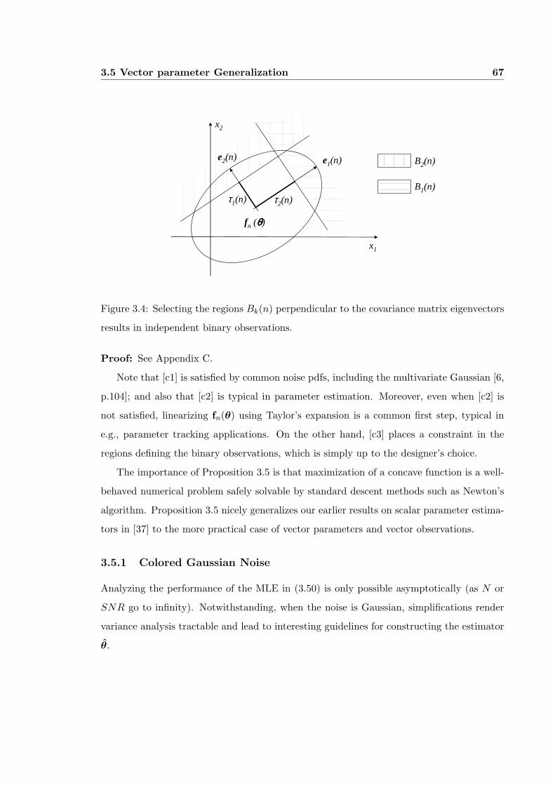
3.5 Vector parameter Generalization 67
x1
x2
B2(n)
B1(n)
fn (θθθθ)
e1(n)
τ2(n)
e2(n)
τ1(n)
Figure 3.4: Selecting the regions Bk(n) perpendicular to the covariance matrix eigenvectors
results in independent binary observations.
Proof: See Appendix C.
Note that [c1] is satisfied by common noise pdfs, including the multivariate Gaussian [6,
p.104]; and also that [c2] is typical in parameter estimation. Moreover, even when [c2] is
not satisfied, linearizing fn(θ) using Taylor’s expansion is a common first step, typical in
e.g., parameter tracking applications. On the other hand, [c3] places a constraint in the
regions defining the binary observations, which is simply up to the designer’s choice.
The importance of Proposition 3.5 is that maximization of a concave function is a well-
behaved numerical problem safely solvable by standard descent methods such as Newton’s
algorithm. Proposition 3.5 nicely generalizes our earlier results on scalar parameter estima-
tors in [37] to the more practical case of vector parameters and vector observations.
3.5.1 Colored Gaussian Noise
Analyzing the performance of the MLE in (3.50) is only possible asymptotically (as N or
SNR go to infinity). Notwithstanding, when the noise is Gaussian, simplifications render
variance analysis tractable and lead to interesting guidelines for constructing the estimator
θ.
3.5 Vector parameter Generalization 68
Restrict pw(w; ψ) ↔ pw(w) to the class of multivariate Gaussian pdfs, and let C(n)
denote the noise covariance matrix at sensor n. Assume that {C(n)}N−1n=0 are known and let
{(em(n), σ2m(n))}M
m=1 be the set of eigenvectors and associated eigenvalues:
C(n) =M∑
m=1
σ2m(n)em(n)eT
m(n). (3.51)
For each sensor, we define a set of K = M regions Bk(n) as half-spaces whose borders are
hyper-planes perpendicular to the covariance matrix eigenvectors; i.e.,
Bk(n) = {x ∈ RM | eTk (n)x ≥ τk(n)}, k = 1, . . . ,K = M, (3.52)
Fig (3.4) depicts the regions Bk(n) in (3.52) for M = 2. Note that since each entry of x(n)
offers a distinct scalar observation, the selection K = M amounts to a bandwidth constraint
of 1 bit per sensor per dimension.
The rationale behind this selection of regions is that the resultant binary observations
bk(n) are independent, meaning that Pr{bk1(n)bk2(n)} = Pr{bk1(n)}Pr{bk2(n)} for k1 6= k2.
As a result, we have a total of MN independent binary observations to estimate θ.
Herein, the Bernoulli parameters qk(n) take on a particularly simple form in terms of
the Gaussian tail function Q(u) := (1/√
2π)∫∞u e−u2/2 du,
qk(n) =
∫
eTk (n)u≥τk(n)
pw(u− fn(θ)) du
= Q
(τk(n)− eT
k (n)fn(θ)σk(n)
):= Q(∆k(n)), (3.53)
where we introduced the σ-distance between fn(θ) and the corresponding threshold
∆k(n) := [τk(n)− eTk (n)fn(θ)]/σk(n).
The independence among binary observations implies that p(b(n)) =∏K
k=1[qk(n)]bk(n)[1−qk(n)]1−bk(n), and leads to a simple log-likelihood function
L(θ) =N−1∑
n=0
K∑
k=1
bk(n) ln qk(n) + [1− bk(n)] ln[1− qk(n)], (3.54)
whose NK independent summands replace the N2K dependent summands in (3.49).

3.5 Vector parameter Generalization 69
Since the regions Bk(n) are half-spaces, Proposition 3.5 applies to the maximization
of (3.54) and guarantees that the numerical search for the θ estimator in (3.54) is well-
conditioned and will converge to the global maximum, at least when the functions fn are
linear. More important, it will turn out that these regions render finite sample performance
analysis of the MLE in (3.50), tractable. In particular, it is possible to derive a closed-form
expression for the Fisher Information Matrix (FIM) [16, p.44], as we establish next.
Proposition 3.6 The FIM, I, for estimating θ based on the binary observations obtained
from the regions defined in (3.52), is given by
I =N−1∑
n=0
JTn
[K∑
k=1
e−∆2k(n)ek(n)eT
k (n)2πσ2
k(n)Q(∆k(n))[1−Q(∆k(n))]
]Jn, (3.55)
where Jn denotes the Jacobian of fn(θ).
Proof: We just have to consider the second derivative of the log-likelihood function in (3.54)
∂2L(θ)∂θ2 =
N−1∑
n=0
K∑
k=1
∂2qk
∂θ2
[bk(n)qk(n)
− 1− bk(n)1− qk(n)
]
− ∂qk
∂θ
∂T qk
∂θ
[bk(n)
[qk(n)]2+
1− bk(n)[1− qk(n)]2
], (3.56)
and take expected value with respect to the binary observations bk(n) to obtain
E[∂2L(θ)
∂θ2
]=
N−1∑
n=0
K∑
k=1
−∂qk
∂θ
∂T qk
∂θ
[1
qk(n)+
11− qk(n)
], (3.57)
where we used the fact that E[bk(n)] = qk(n).
On the other hand, differentiating qk with respect to θ yields [c.f. (3.53)]
∂qk
∂θ=
e−∆2k(n)/2
√2πσk(n)
JTnek(n). (3.58)
The FIM is obtained as the negative of the expected value in (3.57); if we also substi-
tute (3.58) into (3.57), we obtain
I =N−1∑
n=0
K∑
k=1
e−∆2k(n)
2πσ2k(n)
JTnek(n)eT
k (n)Jn1
qk(n)[1− qk(n)]. (3.59)

3.5 Vector parameter Generalization 70
Moving the common factor Jn outside the innermost summation and substituting qk(n) by
its value in (3.53), we obtain (3.55).
The FIM places a lower bound in the achievable variance of unbiased estimators since
the covariance of any estimator must satisfy,
cov(θ)− I−1 º 0 (3.60)
where the notation º 0 stands for positive semidefiniteness of a matrix; the variances in
particular are bounded by var(θk) ≥ [I−1]kk.
Inspection of (3.55) shows that the variance of the MLE in (3.50) depends on the signal
function containing the parameter of interest (via the Jacobians), the noise structure and
power (via the eigenvalues and eigenvectors), and the selection of the regions Bk(n) (via
the σ-distances). Among these three factors only the last one is inherent to the bandwidth
constraint, the other two being common to the estimator that is based on the original x(n)
observations.
The last point is clarified if we consider the FIM Ix for estimating θ given the unquan-
tized vector observations x(n). This matrix can be shown to be (see Appendix D),
Ix =N−1∑
n=0
JTn
[M∑
m=1
em(n)eTm(n)
σ2m(n)
]JT
n . (3.61)
If we define the equivalent noise powers as
ρ2k(n) :=
2πQ(∆k(n))[1−Q(∆k(n))]
e−∆2k(n)
σ2k(n), (3.62)
we can rewrite (3.55) in the form
I =N−1∑
n=0
JTn
[K∑
k=1
ek(n)eTk (n)
ρ2k(n)
]JT
n , (3.63)
which except for the noise powers has form identical to (3.61). Thus, comparison of (3.63)
with (3.61) reveals that from a performance perspective, the use of binary observations is
equivalent to an increase in the noise variance from σ2k(n) to ρ2
k(n), while the rest of the
problem structure remains unchanged.
3.6 Simulations 71
Since we certainly want the equivalent noise increase to be as small as possible, mini-
mizing (3.62) over ∆k(n) calls for this distance to be set to zero, or equivalently, to select
thresholds τk(n) = eTk (n)fn(θ). In this case, the equivalent noise power is
ρ2k(n) =
π
2σ2
k(n). (3.64)
Surprisingly, even in the vector case a judicious selection of the regions Bk(n) results in a
very small penalty (π/2) in terms of the equivalent noise increase. Similar to Sections 3.3.1
and 3.3.2, we can thus claim that while requiring the transmission of 1 bit per sensor per
dimension, the variance of the MLE in (3.50), based on {b(n)}N−1n=0 , yields a variance close
to the clairvoyant estimator’s variance –based on {x(n)}N−1n=0 – for low-to-medium Q-SNR
problems.
3.6 Simulations
3.6.1 Scalar parameter estimation
We begin by simulating the estimator in (3.14) for scalar parameter estimation in the
presence of AWGN with unknown variance. Results are shown in Fig. 3.5 for two different
sets of σ-distances, ∆1, ∆2, corroborating the values predicted by (3.15) and the fact that
the performance loss with respect to the clairvoyant sample mean estimator, x, is indeed
small.
Without invoking assumptions on the noise pdf, we also tested the simplified estimator
in (3.40). Fig. 3.6 shows one such test, depicting the bound in (3.39) as well as simulated
variances for uniform and Gaussian noise pdfs. Note that the bound overestimates the
variance by a factor of roughly 2 for the uniform case and roughly 4 for the Gaussian case.
Note that having unbounded derivative, the uniform pdf is not covered by Proposition 3.3;
however, for piecewise linear CCDFs of which uniform noise is a special case, (3.34) does
not hold true but the error of the trapezoidal rule ea is small anyways, as testified by the
corresponding points in Fig. 3.6
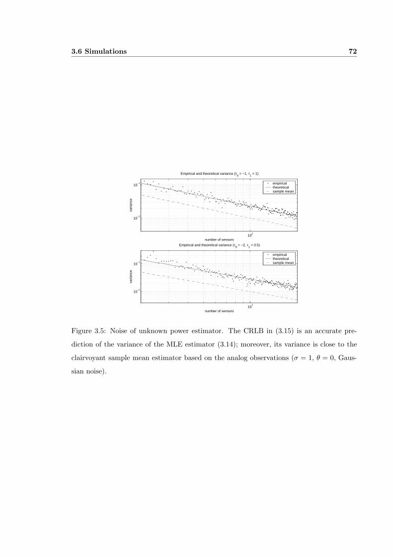
3.6 Simulations 72
102
10−2
10−1
Empirical and theoretical variance (τ0 = −1, τ
1 = 1)
number of sensors
varia
nce
empiricaltheoreticalsample mean
102
10−2
10−1
Empirical and theoretical variance (τ0 = −2, τ
1 = 0.5)
number of sensors
varia
nce
empiricaltheoreticalsample mean
Figure 3.5: Noise of unknown power estimator. The CRLB in (3.15) is an accurate pre-
diction of the variance of the MLE estimator (3.14); moreover, its variance is close to the
clairvoyant sample mean estimator based on the analog observations (σ = 1, θ = 0, Gaus-
sian noise).

3.6 Simulations 73
102
10−1
100
Empirical and theoretical variance for first component of v
number of sensors
varia
nce
empirical (gaussian noise)empirical (uniform noise)variance bound
Figure 3.6: Universal estimator introduced in Section 3.4. The bound in (3.39) overestimates
the real variance by a factor that depends on the noise pdf (σ = 1, T = 5, θ chosen randomly
in [−2, 2])
x0
x1
φ (n)
n
v
Figure 3.7: The vector flow v incises over a certain sensor capable of measuring the normal
component of v.

3.6 Simulations 74
102
10−2
10−1
Empirical and theoretical variance for first component of v
number of sensors
varia
nce
empiricaltheoreticalanalog MLE
102
10−2
10−1
Empirical and theoretical variance for second component of v
number of sensors
varia
nce
empiricaltheoreticalanalog MLE
Figure 3.8: Average variance for the components of v. The empirical as well as the
bound (3.68) are compared with the analog observations based MLE (v = (1, 1), σ = 1).
3.6.2 Vector Parameter Estimation – A Motivating Application
In this section, we illustrate how a problem involving vector parameters can be solved using
the estimators of Section 3.5.1. Suppose we wish to estimate a vector flow using incidence
observations. With reference to Fig. 3.7, consider the flow vector v := (v0, v1)T , and a
sensor positioned at an angle φ(n) with respect to a known reference direction. We will rely
on a set of so called incidence observations {x(n)}N−1n=0 measuring the component of the flow
normal to the corresponding sensor
x(n) := 〈v,n〉+ w(n) = v0 sin[φ(n)] + v1 cos[φ(n)] + w(n), (3.65)
where 〈, 〉 denotes inner product, w(n) is zero-mean AWGN, and the equation holds for
n = 0, 1, . . . , N − 1. The model (3.65) applies to the measurement of hydraulic fields,
pressure variations induced by wind and radiation from a distant source [25].
Estimating v fits the framework of Section 3.5.1 requiring the transmission of a single
binary observation per sensor, b1(n) = 1{x(n) ≥ τ1(n)}. The FIM in (3.63) is easily found

3.6 Simulations 75
to be
I =N−1∑
n=0
1ρ21(n)
sin2[φ(n)] sin[φ(n)] cos[φ(n)]
sin[φ(n)] cos[φ(n)] cos2[φ(n)]
. (3.66)
Furthermore, since x(n) in (3.65) is linear in v and the noise pdf is log-concave (Gaussian)
the log-likelihood function is concave as asserted by Proposition 3.5.
Suppose that we are able to place the thresholds optimally at τ1(n) = v0 sin[φ(n)] +
v1 cos[φ(n)], so that ρ21(n) = (π/2)σ2. If we also make the reasonable assumption that the
angles are random and uniformly distributed, φ(n) ∼ U [−π, π], then the average FIM turns
out to be:
I =2
πσ2
N/2 0
0 N/2
. (3.67)
But according to the law of large numbers I ≈ I, and the estimation variance will be
approximately given by
var(v0) = var(v1) =πσ2
N. (3.68)
Fig. 3.8 depicts the bound (3.68), as well as the simulated variances var(v0) and var(v1)
in comparison with the clairvoyant MLE based on {x(n)}N−1n=0 , corroborating our analytical
expressions. While this excellent performance is obtained under ideal threshold placement,
recalling the harsh bandwidth constraint (1 bit per sensor) justifies the potential of our
approach for bandwidth-constrained distributed parameter estimation in this WSN-based
context.

3.7 Appendices 76
3.7 Appendices
3.7.1 Proofs of Lemma 3.1 and Proposition 3.2
Lemma 3.1
That q is unbiased follows from the linearity of expectation and the fact that q = E[b(n)].
We will also establish that q is the MLE using Cramer-Rao’s theorem; the result will
actually be stronger since q is in fact the Minimum Variance Unbiased Estimator (MVUE)
of q. To this end, using that τ2 > τ1, the log-likelihood function takes on the form
L(b,q) =N−1∑
n=0
[1− b1(n)][1− b2(n)] ln Pr{x(n) < τ1}
+ b1(n)[1− b2(n)] ln Pr{τ1 < x(n) < τ2}
+ b1(n)b2(n) ln Pr{τ2 < x(n)}. (3.69)
Note that we can rewrite the probabilities in terms of the components of q, since e.g.,
Pr{τ1 < x(n) < τ2} = q1 − q2. Moreover, since the binary observations are either 0 or 1
and the combination b(n) = (0, 1) is impossible, we can simplify the products of binary
observations; e.g., b1(n)[1− b2(n)] = b2(n)− b1(n). Enacting these simplifications in (3.69),
we obtain
L(b,q) =N−1∑
n=0
[1− b1(n)] ln[1− q1]
+[b1(n)− b2(n)] ln[q1 − q2] + b2(n) ln q2. (3.70)
From (3.70), we can obtain the gradient of L(b,q) as
∂L
∂q=
N−1∑
n=0
1−b1(n)1−q1
+ b1(n)−b2(n)q1−q1
− b1(n)−b2(n)q1−q1
+ b2(n)q2
= N
1−q1(n)1−q1
+ q1(n)−q2(n)q1−q1
− q1(n)−q2(n)q1−q1
+ q2(n)q2
. (3.71)
Differentiating once more yields the Hessian, and taking expected value over b yields the
FIM:
I(q) =N
q1 − q2
1−q2
1−q1−1
−1 q1
q2
. (3.72)

3.7 Appendices 77
It is a matter of simple algebra to verify that ∂L/∂q = I(q)[q− q], from where application
of Cramer-Rao’s theorem concludes the proof of Lemma 3.1.
Proposition 3.2
The proof is analogous to the one of Proposition 3.1. Let us start by inverting I(q)
[c.f. (3.72)],
I−1(q) =1N
(1− q1)q1 (1− q1)q2
(1− q1)q2 (1− q2)q2
. (3.73)
We can now apply the property stated in (3.19), with the inverse FIM given by (3.73), to
obtain
var(θ) ≥(
∂θ
∂q1
)2 q1(1− q1)N
+(
∂θ
∂q2
)2 q2(1− q2)N
+(
∂θ
∂q1
)(∂θ
∂q2
)q2(1− q1)
N. (3.74)
Substituting the derivatives from (3.20) into (3.74) completes the proof of Proposition 3.2.
3.7.2 Proofs of Lemma 3.2 and Proposition 3.4
Lemma 3.2
As in the proof of Lemma 3.1, the key property is that only some combinations of binary
observations are possible; hence, we have
b1(n) . . . bk(n)[1− bk+1(n)] . . . [1− bK(n)] = bk − bk+1, (3.75)
and the log-likelihood function takes the form
L(q,b) =N−1∑
n=0
K∑
k=0
[bk(n)− bk+1(n)] ln(qk − qk−1)
= N
K∑
k=0
[qk(n)− qk+1(n)] ln(qk − qk−1), (3.76)
where for the last equality we interchanged summations and substituted qk from (3.42).

3.7 Appendices 78
Applying the Neyman-Fisher factorization theorem to (3.76), we deduce that {qk}Kk=1
are sufficient statistics for estimating q [16, p.104]. Furthermore, noting that E(q) = q and
that q is a function of sufficient statistics, application of Rao-Blackwell-Lehmann-Scheffe
theorem proves that q is the MVUE (and consequently the MLE) of q.
To compute the covariance, recall that E(bk(n)) = qk to find that
cov[bk(n), bl(n)] := E[(bk(n)− qk)(bl(n)− ql)]
= E[bk(n)bl(n)]− qkql
= ql − qkql; (3.77)
where for the last equality we used that E[bk(n)bl(n)] = Pr{bk(n) = 1, bl(n) = 1} = ql, for
l ≥ k. The proof follows form the independence of binary observations across sensors:
cov[qk(n), ql(n)] =1
N2
N−1∑
n=0
cov[bk(n), bl(n)] =ql(1− qk)
N. (3.78)
QED.
Proposition 3.4
To compute the variance of θ, use the linearity of expectation to write
var(θ) =K∑
k=1
K∑
l=1
(τk+1 − τk−1)(τl+1 − τl−1)4
E[(qk(n)− qk)(ql(n)− ql)]. (3.79)
Note that the expected value is by definition E[(qk(n)− qk)(ql(n)− ql)] = cov[bk(n), bl(n)],
and is thus given by (3.43) when l ≥ k. Substituting these values into (3.79), we obtain
var(θ) =K∑
k=1
(τk+1 − τk−1)2
4qk(1− qk)
N
+ 2K∑
k=1
∑
l>k
(τk+1 − τk−1)(τl+1 − τl−1)4
ql(1− qk)N
. (3.80)
Finally, note that ql(1− qk) ≤ 1/4 and that τk+1 − τk−1 < 2τmax, to arrive at:
var(θ) ≤K∑
k=1
τ2max
4N+
K∑
k=1
∑
l>k
τ2max
2N. (3.81)
Since the first sum contains K terms and the second K(K − 1)/2, (3.44) follows.

3.7 Appendices 79
3.7.3 Proof of Proposition 3.5
Consider the indicator function associated with Bβ(n)
g(w) =
1 w ∈ Bβ(n)
0 else. (3.82)
Eq. (3.47) and [c3], imply that since Bβ(n) is an intersection of half-spaces, it is convex (in
fact [c3] is both sufficient and necessary for the convexity of Bβ(n), ∀ β). Since g(w) is the
indicator function of a convex set it is log-concave (and concave too).
Now, let us rewrite (3.48) as
qβ(n) =∫
RM
g(w + Hnθ)pw(w) dw, (3.83)
and use the fact that g(w+Hnθ) is log-concave in its argument. Moreover, since [c2] makes
this argument affine in (w, θ), it follows that g(w + Hnθ) is log-concave in (w, θ). Since
pw(w) is log-concave under [c1], the product g(w + Hnθ)pw(w) is log-concave too.
At this point, we can apply the integration property of log-concave functions to claim
that qβ(n) is log-concave, [6, p.104]. Finally, note that L(θ) comprises the sum of logarithms
of log-concave functions; thus, each term is concave and so is their sum.
D. FIM for estimation of θ based on {x(n)}N−1n=0
Let x := (xT (0),xT (1), . . . ,xT (N − 1))T and consider the log-likelihood
ln px(x, θ) =N−1∑
n=0
12
ln[(2π)M det(C(n))]
− 12[x(n)− fn(θ)]TC−1(n)[x(n)− fn(θ)]. (3.84)
Differentiating twice with respect to θ, we obtain the first
∂ ln px(x, θ)∂θ
=N−1∑
n=0
JTnC−1(n)[x(n)− fn(θ)], (3.85)
and second derivative
∂2 ln px(x, θ)∂θ2 =
N−1∑
n=0
∂JTn
∂θC−1(n)[x(n)− fn(θ)] + JT
nC−1(n)Jn. (3.86)

3.7 Appendices 80
Since E[x(n)] = fn(θ), taking the negative of the expected value in (3.86) yields the FIM
Ix =N−1∑
n=0
JTnC−1(n)Jn. (3.87)
Now, recall that the eigenvalues of C−1(n) are the inverses of the eigenvalues of C(n),
and the eigenvectors are equal. Finally, use C−1(n) =∑M
m=1 σ−2m (n)em(n)eT
m(n) to ob-
tain (3.61).
81
Chapter 4
Distributed state estimation using
the sign of innovations
4.1 Introduction
In Chapters 2 and 3 we considered tradeoffs when estimating signals using very noisy sensor
data. We concluded that as the noise variance becomes comparable with the parameter’s
dynamic range, quantization to a single bit per observation leads to low complexity estima-
tors of time-invariant deterministic parameters with minimal information loss. This holds
true for a large class of problems, where the noise probability distribution function (pdf)
may be parametrically described or even unknown.
Taking into account the stringent bandwidth constraints of WSNs, this chapter studies
state estimation of dynamical stochastic processes based on severely quantized observations,
whereby low-cost communications restrict sensors to transmit a single bit per observation.
The quantization rule manifests itself in a non-linear measurement equation in a Kalman
Filtering (KF) setup. While the discontinuous non-linearity precludes application of the
extended (E)KF, it can be handled with more powerful techniques such as the unscented
(U)KF [15], or the Particle Filter (PF) [10,18] – algorithms that have also been applied in
the context of filtering [8, 45] and target tracking with a WSN [2, 11]. However, all these
approaches are significantly more complex than a KF and, besides, no insight has been pro-
4.1 Introduction 82
vided with regards to their performance degradation when quantized data are used in lieu of
the analog-amplitude observations. The contribution of the present chapter is precisely to
address these two issues with the goal being to construct state estimators based on binary
observations so that:
i) complexity is rendered comparable to the equivalent KF based on the original observa-
tions; and,
ii) the mean squared error (MSE) of the resultant estimate based on binary observations is
close to the MSE of the estimate based on the original observations.
We begin by introducing our WSN setup and formulating the problem in Section 4.2,
where we delineate the KF that we will use to benchmark algorithms in the rest of the
chapter (Section 4.2.1). State estimation based on the sign of innovations (SOI) is considered
first for a vector state - scalar observation model in Section 4.3, where we discuss the
minimum mean squared error (MMSE) estimator (Section 4.3.1). As the latter may be
prohibitive for a resource-limited WSN, we pursue a reduced-complexity approximation in
Section 4.3.2 which leads to the SOI-KF algorithm whose complexity and performance are
surprisingly close to the clairvoyant KF, even when inter-sensor communication relies on
the low-cost transmission of a single bit per sensor. These results are extended to a general
vector state - vector parameter model in Section 4.4. The performance of the SOI-KF is
analyzed in Section 4.5, where using the underlying continuous-time physical processes we
show that the MSE of the SOI-KF is closely related to the MSE of a KF with only π/2
larger noise covariance matrix. We present a motivating example in Section 4.6, entailing
temperature monitoring with a WSN. Finally, we apply a modified version of the SOI-KF
to the canonical problem of distributed target tracking based on binary observations in
Section 4.6.1.
Notation: We use p(x|y; z) to denote the probability density function (pdf) of the random
variable (r.v.) x given the r.v. y evaluated at z; when using the same letter to denote the
r.v. and the argument of the pdf we abbreviate p(x|y;x) = p(x|y). When a r.v. is normally
distributed with mean µx = E(x) and covariance matrix Cx = E(xxT ), we write p(x) =

4.2 Problem statement and preliminaries 83
x(n) = Ax(n-1) + u(n)
+ + +x(0) v(0)
. . . .
S(0) S(1) S(n)
b(0) b(1) b(n)
x(1) v(1) x(n) v(n)
Figure 4.1: Ad hoc WSN: the network itself is in charge of tracking the state x(n)
N (x;µx,Cx), where T stands for transposition. In the particular case of a scalar r.v., we
write p(x) = N (x; µx, σ2x) and define the Gaussian tail function as Q(x) :=
∫∞x N (u; 0, 1)du.
We will use δc(t) to denote the Dirac delta function defined by δc(t) = 0 ∀t 6= 0, and∫∞−∞ δc(t)dt = 1; and δ(n) to denote the Kronecker delta function defined as δ(0) = 1 and
δ(n) = 0 ∀n 6= 0. Throughout the chapter, I will denote the identity matrix, and lower
(upper) case boldface letters will stand for column vectors (matrices).
4.2 Problem statement and preliminaries
We are primarily concerned with so called ad-hoc WSNs in which the network itself is
responsible for collecting and processing information; see Fig. 4.1. Let us consider an ad-
hoc WSN with K distributed sensors {Sk}Kk=1 deployed with the objective of tracking a p×1
real random vector (state) xc(t) ∈ Rp. The state evolution in continuous-time is described
by
xc(t) = Ac(t)xc(t) + uc(t), (4.1)
where Ac(t) ∈ Rp×p, and the driving input uc(t) ∈ Rp is a zero-mean white Gaussian
process with autocorrelation E[uc(t1)uTc (t2)] = Cuc(t1)δc(t1 − t2). The sensors observe the
state xc(t) through a linear transformation. Letting yc(t, k) ∈ RM denote the observation
at sensor Sk, we have
yc(t, k) = Hc(t, k)xc(t) + vc(t, k), (4.2)

4.2 Problem statement and preliminaries 84
where Hc(t, k) ∈ RM×p and the observation noise vc(t, k) ∈ RM is also a zero-mean Gaus-
sian process with E[vc(t1, k1)vTc (t2, k2)] = Cvc(t1, k1)δc(t1 − t2)δ(k1 − k2); i.e., the noise is
uncorrelated across time and sensors.
To track xc(t), we consider uniform sampling with period Ts and define the discrete-time
state and observations as x(n) := xc(nTs) and y(n, k) := yc(nTs, k), respectively. Using the
continuous-time model described by (4.1) and (4.2) we can obtain an equivalent discrete-
time model [26, Section 4.9]. Upon defining Φ(t2, t1) := exp[∫ t2
t1Ac(t)dt
], we can solve the
differential equation in (4.1) between (n − 1)Ts and nTs with initial condition x(n − 1) to
obtain
x(n) = Φ(nTs, (n− 1)Ts)x(n− 1) +∫ nTs
(n−1)Ts
Φ(nTs, τ)uc(τ)dτ. (4.3)
For simplicity, define the matrix A(n) := Φ(nTs, (n − 1)Ts) and the white Gaussian driv-
ing noise input u(n) :=∫ nTs
(n−1)TsΦ(nTs, τ)uc(τ)dτ . With these definitions, the resultant
discrete-time equivalent model is given by the vector time-varying autoregressive (AR) pro-
cess
x(n) = A(n)x(n− 1) + u(n)
y(n, k) = H(n, k)x(n) + v(n, k). (4.4)
where H(n, k) := Hc(nTs, k) and the observation noise is white Gaussian with pdf
p[v(n, k)] = N [v(n, k);0,Cv(n, k)]. Since sampling (4.2) requires passing yc(t, k) through
a low- or band-pass filter of bandwidth 1/Ts, the sampled covariance matrix satisfies
Cv(n, k) := E[v(n, k)vT (n, k)] = Cvc(nTs, k)/Ts [26, Section 4.9]. Finally, note that
u(n)’s definition implies that p[u(n)] = N [u(n); 0,Cu(n)] with covariance matrix Cu(n) :=
E[u(n)uT (n)] =∫ nTs
(n−1)TsΦ(nTs, τ)Cuc(τ)ΦT (nTs, τ)dτ .
Supposing that A(n), Cu(n), H(n, k) and Cv(n, k) are available ∀ n, k, the goal of
the WSN is for each sensor Sk to form an estimate of x(n) to be used in e.g., a habitat
monitoring application [25], or, as a first step in e.g., a distributed control setup. In any
event, estimating x(n) necessitates each sensor Sl to communicate y(n, l) to the remaining
sensors {Sk}Kk=1,k 6=l. This communication takes place over the shared wireless channel that
we will assume can afford transmission of a single packet per time slot n, leading to a

4.2 Problem statement and preliminaries 85
one-to-one correspondence between time n and sensor index k and allowing us to drop the
sensor argument k in (4.4). The decision of which sensor Sk = S(n) is active at time n, and
consequently which observation y(n, k) = y(n) gets transmitted, depends on the underlying
scheduling algorithm – see e.g.; [7] and references therein – but is assumed given for the
purpose of this paper. Digital transmission of y(n) also implies some form of quantization
qn to map the analog observations y(n) into binary data:
b(n) := qn(y(n)), with qn : RM → {0, 1}M , (4.5)
where b(n) := [b(n, 1), . . . , b(n,M)]T is an M -component binary message. Implicit to (4.5)
is the fact that we are restricting the sensors to transmit one bit per scalar observation
which effects low-cost communications among sensors. Indeed, the quantization function
qn partitions RM in 2M regions, implying that on the average each component of y(n) is
quantized to 1 bit. We further suppose that the messages b(n) are correctly received by all
sensors, which assumes deployment of sufficiently powerful error control codes.
The objective of this paper is to derive and analyze the performance of MMSE estima-
tors of x(n) based on the messages b0:n := [bT (0), . . . ,bT (n)]T that are available to each
and every sensor. It is well known that the MMSE estimator is given by the conditional
expectation [16, Chap. 12]; consequently, if we let x(n|n) denote the MMSE estimator of
x(n) given b0:n, we have
x(n|n) := E[x(n)|b0:n] =∫
Rp
x(n)p[x(n)|b0:n]dx(n). (4.6)
Instrumental to the ensuing derivations are the so called predictors that estimate (predict)
the state and observation vectors based on past observations:
x(n|n− 1) := E[x(n)|b0:n−1] = A(n)x(n− 1|n− 1)
y(n|n− 1) := E[y(n)|b0:n−1] = H(n)x(n|n− 1). (4.7)
For each of the state estimators in (4.6) and (4.7), we define the error covariance matrices
(ECM) M(n|n) := E[(x(n|n) − x(n))(x(n|n) − x(n))T ], and M(n|n − 1) := E[(x(n|n −1) − x(n))(x(n|n − 1) − x(n))T ] for the filtered and the predicted estimate, respectively.

4.2 Problem statement and preliminaries 86
x(n) = Ax(n-1) + u(n)
+ + +x(0) v(0)
. . . .
S(0) S(1) S(n)
b(0) b(1) b(n)
x(1) v(1) x(n) v(n)
F u s i o n C e n t e r
f(n) = b(n)
Figure 4.2: WSN with a Fusion Center: the sensors act as data gathering devices.
The mean-squared errors (MSE) of x(n|n) and x(n|n − 1) are given by tr[M(n|n)] and
tr[M(n|n− 1)] with these traces being minimum among all possible estimators x(n|n) and
x(n|n− 1) of x(n). The ECM of the state predictor can be obtained from the ECM of the
state estimator through the recursion
M(n|n− 1) = A(n)M(n− 1|n− 1)AT (n) + Cu(n), (4.8)
which we will use in later derivations. Note that the relations between x(n|n − 1) and
x(n−1|n−1) and y(n|n−1) and x(n|n−1) in (4.7) and between M(n|n−1) and M(n−1|n−1)
in (4.8) follow from the linearity of the expected value operator and are independent of the
quantization rule in (4.5).
Remark 4.1 When a fusion center (FC) is present, the WSN is termed hierarchical in
the sense that sensors act as information gathering devices for the FC that is in charge of
processing this information; see Fig. 4.2. Results in this paper also apply to networks of
this type provided that the FC feeds back to the sensors packets f(n) := b(n). As we will
discuss in Sections 4.3.2 and 4.4, the sole condition for applying the proposed method is to
have the predicted observation y(n|n− 1) available at S(n), a condition that can be met in
the hierarchical WSN with feedback f(n) = b(n).

4.2 Problem statement and preliminaries 87
4.2.1 The Kalman filter benchmark
Before considering estimation based on binary observations, let us highlight some proper-
ties of the clairvoyant KF that will come handy in subsequent derivations. Consider for
simplicity a vector state - scalar observation model described by
x(n) = A(n)x(n− 1) + u(n)
y(n) = hT (n)x(n) + v(n). (4.9)
The model in (4.9) is a particular case of the general model (4.4) in which M = 1; the
observations y(n) ↔ y(n), noise v(n) ↔ v(n) and noise covariance Cv(n) ↔ σ2v(n) are
scalar; and H(n) ↔ hT (n) ∈ R1×p is a row vector.
If we had infinite bandwidth available, we could communicate the observations y(n)
error-free. This is rightfully a clairvoyant benchmark for our bandwidth-constrained esti-
mators and corresponds to the problem setup of Section 4.2 with messages b(n) = y(n).
In this case, we have a well known linear Gaussian vector AR estimation problem whose
MMSE can be recursively obtained by the KF [16, Chap. 13]. Assuming that the estimate
x(n − 1|n − 1) and the ECM M(n − 1|n − 1) are known at step n − 1, we compute the
predicted estimate x(n|n−1) and the corresponding ECM M(n|n−1) using (4.7) and (4.8),
respectively. Next, the filtered estimate x(n|n) is obtained by solving the integral in (4.6)
with the posterior pdf computed by means of Bayes’ rule
p[x(n)|y0:n] =p[y(n)|x(n),y0:n−1]p[x(n)|y0:n−1]
p[y(n)|y0:n−1]. (4.10)
The key observation is that because of the linear Gaussian model (4.9), the posterior
p[x(n)|y0:n] = N [x(n); x(n|n),M(n|n)] is normal, leading to the so called correction step
x(n|n) = x(n|n− 1) +M(n|n− 1)h(n)
hT (n)M(n|n− 1)h(n) + σ2v(n)
[y(n)− y(n|n− 1)]
M(n|n) = M(n|n− 1)− M(n|n− 1)h(n)hT (n)M(n|n− 1)hT (n)M(n|n− 1)h(n) + σ2
v(n), (4.11)
which yields the filtered estimate x(n|n) and its MSE M(n|n). Recursive application
of (4.7), (4.8) and (4.11) yields the MMSE estimate of x(n) given y0:n.

4.3 State estimation using the sign of innovations 88
4.3 State estimation using the sign of innovations
The corrector in (4.11) depends on the innovation sequence y(n|n− 1) := y(n)− y(n|n− 1)
corresponding to the difference between the current observation and the prediction based
on past observations. This suggests that a convenient form for the quantization function
qn is qn[y(n) − y(n|n − 1)]. We start by considering the vector state - scalar observation
model in (4.9) and define the message b(n) as the sign of innovation (SOI):
b(n) = sign[y(n)− y(n|n− 1)] :=
+1, if y(n) ≥ y(n|n− 1)
−1, if y(n) < y(n|n− 1). (4.12)
Notice that the SOI b(n) is not a standard quantizer of the data y(n). It can be thought as
one with judiciously setting the quantization threshold at the data prediction y(n|n − 1).
The focus of the present section is to study MMSE estimation of x(n) based on b0:n :=
[b(0), . . . , b(n)]T .
4.3.1 Exact MMSE Estimator
To find the MMSE in (4.6) based on the SOI in (4.12) we can, in principle, proceed as we
described in Section 4.2.1 for the KF. However, while we can update the estimate x(n−1|n−1) and its ECM M(n−1|n−1) using (4.7) and (4.8) to obtain the predictor x(n|n−1) and
its corresponding ECM M(n|n−1), the analogy with the KF cannot be pursued any further.
The reason is that due to the non-linearity in the definition of b(n) in (4.12) the distribution
p[x(n)|b0:n−1] is no longer normal; and thus, its description requires additional information
besides its mean and variance. This characteristic problem of non-linear filtering motivates
the need for a means of propagating the posterior pdf p[x(n)|b0:n] so that the integral
in (4.6) can be evaluated. Such a rule is described in the following proposition.
Proposition 4.1 Consider the vector state - scalar observation model defined by (4.9),
and the SOI messages defined as in (4.12). Then, the posterior pdf of x(n) given the binary

4.3 State estimation using the sign of innovations 89
observations b0:n can be obtained using the recursions:
p[x(n)|b0:n−1] =∫
Rp
p[x(n− 1)|b0:n−1]N [x(n);A(n)x(n− 1),Cu(n)]dx(n− 1)(4.13)
p[x(n)|b0:n] = αnQ
[−b(n)
hT (n)[x(n)− x(n|n− 1)]σv(n)
]p[x(n)|b0:n−1] (4.14)
where αn is a normalizing constant ensuring that∫Rp p[x(n)|b0:n]dx(n) = 1.
Proof: The prior pdf p[x(n)|b0:n−1] in (4.13) follows from the theorem of total probability:
p(x(n)|b0:n−1) =∫
Rp
p[x(n)|x(n− 1),b0:n−1]p[x(n− 1)|b0:n−1]dx(n− 1). (4.15)
Note however that since x(n−1) is given in p[x(n)|x(n−1),b0:n−1], conditioning on b0:n−1
is irrelevant and p[x(n)|x(n−1),b0:n−1] = p[x(n)|x(n−1)] = N [x(n);A(n)x(n−1),Cu(n)]
yielding (4.13). The posterior pdf in (4.14) can be obtained from Bayes’ rule
p[x(n)|b0:n−1, b(n)] =p[b(n)|x(n),b0:n−1]p[x(n)|b0:n−1]
p[b(n)|b0:n−1]. (4.16)
But the term p[b(n)|x(n),b0:n−1] := Pr{b(n) = ±1|x(n),b0:n−1} can be easily expressed in
terms of the Gaussian tail function
Pr{b(n) = ±1|x(n),b0:n−1} = Pr{y(n) ≷ y(n|n− 1)|x(n)}
= Pr{v(n) ≷ hT (n)[x(n|n− 1)− x(n)]|x(n)}
= Q
[±hT (n)[x(n|n− 1)− x(n)]
σv(n)
], (4.17)
where the first equality follows from the definition of the SOI b(n) in (4.12) and the fact
that since x(n) is given we can ignore the conditioning on b0:n−1; the second equality is
obtained by substituting y(n) for the observation model expression in (4.9); and the last
equality is a consequence of the observations’ noise distribution, p[v(n)] = N [v(n); 0, σ2v(n)].
Substituting (4.17) into (4.16) yields (4.14) after setting αn := 1/Pr{b(n) = ±1|b0:n−1}.
Two recursive algorithms for computing the MMSE x(n|n) can be derived from Propo-
sition 4.1. Algorithm 1-A is ran at the sensors when the scheduling algorithm dictates that
is their turn to transmit the SOI. At this time slot, the sensor computes the distribution

4.3 State estimation using the sign of innovations 90
Algorithm 1–A Exact MMSE estimation – Observation and transmissionRequire: p[x(n)|b0:n−1]
Ensure: b(n)
1: Obtain the distribution p[x(n)|b0:n−1] using (4.13)
2: Compute the prediction x(n|n− 1) =∫Rp x(n)p[x(n)|b0:n−1]dx(n)
3: Find y(n|n− 1) = hT (n)x(n|n− 1)
4: Construct b(n) as in (4.12)
5: Transmit b(n)
Algorithm 1–B Exact MMSE estimation – Reception and estimationRequire: prior distribution p[x(−1)]
1: for n = 0 to ∞ do {repeat for the life of the network}2: Obtain the distribution p[x(n)|b0:n−1] using (4.13)
3: Receive b(n)
4: Obtain the posterior distribution p[x(n)|b0:n] using (4.14)
5: Form the desired estimate, x(n|n) =∫Rp x(n)p[x(n)|b0:n]dx(n).
6: end for
p[x(n)|b0:n−1] using (4.13) from where it predicts the state value by numerically evaluating
x(n|n − 1) =∫Rp x(n)p[x(n)|b0:n−1]dx(n). Based on this prediction, the sensor evaluates
y(n|n − 1) = hT (n)x(n|n − 1) as in (4.7) in order to obtain and transmit the SOI b(n)
as defined in (4.12). Algorithm 1-B is ran by all sensors during the life of the network to
keep track of the state x(n) via the filtered estimate (corrector) x(n|n). To this end, all
sensors compute the pdf p[x(n)|b0:n−1] using (4.13), and subsequently apply (4.14) to find
p[x(n)|b0:n]. The estimate of interest x(n|n) is obtained by numerical integration of the
expression in (4.6).
Albeit optimal, the process described by Algorithms 1-A and 1-B requires numerical
integration at three different times. We first have to evaluate the integral necessary to obtain
p[x(n)|b0:n−1] as stated in (4.13) for step 1 of Algorithm 1-A and step 2 of Algorithm 1-B.
A second numerical integration in step 2 of Algorithm 1-A is required to compute x(n|n−1)
and another one in step 5 of Algorithm 1-B to compute the desired estimate, x(n|n). As

4.3 State estimation using the sign of innovations 91
these can be prohibitively expensive for a resource limited WSN, we are motivated to pursue
a reduced-complexity approximation that we introduce next.
4.3.2 Approximate MMSE estimator
A customary simplification in non-linear filtering is to assume that the pdf p[x(n)|b0:n−1] =
N [x(n); x(n|n− 1),M(n|n− 1)] is Gaussian; see e.g., [18]. In general, the normal approx-
imation of p[x(n)|b0:n−1] is introduced to reduce the problem of tracking the evolution of
a pdf to that of tracking its mean x(n|n − 1) and covariance M(n|n − 1). For the prob-
lem at hand though, it also leads to a very simple algorithm as asserted by the following
proposition.
Proposition 4.2 Consider the vector state - scalar observation model in (4.9) and binary
observations defined as in (4.12). If p[x(n)|b0:n−1] = N [x(n); x(n|n− 1),M(n|n− 1)], then
the MMSE estimator x(n|n) can be obtained from the recursions:
x(n|n− 1) = A(n)x(n− 1|n− 1) (4.18)
M(n|n− 1) = A(n)M(n− 1|n− 1)AT (n) + Cu(n) (4.19)
x(n|n) = x(n|n− 1) +(√
2/π)M(n|n− 1)h(n)√hT (n)M(n|n− 1)h(n) + σ2
v(n)b(n) (4.20)
M(n|n) = M(n|n− 1)− (2/π)M(n|n− 1)h(n)hT (n)M(n|n− 1)hT (n)M(n|n− 1)h(n) + σ2
v(n). (4.21)
Proof: The predictor recursions (4.18) and (4.19) are identical to (4.7) and (4.8), re-
spectively, and are included here for completeness. To establish (4.20), recall that the
conditional mean can be obtained by averaging x(n) over the posterior pdf p[x(n)|b0:n]:
x(n|n) := E[x(n)|b0:n] =∫
Rp
x(n)p[x(n)|b0:n]dx(n). (4.22)
Using Bayes’ rule, we can find the posterior p[x(n)|b0:n] = p[x(n)|b0:n−1, b(n)] as
p[x(n)|b0:n−1, b(n)] =p[b(n)|x(n),b0:n−1]p[x(n)|b0:n−1]
p[b(n)|b0:n−1]. (4.23)
We now examine the three terms in the right hand side of (4.23). The first one is
p[b(n)|x(n),b0:n−1] := Pr{b(n) = ±1|x(n),b0:n−1}, which after repeating the steps used

4.3 State estimation using the sign of innovations 92
to establish (4.17) in the proof of Proposition 4.1 can be expressed in terms of the Gaussian
tail function
Pr{b(n) = ±1|x(n),b0:n−1} = Q
[±hT (n)[x(n|n− 1)− x(n)]
σv(n)
]. (4.24)
To obtain an expression for the term p[b(n)|b0:n−1] := Pr{b(n) = ±1|b0:n−1}, we use the
normal assumption on the distribution of p[x(n)|b0:n−1] to obtain
Pr{b(n) = ±1|b0:n−1} = Pr{y(n) ≷ y(n|n− 1)|b0:n−1} = 1/2, (4.25)
where the first equality follows from the definition of b(n) in (4.12). To obtain the second
equality note that Gaussianity of p[x(n)|b0:n−1] implies that of p[y(n)|b0:n−1] since y(n) is
a linear transformation of x(n); and also that the probability of a normal variable to be
greater or smaller than its mean equals 1/2.
Substituting (4.24) and (4.25) into (4.23) and using the (assumed) normal distribution
p[x(n)|b0:n−1] = N [x(n); x(n|n− 1),M(n|n− 1)], we obtain an expression for the posterior
distribution p[x(n)|b0:n] that we substitute in (4.22) to arrive at
x(n|n) = 2∫
Rp
x(n)N [x(n); x(n|n− 1),M(n|n− 1)]Q[±hT (n)[x(n|n− 1)− x(n)]
σv(n)
]dx(n).
(4.26)
In the Appendix, we prove that the integral in (4.26) can be reduced to (4.20).
To obtain (4.21), we write x(n|n) = x(n|n − 1) + k(n)b(n) with the explicit value of
k(n) as deduced from (4.20), so that we can write the ECM as
M(n|n) := E[(x(n)− x(n|n− 1)− k(n)b(n)) (x(n)− x(n|n− 1)− k(n)b(n))T
]
= M(n|n− 1) + k(n)kT (n)E[b2(n)]− 2k(n)E[b(n)xT (n)], (4.27)
where the first equality follows by definition and in the second equality we used that M(n|n−1) := E[(x(n) − x(n|n − 1))(x(n) − x(n|n − 1))T ]. The last term in (4.27) can be further
simplified after recalling that Pr{b(n) = ±1|b0:n−1} = 1/2, and using the theorem of total
probability to obtain
E[b(n)xT (n)] =12E[xT (n)|b(n) = 1]− 1
2E[xT (n)|b(n) = −1]
=12kT (n)− 1
2[−kT (n)] = kT (n). (4.28)
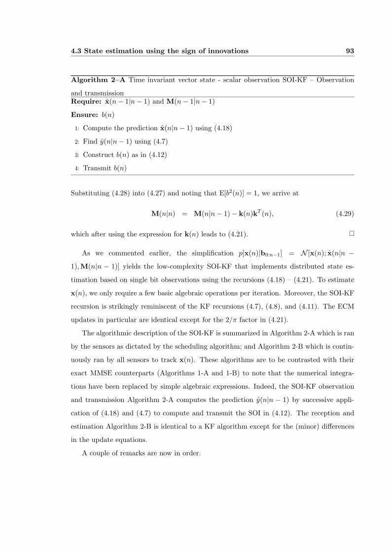
4.3 State estimation using the sign of innovations 93
Algorithm 2–A Time invariant vector state - scalar observation SOI-KF – Observation
and transmissionRequire: x(n− 1|n− 1) and M(n− 1|n− 1)
Ensure: b(n)
1: Compute the prediction x(n|n− 1) using (4.18)
2: Find y(n|n− 1) using (4.7)
3: Construct b(n) as in (4.12)
4: Transmit b(n)
Substituting (4.28) into (4.27) and noting that E[b2(n)] = 1, we arrive at
M(n|n) = M(n|n− 1)− k(n)kT (n), (4.29)
which after using the expression for k(n) leads to (4.21).
As we commented earlier, the simplification p[x(n)|b0:n−1] = N [x(n); x(n|n −1),M(n|n − 1)] yields the low-complexity SOI-KF that implements distributed state es-
timation based on single bit observations using the recursions (4.18) – (4.21). To estimate
x(n), we only require a few basic algebraic operations per iteration. Moreover, the SOI-KF
recursion is strikingly reminiscent of the KF recursions (4.7), (4.8), and (4.11). The ECM
updates in particular are identical except for the 2/π factor in (4.21).
The algorithmic description of the SOI-KF is summarized in Algorithm 2-A which is ran
by the sensors as dictated by the scheduling algorithm; and Algorithm 2-B which is contin-
uously ran by all sensors to track x(n). These algorithms are to be contrasted with their
exact MMSE counterparts (Algorithms 1-A and 1-B) to note that the numerical integra-
tions have been replaced by simple algebraic expressions. Indeed, the SOI-KF observation
and transmission Algorithm 2-A computes the prediction y(n|n − 1) by successive appli-
cation of (4.18) and (4.7) to compute and transmit the SOI in (4.12). The reception and
estimation Algorithm 2-B is identical to a KF algorithm except for the (minor) differences
in the update equations.
A couple of remarks are now in order.

4.3 State estimation using the sign of innovations 94
Algorithm 2–B Time invariant vector state - scalar observation SOI-KF – Reception and
estimationRequire: prior estimate x(−1| − 1) and ECM M(−1| − 1)
1: for n = 0 to ∞ do {repeat for the life of the network}2: Compute x(n|n− 1) and M(n|n− 1) using (4.18) and (4.19)
3: Receive b(n)
4: Compute x(n|n) and M(n|n) using (4.20) and (4.21)
5: end for
Remark 4.2 It is possible to express the SOI-KF corrector in (4.20) in a form that exem-
plifies its link with the KF corrector in (4.11). Indeed, if we define the SOI-KF innovation
as
b(n) :=√
(2/π) [hT (n)M(n|n− 1)h(n) + σ2v(n)] b(n), (4.30)
we can re-write the SOI-KF corrector as
x(n|n) = x(n|n− 1) +M(n|n− 1)h(n)
hT (n)M(n|n− 1)h(n) + σ2v(n)
b(n). (4.31)
Note that (4.31) is identical to (4.11) if we replace b(n) ↔ y(n). Moreover, note that the
units of b(n) and y(n) are the same, and that E[b(n)] = E[y(n)] = 0. Even more interesting
[c.f. (4.11) and (4.32)],
E[b2(n)] = (2/π)[hT (n)M(n|n− 1)h(n) + σ2
v(n)]
= (2/π)E[y2(n)] (4.32)
which explains the relationship between the ECM corrections for the KF in (4.11) and for
the SOI-KF in (4.21). The difference between (4.11) and (4.31) is that in the SOI-KF the
magnitude of the correction at each step is determined by the magnitude of E[b2(n)] and it
is the same regardless of how large or small the actual innovation y(n) is.
Remark 4.3 As σ2v → ∞, the Gaussian tail function Q[±hT [x(n|n− 1)− x(n)]σv] con-
verges uniformly to 1/2, and consequently p[x(n)|b0:n] converges uniformly to a normal
distribution. Thus, the assumption p[x(n)|b0:n−1] = N [x(n); x(n|n− 1),M(n|n− 1)] holds
asymptotically as σ2v →∞.

4.4 Vector state - vector observation case 95
4.4 Vector state - vector observation case
The method for addressing the general vector state - vector observation model defined
by (4.4) is to modify the problem so that we can apply Proposition 4.2. The idea is to
whiten the observations so that we can re-write the problem as a sequence of vector state -
scalar observation problems. To this end, we define the observation y0(n) := C−1/2v (n)y(n)
to obtain [c.f. (4.4)]
y0(n) = C−1/2v (n)H(n)x(n) + C−1/2
v (n)v(n) := H0(n)x(n) + v0(n), (4.33)
where, E[v0(n)vT0 (n)] = I. For future reference, we write y0(n) := [y0(n, 1), . . . , y0(n,M)],
v0(n) := [v0(n, 1), . . . , v0(n,M)] and H0(n) := [h0(n, 1), . . . ,h0(n,M)]T that allows us to
write (4.33) componentwise as:
y0(n,m) = hT0 (n,m)x(n) + v0(n,m), m ∈ [1, M ], (4.34)
where the observation noise variance is σ2v0
:= E[v20(n,m)] = 1.
Eq. (4.34) has the same form as (4.9) in the sense that the state x(n) is a vector
but the observation y0(n,m) is scalar. Mimicking the treatment in Section 4.3, we define
b(n, 1 : m) := [b(n, 1), . . . , b(n,m)]T and introduce the MMSE estimator
x(n|n− 1,m) = E[x(n)|b0:n−1,b(n, 1 : m)], (4.35)
which is the MMSE estimator based on past messages and the first m components of the
current message. We adopt the convention x(n|n − 1, 0) = x(n|n − 1), and note that
x(n|n− 1,M) = x(n|n) with x(n|n− 1) as defined in (4.7) and x(n|n) as defined in (4.6).
From (4.35), we obtain the MMSE predictor of y0(n,m) as [c.f. (4.34) and (4.35)]
y0(n,m|n− 1,m− 1) := E[y0(n,m)|b0:n−1,b(n, 1 : m− 1)]
= hT0 (n,m)x(n|n− 1,m− 1). (4.36)
And from (4.36), we define the SOI observations for the vector state - vector observation
problem as
b(n,m) := sign[y0(n,m)− y0(n, m|n− 1,m− 1)], m ∈ [1, M ]. (4.37)
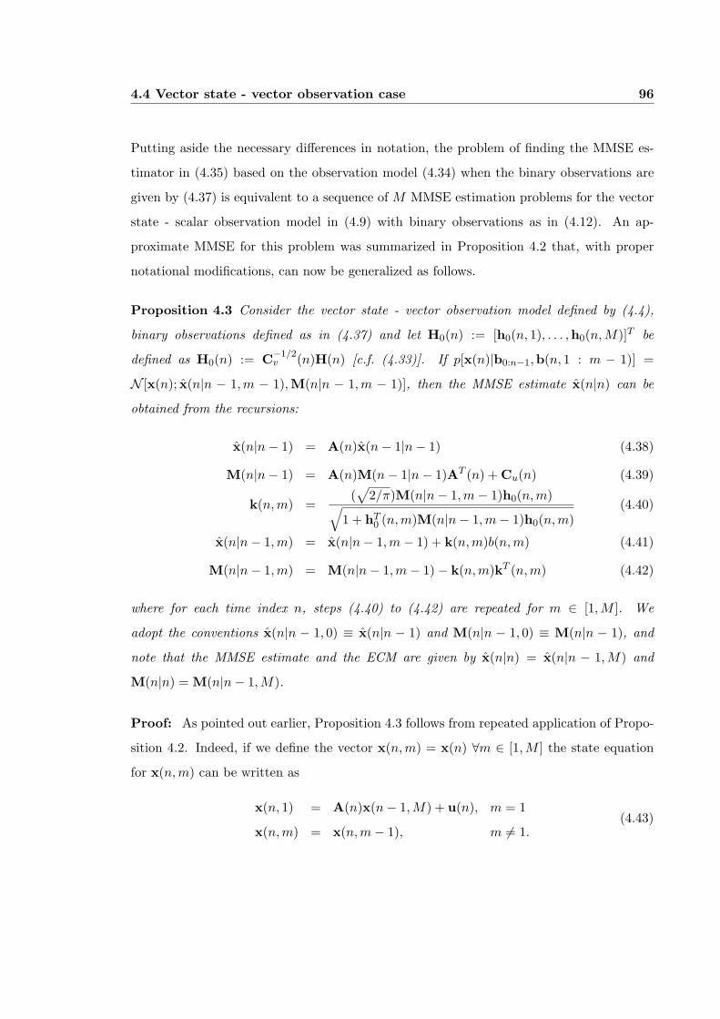
4.4 Vector state - vector observation case 96
Putting aside the necessary differences in notation, the problem of finding the MMSE es-
timator in (4.35) based on the observation model (4.34) when the binary observations are
given by (4.37) is equivalent to a sequence of M MMSE estimation problems for the vector
state - scalar observation model in (4.9) with binary observations as in (4.12). An ap-
proximate MMSE for this problem was summarized in Proposition 4.2 that, with proper
notational modifications, can now be generalized as follows.
Proposition 4.3 Consider the vector state - vector observation model defined by (4.4),
binary observations defined as in (4.37) and let H0(n) := [h0(n, 1), . . . ,h0(n,M)]T be
defined as H0(n) := C−1/2v (n)H(n) [c.f. (4.33)]. If p[x(n)|b0:n−1,b(n, 1 : m − 1)] =
N [x(n); x(n|n − 1,m − 1),M(n|n − 1,m − 1)], then the MMSE estimate x(n|n) can be
obtained from the recursions:
x(n|n− 1) = A(n)x(n− 1|n− 1) (4.38)
M(n|n− 1) = A(n)M(n− 1|n− 1)AT (n) + Cu(n) (4.39)
k(n,m) =(√
2/π)M(n|n− 1,m− 1)h0(n, m)√1 + hT
0 (n,m)M(n|n− 1,m− 1)h0(n,m)(4.40)
x(n|n− 1,m) = x(n|n− 1,m− 1) + k(n,m)b(n,m) (4.41)
M(n|n− 1,m) = M(n|n− 1,m− 1)− k(n,m)kT (n,m) (4.42)
where for each time index n, steps (4.40) to (4.42) are repeated for m ∈ [1,M ]. We
adopt the conventions x(n|n − 1, 0) ≡ x(n|n − 1) and M(n|n − 1, 0) ≡ M(n|n − 1), and
note that the MMSE estimate and the ECM are given by x(n|n) = x(n|n − 1,M) and
M(n|n) = M(n|n− 1,M).
Proof: As pointed out earlier, Proposition 4.3 follows from repeated application of Propo-
sition 4.2. Indeed, if we define the vector x(n,m) = x(n) ∀m ∈ [1,M ] the state equation
for x(n,m) can be written as
x(n, 1) = A(n)x(n− 1,M) + u(n), m = 1
x(n,m) = x(n,m− 1), m 6= 1.(4.43)

4.4 Vector state - vector observation case 97
On the other hand, the whitened observations can be written as [c.f. (4.34) with x(n) =
x(n,m)]
y0(n, m) = hT0 (n,m)x(n,m) + v0(n,m). (4.44)
Define now the MMSE estimators x(n,m|n − 1,m) := E[x(n,m)|b0:n−1,b(n, 1 : m)]
and x(n,m|n − 1,m − 1) := E[x(n, m)|b0:n−1,b(n, 1 : m − 1)] with corresponding ECM
M(n,m|n − 1,m) and M(n,m|n − 1, m − 1). Applying Proposition 4.2, we obtain the
prediction recursions for m = 1 [c.f. (4.18), (4.19), and (4.43)]
x(n, 1|n− 1, 0) = A(n)x(n− 1,M |n− 1, 0)
M(n, 1|n− 1, 0) = A(n)M(n− 1,M |n− 1, 0)AT (n) + Cu(n), (4.45)
and for m ∈ [2,M ] [c.f. (4.18), (4.19), and (4.43)]
x(n,m|n− 1,m− 1) = x(n,m− 1|n− 1,m− 1)
M(n,m|n− 1,m− 1) = M(n,m− 1|n− 1,m− 1). (4.46)
From Proposition 4.2, we also obtain the correction recursions [c.f. (4.20), (4.21), and (4.44)]
k(n,m) =(√
2/π)M(n,m|n− 1,m− 1)h0(n,m)√1 + hT
0 (n,m)M(n,m|n− 1, m− 1)h0(n,m)
x(n,m|n− 1,m) = x(n,m|n− 1,m− 1) + k(n,m)b(n,m)
M(n,m|n− 1,m) = M(n,m|n− 1,m− 1)− k(n,m)kT (n,m). (4.47)
But note that since x(n,m) = x(n) for m ∈ [1,M ], we have that x(n,m|n − 1,m) =
x(n|n − 1,m) and x(n, m|n − 1,m − 1) = x(n|n − 1,m − 1); and likewise for the ECMs:
M(n,m|n − 1, m) = M(n|n − 1,m) and M(n,m|n − 1,m − 1) = M(n|n − 1,m − 1). To
obtain (4.38) and (4.39), it suffices to substitute the latter into (4.45). To obtain (4.40) –
(4.42), we simply make these same substitutions in (4.47) after plugging (4.46) into (4.47).
The algorithmic description of the SOI-KF is summarized in Algorithms 3-A and 3-
B. Algorithm 3-A is ran at the sensors when the scheduling algorithm dictates that it is
their turn to transmit an observation. When this happens, the sensor runs the predictor

4.5 Performance analysis 98
Algorithm 3–A SOI-KF – Observation and transmissionRequire: x(n− 1|n− 1) and M(n− 1|n− 1)
Ensure: s(n)
1: Compute x(n|n− 1) and M(n|n− 1) using (4.38) and (4.39).
2: y0(n) := C−1/2v (n)y(n) and H0(n) := C−1/2
v (n)H(n)
3: for m = 1 to M do
4: Compute y(n,m|n− 1,m− 1) using (4.36)
5: Compute b(n,m) using (4.37)
6: Compute k(n, m), x(n|n− 1,m), and M(n|n− 1,m) using (4.40) , (4.41) and (4.42)
7: end for
8: Transmit b(n) = [b(n, 1), . . . , b(n,M)]
using (4.38) and (4.39) (step 1) and whitens the observation y(n) (step 2). Subsequently,
it recursively computes partial MMSE estimators via (4.36) and (4.40) – (4.42) in order to
obtain the binary observations b(n, m) by means of (4.37). When this process is complete,
the message b(n) is transmitted. Interestingly enough, when the observations are scalar,
Algorithm 3-A amounts to sequential application of steps 1, 2, 4-6 and 8; which is, of course,
equivalent to Algorithm 2-A.
Algorithm 3-B is continuously ran by the sensors to estimate the state x(n). At each
time slot n we compute the predictors along with H0(n) and move on to process the received
message b(n). Processing of b(n) entails recursive application of (4.40) – (4.42) for the M
entries of b(n). After this process is complete, we obtain the MMSE estimate x(n|n).
4.5 Performance analysis
By definition, any MMSE estimator minimizes the trace of the corresponding ECM. Thus,
to the extent that the approximation p[x(n)|b0:n−1] = N [x(n); x(n|n − 1),M(n|n − 1)] is
accurate enough, the SOI-KF in Proposition 4.2 is optimum in the sense of minimizing
tr[M(n|n)] and tr[M(n|n− 1)]. However, this optimality does not provide any insight with
respect to the performance of the SOI-KF relative to the MMSE based on the original

4.5 Performance analysis 99
Algorithm 3–B SOI-KF – Reception and estimationRequire: prior estimate x(−1| − 1) and ECM M(−1| − 1)
1: for n = 0 to ∞ do {repeat for the life of the network}2: Compute x(n|n− 1) and M(n|n− 1) using (4.38) and (4.39).
3: H0(n) := C−1/2v (n)H(n)
4: Receive b(n)
5: for m = 1 to M do
6: Compute k(n, m), x(n|n−1,m), and M(n|n−1,m) using (4.40) , (4.41) and (4.42)
7: end for
8: x(n|n) = x(n|n− 1,M), M(n|n) = M(n|n− 1,M)
9: end for
observations which are used by the clairvoyant KF in (4.7), (4.8), and (4.11). In this
section, we compare tr[M(n|n)] and tr[M(n|n− 1)] for the SOI-KF with tr[MK(n|n)] and
tr[MK(n|n− 1)] reserved to denote the corresponding quantities for the KF.
To simplify notation, define M(n) := M(n|n−1). Interestingly, M(n) is independent of
the observations b0:n, and regardless of the data we can find M(n) by solving the discrete-
time Ricatti equation that is obtained by substituting the expression for M(n|n) in (4.21)
into the ECM update for M(n + 1|n) := M(n + 1) in (4.19),
M(n + 1) = A(n + 1)M(n)AT (n + 1) + Cu(n + 1) (4.48)
− (2/π)A(n + 1)M(n)h(n)hT (n)M(n)AT (n + 1)hT (n)M(n)h(n) + σ2
v(n).
Likewise, upon defining MK(n) := MK(n|n− 1), we obtain the discrete-time Ricatti equa-
tion for the clairvoyant KF [c.f. (4.8) and (4.11)]
MK(n + 1) = A(n + 1)MK(n)AT (n + 1) + Cu(n + 1) (4.49)
− A(n + 1)MK(n)h(n)hT (n)MK(n)AT (n + 1)hT (n)MK(n)h(n) + σ2
v(n).
Notice that (4.48) and (4.49) differ only by the (2/π) factor in the numerator of the ra-
tio in (4.48). A possible performance comparison could be to solve the difference equa-
tions (4.48) and (4.49) for specific models and compare tr[M(n)] with tr[MK(n)]. However,

4.5 Performance analysis 100
better insight can be gained by recalling the underlying continuous-time model, for which
we start with the following definition.
Definition 4.1 Consider the continuous-time model (4.1) – (4.2) and a family of corre-
sponding discrete-time models (4.4) parameterized by Ts. Let M(Ts; n|n) and M(Ts; n|n−1)
be the ECM of the filtered and predicted estimates of the SOI-KF in Proposition 4.2 when
sampling period Ts is used in (4.4). Then, the continuous-time ECM Mc(t) is defined as
Mc(t) := Mc(nTs) := limTs→0
M(Ts; n|n) = limTs→0
M(Ts; n|n− 1). (4.50)
An equivalent definition can be written for the clairvoyant KF whose continuous-time ECM
will be denoted MKc (t) [26]. In general, the continuous-time MSE is easier to analyze but
at the same time more general since, being independent of the sampling time, it provides
insights about the fundamental properties of the problem. Moreover, it is well known
that [26]
tr[M(Ts;n|n)] ≤ tr[Mc(nTs)] ≤ tr[M(Ts; n|n− 1)], ∀Ts. (4.51)
Eq. (4.51) reveals that the continuous-time MSE, tr[Mc(t)], serves as an upper (lower)
bound for tr[M(Ts;n|n)] (tr[M(Ts; n|n − 1)]). The continuous-time ECM Mc(t) can be
obtained by solving a continuous-time Ricatti equation as we show in the next proposition.
Proposition 4.4 For the SOI-KF introduced in Proposition 4.2, consider the continuous-
time ECM Mc(t) given by Definition 4.1. Then Mc(t) can be obtained as the solution of
the differential equation,
Mc(t) = Ac(t)Mc(t)+Mc(t)ATc (t)+Cuc(t)−Mc(t)hc(t)
[π
2σ2
vc(t)
]−1hT
c (t)Mc(t). (4.52)
Proof: Consider a neighborhood around t := nTs. To establish (4.52), it suffices to
subtract M(n) from both sides of (4.48), divide by Ts and let Ts → 0. Indeed, the limit of
the left hand side of (4.48) is
L := limTs→0
M(n + 1)−M(n)Ts
= limTs→0
Mc[(n + 1)Ts]−M(nTs)Ts
= Mc(t), (4.53)

4.5 Performance analysis 101
where the first equality follows from the definition of Mc(nTs) in (4.50) and in the second
equality we used the definition of derivative and set t := nTs. In the right hand side, we
start with the limit
R1 := limTs→0
A(n + 1)M(n)AT (n + 1)−M(n)Ts
= limTs→0
Φ[(n + 1)Ts, nTs]Mc(t)ΦT [(n + 1)Ts, nTs]−Mc(t)Ts
, (4.54)
where in the second equality we used the definitions of A(n + 1) := Φ[(n + 1)Ts, nTs] and
Mc(t) = Mc(nTs) in (4.50). But since Φ[(n + 1)Ts, nTs] = I + Ac(nTs)Ts + o(Ts), we find
R1 = limTs→0
Ts[Ac(t)Mc(t) + Mc(t)ATc (t)] + T 2
s Ac(t)Mc(t)ATc (t) + o(Ts)
Ts
= Ac(t)Mc(t) + Mc(t)ATc (t). (4.55)
Consider now the variance of the driving input whose limit is
R2 := limTs→0
Cu(n + 1)Ts
= limTs→0
1Ts
∫ nTs
(n−1)Ts
Φ(nTs, τ)Cuc(τ)ΦT (nTs, τ)dτ = Cuc(t), (4.56)
where in obtaining the first equality we used the definition of Cu(n+1). To obtain the last
equality we applied the mean value theorem and wrote Φ(nTs, τ) = I+Ac(nTs)(τ −nTs)+
o(τ − nTs).
For the remaining term in the right hand side of (4.48), we define the limit
R3 := limTs→0
(2/π)A(n + 1)M(n)h(n)hT (n)M(n)AT (n + 1)TshT (n)M(n)h(n) + Tsσ2
v(n)
= limTs→0
(2/π)Ac(t)Mc(t)h(t)hT (t)Mc(t)AT (t)TshT (t)Mc(t)h(t) + σ2
vc(t)
=(2/π)Ac(t)Mc(t)h(t)hT (t)Mc(t)AT (t)
σ2vc
(t), (4.57)
where in the second step the key substitution is σ2v(n) = σ2
vc(t)/Ts, and we also used the fact
that limTs→0 A(n + 1) = Ac(t), limTs→0 h(n) = hc(t) and the definition of Mc(t) in (4.50).
Finally, note that according to (4.48) and the definitions of L, Rj we have that L =∑3
j=1Rj . Combining this with the limit expressions in (4.53), (4.55), (4.56) and (4.57), we
obtain (4.52) after rearranging terms.
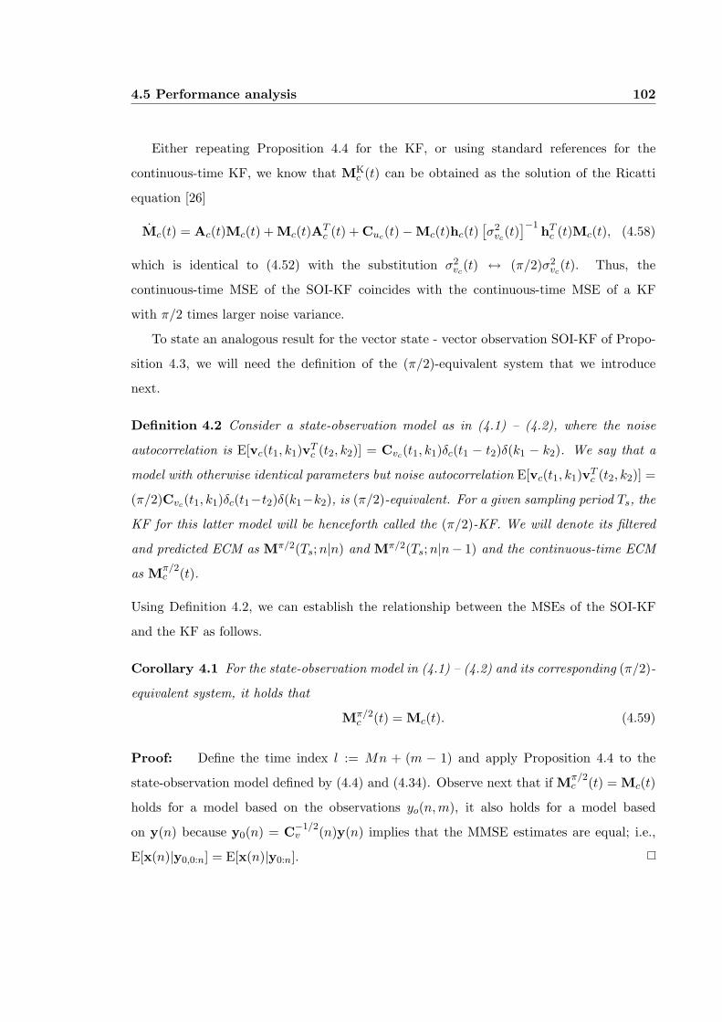
4.5 Performance analysis 102
Either repeating Proposition 4.4 for the KF, or using standard references for the
continuous-time KF, we know that MKc (t) can be obtained as the solution of the Ricatti
equation [26]
Mc(t) = Ac(t)Mc(t) + Mc(t)ATc (t) + Cuc(t)−Mc(t)hc(t)
[σ2
vc(t)
]−1 hTc (t)Mc(t), (4.58)
which is identical to (4.52) with the substitution σ2vc
(t) ↔ (π/2)σ2vc
(t). Thus, the
continuous-time MSE of the SOI-KF coincides with the continuous-time MSE of a KF
with π/2 times larger noise variance.
To state an analogous result for the vector state - vector observation SOI-KF of Propo-
sition 4.3, we will need the definition of the (π/2)-equivalent system that we introduce
next.
Definition 4.2 Consider a state-observation model as in (4.1) – (4.2), where the noise
autocorrelation is E[vc(t1, k1)vTc (t2, k2)] = Cvc(t1, k1)δc(t1 − t2)δ(k1 − k2). We say that a
model with otherwise identical parameters but noise autocorrelation E[vc(t1, k1)vTc (t2, k2)] =
(π/2)Cvc(t1, k1)δc(t1−t2)δ(k1−k2), is (π/2)-equivalent. For a given sampling period Ts, the
KF for this latter model will be henceforth called the (π/2)-KF. We will denote its filtered
and predicted ECM as Mπ/2(Ts; n|n) and Mπ/2(Ts; n|n− 1) and the continuous-time ECM
as Mπ/2c (t).
Using Definition 4.2, we can establish the relationship between the MSEs of the SOI-KF
and the KF as follows.
Corollary 4.1 For the state-observation model in (4.1) – (4.2) and its corresponding (π/2)-
equivalent system, it holds that
Mπ/2c (t) = Mc(t). (4.59)
Proof: Define the time index l := Mn + (m − 1) and apply Proposition 4.4 to the
state-observation model defined by (4.4) and (4.34). Observe next that if Mπ/2c (t) = Mc(t)
holds for a model based on the observations yo(n,m), it also holds for a model based
on y(n) because y0(n) = C−1/2v (n)y(n) implies that the MMSE estimates are equal; i.e.,
E[x(n)|y0,0:n] = E[x(n)|y0:n].

4.6 Simulations 103
1 2 3 4 5 6 7 8
0.75
0.8
0.85
0.9
0.95
1
SOI−KF
time(s)
MS
E
Ts = 2s
Ts = 0.5s
Ts = 0.2s
continuous time
Figure 4.3: The MSEs, tr[M(Ts;n|n)] of the estimator and tr[M(Ts;n|n−1)] of the predictor
converge to the continuous-time MSE tr[Mc(nTs)] as Ts decreases (Ac(t) = I, hc(t) =
[1, 2]T , Cuc(t) = I, and σ2vc
(t) = 1).
Corollary 4.1 establishes that the MSE of the SOI-KF is closely related to the MSE
of the (π/2)-KF, since as Ts → 0 the MSEs of these two filters are equal. For a par-
ticular example, Fig. 4.3 depicts tr[M(Ts; n|n − 1)] and tr[M(Ts; n|n)] for different values
of Ts illustrating how the gap between these two MSEs narrows as Ts decreases, eventu-
ally converging to tr[Mc(nTs)]. Fig. 4.4 compares the KF, the SOI-KF and the (π/2)-KF
for two representative sampling periods Ts. Note that for large Ts, tr[Mπ/2(Ts; n|n)] and
tr[M(Ts;n|n)] are not equal (bottom); but as Ts decreases, these two quantities eventually
coincide (top). It is is also worth noting that tr[Mc(nTs)] = tr[Mπ/2c (nTs)] is a valid upper
bound for tr[M(Ts;n|n)]. We finally stress that the gap between the KF and the SOI-KF
is small even for moderate values of Ts.
4.6 Simulations
The SOI-KF can be applied in a number of situations. Consider for instance measuring e.g.,
room temperature with a WSN. A common state propagation model is the zero-acceleration

4.6 Simulations 104
1 2 3 4 5 6 7 8 9 100.6
0.7
0.8
0.9
1
Sampling time Ts = 1s
time(s)
MS
E
1 1.1 1.2 1.3 1.4 1.5 1.6 1.7 1.8 1.9 20.78
0.8
0.82
0.84
0.86
Sampling time Ts = 0.05
time(s)
MS
E
disc. time KFdisc. time SOI−KFdiscr. time SOI−eq.cont. time KFcont. time SOI−KF
Figure 4.4: The MSE tr[M(Ts; n|n)] of the SOI-KF and the MSE tr[Mπ/2(Ts; n|n)] of the
(π/2)-KF are indistinguishable for small Ts; as Ts increases there is a noticeable but still
small difference. The penalty with respect to tr[MK(Ts; n|n)] is small for moderate Ts
(Ac(t) = I, hc(t) = [1, 2]T , Cuc(t) = I, and σvc(t) = 1).

4.6 Simulations 105
5 10 15 20 25 301.5
2
2.5
3
3.5
4
Ts = 0.5 s
time (s)
tr [
M(n
|n)
] ( o K
2 )
SOI−KF, theoreticalEq. KF, theoreticalSOI−KF, empiricalEq. KF, empirical
10 20 30 40 50 60 70
2
4
6
8
10
Ts = 2 s
time (s)
tr [
M(n
|n)
] (
o K2 )
Figure 4.5: SOI-KF compared with the (π/2)-KF. The filtered MSEs of the two filters are
indistinguishable for small Ts, but as Ts becomes large, the (π/2)-KF is not a good predictor
of the SOI-KF’s performance (β1 = 0.1, β2 = 0.2, σ2u = 1 and σ2
v = 1).
model
xc(t) :=
T (t)
T (t)
=
0 1
0 0
T (t)
T (t)
+
0
1
u(t) := Acxc(t) + uc(t) (4.60)
where T (t) is the room’s temperature, and T (t) and T (t) denote first and second derivatives.
Consistent with u(t) having variance σ2u, the driving input’s covariance matrix is Cuc(t) =
σ2u[0, 1]T [0, 1].
Sensor Sk measures the temperature, but due to thermal inertia the observations are
given by
y(t) = T (t)− βkT (t) + v(t) (4.61)
with βk a sensor dependent constant and σ2vc
(t) = σ2v denoting the noise variance. For
simplicity, we further assume that there are only two sensors that alternate in transmitting
their observations.
Simulations for this problem are depicted in Figs. 4.5 and 4.6, where we can see that
the theoretical MSE curves found as the solution of the corresponding Ricatti equations
4.6 Simulations 106
5 10 15 20 25 301.5
2
2.5
3
3.5
4
Ts = 0.5 s
time (s)
tr [
M(n
|n)
] (
o K2 )
SOI−KF, theoreticalKF, theoreticalSOI−KF, empiricalKF, empirical
10 20 30 40 50 60 70
2
4
6
8
10
Ts = 2 s
time (s)
tr [
M(n
|n)
] ( o K
2 )
Figure 4.6: SOI-KF compared with KF: even for moderate values of Ts, the performance
penalty is small (β1 = 0.1, β2 = 0.2, σ2u = 1 and σ2
v = 1).
closely match the empirical results. In Fig. 4.5, we compare the SOI-KF with the (π/2)-
KF for different sampling periods Ts. While for small Ts these two filters yield indeed
indistinguishable performance (top), as Ts increases there is a noticeable gap between them
(bottom). On the other hand, by inspecting the comparison between SOI-KF and KF in
Fig. 4.6, we deduce that even for relatively large sampling intervals, the MSE penalty paid
for quantizing to a single bit per sensor is small.
4.6.1 Target tracking with SOI-EKF
Target tracking based on distance only measurements is a typical problem in bandwidth-
constrained distributed estimation with WSNs (see e.g., [2,11]) for which a variation of the
SOI-KF appears to be particularly attractive. Consider K sensors randomly and uniformly
deployed in a square region of 2L × 2L meters and suppose that sensor positions {xk}Kk=1
are known.
The WSN is deployed to track the position x(n) := [x1(n), x2(n)]T of a target, whose
state model accounts for x(n) and the velocity v(n) := [v1(n), v2(n)]T , but not for the

4.6 Simulations 107
acceleration that is modelled as a random quantity. Under these assumptions, we obtain
the state equation [14]
x(n)
v(n)
=
1 0 Ts 0
0 1 0 Ts
0 0 1 0
0 0 0 1
x(n− 1)
v(n− 1)
+
T 2s /2 0
0 T 2s /2
Ts 0
0 Ts
u(n), (4.62)
where Ts is the sampling period and the random vector u(n) ∈ R2 is zero-mean white
Gaussian; i.e., p(u(n)) = N (u(n);0; σ2uI). The sensors gather information about their
distance to the target by measuring the received power of a pilot signal following the path-
loss model
yk(n) = α log ‖x(n)− xk‖+ v(n), (4.63)
with α ≥ 2 a constant, ‖x(n)− xk‖ denoting the distance between the target and Sk, and
v(n) the observation noise with distribution p(v(n)) = N (v(n); 0; σ2v).
Mimicking an extended (E)KF approach, we linearize (4.63) in a neighborhood of x(n|n−1) to obtain
yk(n)− y0k(n) ≈ hT (n)x(n) + v(n), (4.64)
where h(n) := αx(n|n− 1)/‖x(n|n− 1)− xk‖2 and y0k(n) is an explicit function of α,
x(n|n− 1) and xk.
The approximate model in (4.62) - (4.64) is of the form (4.4) and we can apply the SOI-
KF outlined in Algorithms 3-A and 3-B to track the target’s position x(n). This procedure
amounts to the implementation of an extended SOI-(E)KF which is a low communication
cost version of the EKF.
The results of simulating this setup are depicted in Figs. 4.7 and 4.8, where we see that
the SOI-KF succeeds in tracking the target with distance error for the position estimates of
less than 10 meters (m). While this accuracy is just a result of the specific parameters of the
experiment, the important point here is that the clairvoyant EKF and the SOI-EKF yield
almost identical performance even when the former relies on analog-amplitude observations
and the SOI-EKF on the transmission of a single bit per sensor.

4.6 Simulations 108
0 200 400 600 800 1000 1200 1400 1600 1800 20000
200
400
600
800
1000
1200
1400
position x1 (m)
posi
tion
x 2 (m
)
SensorsTargetEKFSOI−EKF
Figure 4.7: Target tracking with EKF and SOI-EKF yield almost identical estimates. The
scheduling algorithm works in cycles of duration T . At the beginning of the cycle, we
schedule the sensor Sk closest to the estimate x(n|n − 1), next the second closest and so
on until we complete the cycle (T = 4, Ts = 1s, L = 2km, K = 100, α = 3.4 σu = 0.2m,
σv = 1).
0 100 200 300 400 500 6000
2
4
6
8
10
12
14
16
18
20
time (s)
dist
ance
from
targ
et to
est
imat
e (m
)
EKFSOI−EKF
Figure 4.8: Standard deviation of the estimates in Fig. 4.7 are in the order of 5m-10m for
both filters.

4.7 Appendix – Proof of (4.20) 109
4.7 Appendix – Proof of (4.20)
To simplify notation, we will drop the time argument to write h = h(n) and σ2v = σ2
v(n).
Due to the symmetry of the problem, it suffices to consider the case b(n) = 1. Start with
the change of variables x(n) := x(n)− x(n|n− 1), so that we can write (4.26) as
x(n|n) = x(n|n− 1) + 2∫
Rp
x(n)exp
[−12 x
T (n)M−1(n|n− 1)x(n)]
(2π)p/2 det1/2[M(n|n− 1)]Q
[−hT x(n)
σv
]dx(n).
(4.65)
Introduce a second change of variables z := M−1/2(n|n − 1)x(n), and also let g :=
M1/2(n|n− 1)h to obtain
x(n|n) = x(n|n− 1) +2M1/2(n|n− 1)
(2π)p/2
∫
Rp
z exp[−zTz
2
]Q
[−gT z
σv
]dz, (4.66)
where we recall that dz = det[M−1/2(n|n − 1)]dx(n) = dx(n)/ det[M1/2(n|n − 1)]. Define
the integral l := [2/(2π)p/2]∫Rp x(n) exp
[−uTu/2]Q
[−gTu/σv
]du = [l1, . . . , lp]T , that we
can express componentwise as
lk =2
(2π)p/2
∫
Rp−1
exp
[−zT
−kz−k
2
]∫
Rzk exp
[−z2
k
2
] ∫ ∞
−[gT−ku−k+gkuk]
exp[− v2
2σ2v
]√
2π σv
dz−kdzkdv,
(4.67)
where we used the definition Q[−gTz/σv] :=∫∞−gT z[1/(
√2πσv)] exp
[−v2/2σ2v
]dv, in-
troduced the notations z−k := [z1, . . . , zk−1, zk+1, . . . , zp]T and g−k := [g1, . . . , gk−1,
gk+1, . . . , gp]T , and separated the exponent as zTz = zT−kz−k + z2
k.
We can now observe that zk exp[−z2
k/2]
= −(∂/∂zk) exp[−z2
k/2]
and interchange the
last two integrals in (4.67) to obtain
lk =2sign(gk)(2π)p/2
∫ ∞
Rp−1
exp
[−zT
−kz−k
2
]∫
R
exp[− v2
2σ2v
]√
2π σv
∫ ∞
−[gT−ku−k+v]/gk
∂
∂zkexp
[−z2
k
2
]dz−kdvdzk
=2
(2π)(p+1)/2σv
∫
Rp−1
exp
[−zT
−kz−k
2
]∫
Rexp
[− v2
2σ2v
−(gT−ku−k + v)2
2g2k
]dz−kdv, (4.68)
with the last equality following from the fundamental theorem of calculus. We can further

4.7 Appendix – Proof of (4.20) 110
rearrange terms in (4.68) and interchange the integrals to arrive at
lk =2sign(gk)
(2π)(p+1)/2σv
∫
Rexp
[−v2
2
(1σ2
v
+1g2k
)](4.69)
∫
Rp−1
exp
[−1
2
(zT−k
(I +
g−kgT−k
g2k
)z−k −
2gT−kz−kv
g2k
)]dvdz−k.
Consider now the quadratic form in the exponent of the second integral, and let us sum-
marize a number of properties about this form in the following lemma:
Lemma 4.1 If we define the matrix C−1 := I + g−kgT−k/g2
k, it holds that:
(a) the inverse of C−1 is given by C = I− g−kgT−k/g
Tg
(b) the determinant of C−1 is det(C−1) = gTg/g2k
(c) the quadratic form in the exponent of the second integral in (4.69) can be written as
zT−kC
−1z−k −2gT−kz−kv
g2k
= (z−k − µ)TC−1(z−k − µ)− v2gT−kg−k
g2kg
Tg(4.70)
with µ :=(−v/g2
k
)C−1g−k.
Proof: Statement (a) follows from the matrix inversion lemma, which can be proved by
verifying that CC−1 = I. To prove (b), let w be an eigenvector of C−1; being an eigenvector
of C−1, w must satisfy
C−1w = w +g−kgT
−kwg2k
= λww, (4.71)
for some constant λw. Note that (4.71) is satisfied by w1 = g−k with λw1 = 1+gT−kg−k/g2
k,
and by any wj perpendicular to g−k such that gT−kwj = 0 with λwj = 1. Since the
determinant can be expressed as the product of the eigenvalues, we have
det(C−1) =p−1∏
j=1
λwj =
(1 +
gT−kg−k
g2k
)p−1∏
j=2
λwj . (4.72)
But the dimension of the subspace perpendicular to g−k is p − 2, and thus,∏p−1
j=2 λj = 1.
Statement (b) is obtained by simply rearranging terms.
To prove (c), expand the right hand side and verify that the equality is indeed true.

4.7 Appendix – Proof of (4.20) 111
Using Lemma 4.1-(c), we can rewrite (4.69) as
lk =2sign(gk)
(2π)(p+1)/2σv
∫
Rexp
[−v2
2
(1σ2
v
+1g2k
− gT−kg−k
g2kg
Tg
)]dv (4.73)
×∫
Rp−1
exp[−1
2(z−k − µ)T C−1 (z−k − µ)
]dz−k,
where the two integrals are independent. The second integral is the integral of a
(p − 1)-dimensional Gaussian distribution over Rp−1 which regardless of µ is equal to
(2π)(p−1)/2 det1/2(C); given that det(C) is given by the inverse of the expression in
Lemma 4.1-(b), we obtain
∫
Rp−1
exp[−1
2(z−k − µ)T C−1 (z−k − µ)
]dz−k = (2π)(p−1)/2
(g2k
gTg
)1/2
. (4.74)
The first integral in (4.73) is the integral of a Gaussian bell over R and is thus given by√
2π times the standard deviation:
∫
Rexp
[−v2
2
(1σ2
v
+1g2k
− gT−kg−k
g2kg
Tg
)]dv =
√2π
(σ2
vgTg
gTg + σ2v
)1/2
. (4.75)
Substituting (4.74) and (4.75) into (4.73), we obtain
lk =
√2/π√
gTg + σ2v
gk. (4.76)
Placing the components of l given by (4.76) into (4.66) yields the expression
x(n|n) = x(n|n− 1) +
√2/π√
gTg + σ2v
M1/2(n|n− 1)g. (4.77)
Recalling that g := M1/2(n|n−1)h, (4.26) follows for b(n) = 1. For b(n) = −1, the opposite
result follows from symmetry.

112
Chapter 5
Conclusions and Future Work
We were motivated by the need to reduce communication costs in a wireless sensor network
deployed to estimate parameters of interest in a decentralized fashion. Throughout the
dissertation we considered different situations with a flow towards more pragmatic signal
models. We have shown that for deterministic parameter estimation as well as for state
estimation of dynamic stochastic processes it is possible to find estimators whose complexity
and performance are similar to that of corresponding clairvoyant estimators based on the
transmission of the original analog-amplitude observations.
We started in Chapter 2 by studying the fundamental properties of the problem by look-
ing at deterministic mean-location estimation in additive white Gaussian noise (AWGN).
Under the strict bandwidth constraint of just 1 bit per sensor, we introduced a class of
MLEs that attain a variance close to the sample mean estimator’s variance when the noise
variance is comparable with the dynamic range of the parameter to be estimated. This
class of estimators is well suited for low-to-medium SNR problems. Relaxing the band-
width constraint, we also constructed the best possible estimator for a given total number
of bits. This led us to the per bit CRLB which revealed a trade off between reducing the
quantization step and making room for transmitting more independent observations. A
general rule of thumb is that selecting a quantization step equal to the noise variance is
good enough for most practical situations. Finally, by comparing this last MLE with the
QSME we deduced that for high SNR problems even the least complex scheme performs

Chapter 5. Conclusions and Future Work 113
close to the optimum. Consequently, bandwidth-constrained distributed estimation is not
a relevant problem in such cases and the QSME should be used for its low complexity.
We have also studied implementation issues, and established that all the MLE problems
we considered are convex. Consequently, they can be efficiently solved and their numerical
convergence is assured.
Though the noise was assumed Gaussian throughout Chapter 2, it is worth noting that
Theorem 2.1 and Propositions 2.1, 2.3 and 2.4-(b) are valid for any noise distribution,
Propositions 2.2, and 2.4-(a) only require a log-concave distribution. This suggested that
these results may hold in more pragmatic scenarios and motivated Chapter 3 where we
studied the extent to which the low performance penalty and low complexity claims of
Chapter 2 extended to situations of practical significance.
Thus, in Chapter 3 we developed parameter estimators for realistic signal models and
derived their fundamental variance limits under bandwidth constraints. The latter were
adhered to by quantizing each sensor’s observation to one or a few bits. By jointly accounting
for the unique quantization-estimation tradeoffs present, these bit(s) per sensor were first
used to derive distributed maximum likelihood estimators (MLEs) for scalar mean-location
parameters in the presence of generally non-Gaussian noise when the noise pdf is completely
known; subsequently, when the pdf is known except for a number of unknown parameters;
and finally, when the noise pdf is unknown. The unknown pdf case was tackled through a
non-parametric estimator of the unknown complementary cumulative distribution function
based on quantized (binary) observations. In all three cases, the resulting estimators turned
out to exhibit comparable variances that can come surprisingly close to the variance of the
clairvoyant estimator which relies on unquantized observations. This happens when the SNR
capturing both quantization and noise effects assumes low-to-moderate values. Analogous
claims were established for practical generalizations that were pursued in the multivariate
and colored noise cases for distributed estimation of vector parameters under bandwidth
constraints. Therein, MLEs were formed via numerical search but the log-likelihoods were
proved to be concave thus ensuring fast convergence to the unique global maximum. A
motivating application was also considered reinforcing the conclusion that in low-cost-per-

5.1 Future research 114
node wireless sensor networks, distributed parameter estimation based even on a single bit
per observation is possible with minimal increase in estimation variance.
The minimal increase in estimation variance in low-to-moderate SNR values suggests an
inherent match with state estimation of dynamic stochastic processes in which we can use
the predicted estimate to quantize the current observation. This was pursued in Chapter 4.
Relying on the sign of innovations (SOI), we considered the problem of distributed
state estimation in the context of wireless sensor networks. The binary SOI data destroy
the linearity of the problem and lead to prohibitively complex MMSE state estimation.
This motivated an approximation leading to the SOI-Kalman filter (KF) which offers an
approximate MMSE estimator whose complexity and performance are very close to that of
a KF even when the latter is based on the original (analog-amplitude) observations and the
SOI-KF is based on the transmission of a single bit per observation. Relating the discrete-
time KF and SOI-KF with the underlying continuous-time physical process monitored by
the WSN, we established that the MSE of the SOI-KF coincides with the MSE of a KF
applied to an otherwise equivalent system model with π/2 larger noise covariance matrix.
This result was established in the limit as the sampling period becomes arbitrarily small;
but practical simulations confirmed its validity even for moderate-size sampling intervals.
The SOI-KF was applied to a motivating application entailing temperature monitoring and
to the canonical target tracking problem based on distance-only measurements. In both
cases, we corroborated that at low communication cost the SOI-KF and the SOI-EKF yield
estimates that are indistinguishable from the estimates of the clairvoyant KF and EKF for
all practical purposes.
5.1 Future research
This thesis studied the intertwining between quantization and estimation arising in dis-
tributed sensor networks. Building on our results we devise a number of future research
topics; in this section we describe two topics that we are actively pursuing at the moment.

5.1 Future research 115
5.1.1 Maximum a posteriori estimation with binary observations
In Chapters 2 and 3 we considered given some form of prior information in the form of a
weight function or a parameter dynamic range suggesting a connection with maximum a
posteriori (MAP) estimation. Viewing the deterministic parameter θ as a random one with
prior distribution W (θ), the log-distribution after observing the vector of binary observa-
tions is given by,
LMAP (θ) = L(θ) + ln[W (θ)], (5.1)
with L(θ) given by (2.14). The MAP estimator is defined as θMAP = arg max[LMAP (θ)].
Note that being L(θ) ∝ N , it holds that LMAP (θ) → L(θ) when N → ∞, and ac-
cordingly both estimators coincide asymptotically. In particular, the average variance of
the MAP estimator converges to the average variance of the MLE, and minimization of
BW (τ ,ρ) as defined in (2.19) yields the asymptotically optimum MAP estimator (as well
as the asymptotically optimal MLE). Also worth mentioning is that if the prior distribu-
tion W (θ) is log-concave then the likelihood in (5.1) is concave. This is the case for many
distributions including the Gaussian and the Uniform one.
In any event, note that most of the conclusions in Chapters 2 and 3 appear to be
generalizable to MAP estimation. However, different from MLE, MAP estimators exploit
the prior information in computing the estimate.
5.1.2 Extensions of the SOI-KF
The use of SOI can be extended to different setups. As we pursued the SOI-EKF, one can
envision similar combinations with the (SOI-)UKF and the (SOI-)PF in which we trade
complexity for performance in highly non-linear state estimation problems. The SOI-KF
sheds light on this problem from two angles. On the one hand it suggests that a SOI-UKF
(SOI-PF) may have a small performance penalty with respect to the corresponding UKF
(PF) based on the analog-amplitude observations. On the other hand one can envision a
situation in which the UKF (PF) is used to track the model non-linearities and the SOI-KF
is invoked to take care of the quantization non-linearities.

5.1 Future research 116
A second generalization is a multi-bit version of the SOI-KF in which the kth bit of a
quantized observation is defined as the SOI relative to the estimator based on the previous
k − 1 bits. In both cases, the goal is to effect distributed state estimation with low-cost
communications.
117
Bibliography
[1] M. Abdallah and H. Papadopoulos, “Sequential signal encoding and estimation fordistributed sensor networks,” in Proc. of the International Conference on Acoustics,Speech, and Signal Processing, vol. 4, pp. 2577–2580, Salt Lake City, Utah, May 2001.
[2] J. Aslam, Z. Butler, F. Constantin, V. Crespi, G. Cybenko, and D. Rus, “Trackinga moving object with a binary sensor network,” in Proc. of the 1st Intl. Conf. onEmbedded Networked Sensor Systems, pp. 150–161, Los Angeles, CA, USA, 2003.
[3] E. Ayanoglu, “On Optimal Quantization of Noisy Sources,” IEEE Transactions onInformation Theory, vol. 36, pp. 1450–1452, Nov. 1990.
[4] B. Beferull-Lozano, R. L. Konsbruck, and M. Vetterli, “Rate-Distortion problem forphysics based distributed sensing,” in Proc. of the Intnl, Conf. on Acoustics, Speech,and Signal Processing, vol. 3, pp. 913–916, Montreal, Canada, May 2004.
[5] D. Blatt and A. Hero, “Distributed maximum likelihood estimation for sensor net-works,” in Proc. of the Intl, Conf. on Acoustics, Speech, and Signal Processing, vol. 3,pp. 929–932, Montreal, Canada, May 2004.
[6] S. Boyd and L. Vandenberghe, Convex Optimization. Cambridge University Press,2004.
[7] T. H. Chung, V. Gupta, B. Hassibi, J. Burdick, and R. M. Murray, “Scheduling fordistributed sensor networks with single sensor measurement per time step,” in Proc.of the Intl. Conf. on Robotics and Automation, vol. 1, pp. 187–192, New Orleans, LA,April 26 - May 1, 2004.
[8] R. Curry, W. Vandervelde, and J. Potter, “Nonlinear Estimation with Quantized Mea-surements – PCM, Predictive Quantization, and Data Compression,” IEEE Transac-tions on Information Theory, vol. 16, pp. 152–161, March 1970.

BIBLIOGRAPHY 118
[9] G. Dahlquist and A. Bjorck, Numerical Methods. Prentice-Hall Series in AutomaticComputation, 1974.
[10] P. Djuric, J. Kotecha, J. Zhang, Y. Huang, T. Ghirmai, M. Bugallo, and J. Miguez,“Particle filtering,” IEEE Signal Processing Magazine, vol. 20, pp. 19–38, Sep. 2003.
[11] P. Djuric, M. Vemula, and M. Bugallo, “Tracking with particle filtering in tertiarywireless sensor networks,” in Proc. of Intl. Conf. on Acoustics, Speech and Signal Pro-cessing, vol. 4, pp. 757–760, Philadelphia, PA, USA, March 19-23, 2005.
[12] E. Ertin, R. Moses, and L. Potter, “Network parameter estimation with detectionfailures,” in Proc. of the Intl, Conf. on Acoustics, Speech, and Signal Processing, vol. 2,pp. 273–276, Montreal, Canada, May 2004.
[13] J. Gubner, “Distributed Estimation and Quantization,” IEEE Transactions on Infor-mation Theory, vol. 39, pp. 1456–1459, 1993.
[14] F. Gustafsson, F. Gunnarsson, N. Bergman, U. Forssell, J. Jansson, R. Karlsson, andP.-J. Nordlund, “Particle filters for positioning, navigation, and tracking,” IEEE Trans-actions on Signal Processing, vol. 50, pp. 425–437, Feb. 2002.
[15] S. Julier and J. Uhlmann, “Unscented filtering and nonlinear estimation,” Proceedingsof the IEEE, vol. 92, pp. 401–422, March 2004.
[16] S. M. Kay, Fundamentals of Statistical Signal Processing - Estimation Theory. PrenticeHall, 1993.
[17] S. M. Kay, Fundamentals of Statistical Signal Processing - Detection Theory. PrenticeHall, 1998.
[18] J. Kotecha and P. Djuric, “Gaussian particle filtering,” IEEE Transactions on SignalProcessing, vol. 51, pp. 2602–2612, Oct. 2003.
[19] S. Kumar, F. Zao, and D. Shepherd, eds., Special issue on collaborative informationprocessing, vol. 19 of IEEE Signal Processing Magazine, March 2002.
[20] W. Lam and A. Reibman, “Quantizer design for decentralized systems with commu-nication constraints,” IEEE Transactions on Communications, vol. 41, pp. 1602–1605,Aug. 1993.
[21] Z.-Q. Luo, “An isotropic universal decentralized estimation scheme for a bandwidthconstrained ad hoc sensor network,” IEEE Journal on Selected Areas in Communica-tions, vol. 23, pp. 735–744, April 2005.

BIBLIOGRAPHY 119
[22] Z.-Q. Luo, “Universal Decentralized Estimation in a Bandwidth Constrained SensorNetwork,” IEEE Transactions on Information Theory, 2005 (to appear). available athttp://www.ece.umn.edu/users/luozq/recent work.html.
[23] Z.-Q. Luo and J.-J. Xiao, “Decentralized estimation in an inhomogeneous sensing envi-ronment,” IEEE Transactions on Information Theory, May 2004 (submitted). availableat http://www.ece.umn.edu/users/luozq/recent work.html.
[24] Z. Luo, M. Gastpar, J. Liu, and A. Swami, eds., Special Issue on Distributed SignalProcessing in Sensor Networks, IEEE Signal Processing Magazine, (to appear) 2006.
[25] A. Mainwaring, D. Culler, J. Polastre, R. Szewczyk, and J. Anderson, “Wireless sensornetworks for habitat monitoring,” in Proc. of the 1st ACM Intl. Workshop on WirelessSensor Networks and Applications, vol. 3, pp. 88–97, Atlanta, Georgia, 2002.
[26] P. S. Maybeck, Stochastic Models, Estimation and Control – Vol.1. Academic Press,first ed., 1979.
[27] R. D. Nowak, “Distributed EM algorithms for density estimation and clustering insensor networks,” IEEE Transactions on Signal Processing, vol. 51, pp. 2245–2253,August 2002.
[28] H. Papadopoulos, G. Wornell, and A. Oppenheim, “Sequential signal encoding fromnoisy measurements using quantizers with dynamic bias control,” IEEE Transactionson Information Theory, vol. 47, pp. 978–1002, 2001.
[29] H. C. Papadopoulos, “Efficient Digital Encoding and Estimation of Noisy Signals,”Ph.D. Thesis, Massachusets Institute of Technology, May 1998.
[30] B. Porat, Digital processing of random signals. Prentice Hall, 1994.
[31] S. S. Pradhan, J. Kusuma, and K. Ramchandran, “Distributed compression in a densemicrosensor network,” IEEE Signal Processing Magazine, vol. 19, pp. 51–60, March2002.
[32] J. G. Proakis, Digital Communications. McGraw-Hill Higher Education, fourth ed.,2001.
[33] M. G. Rabbat and R. D. Nowak, “Decentralized source localization and tracking,” inProc. of the Intl. Conf. on Acoustics, Speech, and Signal Processing, vol. 3, pp. 921–924,Montreal, Canada, May 2004.

BIBLIOGRAPHY 120
[34] A. Ribeiro and G. B. Giannakis, “Non-parametric distributed quantization-estimationusing wireless sensor networks,” in Proc. of Intl. Conference on Acoustics, Speech andSignal Processing, vol. 4, pp. 61–64, Philadelphia, PA, March 18-23, 2005.
[35] A. Ribeiro and G. B. Giannakis, “Distributed Kalman Filtering Based onSeverely Quantized WSN Data,” in Proc. of IEEE Workshop on Statistical Sig-nal Processing, Bordeaux, France, July 17-20, 2005 (to appear). Available athttp://www.ece.umn.edu/users/aribeiro/research/pubs.html.
[36] A. Ribeiro and G. B. Giannakis, “Distributed quantization-estimation us-ing wireless sensor networks,” in Proc. of Intl. Conference on Commu-nications, Seoul, Korea, May 16-20, 2005 (to appear). Available athttp://www.ece.umn.edu/users/aribeiro/research/pubs.html.
[37] A. Ribeiro and G. B. Giannakis, “Bandwidth-Constrained Distributed Es-timation for Wireless Sensor Networks, Part I: Gaussian Case,” IEEETransactions on Signal Processing, 2006 (to appear). available athttp://www.ece.umn.edu/users/aribeiro/research/pubs.html.
[38] A. Ribeiro and G. B. Giannakis, “Bandwidth-Constrained Distributed Es-timation for Wireless Sensor Networks, Part II: Unknown pdf,” IEEETransactions on Signal Processing, 2006 (to appear). available athttp://www.ece.umn.edu/users/aribeiro/research/pubs.html.
[39] A. Ribeiro, G. B. Giannakis, and S. Roumeliotis, “SOI-KF: Distributed KalmanFiltering with Low-Cost Communications using the Sign Of Innovations,” IEEETransactions on Signal Processing, August 2005 (submitted). available athttp://www.ece.umn.edu/users/aribeiro/research/pubs.html.
[40] A. Ribeiro and G. B. Giannakis, “Distributed estimation in Gaussian noise forbandwidth-constrained wireless sensor networks,” in Proc. of 38th Asilomar Conf. onSignals, Systems, & Comp., vol. 2, pp. 1407–1411, Monterrey, CA, USA, November7-10, 2004.
[41] S. Servetto, R. Knopp, A. Ephremides, S. Verdu, S. Wicker, and L. Cimini, “GuestEditorial: Fundamental performance limits of wireless sensor networks,” IEEE Journalon Selected Areas on Communications, vol. 22, pp. 961–965, August 2004.
[42] J. F. Sturm, “Using Sedumi 1.02, a Matlab toolbox for optimization over symmetriccones,” available at http://fewcal.kub.nl/sturm/software/sedumi.html.

BIBLIOGRAPHY 121
[43] Y. Sung, L. Tong, and A. Swami, “Asymptotic locally optimal detector for large-scalesensor networks under the Poisson regime,” in Proc. of the Intnl, Conf. on Acoustics,Speech, and Signal Processing, vol. 2, pp. 1077–1080, Montreal, Canada, May 2004.
[44] P. K. Varshney, Distributed Detection and Data Fusion. Springer-Verlag, 1997.
[45] D. Williamson, “Finite Wordlength Design of Digital Kalman Filters for State Estima-tion,” IEEE Transactions on Automatic Control, vol. 30, pp. 930–939, Oct. 1985.