university of Çukurova institute of …library.cu.edu.tr/tezler/6415.pdf · i would like to thank...

UNIVERSITY OF ÇUKUROVA INSTITUTE OF NATURAL AND APPLIED SCIENCES

MSc THESIS Nilgün ÖZGENÇ DEVELOPMENT OF AN INTERACTIVE CONSTRUCTIVE SOLID GEOMETRY MODELING TOOL

DEPARTMENT OF ELECTRICAL AND ELECTRONICS ENGINEERING

ADANA, 2007

ÇUKUROVA ÜNİVERSİTESİ

FEN BİLİMLERİ ENSTİTÜSÜ

DEVELOPMENT OF AN INTERACTIVE CONSTRUCTIVE SOLID GEOMETRY MODELING TOOL

Nilgün ÖZGENÇ

YÜKSEK LİSANS TEZİ

ELEKTRİK ELEKTRONİK MÜHENDİSLİĞİ ANABİLİM DALI

Bu tez 17 / 08 / 2007 Tarihinde Aşağıdaki Jüri Üyeleri Tarafından Oybirliği

/ Oyçokluğu İle Kabul Edilmiştir.

İmza............……… İmza............……… İmza............………

Yrd.Doç.Dr. Ulus ÇEVİK Yrd.Doç.Dr. Mustafa GÖK Yrd.Doç.Dr. Mutlu AVCI

DANIŞMAN ÜYE ÜYE

Bu tez Enstitümüz Elektrik Elektronik Mühendisliği Anabilim Dalında hazırlanmıştır.

Kod No: Prof.Dr.Aziz ERTUNÇ Enstitü Müdürü İmza-Mühür

Not: Bu tezde kullanılan özgün ve başka kaynaktan yapılan bildirişlerin, çizelge, şekil ve fotoğrafların kaynak gösterilmeden kullanımı, 5846 sayılı Fikir ve Sanat Eserleri Kanunundaki hükümlere tabidir.

I

ABSTRACT

MSc THESIS

DEVELOPMENT OF AN INTERACTIVE CONSTRUCTIVE SOLID GEOMETRY MODELING TOOL

Nilgün ÖZGENÇ

DEPARTMENT OF ELECTRICAL AND ELECTRONICS ENGINEERING

INSTITUTE OF NATURAL AND APPLIED SCIENCES

UNIVERSITY OF ÇUKUROVA

Supervisor: Assist. Prof. Dr. Ulus ÇEVİK Year: August 2007, Pages: 60 Jury: Assist. Prof. Dr. Ulus ÇEVİK Assist. Prof. Dr. Mustafa GÖK Assist. Prof. Dr. Mutlu AVCI

Constructive Solid Geometry (CSG) is one of the techniques in solid modeling. CSG is commonly used in 3D computer graphics, CAD, CAM, CAE, robotics, animation, medical imaging, and reverse engineering of design process. In this study, an interactive CSG modeling tool has been developed for interactively creating constructive solid geometry model graphical data in half-space format. Especially, massively parallel graphics systems, called ‘pixel-based’, which generate CSG scenes in real-time, accept scenes in terms of half-spaces. Unbounded planes divide space into half-spaces. By combining half-spaces through regularized set operations, new complex solid models are obtained. This work is motivated by the need of obtaining the half-space CSG representation data of a solid model interactively. Using the tool, graphical data exchange data of various formats can be created for further use. The new CSG format that includes the CSG structure of the model together with its half-space primitives can be used in pixel-based processors, reverse engineering of the design, animation, and robotics because of its hierarchical structure.

Key Words: modeling, solid modeling, constructive solid geometry, half-spaces, pixel-based graphical processor

II

ÖZ

YÜKSEK LİSANS TEZİ

ETKİLEŞİMLİ YAPISAL KATI GEOMETRİ MODELLEME ARACI GELİŞTİRME

Nilgün ÖZGENÇ

ELEKTRİK ELEKTRONİK MÜHENDİSLİĞİ ANABİLİM DALI

FEN BİLİMLERİ ENSTİTÜSÜ

ÇUKUROVA ÜNİVERSİTESİ

Danışman: Yrd. Doç. Dr. Ulus ÇEVİK Yıl: Ağustos 2007 Sayfa: 60 Jüri: Yrd. Doç. Dr. Ulus ÇEVİK Yrd. Doç. Dr. Mustafa GÖK Yrd. Doç. Dr. Mutlu AVCI

Yapısal Katı Geometri (YKG) katı modellemede kullanılan bir tekniktir. YKG

3D bilgisayar grafiklerinde, bilgisayar destekli tasarım, üretim ve mühendislik, robotik, medikal görüntüleme, bilgisayar animasyonu ve tasarım işleminin tersine mühendisliği alanlarında yoğunlukla kullanılır. Bu çalışmada YKG modelin yarı-uzay tabanlı grafik verisini etkileşimli olarak üretmek amacı ile bir katı modelleme aracı geliştirilmiştir. Pixel tabanlı grafik işlemcilerinde YKG modelini oluşturan basit bileşenler yarı-uzaylarla tanımlanır. Booelan set işlemleri kullanılarak yarı-uzaylarlar ile tanımlanan basit katı bileşenlerden yeni karmaşık katı modeller elde edilebilir. Bu çalışmada YKG metodu ile oluşturulan bir modelin, YKG ve yarı-uzay tanımlı basit bileşenlerinin grafiksel verisinin etkileşimli olarak elde edilmesi amaçlanmıştır. Bu formatta üretilen modelin grafiksel verisi hiyerarşik yapısı dolayısıyla; pixel-tabanlı grafik işlemleyicilerinde, modelin tersine mühendisliğinde, animasyon ve robotik algoritmalarında kullanılabilir. Anahtar Kelimeler: Modelleme, katı modelleme, yapısal katı geometri, yarı-uzay, pixel-tabanlı grafik işlemleyicleri

III

ACKNOWLEDGEMENTS

The subject of this thesis was suggested by my supervisor, Assist. Prof. Dr.

Ulus ÇEVİK to whom I would like to express my heartfelt thanks for his supervision,

guidance, encouragements, and extremely useful suggestions throughout this thesis.

I would like to express my appreciation to Prof. Dr. Süleyman GÜNGÖR,

Head of the Department of Electrical and Electronics Engineering, providing

materials and study environment.

I would like to thank Prof. Dr. Mehmet TÜMAY, Head of the Computer

Engineering Department, for his support.

I would like to thank my parents who, throughout my whole life, have always

supported and encouraged me.

And last but not least, a special thank you to my husband for all his support

through the years and to my daughter for her creative support for creating solid

models and for her patience.

Nilgün ÖZGENÇ

IV

CONTENTS PAGE

ABSTRACT..................................................................................................................I

ÖZ.................................................................................................................................II

ACKNOWLEDGEMENTS........................................................................................III

CONTENTS...............................................................................................................IV

LIST OF FIGURES...................................................................................................VII

LIST OF ABBREVIATIONS...................................................................................VIII

1. INTRODUCTION...................................................................................................1

1.1. Motivation of the Work.....................................................................................4

1.2. Content..............................................................................................................5

2. CONSTRUCTIVE SOLID GEOMETRY................................................................5

2.1. Overview...........................................................................................................5

2.2. Regularized Set Operations…….………………………..................................5

2.3. CSG Tree………...............................................................................................5

2.4. CSG Expression ..............................................................................................7

2.5. Representation of Primitives.............................................................................7

2.5.1. Parametric Primitives..............................................................................7

2.5.2. Boundary Representation........................................................................8

2.5.3. Half-spaces..............................................................................................9

2.6. CSG Algorithms…..........................................................................................10

2.7. CSG Applications............................................................................................11

3. GRAPHICAL DATA INTERCHANGE FORMATS.............................................12

3.1. Overview of 3D Graphics Formats.................................................................12

3.2. General Formats..............................................................................................12

3.2.1. STL Format...........................................................................................12

3.2.2. OBJ Format...........................................................................................13

3.3. Modeler Specific Formats...............................................................................13

3.4. CSG Format....................................................................................................13

4. THE CSG MODELER – CSGMOD.....................................................................15

4.1. The Need for the CSG Modeler.....................................................................15

V

CONTENTS PAGE

4.2. Technical Overview of the Modeler...............................................................15

4.3. Modeling Process ………………………………..........................................15

4.3.1. Representing and Generating Primitives.............................................19

4.3.2. Modifying Primitives...........................................................................20

4.3.3. Generating Compound Solids..............................................................20

4.4. Functional Overview......................................................................................21

4.4.1. Primitive Creation and Modification...................................................22

4.4.2. Compound Construction and Modification.........................................23

4.4.3. Compound Decomposition..................................................................24

4.4.4. Constraint Management.......................................................................24

4.4.5. Applying Transformations...................................................................26

4.4.6. Copying Primitives and Compounds...................................................26

4.4.7. Loading and Saving Solid Models.......................................................27

4.4.8. Exporting Graphical Data to Other Formats........................................29

5. THE CSG GRAPHICAL DATA INTERCHANGE FORMAT..............................30

5.1. Overview.........................................................................................................30

5.2. Boolean Expression Derivation......................................................................31

5.3. Plane Equations Derivation.............................................................................31

5.4. CSG Data with Half-Space Primitives............................................................32

5.5. CSG Data with Boundary Represented Primitives.........................................33

5.6. CSG Data with Depth Values.........................................................................33

6. RESULTS AND DISCUSSIONS..........................................................................36

7. CONCLUSION AND FUTURE WORK..............................................................39

REFERENCES...........................................................................................................41

APPENDIX A: A SAMPLE STL FILE......................................................................42

APPENDIX B: A SAMPLE OBJ FILE......................................................................45

APPENDIX C: THE OBJECT-SPACE CSG ALGORITM........................................48

APPENDIX D: CSG DATA WITH DEPTH VALUES..............................................54

APPENDIX E: THE HIERARCHICAL STRUCTURE OF A SOLID MODEL.......57

VI

CONTENTS PAGE

BIOGRAPHY.............................................................................................................59

LIST OF PUBLICATIONS........................................................................................60

VII

LIST OF FIGURES PAGE Figure 1.1a A traditional display pipeline...................................................................3

Figure 1.1b The CSG renderer.....................................................................................6

Figure 2.1 The CSG Tree of a Sample Model………………………………….…..6

Figure 2.2 The CSG Tree of a Spoon constructed Applying Boolean Operations....6

Figure 2.3 A simple b-rep model constructed using six faces...................................8

Figure 2.4 A vertex boundary model…………………………….............................9

Figure 2.5 Two half-spaces are formed by the plane...............................................10

Figure 4.1 The GUI of the modeler..........................................................................16

Figure 4.2 Application Scene Graph........................................................................17

Figure 4.3 Main panes of the modeler......................................................................22

Figure 4.4 Basic primitives: box, cone, sphere, and cylinder...................................23

Figure 4.5 The construction process of a sample model ..........................................24

Figure 4.6 Surface contact constraint........................................................................25

Figure 4.7 Copy operation........................................................................................27

Figure 4.8 Save operation.........................................................................................28

Figure 4.9 Load operation..........................................................................................28

Figure 5.1 A compound solid constructed from three primitives .............................32

Figure 5.2 Compound2 is constructed from box1 and cylinder1 with a...................35

difference operation

Figure 6.1 The display of STL formatted models on SolidView .............................36

Figure 6.1 The display of OBJ formatted models on DeskArtes View.....................37

Figure 6.2 Some mechanical parts designed with the modeler.................................38

Figure C.1 Intersection possibilities of a polygon and a line in a plane ..................51

Figure C.2 Selecting polygons for output…………………….................................53

Figure E.1 Hierarchic structure of a solid model in the tool.......................................57

VIII

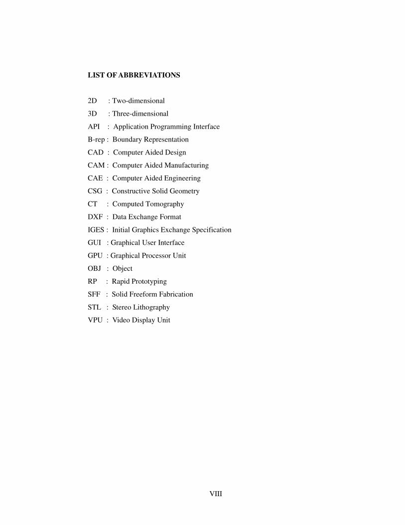
LIST OF ABBREVIATIONS

2D : Two-dimensional

3D : Three-dimensional

API : Application Programming Interface

B-rep : Boundary Representation

CAD : Computer Aided Design

CAM : Computer Aided Manufacturing

CAE : Computer Aided Engineering

CSG : Constructive Solid Geometry

CT : Computed Tomography

DXF : Data Exchange Format

IGES : Initial Graphics Exchange Specification

GUI : Graphical User Interface

GPU : Graphical Processor Unit

OBJ : Object

RP : Rapid Prototyping

SFF : Solid Freeform Fabrication

STL : Stereo Lithography

VPU : Video Display Unit

1. INTRODUCTION Nilgün ÖZGENÇ

1

1. INTRODUCTION

The aim of this thesis is to develop an interactive solid modeler tool that

implements constructive geometry solid modeling method to create solid models and

exports their graphical exchange data for further use. The exported data can be used

in solid modeling, reverse engineering, GPU algorithms, animation and robotics.

A solid is a tree-dimensional shape that can be defined by its exterior and

interior. The interior and exterior of the solid are separated by its boundary. With

solid models, we can compute mass properties such as volume and moments of

inertia; we can check for interference and detect collisions; we can also apply finite

element analysis to calculate stress, and strain for solid models.

There are two main techniques predominate in solid modeling systems today.

The first one is constructive solid geometry (CSG). The other is boundary

representation (b-rep). In general, solid modeling software adopts a dual

representation consisting of CSG and B-rep, where parameters and constraints are

maintained at nodes of CSG trees and the corresponding topologic entities are kept in

a B-rep representation. The boundary representation method represents a solid as a

collection of boundary surfaces. B-rep models are comprised of two parts: topology

and geometry. Topology defines how the surfaces are connected together. The main

topological items are faces, edges, and vertices. Geometry defines where the surfaces

actually are in space. Topology and geometry are strongly linked.

The CSG modeling tool that has been developed in this study is a hybrid

modeler using the constructive solid geometry as a modeling representation and

boundary representation as the internal representation of primitives and compounds

of the final model. It has been developed using Java and Java 3D. It is platform

independent and can be used as a web application.

1.1. Motivation of the Work

CSG modeling approach is used together with other solid modeling

techniques in today’s 3D design and solid modeling packages. Most of the major


2

commercial solid modeling packages currently in distribution (e.g., Pro/ENGINEER

[commonly known as Pro/E], Unigraphics, and SolidWorks etc.) use the boundary

representation (b-rep) as the base approach for solid modeling.

In the literature, some rendering packages (RayShade, POVRay, Blue Moon

Rendering Tools (BMRT), and Radience) used CSG as a solid modeling approach

(Wolfe 1998). Some modeling packages (ALICE, SCED, Breeze Designer, Rhino,

IRIT, and so on) also implemented CSG together with other solid modeling

approaches. EUCLID and BRL-CAD are the solid modelers based on the CSG

modeling approach.

The BRL-CAD package (Anderson and Edwards, 2004) is a powerful CSG

solid modeling system. The package has been developed by the U.S. Army Research

Laboratory since 1979. They have been developing and distributing the BRL-CAD

CSG modeling package for a wide range of military and industrial applications. The

package includes a large collection of tools and utilities including an interactive

geometry editor, ray tracing and generic frame-buffer libraries, a network-distributed

image-processing and signal-processing capability, and an embedded scripting

language. The package runs on the UNIX platform. BRL-CAD has been developed

with C and scripting languages.

Among the solid modelers, none of them exports the CSG data in a simple

half-space format that includes only the model’s CSG structure and its half-space

represented primitives. This study is motivated by the need of obtaining half-space

CSG representation of a solid model interactively. Half-space CSG representations

are generally used in image-based CSG rendering algorithms. The half-space data

was required for studies given in (Çevik, 2004, and Koc, 1999). The half-space CSG

data of the solid models can be used for the simulation process of these studies.

In the study ( Çevik, 2004), an efficient CSG image renderer that is based on

a general Z-buffer hidden-surface removal algorithm with parallel processing of

pixels belonging to object primitives were designed. This renderer can be used for

effective visualization of three-dimensional convex and concave objects. Algorithms,

given in the study, to display a CSG object are based on the comparisons of distances

depth between the viewpoint and surfaces in the scene. The rendering unit named as


3

CSG renderer, whose outlook is given in Figure 1.1 creates convex and concave CSG

object primitives, which are constructed on a plane-by-plane basis. At the input of

this unit are the depths of the planes at the origin of the display space, which

comprise the objects, and their colors in a correct order. The output is the current

view of the scene as intended.

Figure 1.1. (a) A traditional display pipeline. (b) The CSG renderer

The CSG renderer consists of four main components, namely, the tree-

structured depth generator, the pixel processor, the corner bender, and the frame-

buffer. The tree-structured depth generator that accepts the depth of a plane at the

origin, and the differential X and Y increments along the X and Y-axes as the input

evaluates the depth values of the plane at all pixel positions simultaneously on the

display area. The pixel processors manipulate the depth data supplied by the depth

generator to assess which planes will be visible on the display area, comparing the

depths and natures of the planes. The pixel processors process the data in a Bit-Serial

fashion for the sake of parallelism. The corner bender is a serial-to-parallel converter

that is necessary to feed the pixel colors, which have been stored serially, to the VDU

(Video Display Unit). The frame-buffer consists of high-speed RAMs to store the

colors of the scene produced by the pixel processor.


4

In the study, convex and concave objects were defined by their surfaces. A

surface operator, @, was used to mathematically define each surface of the object. In

this notation, the union and the intersection of two objects can be written as follows:

@(A.B)=@(A).B+@(B).A (1.1)

@(A+B)=@(A).!B+@B.!A (1.2)

where . denotes the intersection, + denotes the union operation and ! denotes the

inverse. The difference operation is defined as .!

The developed modeler tool can export the CSG expression in infix form

together with each primitive’s depth values. This data then can be used in the study

that is briefly explained above to form the final CSG object. The format of the

exported data and the data imported to the explained study is explained in Chapter 5

in detail.

1.2. Content

The content of the thesis is arranged as follows: After this introductory

chapter, in Chapter 2, constructive solid geometry concepts (theory and techniques)

are explained in detail. In Chapter 3, graphical data exchange formats are covered. In

Chapter 4, the CSG modeler tool is covered in detail. Firstly, the characteristics of a

solid modeler are defined. Then the technical specifications of the modeler are given.

The modeling process and functionality of the modeler is explained in detail. The

new generalized half-space graphical format data is explained in Chapter 5. In

Chapter 6, the results of this thesis study are discussed. The usage of exported data

formats is illustrated. In Chapter 7, the important conclusions of the study are

explained and the future work topics on the modeler are given.

2. CONSTRUCTIVE SOLID GEOMETRY Nilgün ÖZGENÇ

5

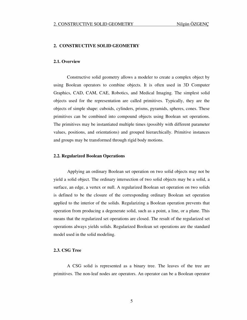
2. CONSTRUCTIVE SOLID GEOMETRY

2.1. Overview

Constructive solid geometry allows a modeler to create a complex object by

using Boolean operators to combine objects. It is often used in 3D Computer

Graphics, CAD, CAM, CAE, Robotics, and Medical Imaging. The simplest solid

objects used for the representation are called primitives. Typically, they are the

objects of simple shape: cuboids, cylinders, prisms, pyramids, spheres, cones. These

primitives can be combined into compound objects using Boolean set operations.

The primitives may be instantiated multiple times (possibly with different parameter

values, positions, and orientations) and grouped hierarchically. Primitive instances

and groups may be transformed through rigid body motions.

2.2. Regularized Boolean Operations

Applying an ordinary Boolean set operation on two solid objects may not be

yield a solid object. The ordinary intersection of two solid objects may be a solid, a

surface, an edge, a vertex or null. A regularized Boolean set operation on two solids

is defined to be the closure of the corresponding ordinary Boolean set operation

applied to the interior of the solids. Regularizing a Boolean operation prevents that

operation from producing a degenerate solid, such as a point, a line, or a plane. This

means that the regularized set operations are closed. The result of the regularized set

operations always yields solids. Regularized Boolean set operations are the standard

model used in the solid modeling.

2.3. CSG Tree

A CSG solid is represented as a binary tree. The leaves of the tree are

primitives. The non-leaf nodes are operators. An operator can be a Boolean operator


6

or, a transformation operator. In Figure 2.1, the CSG tree of a CSG model is shown.

In Figure 2.1, more complex model (a spoon) and its construction tree are shown.

Figure 2.1. The CSG tree of a sample model

Figure 2.2. The CSG tree of a spoon constructed by applying set operations (Laidlaw, Trumbore, Hughes, 1986)


7

2.4. CSG Expression

The CSG expression can be reached by traversing the CGS tree. The CSG

expression for the CSG tree shown in Figure 2.1 can be written as fallows;

(box6Usphere1) U (box5-cylinder5) where U denotes union operation, and - denotes

difference operation.

2.5. Representation of Primitives

The basic primitives that are used to construct the solid model are cubes,

cylinders, spheres, cones and half-spaces. In CSG, primitives can be defined as

parametrically by setting their parameters. Solids are described as combinations of

simple primitives or other solids in a series of Boolean operations.

The constructive solid geometry needs another representation, its internal

representation. The internal representation of the primitives in CSG is generally in

two forms. The first one is the boundary representation that is the commonest

representation in solid modeling. In this representation, the CSG operations (that are

set operations and rigid transformations) are performed on the object space. The

second representation is half-space representation. In half-space representation, the

CSG operations are performed in image space.

2.5.1. Parametric Primitives

Primitives are defined by their parameters. For example, a cylinder can be

defined by its radius and height. The primitives may be instantiated multiple times

(possibly with different parameter values, positions, and orientations) and grouped

hierarchically.


8

2.5.2 Boundary Representation

Boundary (B-Rep) models represent a solid indirectly by a representation of

its bounding surface. A B-Rep solid is represented as a volume contained in a set of

faces together with topological information, which defines the relationships between

the faces. Because B-Rep includes such topological information, a solid is

represented as a closed space in 3D space. The boundary of a solid separates points

inside from points outside of the solid. A very simple B-rep model constructed using

six faces is shown in Figure 2.3.

Boundary represented models are comprised of two parts: topology and

geometry. Topology defines how the surfaces are connected together. The main

topological items are faces, edges, and vertices. Geometry defines where the surfaces

actually are in space. Topology and geometry are strongly linked.

Figure 2.3. A simple B-rep model constructed using six faces

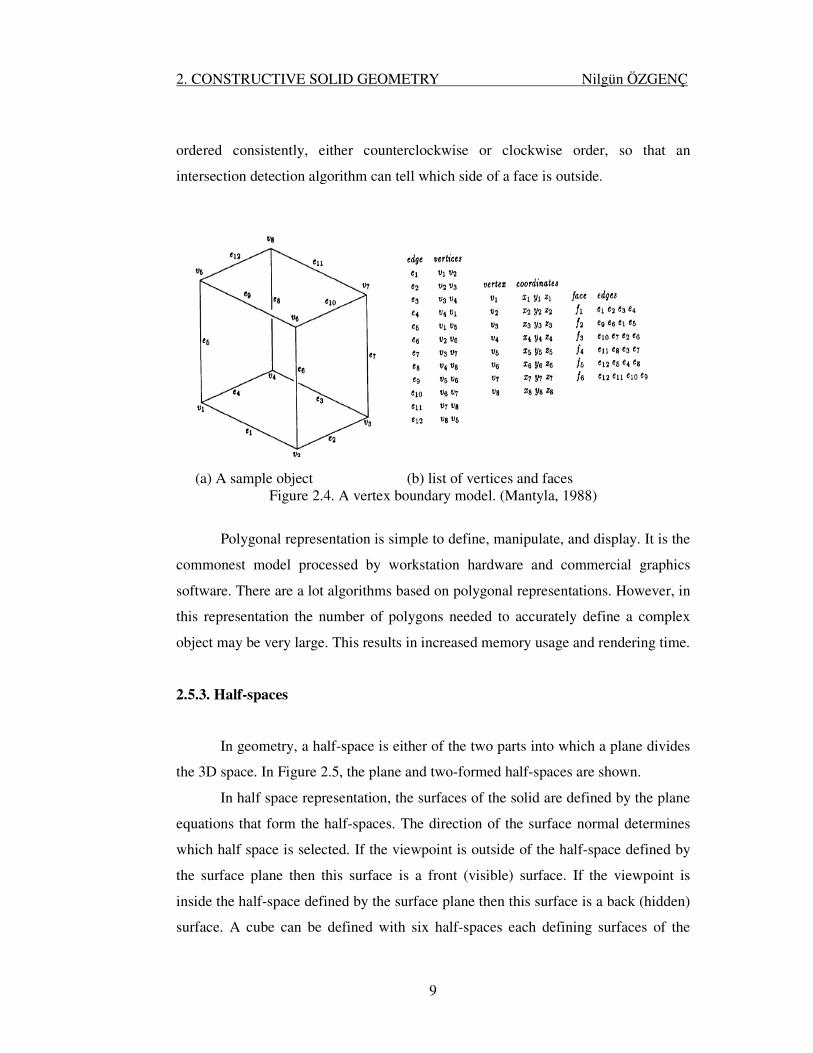
One form of the b-rep is the polygonal representation. Polygonal models are

one of the most commonly encountered representations in computer graphics. The

solid is represented as a connected set of polygons (usually triangles). The simplest

representation of a solid surface is a vertex-based polygonal model consisting of lists

of vertices and polygonal faces, as shown in Figure 2.4 (a). If a face has holes, it has

to be subdivided into a set of simpler polygons with no holes. The Vertex-based

representation has been widely used in many computer graphics file formats. In this

representation vertices are stored in an unordered list of vertices and each face are

stored in an unordered list of faces as shown in Figure 2.4 (b). The vertices must be


9

ordered consistently, either counterclockwise or clockwise order, so that an

intersection detection algorithm can tell which side of a face is outside.

(a) A sample object (b) list of vertices and faces

Figure 2.4. A vertex boundary model. (Mantyla, 1988)

Polygonal representation is simple to define, manipulate, and display. It is the

commonest model processed by workstation hardware and commercial graphics

software. There are a lot algorithms based on polygonal representations. However, in

this representation the number of polygons needed to accurately define a complex

object may be very large. This results in increased memory usage and rendering time.

2.5.3. Half-spaces

In geometry, a half-space is either of the two parts into which a plane divides

the 3D space. In Figure 2.5, the plane and two-formed half-spaces are shown.

In half space representation, the surfaces of the solid are defined by the plane

equations that form the half-spaces. The direction of the surface normal determines

which half space is selected. If the viewpoint is outside of the half-space defined by

the surface plane then this surface is a front (visible) surface. If the viewpoint is

inside the half-space defined by the surface plane then this surface is a back (hidden)

surface. A cube can be defined with six half-spaces each defining surfaces of the


10

cube and the inner of the cube. The half-space represented solids are rendered in

image space. The pixel operations on these solids can be processed in parallel to

shorten the rendering time. This representation is very powerful for animation

purposes because of its parallelism. Since the Boolean set operations are applied in

image-space, the half-space representations also used in rendering algorithms of the

pixel-based graphical processor units.

Figure 2.5. Two half-spaces are formed by a plane.

2.6. CSG Algorithms

There are two approaches for rendering CSG trees. Image-space approach

draws CSG trees directly by performing, view-dependent surface clipping, and

visible surface determination on a per pixel basis. Clipping is performed as a part of

rendering process, and operate on pixels. Image-based CSG algorithms are

algorithms for z-buffer graphics hardware that generate just the image of a CSG

shape without calculating a description of the final object geometry.

Object-space algorithms are performed on object-space and require boundary

evaluation algorithms. The algorithms require an intermediate representation (such as

b-rep). Firstly, boundary representation of the model is evaluated using boundary

evaluation algorithm, and then the polygonal faces of the model are rendered with a

polygon-based renderer. The boundary evaluator algorithm detects intersections


11

between participating solids, computes intersection geometries (intersection points

and curves as well as sub-divided faces) and classifies them using set membership

classification algorithms to determine whether the geometry is in, on, or outside the

final solid defined by the Boolean operation.

The advantage of the image-based approach is that it provides for possibility

of huge parallelism. Each pixel can be processed simultaneously. Because of this

fact, image-based algorithms are faster. In the interactive modeling applications such

as CAD software, the modeling process includes such processes that do not related

with the CSG process directly. These processes do not require the reconstruction of

the model (such as, defining constraints, performing transformations, changing

appearance). In the interactive modelers, these processes are extensively used. These

processes do not require the evaluation of the CSG algorithm. They can be rendered

using an ordinary renderer. In the case of image-based approach, the CSG algorithm

must be evaluated in each case even if the model structure is not changed. Therefore,

the object-space CSG approach based on boundary representation is more relevant

for the interactive modelers. Image-based approach is more effective for applications

where number of restructuring changes is higher than the number of other modeling

changes (such as animation, robotics).

2.7. CSG Applications

Constructive solid geometry has a number of practical uses. It is used in cases

where simple geometric objects are desired, or where mathematical accuracy is

important. The CSG representation is unambiguous and concise. The set operations

are computationally convenient and the rigid motion parameters offer a natural

control of the solid’s shape, position, and orientation. Because of its hierarchical

structure, CSG models can be used in solid modeling, reverse engineering, animation

and robotics.

3. GRAPHICAL DATA INTERCHANGE FORMATS Nilgün ÖZGENÇ

12

3. GRAPHICAL DATA INTERCHANGE FORMATS

3.1. Overview of 3D Graphics Formats

The graphical exchange data for 3D computer graphics are generally

based on polygonal data. All of the solid modeler packages support this kind of data

for both exporting and importing graphics data. In addition, there are some package

specific but again widely used graphical data formats. Many of these formats again

depend on polygonal data together with some other graphical data (texture, light,

material, etc.)

3.2. General Formats

The most common general graphical data exchange formats are STL and

OBJ formats. STL is the standard format for rapid prototyping.

3.2.1. STL Format

The STL format was developed by 3D Systems, Inc., in the 1980s for use

with its StereoLithography Apparatus (SLA). The SLA device produces a physical 3-

D model based on an STL format file. Because of its simplicity, the STL format has

become an industry standard for exchanging 3-D models. Unfortunately, this

simplicity also presents some limitations (Macmains, 2000).

The format consists only of triangles, and each triangle is represented by three

vertices and a surface normal vector. STL files may be either ASCII or binary. The

ASCII format includes the capability of including more than one solid part and an

optional name for each part, while the binary format can only support a single solid

part with no naming. In Appendix A, a sample STL file is documented.


13

3.2.2. OBJ Format

The Wavefront .obj file format is a standard 3D object file format. Object

files are text based files supporting both polygonal and free form geometry (curves

and surfaces).

The OBJ file format supports polygonal data together with free-form curves

and surfaces. Polygons are described in terms of their points, while curves and

surfaces are defined with control points and other information depending on the type

of curve. The format supports rational and non-rational curves, including those based

on Bezier, B-spline, Cardinal (Catmull-Rom splines), and Taylor equations

(WAVEFRONT).

In Appendix B, a more complicated example OBJ file with smooth surfaces

of different types, material assignment, line continuation, and grouping is

demonstrated.

3.3. Modeler Specific Formats

Some other more specific formats are also used (IGES, DWG, DXF, STEP,

WRL, and so on). These formats have more information than polygonal data, such as

texture, color, light, camera position and other CAD related data.

3.4. CSG Format

Half spaces are used as primitive representations of CSG. Half-space data

consists of the equation of the plane that forms the half-space. Unbounded planes

divide space into half-spaces. Complex shaped volumes can be constructed from the

union of collection of these units.

The plane equations is AX + BY + CZ + D = 0 where (A, B, C) is the

outward face normal of the plane and |D| is the perpendicular distance of the plane

from the origin.

There are some software specific half-space and CSG data exporting

formats. For example, IGES have an interface to create BRLCAD CSG format


14

graphical data. However, this data is specific to BRLCAD. It is in the database

structure of the BRLCAD software. It includes the parameters and scripts to create

the CSG model. There is a need for creating a simple and a general half-space

representation data that contains only plane equations data for CSG related studies

and modelers. This type of data is easier to implement. The import interface for this

format data is very simple and easy to code.

4. THE CSG MODELER – CSGMOD Nilgün ÖZGENÇ

15

4. THE CSG MODELER

4.1. The Need for the Modeler

We need an interactive solid modeler tool that can compose a solid model

interactively and export the solid composition data as CSG tree and half-space

primitives. This data was required for studies explained in (Çevik, 2004, Koç, 1999).

The exported data can be used for the simulation process of these studies. The

modeler is a hybrid modeler. The exchange data can also be used by other solid

modelers, in reverse engineering, in GPUs, in animation and robotics.

4.2. Technical Overview of the Modeler

The modeler is a hybrid modeler using CSG as solid model representation

and boundary representation as primitive representation. It is based on CSG

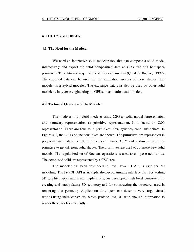
representation. There are four solid primitives: box, cylinder, cone, and sphere. In

Figure 4.1, the GUI and the primitives are shown. The primitives are represented in

polygonal mesh data format. The user can change X, Y and Z dimension of the

primitive to get different solid shapes. The primitives are used to compose new solid

models. The regularized set of Boolean operations is used to compose new solids.

The composed solid are represented by a CSG tree.

The modeler has been developed in Java. Java 3D API is used for 3D

modeling. The Java 3D API is an application-programming interface used for writing

3D graphics applications and applets. It gives developers high-level constructs for

creating and manipulating 3D geometry and for constructing the structures used in

rendering that geometry. Application developers can describe very large virtual

worlds using these constructs, which provide Java 3D with enough information to

render these worlds efficiently.


16

Figure 4.1. GUI of the modeler

Java 3D delivers Java's "write once, run anywhere" benefit to developers of

3D graphics applications. Java 3D is part of the JavaMedia suite of APIs, making it

available on a wide range of platforms. It also integrates well with the Internet

because applications and applets written using the Java 3D API have access to the

entire set of Java classes.

The Java 3D API draws its ideas from existing graphics APIs and from new

technologies. Java 3D's low-level graphics constructs synthesize the best ideas found

in low-level APIs such as Direct3D, OpenGL, QuickDraw3D, and XGL. Similarly,

its higher-level constructs synthesize the best ideas found in several scene graph-

based systems. Java 3D introduces some concepts not commonly considered part of

the graphics environment, such as 3D spatial sound. Java 3D's sound capabilities

help to provide a more immersive experience for the user.


17

Java 3D is an object-oriented API. Applications construct individual graphics

elements as separate objects and connect them together into a treelike structure called

a scene graph. The application manipulates these objects using their predefined

accessor, mutator, and node-linking methods.

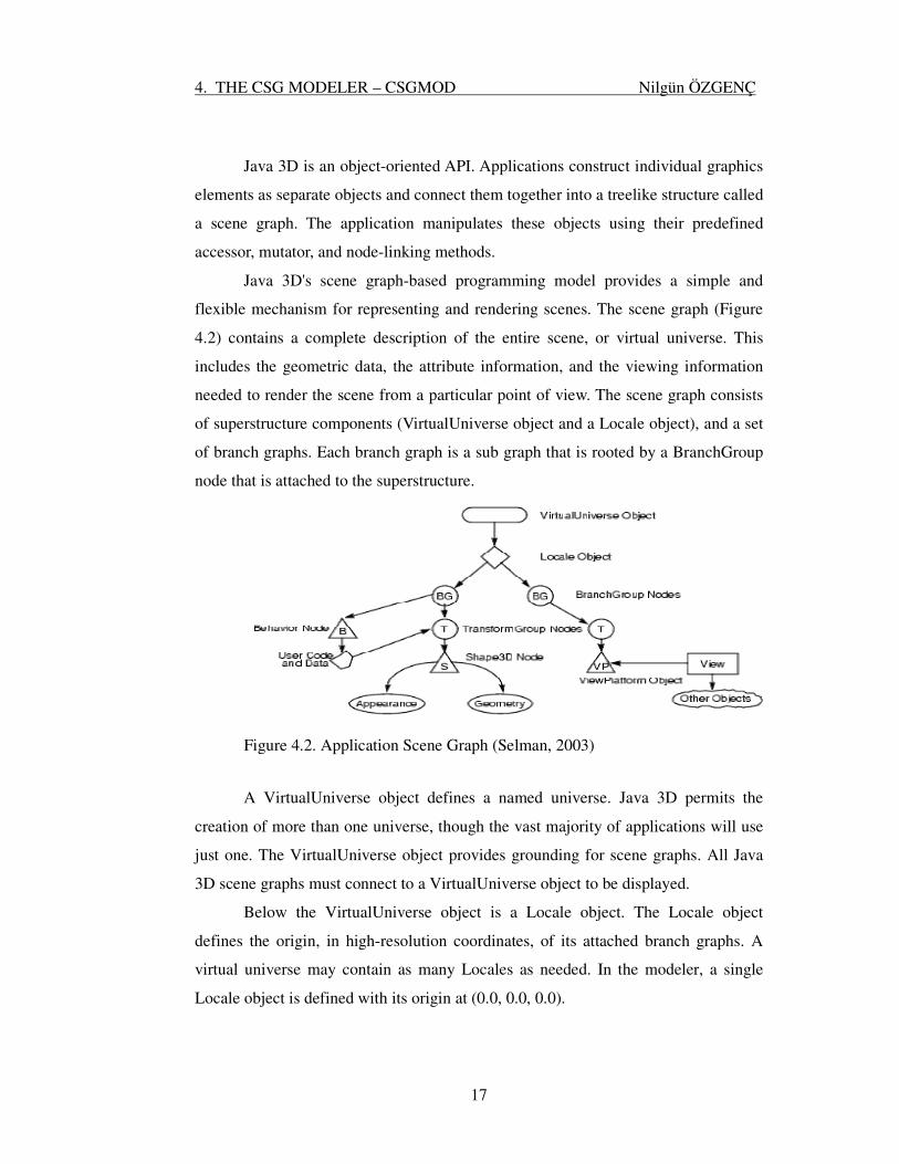
Java 3D's scene graph-based programming model provides a simple and

flexible mechanism for representing and rendering scenes. The scene graph (Figure

4.2) contains a complete description of the entire scene, or virtual universe. This

includes the geometric data, the attribute information, and the viewing information

needed to render the scene from a particular point of view. The scene graph consists

of superstructure components (VirtualUniverse object and a Locale object), and a set

of branch graphs. Each branch graph is a sub graph that is rooted by a BranchGroup

node that is attached to the superstructure.

Figure 4.2. Application Scene Graph (Selman, 2003)

A VirtualUniverse object defines a named universe. Java 3D permits the

creation of more than one universe, though the vast majority of applications will use

just one. The VirtualUniverse object provides grounding for scene graphs. All Java

3D scene graphs must connect to a VirtualUniverse object to be displayed.

Below the VirtualUniverse object is a Locale object. The Locale object

defines the origin, in high-resolution coordinates, of its attached branch graphs. A

virtual universe may contain as many Locales as needed. In the modeler, a single

Locale object is defined with its origin at (0.0, 0.0, 0.0).


18

The scene graph itself starts with the BranchGroup nodes. A BranchGroup

serves as the root of a sub graph, called a branch graph, of the scene graph. Only

BranchGroup objects can attach to Locale objects.

In Figure 4.2, there are two branch graphs and, thus, two BranchGroup nodes.

Attached to the left BranchGroup are two sub graphs. One sub graph consists of a

user-extended Behavior leaf node. The Behavior node contains Java code for

manipulating the transformation matrix associated with the object's geometry.

The other sub graph in this BranchGroup consists of a TransformGroup node

that specifies the position (relative to the Locale), orientation, and scale of the

geometric objects in the virtual universe. A single child, a Shape3D leaf node, refers

to two component objects: a Geometry object and an Appearance object. The

Geometry object describes the geometric shape of a 3D object (a cube in our simple

example). The Appearance object describes the appearance of the geometry (color,

texture, material reflection characteristics, and so forth).

The right BranchGroup has a single sub graph that consists of a

TransformGroup node and a ViewPlatform leaf node. The TransformGroup specifies

the position (relative to the Locale), orientation, and scale of the ViewPlatform. This

transformed ViewPlatform object defines the end user's view within the virtual

universe.

Finally, the ViewPlatform is referenced by a View object that specifies all of

the parameters needed to render the scene from the point of view of the

ViewPlatform. Also referenced by the View object are other objects that contain

information, such as the drawing canvas into which Java 3D renders, the screen that

contains the canvas, and information about the physical environment.

In the modeler, primitives are in triangular mesh data format. There are a

vertices array and an indices array for each primitive and composed solid. In vertices

array the Cartesian (x, y, and z) coordinates are held. In indices array how these

vertices are connected are defined.

The modeler uses a Cartesian, right-handed, 3-dimensional coordinate

system. The origin is at the center of the screen. By default, objects are projected

onto a 2-dimensional device by projecting them in the direction of the positive Z-


19

axis, with the positive X-axis to the right and the positive Y-axis up. The standard

unit for lengths and distances specified is meters. The standard unit for angles is

degrees.

Transformations (translate, scale, and rotate on axis) can be done using mouse

interaction or using menu options. Each primitive or composed solid has a

transformation matrix. All transformations applied to the solid are saved in these

matrices in a cumulative manner.

When a new solid is composed from two other, a Boolean operation (union,

intersection, or difference) is applied to them according to user’s choice.

4.3. Modeling Process

4.3.1. Representing and Generating Primitives

There are four types of solids in the database: box, cylinder, sphere, and cone.

These are unit primitives. By modifying dimensions of them different shaped solids

can be obtained. Primitives are in polygonal mesh (triangular meshes) format. The

vertex and edge list of a unit cube is shown below. It has 8 vertices and 12 triangles.

Each face of the cube is subdivided into two triangles. The second part of data

structure defines how the vertices are connected to construct the triangle meshes.

8

0 -5.00000000000000E-0001 -5.00000000000000E-0001 -5.00000000000000E-

0001

1 5.00000000000000E-0001 -5.00000000000000E-0001 -5.00000000000000E-0001

2 -5.00000000000000E-0001 5.00000000000000E-0001 -5.00000000000000E-0001

3 5.00000000000000E-0001 5.00000000000000E-0001 -5.00000000000000E-0001

4 -5.00000000000000E-0001 -5.00000000000000E-0001 5.00000000000000E-0001

5 5.00000000000000E-0001 -5.00000000000000E-0001 5.00000000000000E-0001

6 -5.00000000000000E-0001 5.00000000000000E-0001 5.00000000000000E-0001

7 5.00000000000000E-0001 5.00000000000000E-0001 5.00000000000000E-0001


20

12

0 0 2 3

1 3 1 0

2 4 5 7

3 7 6 4

4 0 1 5

5 5 4 0

6 1 3 7

7 7 5 1

8 3 2 6

9 6 7 3

10 2 0 4

11 4 6 2

4.3.2. Modifying Primitives

The parameters of each primitive can be modified at each step of the

modeling process. Each primitive has a transformation matrix that holds the total

transformation done at that primitive.

4.3.3. Generating Compound Solids

The solid modeler is a dual modeler. It uses CSG tree representation for

composition of the model. On the other hand, the constructor solids of the final

model are represented in b-rep. Solid models are constructed by applying regularized

Boolean set operations on these b-rep represented solids in the object space. In

interactive modelers, solid models can be modified at any stage of the modeling

process. Since the CSG operations are performed in the object space, the

characteristics of the primitives that construct the compound solids can easily be

changed in the interactive modeling process.


21

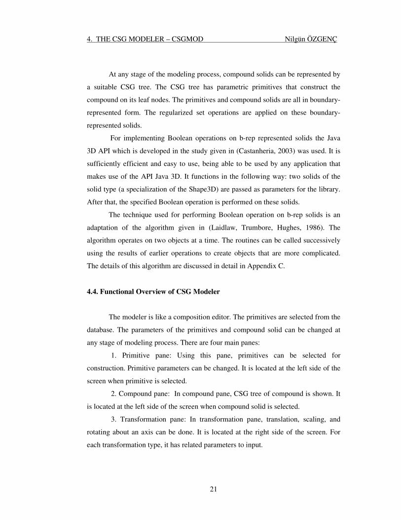
At any stage of the modeling process, compound solids can be represented by

a suitable CSG tree. The CSG tree has parametric primitives that construct the

compound on its leaf nodes. The primitives and compound solids are all in boundary-

represented form. The regularized set operations are applied on these boundary-

represented solids.

For implementing Boolean operations on b-rep represented solids the Java

3D API which is developed in the study given in (Castanheria, 2003) was used. It is

sufficiently efficient and easy to use, being able to be used by any application that

makes use of the API Java 3D. It functions in the following way: two solids of the

solid type (a specialization of the Shape3D) are passed as parameters for the library.

After that, the specified Boolean operation is performed on these solids.

The technique used for performing Boolean operation on b-rep solids is an

adaptation of the algorithm given in (Laidlaw, Trumbore, Hughes, 1986). The

algorithm operates on two objects at a time. The routines can be called successively

using the results of earlier operations to create objects that are more complicated.

The details of this algorithm are discussed in detail in Appendix C.

4.4. Functional Overview of CSG Modeler

The modeler is like a composition editor. The primitives are selected from the

database. The parameters of the primitives and compound solid can be changed at

any stage of modeling process. There are four main panes:

1. Primitive pane: Using this pane, primitives can be selected for

construction. Primitive parameters can be changed. It is located at the left side of the

screen when primitive is selected.

2. Compound pane: In compound pane, CSG tree of compound is shown. It

is located at the left side of the screen when compound solid is selected.

3. Transformation pane: In transformation pane, translation, scaling, and

rotating about an axis can be done. It is located at the right side of the screen. For

each transformation type, it has related parameters to input.


22

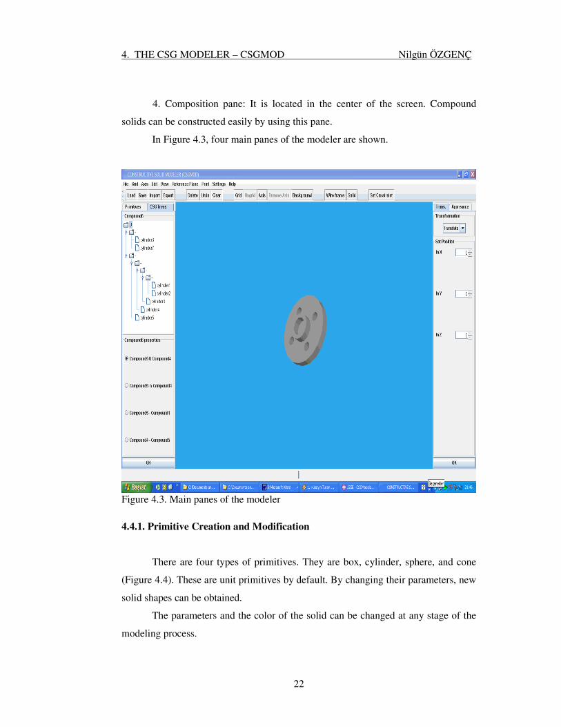
4. Composition pane: It is located in the center of the screen. Compound

solids can be constructed easily by using this pane.

In Figure 4.3, four main panes of the modeler are shown.

Figure 4.3. Main panes of the modeler

4.4.1. Primitive Creation and Modification

There are four types of primitives. They are box, cylinder, sphere, and cone

(Figure 4.4). These are unit primitives by default. By changing their parameters, new

solid shapes can be obtained.

The parameters and the color of the solid can be changed at any stage of the

modeling process.


23

Figure 4.4. Basic primitives: box, sphere, cone, and cylinder

4.4.2. Compound Construction and Modification

A compound solid is constructed from two solids (either primitive or

previously constructed solid) by applying the selected regularized Boolean set

operation on them. Each compound solid has its own CSG tree showing the solids

that construct it and the regularized Boolean set operation applied on it. In Figure

4.5, the construction process of the model is shown. The CSG tree of the selected

compound is on the left pane. The compound can be modified by modifying its

primitives. In addition, the compound can be decomposed into its constructors.


24

Figure 4.5. The construction process of a sample model

4.4.3. Compound Decomposition

Compounds can be decomposed into its constructor solids using the undo

function. Undo function takes the previous regularized Boolean set operation back.

This process is helpful to disassemble the components into its compounds.

4.4.4. Constraint Management

Constraints are used to simply the design process. They define geometrical

relations of each solid with respect to referent. In Figure 4.6, a surface contact

operation is shown. In the modeler, each constraint is defined in vertex, edge, or

surface basis. An offset that is in x, y, and z coordinates can be defined together with

constraint operation.


25

To implement a contact constraint on two solids, the contact referent of each

solids are selecting by pointing the mouse. If it is a vertex contact operation, firstly

the closest vertex of the each solid is found by determining the mouse position. The

distance of these points is calculated in 3D space. Then each point of second solid is

translated by using the distance vector.

Figure 4.6. Surface contact operation

When an edge contact is selected, first the closest edges of each solid are

determined with respect to picking point. Then using these points, true edges of each

solid are determined. After determining the contacting edges, the closest vertices of

each solid are contacted using vertex contact algorithm. Then the angle between


26

these edges is found. Using this angle the rotation matrix to coincide these two edges

on 3D space are calculated. By rotating secondly selected solid using the calculated

matrix, these two edges are coincided.

When a surface contact is requested, first the picked faces of each two solid

are determined. Then the angle between the panes of these surfaces is calculated. By

rotating second solid using this rotation matrix the selected faces of these solids are

coincided.

4.4.5. Applying Transformations

The linear transformations; translation, scaling, and rotation about an axis can

be applied both on compound solids and on primitive solids. The transformations can

be done either using mouse interaction or using transformation pane. Selecting the

solid and by pressing left button of the mouse the solid is translated in X and Y

directions. Selecting the solid and by pressing the right button of the mouse the solid

is rotated in X and Y directions. Selecting the solid and by pressing the mouse

together with alt key the solid is translated in Z direction.

Using the translate option of transformation pane; the selected solid can be

translated in X, Y and Z directions. Using scale option the selected solid is scaled in

X, Y and Z directions. Using rotate option the selected solid is rotated about X, Y,

and Z-axes. Transformation done through the transformation pane is more accurate

than the mouse transformation. For example, using the mouse we cannot put two

parts at 37.5-degree angles.

4.4.6. Copying Primitives and Compounds

The primitives and compound solids can be copied at any stage of modeling

process. Figure 4.7 illustrates copying of some components of the final model. These

newly created compounds again can be used in modeling process.


27

Figure 4.7. Copy operation

4.4.7 Loading and Saving Solid Models

The composed solid can be saved and then can be loaded to modify the solid

or to use the solid in another modeling process. In Figure 4.8, the saving process of

the model is shown. In Figure 4.9, the loading process of the previously saved solid

is shown. The internal save/load format of the modeler includes the java object

definitions of the compound solids and their primitives.


28

Figure 4.8. Save operation

Figure 4.9. Load operation


29

4.5.8. Exporting Graphic Data to Other Formats

Two common formats of interchange graphical data can be exported. The first

one is the industry standard rapid prototyping data format known as STL. The STL

format data of composed solid can be created using the modeler and this data can be

used by rapid prototyping packages.

The other format is widely used OBJ format. The OBJ format data of the

composed solid is exported and the data can be used in almost all 3D modeling

packages.

The modeler can also export the model data in a new generalized format. This

format includes the CSG tree information (how it is composed from primitives) of

composed solid and half-space representations of its primitives. This form of data

can be used for academic studies for simulating CSG algorithms and it can be used

by other packages that support CSG. The CSG graphical data interchange format is

explained in Chapter 5 in detail.

5. THE CSG GRAPHICAL DATA INTERCHANGE FORMAT Nilgün ÖZGENÇ

30

5. THE CSG GRAPHICAL DATA INTERCHANGE FORMAT

5.1. Overview

In CSG, solids are described as combinations of simple primitives or other

solids in a series of Boolean operations. A user operates only on parameterized

instances of solid primitives and Boolean operations on them. Each primitive is

defined either as a combination of half-spaces or triangular mesh.

There is not a generalized format for exporting CSG data together with half-

space primitives. In this study a generalized and simple format for the solid models

that are represented as CSG has been developed. The format is based on the infix

representation of the CSG tree and the half-space representation of each primitive.

We need such a generalized interchange format for the studies related with improved

CSG algorithms studied at the university. Since the modeler is a hybrid modeler, that

boundary representation for primitive representation CSG data for primitives can

also be exported in boundary form (triangular mesh format).

Primitive data can be in three forms. Two of them related with data exchange

between modelers that use CSG model based on half-space data, and one for the

modelers that support CSG on boundary representations:

1. Half-space data including plane equations of each surface that construct the

solid and surface visibility data together with color information. This data can be

used in modelers that use CSG as base representation of the solid.

2. Boundary representation data (triangular meshes that construct the solid):

This data can be used in a dual modeler that based on boundary-represented

primitives.

3. Half-space data including plane depth data together with visibility and color

data: This data is more specific than the first one. This data can be used again in a

CSG based modeler. In addition, it can be used in simulation studies for pixel based

CSG algorithms. The exported data in this form can be used in the simulation of the

algorithm explained in (Koç, 1999)


31

Each of these tree formats has common base files that identify the solid. The

base file includes the number of the primitives, the name of the data file of the

primitives, and the Boolean expression that compose the solid. The name of the

primitive data file is the same names used in the Boolean expression to identify the

primitive.

5.2. Boolean Expression Derivation

Boolean expression of the model is derived from the CSG tree structure of the

modeler. In the expression union is denoted as “+”, intersection is denoted as “.”,

complement is denoted as “!”. Difference is implemented as intersection of first

operand with the complement of second operand. It is denoted as “.!”.

5.3. Plane Equations Derivation

In the modeler, primitives are in triangular mesh format. The vertices are in

counter-clockwise order. Each vertex holds x, y and z values in Cartesian coordinate

system. In the CSG modeler, plane equations can be defined using the vertices of

triangular meshes. The plane equation is

AX + BY + CZ + D = 0 (7.1)

where (A, B, C) is outward face normal of the plane and |D| is the perpendicular

distance of the plane from the origin. Given vertices V1, V2, V3 in counter-

clockwise order: the normal vector of the plane is

N= (V2 – V1) X (V3 – V1) = (A, B, C) (7.2)

where, X denotes a cross product. The value of D is simply the dot product of the

surface normal with any point in the polygon.


32

D=-(N.P) (7.3)

The planes having same equations are eliminated. After this process, the plane

equation of each face that constructs the solid primitive is obtained. The color value

of each face is the color value of the one of the vertexes of it.

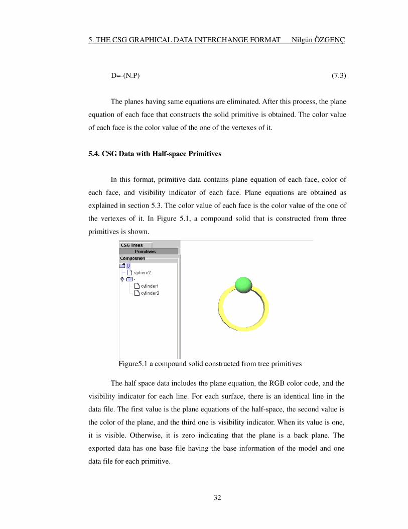
5.4. CSG Data with Half-space Primitives

In this format, primitive data contains plane equation of each face, color of

each face, and visibility indicator of each face. Plane equations are obtained as

explained in section 5.3. The color value of each face is the color value of the one of

the vertexes of it. In Figure 5.1, a compound solid that is constructed from three

primitives is shown.

Figure5.1 a compound solid constructed from tree primitives

The half space data includes the plane equation, the RGB color code, and the

visibility indicator for each line. For each surface, there is an identical line in the

data file. The first value is the plane equations of the half-space, the second value is

the color of the plane, and the third one is visibility indicator. When its value is one,

it is visible. Otherwise, it is zero indicating that the plane is a back plane. The

exported data has one base file having the base information of the model and one

data file for each primitive.


33

5.5. CSG Data with Boundary Represented Primitives

For dual modelers; using boundary representations for presentation and

constructive solid geometry for implementation of the model; primitives are

exported in the polygonal (triangular) mesh format. The Boolean expression format

is the same. This time the data of each primitive is in triangular mesh format. This

data can easily be imported and processed from dual modelers having boundary

representation as the base representation.

5.6. CSG Data with Depth Values

Algorithms, given in (Çevik, 2004), to display a CSG object are based on the

comparisons of distances depth between the viewpoint and surfaces in the scene. The

display space can be considered as a box.

It was shown that the depth value Z, for a plane, whose equation is

AX + BY + CZ + D = 0, can be written as;

Z = (AX + BY + D) / -C (6.4)

where A, B, C, and D are the plane coefficients in the display space and X and Y are

the coordinates of pixel position on the screen. If C=0, that occurs each time a plane

is perpendicular to the screen, another value K can be defined. K is the perpendicular

distance between the pixel and the plane.

K = AX + BY + D (6.5)

These equations can be written as:

Z(x, y) = Zo + XdZx + YdZy (6.6)


34

K(x, y) = Ko + XdKx + YdKy (6.7)

where, Zo and Ko are the Z and K values at the origin while dZx, dZy, dKx, dKy are

differential increments of Z and K along X and Y-axes.

dZx = dZ/dX = A/(-C) (6.8)

dZy = dZ/dY = B/(-C) (6.9)

dKx = A (6.10)

dKy = B (6.11)

Together with these values, some other values required for displaying

algorithms. These are the perpendicularity of the plane to the screen, visibility of the

surface (whether it is back or front surface) and the convexity of the surface (whether

it is convex or concave). In our case, the surfaces are always convex. The plane is

perpendicular to the screen if its value of the C coefficient is zero. The plane is

visible from a viewpoint is a front face and those invisible from the viewpoint is back

surface.

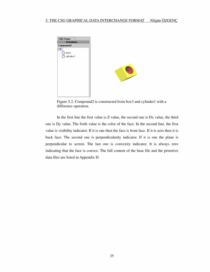
In Figure 5.2, a compound that is constructed from two primitives is shown.

The Boolean expression exported for this model is “box3.!cylinder1”.

The CSG data file for the primitives have two lines of information for each

face. In first line the depth values and the color of the face is defined. In second line,

indicators are defined. The first for line of the data file of box3 is as follows:

207.66 -1.06 -0.39 0

1 0 0

368.15 -1.06 -0.39 0

0 0 0


35

Figure 5.2. Compound2 is constructed from box3 and cylinder1 with a difference operation.

In the first line the first value is Z value, the second one is Dx value, the third

one is Dy value. The forth value is the color of the face. In the second line, the first

value is visibility indicator. If it is one then the face is front face. If it is zero then it is

back face. The second one is perpendicularity indicator. If it is one the plane is

perpendicular to screen. The last one is convexity indicator. It is always zero

indicating that the face is convex. The full content of the base file and the primitive

data files are listed in Appendix D.

6. RESULTS AND DISCUSSIONS Nilgün ÖZGENÇ

36

6. RESULTS AND DISCUSSIONS

STL format data of solid models was tested by using the 3D view and markup

package named as SolidView and another viewing package named as DeskArtes

View. The OBJ format was also tested by using this package. In Figure 6.1, the STL

format SolidView display of a model constructed using the CSGMOD is shown. In

Figure 6.2, the OBJ format DeskArtes View display of a model that is exported from

the modeler tool is shown.

Figure 6.1. The display of the STL formatted model on the SolidView package

The modeling tool is developed in Java. The main advantages of Java are its

compatibility across different systems/platforms and having the ability to be run

remotely through web browsers. Using Java 3D as a graphics engine has also the

additional advantage of rapid application development, because Java 3D API

incorporates a high-level scene graph model that allows developers to focus on the


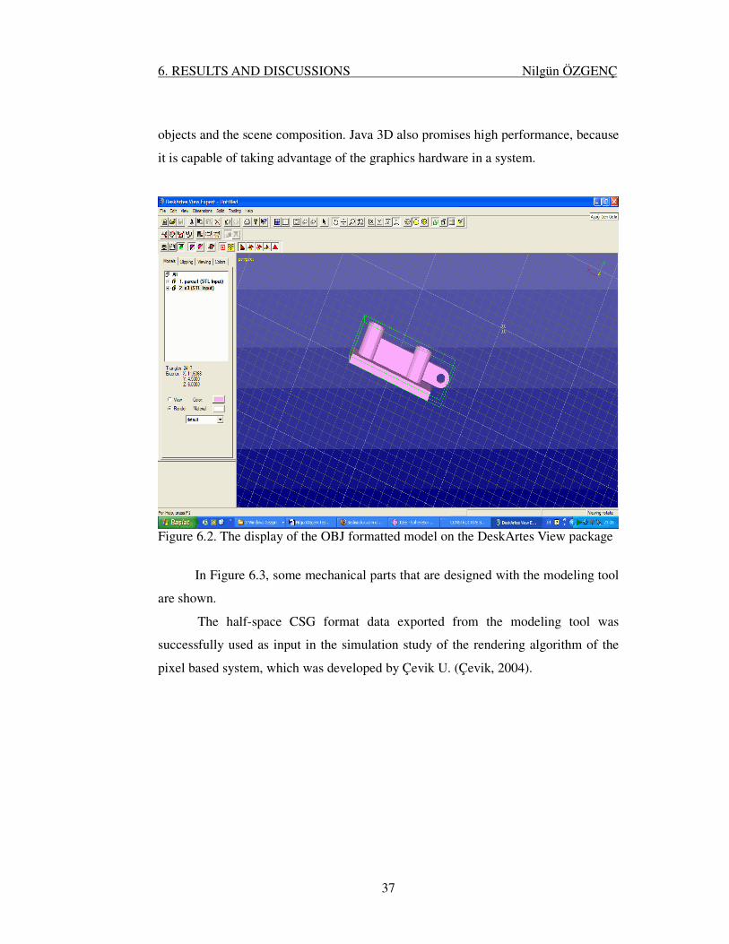
37

objects and the scene composition. Java 3D also promises high performance, because

it is capable of taking advantage of the graphics hardware in a system.

Figure 6.2. The display of the OBJ formatted model on the DeskArtes View package

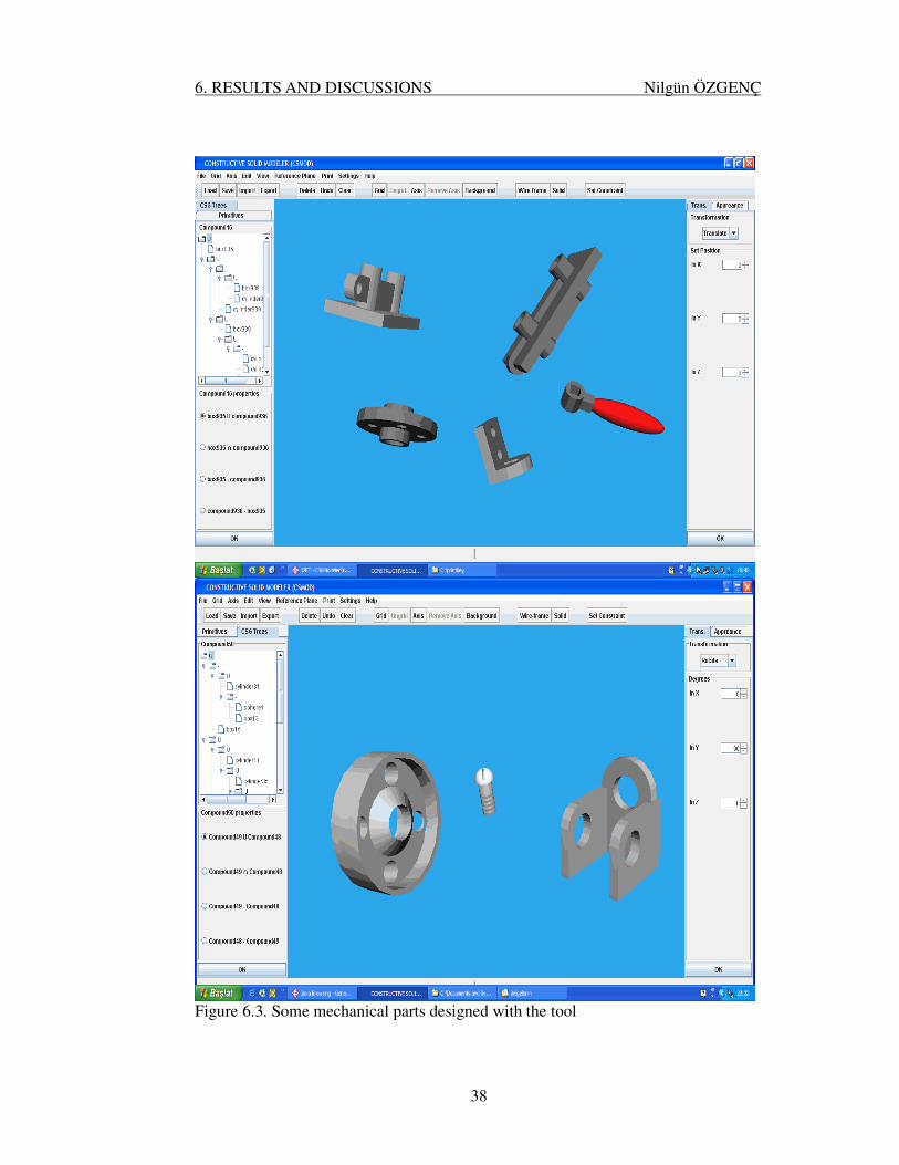
In Figure 6.3, some mechanical parts that are designed with the modeling tool

are shown.

The half-space CSG format data exported from the modeling tool was

successfully used as input in the simulation study of the rendering algorithm of the

pixel based system, which was developed by Çevik U. (Çevik, 2004).


38

Figure 6.3. Some mechanical parts designed with the tool

7.CONCLUSIONS AND FUTURE WORK Nilgün ÖZGENÇ

39

7. CONCLUSIONS AND FUTURE WORK

In this study an interactive solid modeler tool that exports a generalized

graphical data in forms of half-space CSG representation has been developed. The

traditional CSG systems are based on image-space CSG rendering algorithms. The

image-spaced algorithms run on pixel-planes and can be executed in parallel per

pixel basis. Because of this fact, the image-space CSG algorithms are faster.

However, image-space CSG algorithms are not suitable for interactive modeling

process because of the fact that they have no adjacency information. Because of the

fact, the solid modeler uses an object-space CSG algorithm. By having the adjacency

information, the modeling process can be simplified by using geometric constraints.

In addition, during interactive solid modeling, the modeling process has many

processes that are not directly related with the CSG process. When such a process is

performed, the display is rendered using a polygonal renderer. If an image-space

CSG algorithms use instead, the CSG algorithm must be evaluated each time the

display is refreshed even if that this does not requires the CSG implementation of the

model. Since in the modeler tool the adjacency information is required for constraint

processing and the model is interactively created on the scene graph using various

non-CSG related operations, in the tool, the object space CSG algorithm on boundary

representation approach is used.

The CSG modeling tool can export the graphical data of the final model in a

new general format. The format includes the CSG expression that forms the final

model and the graphical data of the each primitive in both polygonal and half-space

format. In addition, the final model’s graphical data is exported in both half-space

and polygonal representation forms. In these formats, the CSG tree structure contains

the hierarchical structure of the model. This implements the part assembly of the

model. This data is very helpful in the reverse engineering of the design process of

solid models.

The half-space represented CSG format of the solid models can be used in

reverse engineering, pixel based rendering algorithms, simulation work of pixel

based GPU algorithms, animation. Since the exported data is in part assembly

7.CONCLUSIONS AND FUTURE WORK Nilgün ÖZGENÇ

40

structure, in animation different motions can be defined for each part of the model. In

addition, the related motions can also be defined with more than two parts.

In image-based rendering GPUs depth valued half-space data can be used for

simulation purposes.

Planned future work includes speeding up and simplifying the modeling

process. Modeling process will be speeded up by adding more predefined primitives,

adding predefined features (such as holes, fillets, rounds) and adding more constraint

definitions (angular constraints, reference planes etc.). In addition, the construction

of the CSG tree structures of the imported boundary represented models will be

handled. To construct the CSG tree structure of a boundary model, firstly the model

is imported to the tool and then using the boundary to CSG conversion algorithms,

the CSG tree structure of the boundary model will be obtained. Obtaining the

structural CSG models of the boundary models are useful in reverse engineering for

obtaining the structural design and components of the models.

41

REFERENCES

BUTLER, L. A., EDWARDS, and E. W., KREGEL, D. L., 2003. BRL-CAD Tutorial

Series: Volume III – Principles of Effective Modeling; ARL-SR-119; U.S.

Army Research Laboratory: Aberdeen Proving Ground, MD, 88p.

CASTANHERIA, D.B.S., 2003. Agreed Constructive Solid Geometry of Solids to

The Representation B-rep. Graduation Project, University of Brasilia,

Department of Computer Sciences, 102p.

ÇEVİK, U., 2004. Design and Implementation of an FPGA-based Parallel Graphics

Renderer for CSG Surfaces and Volumes. Computers and Electrical

Engineering 30: p.97-117.

FOLEY, J.D., 1993. Introduction to Computer Graphics, Addison Wesley, 632p.

FOLEY, J.D., VAN, D.A., FEINER S.K., and HUGHES, J.F., 1996. Computer

Graphics: Principles and Practice. Second Edition, Addition-Wesley, 1200p.

JAVA 3D API. 2006. java.sun.com/products/java-media/3D/

KOC, S., 1999. Development of an Algorithm For the Elimination of Surface Sorting

in the Stage of Removal in Displaying Constructive Solid Geometry Volumes

and Surfaces. University of Gaziantep M.Sc. Thesis, p.1-122.

LAIDLAW, D.H., TRUMBORE W.B., HUGHES J.F. 1986. Constructive solid

Geometry for polyhedral objects. ACM International Conference on

Computer Graphics and Interactive Techniques: p.161-170.

MACMAINS, S.A., 2000. Geometric Algorithms and Data Representation for Fee

For Fabrication. Dphil. Thesis, University of California, Berkeley, 171p.

MANTYLA, M., 1988. An Introduction to Solid Modeling. Computer Science Press.

SHAPIRO, V., 2001. Solid Modeling. Handbook of Computer Aided Geometric

Design, Elsevier Science Publishers, p.473-518.

WOLFE, R., 1998. 3D Freebies: A Guide to High Quality 3D Software Available via

the Internet. ACM SIGGRAPH. Volume: 2. No: 2.

42

APPENDIX A: A SAMPLE STL FILE

Stl file of the cube:

solid box1

FACET NORMAL -0.5597179740814301 0.5543062663151178 -0.6160035329557562 OUTER LOOP vertex -0.7474092974917155 -0.25091999844497953 -0.3583552656279948 vertex -0.6330651618766918 0.5369820176977205 0.2467363238100999 vertex 0.1876913234102855 0.805226264760097 -0.2576482673277597 ENDLOOP ENDFACET FACET NORMAL -0.5597179740814305 0.5543062663151181 -0.6160035329557556 OUTER LOOP vertex 0.1876913234102855 0.805226264760097 -0.2576482673277597 vertex 0.07334718779526138 0.0173242486173971 -0.8627398567658549 vertex -0.7474092974917155 -0.25091999844497953 -0.3583552656279948 ENDLOOP ENDFACET FACET NORMAL 0.5597179740814299 -0.5543062663151179 0.6160035329557563 OUTER LOOP

43

vertex -0.18769132341028538 -0.8052262647600968 0.2576482673277593 vertex 0.6330651618766917 -0.5369820176977205 -0.24673632381009986 vertex 0.7474092974917156 0.2509199984449794 0.35835526562799475 ENDLOOP ENDFACET FACET NORMAL 0.5597179740814303 -0.5543062663151183 0.6160035329557555 OUTER LOOP vertex 0.7474092974917156 0.2509199984449794 0.35835526562799475 vertex -0.07334718779526149 -0.01732424861739703 0.862739856765855 vertex -0.18769132341028538 -0.8052262647600968 0.2576482673277593 ENDLOOP ENDFACET FACET NORMAL -0.11434413561502405 -0.7879020161427004 -0.6050915894380957 OUTER LOOP vertex -0.7474092974917155 -0.25091999844497953 -0.3583552656279948 vertex 0.07334718779526138 0.0173242486173971 -0.8627398567658549 vertex 0.6330651618766917 -0.5369820176977205 -0.24673632381009986 ENDLOOP ENDFACET FACET NORMAL -0.11434413561502396 -0.7879020161427001 -0.605091589438096 OUTER LOOP vertex 0.6330651618766917 -0.5369820176977205 -0.24673632381009986 vertex -0.18769132341028538 -0.8052262647600968 0.2576482673277593 vertex -0.7474092974917155 -0.25091999844497953 -0.3583552656279948 ENDLOOP ENDFACET FACET NORMAL 0.8207564852869771 0.2682442470623769 -0.5043845911378607 OUTER LOOP vertex 0.07334718779526138 0.0173242486173971 -0.8627398567658549 vertex 0.1876913234102855 0.805226264760097 -0.2576482673277597 vertex 0.7474092974917156 0.2509199984449794 0.35835526562799475 ENDLOOP ENDFACET FACET NORMAL 0.8207564852869772 0.2682442470623767 -0.5043845911378606 OUTER LOOP vertex 0.7474092974917156 0.2509199984449794 0.35835526562799475 vertex 0.6330651618766917 -0.5369820176977205 -0.24673632381009986 vertex 0.07334718779526138 0.0173242486173971 -0.8627398567658549 ENDLOOP ENDFACET

44

FACET NORMAL 0.11434413561502384 0.7879020161427005 0.6050915894380957 OUTER LOOP vertex 0.1876913234102855 0.805226264760097 -0.2576482673277597 vertex -0.6330651618766918 0.5369820176977205 0.2467363238100999 vertex -0.07334718779526149 -0.01732424861739703 0.862739856765855 ENDLOOP ENDFACET FACET NORMAL 0.11434413561502439 0.7879020161427003 0.6050915894380958 OUTER LOOP vertex -0.07334718779526149 -0.01732424861739703 0.862739856765855 vertex 0.7474092974917156 0.2509199984449794 0.35835526562799475 vertex 0.1876913234102855 0.805226264760097 -0.2576482673277597 ENDLOOP ENDFACET FACET NORMAL -0.8207564852869769 -0.26824424706237704 0.5043845911378606 OUTER LOOP vertex -0.6330651618766918 0.5369820176977205 0.2467363238100999 vertex -0.7474092974917155 -0.25091999844497953 -0.3583552656279948 vertex -0.18769132341028538 -0.8052262647600968 0.2576482673277593 ENDLOOP ENDFACET FACET NORMAL -0.8207564852869772 -0.2682442470623771 0.5043845911378602 OUTER LOOP vertex -0.18769132341028538 -0.8052262647600968 0.2576482673277593 vertex -0.07334718779526149 -0.01732424861739703 0.862739856765855 vertex -0.6330651618766918 0.5369820176977205 0.2467363238100999 ENDLOOP ENDFACET endsolid

45

APPENDIX B: A SAMPLE OBJ FILE (from WAVEFRONT)

Cube with Materials

# This cube has a different material # applied to each of its faces. mtllib master.mtl v 0.000000 2.000000 2.000000 v 0.000000 0.000000 2.000000 v 2.000000 0.000000 2.000000 v 2.000000 2.000000 2.000000 v 0.000000 2.000000 0.000000 v 0.000000 0.000000 0.000000 v 2.000000 0.000000 0.000000 v 2.000000 2.000000 0.000000 # 8 vertices g front usemtl red f 1 2 3 4 g back usemtl blue f 8 7 6 5 g right usemtl green f 4 3 7 8 g top usemtl gold f 5 1 4 8 g left usemtl orange f 5 6 2 1 g bottom usemtl purple f 2 6 7 3 # 6 elements

Bezier Patch

# 3.0 Bezier patch v -5.000000 -5.000000 0.000000 v -5.000000 -1.666667 0.000000 v -5.000000 1.666667 0.000000 v -5.000000 5.000000 0.000000 v -1.666667 -5.000000 0.000000 v -1.666667 -1.666667 0.000000 v -1.666667 1.666667 0.000000 v -1.666667 5.000000 0.000000

46

v 1.666667 -5.000000 0.000000 v 1.666667 -1.666667 0.000000 v 1.666667 1.666667 0.000000 v 1.666667 5.000000 0.000000 v 5.000000 -5.000000 0.000000 v 5.000000 -1.666667 0.000000 v 5.000000 1.666667 0.000000 v 5.000000 5.000000 0.000000 # 16 vertices cstype bezier deg 3 3 # Example of line continuation surf 0.000000 1.000000 0.000000 1.000000 13 14 \ 15 16 9 10 11 12 5 6 7 8 1 2 3 4 parm u 0.000000 1.000000 parm v 0.000000 1.000000 end # 1 element

Cardinal Curve

# 3.0 Cardinal curve v 0.940000 1.340000 0.000000 v -0.670000 0.820000 0.000000 v -0.770000 -0.940000 0.000000 v 1.030000 -1.350000 0.000000 v 3.070000 -1.310000 0.000000 # 6 vertices cstype cardinal deg 3 curv 0.000000 3.000000 1 2 3 4 5 6 parm u 0.000000 1.000000 2.000000 3.000000 end # 1 element

Texture-Mapped Square

# A 2 x 2 square mapped with a 1 x 1 square # texture stretched to fit the square exactly. mtllib master.mtl v 0.000000 2.000000 0.000000 v 0.000000 0.000000 0.000000 v 2.000000 0.000000 0.000000 v 2.000000 2.000000 0.000000 vt 0.000000 1.000000 0.000000 vt 0.000000 0.000000 0.000000 vt 1.000000 0.000000 0.000000 vt 1.000000 1.000000 0.000000 # 4 vertices

47

usemtl wood # The first number is the point, # then the slash, # and the second is the texture point f 1/1 2/2 3/3 4/4 # 1 element

48

APPENDIX C: THE OBJECT-SPACE CSG ALGORITM

The object-space CSG algorithm used in this study is an adaptation of the

algorithm given in (Laidlaw, Trumbore, Hughes, 1986). This adaptation is

implemented as a Java3D API by Castanheria, D.B.S. (Castanheria, 2003). This

Java3D API is used in the study for implementing Boolean operations on b-rep

represented solids which surfaces are defined in triangulated polygons form.

In the algorithm, there are five restrictions related with polygons:

1. It must be planar and convex.

2. No three vertices in the polygon may be collinear.

3. It may not contain the same vertex twice.

4. The vertices must be ordered clockwise when viewed from outside the

object, so that cross products using the directed edges of the polygon may be used to

determine the interior of the object.

5. No polygon may intersect any other polygon in the object.

Since the triangulated polygons are used in the implementation, all these

restrictions are satisfied.

The structures used in algorithms are object, vertex, and polygon structure.

The object data structure includes array of vertices, array of polygons and object

extent. The vertex structure contains its spatial location, array of pointers to adjacent

vertices, and its status (inside, outside, boundary, or unknown). The polygon

structure includes array of pointers to vertices, polygon extent and polygon plane

equation. There are tree main steps of the algorithm:

1. Subdivide all polygons in each of the operand object so that no two

polygons intersect.

49

2. Classify the polygons of each object with respect to surface of the other

object. A polygon in one object may lie inside, outside, or on the boundary of the

other object.

3. Use the classification of polygon to retain or delete it according to the set

operation being performed.

At the beginning, status values of all vertices are set as UNKNOWN. The

main steps of the surface dividing algorithm are:

. split first object so that it does not intersect the second object

. split second object so that it does not intersect the first object

. split the first object again to resolve intersection caused by the above

steps

By naming the two objects as objectA and objectB, the algorithm of splitting

objectA by objectB is as fallows:

if extent of one objectA overlaps the extent of the objectB

for each polygonA in objectA

if the extent of polygonA overlaps the extent of objectB

for each polygonB in objectB

if extents of polygonA and polygonB overlap

analyze them by using Polygon Intersection Check Algorithm

if they are not COPLANAR and do not INTERSECT

subdivide polygonA as in Subdividing Non-Coplanar

Polygons Algorithm

else if they do not intersect

or they are COPLANAR do nothing

Extent values are set the maximum and minimum x, y, and z values of the

each polygon or each object respectively.

50

Polygon intersection check algorithm is use to determine whether two

polygons are coplanar, intersect in a line or a point, or do not intersect. In this

algorithm, the main idea is finding the intersection position status of polygonA with

respect to polygonB.

find the signed distance from each of vertices in polygonA to the plane of

polygonB.

if these distance values are all zero, then the polygons are coplanar.

if they are all positive, or negative then polygonA lies entirely on one side of

the polygonB meaning that these two polygons do not intersect.

otherwise they may intersect

In case of otherwise of the above algorithm, another method is used. The line

of intersection of two planes is calculated. This line L is determined by a point P and

its direction vector D. P can be any pertaining point to the planes of the two faces,

and D can be calculated by a vector multiplication of the normal ones of the faces. If

the interior and perimeter segments of line with respect to polygonA overlap those of

PolygonB, then the polygons intersect.

After finding the intersecting polygons, a segment data structure is defined.

This data structure includes the distance from P to the starting end ending points of

the segment, and will be used later in the subdividing non-planar polygons algorithm.

The segment data structure is filled according to the way that the line L intersects the

polygons. The six possibilities of intersection of a polygon and a line in a plane are

shown is figure C.1.

51

Figure C.1. Intersection possibilities of a polygon and a line in a plane (a) vertex-vertex-vertex (b) vertex-edge-vertex (c) vertex-face-vertex (d) vertex-face-edge (e) edge-face-edge (Laidlaw, Trumbore, Hughes, 1986)

The subdividing non-coplanar polygons algorithm is used to subdivide non-

coplanar polygons so that the resulting polygons do not intersect. It based on the

intersection segment status of one object with respect to the other’s intersection

segment.

In the polygon-classifying algorithm, the average of the vertices of a polygon

is called barycenter. The polygon classification routine is as fallows (taken from the

study explained in (Laidlaw, Trumbore, Hughes, 1986)):

create a RAY starting at the barycenter of polygonA in the direction of the normal of polygonA while no successful cast has been made for each polygonB in objectB find the DOT PRODUCT of RAY direction with the normal of polygonB find the DISTANCE from barycenter to the plane of polygonB if (DOT PRODUCT = 0) and (DISTANCE = 0) cast is unsuccessful -- leave loop and perturb else if (DOT PRODUCT = 0) and (DISTANCE > 0) no intersection else if (DOT PRODUCT <> 0) and (DISTANCE = 0) if RAY passes through interior or edge of polygonB save polygonB -- this is closest possible intersection else no intersection else if (DOT PRODUCT <> 0) and (DISTANCE > 0) find intersection point of ray with plane of polygonB

52

if intersection is closest yet if RAY passes through interior of polygonB (first, check if point is within extent of polygonB) save polygonB else if RAY hits an edge of polygonB cast is unsuccessful - leave loop and perturb else no intersection if cast is unsuccessful perturb RAY by a small random value end while if there were no intersections return OUTSIDE find the polygonB closest to POINT find the DOT PRODUCT of closest polygonal normal and RAY find the DISTANCE to closest polygonB if (DISTANCE == 0) if (DOT PRODUCT > 0) return SAME else if (DOT PRODUCT < 0) return OPPOSITE else if (DOT PRODUCT > 0) return INSIDE else if (DOT PRODUCT < 0) return OUTSIDE

To classify the vertices still marked as UNKNOWN first region marking

routine is used to calculate the adjacency information for each object. Then vertex

marking routine is used to classify the vertices still having UNKNOWN values.

These routines are as fallows (taken from the study explained in (Laidlaw, Trumbore,

Hughes, 1986)):

Region-Marking Routine:

calculate adjacency information for all vertices of objectA

for each polygonA in objectA

if any vertices are marked UNKNOWN

call Polygon Classification Routine

to determine if polygonA INSIDE/OUTSIDE objectB

for each UNKNOWN vertex in polygonA

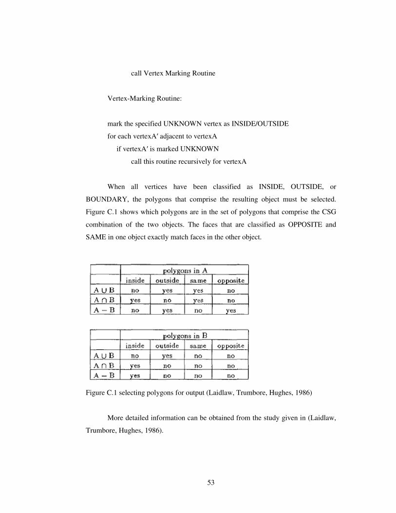
53

call Vertex Marking Routine

Vertex-Marking Routine:

mark the specified UNKNOWN vertex as INSIDE/OUTSIDE

for each vertexA′ adjacent to vertexA

if vertexA′ is marked UNKNOWN

call this routine recursively for vertexA

When all vertices have been classified as INSIDE, OUTSIDE, or

BOUNDARY, the polygons that comprise the resulting object must be selected.

Figure C.1 shows which polygons are in the set of polygons that comprise the CSG

combination of the two objects. The faces that are classified as OPPOSITE and

SAME in one object exactly match faces in the other object.

Figure C.1 selecting polygons for output (Laidlaw, Trumbore, Hughes, 1986)

More detailed information can be obtained from the study given in (Laidlaw,

Trumbore, Hughes, 1986).

54

APPENDIX D: CSG DATA WITH DEPTH VALUES

The base file

2 box3.pln cylinder1.pln box3.!cylinder1 The data file for box3

207.66 -1.06 -0.39 0 1 0 0 368.15 -1.06 -0.39 0 0 0 0 19.77 0.75 0.53 0 0 0 0 679.12 3.44 -6.7 0 1 0 0 -124.84 0.75 0.53 0 1 0 0 1488.4 3.44 -6.7 0 0 0 0

The data file for cylinder1

272.6 -0.67 -0.63 1 1 0 0 34.18 1.54 -0.05 1 0 0 0 -19.4 1.09 0.42 1 0 0 0 -56.28 0.73 0.81 1 0 0 0 -88.05 0.35 1.21 1 0 0 0 -123.18 -0.17 1.76 1 0 0 0 -181.4 -1.24 2.89 1 0 0 0 -497.82 -8.03 10.1 1 0 0 0 82.99 5.01 -3.74 1 1 0 0 -48.33 2.32 -0.88 1 1 0 0 -94.09 1.54 -0.05 1 1 0 0

55

-126.9 1.09 0.42 1 1 0 0 -159.52 0.73 0.81 1 1 0 0 -200.39 0.35 1.21 1 1 0 0 -265.16 -0.17 1.76 1 1 0 0 -412.03 -1.24 2.89 1 1 0 0 -1402.55 -8.03 10.1 1 1 0 0 525.88 5.01 -3.74 1 0 0 0 138.58 2.32 -0.88 1 0 0 0 417.58 -0.67 -0.63 1 0 0 0

56

APPENDIX E: THE HIERARCHICAL STRUCTURE OF A SOLID MODEL

The hierarchic structure of a solid model implemented in the tool is shown in

Figure E.1.

Figure E.1 Hierarchic structure of a solid model in the tool

Shape3D is the class of Java 3D that is used to represent Java3D object on the

SceneGraph. The class hierarchy of the Shape3D is as follows.

″The Shape3D leaf node specifies all geometric objects. It contains a list of

one or more Geometry component objects and a single Appearance component

object. The geometry objects define the shape node's geometric data. The appearance

object specifies that object's appearance attributes, including color, material, texture,

and so on.

The list of geometry objects must all be of the same equivalence class, that is,

the same basic type of primitive. For subclasses of GeometryArray, all point objects

are equivalent, all line objects are equivalent, and all polygon objects are equivalent.

For other subclasses of Geometry, only objects of the same subclass are equivalent.

The equivalence classes are as follows:

57

• GeometryArray (point): [Indexed]PointArray

• GeometryArray (line): [Indexed]{LineArray, LineStripArray}

• GeometryArray (polygon): [Indexed]{TriangleArray,

TriangleStripArray, TriangleFanArray, QuadArray}

• CompressedGeometry

• Raster

• Text3D

When Shape3D is used with multiple geometry components, Java 3D may

choose to use individual geometry bounds instead of the shape's bounds for region of

influence operations, such as lighting. For example, the individual characters of a

Text3D shape object may be rendered with a different light set.″ (JAVA3D API,

2006).

The Solid structure is used handle the boundary representation of the solid

model. The vertices, edges, surface data, and their adjacency information are stored

in this structure.

The CSGSolid structure is used for handling the CSG tree description of the

objects. It also has a total transformation matrix for each solid that holds the total

transformation done to the solid during the modeling process.

The CompoundSolid structure has the following data: the operand solids of

the compound solid that construct it and the Boolean set operation applied.

The PrimitiveSolid class is used to handle primitive data. Each primitive can be box,

cylinder, cone, or sphere.

The box primitive is defined by its three parameters: width, height, and

length. The box is defined as a twelve triangulated surface having the vertices of

these triangles and the information how this vertices are connected.

The cylinder primitive is defined by its height and the ray value of x and z. It

defined with 20 surfaces; two for bottom and up, and 18 for cylindrical half body. In

internal representation, it is represented as a connection of 216 triangles.

58

The sphere primitive is defined by its ray values along the x, y, and z-axis. In

internal representation, it is represented as 960 triangles, which are connected

through 482 edges.

The cone primitive is defined by its height and the ray value of x and z. It is

internally defined as a connected set of 288 triangles.

In all primitives, the center and some specific coordinates (such as top point

of cone) are also stored in related primitive structures. These coordinates are used in

constraint definitions.

59

BIOGRAPHY

Nilgün Özgenç received the B.S. degree in Computer Engineering from

Middle East Technical University, Ankara, Turkey, in 1987. After completion her

B.S. training, she worked in IT sector for 17 years. She experienced in system

programming of IBM mainframe (VSE, VM, MVS, OS/390), IBM middle-sized

systems (S/36, S/38, OS/400, and IBM UNIX (AIX)), and small-sized computers

(Microsoft Windows, and Linux). She worked at several IT projects such as;

installation and configuration of operating systems and their subsystems,

maintenance and management of operating systems and their subsystems,

performance tuning, security management of IT systems, operations improvements

for IT departments, disaster recovery planning, synchronous and asynchronous

communication of applications, program-to-program communication, network

performance management, network traffic management, reengineering of IT

processes, client/server application development methodologies, database design and

management for application packages and decision support systems, change and

version management systems, problem management systems, atomization of system

maintenance and management processes, installation, maintenance, and management

of the application based software packages such as SAP, Millennium, AMAPS-Q

and so on.

She has started MSc degree in the department of Electrical and Electronics

Engineering in Çukurova University at September 2004. She has been working in

Çukurova University as a specialist since September 2005.

Her areas of interest include computer graphics, database management

systems, SAP basis consultancy, system engineering on IBM systems, on UNIX

systems, and on Microsoft Windows and Linux systems, system analysis, and design

of application packages, reengineering of IT departments, disaster recovery planning,

and security management of IT systems.

60

LIST OF PUBLICATIONS

[1] SCIENTIFIC COLLABORATION FOR SUSTAINABLE DEVELOPMENT

2007, TURKEY

An Interactive Constructive Solid Geometry Modeling Tool

Çevik ULUS Nilgün ÖZGENÇ

Department of Electrical & Electronics Engineering, Çukurova University, Adana, Turkey

Abstract: In Constructive Solid Geometry (abbreviated CSG) modeling, creating solid models interactively will speed up the modeling process. In this work, a software tool for creating CSG solid models is given. By means of this tool, modeling will be interactive and so, the designer will work with more efficiency and less time. The CSG models are very suitable for holding hierarchical structure of the solid models. This work is motivated by the need of obtaining the half space CSG representation of a solid model interactively. The CSG tree description and the half space representation of the solid model can provide useful information in the area of reverse engineering and in other areas relating with solid modeling as well.

Index Terms: Constructive solid geometry, pixel processor, half-spaces, solid modeler

university of Çukurova institute of …library.cu.edu.tr/tezler/6415.pdf · i would like to thank...

Documents