university of arizona-full text...
TRANSCRIPT

Modeling Stream-Aquifer Interactions During Floods andBaseflow: Upper San Pedro River, Southeastern Arizona
Item Type text; Electronic Thesis
Authors Simpson, Scott
Publisher The University of Arizona.
Rights Copyright © is held by the author. Digital access to this materialis made possible by the University Libraries, University of Arizona.Further transmission, reproduction or presentation (such aspublic display or performance) of protected items is prohibitedexcept with permission of the author.
Download date 07/06/2018 09:22:41
Link to Item http://hdl.handle.net/10150/193338

MODELING STREAM-AQUIFER INTERACTIONS DURING FLOODS AND
BASEFLOW: UPPER SAN PEDRO RIVER, SOUTHEASTERN ARIZONA.
by
Scott Carlyle Simpson
__________________________________ Copyright © Scott Carlyle Simpson 2007
A Thesis Submitted to the Faculty of the
DEPARTMENT OF HYDROLOGY AND WATER RESOURCES
In Partial Fulfillment of the Requirements
For the Degree of
MASTER OF SCIENCE WITH A MAJOR IN HYDROLOGY
In the Graduate College
THE UNIVERSITY OF ARIZONA
2007

2
STATEMENT BY AUTHOR This thesis has been submitted in partial fulfillment of requirements for an advanced degree at The University of Arizona and is deposited in the University Library to be made available to borrowers under rules of the Library.
Brief quotations from this thesis are allowable without special permission, provided that accurate acknowledgement of source is made. Requests for permission for extended quotation from or reproduction of this manuscript in whole or in part may be granted by the copyright holder.
SIGNED: ________Scott C. Simpson_________
APPROVAL BY THESIS DIRECTOR This thesis has been approved on the date shown below:
______________________________ November 5, 2007 . Thomas Meixner Date Professor of Hydrology

3
ACKNOWLEDGEMENTS
I would like to thank the following people (in no particular order) for their help at various points during the duration of this research project: Thomas Meixner (UA-HWR): Thank you for all the mental time and effort
exerted during this project: both in getting it started and in guiding it in the proper directions between then and completion.
James Leenhouts (USGS-Tucson): Thank you for your initial input and expertise
regarding the study area and for allowing the use of so much of your data in this model. It is safe to say that this project would not have been possible to the extent that it was without your data.
Bill Childress (BLM): Thank you for allowing access to the study sites in SPRNCA and for dealing personally with the myriad accessibility issues early on. Kate Baird (UA-HWR): Thank you for allowing the use of the ET curves you developed with Drs. Maddock and Stromberg. They proved to be a truly integral component of this model. James Hogan (UA-HWR, SAHRA): Thank you for providing such helpful and constructive criticisms regarding this thesis and for steering this manuscript in the proper direction for the subsequent journal submission. Carlos Soto, Jeff Gawad and Caitlin Zlatos (UA-HWR): Thank your all for your help in the field and/or lab.

4
TABLE OF CONTENTS
ABSTRACT….………… ………………………………………………...………....7
1. INTRODUCTION…... ………………………………………………...………....9
2. STUDY AREA / BACKGROUND…. ..……………………………...………... 12
3. FIELD SAMPLING & ANALYTICAL METHODS..…...…………......……... 14
4. MODEL STRUCTURE: WATER BALANCE …….. .………………...…….....16
4.1 Background.………….…………...…………………………...…….…16
4.2 Model Domain Partitioning....……....……………………………….…17
4.3 Basin/Riparian Groundwater Exchange and Evapotranspiration.…..….18
4.3.1 Gaining River Reach ET and Groundwater Estimates……....…19
4.3.2 Losing River Reach ET and Groundwater Estimates …….....…21
4.4 River/Aquifer Exchange ………………………………………….…....24
4.4.1 Diffusivity Estimation ……….………………………….....…...26
4.5 Transfer of Water Downstream.…......…………………………….…...27
5. MODEL STRUCTURE: CONSERVATIVE TRACERS…... ..……….………..30
5.1 Summary: Tracking Water Movement Through The Model. ..….……..30
5.2 Basin/Riparian Groundwater Exchange……. .……….………………...31
5.3 Evapotranspiration.… …………………………………....……….……32
5.4 River/Aquifer Exchange……..…………………….....………..…….…33
5.5 Transfer of Water Downstream...........…………….…………..…….…34

5
TABLE OF CONTENTS – Continued
6. MODEL INPUTS…… ……………………………………...….…………….....35
6.1 Streamflow Volume.……….. .………………………………..…….….35
6.2 Surface Flow Chemistry…… .………………………………..…….….36
6.3 Groundwater Flux and Chemistry.…. .…………….…………..…….....37
7. MODEL OUTPUTS…………………….……...………….………………….....39
8. RESULTS: BASE-CASE MODEL SIMULATION.......…....…....……………..40
8.1 Water Balance Results.…….. …..………….……….………………….40
8.2 Chemical and Isotopic Results .……. …..….……………….………….43
9. SENSITIVITY ANALYSIS….……... ……………...…….…………………….45
9.1 Methodology & Results.…… ……………...…….…………………….45
9.2 Discussion….. .……………………...…………………………..……...47
9.3 Chemical/Isotopic Sensitivity Analysis……. ……………………..…...49
10. MANUAL CALIBRATION, RESULTS & DISCUSSION.. .……..…...….…..50
10.1 Results & Discussion: Water Balance.…….. ……………….....……....51
10.2 Results & Discussion: Chemical/Isotopic Composition.…... ……..…...53
11. QUANTIFYING STREAM CHANNEL RECHARGE:
OVERALL SUMMARY & CONCLUSIONS…….. ………...…..........60
12. IMPLICATIONS FOR FURTHER RESEARCH … ………...………...……...65

6
TABLE OF CONTENTS – Continued
APPENDICES…………………………...……………………...………………….66
APPENDIX A: FIGURES……………………………...………………………67
APPENDIX B: TABLES …………………………….………....…………….110
APPENDIX C: CONDITION SCORE BIOINDICATORS…......……………120
APPENDIX D: MODEL ENTRENCHMENT DEPTHS ………..…...………121
APPENDIX E: PALOMINAS RIVER WATER QUALITY DATA....……....122
APPENDIX F: HEREFORD RUNOFF SAMPLE DATA……………………125
APPENDIX G: NEAR-RIPARIAN BASIN GROUNDWATER DATA….…126
APPENDIX H: MODEL CODE ……….…………………………..…………127
REFERENCES……...……………………….……………………………………150

7
ABSTRACT
Streams and groundwaters interact in distinctly different ways during flood
versus base flow periods. Recent research in the Upper San Pedro River using
isotopic and chemical data shows that (1) near-stream, or ‘riparian,’ groundwater
recharged during high streamflow periods is a major contributor to streamflow for the
rest of the year, and (2) the amount of riparian groundwater derived from this flood
recharge can vary widely (10-90%) along the river. Riparian groundwater in gaining
reaches is almost entirely basin groundwater, whereas losing reaches are dominated
by prior streamflow.
This description of streamflow gives rise to the questions of (1) how much
flood recharge occurs at the river-scale, and (2) subsequently, what is the relative
importance of flood recharge and basin groundwater in maintaining the hydrologic
state of the riparian system. To address these questions, a coupled hydrologic-solute
model was constructed for 45 km of the Upper San Pedro riparian system—one of
only a few free-flowing riparian systems remaining in the Southwest. The model
domain is divided into segments, with each segment representing a distinctly gaining
or losing reach. Surface-subsurface water exchange is regulated by hydraulic
properties of the system calculated based on observed groundwater level response to
flood waves. Daily discharge data at three points and chemical/isotopic river and
groundwater data at various locations along the river were used to calibrate the model
from 1995 to the present.
Model results indicate good agreement between our model and the overall

8
hydrologic and chemical/isotopic riparian system behavior. Less than 52% of total
summer flood recharge occurs in the most upstream ~70% of the river, where gaining
conditions dominate. The summer recharge in this upper section of the river accounts
for more than 30% of groundwater contributions to the river during lower flow
periods.
Total recharge along the lower losing reaches is almost equally divided
between flood and baseflow recharge, thus indicating that both recharge components
are equally important in maintaining the shallow riparian water tables essential to the
riparian forest below Charleston.

9
1. INTRODUCTION
Groundwater-surface water interactions have been the focus of numerous
previous studies. Some of this research has dealt with groundwater contributions to
surface flow during periods of both high (Pearce et al., 1986; McDonnell, 1991) and
low flow (Peters and Ratcliffe, 1998; Baillie et al, 2007). Other research has focused
on channel infiltration (Cox and Stephens, 1988; Gillespie and Perry, 1988; Stephens,
1988; Goodrich et al., 1997; Ponce et al., 1999; Harrington et al., 2002; Plummer et
al., 2004) particularly as it relates to ephemeral channels in arid and semi-arid
regions. Models have been designed to better understand and quantify this recharge
(Osterkamp et al., 1994; Marie and Hollett, 1996; Sorman et al., 1997; Sanford et al.,
2004; Waichler and Wigmosta, 2004). Most channel infiltration studies are focused
on channel recharge flux as it relates to large scale groundwater flow systems.
This past research has focused on one-directional river-aquifer exchange:
either as groundwater sustaining basefow in gaining streams or as streamflow
recharging groundwater in losing streams. However, both of these processes can
occur in different sections in a river system (Rushton, 2007), and more importantly, a
given system or reach may be losing during high flow/river stage but become gaining
as flow declines and the hydraulic gradient shifts toward the channel. Studies have
shown that such two-way exchange does occur and that it can impact riparian
groundwater and streamflow chemical composition long after floodwaters recede
(Squillace, 1996; Whitaker, 2000; Baillie et al., 2007). Chemical and isotopic
signatures of the Upper San Pedro River (Figure 1) and adjacent “riparian

10
groundwater” (Baillie et al., 2007) suggest that it is a gaining/losing stream, and that
riparian groundwater with a distinct component of flood recharge can be detected at
great distances from the river’s edge long after flood waters recede.
The influence of flood recharge on riparian groundwater implies that
floodwater infiltrating during high flow can have substantial implications for both the
quantity and quality of river baseflow and riparian groundwater. Data collected along
the Upper San Pedro River suggests that flood recharge with high nitrate
concentrations could serve as a post-flood nutrient source for in-stream and riparian
environments (Figure 2, also Brooks and Lemon (2007)). Quantifying the volume of
summer flood recharge and tracking the movement of this water through the riparian
system after flood recession is the first step in understanding the role of nutrient-rich
floodwater on riparian biogeochemistry and hydrology.
Developing a detailed river-aquifer exchange model is the most logical means
to quantify recharge at the river scale, particularly in a gaining/losing river where
hydrologic conditions (such as the degree of interaction between the basin and
riparian aquifers, transpiration flux) vary along the river. Construction of such a
model will allow the following questions to be answered:
1) How much summer flood recharge occurs along the river? How does this
compare to phreatophyte transpiration and groundwater discharge to the
river?
2) Where is flood recharge highest along the river?
3) How much riparian groundwater and streamflow is flood recharge at

11
different points along the river? How does this change with increasing
time after floods?

12
2. STUDY AREA / BACKGROUND
The Upper San Pedro River originates in Sonora, Mexico, and flows
northward into southeastern Arizona, where much of the riparian corridor is contained
within the San Pedro Riparian National Conservation Area (SPRNCA, Figure 1). The
entire San Pedro River Basin is part of the Basin and Range geologic province, which
is characterized by roughly parallel mountain ranges resulting from expansion of the
earth’s crust. The basins between each pair of adjacent ranges (including the San
Pedro Basin) are typically filled with alluvial deposits of varying thicknesses. The
major water-bearing units of the basin aquifer in the Upper San Pedro Basin are these
alluvial deposits, which are divided between Upper and Lower Basin Fill (Pool and
Coes, 1999). Depth to bedrock gradually decreases along the river for roughly 15 km
upstream of Charleston (Figure 3), forcing water from the basin aquifer toward the
surface and into the riparian system (pl. 1, Pool and Coes (1999)). This upward flux
of water results in the strongly gaining, perennial stream reaches observed along this
portion of the river. Not far downstream of Charleston the depth to bedrock increases
dramatically resulting in a losing, ephemeral stream reach as observed at the
downstream gauge near Tombstone.
Most of the annual discharge of the Upper San Pedro occurs during the
summer as a result of short-duration, high-intensity rainfall events characteristic of
the North American Monsoon. Winter rainfall is typically less intense, resulting in
less streamflow generation. However, winter precipitation makes up approximately
75% of recharge to the basin aquifer based on isotopic analyses (Wahi et al., 2007),

13
with the remaining 25% originating as summer precipitation. Isotopic and anion
chemical signatures between average basin groundwater and summer precipitation
allowed for the assessment of the relative contributions of each component to riparian
groundwater and baseflow in Baillie et al. (2007).

14
3. FIELD SAMPLING & ANALYTICAL METHODS
Three surface and groundwater sampling campaigns were conducted to
supplement the available USGS-NWIS database (available through water.usgs.gov)
and data collected by Baillie et al. (2007). Four monitoring well transects were
chosen: two in predominantly gaining/perennial reaches (Lewis Springs, Moson) and
two in losing/intermittent reaches (Palominas, Contention). Before sampling, depth
to groundwater was measured and, with prior knowledge of total well depth, water
volume within the casing was calculated. At least three times the well volume was
pumped before sample collection. During each visit a duplicate sample was collected
at each site. River water samples were collected at each transect four times (Aug. 5,
Oct. 7, Oct. 27, and Dec. 9, 2006), with three of these dates (all except Oct. 27, 2006)
coinciding with well sampling campaigns.
Samples were filtered in the lab in a timely manner after collection with
0.45 µm MCE membrane filters and analyzed for a suite of seven anions (F-, Cl-,
NO2-, Br-, NO3
-, SO42-, and PO4
3-) using a Dionex Ion Chromatograph (IC) located at
the University of Arizona. Analytes were separated using an AS17 analytical column
and a KOH gradient produced by an EG 50 eluent generator and a GS50 gradient
pump. The KOH eluent was removed using an ASRS suppressor column, allowing
anion concentrations to then be quantified using a CD25 conductivity detector.
Detection limits were approximately 0.025 ppm for all anions except PO43-, which
had a detection limit of roughly 0.1 ppm. Replicate analysis of samples and standard
typically agree within 5% or better for concentrations greater than 1 ppm and 10% or

15
better from samples less than 1 ppm. Isotopes of hydrogen and oxygen were
analyzed at the Laboratory of Isotope Geochemistry at the University of Arizona.
Water stable isotope measurements (δ2H and δ18O) were made on a gas-source
Finnigan Delta S Isotope Ratio Mass Spectrometer (IRMS) following reduction by Cr
metal at 750°C (Gehre et al., 1996), or CO2 equilibration at 15°C (Craig, 1957),
respectively. Results are reported in per mil (‰) relative to VSMOW (Gonfiantini,
1978) with precisions of at least 0.9‰ for δ2H and 0.08‰ for δ18O. The laboratory
also uses the SLAP international standard (Coplen, 1995) during analysis.

16
4. MODEL STRUCTURE: WATER BALANCE
The explanation of the water balance component of the model structure will
be developed in the same manner that the model was developed: starting with the
prior understanding of the system and how that influenced the partitioning of the
riparian system into hydrologically similar reaches. The interaction of each of these
reaches—based on the gaining/losing reach division—with the basin aquifer, and the
role riparian evapotranspiration plays in determining basin exchange, will follow.
Thereafter, the justification for the model’s treatment of river-aquifer exchange and
transfer of streamflow downstream will conclude the discussion of water movement
within the model.
4.1 Background
Stromberg et al. (2005) developed a vegetation-based model for assessing
hydrologic conditions along the San Pedro River. This model used a series of nine
bioindicators (listed in Appendix C) to assign condition scores to 26 sites within
SPRNCA. Each site was placed within one of three condition classes based on these
scores and the river was divided into reaches based on these classes. Class 1 (‘dry’)
reaches were characterized by deep riparian groundwater with large intra-annual
water table fluctuations and streamflow present less than 50% of the year (Table 1).
Class 2 (‘intermediate’) reaches exhibited a shallower, more stable water table and
more permanent streamflow than class 1. Class 3 (‘wet’) reaches were characterized
by shallow and stable water tables, while exhibiting near-permanent surface flow

17
(>99% of the year).
The correlation between the bioindicator classification and riparian
characteristics (e.g. perennial and gaining—with respect to basin groundwater—
versus intermittent and losing) was confirmed by Baillie et al. (2007). Using δ18OH2O,
δ2HH2O and SO4/Cl ratios in basin groundwater, streamflow and riparian groundwater
samples along the river, Baillie found that riparian groundwater from Stromberg’s
class 3 reaches were predominantly basin groundwater (≥60%), consistent with the
predominantly gaining conditions. In contrast, riparian wells located within class 2
reaches all contained >70% monsoon floodwaters (e.g. <30% basin groundwater),
consistent with predominantly losing conditions in the river. The strong agreement
between the chemical/isotopic water source characterization and condition class reach
characterizations suggests that the more spatially-complete condition class system can
be used to determine the degree to which the river is gaining or losing along its
length. Thus, changes in vegetation along the river were used to divide the river into
the series of reaches (or segments) necessary for the model developed in this study.
4.2 Model Domain Partitioning
The domain of the model is bounded by the USGS stream gage at Palominas,
AZ (9470500), and the USGS well transect near Contention, which is just north of the
USGS gage near Tombstone, AZ (9471550, Figure 3). This distance spans all or part
of 12 reaches as defined by Stromberg et al. (2005). These 12 reaches were

18
consolidated into nine model segments, as shown in (Figure 3), in the interest of
reducing model run time and creating roughly equal length segments. Each model
segment is composed of three reservoirs: a riparian groundwater (RGW) reservoir, a
smaller near-stream zone (NSZ) (after Chanat and Hornberger, 2003) and a river
channel (Figure 4). Water and solutes are exchanged only between adjacent
reservoirs.
The hydrologic response of the system to changes in river discharge is
governed by the state of the riparian aquifer system. Thus, the processes affecting
riparian groundwater levels need to be clearly defined in order to better reproduce the
state of the system and subsequent behavior. The dominant processes (Figure 4)
controlling the overall water balance of the Upper San Pedro’s riparian aquifer are:
(1) basin groundwater exchange to the riparian aquifer (magnitude and direction), (2)
groundwater losses to phreatophyte transpiration, and (3) river/aquifer exchange
(magnitude and direction, which depend on relative water levels in the river and
adjacent riparian aquifer). The methodology used to define each of these
interdependent processes/fluxes within the model are described below. A summary
of the parameters and state variables used to describe the behavior of the system are
defined in Table 2.
4.3 Basin/Riparian Groundwater Exchange and Evapotranspiration
Additions or subtractions from the riparian aquifer with respect to basin
groundwater (Figure 4) vary between river segments and are treated as constant in

19
time. This assumption of time-invariability was made because of the lack of data to
suggest that changes in groundwater flux are significant at the scale of the model time
step, which is one day.
4.3.1 Gaining River Reach ET and Groundwater Estimates
Perennial streamflow in the gaining (‘wet’) reaches of the river (which
correspond to model segments 2, 4, 5, and 6) suggests that, in order for the river to
remain gaining year round, the basin groundwater influx to the riparian system must
exceed losses to phreatophyte ET from the riparian aquifer during the period of
greatest ET flux (e.g. June or July, depending on monsoon onset).
Baird et al. (2005) determined daily ET rates for the four phreatophyte types
found along the San Pedro (mesquite, cottonwood, tamarisk and sacaton grass) as a
function of water table depth and the time of year (Figure 5A-C). With these ET
versus depth curves, vegetation maps (Kepner et al., 2003) and depth to groundwater
data (based on land surface and water level elevations near the river from Leenhouts
et al., 2005), daily ET losses are calculated for each model segment.
Example ET flux calculation (model segment 4):
According to the EPA/USDA-ARS vegetation survey conducted in November
2000 (Kepner et al., 2003), the area defined as segment 4 has phreatophyte cover
within 100 m of the active river channel as follows: 39.3% cottonwood
(FracCot=0.393), 6.9% mesquite (FracMes=0.069), 25.9% sacaton (FracSac=0.259)
and 0% tamarisk (see Table 3, in bold). A reasonable depth to groundwater for a day

20
in June (e.g. pre-monsoon) is 1.78 m below land surface based on data from the
USGS well transect near Lewis Springs (Figure 6). The ET for a unit canopy area
under these conditions could then be represented as the cumulative ET from each
phreatophyte group based on (1) the fraction of each segment covered by each group
(e.g. FracCot) and (2) the depth-to-water-dependent ET flux for each group (e.g.
ETCOT(t,d), see Figure 5), or:
ET(t,d,veg) = FracCot·ETCOT(t,d) + FracMes·ETMES(t,d) …
… + FracSac·ETSAC(t,d) + FracTam·ETTAM(t,d),
where t=June, d=1.78 m, FracCot=0.393, ETCOT(June,1.78m)=4.20 mm H2O,
FracMes=0.069, ETMES(June,1.78m)=0, FracSac=0.259, ETSAC(June,1.78m)=3.34
mm H2O, and FracTam=0 (Figure 5b, Table 3). This converts to
ET(June,1.78m,veg) = [0.3934·0.00420 m/day + 0 …
… + 0.259·0.00334 m/day + 0] = 0.00252 m/day.
This result of 0.00252 m/day (2.52 mm/day) represents the phreatophyte ET
flux from one representative square meter of riparian forest.
Within the model, all calculations with respect to the inputs from basin
groundwater (Qbgw) and equations of state and exchange for the RGW and NSZ
reservoirs are made on a per-meter of river length basis, and thus expressed in units
of m2/day. Thus, to remove the proper amount of water from the RGW tank, the ET
flux calculated above must be multiplied by the width of the RGW tank (100 m).
Thus, the amount of water lost to ET from a single, representative meter of the
riparian system during greatest water stress is 0.252 m2/day. Segment 4 has shown

21
perennial flow, so this value is treated as a lower limit when selecting an input value
from basin groundwater (Qbgw(4)). Identical calculations were also made for the other
segments with perennial flow (2, 5 and 6).
4.3.2 Losing River Reach ET and Groundwater Estimates
For losing reaches, water isotope data collected at the USGS Palominas well
transect during this study indicated the likely influence of basin groundwater (Figure
7). One possible explanation for this is that the transect is downstream from a gaining
reach, which contributes surface flow with a basin groundwater isotopic composition
that is then lost to the riparian aquifer near Palominas. However, there is no evidence
to suggest significant gaining conditions upstream and, when considering that annual
groundwater fluctuations at Palominas do not differ greatly from those in confirmed
gaining reaches such as Moson and Lewis Springs (Leenhouts et al., 2005), it appears
most likely that there is a positive gradient toward the river from the basin aquifer.
The intermittence of streamflow implies that the magnitude of this flux must fall
between zero and the pre-monsoon phreatophyte ET flux. For segment 1, this per-
meter ET flux was calculated (as shown in the example ET calculation for segment 4
on pages 22-23) to be 0.183 m2/day, which is the upper limit for the basin
groundwater input (or, 0 < Qbgw(1) < 0.183 m2/day).
Basin groundwater input is more difficult to approximate in segment 3
because of the influence of an upstream gaining reach and very little existing data.
Based on streamflow permanence data from Leenhouts et al. (2005), the river stopped

22
flowing at the Hunter transect (located in segment 3) during November of 2001 and
2002 (the only two years for which there is streamflow permanence data). This same
data shows that the river flows in segment 2 every November. This implies that the
river must be losing at least as much water in segment 3 as it gains from segment 2.
Well hydrographs at the Hunter transect (Figure 8) indicate that during November the
water table rises slightly which necessarily means an increase in riparian groundwater
storage volume (ΔSRGW>0). There are only three fluxes relative to the RGW
reservoir: basin groundwater (Qbgw), ET, and exchange with the river/NSZ (qsurface).
Since the riparian aquifer is gaining with respect to the river (e.g. since the river is
losing), the three quantities are positive. Thus, knowing ΔSRGW>0 and requiring the
conservation of mass,
ΔSRGW(3) = qsurface + Qbgw – ET > 0 (1a)
Qbgw(3) > ET - qsurface (1b)
Using the equation at the top of page 23, the per-meter ET flux for segment 3
in November was found to be 0.071 m2/day. The Hunter transect is approximately
2.4 km downstream from the boundary between segments 2 and 3 (e.g. where the
river switches from perennial to intermittent and begins to lose flow), thus the
outflow from segment 2 (Qout(2) = 1656 m3/day) must be lost over no more than 2.4
km of river length. Therefore the amount of water lost per meter of this 2400 m reach
(qsurface) equals 1656 m3/day ÷ 2400 m = 0.690 m2/day. Equation 1b then becomes
Qbgw(3) > 0.071 - 0.690 = -0.619 m2/day (1b-ii)

23
Considering (1) the similar groundwater response pattern observed at the
Hunter and Palominas transects (Figure 8), and (2) that Hunter is downstream from a
strongly gaining reach and maintains streamflow only intermittently, it appears
reasonable that there is less basin groundwater influence at Hunter than at Palominas.
Therefore, it is a necessary condition within the model that
-0.619m2/day < Qbgw(3) < Qbgw(1).
Segment 7 has similar characteristics to segment 3. Both are directly below
perennial, gaining reaches and have identical condition scores (Figure 9). Therefore,
the same approach was used in determining the basin groundwater flux for segment 7
as was used for segment 3.
Qbgw(7) > ET - qsurface = 0.094 - 0.568 = -0.474 m2/day (1b-3)
As previously noted, Pool and Coes (1999) showed smaller depths to bedrock
in the perennial reaches (represented by model segments 4-6) than in the intermittent
reaches below them (segments 7-9). The decrease in streamflow permanence
(Leenhouts et al., 2005) from Boquillas (segment 7) downstream to Contention (at the
end of segment 9) suggests consistently losing conditions (even during winter when
ET is zero). Therefore, the model requires that basin groundwater fluxes in segments
8 and 9 are always negative. The complete model requirements regarding basin
groundwater flux can be found in table (Table 4).
After exchange of water between basin and riparian groundwater (and again
after ET removal), water table elevation in the RGW reservoir is recalculated for each
segment using the relation:

24
GWElevFinal = GWElevInitial + (QBGW/WidthRGW)*Sy, (2)
where GWElevFinal is the groundwater elevation after either groundwater exchange or
ET removal, GWElevInitial is the groundwater elevation before the water exchange,
WidthRGW is the width of the RGW reservoir, and Sy is the specific yield of the
riparian aquifer. To avoid adding any further complexities (or uncertainties) to the
model, the specific yield is assumed to be the drainable porosity (Sy=θr-θs), thus
neglecting any impact of the unsaturated zone. Initial saturated and residual water
content (θs and θr, respectively) values of 0.37 and 0.05 were chosen. These
estimates are based on data collected near the Lewis Springs well transect (Whitaker,
2000).
4.4 River/Aquifer Exchange
The direction of exchange between the river/near-stream zone and the riparian
aquifer is determined by the elevations of the river surface and water table in the
RGW reservoir (Figure 4). At each time step, river surface elevation is calculated
based on the river bottom elevation and stage/discharge curves specific to transects in
each river segment (Figure 10). River bottom elevation is calculated using the river
stage at which no flow occurs (y-intercept of stage/discharge curves), streambank
surface elevation and the depth to groundwater in wells next to the river (Figure 11).
The groundwater depths next to the river at low/zero flow are presumed to be the
depth of riverbank entrenchment as defined in Figure 11. These entrenchment depths
for each segment are based on surface surveys of thirteen transects between and

25
including Palominas and Contention (based on Leenhouts et al. (2005), values in
Appendix D). An example of this data and depth to water near zero-flow conditions
at the Lewis Springs well transect is shown in Figure 6. Water table elevation
estimates at each survey point on each transect were made by Leenhouts et al. (2005)
using piezometer(s) and/or stream stage. Due to the restriction in the model of a
single depth-to-water value for each segment cross-section, the average depth-to-
water during low-flow conditions (September 2002) is used as the ‘Entrenchment
Depth’ as defined in Figure 11. For segments containing more than one transect with
this water table depth data, the average entrenchment from all transects within the
segment is used as the single entrenchment depth.
The river bottom elevation then is calculated using the relation:
River Bottom Elev. = Surface Elev. – Entrenchment Depth – Zero flow River Stage
The amount of water exchanged between the river and RGW reservoir is
determined by a form of Darcy’s Law:
q = T · dh/dl, (3)
where q is the volume of water gained/lost per meter of river length per day [m2/day,
or m3/m·day]; dh = (groundwater elevation – river surface elevation), [m]; and dl is
half the width of the RGW reservoir [m] (Figure 12). When the groundwater
elevation is greater than the river surface elevation, q is positive and the river gains
flow from the near-stream zone, which gains an equal amount from the riparian
aquifer. When the water table is lower than the river surface, q is negative and the
river loses flow to the near-stream zone, which loses the same amount to the riparian

26
aquifer. In equation 3, T represents the near-stream aquifer transmissivity [m2/day],
which is based on the aquifer diffusivity calculated using the iterative curve matching
method developed by Pinder et al. (1969).
4.4.1 Diffusivity Estimation
Pinder et al. (1969) used a finite step equivalent of Duhamel’s formula to
determine aquifer diffusivity (the ratio of transmissivity to storage coefficient) based
on paired river stage data and well hydrographs in a floodplain aquifer. For a semi-
infinite aquifer, such as those along the Upper San Pedro (with no known
impermeable aquifer boundary), the formula simplifies to equation 4:
where hp is the head [L] at a distance x [L] from the river at time t=pΔt; p is the
integer time step for which hp is being calculated; ΔHm is the instantaneous change in
river stage between times m-1 and m for a given value of p; and D is the aquifer
diffusivity. The value of D is iteratively changed until the rising limb of the
calculated (or, ‘predicted’) well curve closely matches that of the observed well
hydrograph (Figure 13). Only the rising limb and peak are used because the saturated
thickness of an unconfined aquifer (and thus the transmissivity and diffusivity) does
not remain constant during the propagation of a flood pulse into the streambank.

27
This method has been applied effectively to settings with semi-infinite
aquifers similar to the Upper San Pedro (Reynolds, 1987).
Once a suitable value of diffusivity is obtained, a transmissivity value (T) can
be calculated for equation 3 by the relation T = D·S, where S is the dimensionless
aquifer storativity (Freeze and Cherry, 1979). The floodplain/riparian aquifer in the
Upper San Pedro is unconfined, thus the unconfined storativity (more commonly
called specific yield, Sy) is used.
A series of nine flood pulses observed at the Lewis Springs transect between
Aug. 4, 2006 and Sept. 8, 2006 were used to calculate diffusivity values across a
range of antecedent moisture conditions (Figure 14). The range of values found is a
testament to the impact of differing antecedent conditions and/or hydraulic properties
between different layers of the aquifer. For lack of any coupled river and well
hydrograph data other than that from Lewis Springs, the diffusivity (and subsequent
transmissivity) values were applied to all model segments despite the uncertainty in
applying the values to the entire model domain.
After exchange of water between the river and RGW reservoirs, groundwater
elevations are again recalculated by equation 2, with q substituted for Qbgw. The
resulting GWElevFinal value is used as the GWElevInitial for the next time step.
4.5 Transfer of Water Downstream
After exchange with the RGW and near-stream reservoirs, the per-meter flux
of water into or out of the river [m2/day] is multiplied by the segment length [m] to

28
give the flow volume [m3/day] gained or lost along the entire reach:
Qout = Qin + q · SegLength (5)
The change in flow volume is then added or subtracted from the surface flow
entering the segment. In the case of segment 1, this inflow is the USGS-gaged flow
data from Palominas. For all other segments, surface inflow is the outflow from the
segment immediately upstream calculated during the same time step. Thus, travel
time within the stream is ignored. This approach is not unreasonable given the daily
time step of the model and the observed range of peak flow travel times from
Palominas to Tombstone (11.5-13.75 hours) for four storms of varying size in 2006.
Adjoining model segments are only connected through the river, which is to
say there is no groundwater flow parallel to the river. This assumption is made
because (1) the alternating gaining/losing character of the river and longitudinally-
variable groundwater fluctuations (Leenhouts et al., 2005) do not suggest significant
longitudinal hydrologic connection within the riparian aquifer, and (2) groundwater
flow parallel to the river (based on the complete range of T values calculated above
and the elevation and UTM coordinates of the Palominas and Contention transects,
which resulted in a dh/dl value of approximately 0.003) would be 9.80 to 245
m3/day—more than two to four orders of magnitude less than the observed average
streamflow during the time domain of the model at all three discharge-rated USGS
gages (Palominas=67,800 m3/day; Charleston=79,100 m3/day; Tombstone=89,600
m3/day). Thus, at any given point, the river has far greater influence on the behavior
of the riparian system than does the riparian aquifer up-gradient. Despite this

29
assumption, however, the use of water table and river surface elevations (rather than
relative heights) in all water exchange calculations provides the potential for later
alteration of the model to include riparian groundwater flow parallel to the river
should it be deemed significant.

30
5. MODEL STRUCTURE: CONSERVATIVE TRACERS
As noted in Section 4.1 (Model Structure: Water Balance Background), prior
research has found that the ratio of sulfate to chloride (SO4/Cl) and water isotopes
(δ18O, δ2H), when combined, are good indicators of the source of water in the Upper
San Pedro riparian system. Therefore, these conservative hydrologic tracers are used
in the model presented here. The methodology used for the chemical/isotopic
component will be outlined similarly to the water balance portion: riparian exchange
with the basin aquifer followed by chemical changes to the riparian aquifer resulting
from phreatophyte evapotranspiration, river/aquifer exchange, and river flow
downstream. A conceptual model of how water moves through the system will
precede the more detailed tracer methodology. A flow diagram of this conceptual
model is provided in Figure 15.
5.1 Summary: Tracking Water Movement Through The Model
For a given parcel of water entering the system, there are a number of
potential fates. Surface flow, whether entering at Palominas or farther downstream
within the model domain, can either be added to groundwater discharged to the river
(when groundwater elevation is greater than river surface elevation), remain in the
channel with volume and chemical/isotopic composition unchanged (when
groundwater elevation is equal to river surface elevation), or lost to the NSZ/RGW
reservoirs (when groundwater elevation is less than river surface elevation). In either

31
of the first two cases, the water parcel is conveyed to the next segment downstream
where it encounters the same three potential fates.
If surface flow is lost to the groundwater system during elevated flows, it will
have the net effect of adding the water volume lost from the river to the RGW
reservoir, by way of the constant-volume, continually-saturated NSZ. The existence
of the NSZ has no impact on the water partitioning—only on the chemical/isotopic
composition of each reservoir. Once in the groundwater system, the parcel of water
mixes with the reservoir volume from the previous time-step. If the segment where
the water parcel recharged has a regional gradient toward the river (e.g. Qbgw flux is
positive, and thus into the RGW reservoir), the RGW water volume containing the
original parcel of water will be mixed with this basin groundwater addition. If the
segment’s overall gradient is away from the river (Qbgw < 0), a portion of the original
water parcel will be lost to the basin aquifer.
In either case, following the basin aquifer exchange, a portion of the original
parcel will be lost to phreatophyte ET—this amount will depend on vegetative cover
and depth to groundwater as discussed above. After ET removal from the RGW
reservoir, the direction of exchange between the river and groundwater system will
dictate whether the entire residual portion of the original water parcel will remain in
the RGW reservoir or if a portion of it will re-enter the NSZ and/or the river.
5.2 Basin/Riparian Groundwater Exchange
The chemical and isotopic compositions of basin groundwater are only needed

32
for those model segments that gain water from the basin aquifer (segments 1, 2, 4-6
and potentially segment 3). For these basin groundwater-gaining segments, basin
wells with at least one sample analyzed for SO4, Cl, δ18O, and δ2H are used as
chemical inputs to the model (Figure 3). Following addition of basin groundwater,
the resulting riparian groundwater chemistry is calculated using the relation:
Cnew = (CinVin + CprevVprev) / Vtot (6)
where Cnew is the desired RGW concentration after basin groundwater addition, Cin is
the basin groundwater concentration, Vin is the volume added (e.g. Qbgw), Cprev is the
initial concentration in the RGW reservoir, Vprev is the initial volume of the RGW
reservoir and Vtot = Vin + Vprev. In the case of 18O and 2H, per-mil (δ) values are used
rather than concentrations. Segments that lose riparian groundwater to the basin
aquifer (segments 7-9 and potentially segment 3) do not require basin groundwater
data and these recalculations are omitted.
5.3 Evapotranspiration
ET is removed exclusively from the riparian aquifer and is treated as a process
that does not isotopically fractionate or remove any conservative solutes. Therefore,
ET only decreases the volume of water in the RGW reservoir and results in an
increase in the concentrations of sulfate and chloride (however, the SO4/Cl ratio
remains the same). Resulting SO4 and Cl concentrations in the RGW reservoir are
determined using the relation

33
CPostET = (CPreET · VPreET ) / VPostET (7)
5.4 River/Aquifer Exchange
When the river is losing, river chemistry is unaltered, whereas RGW and NSZ
chemistry changes. For the RGW reservoir, resulting concentrations are:
CRGW(final) = (CNSZ(initial) · q + CRGW(Initial) VRGW(Initial))/VRGW(final) (8)
For the constant-volume NSZ:
CNSZ(final= ((CRiver · q + CNSZ(initial)(VNSZ - q))/VNSZ (9)
For cases when the river is gaining, riparian groundwater chemistry does not
change. River and NSZ chemistry do, however, and concentrations/per-mil values
are recalculated by the relations
CRiverOutflow = (CRiverInflowQRiverInflow + CNSZVNSZ)/QRiverOutflow, (10)
CNSZ(final) = (CRGW · q + CNSZ(Initial)(VNSZ – q))/VNSZ, (11)
In instances when more water is exchanged between the river and aquifer than
is contained in the NSZ reservoir (e.g. q < VNSZ, which occurs only during—and
potentially shortly after—the highest river flows), a different set of equations are
implemented to account for the addition of water with the chemical composition from
two chemically- and isotopically-distinct reservoirs. When the river loses more water
than can be stored in the NSZ, the expressions are
CRGW(final)=(CNSZ(Initial)·VNSZ+CRiver·(q-VNSZ)+CRGW(Initial)VRGW(Initial))/VRGW(final ) (12)
CNSZ(final) = CRiver (13)
Under gaining conditions when the river is gaining water from both the NSZ

34
and RGW reservoirs, the expressions are
CRiverOutflow=(CNSZ(Initial)·VNSZ+CRGW·(q-VNSZ)+CRiverInflowQRiverInflow)/QRiverOutflow (14)
CNSZ(final)= CRGW (15)
For each segment, the final RGW and NSZ concentrations for each time step
are stored and used as the initial concentrations for the following time step (day).
5.5 Transfer of Water Downstream
After all appropriate recalculations are completed following solute exchange,
final streamflow chemistry from one segment is stored and implemented as the river
inflow chemistry to the next segment for the same time step.

35
6. MODEL INPUTS
Both water and chemical/isotopic inputs are critical parts of the model
because of the input-dependence of the state and outputs of the model, on which
model performance will ultimately be judged. This section will outline both the water
volume and chemical/isotopic data implemented in the model, whether observed or
inferred, for streamflow and basin groundwater entering the model domain.
6.1 Streamflow Volume
Mean daily river discharge gauged at the USGS gage near Palominas, AZ, is
the main input of surface water to the model domain. These data have been reviewed
and approved for publication by the USGS through September 30, 2006, and values
after that date are provisional. Flow at the Palominas gage is periodically measured
and there is good agreement between the measured and stage-based estimates during
this provisional period.
Hydrographs from all four USGS gages within the model domain were
analyzed to account for surface flows entering the river downstream from Palominas
(‘intra-domain inflow’). For a given portion of the river the nearest upstream and
downstream hydrographs were compared to determine when and approximately
where intra-domain additions must enter the stream (example: Figure 16). At times
when it is determined that flow necessarily enters the river between gages, the
addition of flow is made to the model segment containing the ephemeral channel with
the largest contributing area, and thus where flow is most likely to have entered the

36
river. The amount of flow added to the river is the difference in flow volume
between the downstream and upstream gages. This approach is taken in the interest
of making more conservative estimates of elevated flows and subsequent flood
recharge.
This method of intra-domain flow addition results in a total of 3.60 x 10⁶ m3
of water added to the river between 10/1/95 and 12/31/04. During the same period,
cumulative flow at the outlet of the Walnut Gulch Experimental Watershed (Flume 1)
near Tombstone, AZ, was 3.78 x 10⁶ m3—comparable to the flow added to the river
in the model. However, the contributing area to Walnut Gulch is approximately 149
km2, whereas the entire contributing area to the Upper San Pedro between Palominas
and Tombstone (e.g. area within the model domain) is nearly 2,600 km2—more than
17 times that of Walnut Gulch alone. Thus, it is reasonable to say that the model
underestimates surface flows entering the river downstream of Palominas.
6.2 Surface Flow Chemistry
Daily estimates of river chemistry and isotopic composition at Palominas had
to be made due to the daily time step (n=4223) of the model and the existence of only
24 days with SO4 and Cl data and 75 days with water isotope data from Palominas
(data in Appendix E). δ18O, δ2H, SO4 and Cl values on days for which no data exists
were estimated based on either recent samples or sample averages from similar times
of year and hydrograph condition (Table 5, Figures 17 & 18). For example, model

37
input δ18O and δ2H values for the period between 7/15/96 and 8/12/99 are based on
the shape of the hydrograph (e.g. elevated vs. low flow) and time of year. However,
for the period from 11/30/00 to 8/1/02, when there is more available data, all dates are
given values identical to the nearest data point. The same was done for SO4 and Cl
values, although their input values rely more heavily on the averaged values due to
the smaller number of samples.
Surface flows added within the model domain are given the same chemical
and isotopic composition as a runoff sample collected near Hereford, AZ, on July 15,
2004 (data in Appendix F) during the Baillie et al. (2007) study. This sample is used
because it is the only sample that could be definitively defined as predominantly
overland flow entering from side channels within the model domain.
6.3 Groundwater Flux and Chemistry
The volumes of basin groundwater added to the RGW reservoir of each
segment were estimated as outlined in Sections 5.2-5.3 (‘Basin/Riparian Groundwater
Exchange’ and ‘Evapotranspiration’). The chemical and isotopic composition of
these inputs are based on basin wells up-gradient from each model segment with a
positive flux from basin groundwater (as noted in Section 5.2). The model requires
concentrations of SO4 and Cl for each member—not simply the SO4/Cl ratio since the
ratio does not necessarily mix linearly as do the two species. The variations in SO4
(1.5 to 20 ppm) and Cl (4.5 to 50 ppm) concentrations—as well as δ18O per-mil

38
values (-6.75 to -9.60‰) —in these up-gradient basin (‘near-riparian’) wells made
use of segment-specific groundwater values more judicious than using a single basin
groundwater end member for the entire domain. Therefore, for segments 1-6 (e.g. all
segments which can potentially be gaining with respect to the basin aquifer) a single
well was chosen which had Cl, SO4, δ18O and δ2H data for the same sample. When
this criterion did not eliminate all but a single sample for each segment, either the
most recent sample or the sample from a well 200+ ft deep was chosen. Data for
these ‘near-riparian’ basin wells can be found in Appendix G.

39
7. MODEL OUTPUTS
For each segment and time step the following quantities are determined: river
discharge flow volume (m3/day); ET flux (m2/day); groundwater elevation (m above
mean sea level); per-meter groundwater storage volume (m2); river, near-stream zone
and riparian groundwater chemistry (ppm, per mil); direction and magnitude of
gradient [-] and water volume exchanged (m2/day).
Available data for streamflow at two downstream locations (Charleston
(9471000), at the end of segment 6, and Tombstone (9471550), near the end of
segment 9) can be compared to model discharge results.
Chemical and isotopic data in the river and riparian aquifer is far less
complete through time. In addition to the temporal incompleteness of this data, the
existing data are distributed spatially across a range of distinct points throughout the
domain. The fact that water sample collection sites rarely coincide with the
boundaries between model segments does not allow for any more than a qualitative
comparison between the tracer data and model predictions.

40
8. RESULTS: BASE-CASE MODEL SIMULATION
A base set of parameters was selected as a starting point for model
performance assessment and subsequent sensitivity analysis and optimization. These
parameter values are listed in Tables 6a and 6b and were selected based on the criteria
outlined for each parameter in Sections 4.3-4.4. As with model development, the
results of the model simulation using this ‘base case’ parameter set is first outlined in
terms of water flow through the system (‘Water Balance Results’) and then in terms
of the chemical and isotopic signatures of the system resulting from the water balance
portion.
8.1 Water Balance Results
The basin groundwater fluxes (Qbgw) were selected based on the requirements
from Table 4. For those segments without either an upper or lower bound (depending
on the segment), 1 m2/day and -1 m2/day were chosen arbitrarily as limits of the
maximum groundwater volume exchanged per meter of river length. A diffusivity
(D) value of 3090 m2/day was chosen from those values calculated by the Pinder
method (Pinder et al, 1969) using Lewis Springs well and stage data. As noted
previously, a porosity of 0.37 and residual water content of 0.05 were chosen,
resulting in a specific yield value of 0.32. The specific yield is the only one of these
three values (θs, θr, Sy) used in any model calculations; thus only the difference, and
not the actual values, of the porosity and residual water content estimates have any
impact on the model. The riparian groundwater reservoir width (RGWwidth) was

41
chosen to be 100 meters, which is a rough approximation of the average floodplain
width along the model domain. A riparian aquifer reservoir depth (RGWdepth) of 10
meters was also chosen as a groundwater data-based best guess of the maximum
depth of floodwater influence. A volume of 10 m2 for the near-stream zone was also
chosen as a best guess of the cross-sectional area of a potentially-active
surface/subsurface mixing zone.
To establish the initial state of the groundwater system, a preliminary
simulation was run with the water table elevations for each segment equal to the zero-
flow elevation of the river. Groundwater levels from day 4019 (10/1/06) of this
initial simulation were used as the initial state of the system (10/1/95) for the ‘base
case’ results presented here. This initial state was chosen because (1) it was the same
day-of-water year as day 1, and (2) it is likely closer to the post-monsoon water level
conditions on 10/1/95 than the initial assumption of groundwater levels being such
that the entire river is neither gaining nor losing.
The discharges at the end of each model segment from the base case
simulation are shown in Figure 19. Note that the perennial segments (2, 4, 5 and 6)
do not cease flowing and that ephemeral segments (1, 3, 7, 8 and 9) go dry. Also note
that at higher flow there appears to be greater correlation of downstream discharge
with the input at Palominas than at lower flow. The simulated and observed
hydrographs at the two discharge-rated USGS gages below Palominas (Charleston
and Tombstone) are compared in Figure 20. In general the model does not appear as
well-behaved during low flow as in subsequent, more optimized simulations

42
presented below.
The simulated and observed discharge time series at Charleston and
Tombstone show that, because of the daily time-step and subsequent omission of
travel time within the model, a given floodpeak is not always simulated on the same
day(s) that it is observed at the Charleston and/or Tombstone gauges. This appears to
be the source of at least some of the scatter about the 1:1 lines when comparing
modeled versus observed discharges (Figure 21).
Simulated groundwater levels for each segment are shown in Figure 22.
Greater fluctuations are seen at points along the river with lower condition scores
(segments 1, 8 and 9), most notably during the pre-monsoon, low-flow/high
phreatophyte ET flux periods. There is less groundwater level fluctuation below the
baseline at these segments following large monsoons than smaller monsoon periods
(e.g. water year (WY) 2001 compared to WY 2003). Gaining reaches do not
experience water table fluctuations as great as do losing reaches.
The volumes of water gained or lost from each river segment are shown in
Figure 23, in which positive values represent gaining river conditions and negative
values represent losing river conditions. To make (1) all gaining conditions positive,
(2) all losing conditions negative, and (3) small exchanges and gradual shifts from
gaining to losing (or vice versa) visually noticeable, the following manipulations were
made to the data shown in Figure 23:
For gaining conditions:
log10(Volume Exchanged) = log10(Volume Exchanged + 1),

43
and for losing conditions:
log10(Volume Exchanged) = - log10(|Volume Exchanged| + 1).
This results in (1) comparable values for both river conditions, and (2) values
of zero (Figure 23) when the volume exchanged in either direction is less than 1
m3/day per river segment. Worthy of note are (1) the losing character of segments 3,
7, 8 and 9 during low flow, (2) the gaining character of segments 2, 4, 5 and 6 during
low flow, and (3) the alternation between gaining and losing of segment 1, and (4) the
losing character of all reaches during high flow and gaining character immediately
thereafter are all.
8.2 Chemical and Isotopic Results
The riparian groundwater and near-stream zone reservoirs were composed
entirely of basin groundwater in the preliminary simulation. Riparian groundwater
chemistry from 10/1/06 of this simulation was used as the initial state of the system in
the ‘base case’ (again because it was the same day of year and represented the best
estimate of actual conditions on day 1 (10/1/06)). Simulated river, near-stream zone
and riparian and basin groundwater SO4/Cl and δ18O values are shown in Figures 23-
28. Flat portions of these figures indicate when the river stops flowing at a particular
segment. As noted previously, river chemistry is not well-behaved during periods of
low flow, but this proves to be a result of the parameter set chosen for the base case
and was greatly improved during optimization.

44
The near-stream zone chemical/isotopic signature is almost always bounded
by the riparian groundwater and river signatures. When this is not the case, the near-
stream zone resembles that of prior streamflow. Riparian groundwater in losing
segments is a running, volume-weighted average of prior streamflow, whereas in
gaining segments riparian groundwater chemistry generally trends toward the basin
groundwater end-member with punctuated departures from this trend induced by
short, elevated high-flow and recharge events with distinctly monsoonal-looking high
SO4/Cl ratios and δ18O values.

45
9. SENSITIVITY ANALYSIS
9.1 Methodology & Results
Twenty-one parameters (Table 7) were altered separately across their
observed ranges. In cases where parameters were necessarily inferred (e.g. basin
groundwater flux—Qbgw), the range of values allowable as defined during model
development (see Section 4) were used. These ranges are shown in Table 7. The
number of values chosen for each parameter perturbation varied based on the
perceived importance and behavior of that parameter at the time: twenty values,
evenly-spaced across the entire parameter range, were chosen for water balance
parameters used across the entire domain (D, Sy, RGWwidth, RGWdepth and the
coefficient for ET, ETMult). Six evenly-spaced values were used for each basin
groundwater flux (Qbgw) and nine multipliers (0.5 to 1.5) were chosen for the
Palominas river input values of SO4 and δ18O. Four additional values were chosen
for each of the basin groundwater compositions: one for each of the combinations of
±1σSO4 and ±1σδ18O. The standard deviation (σ) for both SO4/Cl and δ18O, based on
the basin groundwater end-member data from Baillie et al (2007)), is 0.4.
The difference in number of perturbations should not affect the overall
assessment of parameter sensitivity because of the objective function created to rank
sensitivity. The function (after van Griensven and Meixner (2006)) used to determine
the relative sensitivity of each output to each parameter is:

46
In this “Score” function, Obase is a given output (e.g. river discharge leaving
segment 4, ET flux from segment 7, etc.) from the base case model simulation and
Opert is the same output for a model run using a different value of parameter, Par.
These departures from the base case are squared (to ensure no cancellation of errors),
summed for the entire model time-domain (e.g. from t=1 to t=tmax), and averaged for
all the perturbations (N=Npert) of parameter Par. This quantity is then divided by the
range of values across which parameter Par is altered (ParMAX -ParMIN) in an attempt
to prevent the order of magnitude of a parameter from impacting the perceived
sensitivity of the model. The above “score” function results in a single value for each
model output for each perturbed parameter, making it possible to rank the sensitivity
of each output to each parameter. All parameters to which a given output is shown to
be sensitive are subsequently given a score-based rank: the parameter with a rank of
one corresponding to the most sensitive (e.g. with the highest score), with rank
increasing with decreasing sensitivity.
To compare the same output across all nine model segments to provide the
overall sensitivity of the model to a given parameter, these ranks are used in a second
function:

47
where R is the rank based on the “Score” function described above and RMAX is the
total number of parameters to which a given output is sensitive. For instance,
RankMAX for the river discharge leaving segment 1 ( Qout(1) ) is six, because it is not
impacted by 15 of the 21 parameters: all seven chemical parameters (Table 7) and the
eight groundwater fluxes downstream from segment 1. The Rank ÷ RankMAX
formulation results in values for each parameter between 0 and 1, with values near
zero indicating greater sensitivity than values closer to one. These values are then
averaged over all nine segments (e.g. from s=1 to s=9), resulting in a single value
(between 0 and 1) for six general output classes: river discharge (Q), phreatophyte ET
flux (ET), groundwater level/elevation (GWElev), riparian groundwater
chemical/isotopic composition (RGW), near-stream zone chemical/isotopic
composition (NSZ), and river chemical/isotopic composition (River). All six of these
classes, their corresponding importance values (0-1) and importance ranks (0-14 for
water balance outputs, 0-21 for chemical/isotopic outputs) are shown in Table 7.
9.2 Discussion
The sensitivity of any of the hydrologic outputs to riparian aquifer depth

48
(RGWdepth) is an artifact of the lower limit value (1m) chosen and the ET calculation
function of the model. When the RGWdepth parameter is less than the entrenchment
depth of the river (see Table 6a-b, Figure 11), the bottom of the RGW reservoir is
perched above the zero-flow river stage elevation, thus creating an unrealistically
shallow water table and the accompanying high gradient and discharge toward the
river. The shallow water table also impacts the phreatophyte ET flux, which is
directly dependent upon the depth to water. It should be noted, however, that the
orders of magnitude of the ‘scores’ of the three hydrologic output classes for
RGWdepth perturbation were 17 to 23 orders of magnitude lower than the next-least
sensitive parameter (diffusivity, D). The ‘importance’ value of 1.0 for all three
hydrologic output classes indicates that the perturbation of RGWdepth had the least
effect for each output.
A number of interesting results are shown in Table 7. The importance of
aquifer specific yield (Sy) was initially surprising given the greater relative certainty
(e.g. within a factor of eight, as opposed to Qbgw and D) with which it was known.
However, upon further analysis it becomes apparent that the importance of Sy is not
unreasonable; it is used to formulate the transmissivity (T) of the entire model domain
and in determining the change in groundwater levels after basin groundwater
exchange, ET, and river discharge or recharge. Considering that (1) riparian aquifer
diffusivity, D, impacts the water balance of all nine model segments, (2) D is
assumed to be time-constant, and (3) the lack of coupled well and river stage data at
more than one location (and thus any idea of the representativeness of the chosen

49
value and range), it is surprising that for each of the six output classes D is the least
important parameter excepting one parameter (segment 1 basin groundwater
chemistry, BGWChem1).
Overall river discharge and groundwater levels are generally more sensitive to
upstream than downstream groundwater fluxes (Qbgw). This result is not surprising
since it is the nature of the model (and of the natural system) that upstream changes
necessarily impact the flow and the state of the system downstream. It is also not
surprising that this trend of decreasing importance downstream is more pronounced in
river discharge than in groundwater levels since changes in river stage hydrographs
are always greater than the accompanying changes observed in well hydrographs.
9.3 Chemical/Isotopic Sensitivity Analysis
Most notable of the results of the chemical and isotopic sensitivity analysis are
(1) the importance of the input chemistry at Palominas (“PALRivChem”) on the
composition of all three reservoirs, and (2) the relative insensitivity to changes in
diffusivity and gaining reach basin groundwater chemistry.
The importance of river input chemistry is not surprising given that the state
of the river (physically and, therefore, also chemically) is the primary driving force
behind the direction and magnitude of water movement through the riparian system.
The impact of Sy on the chemistry of the system appears to be a result of its
significance for the hydrologic behavior of the system.

50
10. MANUAL CALIBRATION, RESULTS & DISCUSSION
The model was manually calibrated based upon the results of the sensitivity
analysis, with the parameters that were altered from the base case being those
identified as most important through the sensitivity analysis. Diffusivity, specific
yield and basin groundwater fluxes (Qbgw) were altered to better estimate the
hydrologic and chemical behavior of the model. More specifically, these parameters
were altered within the allowable ranges outlined in Table 7 to best match
groundwater levels, discharge at Charleston and Tombstone and (more roughly) the
chemistry of the river and riparian groundwater. It should be noted that D, Sy and the
9 Qbgw values were the only ones altered because (1) the values of D and Sy used in
the base case were skewed toward the higher end of observed values, and (2) they are
the three most poorly-defined hydrologic parameters. Following many iterative
changes to one or more of these 11 parameters, an optimal set was chosen which gave
reasonable results. This ‘optimal’ parameter set is provided in Table 8 for reference.
During the final stages of this study Wahi et al. (accepted) was consulted to
roughly gauge the accuracy of the estimated groundwater flux (Qbgw) to the riparian
system within the model. Wahi et al. estimated the range of mountain system
recharge, which includes both mountain front and mountain block recharge, as 2 x
106 m3/year to 9 x 10⁶ m3/year. The cumulative annual basin groundwater flux to the
riparian system for segments 1-6 (which corresponds to the area of the Wahi et al.
study) is approximately 4.4 x 10⁶ m3/year, or within the estimated range of mountain
system recharge. The independent agreement of the model’s inferred values with the

51
Wahi et al. estimates (and assuming discharge equals recharge) suggests that the post-
optimization Qbgw values are reasonable.
10.1 Results & Discussion: Water Balance
A comparison of simulated versus observed discharge at Charleston and
Tombstone is shown in Figure 30. Comparison of Figure 30 with Figure 20 indicates
that the model is more well-behaved with respect to discharge in the optimized case
than the base case. For both locations, the model generally underestimates
streamflow on the receding limb of high flows. This result is most evident during late
fall and winter following the wetter years of 2000-2001 and 2005-2006 (indicated in
Figure 30 by blue arrows). The simulation also underestimates winter baseflow,
when phreatophyte transpiration is zero and stream discharge is determined
predominantly by the cumulative upstream basin groundwater fluxes. Conversely,
the model overestimates streamflow (1) in autumn after all but the wettest monsoons
(e.g. 2001-2004, green arrows in Figure 30), and (2) every spring/pre-monsoon period
at Charleston. Observations indicate that the river at Tombstone ceases flow every
spring during the model time domain, which the model predicts. However, the model
predicts zero discharge earlier than is observed every year except during spring 2006.
Charleston is located at the bottom of a gaining reach. Therefore, the model is
currently incapable of producing discharge values below some threshold, which is
6048 (103.78) m3/day (Figure 31). However, the model is able to produce zero
discharge at Tombstone due to the predominantly losing river conditions between the

52
two gauges. After optimization, the correlation coefficients at Charleston (0.7552)
and Tombstone (0.6422) are noticeably improved over the base case (r2=0.4110 and
0.5684, respectively: see Figures 20 and 30).
Observed and simulated data from the 1997 monsoon season indicate a variety
of processes that might be degrading model performance (Figure 32). The scatter in
Figure 31 appears to be at least partly an artifact of two things. First, the daily time
step and lack of any in-stream travel time component to the model are the cause of at
least some of the observed/modeled differences. This is the situation on 10/7/97,
when a floodwave is observed at Palominas, and subsequently predicted at Charleston
(Figure 32, top) on the same day. However, the same flood wave was not observed at
Charleston until sometime the following day, and the comparison of simulated high
flow and observed pre-floodwave low flow on 10/7/97 results in one of the greatest
departures from the 1:1 line on Figure 31. The model makes a much more reasonable
prediction of discharge after arrival of the flood wave on 10/8/97.
An example of a second source of observed/modeled differences is indicated
by the observed peaks at Charleston and Tombstone on 8/15/97, and again at
Charleston on 8/1/97 (Figure 32). These disparities between observed and simulated
discharge are due in large part to the uncertainty of surface flow additions within the
model domain. When hydrographs were analyzed for time-steps when intra-domain
surface flow would be added to the model, gauges were analyzed sequentially along
the stream: Palominas was compared to Lewis Springs, Lewis Springs to Charleston
and Charleston to Tombstone. The Lewis Springs gauge is not discharge-rated,

53
therefore nothing quantitative could be determined about any change in discharge
between Palominas and Lewis Springs and between Lewis Springs and Charleston.
As a result, only those floodwaves observed at a lower gauge that were not observed
at the immediately upstream gauge could be conclusively defined as having entered
the river between within the domain. This lack of quantitative information to define
side-channel flow additions between Palominas and Charleston (e.g. the upper two-
thirds of the model) almost certainly led to conservative recharge estimates; upstream
of Charleston surface flow from side channels only enters the river on 18 of the 4223
days of simulation. Comparatively, it could be conclusively determined that
significant surface flow entered the river between Charleston and Tombstone (e.g. the
lower third of the model) on 22 days—4 more days than flow entered an area roughly
twice as large.
10.2 Results & Discussion: Chemical/Isotopic Composition
The chemical and isotopic results for streamflow entering each segment
(‘Upstream Flow’), streamflow leaving each segment (‘Downstream Flow’), the
RGW and near-stream reservoirs and basin groundwater are compared to all available
samples from the river and riparian wells in Figures 32-37. Both upstream and
downstream SO4/Cl and δ18O values are shown because the data for each segment
spans the entire segment. Thus, most samples were not collected at the upstream or
downstream end of the segment, but at intermediate sites (and thus intermediate

54
chemical composition) between these two discrete points.
The model treatment of the RGW reservoir as a well-mixed tank rather than a
distributed aquifer makes comparison of RGW data and simulations less conclusive.
However, rough conclusions regarding the riparian groundwater data and simulations
can be drawn. All riparian groundwater samples included for comparison (Figures
32-37) were taken at varying depths and distances from the river. It is expected that
in losing reaches (such as segment 9), (1) riparian groundwater data close to the river
would resemble more recent streamflow, and (2) samples collected in wells farther
from the river would appear chemically and isotopically similar to less recent
streamflow. Therefore, it is anticipated that the simulated, lumped RGW reservoir of
a losing reach would resemble a running, volume-weighted average of past river
flow/recharge rather than the continuum of increasingly recent streamflow closer to
the river, as is expected of the data.
For gaining reaches, it is expected that (1) riparian groundwater samples
collected farther from the river would fall closer to the basin groundwater end-
member, and (2) samples from wells closer to the river would appear chemically and
isotopically more like the most recent high flow(s). Thus, it is reasonable to expect
that some gaining reach riparian groundwater data would fall above and some below
the simulated RGW value, dependent on well location.
Comparison of δ18O and SO4/Cl results for segment 2 (Figure 33 and 36,
middle) show better agreement between the model and sample data for δ18O than

55
SO4/Cl; nearly all simulated δ18O river data fall between the up- and downstream
river values, whereas many of the simulated SO4/Cl ratios fall well outside this range.
This difference is likely due to the greater resolution of δ18O data at Palominas
(relative to SO4/Cl data—see Figures 17-18), particularly given the high sensitivity of
model river chemistry to river input chemistry at Palominas (‘PALRivChem’).
There is also better agreement of the segment 2 riparian groundwater δ18O
simulation with the data than there is for SO4/Cl. The riparian groundwater
simulation falls within the range of data: above the deepest well (128 ft) furthest from
the river and below the shallower wells (20ft, 30ft) closer to the river. The segment 2
RGW SO4/Cl simulation does not fall between the data from these same wells.
However, since (1) the SO4/Cl ratio in streamflow samples in September-October
2002 and both pre-monsoon river and riparian groundwater samples in 2004 fall
below even the basin groundwater value, and (2) segment 2 is a strongly gaining
reach with respect to basin groundwater (e.g. very positive Qbgw), the segment-
specific basin groundwater end-member must not be entirely representative of the
local basin groundwater entering the riparian system. This trend of model-data
chemical/isotopic agreement with δ18O declines with distance downstream, whereas
the SO4/Cl ratio agreement increases sharply between segments 2 and 4. Modeled
river δ18O values fall consistently above the reasonable upstream-downstream range
for segment 4. However, the relative behavior of more negative river δ18O values
immediately following the monsoon followed by a winter increase and spring, pre-

56
monsoon decrease is captured by the model at segment 4. The best model-data
agreement during this inter-monsoon period is during the winter, although in all cases
the model underestimates river δ18O values. The segment 4 underestimation of δ18O
is more pronounced during the periods immediately before and after the monsoon.
The simulated SO4/Cl ratios do not exhibit this consistent overestimation, falling
instead within the upstream-downstream flow range expected of points within the
segment.
The trend of decreasing model ability to simulate river δ18O values and more
reasonable SO4/Cl simulation continues downstream to segment 6. Just as with
segment 4, in segment 6 the model (1) captures the seasonal pattern observed in river
SO4/Cl values, (2) does not simulate river δ18O values as well as SO4/Cl values, with
the greatest model-data disagreement in river δ18O is in the spring, pre-monsoon
period (see Figure 34 (segment 6, bottom), before 2004 and 2005 monsoons), and (3)
SO4/Cl riparian groundwater samples closest to the river fall between the lumped
RGW reservoir value and streamflow. Unlike segment 4, the river SO4/Cl values do
not fall within the upstream-downstream range, however it seems likely that the
model’s underestimation of river SO4/Cl could easily be a result of too low a SO4/Cl
ratio in the basin groundwater end-member of segments 4 or 5—the two most
strongly gaining reaches of the model. This conclusion is not unreasonable, given
that groundwater inputs for each segment during the entire time-domain are based on
a small number (1-8, depending on segment and chemical/isotopic species) of

57
potentially-unrepresentative well samples.
The final segment with enough data from which any meaningful conclusions
can be drawn is segment 9. As with segments 4 and 6, segment 9 simulation results
show generally better agreement with SO4/Cl than with δ18O. Specifically, the
simulated δ18O values are consistently lower than the data, with the model having
better agreement with the data during winter baseflow than during post- and pre-
monsoon periods. Although less temporally complete, sample SO4/Cl ratios exhibit
the overall patterns of modeled river and, to a lesser extent, RGW SO4/Cl values. The
consistent underestimation of river SO4/Cl could again (as with segments 6 and 7—
see Figures 37-38) be due to too low a SO4/Cl ratio in the basin groundwater end-
members for segment 4, 5, or 6.
The decreasing model performance in predicting δ18O with distance
downstream, especially when taken with the progressively better performance of the
model in simulating the behavior of the system with respect to SO4/Cl suggests two
things. First, there could be an issue with the representativeness of the basin
groundwater end-members as indicated above, although this appears to only address
part of the model’s inability to simulate δ18O as well as it simulates SO4/Cl. Second,
there must be some processes occurring in the system that are not accounted for by
the model, and these processes must affect δ18O differently than SO4/Cl. The
consistent underestimation of river δ18O values, occurrence of the poorest δ18O

58
agreement of the model with data during the pre- and immediately post-monsoon
period coupled with the better δ18O agreement during winter baseflow conditions
suggests seasonally-variable isotopic fractionation. There is no published evidence to
suggest that the phreatophyte transpiration occurring in the riparian groundwater
system is a fractionating process.
Evaporation, however, has been well-documented as a fractionating process.
Open-water evaporation from the river channel could help explain (1) the good
behavior of the model with respect to SO4/Cl patterns (which are unaffected by
evaporation) and poor behavior with respect to δ18O, (2) the better δ18O model-data
agreement during winter baseflow when less evaporation and thus less fractionation
would occur, (3) the poorest model-data agreement in both gaining and losing reaches
(e.g. segments 6 and 9) during pre-monsoon conditions—when temperatures are high,
humidity and flow are both relatively low and evaporation and subsequent isotopic
fractionation would both therefore be at their highest—and (4) the observed pre-
monsoon cessation of streamflow below a mildly gaining reach (e.g. segment 6
outflow at Charleston).
The amount of open-water evaporation required to produce the observed pre-
monsoon differences in δ18O values between Charleston and Tombstone on four dates
with samples from both locations (4/29/04, 4/7/05, 5/10/05, 4/5/06) was less then four
percent of total flow. According to discharge data at Charleston, this would result in
evaporation of 470-898 m3/day between Charleston and Tombstone. Based on the

59
open water area between Charleston and Tombstone (approximately 1.1 x 10⁵ m2,
according to Kepner et al., 2003) and the daily open-water evaporative flux estimates
for April and May (13.2 and 15.2 mm/day—Leenhouts et al., 2003), the estimated
evaporative flux is 1450-1670 m3/day. Therefore, enough evaporation is physically
possible for open-channel evaporation to cause the observed isotopic enrichment
between Charleston and Tombstone.
The inclusion of open-channel evaporation within the model structure coupled
with higher Qbgw values in upstream gaining reaches would also likely allow for better
simulation of the greater observed changes in inter-monsoon streamflow than can be
predicted with the current model structure.

60
11. QUANTIFYING STREAM CHANNEL RECHARGE:
OVERALL SUMMARY & CONCLUSIONS
Variations in the chemical and isotopic compositions of model inputs—
streamflow at Palominas and the basin groundwater end-members—complicate the
direct usage of SO4/Cl or δ18O to calculate relative contributions of basin
groundwater and summer monsoon floodwater to the riparian system. This
complication was eliminated by altering the chemical composition of all inputs to
reflect different seasonal sources. Basin groundwater end-members were uniformly
given sulfate concentrations of zero and chloride concentrations of one (arbitrary)
unit. Streamflow at Palominas (and from side channels) between June 1 and October
31 was given sulfate concentrations of 100 units and chloride concentrations of 1 unit.
The portion of the code that concentrates riparian groundwater due to phreatophyte
evapotranspiration was removed to maintain chloride concentrations of 1 unit. These
adjustments to the model turn all model SO4/Cl calculations into calculations of
percent-floodwater. The use of June 1 instead of a discharge threshold to define
monsoon onset is not a problematic assumption considering that the highest discharge
during the simulation period at Palominas between June 1 and actual monsoon outset
is less than 1 cfs (~103 m3/day) and thus represents a very small volume of water
compared to later monsoon flows on the order of thousands of cfs (~106 m3/day).
Resulting calculations of percent summer floodwater show greater ranges of
influence in baseflow (nearly 100% in some segments—see Figure 39) than in the

61
riparian aquifer (8-79%). Mean flood water influence on baseflow is 79% at
Palominas and declines to 40% and 27%, respectively, as it passes through the two
most upstream perennially gaining reaches (2 and 4). This value (27%) decreases
slightly along the rest of the river. These values should be viewed as
underestimations of floodwater influence on baseflow due to the underestimation of
surface flow generated and entering the river within the domain. The degree of
underestimation likely increases with distance downstream as the contributing area
and, presumably, neglected side-channel inflow increases.
Regarding the riparian groundwater system, upstream losing reaches (1 and 3)
show the greatest monsoon floodwater influence. This influence decreases as the
river flows through segments 2 and 4 (both strongly gaining reaches). However, as
basin groundwater input decreases downstream of Lewis Springs (segment 4)
monsoon influence increases, which—given the likely underestimation of monsoon
influence on the river—is somewhat surprising. This trend indicates that as a given
flood propagates through the lower losing reaches of the system, it encounters areas
with progressively more ephemeral flow (as evidenced by the observed/predicted
hydrograph at Tombstone, Figure 30) and thus less influence of the upstream,
perennial reaches.
The lowest values within the riparian groundwater-floodwater influence
ranges (e.g. periods of greatest basin influence) fall immediately before each
monsoon season, with the lowest values occurring in years following less active
monsoons. Conversely, the greatest monsoon influence occurs at the last elevated

62
flow event of each monsoon, with floodwater becoming gradually less important until
the start of the next monsoon.
Riparian groundwater and river data presented in Baillie et al. (2007) all fell
between the Palominas and Charleston gages. The reaches in that study with
condition scores of less than 2.5 showed greater than 70% summer/monsoon
floodwater (see Baillie et al., 2007). These reaches correspond to segments 1 and 3 in
the model developed in this study, and there is good agreement between model
simulations and the Baillie et al. mixing calculations; the modeled composition of
summer floodwater in these segments averages 63% or more. There is better
agreement with respect to reaches with conditions scores of 2.6 or more. The Baillie
et al. study calculated at least 60% basin groundwater in the riparian groundwater of
such reaches (which correspond to segments 2, 4, and 5). The model presented here
produces a range of percent-floodwater values for these locations, and all such values
in these reaches fall below 40% (i.e. greater than 60% basin groundwater).
A cumulative, river-scale water balance of the riparian groundwater system is
shown in Table 9. At this scale, collective basin groundwater inputs exceed
phreatophyte evapotranspiration. The remainder of this flux compensates for the
deficit between aquifer recharge and riparian groundwater discharge to the river.
Closer examination of the longitudinal variations in these four fluxes (Qbgw, ET,
Groundwater Discharge and Recharge) exposes an interesting trend. The upper
~70% of the river (segments 1-6: Palominas to Charleston) accounts for roughly a

63
third (36%) of the total river-scale recharge (see Table 9). Of the total recharge in
this upper portion of the river, an average of 92.6% takes place during the summer
monsoon (averaged across the six river segments, range: 83.7% to 95.9%). The
remaining 7.4% (range: 4.1 to 16.3%) occurs during (1) winter or spring floods, and
(2) pre-monsoon periods when phreatophyte ET exceeds basin groundwater input in
some areas, thus shifting the hydraulic gradient away from the river. The actual
volume of water recharged in segments 1-6 (‘upstream’) during the monsoon only
accounts for 52% of the river-scale summer recharge.
The remaining two-thirds (64%) of total river-scale recharge takes place in the
lower ~30% (segments 7-9) of the model domain, where losing conditions are almost
always present: annual groundwater discharge to the river is only 2% of the entire
domain. Nearly half (48%) of the total summer recharge occurs in this lower portion
of the river. Therefore, more cumulative recharge takes place along the lower portion
of the river than along the upper portion throughout the entire year (Figure 42). The
greater proportion of total versus summer recharge in the lower reaches (64% versus
48%) suggests that baseflow recharge below Charleston is significant.
The preponderance of recharge below Charleston throughout the year suggests
that the hydrologic state of the river in the downstream losing reaches is dependent on
the annual streamflow regime at Charleston; not simply on flood recharge or basin
groundwater. This further implies that the portion of the riparian corridor most
sensitive to (1) changes in flood frequency and magnitude, and (2) basin groundwater
inputs in the middle, gaining reaches, are the downstream losing reaches. Changes in

64
flood volume and frequency are possible, if not likely, with changes in atmospheric
circulation patterns and precipitation quantity and timing resulting from climate
change. Additionally, the lesser dependence of riparian groundwater in gaining
reaches on monsoon recharge and greater groundwater discharge than recharge (e.g.
net streamflow source) imply the importance of basin groundwater in maintaining (1)
baseflow conditions in the upper portion of the river and, subsequently, (2) more
constant flow and stable groundwater levels in the more sensitive downstream losing
reaches.
It is evident from this modeling study, and the prior field study by Baillie et
al., that summer flood recharge plays a major role in sustaining streamflow and the
hydrologic state of the riparian groundwater system in the Upper San Pedro River.
Summer flood recharge in the upper portion of the river (1.66x10⁷ m3) comprises
30.0% of the total groundwater discharge to the river, with much of the remainder
originating from basin groundwater (67.2%). The reaches between Charleston and
Tombstone show much higher cumulative recharge (3.20 x10⁷ m3) than the upper
reaches, with total recharge being roughly equal between monsoon (1.54x10⁷ m3) and
inter-monsoon (1.66x10⁷ m3) periods.

65
12. IMPLICATIONS FOR FURTHER RESEARCH
The model developed in this study largely agrees with previous discharge and
chemical/isotopic data. However, inclusion of an open-channel evaporation
component to this model appears to be necessary to test the ability to better match
isotopic data. The model shows promise as a useful scenario analysis tool to analyze
for changes in streamflow regime and/or interaction between the riparian and basin
aquifers. There also appears to be great potential for the coupling of the model
presented here with MODFLOW models of the Upper San Pedro Basin. Such
coupling would certainly provide better estimates, and allow the more realistic time-
variability, of the flux direction and magnitude between the basin and riparian
aquifers.
Distribution of the model longitudinally and laterally, attaining greater
knowledge of the spatial variability in hydraulic properties (e.g. diffusivity and
specific yield) of the riparian system and better definition of surface flow additions
below Palominas are the next logical, and most useful, modeling and field-based
exercises to better characterize the behavior of the riparian system.

66
APPENDICES

67
APPENDIX A: FIGURES
LIST OF FIGURES
Figure 1: Map of Upper San Pedro Watershed…….. ……………………………....….69 Figure 2: Stage hydrograph and [NO3] at Palominas, AZ (2003-2004)…… ….....…....70 Figure 3: Map of model domain with model segment boundaries.... ..…………...……71 Figure 4: Conceptual model cross-section.… .……………………………….…….…..72 Figure 5: Seasonal groundwater depth vs. ET flux curves.... ...…………………….73-74 Figure 6: Example river entrenchment depth determination method ..….…….……….74 Figure 7: Palominas river and riparian well isotopic data (2006).…. .………………....75 Figure 8: Mean monthly water table elevations at HUN and PAL transects ....….........75 Figure 9: Average condition score for each model segment.. .….………...….………...76 Figure 10: Model segment-specific stage-discharge curves.. .….………….……… 77-79 Figure 11: River and surface elevation conceptual diagram.. .…………….…………...79 Figure 12: River-groundwater exchange conceptual diagram….….. .….………….…..80 Figure 13: Example of Pinder curve-matching method for aquifer diffusivity .…….....81 Figure 14: Lewis Springs hydrograph and calculated diffusivity values (2006) ..… .....82 Figure 15: Model flow diagram for water and tracers.…….. ………….…….....….…..83 Figure 16: Example of intra-domain inflow addition analysis…..……………...……...84 Figure 17: Observed and synthesized river δ18O input chemistry.… .…………….…...85 Figure 18: Observed and synthesized river SO4/Cl input chemistry. …….…….……...86 Figure 19: Base case simulation streamflow results (time-series).… …..…….………..87 Figure 20: Observed versus base case simulation streamflow time-series… …..……...88 Figure 21: Observed versus base case simulation streamflow……... …..…..………….89 Figure 22: Simulated groundwater levels….. ….……………………………………....90 Figure 23: Water volume exchanged between the river and RGW reservoir ……... ….91 Figure 24: Base case modeled riparian system δ18O signatures (segments 1-3) .…...…92 Figure 25: Base case modeled riparian system δ18O signatures (segments 4-6) …..…..93 Figure 26: Base case modeled riparian system δ18O signatures (segments 7-9) ……....94 Figure 27: Base case modeled riparian system SO4/Cl values (segments 1-3) .....…….95 Figure 28: Base case modeled riparian system SO4/Cl values (segments 4-6)………...96 Figure 29: Base case modeled riparian system SO4/Cl values (segments 7-9)……...…97 Figure 30: Post-optimization simulated streamflow (time-series) ………………..…..98 Figure 31: Observed versus post-optimization simulated streamflow …………..…….99 Figure 32: Fine resolution observed versus simulated streamflow …………………..100 Figure 33: Post-optimization modeled δ18O signatures (segments 1-3)…...………....101 Figure 34: Post-optimization modeled δ18O signatures (segments 4-6) ….………….102 Figure 35: Post-optimization modeled δ18O signatures (segments 7-9) ..…...……….103 Figure 36: Post-optimization modeled SO4/Cl values (segments 1-3)…..………..….104 Figure 37: Post-optimization modeled SO4/Cl values (segments 4-6)…..………...…105

68
LIST OF FIGURES - Continued Figure 38: Post-optimization modeled SO4/Cl values (segments 7-9)…..…...….……106 Figure 39: Percent monsoon floodwater in the riparian system………….……....…...107 Figure 40: Cumulative riparian fluxes: model segments 1-6 ……….………….…….108 Figure 41: Cumulative riparian fluxes: model segments 7-9 ……….………………. 108 Figure 42: Cumulative, riparian fluxes by model segment (mean annual fluxes) …...109

69
Figure 1. Map of Upper San Pedro Watershed (modified from Kepner et al., 2003).
SPRNCA shown in green. Locations of USGS gauges at Palominas (bottom) and Tombstone (top) shown in red.

70
Figure 2. Stage hydrograph and NO3 at Palominas, AZ, before and during the 2004
monsoon season. NO3 concentrations correspond to the sample points on the hydrograph; zero values are given in place of those samples in which no NO3 could be detected.

71
Figure 3. Map of model domain (modified from Leenhouts et al., 2005) with model segment boundaries marked in red. Basin wells with available SO4/Cl and water isotope data used as groundwater chemistry inputs shown as solid black circles. Distances, d, denote river length from Palominas. Distances L(n), denote length of the nth model segment.

72
Figure 4. Conceptual model cross-section. Blue numbers (1-3) indicate the model-prescribed order of water and solute exchange between reservoirs.

73
A
Spring Phreatophyte ET vs. Depth to Water0
2
4
6
8
10
12
140 1 2 3 4 5 6 7
ET Flux Rate (mm/day)
Dept
h to
wat
er (m
)
MesquiteCottonw oodTamariskSacatonEvaporation
B
Summer Phreatophyte ET vs. Depth to Water0
2
4
6
8
10
12
140 1 2 3 4 5 6
ET Flux Rate (mm/day)
Dep
th to
wat
er (m
)
7
MesquiteCottonw oodTamariskSacatonEvaporation
Figure 5A-B. Depth vs. ET curves for spring (March/April) and summer (June-Sept.) for the four phreatophyte types found along the San Pedro (after Baird et al., 2005).

74
C
Autumn Phreatophyte ET vs. Depth to Water0
2
4
6
8
10
12
140 1 2 3 4 5 6 7
ET Flux Rate (mm/day)
Dept
h to
wat
er (m
)
MesquiteCottonw oodTamariskSacatonEvaporation
Figure 5C. Depth vs. ET curves for autumn (Oct./Nov.) for the four phreatophyte types found along the San Pedro (after Baird et al., 2005).
Figure 6. Example of data and method used to determine river entrenchment depth
(based directly on floodplain depth to water). Land surface elevation data and water table elevation estimates shown are from the Lewis Springs transect, contained within segment 4 of the model. Average depth-to-water is 1.78 m below land surface. Data from Leenhouts et al. (2005).

75
Figure 7. Water isotope data (collected between 8/06 and 12/06) from the river and four
riparian wells near Palominas, AZ (e.g. PAL-US, -UD, -LS, -LD: all of which are within 100m of main channel). Note that riparian and basin well samples have the same uncertainty as the streamflow samples (see Section 3 for values). Basin groundwater samples are from wells less than 2 km up-gradient from the PAL well transect (collected between 6/96 and 9/99). See Figure 3 for exact basin well locations.
Figure 8. Mean monthly water table elevations at HUN (orange) and PAL (blue)
transects for the period of overlapping record (modified from Leenhouts et al., 2005). November 2001 and 2002 windows indicate slight increases from the previous month.

76
Figure 9. Average condition score for each model segment. n equals the number of
transects per segment.

77

78

79
Figure 10a-i. Model curves for generating river stage from daily discharge. All site data
used for each segment is from a transect within that segment.
Figure 11. Conceptual diagram of how river bottom and surface elevations are
determined. Entrenchment depth for each model segment is the depth to groundwater in wells next to the river during low/zero flow conditions (based on river discharge and groundwater level data from nine well transects in Leenhouts, et al., 2005). Zero-flow river stage and the y-intercept of the segment-specific stage/discharge curves (Figure 10) are identical.

80
Figure 12. Conceptual diagram of river/RGW exchange during gaining river conditions.
Dashed line is theoretical water table position, whereas the solid GW Elevation line is the water table elevation as represented in the model.

81
Figure 13. Example of one flood event (8/12/06) observed at USGS well transect
near Lewis Springs. Iteration shown corresponds to D = 4475 m2/day. (a) Predicted curve without correction for time lag at observation well (x = 31.6 m from river edge). (b) Predicted curve with time shift.

82
Figu
re 1
4. H
ydro
grap
h w
ith n
ine
diff
usiv
ity (D
) val
ues f
or d
iffer
ent f
lood
wav
es, c
alcu
late
d af
ter P
inde
r et a
l. (1
969)
.

83
Figure 15. Flow diagram of water and tracer movement through the model. Gray numbers in parentheses indicate the equations from sections 5.2-5.5 that are used to calculate changes in tracer values along each trajectory.

84
Figure 16. An example of hydrograph analysis for intra-domain flow addition. The 8/31/01 elevated flow event is observed at the Lewis Springs USGS gage (b), but is not observed at the Palominas USGS gage (a), and necessarily enters the river between the two gauges.

85
Figu
re 1
7. T
op: δ
18O
per
mil
valu
es in
sam
ples
col
lect
ed a
t the
Pal
omin
as U
SGS
gage
and
der
ived
va
lues
for m
odel
inpu
t. D
ays w
ith n
on-z
ero
disc
harg
e ar
e sh
own.
Bot
tom
: Sta
ge h
ydro
grap
h an
d is
otop
e an
ion
sam
ple
date
s for
the
mod
el ti
me
dom
ain.

86
Figu
re 1
8. T
op: S
O4/C
l rat
ios i
n sa
mpl
es c
olle
cted
at t
he P
alom
inas
USG
S ga
uge
and
deriv
ed v
alue
s for
mod
el in
put.
D
ays w
ith n
on-z
ero
disc
harg
e ar
e sh
own.
Bot
tom
: Sta
ge h
ydro
grap
h an
d an
ion
sam
ple
date
s.

87
Figure 19. Model base-case results: input data at Palominas (top) and simulated streamflow for each model segment.

88
Figu
re 2
0. S
imul
ated
and
obs
erve
d st
ream
flow
hyd
rogr
aphs
at t
he tw
o di
scha
rge-
rate
d ga
ugin
g st
atio
ns w
ithin
th
e m
odel
dom
ain
(Cha
rlest
on a
nd T
ombs
tone
) for
the
mod
el b
ase
case
. D
isch
arge
obs
erva
tions
do
not e
xist
at
Tom
bsto
ne b
etw
een
10/1
/95
and
9/20
/96.

89
Figure 21. Modeled vs. observed discharge (m3/day) at Charleston and Tombstone for entire time domain (10/1/95-4/23/07) for ‘base case’ parameter set.

90
Figure 22. Simulated groundwater levels expressed in terms of water depth in RGW reservoir (m).

91
Figu
re 2
3. L
og10
of w
ater
vol
ume
exch
ange
d be
twee
n th
e riv
er a
nd R
GW
rese
rvoi
r alo
ng e
ach
reac
h fo
r the
ba
se c
ase.
Pos
itive
val
ues i
ndic
ate
the
river
is g
aini
ng; n
egat
ive
valu
es in
dica
te lo
sing
.
Not
e:10
4m
3 /day
=4.
08cf
s.

92
Figure 24. Modeled riparian groundwater and near-stream zone δ18O values relative to basin groundwater and modeled river values entering segments 1, 2 and 3. For segment 1, streamflow values are river chemistry inputs at the upstream end of the model domain (Figure 17).

93
Figure 25. Modeled riparian groundwater and near-stream zone δ18O values relative to basin groundwater and modeled river values entering segments 4, 5 and 6.

94
Figure 26. Modeled riparian groundwater and near-stream zone δ18O values relative to basin groundwater and modeled river values entering segments 7, 8 and 9.

95
Figure 27. Modeled riparian groundwater and near-stream zone SO4/Cl values relative to basin groundwater and modeled river values coming into segments 1, 2 and 3. For segment 1, streamflow values are the river chemistry inputs (Figure 18).

96
Figure 28. Modeled riparian groundwater and near-stream zone SO4/Cl values relative to basin groundwater and modeled river values coming into segments 4, 5 and 6.

97
Figure 29. Modeled riparian groundwater and near-stream zone SO4/Cl values relative to basin groundwater and modeled river values entering segments 7, 8 and 9.

98
Figure 30. Observed and simulated river discharge at Charleston and Tombstone after manual model optimization. Green arrows indicate the consistent overestimation of post-monsoon baseflow following drier summers. Blue arrows indicate the consistent underestimation of post-monsoon baseflow following wetter summers.

99
Figure 31. Post-optimization modeled vs. observed discharge (m3/day) at Charleston (top) from 10/1/95 to 4/23/07 and Tombstone (bottom) from 9/20/96 to 4/23/07. Note that data points and corresponding dates in the upper figure correspond to the dates shown in Figure 32.

100
Figure 32. Close-up of input river discharge at Palominas and the observed and simulated river discharge at Charleston from 9/9/97 to 11/8/97. Note that the elevated flow event on 8/1/97 was not observed at the Tombstone gauge.

101
Figure 33. Post-optimization modeled riparian groundwater and near-stream zone δ18O values relative to basin groundwater and modeled river values entering and leaving segments 1, 2 and 3. In the case of segment 1, upstream flow values are the river chemistry inputs at the upstream end of the model domain.

102
Figure 34. Post-optimization modeled riparian groundwater and near-stream zone δ18O values relative to basin groundwater and modeled river values entering and leaving segments 4, 5 and 6.

103
Figure 35. Post-optimization modeled riparian groundwater and near-stream zone δ18O values relative to basin groundwater and modeled river values entering and leaving segments 7, 8 and 9.
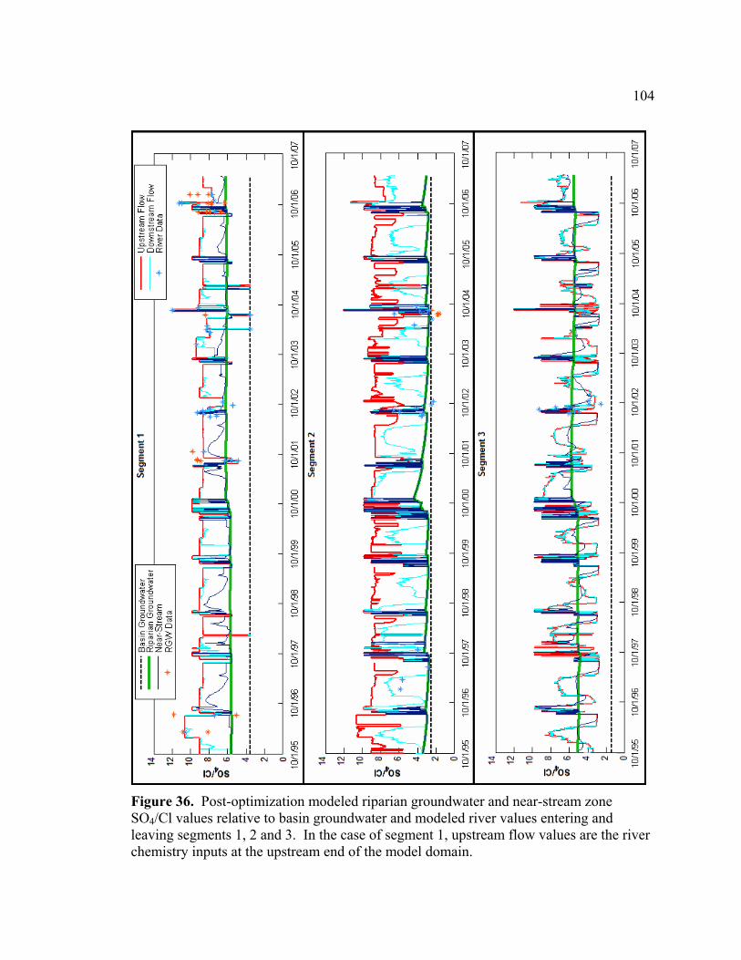
104
Figure 36. Post-optimization modeled riparian groundwater and near-stream zone SO4/Cl values relative to basin groundwater and modeled river values entering and leaving segments 1, 2 and 3. In the case of segment 1, upstream flow values are the river chemistry inputs at the upstream end of the model domain.

105
Figure 37. Post-optimization modeled riparian groundwater and near-stream zone SO4/Cl values relative to basin groundwater and modeled river values entering and leaving segments 4, 5 and 6.

106
Figure 38. Post-optimization modeled riparian groundwater and near-stream zone SO4/Cl values relative to basin groundwater and modeled river values entering and leaving segments 7, 8 and 9.

107
Figure 39. Percent monsoon floodwater in the riparian groundwater (top) and in river
baseflow (bottom) for each model segment. Median values are indicated by horizontal red lines, quartile ranges by blue boxes and range of values by black brackets. Black dots and text are mean values and red points show statistical outliers. Green asterisks indicate mixing model results from Baillie et al. (2007).

108
Figure 40. Cumulative flux during model time domain (10/1/95 to 4/23/07) for model
segments 1-6. Units for each flux are 107 m3.
Figure 41. Cumulative flux during model time domain (10/1/95 to 4/23/07) for model
segments 7-9. Units for each flux are 107 m3.

109
Figure 42. Mean annual basin groundwater (BGW Flux), evapotranspirative (ET), and
river recharge/groundwater discharge fluxes for each model segment during the model time domain (10/1/95 to 4/23/07). Change in riparian groundwater storage is omitted due to the three-to-four order of magnitude difference relative to these fluxes.

110
APPENDIX B: TABLES
LIST OF TABLES
Table 1: Hydrologic characteristics of vegetation condition classes (information from Leenhouts, et al)…………………………….……………....111 Table 2: Summary of model parameters and state variables .........................................112-113 Table 3: Vegetative cover data……………………………………………………………..114 Table 4: Basin groundwater flux requirements ……………………………………….…...114 Table 5: Data used to derive model river input chemistry …….. …..……………………...115 Table 6: Model base case paratmeter set .….….….…………………………...…………..116 Table 7: Sensitivity Analysis: Parameter ranges, units and rank of importance...................117 Table 8: Sensitivity Analysis: ‘Optimal’ parameter set... ….……………….....…….……..118 Table 9: Modeled riparian fluxes (cumulative)…………………………….….………...…119

111
Table 1. Hydrologic characteristics of vegetation-based condition class model (information from Stromberg et al. in Leenhouts, et al. (2005))
Flow Permanence Mean floodplain Ground-
Condition (%) groundwater depth (m) water Class fluctuation
2002 2003 2002 2003
(m) 1 48 17 2.5 3.5 1.8 2 78 ± 15 63 ± 21 2.5 ± 0.6 3.0 ± 0.9 0.9 ± 0.7 3 100 ± 0 98 ± 4 1.6 ± 0.5 1.7 ± 0.5 0.3 ± 0.0

112
Tab
le 2
a.
Sum
mar
y of
par
amet
ers i
mpo
rtant
in d
eter
min
ing
the
stat
e, a
nd th
us th
e be
havi
or, o
f the
mod
el.

113
Tab
le 2
b.
Sum
mar
y of
stat
e va
riabl
es im
porta
nt in
det
erm
inin
g th
e st
ate,
and
thus
the
beha
vior
, of t
he m
odel
.

114
Table 3. Proportion of land surface within 100 meters of main river channel covered by the four phreatophyte groups. Determined from land cover data collected and distributed by EPA/USDA-ARS (2003).
Segment Cottonwood Mesquite Sacaton Tamarisk
1 0.4225 0.0306 0.0158 0 2 0.3255 0.0192 0.2484 0 3 0.3594 0.0865 0.3197 0 4 0.3934 0.0687 0.2589 0 5 0.3125 0.0668 0.1702 0 6 0.2432 0.1730 0.0545 0 7 0.1482 0.3962 0.0473 0 8 0.1593 0.4314 0.0258 0 9 0.0315 0.4155 0.0561 0.1517
Table 4. Requirements for the magnitude and direction of basin groundwater flux (Qbgw)
with respect to riparian groundwater.
Parameter Requirement Qbgw(1) Must be positive and less than 0.183 m2/day Qbgw(2) Must be greater than 0.220 m2/day Qbgw(3) Must be greater than -0.619 m2/day and less than Qbgw(1) Qbgw(4) Must be greater than 0.252 m2/day Qbgw(5) Must be greater than 0.188 m2/day Qbgw(6) Must be greater than 0.120 m2/day Qbgw(7) Must be negative and greater than -0.474 m2/day Qbgw(8) Must be negative
Qbgw(9) Must be negative

115
n SO4 Cl SO4/Cl n δ18O δ2H Early Monsoon High Flow 2 21.32 2.87 7.42 3 -9.08 -63.2
Mid-Monsoon High Flow 0 - - - 3 -6.57 -41.9Late-Monsoon High Flow 4 26.75 3.20 8.09 7 -5.86 -39.4
Monsoon Low Flows 3 22.24 3.46 6.12 12 -7.30 -53.1Spring Floods 1 3.37 0.95 3.57 1 -7.00 -36.5
Spring Baseflow 4 86.58 9.99 8.76 23 -6.30 -47.8Autumn/Winter Baseflow 3 79.48 9.42 8.20 27 -6.74 -49.7
Table 5. Data used in deriving model input values for SO4/Cl, δ18O and δ2H
grouped by time of year and hydrograph condition (n= number of samples available for each group). n values for groups differ because all samples were analyzed for δ18O and δ2H but not for anion concentrations. Data is from the Palominas USGS gauge and was either retrieved from the USGS-NWIS database or unpublished data collected during the Baillie et al. (2007) study.

116
Table 6a. Segment-specific parameters for model base case.
Segment-Specific Parameters Qbgw Segment Surface Entrenchment (m2/day) Length (m) Elevation (m) (m)
Segment 1 0.005 4660 1288.44 1.68Segment 2 0.300 5975 1261.57 2.08Segment 3 -0.250 6000 1252.63 1.78Segment 4 0.280 6080 1233.62 2.04Segment 5 0.280 5200 1223.00 1.97Segment 6 0.120 4900 1213.21 2.03Segment 7 -0.300 4900 1200.00 2.29Segment 8 -0.350 4380 1186.01 2.70Segment 9 -0.400 4650 1150.46 1.54
Table 6b. Base case parameters for entire model domain.
Diffusivity 3090 m2/day Specific Yield 0.32
RGW Reservoir Width 100 m RGW Reservoir Depth (BLS) 10 m Near-stream zone volume 10 m2

117
Tab
le 7
. R
ange
s, un
its a
nd ra
nk o
f im
porta
nce
(for
hyd
rolo
gic
and
chem
ical
/isot
opic
syst
em st
ates
and
flux
es) f
or e
ach
of
the
21 p
aram
eter
s alte
red
durin
g on
e-at
-a-ti
me
sens
itivi
ty a
naly
sis.
*Th
e ab
senc
e of
impo
rtanc
e va
lue
and
rank
for a
giv
en
para
met
er in
dica
tes n
o se
nsiti
vity
of t
he o
utpu
t cla
ss to
any
per
turb
atio
n of
the
para
met
er.
**‘1σ’
rang
es u
sed
for b
asin
gr
ound
wat
er c
hem
istry
per
turb
atio
n w
ere
0.4‰
(δ18
O) a
nd 0
.4 (S
O4/C
l) (a
fter b
asin
gro
undw
ater
end
-mem
ber (
Bai
llie
et a
l.,
2007
)).

118
Table 8. ‘Optimal’ parameter set based on manual calibration. Segment length, entrenchment and land surface elevations were unchanged from the base case parameter set.
Segment-Specific Parameters Qbgw Segment Surface Entrenchment (m2/day) Length (m) Elevation (m) (m)
Segment 1 0.020 4660 1288.44 1.68 Segment 2 0.500 5975 1261.57 2.08 Segment 3 0.010 6000 1252.63 1.78 Segment 4 0.800 6080 1233.62 2.04 Segment 5 0.700 5200 1223.00 1.97 Segment 6 0.200 4900 1213.21 2.03 Segment 7 -0.600 4900 1200.00 2.29 Segment 8 -0.500 4380 1186.01 2.70 Segment 9 -0.400 4650 1150.46 1.54
Diffusivity 1760 m2/day
Specific Yield 0.16 RGW Reservoir Width 100 m
RGW Reservoir Depth (BLS) 10 m Near-stream zone volume 10 m2

119
Tab
le 9
. C
umul
ativ
e ba
sin
grou
ndw
ater
(Qbg
w),
evap
otra
nspi
rativ
e (E
T), a
nd ri
ver
rech
arge
/gro
undw
ater
dis
char
ge fl
uxes
for e
ach
mod
el se
gmen
t dur
ing
the
mod
el
time
dom
ain
(10/
1/95
to 4
/23/
07).
Rel
ativ
e pr
opor
tions
of e
ach
flux
occu
rrin
g in
th
e up
per ~
70%
of t
he m
odel
(seg
men
ts 1
-6) a
nd lo
wer
~30
% (s
egm
ents
7-9
) are
al
so sh
own
for c
ompa
rison
.

120
APPENDIX C: CONDITION SCORE BIOINDICATORS
Bioindicator Variables (from Stromberg et al., 2005) 1 - Number of 10-cm Fremont cottonwood + Goodding willow size classes in flood
plain 2 - Fremont cottonwood + Goodding willow basal area (m2/ha) 3 - Fremont cottonwood + Goodding willow relative basal area (%) 4 - Maximum vegetation height (m) in flood plain 5 - Shrublands cover in flood plain (%) 6 - Absolute cover of streamside hydric perennial herbs (%) 7 - Relative cover of streamside hydric perennial herbs (%) 8 - Absolute cover of streamside hydric herbs (%) 9 - Relative cover of streamside hydric herbs (%)

121
APPENDIX D: MODEL ENTRENCHMENT DEPTHS
EntrenchmentSegment (m)
1 1.68 2 2.08 3 1.78 4 2.04
5 1.97 6 2.03 7 2.29 8 2.70 9 1.54

122
APPENDIX E: PALOMINAS RIVER WATER QUALITY DATA River chemical/isotopic values at Palominas; basis for model input
δ18O δ2H Chloride Sulfate Data Source Date per mil per mil mg/L mg/L
USGS-NWIS 8/31/94 -5.42 -38.3 6.3 89 USGS-NWIS 12/15/94 -11.11 -83.8 7.9 90 USGS-NWIS 3/15/95 -8.25 -63.2 8.7 75 USGS-NWIS 6/21/95 -7.95 -59.5 USGS-NWIS 3/12/96 -7.42 -54.5 8.1 86 USGS-NWIS 7/15/96 -7.85 -53.9 3.1 23 USGS-NWIS 8/12/99 -6.03 -44.6 USGS-NWIS 8/26/99 -6.92 -50.4 USGS-NWIS 12/21/99 -7.10 -52.3 USGS-NWIS 1/26/00 -7.08 -51.5 USGS-NWIS 2/24/00 -6.88 -50.8 USGS-NWIS 3/28/00 -6.70 -49.4 USGS-NWIS 4/27/00 -5.34 -45.7 USGS-NWIS 6/28/00 -11.92 -86.4 USGS-NWIS 7/26/00 -6.88 -52.5 USGS-NWIS 10/3/00 -6.55 -48.6 USGS-NWIS 11/30/00 -7.39 -53.1 USGS-NWIS 12/21/00 -7.18 -52.5 USGS-NWIS 3/5/01 -6.94 -51.4 USGS-NWIS 3/28/01 -6.98 -50.0 USGS-NWIS 4/26/01 -6.91 -50.9 USGS-NWIS 6/1/01 -7.07 -52.9 USGS-NWIS 6/28/01 -7.00 -48.9 USGS-NWIS 7/26/01 -5.93 -39.6 USGS-NWIS 8/14/01 -5.96 -37.5 4 25.2 USGS-NWIS 8/15/01 -5.84 -38.6 2.91 14.1 USGS-NWIS 8/16/01 -6.47 -44.5 3.06 17.2 USGS-NWIS 8/24/01 -6.61 -46.2 USGS-NWIS 8/30/01 -6.53 -48.4 USGS-NWIS 9/27/01 -6.68 -48.9 USGS-NWIS 10/19/01 -6.46 -47.5 USGS-NWIS 11/29/01 -6.63 -49.0 USGS-NWIS 12/27/01 -6.84 -51.9 USGS-NWIS 1/30/02 -7.00 -50.8 USGS-NWIS 2/28/02 -6.72 -50.3 USGS-NWIS 3/28/02 -6.61 -48.8

123
APPENDIX E – continued
δ18O δ2H Chloride Sulfate Data Source Date per mil per mil mg/L mg/L
USGS-NWIS 5/1/02 -6.43 -47.7 USGS-NWIS 5/23/02 -6.20 -48.1 USGS-NWIS 6/27/02 -5.52 -45.0
S. Lemon Thesis 6/29/02 9.7 76.4 S. Lemon Thesis 7/4/02 10.5 75.8 S. Lemon Thesis 7/22/02 8.2 70.9 S. Lemon Thesis 7/30/02 3.6 33.8
USGS-NWIS 8/1/02 -8.60 -62.0 S. Lemon Thesis 8/12/02 4.1 35.7 S. Lemon Thesis 8/31/02 9.5 75.5 S. Lemon Thesis 9/20/02 10.5 57.3 S. Lemon Thesis 10/18/02 11.3 74.2
USGS-NWIS 12/23/02 -7.00 -52.2 USGS-NWIS 1/30/03 -6.71 -51.1 USGS-NWIS 2/10/03 -6.82 -50.3 USGS-NWIS 2/27/03 -6.89 -49.7 USGS-NWIS 3/27/03 -6.51 -49.0 USGS-NWIS 5/1/03 -6.12 -47.1 USGS-NWIS 11/25/03 -5.92 -44.4
BAILLIE THESIS 12/13/03 -6.26 -45 13.3 124.9 USGS-NWIS 2/3/04 -6.45 -49.2 USGS-NWIS 2/24/04 -6.53 -47.6
BAILLIE THESIS 3/7/04 -6.53 -47 7.8 61.5 BAILLIE THESIS 3/28/04 -6.19 -45 10.6 87.6
USGS-NWIS 4/2/04 -6.05 -45.3 BAILLIE THESIS 4/3/04 -7.00 -36 0.9 3.4 BAILLIE THESIS 4/24/04 -6.07 -46 13.5 111.2
USGS-NWIS 4/28/04 -6.08 -45.5 USGS-NWIS 6/3/04 -4.50 -40.0 USGS-NWIS 6/25/04 -8.40 -63.9
BAILLIE THESIS 7/15/04 -8.07 -60.8 3.1 11.1 USGS-NWIS 7/29/04 -7.20 -44.1
BAILLIE THESIS 8/5/04 -5.70 -45 1.7 10.5 BAILLIE THESIS 8/17/04 -5.53 -30.5 1.4 16.5
USGS-NWIS 8/31/04 -5.12 -40.8 BAILLIE THESIS 9/6/04 -7.42 -52 4.2 38.4
USGS-NWIS 10/7/04 -6.37 -48.5 USGS-NWIS 10/29/04 -6.64 -48.5
BAILLIE THESIS 11/2/04 -6.10 -47

124
APPENDIX E – continued
δ18O δ2H Chloride Sulfate Data Source Date per mil per mil mg/L mg/L
USGS-NWIS 11/30/04 -6.46 -46.2 USGS-NWIS 1/5/05 -7.20 -52.3 USGS-NWIS 2/4/05 -6.88 -49.3 USGS-NWIS 3/3/05 -6.95 -51.3 USGS-NWIS 4/8/05 -6.31 -47.5 USGS-NWIS 5/12/05 -6.09 -47.4 USGS-NWIS 6/9/05 -5.34 -44.6 USGS-NWIS 8/12/05 -9.11 -63.8 USGS-NWIS 9/9/05 -6.10 -36.8 This study 8/5/06 -7.46 -49.2 2.6 19.6 This study 10/7/06 -6.98 -46.7 6.7 74.2 This study 10/7/06 -6.78 -46.2 6.0 67.5 This study 10/27/06 -6.80 -49.5 7.8 58.2 This study 12/9/06 -6.96 -51.5 7.1 55.3

125
APPENDIX F: HEREFORD RUNOFF SAMPLE DATA
δ18O δ2H Chloride Sulfate Date per mil per mil mg/L mg/L
7/15/04 -12.5 -92 1.7 25.7

126
APPENDIX G: NEAR-RIPARIAN BASIN GROUNDWATER DATA Data for basin groundwater inputs grouped by model segment
Well δ18O δ2H Chloride Sulfate Segment Depth (ft)
Data Source Date per mil per mil mg/L mg/L
unknown USGS-NWIS 9/13/99 -7.96 -54.1 12.4 4.6 unknown USGS-NWIS 9/14/94 5.5 9.0
205 USGS-NWIS 6/24/96 -8.12 -57.8 16.0 11.0 unknown USGS-NWIS 9/14/99 -7.95 -55.3 4.2 8.5
117 USGS-NWIS 11/13/96 -6.75 -50.4 9.9 35.0 USGS-NWIS 7/3/01 -7.27 -51.1 USGS-NWIS 8/24/01 -7.25 -50.8 3.7 7.6 USGS-NWIS 10/18/01 -7.23 -50.9 3.5 8.9
1
203.5
BAILLIE THESIS 8/18/04 -7.26 -51.5 3.4 9.7 unknown BAILLIE THESIS 6/23/04 -8.6 -58.7 7.9 17.9 unknown BAILLIE THESIS 6/23/04 -8.6 -58.8 7.8 17.9
USGS-NWIS 2/24/55 20.0 50.0 2
475 USGS-NWIS 8/4/89 4.4 9.0
unknown BAILLIE THESIS 6/23/04 -9.6 -66.2 6.0 8.8 3 unknown USGS-NWIS 9/8/99 -8.42 -58.4 6.0 10.6 unknown USGS-NWIS 3/12/03 -8.11 -56.8
180 USGS-NWIS 3/28/95 -9.59 -67.9 4.2 9.3 4 300 USGS-NWIS 9/1/99 -8.39 -58.6 6.1 10.2
unknown USGS-NWIS 3/12/03 -8.6 -59.3 unknown USGS-NWIS 11/18/03 -7.92 -56.6 5 unknown USGS-NWIS 8/27/99 -8.39 -58.0 6.9 14.6
29 USGS-NWIS 7/5/01 -7.68 -52.2 1.5 4.5 6 90 USGS-NWIS 3/29/88 3.8 5.8

127
APPENDIX H: MODEL CODE
MODEL (MATLAB) CODE & RELATED MODEL FUNCTIONS
“Model”
%%%%%%%%%%%%%%%%%%%%%%%%%%%%%%%%%%%%%%%%%%%%%%%%
%%%%%%%%%%%%%%%% Stream-Aquifer Exchange Model %%%%%%%%%%%%%%
%%%%%%%%%%%%%%%%%%%%%%%%%%%%%%%%%%%%%%%%%%%%%%%%
clear all;close all;clc; %-------------------------------------------------------------------------% % Loading data and determining if there is % % inflow from side channels within the model domain % %-------------------------------------------------------------------------% load PAL_Riv.m; % Columns: day #, Q(cfs),Gage ht(m) PalQ=PAL_Riv(:,2)*86400/35.313378458; % Converts flow from cfs to m3/day N_data=length(PAL_Riv); % No. of timesteps ('t') load LSP_Riv.m; load Char_Riv.m; % Columns: day# (i.e. 39156); Q(cfs); gage height (m) CharQ=[Char_Riv(:,1) 86400*Char_Riv(:,2)/35.313378458]; load Tomb_Riv.m; TombQ=[Tomb_Riv(:,1) 86400*Tomb_Riv(:,2)/35.313378458]; load PALRivChem.m; load VegFracs.m; load Month.m; load DOY.m; load SegLength.m; % Length of each segment (in meters) N_seg=length(SegLength); [SideInflow,Chem.side]=InflowDays(N_data,PAL_Riv,Rel_Monsoon_Basin); % Calls fxn "InflowDays" (rows: days columns: segments) SideInflow=86400*SideInflow/35.313378458; %-------------------------------------------------------------------------% % Making blank matrices for later use % %-------------------------------------------------------------------------% Gage_ht=zeros(N_data,N_seg); % Rows: time / columns: segments Chem.bgw=zeros(1,4,N_seg); % Chemistry of basin groundwater additions will be static in time Chem.rgw=zeros(N_data,4,N_seg); % Columns: SO4,Cl,18O,2H (L to R) Chem.ns=zeros(N_data,4,N_seg); % " " " Chem.Rin=zeros(N_data,4,N_seg); % River chem ENTERING reach Chem.Rout=zeros(N_data,4,N_seg); % River chem LEAVING reach Chem.side=zeros(N_data,4,N_seg); % Chem of floodwater entering from side channels (made up) Q=zeros(N_data,4,N_seg); % Columns: 1. Qbgw(+/0/-, time-constant) % 2. Qrgw (+/0/-) % 3. Qsin(+/0)

128
% 4. Qsout(+/0) Vrgw=zeros(N_data,N_seg); % Volume of RGW tank per meter of river (m2) GWElev=zeros(N_data,N_seg); DailyET=zeros(N_data,N_seg); Grad=zeros(N_data,N_seg); RiverCond=zeros(N_data,N_seg); %-------------------------------------------------------------------------% % Initializing the system % %-------------------------------------------------------------------------% load Daquifer.m; % Diffusivity for each segment (units: m/day) D=Daquifer; % Changes name to 'D' D(:)=1760; % Post-SA diffustivity value load Qbgw.m; % Fluxes into each segment (UNITS: m2/day) load Surf_elev.m; % Land surface elevations (& top of RGW tank) load Entrenchment.m; % Distance b/w river bottom and land surface(m) load ZeroFlowStage.m; % Y-intercept in Q/Stage plots load InitGWElev.m; load ChemBgw.m; if Rel_Monsoon_Basin==1; ChemBgw(:,1)=0; ChemBgw(:,2)=1; end for z=1:N_seg; % Makes BGW chem into a 'plate' with front row as segment 1 chem Chem.bgw(1,:,z)=ChemBgw(z,:); Q(:,1,z)=Qbgw(z); if ChemBgw(z,2)>0; ChemBgwSO4_Cl(z)=ChemBgw(z,1)/ChemBgw(z,2); else ChemBgwSO4_Cl(z)=0; end end; % Chem.rgw(1,:,:)=Chem.bgw; % RGW at first time step is 100% BGW Chem.rgw(1,:,1)=[77.3691 13.8470 -7.2055 -49.0051]; Chem.rgw(1,:,2)=[24.1093 6.9422 -8.5643 -58.5449]; % These values are Chem.rgw(1,:,3)=[48.8458 9.6442 -7.6392 -51.6699]; % 10-1-06 values Chem.rgw(1,:,4)=[30.8479 15.4903 -8.4951 -58.5021]; % (day #4019) Chem.rgw(1,:,5)=[20.3332 7.0612 -8.0272 -54.9019]; % from a run with Chem.rgw(1,:,6)=[23.3436 24.9219 -7.9695 -53.8624]; % RGW chemistry Chem.rgw(1,:,7)=[34.9797 10.8888 -7.9002 -53.9805]; % same as BGW Chem.rgw(1,:,8)=[37.4821 10.9147 -7.8011 -53.1713]; % (8-15-07) Chem.rgw(1,:,9)=[37.8834 10.0809 -7.7536 -52.7299]; if Rel_Monsoon_Basin==1; Chem.rgw(1,1:2,1)=[82.1854 1.0000]; % 5th iteration results: Chem.rgw(1,1:2,2)=[29.3488 1.0000]; % All segments have converged Chem.rgw(1,1:2,3)=[69.4978 1.0000]; % to 3 decimal places Chem.rgw(1,1:2,4)=[19.7063 1.0000]; Chem.rgw(1,1:2,5)=[22.1006 1.0000]; Chem.rgw(1,1:2,6)=[37.8016 1.0000];

129
Chem.rgw(1,1:2,7)=[41.7695 1.0000]; Chem.rgw(1,1:2,8)=[45.8203 1.0000]; Chem.rgw(1,1:2,9)=[54.4789 1.0000]; end Chem.ns(1,:,:)=Chem.rgw(1,:,:); % NSZ at first time step is same as RGW Q(:,3,1)=PalQ; load PALRivChemData4.m; PALRivChemData=PALRivChemData4; if Rel_Monsoon_Basin==1; for t=1:length(PAL_Riv); if Month(t)>5 & Month(t)<11; PALRivChemData(t,1)=100; % Flow at PAL from June 1-Oct 31 is considered 100% floodwater PALRivChemData(t,2)=1; else PALRivChemData(t,1)=0; % Flow at PAL from June 1-Oct 31 is considered 0% floodwater PALRivChemData(t,2)=1; end end end Chem.Rin(:,1,1)=PALRivChemData(:,1); % SO4 Chem.Rin(:,2,1)=PALRivChemData(:,2); % Cl Chem.Rin(:,3,1)=PALRivChemData(:,3); % d18O Chem.Rin(:,4,1)=PALRivChemData(:,4); % d2H for seg=1:N_seg; if Qbgw(seg)>0; ReachChar(seg)=1; % + BGW discharge makes these GW-gaining reaches else ReachChar(seg)=2; % - BGW discharge makes these GW-losing reaches end; end; %-------------------------------------------------------------------------% % Parameters % %-------------------------------------------------------------------------% Sy=0.16; % Specific yield (assumed constant throughout entire domain) % **It is also assumed that there is no vadose zone storage Pars.Vns=10*Sy; % Volume of near-stream zone (channel + subsurface) RGW_width=100; % width of RGW tank is 100 m at all segments PorousTankWidth=RGW_width*Sy; % ---> multiply by specific yield so that water level changes are % for a porous medium and not for an "underground void"-type tank RGWDepth=10; % RGW tank depth Riv_bottom=Surf_elev-Entrenchment-ZeroFlowStage; RGW_bottom=Riv_bottom-RGWDepth+ZeroFlowStage; Vrgw_max=(Surf_elev-RGW_bottom)*RGW_width*Sy; for seg=1:9; GWElev(1,seg)=InitGWElev(seg); % initial GWElev & Vrgw x 9 segments Vrgw(1,seg)=(GWElev(1,seg)-RGW_bottom(seg))*PorousTankWidth; end;

130
%%%%%%%%%%%%%%%%%%%%%%%%%%%%%%%%%%%%%%%%%%%%% %%%%%%%%%%%%%%%%% MODEL CALCULATIONS %%%%%%%%%%%%%% %%%%%%%%%%%%%%%%%%%%%%%%%%%%%%%%%%%%%%%%%%%%% for t=1:N_data; % all times for seg=1:9; % all segments V_rgwPreET(t,seg)=Vrgw(t,seg)+Q(t,1,seg); % new RGW volume = initial volume + flux w.r.t. BGW (units: m2) % --> sign of Qgbw reflects gaining/losing if V_rgwPreET(t,seg)>Vrgw_max(seg); % ensuring bucket doesn't overflow after BGW addition V_rgwPreET(t,seg)=Vrgw_max(seg); GWElev(t,seg)=Surf_elev(seg); Q(t,1,seg)=V_rgwPreET(t,seg)-Vrgw(t,seg); end if Q(t,1,seg)<0 & Vrgw(t,seg)<abs(Q(t,1,seg)); V_rgwPreET(t,seg)=0; Q(t,1,seg)=-Vrgw(t,seg); end if ReachChar(seg)==1; % Calc chemical changes for GW-gaining reach New_SO4(t,seg)=ConcRecalc(Chem.bgw(1,1,seg),Chem.rgw(t,1,seg),... Qbgw(seg),Vrgw(t,seg)); % gives chem/iso values post BGW add'n New_Cl(t,seg)=ConcRecalc(Chem.bgw(1,2,seg),Chem.rgw(t,2,seg),... Qbgw(seg),Vrgw(t,seg)); % Vrgw(t,seg) is initial volume New_18O(t,seg)=ConcRecalc(Chem.bgw(1,3,seg),Chem.rgw(t,3,seg),... Qbgw(seg),Vrgw(t,seg)); New_2H(t,seg)=ConcRecalc(Chem.bgw(1,4,seg),Chem.rgw(t,4,seg),... Qbgw(seg),Vrgw(t,seg)); end; if ReachChar(seg)==2; % Calc chemical changes for GW-losing reach % no change in chemistry in RGW when losing w.r.t. BGW New_SO4(t,seg)=Chem.rgw(t,1,seg); New_Cl(t,seg)=Chem.rgw(t,2,seg); New_18O(t,seg)=Chem.rgw(t,3,seg); New_2H(t,seg)=Chem.rgw(t,4,seg); end; %----- ET removals (after BGW has been either added or subtracted) -----% DepthToGW(t,seg)=Surf_elev(seg)-GWElev(t,seg); DailyET(t,seg)=New_ETCalc(Month(t),GWElev(t,seg),Surf_elev(seg),... VegFracs(seg,1),VegFracs(seg,2),VegFracs(seg,3),VegFracs(seg,4),... DOY(t),seg); TotalET(t,seg)=DailyET(t,seg)*RGW_width; V_rgwPostET(t,seg)=V_rgwPreET(t,seg)-TotalET(t,seg); % Volume in RGW after ET removal = Vol before ET - ET volume GWElev_postET(t,seg)=RGW_bottom(seg)+V_rgwPostET(t,seg)/PorousTankWidth; % Elev. of water table = elev of bottom + water depth in RGW if Rel_Monsoon_Basin==1; PostET_SO4(t,seg)=New_SO4(t,seg); PostET_Cl(t,seg)=New_Cl(t,seg); % gives chemical signatures after ET (only SO4 and Cl change) else

131
PostET_SO4(t,seg)=ET_Recalc(V_rgwPreET(t,seg),V_rgwPostET(t,seg),... New_SO4(t,seg)); % chem. conc. after ET (only SO4 and Cl change) PostET_Cl(t,seg)=ET_Recalc(V_rgwPreET(t,seg),V_rgwPostET(t,seg),... New_Cl(t,seg)); end PostET_18O(t,seg)=New_18O(t,seg); PostET_2H(t,seg)=New_2H(t,seg); % ET does not fractionate, thus per mil values will not change Chem.rgw(t,1,seg)=PostET_SO4(t,seg); Chem.rgw(t,2,seg)=PostET_Cl(t,seg); Chem.rgw(t,3,seg)=PostET_18O(t,seg); Chem.rgw(t,4,seg)=PostET_2H(t,seg); %--------------------- end of ET calculations ---------------------------% %-------------------------------------------------------------------------% %-Adding surface flow to the river (if it enters within the model domain)-% %-------------------------------------------------------------------------% if SideInflow(t,seg)>0; % Adding flow if it enters the river from side channels below PAL for s=1:4; % Recalculates stream chemistry for the 4 species (SO4,Cl,18O,2H) Chem.Rin(t,s,seg)=ConcRecalc(Chem.side(t,s,seg),Chem.Rin(t,s,seg),... SideInflow(t,seg),Q(t,3,seg)); end; Q(t,3,seg)=SideInflow(t,seg)+Q(t,3,seg); % Adds side channel flow end; %-------------------------------------------------------------------------% % Determining if the river is gaining/neutral/losing and exchanging water % %-------------------------------------------------------------------------% Gage_ht(t,seg)=StageFromQ(Q(t,3,seg),seg); % Calc. river stage from discharge entering model segment Riv_Elev(t,seg)=Riv_bottom(seg)+Gage_ht(t,seg); % Elev. of river surface = elev of river bottom + gage ht if GWElev_postET(t,seg)==Riv_Elev(t,seg); % NO EXCHANGE if NO GRADIENT RiverCond(t,seg)=0; % River and aquifer do not interact w/o gradient Q(t,4,seg)=Q(t,3,seg); % ... meaning that Q out = Q into the reach Chem.Rout(t,:,seg)=Chem.Rin(t,:,seg); % ... and river chemistry doesn't change GW_Elev_final=GWElev_postET(t,seg); else % Calculating volume of water exchanged b/w river, NSZ and aquifer [RiverCond(t,seg),Q(t,4,seg),Chem.Rout(t,:,seg),Chem.ns(t,:,seg),... Chem.rgw(t,:,seg),GW_Elev_final,FinalVrgw(t,seg),Grad(t,seg)]=... RivAqNSZ(t,seg,Chem,D(seg),GWElev_postET(t,seg),Riv_Elev(t,seg),... RGW_width,Pars.Vns,SegLength(seg),V_rgwPostET(t,seg),Q(t,3,seg),... Riv_bottom(seg),RGW_bottom(seg),Gage_ht(t,seg),PorousTankWidth,... Sy,Vrgw_max(seg)); % The above function ("RivAqNSZ") calculates

132
% 1) Whether the river is gaining or losing RiverCond(t,seg) % 2) Outflow from the model segment at time = t Q(t,4,seg) % 3) Chemistry of RGW, NSZ and river AFTER exchange Chem.Rout,_.ns,_.rgw % 4) Final RGW (water table) elevation GW_Elev_final % 5) Final volume of RGW FinalVrgw(t,seg) % 6) Hydraulic gradient Grad(t,seg) end; %-------------------------------------------------------------------------% %-------- Initializing data for the next time step and/or segment --------% %-------------------------------------------------------------------------% Q(t,2,seg)=Q(t,4,seg)-Q(t,3,seg); % Discharge from/into RGW is Qout-Qin ----> (+ is gaining river) if seg<9; % Passing information from one SEGMENT to the next Q(t,3,seg+1)=Q(t,4,seg); % Qin to next segment equals Qout from current segment (same 't') Chem.Rin(t,:,seg+1)=Chem.Rout(t,:,seg); end; if t<N_data; % Passing information from one 't' to the next GWElev(t+1,seg)=GW_Elev_final; GW_Elev_final=[]; Vrgw(t+1,seg)=FinalVrgw(t,seg); % Initial Vrgw at next 't' is the final one for this 't' Chem.rgw(t+1,:,seg)=Chem.rgw(t,:,seg); % Initial RGW chemistry at next 't' is the final one for this 't' Chem.ns(t+1,:,seg)=Chem.ns(t,:,seg); % Initial NSZ chemistry at next 't' is the final one for this 't' end; end; end; disp('-----------------------Model Ran Successfully----------------------') %%%%%%%%%%%%%%%%%%%%%%%%%%%%%%%%%%%%%%%%%%%%% %%%%%%%%%%%%%%%%% END OF MODEL CALCULATIONS %%%%%%%%%% %%%%%%%%%%%%%%%%%%%%%%%%%%%%%%%%%%%%%%%%%%%%%

133
“ConcRecalc”
function [C_new]=ConcRecalc(Cin,Cprev,Vin,Vprev); % recalculates the concentration of a reservoir based on previous volume % and amount added from a second reservoir (& respective concentrations) Vtot=Vin+Vprev; C_new=(Cin*Vin+Cprev*Vprev)/Vtot;

134
“New_ETCalc”
function [ETforToday]=New_ETCalc(Month,GWElev,Surf_elev,FracCot,... FracMesq,FracSac,FracTam,DOY,seg); % Function calculating the amount of ET lost for a given depth to GW, % season and combination of species as plant cover DepthToGW=Surf_elev-GWElev; % (m) ETforToday=0; % ET=0 unless specified differently below %%%%%%%%%%%%%%%%%%%%%%%%%%%%%%%%%%%%%%%%%%%%% %%%%%%%%%%%%%%%%% ET for spring (April-May) %%%%%%%%%%%%%%% %%%%%%%%%%%%%%%%%%%%%%%%%%%%%%%%%%%%%%%%%%%%% if Month<6 & Month>3; if DepthToGW<=0.75 & DepthToGW>=0; % WT is 0 to 0.75 m BLS MesqET=0; % mm/day CotET=FracCot*(1.904*DepthToGW); % mm/day TamET=0; % mm/day SacET=FracSac*(1.4653*DepthToGW); % mm/day Evap=-4.5749*DepthToGW+4.5749; % mm/day end if DepthToGW>0.75 & DepthToGW<=1; % WT is 0.75 to 1 m BLS MesqET=0; CotET=FracCot*(4.488*DepthToGW-1.938); TamET=0; SacET=FracSac*(4.3959*DepthToGW-2.1979); Evap=-4.5749*DepthToGW+4.5749; end if DepthToGW>1 & DepthToGW<=1.5; % WT is 1 to 1.5 m BLS MesqET=0; CotET=FracCot*(0.612*DepthToGW+1.938); TamET=0; SacET=FracSac*(0.1465*DepthToGW+2.0514); Evap=0; end if DepthToGW>1.5 & DepthToGW<=2; % WT is 1.5 to 2 m BLS MesqET=0; CotET=FracCot*2.856; TamET=0; SacET=FracSac*2.2712; Evap=0; end if DepthToGW>2 & DepthToGW<=3; % WT is 2 to 3 m BLS MesqET=FracMesq*(1.36*DepthToGW-2.72); CotET=FracCot*2.856; TamET=FracTam*(1.36*DepthToGW-2.72); SacET=FracSac*(-0.0733*DepthToGW+2.4177); Evap=0; end if DepthToGW>3 & DepthToGW<=4; % WT is 3 to 4 m BLS

135
MesqET=FracMesq*(1.53*DepthToGW-3.23); CotET=FracCot*(-1.428*DepthToGW+7.14); TamET=FracTam*(1.768*DepthToGW+3.944); SacET=FracSac*(-1.099*DepthToGW+5.4948); Evap=0; end if DepthToGW>4 & DepthToGW<=5; % WT is 4 to 5 m BLS MesqET=FracMesq*2.89; CotET=FracCot*(-1.088*DepthToGW+5.78); TamET=FracTam*(0.136*DepthToGW+2.584); SacET=FracSac*(-1.099*DepthToGW+5.4948); Evap=0; end if DepthToGW>5 & DepthToGW<=6; % WT is 5 to 6 m BLS MesqET=FracMesq*2.89; CotET=FracCot*(-0.34*DepthToGW+2.04); TamET=FracTam*3.264; SacET=0; Evap=0; end if DepthToGW>6 & DepthToGW<=7; % WT is 6 to 7 m BLS MesqET=FracMesq*2.89; CotET=0; TamET=FracTam*3.264; SacET=0; Evap=0; end if DepthToGW>7 & DepthToGW<=8; % WT is 7 to 8 m BLS MesqET=FracMesq*2.89; CotET=0; TamET=FracTam*(-0.204*DepthToGW+4.692); SacET=0; Evap=0; end if DepthToGW>8 & DepthToGW<=9; % WT is 8 to 9 m BLS MesqET=FracMesq*(0.0272*DepthToGW+2.6724); CotET=0; TamET=FracTam*(-1.7*DepthToGW+16.66); SacET=0; Evap=0; end if DepthToGW>9 & DepthToGW<=10; % WT is 9 to 10 m BLS MesqET=FracMesq*2.9172; CotET=0; TamET=FracTam*(-1.36*DepthToGW+13.6); SacET=0; Evap=0; end if DepthToGW>10 & DepthToGW<=11; % WT is 10 to 11 m BLS MesqET=2.9172;

136
CotET=0; TamET=0; SacET=0; Evap=0; end if DepthToGW>11 & DepthToGW<=12; % WT is 11 to 12 m BLS MesqET=FracMesq*(-0.5372*DepthToGW+8.8264); CotET=0; TamET=0; SacET=0; Evap=0; end if DepthToGW>12 & DepthToGW<=13; % WT is 12 to 13 m BLS MesqET=FracMesq*(-0.68*DepthToGW+10.54); CotET=0; TamET=0; SacET=0; Evap=0; end if DepthToGW>13 & DepthToGW<=14; % WT is 13 to 14 m BLS MesqET=FracMesq*(-1.7*DepthToGW+23.8); CotET=0; TamET=0; SacET=0; Evap=0; end if DepthToGW>14; % WT is more than 14 m BLS MesqET=0; CotET=0; TamET=0; SacET=0; Evap=0; end if seg==1; % segment-specific ET-smoothing parameters SFD=66.15;Shift=92;Warp=3.6; end if seg==2; SFD=66.15;Shift=92;Warp=3.6; end if seg==3; SFD=64;Shift=92;Warp=3.6; end if seg==4; SFD=66.15;Shift=92;Warp=3.701; end if seg==5; SFD=66.15;Shift=92;Warp=3.701; end if seg==6; SFD=66.15;Shift=92;Warp=3.701;

137
end if seg==7; SFD=62;Shift=92;Warp=3.5; end if seg==8; SFD=64.2;Shift=92;Warp=3.6; end if seg==9; SFD=66;Shift=92;Warp=3.69; end ETforToday=(CotET+MesqET+SacET+TamET+Evap)/1000; % converts to m/day ETforToday=ETforToday*Warp*sin((DOY-Shift)/SFD)*(365-DOY)/365; end %%%%%%%%%%%%%%%%%%%%%%%%%%%%%%%%%%%%%%%%%%%%%%
% %%%%%%%%%%%%%%%% ET for summer (June-Sept)
%%%%%%%%%%%%%%%%% %%%%%%%%%%%%%%%%%%%%%%%%%%%%%%%%%%%%%%%%%%%%%%
% if Month<10 & Month>5; if DepthToGW<=0.75 & DepthToGW>=0; % WT is 0 to 0.75 m BLS MesqET=0; % mm/day CotET=FracCot*(2.8*DepthToGW); % mm/day TamET=0; % mm/day SacET=FracSac*(2.1548*DepthToGW); % mm/day Evap=-6.7278*DepthToGW+6.7278; % mm/day end if DepthToGW>0.75 & DepthToGW<=1; % WT is 0.75 to 1 m BLS MesqET=0; CotET=FracCot*(6.6*DepthToGW-2.85); TamET=0; SacET=FracSac*(6.4645*DepthToGW-3.2323); Evap=-6.73*DepthToGW+6.73; end if DepthToGW>1 & DepthToGW<=1.5; % WT is 1 to 1.5 m BLS MesqET=0; CotET=FracCot*(0.9*DepthToGW+2.85); TamET=0; SacET=FracSac*(0.2155*DepthToGW+3.0168); Evap=0; end if DepthToGW>1.5 & DepthToGW<=2; % WT is 1.5 to 2 m BLS MesqET=0; CotET=FracCot*4.2; TamET=0; SacET=FracSac*3.34; Evap=0; end if DepthToGW>2 & DepthToGW<=3; % WT is 2 to 3 m BLS MesqET=FracMesq*(2*DepthToGW-4);

138
CotET=FracCot*4.2; TamET=FracTam*(2*DepthToGW-4); SacET=FracSac*(-0.1077*DepthToGW+3.5555); Evap=0; end if DepthToGW>3 & DepthToGW<=4; % WT is 3 to 4 m BLS MesqET=FracMesq*(2.25*DepthToGW-4.75); CotET=FracCot*(-2.1*DepthToGW+10.5); TamET=FracTam*(2.6*DepthToGW+5.8); SacET=FracSac*(-1.6161*DepthToGW+8.0806); Evap=0; end if DepthToGW>4 & DepthToGW<=5; % WT is 4 to 5 m BLS MesqET=FracMesq*4.25; CotET=FracCot*(-1.6*DepthToGW+8.5); TamET=FracTam*(0.2*DepthToGW+3.8); SacET=FracSac*(-1.6161*DepthToGW+8.0806); Evap=0; end if DepthToGW>5 & DepthToGW<=6; % WT is 5 to 6 m BLS MesqET=FracMesq*4.25; CotET=FracCot*(-0.5*DepthToGW+3); TamET=FracTam*4.8; SacET=0; Evap=0; end if DepthToGW>6 & DepthToGW<=7; % WT is 6 to 7 m BLS MesqET=FracMesq*4.25; CotET=0; SacET=0; TamET=FracTam*4.8; Evap=0; end if DepthToGW>7 & DepthToGW<=8; % WT is 7 to 8 m BLS MesqET=FracMesq*4.25; CotET=0; SacET=0; TamET=FracTam*(-0.3*DepthToGW+6.9); Evap=0; end if DepthToGW>8 & DepthToGW<=9; % WT is 8 to 9 m BLS MesqET=FracMesq*(0.04*DepthToGW+3.93); CotET=0; SacET=0; TamET=FracTam*(-2.5*DepthToGW+24.5); Evap=0; end if DepthToGW>9 & DepthToGW<=10; % WT is 9 to 10 m BLS MesqET=FracMesq*4.29; CotET=0;

139
SacET=0; TamET=FracTam*(-2*DepthToGW+20); Evap=0; end if DepthToGW>10 & DepthToGW<=11; % WT is 10 to 11 m BLS MesqET=4.29; CotET=0; TamET=0; SacET=0; Evap=0; end if DepthToGW>11 & DepthToGW<=12; % WT is 11 to 12 m BLS MesqET=FracMesq*(-0.79*DepthToGW+12.98); CotET=0; TamET=0; SacET=0; Evap=0; end if DepthToGW>12 & DepthToGW<=13; % WT is 12 to 13 m BLS MesqET=FracMesq*(-1*DepthToGW+15.5); CotET=0; TamET=0; SacET=0; Evap=0; end if DepthToGW>13 & DepthToGW<=14; % WT is 13 to 14 m BLS MesqET=FracMesq*(-2.5*DepthToGW+35); CotET=0; TamET=0; SacET=0; Evap=0; end if DepthToGW>14; % WT is more than 14 m BLS MesqET=0; CotET=0; TamET=0; SacET=0; Evap=0; end if seg==1; SFD=76;Shift=92;Warp=2.679; end if seg==2; SFD=76;Shift=92;Warp=2.679; end if seg==3; SFD=76;Shift=92;Warp=2.78; end if seg==4; SFD=84;Shift=88.5;Warp=2.9;

140
end if seg==5; SFD=73.7;Shift=91;Warp=2.68; end if seg==6; SFD=74;Shift=93;Warp=2.8; end if seg==7; SFD=75;Shift=91;Warp=2.68; end if seg==8; SFD=76;Shift=89;Warp=2.68; end if seg==9; SFD=76;Shift=105;Warp=2.679; end ETforToday=(CotET+MesqET+SacET+TamET+Evap)/1000; % converts to m/day ETforToday=ETforToday*Warp*sin((DOY-Shift)/SFD)*(365-DOY)/365; end %%%%%%%%%%%%%%%%%%%%%%%%%%%%%%%%%%%%%%%%%%% %%%%%%%%%%%%%%%%% ET for autumn (Oct-Nov) %%%%%%%%%%%%% %%%%%%%%%%%%%%%%%%%%%%%%%%%%%%%%%%%%%%%%%%% if Month<12 & Month>9; if DepthToGW<=0.75 & DepthToGW>=0; % WT is 0 to 0.75 m BLS MesqET=0; CotET=FracCot*(0.4467*DepthToGW); TamET=0; SacET=FracSac*(0.9355*DepthToGW); Evap=-4.29*DepthToGW+4.29; end if DepthToGW>0.75 & DepthToGW<=1; % WT is 0.75 to 1 m BLS MesqET=0; CotET=FracCot*(1.0529*DepthToGW-0.4546); TamET=0; SacET=FracSac*(2.8065*DepthToGW-1.4032); Evap=-4.29*DepthToGW+4.29; end if DepthToGW>1 & DepthToGW<=1.5; % WT is 1 to 1.5 m BLS MesqET=0; CotET=FracCot*(0.1636*DepthToGW+0.4346); TamET=0; SacET=FracSac*(0.0935*DepthToGW+1.3097); Evap=0; end if DepthToGW>1.5 & DepthToGW<=2; % WT is 1.5 to 2 m BLS MesqET=0; CotET=FracCot*0.68; TamET=0; SacET=FracSac*1.45; Evap=0;

141
end if DepthToGW>2 & DepthToGW<=3; % WT is 2 to 3 m BLS MesqET=FracMesq*(0.6867*DepthToGW-1.3734); CotET=FracCot*0.68; TamET=FracTam*(0.8333*DepthToGW+1.6667); SacET=FracSac*(-0.0468*DepthToGW+1.5435); Evap=0; end if DepthToGW>3 & DepthToGW<=4; % WT is 3 to 4 m BLS MesqET=FracMesq*(0.7726*DepthToGW-1.631); CotET=FracCot*(-0.345*DepthToGW+1.715); TamET=FracTam*(1.0833*DepthToGW-2.4167); SacET=FracSac*(-0.7016*DepthToGW+3.5081); Evap=0; end if DepthToGW>4 & DepthToGW<=5; % WT is 4 to 5 m BLS MesqET=FracMesq*1.4593; CotET=FracCot*(-0.2552*DepthToGW+1.356); TamET=FracTam*(0.0833*DepthToGW+1.5833); SacET=FracSac*(-0.7016*DepthToGW+3.5081); Evap=0; end if DepthToGW>5 & DepthToGW<=6; % WT is 5 to 6 m BLS MesqET=FracMesq*1.4593; CotET=FracCot*(-0.0798*DepthToGW+0.4786); TamET=FracTam*2; SacET=0; Evap=0; end if DepthToGW>6 & DepthToGW<=7; % WT is 6 to 7 m BLS MesqET=FracMesq*1.4593; CotET=0; SacET=0; TamET=FracTam*2; Evap=0; end if DepthToGW>7 & DepthToGW<=8; % WT is 7 to 8 m BLS MesqET=FracMesq*1.4593; CotET=0; SacET=0; TamET=FracTam*(-0.125*DepthToGW+2.875); Evap=0; end if DepthToGW>8 & DepthToGW<=9; % WT is 8 to 9 m BLS MesqET=FracMesq*(0.0207*DepthToGW+1.2935); CotET=0; SacET=0; TamET=FracTam*(-1.0417*DepthToGW+10.208); Evap=0; end

142
if DepthToGW>9 & DepthToGW<=10; % WT is 9 to 10 m BLS MesqET=FracMesq*1.48; CotET=0; SacET=0; TamET=FracTam*(-0.8333*DepthToGW+8.3333); Evap=0; end if DepthToGW>10 & DepthToGW<=11; % WT is 10 to 11 m BLS MesqET=FracMesq*1.48; CotET=0; TamET=0; SacET=0; Evap=0; end if DepthToGW>11 & DepthToGW<=12; % WT is 11 to 12 m BLS MesqET=FracMesq*(-0.2782*DepthToGW+4.5406); CotET=0; TamET=0; SacET=0; Evap=0; end if DepthToGW>12 & DepthToGW<=13; % WT is 12 to 13 m BLS MesqET=FracMesq*(-0.3434*DepthToGW+5.3221); CotET=0; TamET=0; SacET=0; Evap=0; end if DepthToGW>13 & DepthToGW<=14; % WT is 13 to 14 m BLS MesqET=FracMesq*(-0.8584*DepthToGW+12.018); CotET=0; TamET=0; SacET=0; Evap=0; end if DepthToGW>14; % WT is more than 14 m BLS MesqET=0; CotET=0; TamET=0; SacET=0; Evap=0; end if seg==1; SFD=76;Shift=92;Warp=15.73; end if seg==2; SFD=77;Shift=91;Warp=10; end if seg==3; SFD=76;Shift=92;Warp=10;
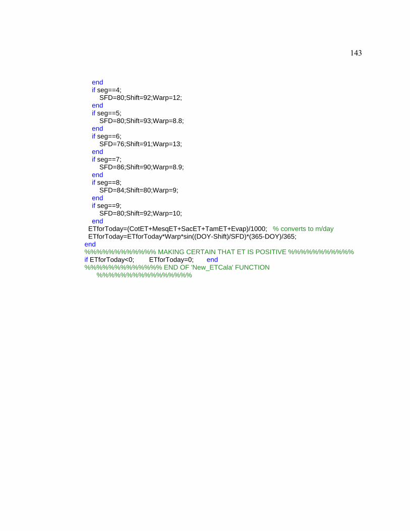
143
end if seg==4; SFD=80;Shift=92;Warp=12; end if seg==5; SFD=80;Shift=93;Warp=8.8; end if seg==6; SFD=76;Shift=91;Warp=13; end if seg==7; SFD=86;Shift=90;Warp=8.9; end if seg==8; SFD=84;Shift=80;Warp=9; end if seg==9; SFD=80;Shift=92;Warp=10; end ETforToday=(CotET+MesqET+SacET+TamET+Evap)/1000; % converts to m/day ETforToday=ETforToday*Warp*sin((DOY-Shift)/SFD)*(365-DOY)/365; end %%%%%%%%%%%% MAKING CERTAIN THAT ET IS POSITIVE %%%%%%%%%%% if ETforToday<0; ETforToday=0; end %%%%%%%%%%%%% END OF 'New_ETCala' FUNCTION
%%%%%%%%%%%%%%%%

144
“ET_Recalc”
function [NewConc]=ET_Recalc(V_rgwPreET,V_rgwPostET,Old_Conc); NewConc=Old_Conc*V_rgwPreET/V_rgwPostET; % recalculates SO4 and Cl concentrations in RGW after removal of % water via ET (which is assumed not to fractionate isotopically)

145
“StageFromQ” function [Stage]=StageFromQ(Q,seg); % 'StageFromQ' is a function that determines the average river stage (m) % from the discharge (m3/day) coming into any segment of the river %%%%%%%%%%%%%%%% CURVE PARAMETERS
%%%%%%%%%%%%%%%%%%% if seg==1; % Q/Stage relationship based on PAL data % Coeff=1728000; x_int=.9; exp=2.05;% PAL transect data (J. Leenhouts) Coeff=2100000; x_int=.7; exp=1.8; % based on entire PAL gage record end; if seg==2; % Q/Stage relationship based on KOL data Coeff=518400; x_int=1.5; exp=2.8; end; if seg==3; % Q/Stage relationship based on HUN data Coeff=604800; x_int=.9; exp=3.4; end; if seg==4; % Q/Stage relationship based on COT data Coeff=518400; x_int=1.8; exp=2.9; end; if seg==5; % Q/Stage relationship based on LSP data Coeff=181440; x_int=.2; exp=3.3; end; if seg==6; % Q/Stage relationship based on CHAR gage data Coeff=950400; x_int=.5; exp=2.54; end; if seg==7; % Q/Stage relationship based on CHM data Coeff=2592000; x_int=.7; exp=2.4; end; if seg==8; % Q/Stage relationship based on FBK data Coeff=1728000; x_int=.5; exp=2.4; end; if seg==9; % Q/Stage relationship based on CON data Coeff=1123200; x_int=.6; exp=3; end; %--------------------------- ACTUAL CALCULATION --------------------------- Stage=x_int+(Q/Coeff)^(1/exp); %----------------------- END OF FUNCTION 'StageFromQ' ---------------------

146
“RivAqNSZ” function [RiverCond,Q_out,ChemRout,Chemns,Chemrgw,GW_Elev_final,... V_rgwFinal,Grad]=RivAqNSZ(t,seg,Chem,D,GW_Elev,Riv_Elev,RGW_width,... Vnsz,SegLength,V_rgw_i,Q_in,Riv_bottom,RGW_bottom,Gage_ht_i,... PorousTankWidth,Sy,Vrgw_max); % 'RivAqNSZ' is a function determining the amount and direction of water % exchanged b/w the river, NSZ and RGW... AFTER IT HAS BEEN DETERMINED % THAT EXCHANGE HAPPENS (i.e. gradient is non-zero) % -->All volumes and river flux (q) is for one meter of stream length % INPUTS: % t = time step number (i.e. 4002) % seg = stream segment # % Chem = structure with ch0.emistry of ALL SEGMENTS AT ALL TIMES % D = diffusivity value of THIS segment % GW_Elev = GW elevation at start % Riv_Elev = river elevation at start % RGW_width = width of bucket (constant) % PorousTankWidth=Width of empty tank needed to simulate mixing volume % of a porous tank of RGW width (i.e. porosity x RGW width) % Vnsz = volume at this time step % SegLength = length of segment (in meters) % V_rgw_i = initial volume of RGW tank--before Riv/NSZ/Aq interaction % Q_in = river discharge coming into the segment % Riv_bottom = elevation of river bottom % RGW_bottom = elevation of RGW bottom % Gage_ht_i = river stage pre-exchange w/ RGW % OUTPUTS: % RiverCond = whether it's gaining (1) or losing (-1) % Q_out = discharge out of segment 'seg' at time 't' % ChemRout = 1x4 array of concentrations leaving river segment % Chemns = 1x4 array of NSZ chem AFTER exchange % Chemrgw = 1x4 array of RGW chem AFTER exchange % GW_Elev = elevation of water table in RGW AFTER exchange % Riv_Elev = elevation of river surface AFTER exchange % V_rgwFinal = volume of RGW AFTER exchange %%%%%%%%%%%%%%%%%%%%%%%%%%%%% INITIALIZING %%%%%%%%%% ChemRin=Chem.Rin(t,:,seg); ChemNSZi=Chem.ns(t,:,seg); Chemrgw=Chem.rgw(t,:,seg); ChemNSZf=zeros(1,4); %%%%%%%%%%%%%%%%%%%%%%%%%%%%% WATER BALANCE %%% Grad=(GW_Elev-Riv_Elev)/(0.5*RGW_width); % Hydraulic gradient: dh/dl---> NEGATIVE when river is LOSING T=D*Sy; % Diffusivity [m2/day] x Specific Yield [-] = T [m2/day] q=T*Grad; % Calc. flux per meter of river (+: gaining RIVER, -: losing)--(m2/day) V_rgwFinal=V_rgw_i-q; % Length-specific volume of RGW tank (m2) Q=q*SegLength;

147
% Volume of water added/lost along ENTIRE REACH ('SegLength' in meters) Q_out=Q_in+Q; % Volume of streamflow leaving the model section %------------------ Making sure water doesn't flow uphill ----------------- GW_Elev_postEx=RGW_bottom+(V_rgwFinal/PorousTankWidth); if q<0 & GW_Elev_postEx>Riv_Elev; % in losing conditions, water won't flow 'uphill' into RGW res. GW_Elev_postEx=Riv_Elev; V_rgwFinal=(GW_Elev_postEx-RGW_bottom)*PorousTankWidth; q=V_rgw_i-V_rgwFinal; Q=q*SegLength; Q_out=Q_in+Q; V_rgwFinal=V_rgw_i-q; % Length-specific volume of RGW tank (m2) end if q>0 & GW_Elev_postEx<Riv_Elev; % in gaining conditions, water won't flow 'uphill' into river GW_Elev_postEx=Riv_Elev; V_rgwFinal=(GW_Elev_postEx-RGW_bottom)*PorousTankWidth; q=V_rgw_i-V_rgwFinal; Q=q*SegLength; % Volume added/lost along the entire reach Q_out=Q_in+Q; % Streamflow volume leaving model section V_rgwFinal=V_rgw_i-q; % Length-specific volume of RGW tank (m2) end %-------------------------------------------------------------------------- if V_rgwFinal>Vrgw_max; % disallows RGW bucket from holding more than it's maximum volume V_rgwFinal=Vrgw_max; q=V_rgw_i-Vrgw_max; % must be NEGATIVE since river HAS to be losing to fill up RGW tank Q=q*SegLength; Q_out=Q_in+Q; V_rgwFinal=V_rgw_i-q; end if Q_out<0; % Making sure streamflow is either 0 or + (when river drys up) Q_out=0; Q=-Q_in; % Vol of water lost = volume in (when drys up) q=Q/SegLength; V_rgwFinal=V_rgw_i-q; end; if q<0; Q=-q*SegLength; % Makes 'Q' a positive quantity regardless of flux direction, % BUT...sign of 'q' still indicates direction end %-------------------------------------------------------------------------% %% Chemistry of the river & RGW does not change when the river is neutral % %-------------------------------------------------------------------------% if q==0; RiverCond=0; ChemRout=ChemRin;

148
ChemNSZf=ChemNSZi; GW_Elev_final=GW_Elev; V_rgwFinal=V_rgw_i; end; %%%%%%%%%%%%%%%%%%%%%%%%%%%%%%%%%%%%%%%%%%%%% %%%%%%%%%% Determining chemistry of the river & RGW %%%%%%%%%%%%% %%%%%%%%%%%%%%%%%%%%%%%%%%%%%%%%%%%%%%%%%%%%% if q>0; % RIVER IS GAINING RiverCond=1; if q<Vnsz; % when flux to river is LESS than NSZ volume, % all additions to streamflow come from NSZ for comp=1:4; % Calc. for 4 diff. chemical species (per meter of river) ChemNSZf(comp)=((Vnsz-q)*ChemNSZi(comp)+q*Chemrgw(comp))/Vnsz; % final NSZ chemistry if Q_out>0; % When river is flowing ChemRout(comp)=(Q_in*ChemRin(comp)+Q*ChemNSZi(comp))/Q_out; % final river chemistry else % When river has no flow ChemRout(comp)=ChemNSZf(comp); % Need to define river chem. when there is no flow??? end end; else % when flux to river is greater or equal to volume of NSZ, % some add'ns to streamflow come from NSZ and some from RGW Q_fromNSZ=Vnsz*SegLength; Q_fromRGW=Q-Q_fromNSZ; % Vol. from RGW = flux to river - NSZ vol. for comp=1:4; % Calc. for 4 diff. species if Q_out>0; ChemRout(comp)=(Q_in*ChemRin(comp)+Q_fromNSZ*ChemNSZi(comp)+... Q_fromRGW*Chemrgw(comp))/Q_out; % Adds NSZ and RGW water to the river else % Useless loop ChemRout(comp)=0; end ChemNSZf(comp)=Chemrgw(comp); % When NSZ empties, replaced entirely w. water from RGW end; end; end; %---------------------------- RIVER IS LOSING ----------------------------% if q<0; RiverCond=-1; ChemRout=ChemRin; % When river is losing, river chem doesn't change q_ab=-q; % Makes flux a positive number if q_ab<Vnsz; % when recharge < NSZ volume, all streamflow goes into NSZ for comp=1:4; % Calc. for 4 diff. species ChemNSZf(comp)=((Vnsz-q_ab)*ChemNSZi(comp)+q_ab*ChemRin(comp))/Vnsz; % river losses go into NSZ... Chemrgw(comp)=(q_ab*ChemNSZi(comp)+V_rgw_i*Chemrgw(comp))/V_rgwFinal;

149
% ... & NSZ losses go into RGW end; else % when recharge is >= volume of NSZ, some streamflow goes % into NSZ (+ some NSZ water goes into RGW) for comp=1:4; % Calc. for 4 diff. species q_fromRiver=q_ab-Vnsz; Chemrgw(comp)=(V_rgw_i*Chemrgw(comp)+q_fromRiver*ChemRin(comp)+... Vnsz*ChemNSZi(comp))/V_rgwFinal; ChemNSZf(comp)=ChemRin(comp); end; end; end; %-------------------------FINALIZING VARIABLES----------------------------% GW_Elev_final=RGW_bottom+(V_rgwFinal/PorousTankWidth); Chemns=ChemNSZf; ChemNSZf=[]; %---------------------- END OF FUNCTION 'RivAqNSZ' ------------------------

150
REFERENCES
Baillie MN, Hogan JF, Ekwurzel B, Wahi AK, Eastoe CJ. 2007. Quantifying water sources to a semiarid riparian ecosystem, San Pedro River, Arizona. J. Geophys. Res., 112, G03S02.
Baird KJ, Stromberg JC, Maddock T. 2005. Linking riparian dynamics and groundwater: An ecohydrologic approach to modeling groundwater and riparian vegetation. Environ Manage 36(4):551-64.
Brooks PD, and Lemon MM. 2007. Spatial variability in dissolved organic matter and inorganic nitrogen concentrations in a semiarid stream, San Pedro River, Arizona, J. Geophys. Res., 112, G03S05.
Chanat JG and Hornberger GM. 2003. Modeling catchment-scale mixing in the near-stream zone-implications for chemical and isotopic hydrograph separation. Geophys Res Lett 30(2).
Coplen TB. 1995. Reporting of stable carbon, hydrogen and oxygen abundances, Vienna, International Atomic Energy Agency, IAEA Tecdoc, 825, 31-34.
Cox WB and Stephens DB. 1988. Field study of ephemeral stream-aquifer interaction. Proceedings of the FOCUS Conference on Southwestern Ground Water Issues. National Water Well Association, Dublin OH.1988.p 337-358, 11 Fig.
Craig H. 1957. Isotopic standards for carbon and oxygen and correction factors for mass spectrometric analysis of carbon dioxide, Geochim. Cosmochim. Acta., 12, 133-149.
Freeze RA and Cherry JA. 1979. Groundwater, Prentice-Hall, Englewood Cliffs, NJ. 604 p.
Gehre M, Hoefling R, Kowski P, Strauch G. 1996. Sample preparation device for quantitative hydrogen isotope analysis using chromium metal, Analytical Chemistry, 68, 4414-4417.
Gillespie JB and Perry CA. 1988. Channel infiltration along the Pawnee River and its tributaries, West Central Kansas. Available from Books and Open File Report Section, USGS Box 25425. USGS Water Resources Investigations Report 88-4055:5 ref.

151
Gonfiantini R. 1978. Standards for stable isotope measurements in natural compounds, Nature, 271, 534-536.
Goodrich DC, Lane LJ, Shillito RM, Miller SN, Syed KH, Woolhiser DA. 1997. Linearity of basin response as a function of scale in a semiarid watershed. Water Resour Res 33(12):2951-65.
Goodrich DC, Williams DG, Unkrich CL, Hogan JF, Scott RL, Hultine KR, Pool D, Coes AL, Miller S. 2004. Comparison of methods to estimate ephemeral channel recharge, Walnut Gulch, San Pedro River Basin, Arizona, in Groundwater Recharge in a Desert Environment: the Southwestern United States, edited by J.F. Hogan, F.M. Phillips, and B.R. Scanlon, American Geophysical Union, Washington D.C., 77-99.
Harrington GA, Cook PG, Herczeg AL. 2002. Spatial and temporal variability of ground water recharge in central Australia: A tracer approach. Ground Water 40(5):518-28.
Leenhouts JM, Stromberg JC, Scott RL, Lite SJ, Dixon M, Rychener T, Makings E, Geological Survey, Tucson, AZ. 2005. Hydrologic requirements of and consumptive ground-water use by riparian vegetation along the San Pedro River, Arizona. United States Geological Survey. 174 p.
Kepner WG, Semmens DJ, Heggem DT, Evanson EJ, EdmondsCM, Scott SN, and Ebert DW. 2003. The San Pedro River Geo-data Browser and Assessment Tools. EPA/600/C-03/008; ARS/152432. U.S. Environmental Protection Agency, Office of Research and Development, Las Vegas, NV.
Marie JR and Hollett KJ. Determination of hydraulic characteristics and yield of aquifers underlying Vekol Valley, Arizona, using several classical and current methods. USGS. 63 p. .
McDonnell JJ, Stewart MK, Owens IF. 1991. Effect of catchment-scale subsurface mixing on stream isotopic response. Water Resources Research. p 3065-3073:22.
Osterkamp WR, Lane LJ, Savard CS. 1994. Recharge estimates using a geomorphic/ distributed-parameter simulation approach, Amargosa River basin. Water Resour Bull 30(3):493-507.

152
Pearce AJ, Stewart MK, Sklash MG. 1986. Storm runoff generation in humid headwater catchments: 1. where does the water come from. Water Resources Research, Vol.22:76.
Peters NE and Ratcliffe EB. 1998. Tracing hydrologic pathways using chloride at the Panola Mountain Research Watershed, Georgia, USA. Water, Air, Soil Pollut 105(1-2):263-75.
Pinder GF, Bredehoeft JD, Cooper HH. 1969. Determination of aquifer diffusivity from aquifer response to fluctuations in river stage. Water Resources Res p850-855:9.
Plummer LN, Bexfield LM, Anderholm SK, Sanford WE, Busenberg E. 2004. Hydrochemical tracers in the Middle Rio Grande Basin, USA: 1. Conceptualization of groundwater flow. Hydrogeol J 12(4):359-88.
Ponce VM, Pandey RP, Kumar S. 1999. Groundwater recharge by channel infiltration in El Barbon Basin, Baja California, Mexico. J Hydrol (Amst) 214(1-4):1-7.
Pool DR, and Coes AL. 1999. Hydrogeologic investigations of the Sierra Vista subwatershed of the Upper San Pedro Basin, Cochise County, Southeast Arizona. USGS Water-Resources Investigation Report 99-4197, 41p.
Reynolds RJ. 1987. Diffusivity of a glacial-outwash aquifer by the floodwave-response technique. Ground Water. Vol.25:12.
Rushton K. 2007. Representation in regional models of saturated river-aquifer interaction for gaining/losing rivers. J Hydrol (Amst ) 334(1-2):262-81.
Sanford WE, Plummer LN, McAda DP, Bexfield LM, Anderholm SK. 2004. Hydrochemical tracers in the Middle Rio Grande Basin, USA: 2. Calibration of a groundwater-flow model. Hydrogeol J 12(4):389-407.
Sorman AU, Abdulrazzak MJ, Morel-Seytoux HJ. 1997. Groundwater recharge estimation from ephemeral streams. Case study: Wadi Tabalah, Saudi Arabia. Hydrol. Process 11(12):1607-19.
Squillace PJ. 1996. Observed and simulated movement of bank-storage water. Ground Water 34(1):121-34.

153
Stephens DB. 1988. Field study of ephemeral stream infiltration and recharge. Available from National Technical Information Service, Springfield VA 22161 as PB89-115554/AS, Price Codes: A09 in Paper Copy Technical Completion Report No. 228:6 append. USGS contract 14,08-0001-G1241. USGS state project 1423658. USGS project G1241-06.
Stromberg JC, Lite SJ, Dixon M, Rychener T, Makings E. 2005. Relations between Streamflow Regime and Riparian Vegetation Composition, Structure, and Diversity within the San Pedro Riparian National Conservation Area, Arizona. in: Hydrologic requirements of and consumptive ground-water use by riparian vegetation along the San Pedro River, Arizona. United States Geological Survey. 174 p.
van Griensven A and Meixner T. 2006. Methods to quantify and identify the sources of uncertainty for river basin water quality models. Alliance House 12 Caxton Street London SW1H 0QS UK: IWA Publishing.
Wahi AK, Ekwurzel B, Hogan JF, Baillie MN, Eastoe CJ (accepted). Geochemical quantification of recharge from a semiarid mountain range, Ground Water.
Waichler SR and Wigmosta MS. 2004. Application of hydrograph shape and channel infiltration models to an arid watershed. J Hydrol Eng 9(5):433-9.
Whitaker MPL. 2000. Estimating bank storage and evapotranspiration using soil physical and hydrological techniques in a gaining reach of the San Pedro River, Arizona. University of Arizona, Ph.D. Dissertation.