université de technologie de compiègne & reykjavik … · etude théorique et expérimentale...

1

Université de technologie de Compiègne & Reykjavik University

Thesis to receive the PhD degree in "Biomedical Signal Processing" issued by

Ecole Doctorale des Sciences pour l'Ingénieur (UTC)

&

School of Science and Engineering (RU)

Presented and publicly defended 11 July 2014 by

Ahmad DIAB

Study of The Nonlinear Properties And Propagation Characteristics Of The

Uterine Electrical Activity During Pregnancy And Labor

Examining committee Members

Catherine MARQUE Prof., Université de Technologie de Compiègne Supervisor

Brynjar KARLSSON Prof., Reykjavik University Supervisor

Fabrice WENDLING Prof., LTSI, Université de Rennes1 Reviewer

Massimo MISCHI Associate Prof., Eindhoven University of Technology Reviewer

Mohamad KHALIL Prof., Université Libanaise, Liban Examiner

Þóra STEINGRIMSDOTTIR Prof., Landspitali University Hospital Examiner

Sofiane BOUDAOUD Assistant Prof., Université de Technologie de Compiègne Examiner

2

To…

3

Résumé Français

Titre:

Etude théorique et expérimentale de la propagation de l'EMG utérin: application clinique.

Contenu:

L'objectif global de notre étude à long terme est la prédiction précoce de l'accouchement

prématuré. Nous devons donc tout d'abord comprendre le mécanisme du travail. Jusqu'à

présent, le fonctionnement de l'utérus n'est pas clairement expliqué. Son évolution, de la

grossesse vers l'accouchement, pose toujours de nombreuses questions. Pour être en mesure

de prédire l'accouchement prématuré, nous devons tous d'abord comprendre le

fonctionnement normal de l'utérus et la façon dont il se maintient au repos pendant toute la

grossesse, et pour ensuite contracter et expulser le bébé pendant le travail.

L'objectif de notre recherche est de pouvoir extraire des signaux EMG utérin

(Electrohysterogramme, EHG) certains paramètres qui pourraient nous aider à comprendre ce

qui se passe dans l'utérus lors du passage de la grossesse au travail. Cette compréhension peut

nous conduire à une interprétation physiologique de l‟origine de l'accouchement prématuré.

Ces paramètres extraits pourraient être inclus dans un système de diagnostic qui serait utilisé

pour la surveillance de la grossesse et la prédiction de l'accouchement prématuré.

Le travail est un processus physiologique défini comme des contractions utérines régulières

accompagnées par l'effacement et la dilatation du col de l'utérus. Dans l'accouchement

normal, les contractions utérines et la dilatation du col sont précédées par des changements

biochimiques dans le tissu conjonctif du col utérin. Un travail normal aboutit à la naissance

d'un fœtus à terme. Selon la définition de l'Organisation mondiale de la Santé (World Health

Organization (WHO) en anglais), l'accouchement prématuré est une accouchement avant 37

semaines de gestation ou moins de 259 jours d'aménorrhée. Chaque naissance survenant après

22 semaines d'aménorrhée et avant 37 semaines est définie comme une naissance prématurée.

Une naissance survenant avant 22 semaines d'aménorrhée est considérée comme un

avortement par le WHO. L'accouchement prématuré est un sujet d'actualité. En effet, 44000

naissances sont prématurées parmi 750000 naissances en France [1]. L'accouchement

prématuré est toujours la complication obstétricale la plus fréquente pendant la grossesse,

4

avec 20% des femmes enceintes à haut risque d'accouchement prématuré. Aux États-Unis,

plus d‟un demi million de bébés, soit 1 sur 8, naissent prématurément chaque année.

L'un des principaux problèmes auquel fait face le monde obstétrical dans le développement

d'un traitement efficace, est que les causes de l'accouchement prématuré ne sont pas connues

dans 40% des cas [2]. La pathogénie de l'accouchement prématuré spontané n'est pas claire:

les contractions prématurées spontanées peuvent être causées par une activation précoce du

travail normal ou par d'autres causes pathologiques inconnues.

Plus le travail prématuré est détecté tôt, plus il est facile de l'empêcher. Avec un diagnostic

précis, on pourrait éviter de traiter les femmes qui ne vont pas donner naissance avant terme

[3, 4]. Si l'accouchement prématuré est détecté tôt, les médecins spécialistes peuvent tenter

d'arrêter le processus de travail, ou en cas d'échec, ils sont mieux préparés à prendre soin du

bébé qui sera né prématurément.

La détection optimale du travail implique de trouver des marqueurs indiquant que le travail va

se produire, mais aussi de prédire si il entraînera effectivement une naissance prématurée

(accouchement prématuré), pour éviter un traitement inutile d'un nombre significatif de

patientes. En outre, ces marqueurs doivent être observées le plus tôt possible, afin que les

cliniciens aient le temps pour l'intervention. Par exemple, lorsque la décision est de garder le

fœtus "in utero", il semble plus facile de prévenir le début de travail que de l'arrêter. De

même, quand une rupture prématurée des membranes se produit, un délai in utéro est précieux

afin que l'administration de corticostéroïdes puisse avoir un effet sur la maturation des

poumons du fœtus. Même un changement notable dans le dynamique du col peut ne pas être

un indicateur fiable du véritable travail. En effet, un grand pourcentage de femmes avec des

changements cervicaux établis n'ont pas accouché avant terme alors qu'elles n‟étaient pas

traitées par des tocolytiques [5].

Beaucoup de travail a été fait sur le sujet de la détection d'accouchement prématuré en

utilisant l‟EHG [6-10]. Ils sont principalement basés sur les caractéristiques d'excitabilité de

l'utérus (caractérisation temporelle et fréquentielle d'une seule voie d‟EHG). Le signal EHG

est formé de deux composants, une onde basse fréquence, qui est corrélé a la pression intra-

utérin (IUP), et une onde de haute fréquence, qui est également divisé en deux composantes

de fréquence, de basse fréquence (nommée Fast Wave low (FWL) en anglais) et de haute

fréquence (nommé Fast Wave High (FWH) en anglais). FWL et FWH sont supposés être liées

à la propagation et à l'excitabilité des EHG respectivement [11]. Beaucoup de travaux ont

5

porté sur l‟analyse des domaines temporel [12-14], fréquentiel [6, 15, 16], temps-fréquence

[4, 17, 18], et non linéaire [10, 15] de l‟EHG. Par contre les travaux concernant la propagation

et la direction du signal EHG sont limitée à quelques études [19-27]. Ces méthodes ne sont

toutefois pas utilisées actuellement dans la pratique clinique en raison d'une forte variance des

résultats obtenus, avec un taux de prédiction insuffisante. A notre connaissance, aucune étude

de localisation de source n‟a été faite sur l'EHG.

Dans cette thèse, nous voulons mettre l'accent sur la dynamique de l'activité électrique

(direction de propagation, localisation de source). Par conséquent, notre travail est concentré

sur le développement et l'amélioration de l'analyse de l'excitabilité, de la propagation, et de la

localisation de source du signal EHG. Nous avons utilisé une matrice de 4x4 électrodes pour

avoir une image plus complète de l'utérus et des mécanismes contractiles sous-jacents. Nous

avons essayé dans ce travail d'améliorer les performances des méthodes non linéaires et de

caractérisation de la propagation, en testant leur sensibilité à différentes étapes de

prétraitement et à différentes caractéristiques des signaux, telles que la fréquence

d'échantillonnage, la stationnarité, le contenu fréquentiel... Nous avons également choisi

d'étudier la direction de la propagation. Et finalement nous avons développé une nouvelle

approche d'analyse des signaux EHG par la localisation de leurs sources.

Ces analyses devraient permettre l'identification de paramètres pertinents cliniquement. Des

études cliniques à grande échelle seront alors nécessaires pour la compréhension de la relation

entre les paramètres dérivés du signal EHG et les processus conduisant à l'accouchement.

Notre contribution dans le domaine de l'analyse EHG est structurée autour de quatre thèmes

principaux: l'analyse non linéaire monovariée de l'EHG, l'analyse bivariée de la propagation

de l'EHG et de sa direction, l'implantation d'un outil de localisation des sources de l'EHG et

l'amélioration du protocole expérimental développé dans notre laboratoire sur les rates

enceintes.

Ce manuscrit est organisé comme suit:

Chapitre 1: nous présentons dans ce chapitre l'état de l'art sur les bases anatomique et

physiologique de l'activité utérine. Nous présentons également la définition de

l'accouchement prématuré et les caractéristiques de l‟EHG. Ensuite, nous présentons

les différentes études d'excitabilité et de propagation qui ont été faites précédemment à

6

partir de l‟EHG. Enfin, nous décrivons le protocole expérimental utilisé pour recueillir

les signaux utilisés dans ce travail.

Chapitre 2: Il présente le travail effectué sur la caractérisation non linéaire du signal

EMG utérin afin de l'utiliser pour la classification des contractions de grossesse et de

travail. Nous testons quatre méthodes d'analyse de la non-linéarité: Réversibilité du

temps (Time reversibility, Tr), exposants de Lyapunov (Lyapunov exponents, LE),

Entropie de l'échantillon (Sample Entropy, SampEn), et variance des vecteurs de

retard (Delay vecteur variance, DVV). Ces méthodes sont testées tous d'abord sur des

signaux générés par un modèle non linéaire synthétique classique. Dans ce modèle, le

degré de complexité, qui représente la non-linéarité de ce modèle, peut être réglé et

nous permet de tester les méthodes dans des conditions de complexité contrôlées.

Nous étudions l'effet de la variation de complexité sur l'évolution des performances

des quatre méthodes. Nous testons aussi la robustesse des méthodes en ajoutant du

bruit, avant d'appliquer les méthodes sur les signaux synthétiques. Nous appliquons

également les méthodes aux signaux, avec différentes valeurs de SNR, pour voir

quelle méthode est la moins sensible au bruit. La technique de "surrogates" est

généralement utilisée pour détecter la présence de non-linéarité dans les signaux. Cette

technique a permis de mettre en évidence la présence de non-linéarité dans les signaux

EHG. Le degré de non-linéarité peut également être estimé en utilisant le Z-score

associé à l'utilisation des surrogates, mais l‟utilisation de surrogates est lourde en

terme de temps de calcul. Dans notre étude, nous étudions l'effet de l'utilisation des

surrogates sur la performance des méthodes testées sur des signaux synthétiques, ainsi

que sur le taux de classification des signaux réels. Après avoir testé et validé les

méthodes non linéaires sur des signaux synthétiques, nous les comparons avec des

méthodes linéaires en les appliquant sur des signaux EHG réels. Nous testons

également, à la fin de ce chapitre, la sensibilité des méthodes non linéaires à la

fréquence d'échantillonnage et aux contenus fréquentiels des signaux EHG.

Chapitre 3: Il présente l'étude bivariée. Nous essayons ici d'améliorer les

performances des méthodes de détection de couplage pour améliorer la classification

des contractions de grossesse et de travail. La nouvelle idée dans ce chapitre est

d‟étudier par ces méthodes non seulement la valeur du couplage entre les signaux,

mais aussi la direction de ce couplage. Nous commençons notre étude par l'hypothèse

que la synchronisation augmente en passant de la grossesse à l'accouchement. Les

contractions de grossesse sont censées être inefficaces et locales (faible propagation),

7

tandis que les contractions de travail sont censées se propager à l'ensemble de l'utérus

dans une courte durée (propagation rapide). Nous comparons deux méthodes non

linéaires, le coefficient de corrélation non linéaire (h2), la synchronisation générale (H)

et une méthode linéaire la causalité de Granger (GC), sur des signaux synthétiques

générés par le modèle de Rössler dans des conditions différentes .

Ce genre de signaux synthétiques permet de mieux comprendre le comportement des

méthodes dans des conditions variées et contrôlées. Cependant, ils ne sont pas très

représentatifs des signaux réels. Pour cela, nous avons donc également testé les

méthodes sur un modèle plus physiologique nouvellement développé dans notre

laboratoire. Ce modèle peut générer une propagation d'onde plane et une propagation

d'onde circulaire pour les potentiels d'action. Nous appliquons dans ce chapitre les

méthodes sur des signaux simulés à l'aide de ce modèle, pour vérifier si elles peuvent

détecter la bonne direction de l'onde propagée.

La dernière étape de ce chapitre est d'appliquer les méthodes testées et validées en

utilisant des signaux synthétiques et simulés, sur les signaux EHG réels. Nous les

appliquons sur un groupe de contractions réelles de grossesse et un autre groupe de

contractions de travail pour voir la capacité des méthodes à différencier entre ces deux

groupes. Pour étudier l'évolution de la synchronisation de l'utérus pendant la

grossesse, nous appliquons également les méthodes sur 8 groupes de signaux

regroupés en termes de semaines avant le accouchement (Week Before Labor, WBL)

et allant de 7 WBL jusqu‟au travail. Nous avons amélioré les résultats en utilisant une

approche de filtrage-fenêtrage comme prétraitement des signaux.

Chapitre 4: Dans ce chapitre, nous abordons l'étude de la localisation de source des

signaux EHG, ce qui nécessite la résolution d'un problème direct et d'un problème

inverse. Par conséquent, nous avons implémenté un nouvel outil de localisation de

source EHG basé sur la boîte à outils d‟accès libre « Fieldtrip ». Nous résolvons le

problème direct en utilisant la méthode des éléments de frontière (Boundary Element

Method, en Anglais, BEM), et le problème inverse en utilisant la méthode d'estimation

de la norme minimale (Minimum Norme Estimate, en Anglais, MNE). Nous validons

notre méthode en utilisant des signaux simulés par le modèle physiologique avec

différentes positions de source. Puis nous appliquons cet algorithme de localisation à

des signaux EHG réels, pour la localisation des source(s) d‟une contraction de

grossesse et d‟une contraction de travail, enregistrées sur la même femme, ce qui nous

permet d‟obtenir des résultats préliminaires sur des signaux réels.

8

Annexe: Nous avons développé une matrice d'électrodes à succion pour améliorer le

protocole de l'expérimentation animale préalablement développé dans notre

laboratoire. Ces expérimentations seront utilisées pour enregistrer les signaux EMG de

l'utérus de rate, qui à leur tour, serviront à valider le modèle d‟EHG physiologique

développé dans notre équipe ainsi que nos méthodes de traitement pour l‟analyse de la

propagation. L'avantage de l'utilisation de l'utérus de rate est qu'il est formé de deux

couches bien organisées de fibres musculaires, une couche de fibres musculaires

superficielles longitudinales et une couche interne circulaire, ce qui n'est pas le cas

dans l'utérus humain. Donc, la validation du modèle et des méthodes peut être fait

facilement à cause de la direction de propagation qui peut être prévue avec l'utérus de

rate, ce qui n'est pas possible avec l'utérus de femme.

Une conclusion générale et une discussion de cette thèse sont présentées à la fin avec

des propositions pour les travaux futurs possibles.

Les résultats obtenus dans cette thèse nous ont permis d'écrire 2 articles de revues publiés, 1

article de revue accepté avec des modifications (en cours d'une révision finale), 2 articles de

revues soumis, 5 conférences internationale publiés, 2 conférences internationale soumis, et 1

conférence nationale publiée.

Références:

[1] P. Johnson, “Suppression of preterm labour,” Drugs, vol. 45, no. 5, pp. 684-692, May. 1993.

[2] H. Ruf, M. Conte, and J.P. Franquelbalme, “L‟accouchement prématuré,” in Encycl. Med. Chir.,

1988, Elsevier: Paris, pp. 12.

[3] J. M. Denney, J. F. Culhane, and R. L. Goldenberg, “Prevention of preterm birth,” Womens

Health (Lond Engl), vol. 4, pp. 625-38, Nov 2008.

[4] H. Leman, C. Marque, and J. Gondry, “Use of the electrohysterogram signal for characterization

of contractions during pregnancy,” IEEE Trans. Biomed. Eng., vol. 46, pp. 1222-9, Oct 1999.

[5] J. Linhart, G. Olson, L. Goodrum, T. Rowe, G. Saade, and G. Hankins, “Pre-term labor at 32 to

34 weeks' gestation: effect of a policy of expectant management on length of gestation,” Am. J.

Obstet. Gynecol., vol. 178, 1998.

[6] C. Marque, J. Duchêne, S. Leclercq, G. Panczer, and J. Chaumont, “Uterine EHG processing for

obstetrical monitoring,” IEEE Trans. Biomed. Eng., vol. 33, no. 12, pp. 1182-7, Dec. 1986.

[7] S. Mansour, D. Devedeux, G. Germain, C. Marque, and J. Duchêne, “Uterine EMG spectral

analysis and relationship to mechanical activity in pregnant monkeys,” Med. Biol. Eng.

Comput., vol. 34, no. 2, pp. 115-21, Mar. 1996.

9

[8] M.P. Vinken, C. Rabotti, M. Mischi, and S.G. Oei, “Accuracy of frequency-related parameters

of the electrohysterogram for predicting preterm delivery: a review of the literature,”

Obstet. Gynecol. Surv., vol. 64, no. 8, pp. 529-41, Aug. 2009.

[9] R.E. Garfield, W.L. Maner, L.B. MacKay, D. Schlembach, and G.R. Saade, “Comparing uterine

electromyography activity of antepartum patients versus term labor patients,” American Journal

of Obstetrics and Gynecology, vol. 193, no. 1, pp. 23-29, Jul. 2005.

[10] M. Hassan, J. Terrien, B. Karlsson, and C. Marque, “Comparison between approximate entropy,

correntropy and time reversibility: Application to uterine electromyogram signals,” Medical

engineering & physics (MEP), vol. 33, no. 8, pp. 980-986, oct. 2011.

[11] D. Devedeux, C. Marque, S. Mansour, G. Germain, and J. Duchêne, “Uterine

electromyography: a critical review,” Am. J. Obstet. Gynecol., vol. 169, no. 6, pp. 1636-53, Dec.

1993.

[12] J. Gondry, C. Marque, J. Duchêne, and D. Cabrol, “Electrohysterography during pregnancy:

preliminary report,” Biomed. Instrum. Technol., vol. 27, no.4, pp. 318-24, 1993.

[13] I. Verdenik, M. Pajntar, and B. Leskosek, “Uterine electrical activity as predictor of preterm

birth in women with preterm contractions,” Eur. J. Obstet. Gynecol. Reprod. Biol., vol. 95, no.

2, pp. 149-53, Apr. 2001.

[14] C. Sureau, “Etude de l‟activité électrique de l‟utérus au cours du travail,” Gynecol. Obstet., vol.

555, pp. 153-175, Apr-May. 1956.

[15] G. Fele-Žorž, G. Kavšek, Ž. Novak-Antolič, and F. Jager, “A comparison of various linear and

non-linear signal processing techniques to separate uterine EMG records of term and pre-term

delivery groups,” Med. Biol. Eng. Comput., vol. 46, no. 9, pp. 911-22, Sep. 2008.

[16] M.P.G.C. Vinken, C. Rabotti, M. Mischi, J.O.E.H. van Laar, and S.G. Oei, “Nifedipine-induced

changes in the electrohysterogram of preterm contractions: feasibility in clinical practice,”

Obstetrics and gynecology international, vol. 2010, no. 2010, pp. 8, Apr. 2010.

[17] M. Khalil, and J. Duchêne, “Detection and classification of multiple events in piecewise

stationary signals: Comparison between autoregressive and multiscale approaches,” Signal

Processing, vo. 75, no. 3, pp. 239-251, Jun. 1999.

[18] M. Hassan, J. Terrien, B. Karlsson, and C. Marque, “Interactions between Uterine EMG at

Different Sites Investigated Using Wavelet Analysis: Comparison of Pregnancy and Labor

Contractions,” EURASIP J. on Adv. in Sign. Process., vol. 2010, no. 17, pp. 9, Feb. 2010.

[19] J. Duchêne, C. Marque, and S. Planque, “Uterine EMG signal: Propagation analysis,” in 12th

Annual International Conference of the IEEE Engineering in Medicine and Biology Society

(IEEE-EMBC), Philadelphia, Pennsylvania, USA, Nov. 1990, pp. 831-832.

[20] M. Hassan, J. Terrien, C. Muszynski, A. Alexandersson, C. Marque, and B. Karlsson, “Better

pregnancy monitoring using nonlinear propagation analysis of external uterine

electromyography,” IEEE Trans. Biomed. Eng., vol. 60, no. 4, pp. 1160-1166, Apr. 2013.

10

[21] C. Rabotti, M. Mischi, J.O.E.H van Laar, G.S Oei, and J.W.M Bergmans, “Inter-electrode delay

estimators for electrohysterographic propagation analysis,” Physiol. Meas., vol. 30, no.8, pp.

745-61, Jun. 2009.

[22] M. Lucovnik, W. L. Maner, L. R. Chambliss, R. Blumrick, J. Balducci, Z. Novak-Antolic, and

R. E. Garfield, "Noninvasive uterine electromyography for prediction of preterm delivery," Am

J Obstet Gynecol, vol. 204, pp. 228 -238 2011.

[23] E. Mikkelsen, P. Johansen, A. Fuglsang-Frederiksen, and N. Uldbjerg, “Electrohysterography of

labor contractions: propagation velocity and direction,” Acta obstetricia et gynecologica

Scandinavica, vol. 92, no. 9, pp. 1070-1078, 2013.

[24] L. Lange, A. Vaeggemose, P. Kidmose, E. Mikkelsen, N. Uldbjerg, and P. Johansen, “Velocity

and Directionality of the Electrohysterographic Signal Propagation,” PLoS ONE, vol. 9, no. 1,

pp. e86775, 2014.

[25] T.Y. Euliano, D. Marossero, M.T. Nguyen, N.R. Euliano, J. Principe, and R.K. Edwards,

“Spatiotemporal electrohysterography patterns in normal and arrested labor,” Am. J. Obstet.

Gynecol., vol. 200, no. 1, pp. 54.e1–54.e7, 2009.

[26] H. de Lau, C. Rabotti, R. Bijloo, M.J. Rooijakkers, M. Mischi, and S.G. Oei, “Automated

conduction velocity analysis in the electrohysterogram for prediction of imminent delivery: a

preliminary study,” Computational and Mathematical Methods in Medicine, vol. 2013, 7 pages,

2013.

[27] C. Rabotti, M. Mischi, G.S. Oei, and J.W.M. Bergmans, “Noninvasive Estimation of the

Electrohysterographic Action-Potential Conduction Velocity,” IEEE Trans. on Biomedical

Engineering, vol. 57, no. 9, pp. 2178-2187, 2010.

11

Contents

General introduction ------------------------------------------------------------------ 14

List of author publications -------------------------------------------------------- 19

References ---------------------------------------------------------------------------- 21

Chapter 1: Uterus, a complex organ: Preterm labor problematic -------------- 24

1.1 Introduction --------------------------------------------------------------------- 24

1.2 Uterine anatomy and physiology: an overview --------------------------- 24

1.2.1 Anatomy of the uterus --------------------------------------------------------------------- 24

1.2.2 Uterine activity ------------------------------------------------------------------------------ 26

1.2.3 Cellular and ionic bases of myometrial contraction --------------------------------- 28

1.2.4 Propagation of the uterine activity ------------------------------------------------------ 29

1.3 Uterine electromyography ---------------------------------------------------- 30

Propagation of the uterine electrical activity ------------------------------------------------ 31

1.4 Premature labor ---------------------------------------------------------------- 32

1.4.1 Detection of labor and prediction of premature labor ------------------------------ 33

1.4.2 Parameters extracted from EHG for preterm labor prediction ------------------ 35

1.5 Current work context ---------------------------------------------------------- 41

1.5.1 Electrode configuration -------------------------------------------------------------------- 41

1.5.2 Multichannel experimental EHG recording protocol ------------------------------- 43

1.5.3 Thesis roadmap ----------------------------------------------------------------------------- 45

1.6 Discussion and conclusion ---------------------------------------------------- 47

References ---------------------------------------------------------------------------- 47

Chapter 2: Excitability analysis using nonlinear methods ---------------------- 56

2.1 Introduction --------------------------------------------------------------------- 56

2.2 Materials and methods -------------------------------------------------------- 58

2.2.1 Data -------------------------------------------------------------------------------------------- 58

2.2.1.1 Synthetic signals ------------------------------------------------------------------------- 58

2.2.1.2 Real signals ------------------------------------------------------------------------------ 59

2.2.2 Nonlinear analysis methods --------------------------------------------------------------- 60

2.2.2.1 Time reversibility ----------------------------------------------------------------------- 60

2.2.2.2 Chaos theory family -------------------------------------------------------------------- 60

2.2.2.3 Predictability family -------------------------------------------------------------------- 61

2.2.3 Surrogates ------------------------------------------------------------------------------------ 63

2.2.3.1 Surrogates -------------------------------------------------------------------------------- 63

2.2.3.2 Null hypothesis -------------------------------------------------------------------------- 65

12

2.2.3.3 Statistical test for nonlinearity (z-score) --------------------------------------------- 65

2.2.4 Mean square error -------------------------------------------------------------------------- 66

2.3 Results ---------------------------------------------------------------------------- 66

2.3.1 Results for synthetic signals -------------------------------------------------------------- 66

2.3.1.1 Evolution with CD ---------------------------------------------------------------------- 66

2.3.1.2 Evolution with SNR -------------------------------------------------------------------- 69

2.3.2 Results for real signals --------------------------------------------------------------------- 70

2.3.2.1 Labor prediction performance using linear and nonlinear methods-------------- 70

2.3.2.2 Effects of decimation on labor prediction performance --------------------------- 71

2.3.2.3 Effect of filtering on labor prediction performance -------------------------------- 73

2.4 Discussion ------------------------------------------------------------------------ 76

2.5 Conclusion and perspective -------------------------------------------------- 78

References ---------------------------------------------------------------------------- 79

Chapter 3: Coupling and directionality. A propagation analysis of EHG

signals ------------------------------------------------------------------------------------ 84

3.1 Introduction --------------------------------------------------------------------- 84

3.2 Material and methods --------------------------------------------------------- 88

3.2.1 Data -------------------------------------------------------------------------------------------- 88

3.2.1.1 Synthetic signals ------------------------------------------------------------------------- 88

3.2.1.2 Simulated signals from a uterus electrophysiological model --------------------- 90

3.2.1.3 Real signals ------------------------------------------------------------------------------ 91

3.2.2 Methods --------------------------------------------------------------------------------------- 92

3.2.2.1 Nonlinear correlation coefficient (h2) ------------------------------------------------ 92

3.2.2.2 General synchronization (H) ---------------------------------------------------------- 93

3.2.2.3 Granger causality (GC) ----------------------------------------------------------------- 94

3.2.3 Bivariate piecewise stationary signal pre-segmentation ---------------------------- 95

3.2.4 From the methods to the direction maps ---------------------------------------------- 96

3.3 Results ---------------------------------------------------------------------------- 96

3.3.1 Part 1: Comparison of methods ---------------------------------------------------------- 96

3.3.1.1 Results on synthetic signals ------------------------------------------------------------ 96

3.3.1.2 Results on signals from electrophysiological model ------------------------------- 99

3.3.1.3 Results on real signals ---------------------------------------------------------------- 101

3.3.2 Part 2: Sensitivity to signal characteristics and recording type ---------------- 104

3.3.2.1 Results on synthetic signals ---------------------------------------------------------- 104

3.3.2.2 Results on real signals ---------------------------------------------------------------- 105

3.4 Discussion ----------------------------------------------------------------------- 109

3.5 Conclusion and perspectives ------------------------------------------------ 117

References --------------------------------------------------------------------------- 118

13

Chapter 4: Uterine EMG source localization ------------------------------------- 122

4.1 Introduction -------------------------------------------------------------------- 122

4.2 Materials and methods ------------------------------------------------------- 123

4.2.1 Data ------------------------------------------------------------------------------------------ 123

4.2.1.1 Signals simulated from the EHG multiscale electrophysiological model ----- 123

4.2.1.2 Real signals ---------------------------------------------------------------------------- 124

4.2.2 Methods ------------------------------------------------------------------------------------- 125

4.2.2.1 Forward problem (BEM) ------------------------------------------------------------- 125

4.2.2.2 Inverse problem (MNE) -------------------------------------------------------------- 126

4.3 Results --------------------------------------------------------------------------- 127

4.3.1 Results on simulated signals ------------------------------------------------------------ 127

4.3.2 Results on real signals -------------------------------------------------------------------- 131

4.4 Discussion ----------------------------------------------------------------------- 134

Conclusion and perspectives ----------------------------------------------------- 135

References --------------------------------------------------------------------------- 136

General conclusion and perspectives ---------------------------------------------- 139

Appendix -------------------------------------------------------------------------------- 145

References --------------------------------------------------------------------------- 151

14

General introduction

The global long term objective of our study is the early prediction of term or preterm labor as

well as making better prediction of when premature labor is not imminent. Any improvement

in better assessing the risk of premature labor is a major public health issue as prematurity is

one of the largest causes of preventable mortality and morbidity in the developed world.

If we want to be able to accurately assess and there for more appropriately treat premature

labor, we first have to understand mechanism underlying labor. The exact mechanisms of

functioning of the uterus are still not well understood. The details of its evolution and

transition from pregnancy to labor are still an open question in physiology. To be able to

predict the preterm labor, we should first try to understand the normal functioning of the

uterus and how it operates while remaining quiescent during the whole pregnancy and then

how it jumps into action to push the baby out during labor.

The aim of the work presented in this thesis is to extract some parameters from the uterine

EMG (Electrohysterogramme, EHG) signals that could help us in understanding what

happens to the uterus when going from pregnancy to labor. This understanding can lead us to

a physiological interpretation of the cause of term and preterm labor. These extracted

parameters can possibly be integrated to other parameters in a diagnosis system that can be

clinically useful for pregnancy monitoring and preterm labor prediction.

Labor is a physiologic process defined as regular uterine contractions accompanied by

cervical effacement and dilatation. In the normal labor, the uterine contractions and cervix

dilatation are preceded by biochemical changes in the cervical connective tissue. A normal

labor leads to the birth of a fetus at term. According to the definition of the World Health

Organization (WHO), preterm delivery is a delivery at a gestational age less than 37

completed weeks or less than 259 days of amenorrhea. Every birth occurring after 22 weeks

of amenorrhea and before 37 weeks is defined as a premature birth. A birth occurring before

22 weeks of amenorrhea is considered as an abortion by WHO. Preterm labor is a topical

issue because out of 750,000 births in France, 44,000 are premature [1]. Preterm labor is still

the most common obstetrical complication during pregnancy, with 20% of all pregnant

women at high risk of preterm labor. In the United States, more than half a million babies -

that is 1 of 8- are born premature each year.

15

One of the major problems facing the obstetrical world through the development of an

effective treatment, is that the causes of premature labor are not known in 40 % of cases [2].

The pathogenesis of spontaneous preterm labor is not well understood: spontaneous preterm

contractions may be caused by an early activation of the normal labor process or by other

(unknown) pathological causes.

The earlier preterm labor is detected the easier it is to prevent it and with accurate diagnosis

we can avoid treating women that are not going to give birth pre-term [3, 4]. If preterm labor

is detected early, medical personnel can attempt to stop the labor process, or if unsuccessful,

are better prepared to handle the premature infant.

Optimal prediction of labor implies finding markers indicating that the labor will occur, but

also predicting whether it will actually result in a premature birth (premature labor), to avoid

unnecessary treatment of significant number of patients. Moreover, these markers must be

observed as early as possible, so clinicians will have time for intervention. For example, when

the decision is to keep the fetus “in utero”, it seems easier to prevent the onset of labor than to

stop it. Similarly, when a premature rupture of membranes occurs, a delay is valuable so that

the administration of corticosteroids can have effect on fetal lung maturation. Even noticeable

dynamic cervical change may not be an accurate indicator of true labor, as a large percentage

of women with established cervical change do not deliver preterm when not treated with

tocolytics [5].

A lot of work has already been done on preterm labor prediction by using EHG [6-10] as this

is one of the few indicators that are accessible and representative of the underlying muscular

activity of uterine contractions. It is therefore a very promising signal if one aims to

understand what is going on in real time.

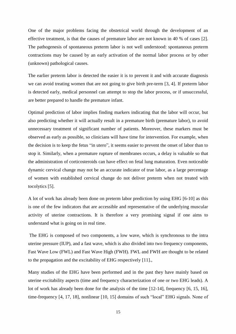
The EHG is composed of two components, a low wave, which is synchronous to the intra

uterine pressure (IUP), and a fast wave, which is also divided into two frequency components,

Fast Wave Low (FWL) and Fast Wave High (FWH). FWL and FWH are thought to be related

to the propagation and the excitability of EHG respectively [11].,

Many studies of the EHG have been performed and in the past they have mainly based on

uterine excitability aspects (time and frequency characterization of one or two EHG leads). A

lot of work has already been done for the analysis of the time [12-14], frequency [6, 15, 16],

time-frequency [4, 17, 18], nonlinear [10, 15] domains of such “local” EHG signals. None of

16

these methods are however not currently used in routine practice due to a high variance of the

results obtained and an insufficient prediction rate.

The EHG signals were proven to be nonlinear similarly to all electrophysiological signals

from human body. Therefore a more investigation of nonlinear methods are needed to respect

the nonlinearity of EHG signals and to add additional information to those obtained by linear

method from EHG signal in order to increase the labor prediction rate.

Fewer and more recent studies have been performed on aspects relating to the origin of

uterine contractions and the propagation of the contractile activity between the different parts

of the uterus. EHG propagation and direction investigation is limited to just a few studies [19-

27]. To our present knowledge, no study has ever been aimed at localizing the actual sources

of uterine EMG as the one we present in this work.

In this thesis we plan to focus also on the dynamics of the electrical activity (direction of

propagation, source localization). Our work is focused on developing and improving the

analysis of EHG excitability, propagation, and source localization. We therefore used signals

from a 4x4 matrix of electrodes to give us a much more complete image of the uterus and its

underlying contractile mechanisms. We tried in this work to improve the performance of

nonlinear and propagation methods, by testing their sensitivity to different pre-processing

steps and signal characteristics like sampling frequency, stationarity, and frequency content…

We also decided to study the direction of the propagation. We finally developed a new way of

analyzing EHG signals by localization of their sources.

This analysis could permit the identification of clinically relevant parameters. Extensive

clinical studies will then be required for understanding the relation between the parameters

derived from the EHG signal and the processes leading to labor.

Our contribution to the field of EHG analysis is structured around four main themes:

monovariate nonlinear analysis, bivariate analysis of propagation and its direction,

implementation of an EHG based source localization tool and the improvement of the rat

experimental protocol developed in our laboratory (Figure 1).

17

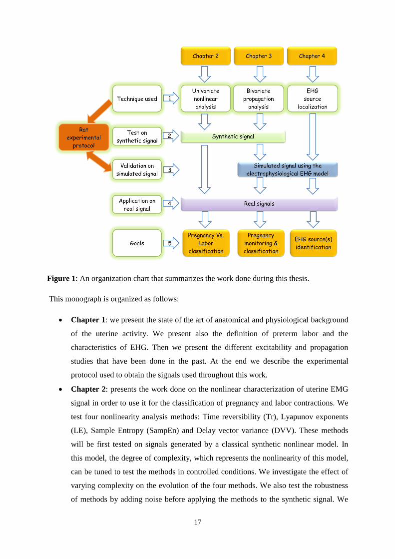
Figure 1: An organization chart that summarizes the work done during this thesis.

This monograph is organized as follows:

Chapter 1: we present the state of the art of anatomical and physiological background

of the uterine activity. We present also the definition of preterm labor and the

characteristics of EHG. Then we present the different excitability and propagation

studies that have been done in the past. At the end we describe the experimental

protocol used to obtain the signals used throughout this work.

Chapter 2: presents the work done on the nonlinear characterization of uterine EMG

signal in order to use it for the classification of pregnancy and labor contractions. We

test four nonlinearity analysis methods: Time reversibility (Tr), Lyapunov exponents

(LE), Sample Entropy (SampEn) and Delay vector variance (DVV). These methods

will be first tested on signals generated by a classical synthetic nonlinear model. In

this model, the degree of complexity, which represents the nonlinearity of this model,

can be tuned to test the methods in controlled conditions. We investigate the effect of

varying complexity on the evolution of the four methods. We also test the robustness

of methods by adding noise before applying the methods to the synthetic signal. We

18

also apply the methods on signals with different SNR values to test which method is

the least sensitive to noise. Surrogate technique is usually used to detect the presence

of nonlinearity in signals. This technique has evidenced the presence of nonlinearity in

EHG signals. The degree of non-linearity can also be estimated by using the z-score

associated with the use of surrogates, but computing is thus time consuming. In our

study we investigate the effect of the use of surrogate on the performances of the

tested methods on synthetic signals, as well as on the classification rate for real

signals. After testing and validating the methods on synthetic signals we apply and

compare them with linear methods on real EHG signals. We will test also at the end of

this chapter the sensitivity of nonlinear methods to the sampling frequency and to the

frequency contents of EHG signals.

Chapter 3: presents the bivariate study. We try here to improve the performances of

coupling detection methods to improve the classification of pregnancy and labor

contractions. The new idea in this chapter is that we study by these methods, not just

the coupling value between signals, but also the direction of the coupling. We start our

study from the hypothesis that the synchronization increases from pregnancy to labor.

Pregnancy contractions are supposed to be inefficient and to remain local (small

propagation) while labor contractions are supposed to propagate to the whole uterus in

a short time (fast propagation). We compare two nonlinear methods, nonlinear

correlation coefficient (h2), general synchronization (H) and one linear method

Granger causality (GC), on synthetic Rössler signals in different conditions.

This kind of synthetic signals permits to better understand the behavior of the methods

under varied conditions. However, they are not very representative of the real signals.

We thus also tested the methods on a more physiological model newly developed in

our laboratory. This model can generate a planar wave propagation and a circular

wave propagation of action potential. We apply in this chapter the methods on signals

simulated by this model, to investigate if they permit to detect the right direction of the

given propagated wave.

The final step in this chapter is to apply the methods, tested and validated by using

synthetic and simulated signals, on real EHG signals. We apply them on pregnancy

and labor groups of real contractions to see the capability of methods in differentiating

between these two groups. To study the evolution of uterine synchronization during

pregnancy, we also apply the methods on 8 groups of signal regrouped in terms of

19

week before labor (WBL) and going from 7 WBL to labor. We proposed to improve

the results by using a filtering-windowing approach.

Chapter 4: in this chapter we tackle the study the EHG source localization, which

requires solving a forward and an inverse problem. Therefore we used the „Fieldtrip‟

free toolbox to implement a tool for EHG source localization. We solve the inverse

forward problem using the boundary element method (BEM) method, and the inverse

problem using the minimum norm estimate (MNE) method. We validate our method

using simulated signals with different source locations, then apply this localization

algorithm to real EHG for the source(s) localization of pregnancy and labor

contractions.

Appendix: we develop a suction electrode matrix for the animal experimentation

protocol. This experimentation will be used to record uterine EHG from rat uterus to

validate the physiological EHG model developed in our team and our methods. The

benefit of using the rat uterus is that it contains two well organized layers of muscle

fibers, structure that is not present in the human uterus: a longitudinal superficial layer

and a deep circular layer of muscle fibers. So validation of the model and methods can

be done easier because of the expected direction of propagation with the rat uterus,

which is not possible with woman‟s uterus.

Discussion and general conclusions of this thesis are given with propositions for

possible future work.

The results obtained in this thesis permitted us to write 3 published journal papers, 2

submitted journal papers, 5 international conference papers, and 1 national conference paper.

List of author’s publications

Journal papers

Ahmad Diab, Mahmoud Hassan, Jérémy Terrien, Sofiane Boudaoud, Catherine Marque, and

Brynjar Karlsson, “Improving Connectivity Measures Performance and Stability in Uterine

EMG analysis,” IEEE Transactions on Biomedical Engineering, 2014. (Submitted).

Publication related to chapter 3.

Ahmad Diab, Mahmoud Hassan, Jérémy Laforet, Asgeir Alexandersson, Brynjar Karlsson,

and Catherine Marque, “Analysis of Connectivity Strength and Direction of Simulated and

20

Real Multielectrode EHG Signals,” Medical & Biological Engineering & Computing, 2014.

(Submitted). Publication related to chapter 3.

Dima Alameddine, Ahmad Diab, Charles Muszynski, Brynjar Karlsson, Mohamad Khalil,

and Catherine Marque, “Selection Algorithm for Parameters to Characterize Uterine EHG

Signals for the Detection of Preterm Labor,” Signal Image and Video Processing, 2014.

Publication related to chapter 2.

Ahmad Diab, Mahmoud Hassan, Catherine Marque, and Brynjar Karlsson, “Performance

analysis of four nonlinearity analysis methods using a model with variable complexity and

application to uterine EMG signals,” Medical Engineering & Physics, vol. 36, no. 6, pp. 761–

767, Jun. 2014. Publication related to chapter 2.

Ahmad Diab, Mahmoud Hassan, Brynjar Karlsson, and Catherine Marque, “Effect of

decimation on the classification rate of non-linear analysis methods applied to uterine EMG

signals,” IRBM, vol. 34, no.4-5, pp. 326–329, Oct. 2013. Publication related to chapter 2.

International conference papers

Ahmad Diab, Mahmoud Hassan, Jeremy Laforet, Brynjar Karlsson, and Catherine Marque,

“EHG Source Localization Using Signals from a Uterus Electrophysiological Model,” in

Proc. Virtual Physiological Human Conference 2014 (VPH), Trondheim, Norway, Sep. 2014.

(Accepted). Publication related to chapter 4.

Catherine Marque, Ahmad Diab, Jérémy Laforêt, Mahmoud Hassan, and Brynjar Karlsson,

“Dynamic behavior of uterine contractions: an approach based on source localization and

multiscale modeling,” in Proc. six international conference on Knowledge and Systems

Engineering (KSE), Hanoi, Vietnam, Oct. 2014. (Accepted). Publication related to chapter 4.

Ahmad Diab, Mahmoud Hassan, Sofiane Boudaoud, Catherine Marque, and Brynjar

Karlsson, “Nonlinear estimation of coupling and directionality between signals: Application

to uterine EMG propagation,” in Proc. IEEE Eng. Med. Biol. Soc. Conf. 2013, Osaka, Japan,

Jul. 2013, pp. 4366-4369. (Poster presentation). Publication related to chapter 3.

Ahmad Diab, Mahmoud Hassan, Jeremy Laforet, B. Karlsson, and C. Marque, “Estimation

of Coupling and Directionality between Signals Applied to Physiological Uterine EMG

Model and Real EHG Signals,” in Proc. XIII Mediterranean Conference on Medical and

21

Biological Engineering and Computing 2013, Sevilla, Spain, Sep. 2013, pp. 718-721. (Oral

Presentation). Publication related to chapter 3.

Ahmad Diab, Mahmoud Hassan, Catherine Marque, and B. Karlsson, “Comparison of

methods for evaluating signal synchronization and direction: Application to uterine EMG

signals,” in 2nd International Conference on Advances in Biomedical Engineering (ICABME)

2013, Tripoli, Lebanon, Sep. 2013, pp. 14-17.(Oral presentation). Publication related to

chapter 3.

Ahmad Diab, Mahmoud Hassan, Catherine Marque, and Brynjar Karlsson, “Quantitative

performance analysis of four methods of evaluating signal nonlinearity: Application to uterine

EMG signals,” in Proc. IEEE Eng. Med. Biol. Soc. Conf. 2012, San Diego, California, Aug.

2012, pp.1045-1048. (Oral Presentation). Publication related to chapter 2.

National conference paper

Ahmad Diab, Mahmoud Hassan, Brynjar Karlsson, and Catherine Marque, “Effect of

decimation on the classification rate of nonlinear analysis methods applied to uterine EMG

signals,” in Proc. Conférence de Recherche en Imagerie et Technologies pour la Santé

(RITS), Bordeaux, France, 2013. (Oral presentation). Publication related to chapter 2.

References




[3] J. M. Denney, J. F. Culhane, and R. L. Goldenberg, “Prevention of preterm birth,” Womens

Health (Lond Engl), vol. 4, pp. 625-38, Nov 2008.



[5] J. Linhart, G. Olson, L. Goodrum, T. Rowe, G. Saade, and G. Hankins, “Pre-term labor at 32 to

34 weeks' gestation: effect of a policy of expectant management on length of gestation,” Am. J.

Obstet. Gynecol., vol. 178, 1998.



22















1993.





2, pp. 149-53, Apr. 2001.


555, pp. 153-175, Apr-May. 1956.
















23






745-61, Jun. 2009.


R. E. Garfield, “Noninvasive uterine electromyography for prediction of preterm delivery,” Am

J Obstet Gynecol, vol. 204, pp. 228 -238, 2011.

[23] E. Mikkelsen, P. Johansen, A. Fuglsang-Frederiksen, and N. Uldbjerg, “Electrohysterography of


Scandinavica, vol. 92, no. 9, pp. 1070-1078, 2013.



pp. e86775, 2014.



Gynecol., vol. 200, no. 1, pp. 54.e1–54.e7, 2009.

[26] H. de Lau, C. Rabotti, R. Bijloo, M.J. Rooijakkers, M. Mischi, and S.G. Oei, “Automated

conduction velocity analysis in the electrohysterogram for prediction of imminent delivery: a

preliminary study,” Computational and Mathematical Methods in Medicine, vol. 2013, 7 pages,

2013.

[27] C. Rabotti, M. Mischi, G.S. Oei, and J.W.M. Bergmans, “Noninvasive Estimation of the

Electrohysterographic Action-Potential Conduction Velocity,” IEEE Trans. on Biomedical

Engineering, vol. 57, no. 9, pp. 2178-2187, 2010.

24

Chapter 1: The uterus, preterm labor and measuring EHG.

1.1 Introduction

The ultimate goal of the work presented in this thesis is the detection of labor and the

prediction of preterm labor, by analyzing the propagation of the uterine electrical activity

(electrohysterogam, EHG) through the uterus, during labor and pregnancy. The uterus is a not

well-understood organ. It is deceptively simple in structure but its behavior, when it goes

from pregnancy towards labor, indicates that there are numbers of interconnected control

systems involved in its functioning (electric, hormonal, mechanical). The physiological

phenomena underlying labor are however still not completely understood.

Uterine contractility can be thought of as being dependent on two aspects, cells excitability

and propagation of electrical activity to a part of, or the whole, uterus. Analyzing these two

aspects as well as the localization of source(s) of uterine activity can bring useful information

for the prediction of preterm labor. A lot of studies have been done on using excitability

characteristic, in order to detect preterm labor [1-6], whereas, until recently, less effort has

focused on characterizing the propagation of electrical activity. Furthermore, no work has

been done concerning the localization of uterine electrical source(s).

In this chapter, we first give background on the physiology of the uterus, then on the factors

that contribute to the generation of uterine contraction and to its propagation. We present then

some of the basic characteristics of the EHG, and the methods that have previously been used

for the detection of preterm labor threat. Finally we describe how EHG is recorded and the

experimental protocol used to acquire the human EHG used throughout this thesis.

1.2 Uterine anatomy and physiology: an overview

1.2.1 Anatomy of the uterus

The non-pregnant uterus is pear-shaped, 7.5 cm in length, 4 to 5 cm in width at its upper

portion, and 2 to 3 cm in thickness, and made up of the fundus, body and cervix (Figure 1.1).

The uterine (Fallopian) tubes enter each superolateral angle, termed the cornu, above which

lies the fundus. The uterine body narrows to a waist (the isthmus), which continues as the

25

cervix. The cervix is gripped around its middle by the vagina, and this attachment defines a

supravaginal and a vaginal part of the cervix [7].

Figure 1.1: Subdivision and layers of the uterus [8].

The uterus is made up of three layers of tissue. The outer serosa layer, the middle muscular

layer called myometrium which makes up the bulky uterine wall, composed of 3 layers of

smooth muscle, and the innermost, composed of specialized mucous membrane,

endometrium. The endometrium contains abundant blood supply. It is composed of two

layers. These are stratum functionalis that shed during every menstruation. If pregnancy

occurs it continues to be site of attachment and nourishment for morrula (fertilized zygote).

The second layer of endometrium is stratum basale that attaches to myometrium [9]. The

myometrium is the middle and thickest layer of the uterus. It is composed of longitudinal and

circular layers of smooth muscle. During pregnancy, the myometrium increases both by

hypertrophy of the existing cells and by multiplication of the cell number. When parturition

takes place, coordinated contractions of the smooth muscle cells in the myometrium occur to

expel the fetus out of the uterus. The serosa or peritoneum is the outermost layer of the uterus.

It is a multilayered membrane that lines the abdominal cavity and supports and covers the

organs.

The smooth cells progressively increase in size during the last stage of gestation with a

maximum length of 300 μm and a maximum width of 10 μm [10]. Contractions of smooth

muscle cells happen due to the interaction of myosin and actin filaments.

26

The uterine smooth muscle fibers are arranged in overlapping tissue-like bands, the exact

arrangement of which is a highly debated topic [11]. All myocytes (uterine muscle cells) are

gathered in packages or "bundles" (Ø 300 + / - 100 microns) with junctions between them.

Packets are contiguous within a bundle or fasciculus. The bundles are arranged parallel to the

surface of the uterus, transversely at the fundus and obliquely downward. Communicating

bridges, named Gap Junctions, connect adjacent bundles. A diagram of this structural

organization is shown Figure 1.2.

Figure 1.2: Three-dimensional structure of the woman uterus [12].

1.2.2 Uterine activity

The mechanical activity of the non-gravid uterus is cyclic and depends on the hormonal

menstrual cycle. It includes an activity phase spread throughout the whole uterus, which

permits the expulsion of blood and debris endometrial. The beginning of the cycle is

characterized by contractions spread to the entire uterus directed towards the cervix and by

frequency equal to 1-3/min. The mid-cycle, ovulatory period, is characterized by strong and

regular contractions directed to the fundus of the uterus, with a frequency equal to 10/min,

and which is thought to promote the progress of sperm. Then a quiescent phase occurs. It

corresponds to the development of the endometrium that is required for any eventual

implantation. The contractions are local, low-intensity directed towards the bottom and of

frequency equal to 265/min [13].

The gravid uterus also contains a phase of relative quiescence during most of the pregnancy

stage, followed by a period of activity leading to childbirth. In women, two types of uterine

activities coexist:

27

- Contractions of very low amplitude, with frequency of 1/min and very local influence,

named Low Amplitude High Frequency (LAHF, Onde Alvarez - OA- in French).

- Contractions of higher amplitude and lower frequency (one every 3 or 4 hours, at the

beginning of their emergence around 18 weeks of gestation). These contractions called

Braxton Hicks contractions become more frequent and stronger when approaching the term (1

per hour at 30th week) and have a wider field of influence than that of LAHF [14-15].

The most significant change noticed in early labor concerns the spread of activity. From

partially propagated in late pregnancy, labor contractions become strong, rhythmic and spread

to the entire uterus in a short time. The insertion of intrauterine catheters (= internal

tocography) allows the recording and the definition of a set of parameters describing uterine

contractions (UC) (Figure 1.3). These parameters are:

- The basic tone.

- The amplitude of UC.

- The frequency of UC.

- The duration of UC.

Figure 1.3: A diagram illustrating the different parameters of the uterine contraction (UC),

edited from [16].

During normal labor, the uterine activity quantified by these different parameters will

gradually increase. The basic tone varies from 5 to 13 mm Hg [17]. The total amplitude of the

UC, which takes into account the basic tone, varies from 30 to 65 mmHg. In practice, the

basal tone is not taken into account and therefore it is the active amplitude (or real intensity)

Interval between 2 UC

Frequency

Active

amplitude

Basal tone

Total

amplitude

Duration

28

of UC which is usually considered [17]. The average interval between 2 UC (period) gives the

frequency of UC in 10 minutes. It is initially 1 to 3 UC / 10 min and reached normally 4 or 5

UC / 10 min at the end of labor. Meanwhile, the average duration of the UC goes from 60 sec

to 85 sec [18].

1.2.3 Cellular and ionic bases of myometrial contraction

In the uterine smooth muscle as in other smooth muscle, calcium seems to be the decisive and

essential element of the intracellular mechanisms underlying the contractile activity. The key

enzyme is the myosin light chains kinase (MLCK) which, activated by the complex Ca2+-

calmoduline (Ca2+

-CaM), phosphorylates the myosin light chain LC20 (Figure 1.4). It is in

this phosphorylated form that myosin can interact with actin and cause contraction. The fall in

the concentration of intracellular calcium [Ca2+

]i leads to relaxation: the dephosphorylated

myosin, by the action of a specific phosphating, then detaches from the actin. Furthermore,

phosphorylation of MLCK causes a decrease in its ability to activate myosin and thereby to

produce the contraction. This activation pattern (related to depolarization followed by

repolarization) is well established in vitro but does not always seem to be strictly followed in

vivo. In addition, the relative importance of different control channels varies according to

whether it is a spontaneous contractile activity or that caused by extracellular signals. Some

animal studies suggest the existence of other regulatory pathways involving protein kinase C

(PKC) and the fine filament proteins, the caldesmon and calponin, whose role is far from

being elucidated in the uterus [19-20].

Figure 1.4: Biochemical mechanism of contraction (_____) and relaxation (- - - -) of the

uterine muscle. MLCK: Kinase of myosin light chains [20].

29

Different structures and mechanisms are responsible for the increase in the concentration of

free Ca, [Ca2+

]i, from about 10-7

to 10-6

M, which is essential for the activation of MLCK.

Calcium channel conductance can be activated by a change in transmembrane potential

(VOC-Voltage operated channels), of type L ("long lasting") and T ("transient"), by fixing a

specific ligand (ROC, Receptor-operated channels) or by mechanical constraint. The available

[Ca2+

]i can also come from intracellular sites which have an increasing capacity for storing

Ca2+

as gestation progresses.

1.2.4 Propagation of the uterine activity

The cause of uterine contractility is mainly myogenic. The muscle is solely responsible for its

contraction, although intrinsic (mechano-receptor ...) and extrinsic control (sympathetic and

parasympathetic systems) is present. Close to the time of delivery, the uterus initiates and

coordinates the firing of individual myometrial cells to produce organized contractions

causing the expulsion of the fetus from the mother‟s body. The contractile activity of the

uterus results from the excitation and propagation of electrical activity.

Myometrial cells are coupled together electrically by gap junctions composed of connexin

proteins [21]. This grouping of connexins provides channels of low electrical resistance

between cells, and thereby furnishes pathways for the efficient conduction of action

potentials. Throughout most of pregnancy, and in all species studied, these cell-to-cell

channels or contacts are low, with poor coupling and decreased electrical conductance, a

condition favoring quiescence of the muscle and the maintenance of pregnancy. At term,

however, the cell junctions increase and form an electrical syncytium required for

coordination of myometrial cells for effective contractions. The presence of the contacts

seems to be controlled by changing estrogen and progesterone levels in the uterus [21]. The

Gap Junction bridges are responsible for conducting the rapid communication of the action

potential between different bundles [12].

Another mechanism for controlling the uterine activity is through calcium waves [22].

However, it is necessary to distinguish two types of wave: the intracellular calcium wave and

the intercellular calcium wave. The intracellular calcium wave is consistent with rapid

changes in intracellular calcium concentration [Ca2 +] in a single cell. This wave is capable of

crossing the cell membrane and becomes an intercellular calcium wave. The intercellular

calcium wave propagates slowly (~ 4 microns / sec) and to a relatively low maximum distance

(~300 microns) corresponding to the size of a bundle [22-23].

30

Like cardiac cells, uterine myometrial cells can generate either their own impulses -

pacemaker cells- or can be excited by the action potentials propagated from the other

neighboring cells -pacefollower cells. But unlike cardiac cells, each myometrial cell can

alternately act as a pacemaker or a pacefollower. In other words, there is no evidence of the

existence of a fixed anatomic pacemaker area on the uterine muscle [11, 24]. The spontaneous

oscillations in the membrane potential of the autonomously active pacemaker cells lead to the

generation of an action potential burst when the threshold of firing is reached. The electrical

activity arising from these pacemaker cells excites the neighboring cells, because they are

coupled by electronic connections called gap junctions. It is believed that the action potential

burst can originate from any uterine cell, thus the pacemaker site can shift from one

contraction to another [11, 24].

Many hypotheses on the pacemaker cells have been issued including their number, position ...

It seems that there is a one or more preferential pacemaker activities loci near the fundus, as

found by Caldeyro-Barcia et al. [25]. This activity is then propagated in all directions, but

ultimately from the fundus to the cervix.

1.3 Uterine electromyography

Uterine electrical activity is the result of the depolarization and repolarization of thousands of

myometrial smooth muscle cells [10-11, 24]. The immediate succession of depolarization and

repolarization phases of a myometrial cell induces a burst of action potentials. It has been

shown that each contraction is associated to a burst of action potentials. The uterine

electromyogram arises from the generation and transmission of these bursts of action

potentials in the uterine muscle. By spreading through gap junctions, from one myometrial

cell to another, this activation results in an increased and organized electrical activity,

particularly in the last trimester of pregnancy and during labor [26]. This increased, organized

uterine electrical activity precedes the uterine mechanical contraction and is associated to

cervical shortening and dilatation, a phenomenon known as the uterocervical reflex [11, 27-

29]. The frequency of the action potential within a burst, the duration of the burst and the total

number of simultaneously active cells are directly related to the frequency, duration and

amplitude of a contraction.

Early studies of the uterine electromyographic signal were performed by internal

electromyography. They allowed the detailed description of the EMG signal, during

31

contraction, as an electrical activity whose frequency is mostly between 0.1 and 1Hz and that

has an amplitude between 100 μV and 1.8 mV [30]. Simultaneous recording of internal and

external EMG activity on the same woman showed a very good correlation between the two

signals [11, 31]. This demonstrated that the surface EMG signal is representative of the

electrical activity of the uterine muscle. These results have been confirmed in an analysis of

the EMG signal of the pregnant macaque [4]. Using these results, the external uterine EMG

has become a standard non-invasive method for the study of uterus electrical activity.

The electrohysterogram (EHG), that is the uterine EMG recorded, by using surface electrodes,

is characterized by a low frequency activity (0.1 to 0.3 Hz) with a superimposed activity of

higher frequency (FW, fast Wave: 0.3 to 2 Hz). The low frequency signal is considered as the

result of mechanical disturbances induced by the deformation of the abdomen under the effect

of contractions [32]. At the opposite, FW (parted then in two components FWL - Fast Wave

Low- and FWH - Fast Wave High) is related to uterine contractions. A comparison study

between contractions during pregnancy and labor showed that, for both type of contractions,

the EHG energy is predominantly in the 0.2 - 3 Hz frequency band [2]. It has also been shown

that there is nevertheless a difference in frequency distribution between these two types of

contraction (pregnancy and labor). A shift towards higher frequencies is observed as term

progresses [2].

Propagation of the uterine electrical activity

Electromyography studies performed by Garfield et al. show that there is infrequent and

unsynchronized low uterine electrical activity throughout most of the pregnancy [33-34]. This

is also demonstrated in the recording of human uterine electrical events (EHG) acquired from

the abdominal surface during pregnancy [11]. There is little uterine electrical activity,

consisting of infrequent and low amplitude EMG bursts, throughout most of pregnancy. When

bursts occur prior to the onset of labor, they often correspond to periods of perceived

contractility by the patient. During term and during preterm labor, bursts of EMG activity are

frequent, of large amplitude, and are correlated with the large changes in intrauterine pressure

and pain sensation.

The increase in gap junction number, and the resulting facilitated electrical transmission,

provide better coupling between the cells resulting in synchronization and coordination of the

contractile events of the whole uterus.

32

Thus the efficiency of contractions leading to labor depends on the burst activity synchronized

over a large area of the uterus [35]. Therefore it is important to determine the extent of

propagation throughout the multi-cellular uterine muscle bundle. Since the propagation of

these uterine contractions can be in both longitudinal and transverse direction, due to the

complex uterine structure, we need to determine the propagation characteristics over the entire

maternal abdomen while performing surface recordings. We believe that information

regarding the spatial-temporal activation of the uterus may be predictive of onset of labor

leading to the delivery of the fetus. Thus, a complete spatial-temporal mapping of uterine

activity throughout pregnancy is a key parameter that will improve the understanding of the

uterine contraction mechanism.

1.4 Premature labor

According to the definition of the World Health Organization (WHO), preterm delivery is a

delivery at a gestational age of less than 37 completed weeks or less than 259 days of

amenorrhea. Every birth occurring after 22 weeks of amenorrhea and before 37 weeks is

defined as a premature birth. A birth occurring before 22 weeks of amenorrhea is considered

as an abortion by WHO.

Preterm labor is a topical issue because out of 750,000 births in France, 44,000 are premature

[36]. Preterm labor is still the most common obstetrical complication during pregnancy, with

20% of all pregnant women at high risk of preterm labor. In the United States, more than half

a million babies -that's 1 of 8- are born premature each year. At 1500 $ a day for neonatal

intensive care, this constitutes expenditure well over 4 billion $ each year. Also, preterm birth

accounts for 85% of infant mortality and 50% of infant neurologic disorders [37].

Preterm birth is a pathology that can lead to serious consequences for the child and has also a

socio- economic cost. The main risks to children are:

• Respiratory distress (often associated with hyaline membrane disease)

• Infection

• Neurological Diseases

• Hypothermia

• Necrotizing enterocolitis

33

Over the last 20 years, advances in neonatal care for children of less than 1500 grams have

increased significantly their survival rate. One of the major problems facing the obstetrical

world through the development of an effective treatment, is that the causes of premature labor

are not known in 40 % of cases [38]. However, some factors appear to play an important role

in the prevention of preterm labor.

Socio-economic factors, microbial infections, uterine anomalies, premature rupture of

membranes and various pathologies of pregnancy are factors involved in the risk of preterm

labor.

The preterm birth rate has changed little over the past 30 years. Only France [39], Finland and

Norway [40] observed a decrease between the late 60s and 80s. In France, the prematurity rate

has stabilized between 1990 and 1995; it was 5.4% in 1995 [41]. Live births before 37 weeks

increased steadily from 5.4% in 1995 to 6.6% in 2010 [42]. It reached 7 % in Canada and

more than 10% in the United States [43] at the same time.

1.4.1 Detection of labor and prediction of premature labor

Optimal detection of labor implies finding markers indicating that the labor will occur, but

also predicting whether it will actually result in a premature birth (premature labor), to avoid

unnecessary treatment of significant number of patients. Moreover, these markers must be

observed as early as possible, so clinicians will have time for intervention. For example, when

the decision is to keep the fetus “in utero”, it seems easier to prevent the onset of labor than to

stop it. Similarly, when a premature rupture of membranes occurs, a delay is valuable so that

the administration of corticosteroids can have effect on fetal lung maturation.

There are several methods presently used for the detection of preterm delivery among them:

- Measurement of biochemical markers:

• Fetal Fibronectin (FFN) [44].

• α-fetoprotein [45].

• Placental peptides [46].

They have been proposed as methods for monitoring patients that have a risk for premature

labor. Some results show that FFN can be used for the prediction of premature labor [47]

although with poor likelihood ratios.

- Clinical diagnosis: This technique includes cervical dilation and effacement, vaginal

bleeding, or ruptured membranes [48].

34

- Maximal uterine contractions: This technique measures the maximal number of contraction

events seen in any 10-min period, measure done by a clinician based on tocodynamometer

(TOCO) [49]. Tocodynamometers (TOCO) are external devices aiming to measure the force

generated by the slight movement of the uterus caused by uterine contractions measured on

the mother‟s abdomen. They give an indirect indication of uterine contraction. Their non-

invasiveness allows the devices to be used for all pregnancies without risk to the fetus or to

the mother. They are used in nearly all births in a medicalized setting. Nevertheless, TOCO

monitoring is uncomfortable, inaccurate and depends on the subjective interpretation of the

examiner. Intrauterine pressure (IUP) catheters provide the best information concerning

uterine contractions, allowing the exact quantification of the mechanical effect of

contractions. But the clinical usefulness of this technique is limited by its invasiveness, since

it requires prior rupture of membranes in order to insert the pressure device into the uterus.

This can increase the risk of infection or accidental induction of labor [50].

- Abdominal and transvaginal ultrasound: No clear success was achieved by using this

technique to detect premature labor [51]. However, this technique gives prediction later after

the onset of preterm labor symptoms. Furthermore, the measurement of the cervical length by

ultrasonography is largely influenced by the varying amounts of urine in the bladder [47].

- Detection of the circadian rhythm of uterine activity [52].

Most of these methods of evaluation and monitoring of premature labor suffers from a

problem of sensitivity and objectivity. Current treatment methods are however most effective

when the detection of labor is made early. They are not usually applied unless the threat of

labor is certain.

Other directions have been more recently investigated in order to define a reliable marker of

preterm labor threat:

- Magnetomyography (MMG): This technique measures noninvasively the magnetic fields

associated with the uterine action potentials. Eswaran et al did the first MMG recordings of

spontaneous uterine activity by using 151 magnetic sensor array [53].

- Uterine electromyography or Electrohysterogram (EHG): Uterine EMG is the result of

electrical activity originating from the depolarization-repolarization of billions of smooth

muscle myometrial cells. It has been proved that synchronous myometrial and abdominal

activities occur, which are temporally correlated with the mechanical activity of the uterus

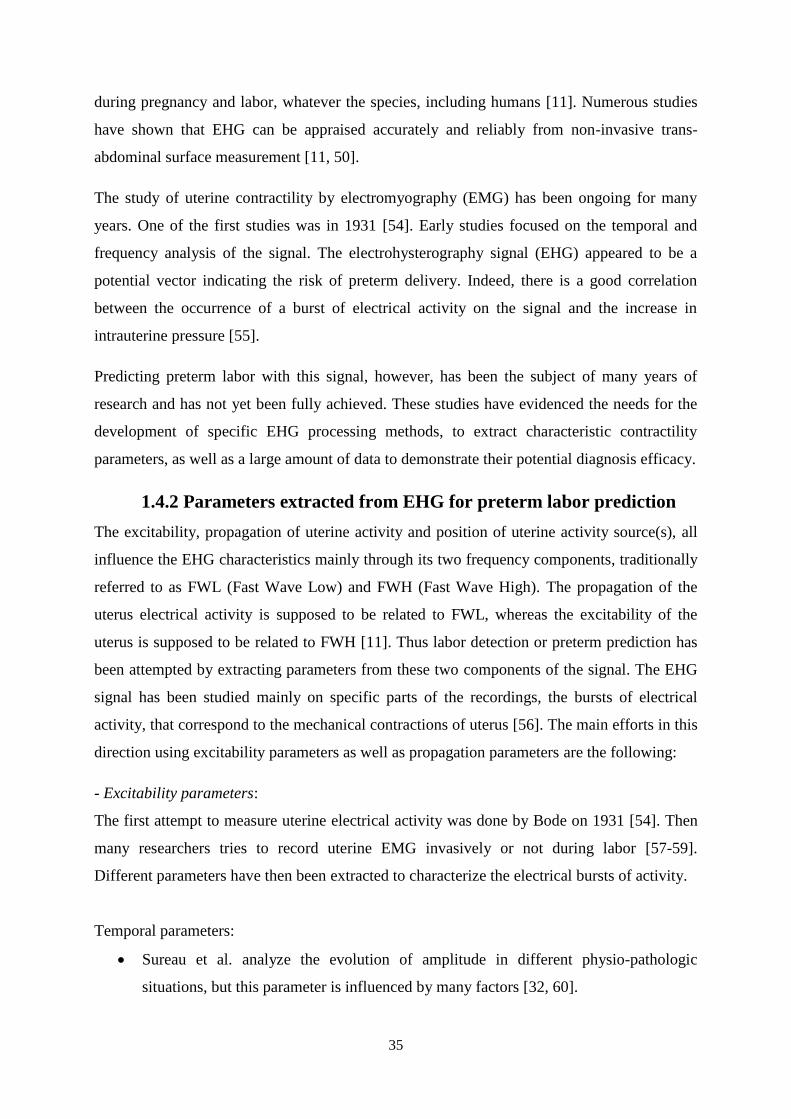
35

during pregnancy and labor, whatever the species, including humans [11]. Numerous studies

have shown that EHG can be appraised accurately and reliably from non-invasive trans-

abdominal surface measurement [11, 50].

The study of uterine contractility by electromyography (EMG) has been ongoing for many

years. One of the first studies was in 1931 [54]. Early studies focused on the temporal and

frequency analysis of the signal. The electrohysterography signal (EHG) appeared to be a

potential vector indicating the risk of preterm delivery. Indeed, there is a good correlation

between the occurrence of a burst of electrical activity on the signal and the increase in

intrauterine pressure [55].

Predicting preterm labor with this signal, however, has been the subject of many years of

research and has not yet been fully achieved. These studies have evidenced the needs for the

development of specific EHG processing methods, to extract characteristic contractility

parameters, as well as a large amount of data to demonstrate their potential diagnosis efficacy.

1.4.2 Parameters extracted from EHG for preterm labor prediction

The excitability, propagation of uterine activity and position of uterine activity source(s), all

influence the EHG characteristics mainly through its two frequency components, traditionally

referred to as FWL (Fast Wave Low) and FWH (Fast Wave High). The propagation of the

uterus electrical activity is supposed to be related to FWL, whereas the excitability of the

uterus is supposed to be related to FWH [11]. Thus labor detection or preterm prediction has

been attempted by extracting parameters from these two components of the signal. The EHG

signal has been studied mainly on specific parts of the recordings, the bursts of electrical

activity, that correspond to the mechanical contractions of uterus [56]. The main efforts in this

direction using excitability parameters as well as propagation parameters are the following:

- Excitability parameters:

The first attempt to measure uterine electrical activity was done by Bode on 1931 [54]. Then

many researchers tries to record uterine EMG invasively or not during labor [57-59].

Different parameters have then been extracted to characterize the electrical bursts of activity.

Temporal parameters:

Sureau et al. analyze the evolution of amplitude in different physio-pathologic

situations, but this parameter is influenced by many factors [32, 60].

36

Gondry et al. follow of uterine activity during pregnancy “longitudinal study” using

EHG temporal characteristic [61].

Root mean square (RMS) value was used to detect the risk for preterm delivery [62].

Spectral parameters:

When authors began the investigation the uterine EMG frequency content, they were

limited at the begin to the slow wave band [59, 63]. But they doubted that the slow

wave had any physiological meaning.

Therefore most authors then studied only the electrohysterogram in the frequency

band corresponding to FWH. They soon found a synchronization between the

abdominal and myometrial electromyogram activities [28, 30, 64].

The amplitude distribution as well as the power density spectrum median and modus

spectrum of uterine EHG activity bursts were calculated and analyzed [2, 65].

Marque et al. follow the EHG spectral content in function of contraction efficiency

during labor [2].

It was proved that, during pregnancy, uterine activity is minimal and characterized by

electromyographic bursts infrequent, of low amplitude and low frequency content

[61]. This activity becomes frequent, of large amplitude and higher frequency content

during term and preterm labor [2], [27].

It was observed by Marque et al. that the relative energy in the low frequency band to

total frequency band (L/T) decrease whereas the relative energy in the high frequency

band to total frequency band (H/T) increases, creating thus a shift to higher

frequencies as delivery approaches [2].

Close to delivery, the administration of nifedipine, make a shift of modus frequency of

EHG power spectral density to lower frequencies when it is expected to rise [66].

It was shown by Fele-Žorž et al. that the value of median frequency increases with the

approaching of labor, which may be associated with term delivery [67].

The duration, the mean value and/or standard deviation and the modus frequency of

PSD, and the number of bursts per unit time extracted from EHG bursts were also

evaluated. The artificial neural networks classified correctly the majority of term and

preterm laboring and non-laboring bursts using these extracted parameters [68].

Time-frequency parameters:

37

Leman et al. [69-70] used wavelet decomposition to denoise the EHG.

Recently, wavelet transform approaches were used for the prediction of preterm labor

risk [71].

Wavelet analysis was used also for the detection and classification of EHG signals

[72-73].

Marque et al. guide a study for denoising, characterization and classification of EHG

signals using time frequency parameter in order to build a portable device for home

pregnancy monitoring [74].

Duchêne et al. track the instantaneous frequency of the EMG burst recorded internally

on monkey uterus and confirmed the relationship between surface electromyogram

and internal electrical activity at the uterine muscle level [75].

Nonlinear parameters:

Oczeretko et al. showed that the uterine activity of non-pregnant uterus presents

nonlinear features [76]. Nonlinear time series analysis techniques were applied to

uterine EMG signals since they can give information about the nonlinear features of

EHG signals, which arise from the underlying uterus physiological processes [77].

Some researchers claimed to show that the sample entropy method is a promising

method in preterm and term labors classification [67]. They showed also that we can

evaluate the progress of the labor using sample entropy method [78].

Maner et al. showed that the bursts of patients who will deliver spontaneously within

24 h and those who will not can successfully be separated by this wavelet

decomposition generated fractal dimension [79].

Sabry-Rizk et al. examined the nonlinear dynamics of the uterus EMG signals on

normal and abnormal labor contractions in the first stage of the labor. An attractor

structure has been calculated on abdominal EMG signals at various relaxation and

contraction periods. The observed black inertness of attractors was called nucleus.

Precisely, by studying its fractal behavior it was shown that the size of the nucleus

increases with cervical dilatation until it takes over the entire phase-space. The weak

labor contractions, typical for failure in progress in the first stage of labor, showed

predominantly periodic structures with or without small-size nuclei [80].

Recently, time reversibility appear as a useful method for the detection of uterine

EMG nonlinearity characteristic and pregnancy/labor classification [6].

38

But all the nonlinear methods do not have the same performance, as it was shown with

maximal Lyapunov exponent and correlation dimension, that did not manage to

differentiate between labor and non-labor classes [67].

- Propagation parameters:

All the excitability parameters cited above were computed with a monovariate approach (one

burst processed at a time, extracted from a single EHG signal). They, more or less, permited a

differentiation between pregnancy and labor contractions, to provide information for preterm

labor (PTL) diagnosis. As uterine contraction efficiency is related to both excitability and

propagation, the computation of propagation parameters with the excitability one might

improve this classification. Only few studies have been done to characterize the propagation

of EHG signal. These studies can be summarized as following:

Linear and nonlinear correlation:

Marque et al. have observed more correlation in low frequencies than high frequencies

using the linear correlation coefficient which support the hypothesis that the

propagation is related to FWL [81].

Duchêne et al. were interrested in stuying uterine EMG propagation using

autocorrelation, cepstrum and deconvolution function [82].

The linear inter-correlation remains the main method that has been used for EHG

propagation analysis [82-83].

The inter-correlation function was used also by Mansour et al. to analyze the

propagation of the internal uterine EMG on four internal electrodes, sutured on the

uterus of a monkey during labor [4]. The signals were first filtered into FWL and

FWH frequency bands. Then the inter-correlation function was calculated for each

wave between the two pairs of electrodes. The results coincide with the hypothesis

that the correlation is always higher for FWL than for FWH.

Most of the researchers said that the synchronization of uterine electrical activity is the

most important factor that leads to an efficient labor. To analyze the synchronization,

uterine EMG activity can be recorded from the abdominal surface using multi-

electrode measuring systems. Jiang et al. simultaneously measured uterine EMG

activity using 16 channels [84]. They obtained 297 contractions from twenty patients

39

in labor. The energy on the frequency range between 0.2 and 0.45 Hz (FWL) and

between 0.8 and 3 Hz (FWH) was calculated. In this study, analysis was restricted to

the relative energy (H/L) of uterine EMG signals. The energy was computed for each

channel individually, and divided by the minimum of the 16 channels. Then they

imaged the synchronization of uterine contractions by means of uterine EMG

topography. This method of representing the synchronization uses the relative

amplitudes of uterine EMG signals in relation to the surface of uterus.

It was proposed that the prediction of labor may be increased by the observation of

synchronization together with the classical time – frequency analysis [85].

Recently, it has been shown that the nonlinear correlation between EHG signals

increases from pregnancy to labor [86]. However, in this study, authors have analyzed

the connectivity on the whole uterine bursts (no pre-segmentation).

The segmentation of monkey uterine EHG signals using bivariate and univariate

piecewise stationary pre-segmentation algorithm was done successfully by Terrien et

al. [87-88] and a comparison between univariate and bivariate segmentation algorithm

was done. They investigate in this study the effect of taking only the higher frequency

component of signal on the behavior of the nonlinear correlation within the EHG

burst.

The investigation of the effect of filtering human uterine EHG signals within its

different frequency component (low and high component) was done also by Terrien et

al. [89]. They prove that filtering the signals within FWL which is supposed to be

related to propagation of EHG signals, increases the pregnancy/labor classification

rate using nonlinear correlation coefficient method and makes the difference between

both group more significant.

Identification of uterine activity origine, its movement and velocity:

Planes et al. begin the quantification of propagation velocity using linear correlation

[90].

Using 240 extracellular electrodes placed around the whole uterus, Lammers et al.

[91] measure the electrical activity of the term pregnant guinea pig uterus. Using this

recording, they calculate the velocity of longitudinal and circumferential conduction.

40

Thus, they study the two-dimensional spread and the propagation of signals. They

found that the velocity of spikes propagation is about 7 cm/s in the longitudinal

direction, where the muscle bundles lie parallel to the plane of propagation, and about

3 cm/s in the circular direction, where muscle is organized at right angles.

Some authors tried to identify the center of uterine activity by using eight channel

measuring system and calculating continuously the “frequencies of movement

patterns” from normalized and filtered signals. Euliano et. al. [92] followed the

direction of propagation and movement of the center of activity (the origin of the

contraction). This study reports an interesting pattern in women who delivered

successfully: the direction of the center of uterine activity was predominantly to the

fundal. This means that the relaxation of uterus begins from the lower uterine segment

toward the upper portion of the uterus in women who deliver vaginally [92].

Cadeyro-Barcia et al. also claimed by clinical studies that the uterus begins to contract

in the upper fundal region and then this contraction is conducted toward cervix [93].

Lammers et al. [91] conduct a study on the guinea pig uterus that shows that there are

two possibilities for the origin of electrical activity, either the ovarian or cervical end

of the uterus, and that the velocity was not affected by the propagation in either

direction (i.e., toward the ovary or toward the cervix). However, the authors assumed

that activity was initiated mostly in the ovarian end (corresponding to fundus in

humans).

Duchene et al. also show the existence of a constant chronogram during labor by

studying the correlation of EHG envelopes recorded at several sites in the uterus of

delivering macaques [82].

The inter-electrode delay was estimated for surface multichannel EHG recordings in

order to analyze the uterine activity propagation [94]. Authors focused on localizing

pacemaker zones. Localization on the upper part was been observed on 65% of case.

Most of the previous study performed on EHG did not study the directionality between

signals. Whereas, few other studies evidenced a propagation that spreads in all

directions, with a dominant direction down towards the cervix [95-96].

Source localization:

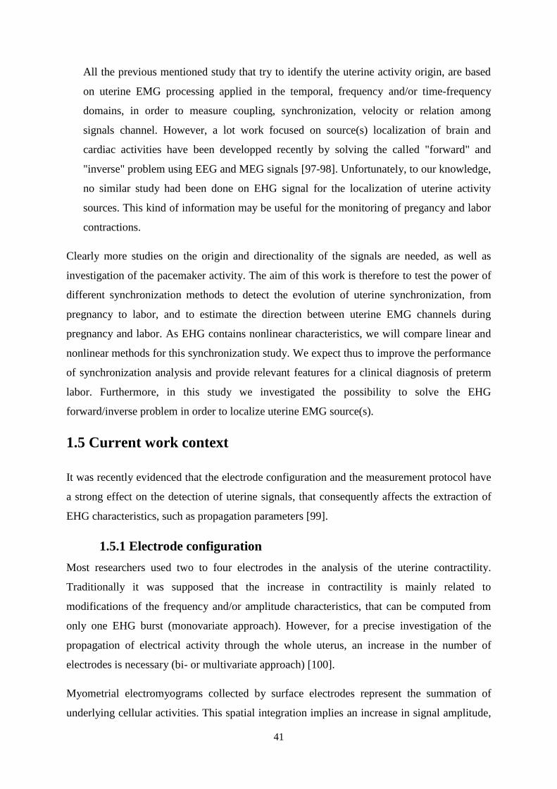
41

All the previous mentioned study that try to identify the uterine activity origin, are based

on uterine EMG processing applied in the temporal, frequency and/or time-frequency

domains, in order to measure coupling, synchronization, velocity or relation among

signals channel. However, a lot work focused on source(s) localization of brain and

cardiac activities have been developped recently by solving the called "forward" and

"inverse" problem using EEG and MEG signals [97-98]. Unfortunately, to our knowledge,

no similar study had been done on EHG signal for the localization of uterine activity

sources. This kind of information may be useful for the monitoring of pregancy and labor

contractions.

Clearly more studies on the origin and directionality of the signals are needed, as well as

investigation of the pacemaker activity. The aim of this work is therefore to test the power of

different synchronization methods to detect the evolution of uterine synchronization, from

pregnancy to labor, and to estimate the direction between uterine EMG channels during

pregnancy and labor. As EHG contains nonlinear characteristics, we will compare linear and

nonlinear methods for this synchronization study. We expect thus to improve the performance

of synchronization analysis and provide relevant features for a clinical diagnosis of preterm

labor. Furthermore, in this study we investigated the possibility to solve the EHG

forward/inverse problem in order to localize uterine EMG source(s).

1.5 Current work context

It was recently evidenced that the electrode configuration and the measurement protocol have

a strong effect on the detection of uterine signals, that consequently affects the extraction of

EHG characteristics, such as propagation parameters [99].

1.5.1 Electrode configuration

Most researchers used two to four electrodes in the analysis of the uterine contractility.

Traditionally it was supposed that the increase in contractility is mainly related to

modifications of the frequency and/or amplitude characteristics, that can be computed from

only one EHG burst (monovariate approach). However, for a precise investigation of the

propagation of electrical activity through the whole uterus, an increase in the number of

electrodes is necessary (bi- or multivariate approach) [100].

Myometrial electromyograms collected by surface electrodes represent the summation of

underlying cellular activities. This spatial integration implies an increase in signal amplitude,

42

and is usually associated with a low pass filtering effect that has been extensively investigated

and modeled in striated muscles [101]. Abdominal electromyograms exhibit the activities

similar to internal electromyograms, except that they are low-pass filtered by the conductive

properties of tissues lying between the uterus and the electrodes [31].

Abdominal electrodes can be located anywhere as long as they are above the corpus uteri.

However, placement along the vertical median axis provides a better signal/noise ratio

because of a closer contact and a more constant position of the uterus relative to the

abdominal wall during contractions [11].

For electrode configuration, most authors choose to record both myometrial and abdominal

electromyograms with bipolar electrodes. So far only Mansour et al. [102] have obtained

noiseless myometrial electromyograms, with monopolar electrodes directly sutured on

monkey uterus. However, for abdominal recordings it is imperative to use bipolar electrodes,

because the signal/noise ratio is lower than for internal ones. Bipolar electrodes reflect the

difference between the two signals present below the two electrodes. Common noise, such as

maternal electrocardiogram, maternal movements, electrode movements, and power line

interference are thus efficiently rejected.

The bipolar recording mode affects the electrohysterogram spectral content. With the usual

model of action potential propagating with a constant speed along a striated muscle fiber,

power spectral density of electromyograms has been shown to depend on the inter-electrode

distance, on the propagation velocity, and on the frequency band of the action potential [103].

Bipolar recording induces a high-pass filtering effect, thus eliminating the very low

frequencies; there is also an increase in the higher frequencies when the distance between

electrodes is small when compared with the distance between the fiber and the recording

electrode pair [101, 103]. Also bipolarization induces a bias to the direction of propagation of

uterine EMG signals by forcing the direction to be horizontal or vertical when the

bipolarization is done between vertical or horizontal electrode pairs respectively.

As a consequence, the monitoring of human uterine activity should only be performed with

bipolar abdominal electrodes, even though the bipolar recording mode induces a high-pass

filtering of the signals. Abdominal electrohysterograms contain information related to

myometrial electromyograms, except that the abdominal signal is low-pass filtered because of

tissue filtering. Otherwise, a complete temporal and spectral electromyogram characterization

43

requires monopolar myometrial EMG recordings, which is obviously not possible for clinical

monitoring.

Recently, attempts have been made for filtering monopolar EHG signals to obtain a proper

signal to noise ratio, suitable for signal processing. To this end, Hassan et al. [104] developed

a powerful EHG filtering methods based on the combination of canonical component analysis

(CCA) and empirical mode decomposition (EMD). He proved that this method, named CCA-

EMD, increases the signals to noise ratio of the monopolar EHG signals. The obtained SNR is

larger than with bipolar EHG and with monopolar EHG filtered by other methods, such as

wavelets and independent component analysis (ICA).

As the bipolarization decreases the spatial resolution, and may also cause a bias for the

correlation analysis, if common electrodes are used to generate adjacent bipolar leads, the use

of monopolar EHG could be of great interest for the study of uterine synchronization.

1.5.2 Multichannel experimental EHG recording protocol

Multichannel EHG signals is usually obtained by using multiple electrodes placed on the

mother‟s abdomen. A high spatial resolution is needed in order to obtain a precise maping of

uterine EHG contractions. The total number of electrodes is however limited by the

abdominal surface, specially when the electrodes should be put along or as near a possible to

the median vertical axis, in order to get a better signal-noise ratio (SNR). The use of

monopolar recordings (signals used independantly) improves spatial resolution and also

prevents from the propagation direction bias induced by the bipolarization of signals (signals

used pairwise).

In order to study the propagation of the uterine electrical activity in the view of predicting

preterm labor, [83] we decided to map uterine electrical activity by placing electrodes in a

four by four grid on the woman‟s abdomen. Indeed we believe that using a grid of 16

electrodes, instead of a smaller number, may help to better understand the underlying

mechanism of uterine contractions as well as to improve the prediction values for preterm

labor.

Placing a large number of electrodes for measurements is time consuming and is difficult to

perform, especially in a labor room setting. For this reason a project was launched in Iceland

in 2009 to design a placement system that decreases placement time, reduces the complexity

of the electrode positioning method, by defining a „standard‟ position for recording. The new

44

design retained involves a guide with holes, guiding the placement, as well as adhesion of the

electrodes by means of a double-coated adhesive sheet. A simple frame ensures correct

positioning of the guide onto the adhesive sheet, while positioning the electrodes. With about

2 cm inter-electrode distance, the 16 electrodes (8mm in diameter) are arranged in a 4x4

matrix. This system permitted us to standardize the signals acquisition during this French-

Icelandic EHG propagation analysis project. A typical example of the matrix placement is

illustrated in Figure 1.5.

Figure 1.5: Typical example of the 4x4 electrodes matrix and TOCO sensor positioned on the

woman‟s abdomen.

The measurements were first performed by using a 16-channel multi-purpose physiological

signal recorder, most commonly used for investigating sleep disorders (Embla A10). We later

used another multi-purpose physiological signal recorder (Porti 32, TMSi) with 32 possible

channels. We used Reusable Ag/AgCl electrodes (8mm diameter). The measurements used in

this work were first performed at the Landspitali University hospital in Iceland, following a

protocol approved by the relevant ethical committee (VSN 02-0006-V2), and then at the

Center of Amiens for Obstetrics and Gynecology in France, following a protocol approved by

the regional ethical committee (ID-RCB 2011-A00500-41) of Amiens Hospital. The subjects

were healthy women either in the first stages of labor having uneventful singleton pregnancies

(Labor population), or healthy women having normal (Landspitali University hospital) or risk

(CGO Amiens) pregnancies at varying gestational age (Pregnancy population). After

obtaining mother‟s informed consent, her skin was carefully prepared using an abrasive paste

and alcoholic solution. After that, the sixteen electrodes were placed on the abdominal wall

according to Figure 1.5. The third electrode column was always put on the uterine median

TOCO

sensor(freque

ncy)

EHG sensor

matrix

Reference

electrode

45

vertical axis and the 10-11th

electrode pair on the middle of the uterus (half way between the

fundus and the symphysis). Two reference electrodes were placed on each of the woman‟s hip

as shown in Figure 1.5.

The signal sampling rate was 200 Hz. The recording device has an anti-aliasing filter with a

high cut-off frequency of 100 Hz. The tocodynamometer paper trace was digitalized in order

to facilitate the segmentation of the uterine contractions.

1.5.3 Thesis roadmap

Monopolar EHG signals are very noisy and have low Signal to Noise Ratio (SNR). Indeed,

they are often corrupted by electronic and electromagnetic noises, as well as by movement

artifacts, skeletal EMG and electrocardiogram from both the mother and the fetus, preventing

their direct use for propagation analysis. This is why, until now, most people studied only

bipolar EHG.

Due to these observation and to the evolution of our team work, this thesis has been divided

in two parts:

- The first step was to gather into one single dataset all the bipolar signals recorded by our

colleagues using the protocol described above. We first processed bipolar signals, in order to

get a correct SNR: vertical bipolar signals (BP1,... BP12) were computed as shown in Figure

1.6. These signals were used when analyzing the nonlinear characteristics of the EHG signal

(chapter 2) since for this study (univariate analysis), we were neither interested in spatial

resolution nor in propagation direction. I processed signals recorded on 23 women in Iceland:

11 recorded during pregnancy (33-39 weeks of gestation) and 12 during labor (39-42 weeks

of gestation); and on 27 women in France: 25 recorded during pregnancy (33-39 weeks of

gestation) and 2 during labor (39-42 weeks of gestation). After segmentation we obtained

from this whole database 115 labor EHG bursts and 174 pregnancy EHG bursts related to

different contractions, for each of the 12 bipolar channels.

- For the bivariate analysis, propagation analysis (synchronization, direction), and for source

localization analysis, the CCA-EMD method was already well established in our team for

denoising the monopolar EHG. As the spatial resolution is very important for propagation

analysis, we there used monopolar signals. Another set was recorded in Iceland by using the

same equipements and by the same operator. We thus used monopolar signals recorded only

in Iceland, in order to get a very homogeneous poulation, made only from normal pregnacy

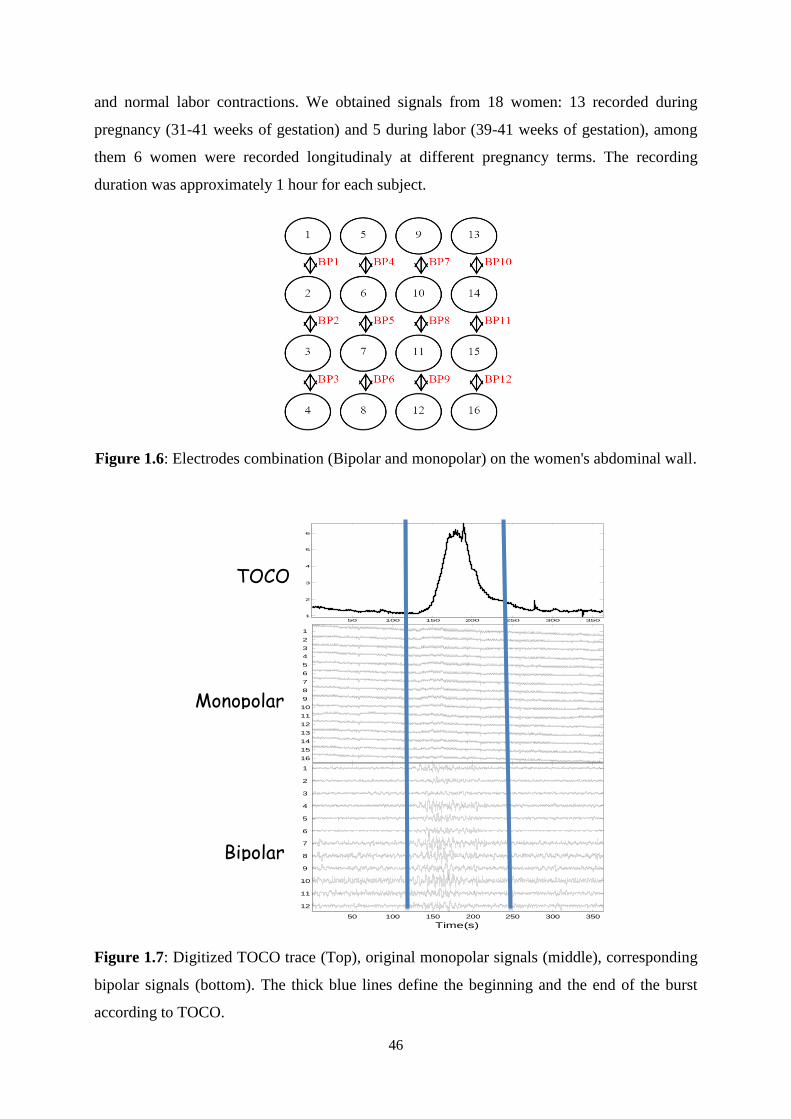
46

and normal labor contractions. We obtained signals from 18 women: 13 recorded during

pregnancy (31-41 weeks of gestation) and 5 during labor (39-41 weeks of gestation), among

them 6 women were recorded longitudinaly at different pregnancy terms. The recording

duration was approximately 1 hour for each subject.

Figure 1.6: Electrodes combination (Bipolar and monopolar) on the women's abdominal wall.

Figure 1.7: Digitized TOCO trace (Top), original monopolar signals (middle), corresponding

bipolar signals (bottom). The thick blue lines define the beginning and the end of the burst

according to TOCO.

50 100 150 200 250 300 350

1

2

3

4

5

6

50 100 150 200 250 300 350

16

15

14

13

12

11

10

9

8

7

6

5

4

3

2

1

50 100 150 200 250 300 350

12

11

10

9

8

7

6

5

4

3

2

1

Time(s)

TOCO trace

Monopolar EHG

Bipolar EHG

47

These raw signals were then segmented, with the help of the scanned and digitized paper

TOCO traces. For verification purpose, we also computed the bipolar signals from monopolar

leads, to check the correctness of the segmentation. Indeed, in the raw monopolar signals the

uterine bursts are corrupted by strong noise and artifacts. We could hardly identify and

segment the uterine bursts by using this signal, even with the help of the TOCO trace. Using

the bipolar signals permitted us to identify and then segment properly the uterine bursts

Figure 1.7.

The monopolar segmented bursts were then filtered by using the CCA-EMD method. At the

end we got 92 pregnancy and 84 labor filtered monopolar bursts related to different

contractions, for each of the 16 monopolar channels.

1.6 Discussion and conclusion

We can conclude from the overview presented above, that the uterus is a complex organ.

Understanding how this organ works might help us to detect the onset of labor as well as to

predict PTL. There are many way of measuring EHG signals, the most used is the abdominal

EHG due to its non-invasiveness. The processing of uterine EMG signals can give us

information about the functioning of the uterus. We expect this information to permit us to

monitor pregnancy and detect labor.

EHG has long been a promising vector of investigation for the detection of preterm labor.

However the classical methods used in the past have not given rise to clinically used

application. Recent efforts using non-linear signal processing and some preliminary work on

uterine activity propagation have given promising results. Thus this thesis focuses on the

analysis of excitability (linear, nonlinear) parameters, propagation (synchronization, direction)

parameters and source(s) localization of the EHG during pregnancy and labor, in order to

move forward to the final aim of this project, deriving objective means for the early detection

of preterm delivery, based on the monitoring of the three physiological phenomenon: cell

excitability, uterine synchronization and source(s) loci.

References




48









[5] J. Terrien, C. Marque, and B. Karlsson, “Spectral characterization of human EHG frequency

components based on the extraction and reconstruction of the ridges in the scalogram,” in 29th

Annual International Conference of the IEEE Engineering in Medicine and Biology

Society(IEEE-EMBC), Lyon, France, Aug. 2007, pp. 1872-1875.




[7] H. Ellis, “Anatomy of the uterus,” Anaesthesia & Intensive Care Medicine, vol. 6, no. 3, pp. 74-

75, Mar. 2005.

[8] Available from: http://www.cancer.gov/cancertopics/pdq/treatment/ovarian-germ-cell/patient.

[9] D. Shier, J. Butler, and R. Lewis, “Hole's Human anatomy and physiology,” New York:

McGraw-Hill, 11th ed., F. Schreiber, Ed., 2001.

[10] A.I. Csapo, “Smooth muscle as a contractile unit,” Phys. Rev. Suppl., vol. 5, pp. 7-33, Jul. 1962.



1993.

[12] R.C. Young, and R.O. Hession, “Three-dimensional structure of smooth muscle in

termpregnant human uterus,” Obstet. Gynecol., vol. 93, no.1, pp. 94-99, Jan. 1999.

[13] K. Chalubinski, J. Deutinger, and G. Bernaschek, “Vaginosonography for recording of

cyclerelated myometrial contractions,” Fertility and sterility, vol. 59, no. 1, pp. 225, Jan. 1993.

[14] R. Merger, J. Levy, and J. Melchior, Précis d'obstétrique, 5th ed., Paris: Masson Ed., 1979.

[15] C. Wood, “Myometrial and tubal physiology,” Blackwell, Ed. Oxford: England, 1972, pp. 324-

375.

[16] F-J. Mercier, H.Bouaziz, D. Benhamou, “«Hypertonie uterine» : conduite a tenir,” in proc.

MAPAR conf, 1997, pp. 99-116.

[17] R. Merger, J. Lévy, and J. Melchior, “Accouchement normal,” in Précis d'Obstétrique, Paris:

Masson Ed., 1985, pp. 115-136.

[18] B. Maria, I. Matheron, and F. Stampf, “Première période du travail,” in Obstétrique, Médecine

Sciences Flammarion, C.D. Papiernik Ed., Pons JC., ed., 1995, pp. 1067-1116.

49

[19] S. Wray, “Uterine contraction and physiological mechanisms of modulation,” American Journal

of Physiology-Cell Physiology, vol. 264, no. 1, pp. C1-C18, Jan. 1993.

[20] R.A. Word, J.T. Stull, M.L. Casey, and K.E. Kamm, “Contractile elements and myosin light

chain phosphorylation in myometrial tissue from nonpregnant and pregnant women,” Journal of

Clinical Investigation, vol. 92, no. 1, pp. 29-37, Jul. 1993.

[21] R. Garfield, and C. Yallampalli, “Structure and function of uterine muscle,” in The uterus,

Cambridge reviews in human reproduction, Cambridge: UK, T. Chard, ed., 1994, pp. 54-93.

[22] R.C. Young, “A computer model of uterine contractions based on action potential propagation

and intercellular calcium waves,” Obstet. Gynecol., vol. 89, no. 4, pp. 604-608, Apr. 1997.

[23] R.C. Young, “Tissue-level signaling and control of uterine contractility: the action potential

calcium wave hypothesis,” J. Soc. Gyneco. Investig., vol. 7, no. 3, pp. 146-52, May-Jun. 2000.

[24] J.M. Marshall, “Regulation of activity in uterine smooth muscle,” Physiol. Rev., vol. 5, pp. 213-

27, Jul. 1962.

[25] R. Caldeyro-barcia, and J.J. Poseiro, “Physiology of the uterine contraction,” Clin. Obstet.

Gynecol., vol. 3, no. 2, pp. 386-408, 1960.

[26] Sims, S., E.E. Daniel, and R. Garfield, Improved electrical coupling in uterine smooth muscle is

associated with increased numbers of gap junctions at parturition. The Journal of general

physiology, 1982. 80(3): p. 353-375.

[27] C. Buhimschi, M.B. Boyle, and R.E. Garfield, “Electrical activity of the human uterus during

pregnancy as recorded from the abdominal surface,” Obstet. Gynecol., vol. 90, no. 1, pp. 102-

11, Jul. 1997.

[28] G.M.J.A. Wolfs, and M.V. Leeuwen, “Electromyographic Observations on the Human Uterus

during Labour,” Acta Obstet. Gynecal. Scand. Suppl., vol. 58, no. 90, pp. 1-62, 1979.

[29] A. Shafik, “Electrohysterogram: study of the electromechanical activity of the uterus in

humans,” Eur. J. Obstet. Gynecol. Reprod. Biol., vol. 73, no. 1, pp. 85-9, May. 1997.

[30] P. Lopes, G. Germain, G. Breart, S. Reitano, R. Le Houezec, and C. Sureau,

“Electromyographical study of uterine activity in the human during labour induced by

prostaglandin F2 alpha,” Gynecol. and obstet. investigation, vol. 17, no. 2, pp. 96-105, 1984.

[31] G. Wolfs, and H. Rottinghuis, “Electrical and mechanical activity of the human uterus during

labour,” Archiv für Gynäkologie, vol. 208, no. 4, pp. 373-385, Jan. 1970.


555, pp. 153-175, Apr-May. 1956.

[33] R. Garfield, M. Blennerhassett, and S. Miller, “Control of myometrial contractility: role and

regulation of gap junctions,” Oxford reviews of reproductive biology, vol. 10, pp. 436-90, 1988.

[34] R.E. Garfield, S. Sims, and E.E. Daniel, “Gap junctions: their presence and necessity in

myometrium during parturition,” Science, vol. 198, no. 4320, pp. 958-60, Dec. 1977.

50

[35] H. Eswaran, H. Preissl, P. Murphy, J.D. Wilson, and C.L. Lowery, “Spatial-temporal analysis of

uterine smooth muscle activity recorded during pregnancy,” in 27th Annual International

Conference of the IEEE Engineering in Medicine and Biology Society (IEE-EMBC), Shanghai,

China, Jan. 2006, pp. 6665-6667.


[37] M. Baggish, R. Valle, and H. Guedj, “Hysteroscopy: Visual Perspectives of Uterine Anatomy,

Physiology & Pathology,” 3rd Ed., Lippincott Williams & Wilkins, Philadelphia: USA, 2007.



[39] G. Bréart, B. Blondel, P. Tuppin, H. Grandjean, and M. Kaminski, “Did preterm deliveries

continue to decrease in France in the 1980s?,” Pediatric and Perinatal Epidemiology, vol. 9, no.

3, pp. 296-306, Jul. 1995.

[40] P. Olsén, E. Läärä, P. Rantakallio, M.-R. Järvelin, A. Sarpola, and A.-L. Hartikainen,

“Epidemiology of preterm delivery in two birth cohorts with an interval of 20 years,” American

Journal of Epidemiology, vol. 142, no. 11, pp. 1184-1193, Aug. 1995.

[41] B. Blondel, G. Bréart, Ch. du Mazaubrun, and G. Badeyan, “Santé publique la situation

périnatale en France,” J. Gynecol. Obstet. Biol. Reprod., vol. 26, no. 8, pp. 770-780, Dec. 1997.

[42] B. Blondel, N. Lelong, M. Kermarrec, and F. Goffinet, “La santé périnatale en France

métropolitaine de 1995 à 2010. Résultats des enquêtes nationales périnatales,” La Revue Sage

Femme, vol. 11, no. 3, pp. 128-143, Jun. 2012.

[43] M.I. Heaman, A.E. Sprague, and P.J. Stewart, “Reducing the preterm birth rate: A population

health strategy,” J. of Obstet., Gynecol., & Neonat. Nursing, vol. 30, no. 1, pp. 20-29, Jan. 2001.

[44] J.C. Morrison, J.R. Allbert, B.N. McLaughlin, N.S. Whitworth, W.E. Roberts, and R.W. Martin,

“Oncofetal fibronectin in patients with false labor as a predictor of preterm delivery,” American

journal of obstetrics and gynecology,” vol. 168, no. 2, pp. 538-542, Feb. 1993.

[45] M.A. Williams, D.E. Hickok, R.W. Zingheim, R. Mittendorf, J. Kimelman, and B.S. Mahony,

“Low birth weight and preterm delivery in relation to early-gestation vaginal bleeding and

elevated maternal serum alpha-fetoprotein,” Obstetrics & Gynecology, vol. 80, no. 5, pp. 745-

749, Nov. 1992.

[46] M. McLean, A. Bisits, J. Davies, R. Woods, P. Lowry, and R. Smith, “A placental clock

controlling the length of human pregnancy,” Nature medicine, vol. 1, no. 5, pp. 460-463, May.

1995.

[47] J.D. Iams, “Prediction and early detection of preterm labor,” Obstet. Gynecol., vol. 101, no. 2,

pp. 402-12, Feb. 2003.

[48] R.K. Creasy, “Preterm birth prevention: where are we?,” American journal of obstetrics and

gynecology, vol. 168, no. 4, pp. 1223-1230, Apr. 1993.

51

[49] D.C. Dyson, K.H. Danbe, J.A. Bamber, Y.M. Crites, D.R. Field, J.A. Maier, L.A. Newman,

D.A. Ray, D.L. Walton, and M.A. Armstrong, “Monitoring women at risk for preterm labor,”

New England J. Med., vol. 338, no. 1, pp. 15-9, Jan. 1998.

[50] D. Schlembach, W.L. Maner, R.E. Garfield, and H. Maul, “Monitoring the progress of

pregnancy and labor using electromyography,” Eur. J. Obstet. Gynecol. Reprod. Biol., vol. 144,

no. 1, pp. S33-9, May. 2009.

[51] R. Romero, R. Gomez, and W. Sepulveda, “The uterine cervix, ultrasound and prematurity,”

Ultrasound. Obstet. Gynecol., vol. 2, no. 6, pp. 385-8, Nov. 1992.

[52] A.M. Germain, G.J. Valenzuela, M. Ivankovic, C.A. Ducsay, C. Gabella, and M. Serón-Ferré,

“Relationship of circadian rhythms of uterine activity with term and preterm delivery,” Am. J.

Obstet. Gynecol., vol. 168, no. 4, pp. 1271-7, Apr. 1993.

[53] H. Eswaran, H. Preissl, J.D. Wilson, P. Murphy, S.E. Robinson, and C.L. Lowery, “First

magnetomyographic recordings of uterine activity with spatial-temporal information with a 151-

channel sensor array,” Am. J. Obstet. Gynecol., vol. 187, no. 1, pp. 145-51, Jul. 2002.

[54] O. Bode, “Das elektrohysterogramm,” Arch. Gyndk, vol. 28, no. 1, pp. 123-128, 1931.

[55] A. Verhoeff, “Myometrial Contractility and Gap Junctions: An Experimental Study in

Chronically Instrumented Ewes,” Erasmus University Rotterdam, pp. 1-87, Nov. 1985.

[56] H. Maul, W.L. Maner, G.R. Saade, and R.E. Garfield, “The physiology of uterine contractions,”

Clinics in perinatology, vol. 30, no. 4, pp. 665-676, Dec. 2003.

[57] L. Dill, and R. Maiden, “The electrical potentials of the human uterus in labor,” American

journal of obstetrics and gynecology, vol. 52, no. 5, pp. 735-745, Nov. 1946.

[58] C.M. Steer, and G. Hertsch, “Electrical activity of the human uterus in labor; the

electrohysterograph,” American journal of obstetrics and gynecology, vol. 59, no.1, pp. 25-40,

Jan. 1950.

[59] E.H. HON, and C.D. DAVIS, “Cutaneous and uterine electrical potentials in labor-an

experiment,” Obstetrics & Gynecology, vol. 12, no. 1, pp. 47-53, Jul. 1958.

[60] C. Sureau, J. Chavinié, and M. Cannon, “L‟electrophysiologie uterine,” Bull Fed Soc Gynecol

Obstet, vol. 17, pp. 79-140, 1965.





2, pp. 149-53, Apr. 2001.

[63] S. Larks, N. Assali, D. Morton, and W. Selle, “Electrical activity of the human uterus in labor,”

Journal of Applied Physiology, vol. 10, no. 3, pp. 479-483, May. 1957.

52

[64] H.W. Hsu, J.P. Figueroa, M.B. Honnebier, R. Wentworth, P.W. Nathanielsz, “Power spectrum

analysis of myometrial electromyogram and intrauterine pressure changes in the pregnant rhesus

monkey in late gestation,” Am. J. Obstet. Gynecol., vol. 161, no. 2, pp. 467-73, Aug. 1989.

[65] N. Val, B. Dubuisson, and F. Goubel, “Aide au diagnostic de l‟accouchement par

l‟électromyogramme abdominal: sélection de caractères,” in Reconnaissance de formes,

intelligence artificielle, vol. 3, pp. 42-50, 1979.







[68] M. Diab, C. Marque, and M. Khalil, “An unsupervised classification method of uterine

electromyography signals: classification for detection of preterm deliveries,” Journal of

Obstetrics and Gynaecology Research, vol. 35, no. 1, pp. 9-19, Feb. 2009.



[70] P. Carre, H. Leman, C. Fernandez, and C. Marque, “Denoising of the uterine EHG by an

undecimated wavelet transform,” IEEE Trans. Biomed. Eng., vol. 45, no. 9, pp. 1104-13, Sep.

1998.







[73] M. Khalil, and J. Duchêne, “Uterine EMG analysis: a dynamic approach for change detection

and classification,” IEEE Trans. Biomed. Eng., vol. 47, no. 6, pp. 748-56, Jun. 2000.

[74] C. Marque, H. Leman, M.L. Voisine, J. Gondry, and P. Naepels, “Processing of uterine

electromyogram for contraction characterization during pregnancy: Traitement de

l'electromyogramme uterin pour la caracterisation des contractions pendant la grossesse,” RBM-

News, vol. 21, no. 9, pp. 200-211, Dec. 1999.

[75] J. Duchêne, D. Devedeux, S. Mansour, and C. Marque, “Analyzing Uterine EMG: Tracking

Instantaneous Burst Frequency,” IEEE Eng. Med. Biol. Mag., vol. 14, no. 2, pp. 125-131, Mar-

Apr. 1995.

53

[76] E. Oczeretko, A. Kitlas, J. Swiatecka, M. Borowska, and T. Laudanski, “Nonlinear dynamics in

uterine contractions analysis,” in Fractals in Biology and Medicine, Birkhäuser Basel, Springer,

2005, pp. 215-222.

[77] I.A. Rezek, and S.J. Roberts, “Stochastic complexity measures for physiological signal

analysis,” IEEE Trans. on Biomed. Eng., vol. 45, no. 9, pp. 1186-1191, Sep. 1998.

[78] J. Vrhovec, “Evaluating the progress of the labour with sample entropy calculated from the

uterine EMG activity,” Elektrotehniski vestnik-Electrotechnical Review, vol. 76, no. 4, pp. 165-

170, Jan. 2009.

[79] W.L. Maner, L.B. MacKay, G.R. Saade, and R.E. Garfield, “Characterization of abdominally

acquired uterine electrical signals in humans, using a non-linear analytic method,” Med. Biol.

Eng. Comput., vol. 44, no. 1-2, pp. 117-23, Mar. 2006.

[80] M. Sabry-Rizk, W. Zgallai, E.R. Carson, P. Hardiman, A. MacLean, and K.T.V. Grattan,

“Nonlinear dynamic tools for characterizing abdominal electromyographic signals before and

during labour,” Trans. of the instit. of Measu. and Cont., vol. 22, no. 3, pp. 243-270, Aug. 2000.

[81] C. Marque, “Analyse de la dynamique des contractions uterines par électromyographie

abdominale,” Ph.D. dissertation, Dept. Génie biomédical, Université de Technologie de

Compiègne, Compiègne, France, 1987.




[83] B. Karlsson, J. Terrien, V. Gudmundsson, T. Steingrimsdottir, and C. Marque, “Abdominal

EHG on a 4 by 4 grid: mapping and presenting the propagation of uterine contractions,” in Proc.

11th Mediterranean Conference on Medical and Biological Engineering and Computing

(MEDICON), Ljubljana, Slovenia, 2007, pp. 139-143.

[84] W. Jiang, G. Li, and L. Lin, “Uterine electromyogram topography to represent synchronization

of uterine contractions,” International Journal of Gynecology & Obstetrics, vol. 97, no. 2, pp.

120-124, May. 2007.

[85] J. Terrien, C. Marque, J. Gondry, T. Steingrimsdottir, and B. Karlsson, “Uterine

electromyogram database and processing function interface: An open standard analysis platform

for electrohysterogram signals,” Comput. in bio. & med., vol. 40, no. 2, pp. 223-230, Feb. 2010.




[87] J. Terrien, M. Hassan, C. Marque, and B. Karlsson, “Use of piecewise stationary segmentation

as a pre-treatment for synchronization measures,” in Proc. IEEE Eng. Med. Biol. Soc. Conf.

2008, Vancouver, BC, Aug. 2008, pp. 2661-2664.

54

[88] J. Terrien, G. Germain, C. Marque, and B. Karlsson, “Bivariate piecewise stationary

segmentation; improved pre-treatment for synchronization measures used on non-stationary

biological signals,” Medical engineering & physics, vol. 35, no. 8, pp. 1188-96, Aug. 2013.

[89] J. Terrien, T. Steingrimsdottir, C. Marque, and B. Karlsson “Synchronization between EMG at

Different Uterine Locations Investigated Using Time-Frequency Ridge Reconstruction:

Comparison of Pregnancy and Labor Contractions,” EURASIP J. Adv. Signal Process., vol.

2010, pp. 1-10, Jun. 2010.

[90] J. G. Planes, J. P. Morucci, H. Grandjean, and R. Favretto, “External recording and processing

of fast electrical activity of the uterus in human parturition,” Med Biol Eng Comput, vol. 22, pp.

585-91, Nov 1984.

[91] W.J. Lammers, H. Mirghani, B. Stephen, S. Dhanasekaran, A. Wahab, M.A.H. Al Sultan, and F.

Abazer, “Patterns of electrical propagation in the intact pregnant guinea pig uterus,” Am. J.

Physiol. Regul. Integr. Comp. Physiol., vol. 294, no. 3, pp. R919-28, Mar. 2008.



Gynecol., vol. 200, no. 1, pp. 54.e1–54.e7, Jan. 2009.

[93] C. Alvarez, and S. Reynolds, “A better understanding of uterine contractility through

simultaneous recording with an internal and a seven channel external method,” Surgery,

gynecology & obstetrics, vol. 91, no. 6, pp. 641-650, Dec. 1950.



745-61, Jun. 2009.

[95] E. Mikkelsen, P. Johansen, A. Fuglsang‐Frederiksen, and N. Uldbjerg, “Electrohysterography of


Scandinavica, vol. 92, no. 9, pp. 1070-1078, Sept. 2013.

[96] A. Diab, M. Hassan, S. Boudaoud, C. Marque, and B. Karlsson, “Nonlinear estimation of

coupling and directionality between signals: Application to uterine EMG propagation,” in Proc.

IEEE Eng. Med. Biol. Soc. Conf. 2013, Osaka, Japan, Jul. 2013, pp. 4366-4369.

[97] J.D. López, V. Litvak, J.J. Espinosa, K. Friston, and G.R. Barnes, “Algorithmic procedures for

Bayesian MEG/EEG source reconstruction in SPM,” NeuroImage, vol. 48, pp. 476-487, Jan.

2014.

[98] J. Mattout, C. Phillips, W.D. Penny, M.D. Rugg, and K.J. Friston, “MEG source localization

under multiple constraints: An extended Bayesian framework,” NeuroImage, vol. 30, no. 3, pp.

753-767, Apr. 2006.

[99] J. Alberola-Rubio, G. Prats-Boluda, Y. Ye-Lina, J. Valerob, A. Peralesb, and J. Garcia-Casado,

“Comparison of non-invasive electrohysterographic recording techniques for monitoring uterine

dynamics,” Medical engineering & physics, vol. 35, no. 12, pp. 1736-1743, Dec. 2013.

55

[100] J. Terrien, C. Marque, G. Germain, and B. Karlsson, “Sources of bias in synchronization

measures and how to minimize their effects on the estimation of synchronicity: application to

the uterine electromyogram,” in Rec. Adv. in Biom. Eng., Ganesh R Naik Ed., 2009, pp. 73-100.

[101] J.-N. Helal, and P. Bouissou, “The spatial integration effect of surface electrode detecting

myoelectric signal,” IEEE Trans. on Biomed. Eng., vol. 39, no. 11, pp. 1161-1167, Nov. 1992.

[102] S. Mansour, J. Duchêne, G. Germain, and C. Marque, “Uterine EMG: Experimental and

mathematical determination of the relationship between internal and external recordings,” in

13th Annual International Conference of the IEEE Engineering in Medicine and Biology Society

(IEEE-EMBC), Orlando, FL, USA, Oct/Nov. 1991, pp. 485-486.

[103] L. Lindström, and I. Petersen, “Power spectrum analysis of EMG signals and its applications,”

Prog. Clin. Neurophysiol., vol. 10, pp. 1-51, 1983.

[104] M. Hassan, S. Boudaoud, J. Terrien, B. Karlsson, and C. Marque, “Combination of Canonical

Correlation Analysis and Empirical Mode Decomposition applied to denoise the labor

electrohysterogram,” IEEE Trans. Biomed. Eng., vol. 85, no. 9, pp. 2441-2447, Sep. 2011.

56

Chapter 2: Excitability analysis using nonlinear methods

2.1 Introduction

One of the most common ways to obtain information on neurophysiologic systems is to study

the features of the signal(s) using time series analysis techniques. They traditionally rely on

linear methods in both time and frequency domains [1], such as peak frequency of signals

PSD [2], and burst energy [3]. Unfortunately, these methods cannot give information about

purely nonlinear features of the signal.

Due to the intrinsic nonlinearity of most biological systems, these nonlinear features may be

present in physiological data and even be a characteristic of major interest. Indeed, the

nonlinear analysis may give information about the underlying physiological processes, many

of which have complex behavior. Monovariate nonlinear time series analysis methods were

first applied to neurophysiological data about two decades ago [4]. Recently, much attention

has been paid to the use of nonlinear analysis techniques for the characterization of biological

signals [5]. They have been widely applied to EEG signals since these signals are highly

nonlinear and nonstationary. Among those applications we can cite: study of the anesthetic

drug effect during anesthesia by using Approximate entropy [6], measure of the depth of

anesthesia using Detrended fluctuation analysis [7], and sleep stages study [8], study of the

effect of antipsychotics on EEG complexity in drug-naive schizophrenia using multiscale

entropy [9]. Nonlinear analysis were also used in cardiovascular dynamic analysis [10], study

of cardiovascular ageing [11], prediction of paroxysmal atrial fibrillation [12], and fetal

heart rate analysis [13]. MEG was also a field for nonlinear analysis application such as for

the analysis of Alzheimer disease [14]. Complexity of striated muscle EMG signals was also

measured by using entropy based methods (Fuzzy Entropy, Approximate Entropy, Sample

entropy) [15]. Several measures have thus been proposed to detect nonlinear characteristics in

time series. The performances of these methods are often compared with their results on

surrogate data, which provides a rigorous framework for detecting nonlinearity. Multiple

surrogates and their z-score are used to statistically test the presence or absence of non-

linearity in time series. The z-score itself has sometimes been used as a measure of

nonlinearity [5, 16].

57

The uterus is a not well-understood organ. It is deceptively simple in structure but its

behavior, as observed by electromyography (electrohysterogram, EHG), when it moves from

pregnancy towards labor, indicates that there are numbers of interconnected control systems

involved in its functioning (electric, hormonal, mechanical). Nonlinear characteristics have

been observed in the EHG and some success has been achieved by using these characteristics

to obtain information that is potentially clinically useful [5, 16-17]. Recently, several

applications of nonlinear analysis methods have been done on EHG signals. We can cite here

the use of Sample Entropy [18], Lempel-Ziv complexity [19] and Approximate entropy [20].

In most of these studies the authors have reported some practical disadvantages of the

methods, like the huge calculation time due to using surrogates analysis, or promising but

inconclusive results due to the small databases available.

However, whatever the studied signal, the sensitivity of nonlinear methods to the actual

nonlinearity level, and to some usual preprocessing steps (decimation, filtering), as well as

their robustness to noise has rarely been evaluated in the past. While surrogates are important

tools to rigorously detect nonlinearity, their usefulness for evaluating the level of existing

nonlinearity is not clear, and their usefulness is limited by their complexity and highly time

consuming computation.

This chapter presents a work that extends previous work done in our team, which deals with

the comparison between Approximate Entropy, Correntropy and Time reversibility [16]. In

the present work, we compare new methods and also use a much larger database of real

signals than during the previous work. In addition, we propose in this work to complete this

comparison by the investigation of the method‟s sensitivity to the varying complexity of

signals and then to their SNR. We also studied the effect of two usual preprocessing steps,

decimation (or down sampling) and filtering, on the performances of the methods. Papers that

investigate the effect of preprocessing are rare in the EHG literature. We found one example

of this systematic analysis for Sample entropy [21] only. None of these topics has previously

been considered in our team.

Four nonlinear methods from three nonlinear families: Statistic family (Time reversibility

[22]), Predictability family (Sample Entropy [23], Delay Vector Variance [24]) and Chaos

theory family (Lyapunov Exponents [25]) were tested in this work. Sensitivity of these

methods to the complexity degree (CD) of signal as well as robustness analysis were made on

a Henon model synthetic signals where CD can be controlled. The sensitivity to CD was first

58

studied by using the direct value provided by the method. It was then studied by using

surrogates and z-score, as this measure permits to evaluate the nonlinearity. We try in this

study to evidence which methods are the most sensitive to the change of signal complexity. A

second objective was to determine whether the use of surrogates give better overall results

than the direct application of the methods. This is also of major practical importance for

clinical application, as the generation of surrogates is computationally very time consuming.

The methods were compared using the MSE (Mean Square Error) of the Monte Carlo

instances of the signal. Finally, these non-linear methods are applied to real EHG signals, and

used to discriminate pregnancy and labor contractions. The methods‟ discriminating power is

compared to that of three well known linear characteristics based on the frequency content of

the signal: Mean Power Frequency (MPF), Peak Frequency (PF) and Median Frequency

(MF). We also tested, on real EHG signals, the sensitivity of these methods to decimation and

filtering, by comparing the effect of these two preprocessing techniques (with and without

down sampling and filtering) on method performances, for the discrimination between

pregnancy and labor contractions.

2.2 Materials and methods

2.2.1 Data

2.2.1.1 Synthetic signals

In this work, we used the Henon nonlinear dynamic model because the complexity degree of

this model can be easily controlled. The Henon map is a well-known two-dimensional

discrete-time system given by

𝑌𝑡+1 = 𝑐 − 𝑌𝑡2 + 𝐶𝐷 ∗ 𝑋𝑡 ,

𝑋𝑡+1 = 𝑌𝑡 ,

where Yt and Xt represent dynamical variables, CD is the complexity degree and c is the

dissipation parameter. In this work, we use c = 1 as in [26] and CD ϵ [0, 1] to change the

model complexity [27] (Figure 2.1). The number of generated points is fixed to 1000.

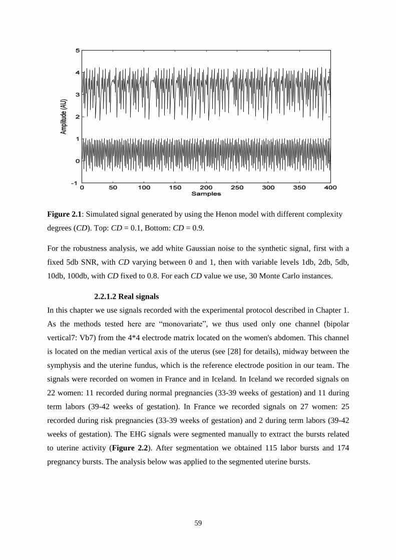
59

Figure 2.1: Simulated signal generated by using the Henon model with different complexity

degrees (CD). Top: CD = 0.1, Bottom: CD = 0.9.

For the robustness analysis, we add white Gaussian noise to the synthetic signal, first with a

fixed 5db SNR, with CD varying between 0 and 1, then with variable levels 1db, 2db, 5db,

10db, 100db, with CD fixed to 0.8. For each CD value we use, 30 Monte Carlo instances.

2.2.1.2 Real signals

In this chapter we use signals recorded with the experimental protocol described in Chapter 1.

As the methods tested here are “monovariate”, we thus used only one channel (bipolar

vertical7: Vb7) from the 4*4 electrode matrix located on the women's abdomen. This channel

is located on the median vertical axis of the uterus (see [28] for details), midway between the

symphysis and the uterine fundus, which is the reference electrode position in our team. The

signals were recorded on women in France and in Iceland. In Iceland we recorded signals on

22 women: 11 recorded during normal pregnancies (33-39 weeks of gestation) and 11 during

term labors (39-42 weeks of gestation). In France we recorded signals on 27 women: 25

recorded during risk pregnancies (33-39 weeks of gestation) and 2 during term labors (39-42

weeks of gestation). The EHG signals were segmented manually to extract the bursts related

to uterine activity (Figure 2.2). After segmentation we obtained 115 labor bursts and 174

pregnancy bursts. The analysis below was applied to the segmented uterine bursts.

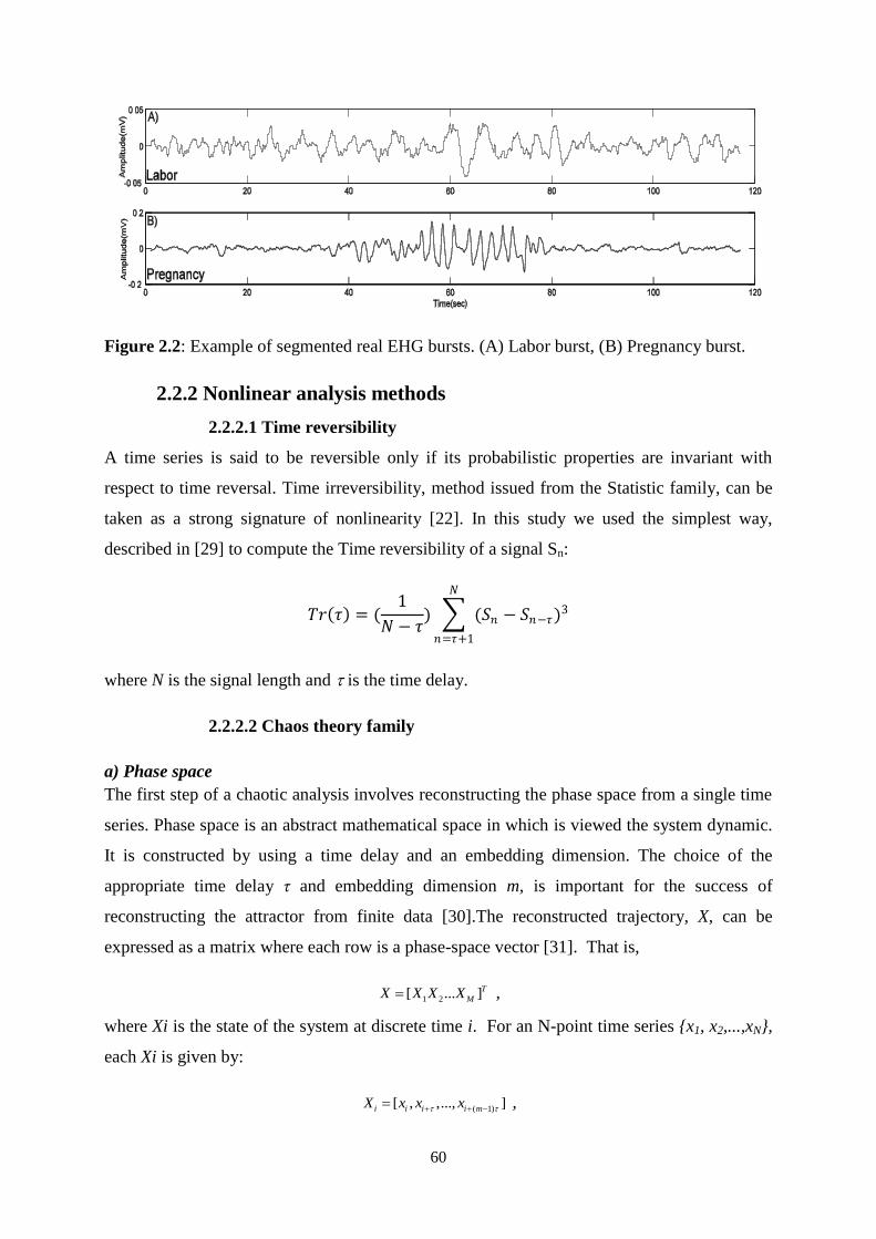
60

Figure 2.2: Example of segmented real EHG bursts. (A) Labor burst, (B) Pregnancy burst.

2.2.2 Nonlinear analysis methods

2.2.2.1 Time reversibility

A time series is said to be reversible only if its probabilistic properties are invariant with

respect to time reversal. Time irreversibility, method issued from the Statistic family, can be

taken as a strong signature of nonlinearity [22]. In this study we used the simplest way,

described in [29] to compute the Time reversibility of a signal Sn:

𝑇𝑟 𝜏 = (1

𝑁 − 𝜏) (𝑆𝑛 − 𝑆𝑛−𝜏)3

𝑁

𝑛=𝜏+1

where N is the signal length and is the time delay.

2.2.2.2 Chaos theory family

a) Phase space

The first step of a chaotic analysis involves reconstructing the phase space from a single time

series. Phase space is an abstract mathematical space in which is viewed the system dynamic.

It is constructed by using a time delay and an embedding dimension. The choice of the

appropriate time delay τ and embedding dimension m, is important for the success of

reconstructing the attractor from finite data [30].The reconstructed trajectory, X, can be

expressed as a matrix where each row is a phase-space vector [31]. That is,

,

where Xi is the state of the system at discrete time i. For an N-point time series {x1, x2,...,xN},

each Xi is given by:

,

1 2[ ... ]T

MX X X X

( 1)[ , ,..., ]i i i i mX x x x

61

where τ is the time lag or reconstruction delay, and m is the embedding dimension. Thus, X is

an M×m matrix, and the constants m, M, τ, and N are related by:

M = N - (m - 1)τ

As previously stated, the good reconstruction of the phase space depends on the two

parameters, τ and m. We thus chose an optimal value for each one of these parameters. For the

time delay, τ, we use the first local minimum of the average mutual information between the

set of measurements X(i) and X(i + τ). Mutual information measures the general dependence

of two variables [32].

We estimated the minimum embedding dimension, m, by using an algorithm proposed by

Kennel et al. [33]. The algorithm is based on the idea that, when passing from dimension m to

dimension m+1, one can differentiates points on the orbit that are true neighbors from those

that are false ones. A false neighbor is a point in the data set that is identified as a neighbor

solely because the attractor is viewed in a too small embedding space. When the embedding

dimension is large enough, all neighbors of every attractor point in the multivariate phase

space will be true neighbors [30].

b) Lyapunov exponents

Lyapunov exponent (LE) is inspired from the Chaos theory. It is a quantitative indicator of

system dynamics, which characterizes the average convergence or divergence rate between

adjacent tracks in phase space [25]. We used the way described in [34] to compute LE:

Where ∥ 𝛥𝑦0∥ and ∥ 𝛥𝑦𝑡 ∥ represent the Euclidean distances between two states of the

system, respectively to an arbitrary time t0 and a later time t.

2.2.2.3 Predictability family

a) Sample entropy

Sample Entropy (SampEn) is chosen from the Predictability family. It is the negative natural

logarithm of the conditional probability that a dataset of length N, having repeated itself for m

samples within a tolerance r, will also repeat itself for m+1 samples. Thus, a lower value of

SampEn indicates more regularity in the time series [23]. We used the way described in [18]

to compute SampEn :

0

00

1lim lim log ,

ty

y yt t

62

For a time series of N points, x1, x2, . . . ,xN, we define subsequences, also called template

vectors, of length m, given by: yi(m) = (xi, xi+1,..., xi+m−1) where i = 1, 2,...,N-m+1.

Then the following quantity is defined: 𝐵𝑖𝑚(𝑟) as (N-m-1)

−1 times the number of vectors 𝑋𝑗

𝑚

within r of 𝑋𝑖𝑚 , where j ranges from 1 to N-m, and j≠i, to exclude self-matches, and then

define:

𝐵𝑚 𝑟 =1

𝑁 −𝑚 𝐵𝑖

𝑚(𝑟)

𝑁−𝑚

𝑖=1

Similarly, we define 𝐴𝑖𝑚 (𝑟) as (N-m-1)

-1 times the number of vectors 𝑋𝑗

𝑚+1 within r of 𝑋𝑖𝑚+1,

where j ranges from 1 to N-m, where j≠i, and set

𝐴𝑚 𝑟 =1

𝑁 −𝑚 𝐴𝑖

𝑚 (𝑟)

𝑁−𝑚

𝑖=1

The parameter SampEn(m,r) is then defined as 𝑙𝑖𝑚𝑁→∞ − 𝑙𝑛 𝐴𝑚 𝑟 𝐵𝑚 𝑟 , which can be

estimated by the statistic:

𝑆𝑎𝑚𝑝𝐸𝑛 𝑚, 𝑟,𝑁 = − ln 𝐴𝑚 𝑟 𝐵𝑚 𝑟

where N is the length of the time series, m is the length of sequences to be compared, and r is

the tolerance for accepting matches.

b) Delay vector variance

The delay vector variance (DVV) method belongs to the Predictability method family. It is

used for detecting the presence of determinism and nonlinearity in a time series and is based

upon the examination of local predictability of a signal [24]. We use the measure of

unpredictability 𝜎∗2 described in [35]:

Time series can be represented conveniently in the phase space by using time delay

embedding. When time delay is embedded into a time series, it can be represented by a set of

delay vectors (DVs) of a given dimension. If m is the dimension of the delay vectors then it

can be expressed as X (k) =[x (k-mτ) …x (k-τ)], where τ is the time lag. For every DV X (k), there

is a corresponding target, namely the next sample xk. A set βk (m, d) is generated by grouping

those DVs that are within a certain Euclidean distance d to DV X(k). This Euclidean distance

will be varied in a standardized manner with respect to the distribution of pair-wise distances

63

between DVs. For a given embedding dimension m, a measure of unpredictability σ*2

(target

variance) is computed over all sets of βk.

The mean μd and the standard deviation σd are computed over all pair-wise Euclidean

distances between DVs given by 𝑥 𝑖 − 𝑥 𝑗 (𝑖 ≠ 𝑗). The sets βk (m, d) are generated such

that 𝛽𝑘 = 𝑥(𝑖)\ 𝑥 𝑘 − 𝑥 𝑗 ≤ 𝑑 i.e., sets which consist of all DVs that lie closer to X(k)

than a certain distance d, taken from the interval [μd-nd*σd; μd+nd*σd] where nd is a parameter

controlling the span over which to perform DVV analysis.

For every set βk(m, d) the variance of the corresponding targets σk2(m, d) is computed. The

average over the N sets βk(m, d) is divided by the variance of the time series signal 𝜎𝑥2 , giving

thus the inverse measure of predictability, namely target variance σ*2.

𝜎∗2 = 1 𝑁 𝜎𝑘

2𝑁𝑘=1

𝜎𝑥2

2.2.3 Surrogates

To compare method ability to detect non-linearity in a signal, their results are often compared

with the ones obtained on surrogate data. To obtain the surrogate data one has to shuffle the

original signal so that the surrogate presents linear properties but keeps the other

characteristics of the signal. This provides a rigorous framework for detecting nonlinearity, by

using a statistical test to compare the results obtained from the original signals and from the

surrogates. The application of a method on multiple surrogates, coupled with a statistical test

on their z-score, permits to test the presence or absence of non-linearity in a time series. As

the z-score itself is normalized with respect to the standard deviation of the results on the

surrogates, it has sometimes been used as a measure of nonlinearity in its own right. In this

work we use both the direct result of the analyzed methods and the ones obtained when

coupled with the z-score, in order to compare which one is the best for our purposes. We

present below the details of the surrogates and z-score computation used in this work.

2.2.3.1 Surrogates

Three main algorithms exist for generating surrogate data: Fourier Transformed (FT), Fourier

Shuffled (FS) and Iterative Amplitude Adjusted Fourier Transformed (IAAFT). We introduce

below the IAAFT algorithm as it preserves more accurately the power spectrum than the FS

surrogate. Furthermore, the IAAFT algorithm (Figure 2.3) completely preserves the

histogram of the original time series [36].

64

Figure 2.3: The IAAFT algorithm. Left: block diagram of the algorithm; middle: original

(upper), intermediate and surrogate (lower) time series; right: time series histograms [37].

The IAAFT algorithm consist of the following steps:

1. Estimate the power spectrum of the original time series by the Fourier Transform.

2. Make a FS surrogate data of the original time series by shuffling the original data and

keeping the same rank order as the FT surrogate data (inverse Fourier Transform of the

spectrum estimated in the previous step) after a phase randomization. Although the FS

surrogate completely preserves the empirical histogram, it cannot completely preserve

the power spectrum as the FT surrogate.

3. Apply Fourier Transform to the FS surrogate. Here, the power spectrum is replaced by

the one of the original time series, estimated at the first step, but the phase of the FS

surrogate spectrum is preserved.

65

4. Apply inverse Fourier Transform to the data obtained at the third step. Although the

generated time series has the same power spectrum as the original time series, its

empirical histogram is different from the original one.

5. In order to preserve the histogram of the original data, the original time series is re-

ordered to have the same rank order than the generated time series obtained at the fourth

step. The re-ordered original time series is an IAAFT surrogate.

6. If the discrepancy of the power spectrum between the original and the IAAFT surrogate

obtained in the previous step is not small enough, repeat the above steps by replacing

the FS surrogate by the IAAFT surrogate in the third step. Large numbers of repetitions

of these steps preserve more accurately the power spectrum of the original data than the

only FS surrogate does [36].

2.2.3.2 Null hypothesis

The most commonly used null hypothesis considers that a given time series is generated by a

Gaussian linear stochastic process and collected through a nonlinear measurement static

function. Thus, well-designed surrogates must have the same linear properties as the original

signal (frequency content, autocorrelation and amplitude distribution…). However, any

underlying nonlinear dynamic structure within the original data is altered in the surrogates by

phase randomization [16]. The surrogate-generated data are compared to the original data by a

discriminant nonlinear measure. If the value of the measure for the original time series lies

within the distribution of surrogate values, with a level of confidence, the null hypothesis is

accepted and the original series is considered as linear. If the measurement gives quite

different values for the original series and the surrogates, the null hypothesis is rejected and

the original series is considered as non-linear.

2.2.3.3 Statistical test for nonlinearity (z-score)

If we want the power of the statistical test to be α, we have to design at least a number of

(1/α-1) sets of surrogate data. We have to generate a set of M surrogate data for every

synthetic or real EHG signal, in order to test the null hypothesis. The null hypothesis is

rejected at the 0.05 significance level, if the discriminating statistic (value of method) q0, from

an applied nonlinear method on the original data set, is statistically different from statistics

q1,…,qM of the M surrogates [38].

To compare the original and surrogate series, discriminative statistics are calculated for both

series. The statistics of significance z-score is

66

𝑍𝑠𝑐𝑜𝑟𝑒 = 𝑞0 − 𝑞𝑠 𝑖

𝜎𝑞 𝑖

where q0 stands for the statistic on the original time series, 𝑞𝑠 𝑖 stands for the mean and

σq(i) for the standard deviation of the statistic on the surrogate time series, for i=1,2,…,M. For

α=0.05, the critical value of z-score is 1.96. Therefore, the null hypothesis is rejected when z-

score >1.96, with a 0.05 significance level and the original signal is thus considered as

nonlinear [38].

2.2.4 Mean square error

Methods are compared by using the Mean Square Error (MSE), which is the estimate of the

square of the standard deviation (σ2) calculated, for the example of Time reversibility, in the

following way:

𝑀𝑆𝐸(𝐶𝐷) =1

𝑛 𝑇𝑟 𝐶𝐷 − 𝑇𝑟𝑖

𝐶𝐷 2

𝑛

𝑖=1

where n is the number of Monte Carlo instances of signal generated by the model, Tr(CD)

is the

mean of Time reversibility over the n Monte Carlo trials on a complexity degree CD. We

compute the MSE for each value of complexity degree CD.

2.3 Results

2.3.1 Results for synthetic signals

2.3.1.1 Evolution with CD

In this section we study the evolution of the values generated by the four methods (Time

reversibility -TR-, Lyapunov exponent -LE-, Sample Entropy –SampEn-, delay vector

variance -DVV) while varying the complexity degree (CD) of the Henon synthetic model, in

four cases: 1) direct application of the method with no added noise, 2) direct application of the

method with added noise, 3) using surrogates with no added noise and 4) using surrogates

with added noise. The added noise is a white Gaussian noise with a fixed SNR of 5 db (SNR

close to the SNR of real signals) and due to the limitation of EHG bandwidth, while the CD of

the Henon model varies between 0 and 1. Our first objective is to test the sensitivity of

methods to varying CD of the signal, with and without noise. Our second objective is to test if

the use of surrogates improves the method sensitivity to complexity or not. Thus if we can

find a method that yields good sensitivity without using surrogates, then we can reduce the

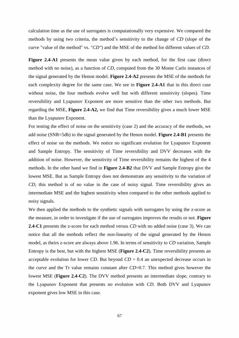
67

calculation time as the use of surrogates is computationally very expensive. We compared the

methods by using two criteria, the method‟s sensitivity to the change of CD (slope of the

curve "value of the method" vs. "CD") and the MSE of the method for different values of CD.

Figure 2.4-A1 presents the mean value given by each method, for the first case (direct

method with no noise), as a function of CD, computed from the 30 Monte Carlo instances of

the signal generated by the Henon model. Figure 2.4-A2 presents the MSE of the methods for

each complexity degree for the same case. We see in Figure 2.4-A1 that in this direct case

without noise, the four methods evolve well but with different sensitivity (slopes). Time

reversibility and Lyapunov Exponent are more sensitive than the other two methods. But

regarding the MSE, Figure 2.4-A2, we find that Time reversibility gives a much lower MSE

than the Lyapunov Exponent.

For testing the effect of noise on the sensitivity (case 2) and the accuracy of the methods, we

add noise (SNR=5db) to the signal generated by the Henon model. Figure 2.4-B1 presents the

effect of noise on the methods. We notice no significant evolution for Lyapunov Exponent

and Sample Entropy. The sensitivity of Time reversibility and DVV decreases with the

addition of noise. However, the sensitivity of Time reversibility remains the highest of the 4

methods. In the other hand we find in Figure 2.4-B2 that DVV and Sample Entropy give the

lowest MSE. But as Sample Entropy does not demonstrate any sensitivity to the variation of

CD, this method is of no value in the case of noisy signal. Time reversibility gives an

intermediate MSE and the highest sensitivity when compared to the other methods applied to

noisy signals.

We then applied the methods to the synthetic signals with surrogates by using the z-score as

the measure, in order to investigate if the use of surrogates improves the results or not. Figure

2.4-C1 presents the z-score for each method versus CD with no added noise (case 3). We can

notice that all the methods reflect the non-linearity of the signal generated by the Henon

model, as theirs z-score are always above 1.96. In terms of sensitivity to CD variation, Sample

Entropy is the best, but with the highest MSE (Figure 2.4-C2). Time reversibility presents an

acceptable evolution for lower CD. But beyond CD = 0.4 an unexpected decrease occurs in

the curve and the Tr value remains constant after CD=0.7. This method gives however the

lowest MSE (Figure 2.4-C2). The DVV method presents an intermediate slope, contrary to

the Lyapunov Exponent that presents no evolution with CD. Both DVV and Lyapunov

exponent gives low MSE in this case.

68

Figure 2.4: Results obtained for Henon model by using Monte-carlo simulations. Left:

Evolution of the methods with variable complexity in different cases. Right: MSE of the

methods with variable complexity degree in different cases. (A) Case 1: direct method with no

added noise, (B) Case 2: direct method with added noise, (C) Case 3: with surrogate use and

no added noise, (D) Case 4: with surrogate use and added noise.

Evolution Error

69

The methods were then applied to the signals by using again surrogates and z-score, but now

with added noise (SNR=5db) (case 4). All the methods still reveal the nonlinearity of the

model. Indeed z-score is above 1.96 for all the methods, except for DVV where it gives a z-

score value lower then 1.96 for CD between 0.4 and 0.6. We can clearly notice an increase in

the sensitivity of Time reversibility Figure 2.4-D1 when compared to the case in Figure 2.4-

C1. Sample Entropy has a good evolution beyond CD = 0.4 but, on the other hand, it presents

a rapid increase in MSE (Figure 2.4-D2). The Lyapunov Exponent and DVV do not evolve as

a function of CD (Figure 2.4-D1) and they give similar MSE than Time reversibility (Figure

2.4-D2).

2.3.1.2 Evolution with SNR

We also investigated the effect of noise on the MSE of these methods. Our objective was to

study the robustness of our methods by measuring the MSE of the methods with different

signal to noise ratio (SNR). From this study we could gain useful information concerning the

efficiency of the methods when dealing with real signals, which are usually known to be very

noisy. Figure 2.5 presents the MSE of the application of the methods (y axis) with different

SNR (x axis) for synthetic signals generated by the Henon model in two cases, direct

application (Figure 2.5-A) and by using surrogates (Figure 2.5-B). The complexity degree

CD is set equal to 0.8 for the Henon model, as for this CD, we are sure that the model has a

chaotic behavior and is not entered in a periodic cycle. In the direct case, an expected result is

obtained for all methods (Figure 2.5-A). The MSE decreases (more or less) when SNR

increases. In the case of the application of surrogates (Figure 2.5-B), a very surprising result

is obtained: the MSE of all the methods increases with increasing SNR.

Figure 2.5: A Logarithmic plot of Mean Square Error of the four methods as a function of

Signal to Noise Ratio using Monte-carlo simulation for synthetic signals generated with

Henon model. (A) Direct method, (B) With surrogate use: SNR=[1,2,5,10,100].

70

2.3.2 Results for real signals

2.3.2.1 Labor prediction performance using linear and nonlinear methods

The different nonlinear methods were applied to real uterine EMG signals (EHG), first with a

direct application of the method, and then with use of surrogates. For comparison purpose, we

computed, from these real signals, three linear frequency based parameters classically used

for the analysis of the EHG. The values were then used to classify the contraction signals

according to two classes: Pregnancy or labor contractions. We used Receiver Operating

Characteristic (ROC) curves in order to test the discriminating power of each parameter (non

linear or frequency based). A ROC curve is a graphical tool that permits the evaluation of a

binary, i.e. two classes classifier. A ROC curve is the curve corresponding to TPR (True

Positive Rate or Sensitivity) vs. FPR (False Positive Rate or 1-Specificity) obtained for

different classification parameter thresholds. ROC curves are classically compared by means

of their Area Under the Curve (AUC), which is estimated by the trapezoidal integration

method.

Our first objective was to compare the performances of linear and nonlinear methods and to

verify that the nonlinear methods reveal the evolution of EHG characteristics better than the

linear ones. Our second objective was to test if the use of surrogates improves the

classification of EHG bursts into Pregnancy or Labor classes. The characteristics of all the

ROC curves using and not using surrogates are presented in Table 2.1. The ROC curves

obtained with the different methods using and not using surrogates are presented in Figure

2.6-A and Figure 2.6-B respectively. In case of direct application, the performances in correct

classification, Pregnancy or Labor, varies markedly from AUC=0.478 for Sample Entropy to

AUC=0.842 for Time reversibility. From these results, it is clear that nonlinear methods

improve the classification of Pregnancy and Labor signals. Indeed, the highest AUC (0.842),

sensitivity (0.86) and specificity (0.72) are obtained for Time reversibility, whatever the

nonlinear or linear methods used. The Mean Power Frequency and Lyapunov Exponent

methods also give an acceptable performance (Figure 2.6-A) with AUC=0.778 and

AUC=0.758 respectively. When using surrogates, all the ROC curves presents approximately

the same appearance with the highest AUC=0.650 obtained for Sample Entropy. In this case,

we notice that the performance of Sample entropy increases while that of DVV remains

approximately the same. On the other hand, the performance of Time reversibility and

Lyapunov Exponent decreases with the use of surrogates. All the AUC obtained with these

71

non-linear methods are, in this case, similar to the ones obtained with linear frequency

parameters.

We can thus conclude from this first study, that nonlinear methods improve the classification

between pregnancy and labor contractions when compared to linear methods. Furthermore,

even if the use of surrogates improves the performance of some methods, it does not globally

improve the classification results.

Figure 2.6: Example of ROC curves obtained for the prediction of labor with the different

linear and nonlinear methods. (A) Direct method, (B) With use of surrogates.

2.3.2.2 Effects of decimation on labor prediction performance

Table 2.1 (Direct method / with Surrogates)

ROC curves obtained for labor prediction

Parameter AUC

Dir. / Sur.

Specificity

Dir. / Sur.

Sensitivity

Dir. / Sur.

Time reversibility 0.842 0.560 0.721 0.513 0.860 0.626

Sample Entropy 0.478 0.650 0.382 0.593 0.643 0.643

Lyapunov Exponent 0.758 0.614 0.643 0.591 0.756 0.530

Delay Vector Variance 0.615 0.642 0.582 0.573 0.600 0.669

AUC Specificity Sensitivity

Mean Power Frequency 0.778 0.678 0.730

Peak Frequency 0.561 0.582 0.600

Median Frequency 0.654 0.556 0.704

72

In this section, we study the sensitivity of non-linear-methods to one of the pre-processing

steps of interest, down sampling. Our signals were recorded with a sampling frequency of 200

Hz. The useful content of EHG is known to range between 0.2 and 3 Hz [39]. A high

sampling frequency makes the calculations more intensive, but on the other hand, a low

sampling frequency may negatively affect the results of some processing methods. To

properly evidence this possible effect, we applied the nonlinear methods on the same signals,

first with the original sampling frequency (200 Hz), then after decimation (20 Hz). We chose

a factor 10 for the decimation based on the signal bandwidth mentioned above. A 20 Hz

sampling frequency is sufficient to respect the Shannon theory while keeping a correct time

resolution.

We thus investigated the effect of down sampling on the performances of the nonlinear

parameters for pregnancy/labor classification. Our objective is to see if down sampling has a

significant impact on the results, and, in this case, if it increases or decreases the classification

performance. If the down sampling impact is positive or negligible, we will gain in

computational time without affecting the classification efficiency.

As previously, to evaluate the performance of the studied parameters for pregnancy/labor

classification, we used ROC curves.

Figure 2.7-A presents the ROC curves for the 4 non-linear methods when applied to the

original signals (sampling rate=200 Hz), and Figure 2.7-B present them when methods were

applied to the decimated signals (sampling rate=20 Hz). The area under the curve (AUC) for

the ROC curves is presented in Table 2.2.

It is clear from Figure 2.7 that Tr and LE are relatively insensitive to down sampling, as their

AUC in the two cases are similar (Table 2.2). DVV is more affected than Tr and LE. Its

already low discrimination power becomes even worse. The performance of SampEn

increases drastically after down sampling as its AUC goes from 0.478 to 0.672 (Table 2.2).

Furthermore, after down sampling, the computation time for the four methods decreases from

8.27 hours to 18 minutes, on a computer running with Intel 4 processors and 8 Gb RAM

motherboard (Table 2.2).

73

Figure 2.7: ROC curves for labor/pregnancy classification for all methods without (A) and

with down sampling (B).

Table 2.2: Comparison of methods performance for labor/pregnancy classification, with and

without down sampling.

Classification parameter ROC curve AUC

Fs=200 Hz Fs=20 Hz

TR 0.842 0.809

DVV 0.615 0.541

SampEn 0.478 0.672

LE 0.758 0.731

Computational Time 8,27 h 18 min

2.3.2.3 Effect of filtering on labor prediction performance

In this section, we study the sensitivity of non-liner-methods to the second preprocessing step

of interest, which is filtering. Indeed, the uterine EMG content ranges from 0 to 3Hz [39]. The

selection of digital filters, classically used to remove noise from signals before the processing,

may influence the results. We chose to apply to our signals four Butterworth digital filters

which have a smooth frequency response and are computationally non-intensive [34]. We

used three band-pass filters:

[0.1Hz - 0.3Hz]: To test the susceptibility of the methods tested to frequency content

in the lower frequencies (FWL).

[0.3Hz - 1Hz]: To exclude most components of motion, respiration, and cardiac signal

[40].

A) B)

74

[0.3Hz - 3Hz]: To test the susceptibility of the methods tested to frequency content in

the higher frequencies [34] (FWH).

The different methods were applied to real uterine EMG signals, once without filtering and

then after filtering of the signals with the three filters [0.1Hz - 0.3Hz], [0.3Hz - 1Hz], [0.3Hz -

3Hz]. So by using filters with different pass band, we test which studied methods are sensitive

to the choice of the filtering bandwidth, and also, which methods will possibly benefit from

this preprocessing.

The results, for the discrimination of Pregnancy and Labor contractions, are presented using

ROC curves Figure 2.8(a-b-c-d). Each figure presents one method applied without filtering

and with the 3 defined filters. The characteristics of the obtained ROC curves are presented

Table 2.3.

It is clear from the results Figure 2.8(a) that all the ROC curves (3 filters and without

filtering) of Time reversibility are similar. The AUCs are also similar whatever the filtering or

with no filter (Table 2.3). Tr is not sensitive to the signal bandwidth.

Delay Vector variance method‟s classification power, Figure 2.8(b), increases a little bit

when the signals are filtered in the [0.1Hz - 0.3Hz] bandwidth, decreases a little bit in the [0.3

Hz - 1Hz] bandwidth and remains approximately the same in the [0.3 Hz - 3Hz] bandwidth,

when compared to no filtering (Table 2.3). DVV seems thus insensitive to filtering.

Sample Entropy method Figure 2.8(c), is highly sensitive to filtering in the [0.1Hz - 0.3Hz]

bandwidth (FWL). Indeed, we can notice a very clear improvement of classification

performance when the signal is filtered into this bandwidth: AUC rises from 0.481, with no

filtering, to 0.780, for filtering in the [0.1-0.3Hz] bandwidth (Table 2.3). The increase in

Sample Entropy classification performance (AUC) is much lower when filtering in the 2 other

bandwidths.

Filtering into the three bandwidths does not bring any improvement of the classification

performance for Lyapunov Exponents, Figure 2.8(d). Indeed, its AUC even decreases slightly

with the [0.1-0.3Hz] filter and remains approximately the same with the [0.3-3Hz] and [0.3-

1Hz] bandwidth filters (Table 2.3).

75

Figure 2.8: ROC curves obtained for: Time reversibility (a), Delay Vector Variance (b),

Sample Entropy (c) and Lyapunov Exponents (d), without or with filtering (3 defined filters).

Table 2.3 :Comparison of methods performance for labor/pregnancy classification without

and with (3 used filters) filtering.

Classification

parameter

AUC

No filtering Passband

[0.1Hz-0.3Hz]

Passband

[0.3Hz-1Hz]

Passband

[0.3Hz-3Hz]

TR 0.862 0.874 0.855 0.860

DVV 0.632 0.725 0.564 0.628

SampEn 0.481 0.780 0.558 0.542

LE 0.757 0.603 0.753 0.596

76

2.4 Discussion

In this chapter, a comparison between four nonlinear methods coming from three families:

Statistic (Time reversibility), Predictability (Sample Entropy and Delay Vector Variance),

Chaos theory (Lyapunov Exponents), has been performed on synthetic signals generated by

the Henon nonlinear stationary model, in order to test their sensitivity to the change in signal

complexity, in normal and noisy conditions, with or with no use of surrogates. While being

far from the optimal model for uterine electrical activity, the Henon model is still one of the

best one available to test the performances of nonlinearity methods. Until now, there is no

physiological model available that can represent the underlying physiological mechanisms

and complexity of the uterine contractility and of the resulting EHG.

We analyzed, quantitatively and as comprehensively as possible, these four very different

nonlinear methods. All four methods were found to reflect correctly the increasing complexity

of the signals in the simplest case (direct application of the method with no added noise), but

with different sensitivities. In the case of added noise and direct application of the method, as

expected, a decrease in the sensitivity of all methods occurred at very low Signal to Noise

Ratio (SNR=5db). Indeed, none of the methods detected the varying complexity of the signal,

except for Time reversibility, which gave a noticeable evolution even at this very low noise

levels. The sensitivity of Sample Entropy increased by using surrogates and it gave the

highest sensitivity of all the methods, in the case of use of surrogates with no added noise.

Indeed Sample Entropy was previously proved to be sensitive to many aspects of the signal

characteristics, including the sampling rate of the signal [21]. Unexpected results were

obtained in the case of surrogates use and with added noise. The evolution of Time

reversibility improved when compared to the previous case, and Sample Entropy still

presented a good sensitivity. We noticed that in the case of surrogate use, Sample Entropy

gave the highest sensitivity of the methods but also associated with the highest MSE. This

makes it unreliable in this case.

To summarize our findings on synthetic signals, Time reversibility was found to be the least

sensitive to noise, presented a better sensitivity to complexity evolution for higher noise level

than the other methods, and was associated with a low MSE. Time reversibility gave the best

results in most of the studied cases. But we can conclude from the study that there is no

universal method to detect signal complexity. Indeed, none of the studied methods performed

better than the other ones in all of the studied cases.

77

In this chapter we also presented results obtained by using nonlinear and linear methods for

labor/pregnancy classification of real EHG bursts, as well as the results of the effect of

decimation and filtering on this classification performance. Comparison of the four methods,

with or without surrogate use, evidenced that nonlinear methods applied with no surrogate use

are clearly better in classifying correctly pregnancy and labor contractions than the linear

ones. We can see also that the use of surrogates improves the performance of some methods

like Sample Entropy. These results confirm the results obtained during the study on synthetic

signal, since the sensitivity of Sample Entropy increases if surrogates are used (which justifies

a posteriori the use of the Henon model).

To sum up, the main findings of the study concerning the nonlinearity and complexity are the

following: (i) Some of the studied methods are insensitive to varying signal complexity; (ii)

The Sample Entropy method performances are dependent on the use of surrogates; (iii)

Generally speaking, none of the studied methods performed better than the other ones in all

studied situations and cases; (iv) Time reversibility method is very sensitive to the change in

model complexity, giving average or good performances, associated with the lowest MSE in

most situations.

The main findings concerning the effect of down sampling are: (i) The performance of LE and

Tr, which were previously evidenced in this study as being the most powerful methods for

labor/pregnancy classification, are slightly reduced by down sampling. AUC of Tr decreases

from 0.842 to 0.809. But this may be an acceptable tradeoff with the computation time saved

thus; (ii) The performances of the DVV method are more affected than those of Tr and LE;

(iii) The performances of SampEn is, as expected, highly influenced by down sampling due to

SampEn dependence on signal point numbers and sampling, as indicated in its name. They are

remarkably increased by down sampling. Thus, to optimize the performances of this method,

the sampling frequency needs to be carefully chosen. But its AUC stays lower than the one of

Tr, Tr remaining thus the best method for pregnancy/labor classification.

Down sampling by a factor of 10 decreases the computational time by a factor of 27.5. This

makes the clinical application of these methods much more realistic and will help us to

attempt to use these methods (Tr for example) for the prediction of normal and preterm labor.

The main findings concerning the study of the effect of filtering are the following: (i) Time

reversibility, which has been evidenced as the more powerful methods in the previous

sections, is the less sensitive methods to all bandwidth filtering among all methods. Tr

78

remains the best methods whatever the filter. This is very positive since no filtering

preprocessing step would be needed for Tr to get the best performance; (ii) DVV and

Lyapunov exponents methods are a little bit more sensitive to filtering; (iii) Sample entropy

method is very sensitive to the bandwidth [0.1-0.3Hz], considered as the low frequency band

of EHG (FWL) which exclude the baseline noise and the high frequency component of EHG

(FWH). Its AUC increases from 0.481 with no filtering to 0.780 after filtering with the

bandwidth [0.1-0.3Hz]. This result seems logical as SampEn searches for similar patterns in

the signal, it is very affected by the frequency content of the signal. SampEn will be able to

find similar patterns more easily in low frequency signal than high frequency and noisy

signal. When removing, with a low-pass filter, the high frequency/noisy component of the

signal, we thus notice an improvement in performance for the low frequency component of

EHG signal.

2.5 Conclusion and perspective

Several methods have been introduced to tackle the difficult problem of analyzing nonlinear

characteristics of EHG signals. The results of this study lead us to the conclusion that the best

method of the four tested ones, for our application on real EHG, is Time reversibility. Indeed

Tr deals robustly with real, usually noisy, signals. It has a good sensitivity to complexity, one

of the EHG characteristics that permit to classify uterine contraction efficiency better than

linear frequency parameters. Time reversibility seems to be the less sensitive method to down

sampling and filtering and stay the best method with and without both preprocessing

techniques. Using surrogates and the z-score as a measure of nonlinearity does not seem to

bring any improvement to the Time reversibility performance. Therefore we will not use them

for further work on EHG complexity analysis by using Tr.

We can conclude also that down sampling does not cause a significant decrease in the

classification rate of the studied methods. The classification results remain similar despite the

fairly drastic down sampling that we performed in this limited preliminary study. The increase

in the classification rate of SampEn confirms that this method is very sensitive to the

sampling frequency of the signal. So the sample frequency as well as the frequency band of

analysis, should be chosen very carefully to increase the performance of SampEn.

There are some weaknesses points in our study that we are aware of and that we aim to

improve in further studies. The Time reversibility method is very dependent on the length of

79

signal and on the choice of time delay (τ). So we aim to find a way to optimize these

parameters. Also we have not taken into account the effect of nonstationarity of the signals for

the analysis of the method performances. We think that a time varying windowed study of the

signal may reduce the influence of this characteristic. An application on a physiologic model

that is closer to reality than the pure Henon synthetic model may help us to get a more reliable

interpretation of the results. This kind of model is currently being developed in our group and

will soon permit us to test the methods on a much more realistic physiological models [41].

In further work we also aim to use all of the available channels (VA1,...,VA12) instead of

only one channel, as done in this work in order to test if we can even increase the

classification rate, as evidenced in a preliminary work [42].

Future work will tackle also the question of the optimal sampling frequency for all these

methods in general and for SampEn in particular. We will, for example, apply the methods on

signal decimated by several factors (ranging for example from 20 to 5) in order to choose the

optimal sampling frequency that gives the highest classification performance.

After the validation of the classification rate of our parameters by using ROC curve, we will

attempt to use the most efficient parameters as input to a more advanced and sophisticated

classifier such as Support Vector Machine (SVM), to predict normal or preterm labors.

The conclusion obtained from this chapter guide us for the next analysis (presented in the next

chapter) dealing with the coupling and the synchronization between the 16 channels of EHG

recording matrix. Since nonlinear methods have been evidenced to be better than linear ones

in this previous monovariate EHG analysis, we will then study 2 nonlinear coupling and

synchronization methods for this bivariate analysis, and also compare them with a linear

method.

References:

[1] J.S. Bendat, and A.G. Piersol, “Random Data Analysis and Measurement Procedures,”

Measurement Science and Technology, vol. 11, no. 12, pp. 1825, Dec. 2000.



of Obstetrics and Gynecology, vol 193, no. 1, pp. 23-29, Jul. 2005.

80

[3] H. Maul, W.L. Maner, G. Olson, G.R. Saade, and R.E. Garfield, “Non-invasive transabdominal

uterine electromyography correlates with the strength of intrauterine pressure and is predictive

of labor and delivery,” J. Matern Fetal Neonatal Med, vol. 15, no. 5, pp. 297-301, 2004.

[4] E. Pereda, R.Q. Quiroga, and J. Bhattacharya, “Nonlinear multivariate analysis of

neurophysiological signals,” Progress in Neurobiology, vol. 77, no. 1-2, pp. 1-37, Sep-Oct.

2005.

[5] M. Hassan , J. Terrien, , A. Alexandersson, C. Marque, and B. Karlsson, “Nonlinearity of EHG

signals used to distinguish active labor from normal pregnancy contractions,” in 32nd Annual

International Conference of the IEEE Engineering in Medicine and Biology Society (IEE-

EMBC), Buenos Aires, Argentina, Aug-Sep. 2010, pp. 2387-90.

[6] J. Bruhn, H. Röpcke, and A. Hoeft, “Approximate entropy as an electroencephalographic

measure of anesthetic drug effect during desflurane anesthesia,” Anesthesiology, vol. 92, no. 3,

pp. 715-726, Mar. 2000.

[7] M. Jospin, P. Caminal, E. Jensen, H. Litvan, M. Vallverdu, M.M.R.F Struys, H.E.M Vereecke,

and D. Kaplan, “Detrended fluctuation analysis of EEG as a measure of depth of anesthesia,”

IEEE Trans. Biomed. Eng., vol. 54, no. 5, pp. 840-846, May. 2007.

[8] R. Acharya U., O. Fausta, N. Kannathala, T. Chuaa, and S. Laxminarayan , “Non-linear analysis

of EEG signals at various sleep stages,” Computer methods and programs in biomedicine, vol.

80, no. 1, pp. 37-45, Oct. 2005.

[9] T. Takahashi, R.Y. Cho, T. Mizuno, M. Kikuchi, T. Murata, K. Takahashi, and Y. Wada,

“Antipsychotics reverse abnormal EEG complexity in drug-naive schizophrenia: A multiscale

entropy analysis,” NeuroImage, vol. 51, no. 1, pp. 173-182, May. 2010.

[10] D. Kaplan, M. Furman, S. Pincus, S. Ryan, L. Lipsitz, and A. Goldberger, “Aging and the

complexity of cardiovascular dynamics,” Biophysical Journal, vol. 59, no. 4, pp. 945-949, Apr.

1991.

[11] Y. Shiogai, A. Stefanovska, and P.V.E. McClintock, “Nonlinear dynamics of cardiovascular

ageing,” Physics Reports, vol. 488, no. 2-3, pp. 51-110, Mar. 2010.

[12] M. Mohebbi, and H. Ghassemian, “Prediction of paroxysmal atrial fibrillation based on non-

linear analysis and spectrum and bispectrum features of the heart rate variability signal,”

Computer Methods and Programs in Biomedicine, vol. 105, no. 1, pp. 40-49, Jan. 2012.

[13] M. G. Signorini, G. Magenes, S. Cerutti, and D. Arduini, “Linear and nonlinear parameters for

the analysisof fetal heart rate signal from cardiotocographic recordings,” IEEE Trans. Biomed.

Eng., vol. 50, no. 3, pp. 365-374, Mar. 2003.

[14] C. Gómez, R. Horneroa, D. Abasolo, A. Fernandez, and M. Lopez, “Complexity analysis of the

magnetoencephalogram background activity in Alzfheimer's disease patients,” Medical

engineering & physics, vol. 28, no. 9, pp. 851-859, Nov. 2006.

81

[15] W. Chen, J. Zhuang, W. Yu, and Z. Wang, “Measuring complexity using FuzzyEn, ApEn, and

SampEn,” Medical engineering & physics, vol. 31, no. 1, pp. 61-68, Jan. 2009.


correntropy and time reversibility: Application to uterine EMG signals,” Medical Engineering

& Physics (MEP), vol. 33, no. 8, pp. 980-986, Oct. 2011.

[17] A. Diab, M. Hassan, C. Marque, and B. Karlsson, “Quantitative performance analysis of four

methods of evaluating signal nonlinearity: Application on uterine EMG signals,” in 34th Annual

International Conference of the IEEE Engineering in Medicine and Biology Society (IEE-

EMBC), San Diego, California, Aug-Sep. 2012, pp. 1045-48.

[18] D. Radomski, A. Grzanka, S. Graczyk, and A. Przelaskowski, “Assessment of Uterine

Contractile Activity during a Pregnancy Based on a Nonlinear Analysis of the Uterine

Electromyographic Signal,” in Information Tech. in Biomedicine, ASC 47, Springer: Berlin

Heidelberg, E. Pietka and J. Kawa, Eds., 2008, pp. 325–331.

[19] R. Nagarajan, “Quantifying physiological data with Lempel-Ziv complexity-certain issues.

Biomedical Engineering,” IEEE Trans. Biomed. Eng., vol. 49, no. 11, pp. 1371-1373, Nov.

2002.

[20] S. Graczyk, J. Jezewski, K. Horoba, and J. Wrobel, “Analysis of abdominal electrical activity of

uterus-approximate entropy approach,” in 22nd Annual International Conference of the

IEEE Engineering in Medicine and Biology Society (IEE-EMBC), Chicago, Illinois, Jul.

2000, pp. 1352-55.

[21] J. Vrhovec, “Evaluating the progress of the labour with sample entropy calculated from the

uterine EMG activity,” Elektrotehniski vestnik-Electrotechnical Review, vol. 76, no. 4, pp. 165-

170, 2009.

[22] C. Diks, J.C. van Houwelingen, F. Takens, and J. DeGoede, “Reversibility as a criterion for

discriminating time series,” Physics Letters A, vol. 201, no. 2-3, pp. 221-228, May. 1995.

[23] J.S. Richman, and J.R. Moorman, “Physiological time-series analysis using approximate

entropy and sample entropy,” American Journal of Physiology-Heart and Circulatory

Physiology, vol. 278, no. 6, pp. H2039-H2049, Jun. 2000.

[24] T. Gautama, D.P. Mandic, and M.M. Van Hulle, “The delay vector variance method for

detecting determinism and nonlinearity in time series,” Physica D: Nonlinear Phenomena, vol.

190, no. 3-4, pp. 167-176, Apr. 2004.

[25] A. Wolf, J.B. Swift, H.L. Swinney, and J.A. Vastano, “Determining Lyapunov exponents from

a time series,” Physica D: Nonlinear Phenomena, vol. 16, no. 3, pp. 285-317, Jul. 1985.

[26] S. M. Pincus, “Approximate Entropy as a Measure of System-Complexity,” Proceedings of the

National Academy of Sciences of the United States of America, vol. 88, no. 6, pp. 2297-2301,

Mar. 1991.

82

[27] G.A. Casas, and P.C. Rech, “Multistability annihilation in the Hénon map through parameters

modulation,” Communications in Nonlinear Science and Numerical Simulation, vol. 17, no. 6,

pp. 2570-2578, Jun. 2012.

[28] B. Karlsson, J. Terrien, V. Guðmundsson, T. Steingrímsdóttir, and C. Marque, “Abdominal

EHG on a 4 by 4 grid: mapping and presenting the propagation of uterine contractions,” in 11th

Mediterranean Conference on Medical and Biological Engineering and Computing, Ljubljana,

Slovenia, Jun. 2007, pp. 139-143.

[29] T. Schreiber, and A. Schmitz, “Surrogate time series,” Phys. D, vol. 142, no. 3-4, pp. 346-382,

Aug. 2000.

[30] C.K. Lee, H.G. Jo, and S.K. Yoo, “Non-linear Analysis of Single Electroencephalography

(EEG) for Sleep-Related Healthcare Applications,” Healthc Inform Res, vol. 16, no. 1, pp. 46-

51, Mar. 2010.

[31] M.T. Rosenstein, J.J. Collins, and C.J. De Luca, “A Practical Method for Calculating Largest

Lyapunov Exponents from Small Data Sets,” Physica D-Nonlinear Phenomena, vol. 65, no. 1-

2, pp. 117-134, May. 1993.

[32] H.D.I. ABARBANEL, “Analysis of Observed Chaotic Data,” in Rev. Mod. Phys., New York,

London: Springer, 1st Ed., 1996.

[33] M.B. Kennel, R. Brown, and H.D.I. Abarbanel, “Determining Embedding Dimension for Phase-

Space Reconstruction Using a Geometrical Construction,” Physical Review A, vol. 45, no. 6, pp.

3403-3411, Mar. 1992.

[34] G. Fele-Zorz, G. Kavsek, Z. Novak-Antolic, and F. Jager, “A comparison of various linear and



[35] S. Kuntamalla, and R.G. L. Reddy “The Effect of Aging on Nonlinearity and Stochastic Nature

of Heart Rate Variability Signal Computed using Delay Vector Variance Method,” International

Journal of Computer Applications, vol. 14, no. 5, pp. 40-44, Jan. 2011.

[36] T. Suzuki, T. Ikeguchi, and M. Suzuki, “Effects of data windows on the methods of surrogate

data,” Phys Rev E Stat Nonlin Soft Matter Phys, vol. 71, no. 5, pp. 056708, May. 2005.

[37] V. Venema, F. Ament, and C. Simmer, “A Stochastic Iterative Amplitude Adjusted Fourier

Transform algorithm with improved accuracy,” Nonlinear Processes in Geophysics, vol. 13, no.

3, pp. 321-328, Jul. 2006.

[38] S. Slađana, “Surrogate data test for nonlinearity of the rat cerebellar electrocorticogram in the

model of brain injury,” Signal Processing, vol. 90, no. 12, pp. 3015-3025, Dec. 2010.



1993.

83

[40] M. Lucovnik, R.J. Kuon, L.R. Chambliss, W.L. Maner, S.-Q. Shi, L. Shi, J. Balducci, and R.E.

Garfield, “Use of uterine electromyography to diagnose term and preterm labor,” Acta. Obstet.

Gynecol. Scand., vol. 90, no. 2, pp. 150-7, Feb. 2011.

[41] J. Laforet, C. Rabotti, J. Terrien, M. Mischi, and C. Marque, “Toward a Multiscale Model of the

Uterine Electrical Activity,” IEEE Trans. Biomed. Eng., vol. 58, no. 12, pp. 3487-3490, Dec.

2011.

[42] M. Hassan, J. Terrien, A. Alexandersson, C. Marque, and B. Karlsson, “Improving the

classification rate of labor vs. normal pregnancy contractions by using EHG multichannel

recordings,” in 32nd Annual International Conference of the IEEE Engineering in

Medicine and Biology Society (IEE-EMBC), Buenos Aires, Argentina, Aug-Sep. 2010, pp.

4642-4645.

84

Chapter 3: Coupling and directionality. A propagation analysis of EHG signals

Understanding the direction and quantity of information flowing in a complex system is a

fundamental task in signal processing. In most coupled systems, such as neuronal areas in

human body, the intrinsic and internal variants, and the interdependencies among their

subsystems are not accessible. Therefore, in order to quantify the interdependencies among

the uterine muscle, attempts have been made to measure the synchronization between their

outputs represented as time series measured using electrode sensors. We introduce in this

chapter methods used to study the relationships between such signals. We then test their

sensitivity to some specific signal characteristics using synthetic and real data. We present

also our approach to improving these method‟s performances. Globally this chapter is divided

into two parts: in the first part we compare the coupling methods, whereas in the second one

we test their sensitivity to some characteristic of signal (nonstationarity, frequency band) or

signal recording (bipolar or monopolar recording).

3.1 Introduction

The usual problem in the analysis of multivariate data is whether signals are dependent or not

[1]. This type of data exists in coupled systems in many branches of life sciences, particularly

in bio-signals where synchronization has been noted in an increasing variety of signals such

as EEG [2-3], ECG [4], and EHG [5-6]. The EHG signal contains nonlinear [7] and non

stationary [8] characteristics. Therefore, the application of purely linear techniques such as

cross-spectrum or cross-correlation analysis [9] may present strong limitations.

The uterus is deceptively simple in structure but its functioning is quite complex and poorly

understood as it moves from pregnancy towards labor. There are numerous interconnected

control systems involved in its functioning (electric, hormonal, mechanical) [6]. For that we

present in this chapter an investigation of the EHG propagation characterization in order to

differentiate between labor and pregnancy contractions as well as for the monitoring of

pregnancy.

Synchronization evolution with pregnancy:

85

How uterine synchronization evolves during pregnancy, and also if there is any difference in

terms of coupling and direction coupling between labor and pregnancy, remains an open

question. Furthermore, the most appropriate method to investigate the coupling and

directionality of EHG is not clearly defined. The last point of interest is if any and then which

synchronization analysis methods could contribute significantly to differentiating between

pregnancy and labor contractions.

In the literature, most studies indicate that synchronization increases when labor approaches

and that labor is associated with a greater coupling among uterine cells [10-11]. A small

number of studies have been done, either of the mechanical or the electrical uterine activity,

with the aim of localizing the uterine electrical activity origin. These studies can be

summarized as following:

Cadeyro-Barcia et al. claimed by clinical studies of the mechanical activity, that the

uterus begins to contract in the upper fundal region and then this contraction is

conducted toward cervix [12].

Euliano et. al. [13] followed the direction of the propagation of the center of uterine

electrical activity (origin of the contraction) and its movement. This study reports an

interesting pattern in women who delivered successfully: the direction of the center of

uterine activity was predominantly to the fundal.

Lammers et al. [14] conduct a study that shows that there are two possibility for the

origin of electrical activity, either the ovarian or cervical end of the uterus. However,

the authors assumed that activity was initiated mostly in the ovarian end

(corresponding to fundus in humans).

The inter-electrode delay was estimated for surface multichannel EHG recordings in

order to analyze the uterine activity propagation [15]. Authors focused on localizing

pacemaker zones. Localization on the upper part was been observed on 65% of case.

Few other studies evidenced a propagation that spreads in all directions, with a

dominant direction down towards the cervix [16-17].

Mikkelsen et al. shown, by studying the velocity and direction propagation of EHG

during labor, that labor contractions propagate both in the downward (58%) and

upward (42%) direction. They suggest also a multidirectional propagation pattern [18].

86

Another study stated in a study on 35 contractions obtained from 6 women that 63% of

the contractions originated in the upper part of the uterus and 37% originated in the

lower part of the uterus [19].

Most of these studies were not aimed at studying the directionality between signals. They

were more focalized on the measure of coupling and synchronization between EHG channels,

by using linear and nonlinear methods, or on the measure of propagation velocity. They didn‟t

either monitor the evolution along pregnancy of coupling and direction. In this chapter we

performed, for pregnancy monitoring, a longitudinally (at successive terms of pregnancy)

measure of directionality, in addition to the coupling between uterine EMG channels, using

three nonlinear and linear methods.

To address these questions, the objective of this chapter is to provide evidence on the

usefulness and appropriateness of linear and nonlinear directional and coupling analysis for,

first, synthetic, then simulated and finally real uterine EMG signals.

Therefore, in the first part of this chapter, two nonlinear methods, nonlinear correlation

coefficient h2 [20] and general synchronization H [21], and one linear method, granger

causality GC [22] are applied to a synthetic two dimensional nonlinear coupled Rössler model

in two ways. First the coupling value of the model is varied and then, the coupling direction is

changed, in order to compare the performance of the nonlinear methods versus the linear one

in evaluating the value of coupling as well as to detect the direction of these synthetic signals.

The method which yields the best result on the Rössler model is then tested and validated

using a new uterine EMG physiological model [23]. This is the first time that this multiscale

physiological model is used to evaluate candidate methods for EHG processing. The method

is then applied to a dataset of real uterine EMG signals measured in pregnancy and in labor to

study its possible evolution with weeks before labor (WBL). We also tested the difference

between the coupling and the coupling direction map, at terms going from 3 WBL to labor, in

order to understand what happens to the coupling and its direction when going from

pregnancy to labor.

Methodological and preprocessing problems:

Although noticeable advances have been made both in recording and processing EHG signals,

a number of methodological questions remain open regarding the optimal way to process the

data to evaluate connectivity between uterus locations. Therefore, the aim of the second part

87

of this chapter is to analyze the impact of four methodological factors or preprocessing, on the

analysis of EHG signals:

Connectivity detection method.

A lot of work has been done on EHG in order to investigate its propagation characteristics.

These works have used various classical methods such as correlation [13, 24-25] and

propagation velocity [26-27]. Recently we have shown that the nonlinear correlation between

EHG signals increases from pregnancy to labor [10]. However, in this study we analyzed the

connectivity on the whole uterine bursts (no pre-segmentation) and without taking into

account the direction of propagation. Most previous studies did not study the directionality

between EHG signals from different locations. However, a few studies have evidenced a

propagation that spreads in all directions, with a dominant direction down towards the cervix

[13, 17-18].

Piecewise stationary segmentation (preprocessing).

The segmentation of EEG and monkey uterine EHG signals was shown to be useful by

Terrien et al. [28-29], comparing bivariate and monovariate piecewise stationary pre-

segmentation algorithm. The results evidenced the superiority of the bivariate technique. In

the same work the effect of taking only the higher frequency component of signal (FWH) on

the behavior of the nonlinear correlation within the EHG burst was studied. This showed that

using the narrow band (filtered) signal, the synchronization increased in the EHG burst

instead of decreasing using the full band (non filtered) signal.

Frequency bands filtering (preprocessing).

The investigation of the effect of filtering the human uterine EHG signals into its different

frequency components (low FWL and high FWH components) was also done by Terrien et al.

[11]. They demonstrated that filtering the signals to focus on FWL increases the

pregnancy/labor classification rate when using nonlinear correlation method. This observation

supports the hypothesis that FWL is related to propagation of uterine activity and that it could

reflect better the increased coordination of the uterus in labor.

To our knowledge, no one has applied the combination of these pretreatments (segmentation

and filtering) in order to improve the differentiation between pregnancy and labor in human

EHG using both connectivity and directionality analysis.

EHG measurement type (bipolar/monopolar).

88

There are strong indication that the electrode configuration and the detailed measurement

protocol has a strong effect on the detection of uterine signals which can severely affect the

characterization of the propagation of uterine contractions by processing the EHG [30].

Detailed investigation of the effect of the type of recording (bipolar/monopolar) on EHG

connectivity has not been performed before.

We thus raised the question of the effect of nonstationarity, frequency content, and the

measurement type (bipolar/monopolar) of EHG on coupling and direction estimation between

EHG signals in order to test which method of coupling would be the most appropriate in order

to differentiate between pregnancy and labor contractions. In the second part of this chapter,

we attempt to answer these questions have been done using the methods described below.

The same connectivity methods used in the first part of this chapter (nonlinear correlation

coefficient h2 [20], general synchronization H [21], and granger causality GC [22]), were also

used in the second part of this chapter. They were first applied to a four-dimensional coupled

non-linear non-stationary (NLNS) synthetic Rössler model. The methods were then applied to

a dataset of real uterine EHG signals measured during pregnancy and labor to investigate the

coupling and the direction maps generated by the three methods. The changes in these

parameters when going from pregnancy to labor were analyzed. We investigated the effect

associated with bPSP segmentation on the three connectivity methods. Then we tested the

effect of using only the low frequency band (FWL) of real signals for the same analysis as

above. We also compared the results of the connectivity methods using the real EHG

recordings in bipolar and monopolar configurations.

3.2 Material and methods

3.2.1 Data

3.2.1.1 Synthetic signals

To evaluate our coupling and direction measures in the first part of this chapter, we applied

them to a stationary two dimensional coupled Rössler nonlinear model defined as:

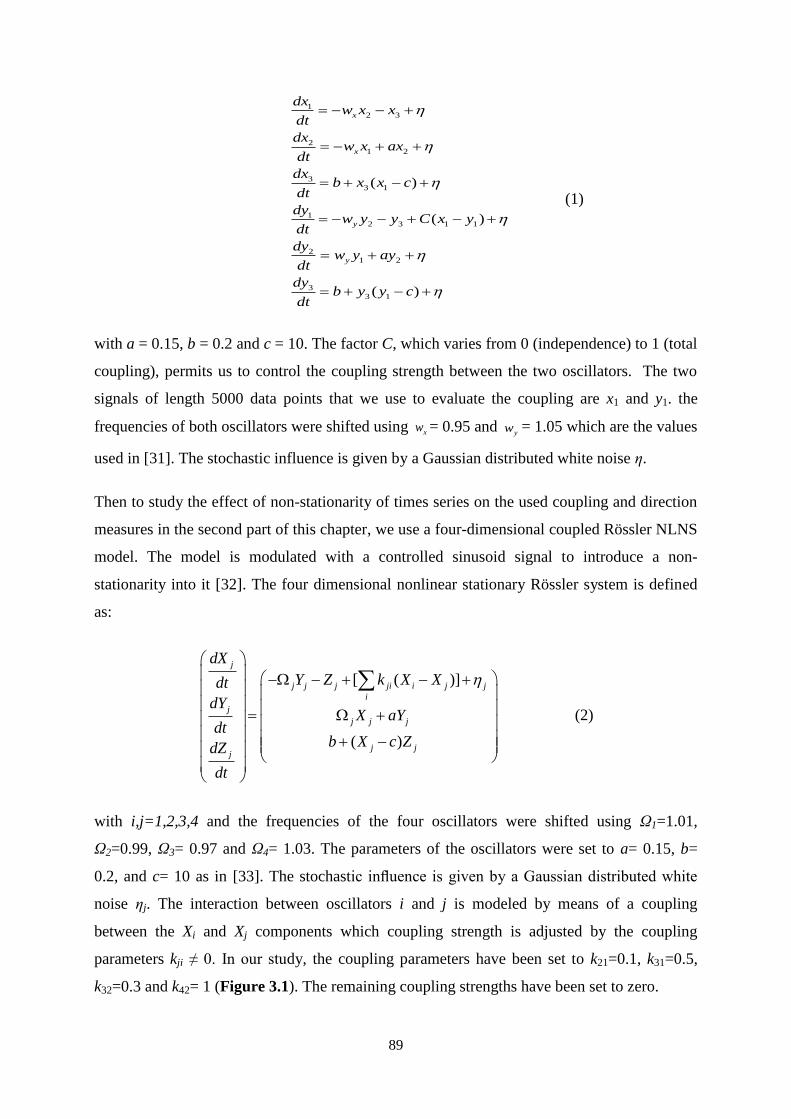
89

1

2 3

2

1 2

3

3 1

1

2 3 1 1

2

1 2

3

3 1

( )

( )

( )

x

x

y

y

dxw x x

dt

dxw x ax

dt

dxb x x c

dt

dyw y y C x y

dt

dyw y ay

dt

dyb y y c

dt

(1)

with a = 0.15, b = 0.2 and c = 10. The factor C, which varies from 0 (independence) to 1 (total

coupling), permits us to control the coupling strength between the two oscillators. The two

signals of length 5000 data points that we use to evaluate the coupling are x1 and y1. the

frequencies of both oscillators were shifted using xw = 0.95 and yw = 1.05 which are the values

used in [31]. The stochastic influence is given by a Gaussian distributed white noise η.

Then to study the effect of non-stationarity of times series on the used coupling and direction

measures in the second part of this chapter, we use a four-dimensional coupled Rössler NLNS

model. The model is modulated with a controlled sinusoid signal to introduce a non-

stationarity into it [32]. The four dimensional nonlinear stationary Rössler system is defined

as:

[ ( )]

( )

j

j j j ji i j j

i

j

j j j

j jj

dX

Y Z k X Xdt

dYX aY

dtb X c ZdZ

dt

(2)

with i,j=1,2,3,4 and the frequencies of the four oscillators were shifted using Ω1=1.01,

Ω2=0.99, Ω3= 0.97 and Ω4= 1.03. The parameters of the oscillators were set to a= 0.15, b=

0.2, and c= 10 as in [33]. The stochastic influence is given by a Gaussian distributed white

noise ηj. The interaction between oscillators i and j is modeled by means of a coupling

between the Xi and Xj components which coupling strength is adjusted by the coupling

parameters kji ≠ 0. In our study, the coupling parameters have been set to k21=0.1, k31=0.5,

k32=0.3 and k42= 1 (Figure 3.1). The remaining coupling strengths have been set to zero.

90

Figure 3.1: The map of direction using the reference coupling value.

The modulation of nonlinear stationary Rössler model to make it non-stationary is done by

using the sinusoidal signal S(n):

𝑆(𝑛) = 𝐴 sin 2 ∗ 𝜋 ∗ 𝑓0 ∗ 𝑛 𝑓𝑒 , (3)

where A=1, f0=0.1 Hz, n=0:4999 and fe=100 Hz. We modulate the output of each pilot

system by this sinusoid to obtain a non-linear non-stationary (NLNS) Rössler model.

This system has been simulated by using an Euler method with an integration step of 0.05 and

a sampling step of 0.1. We have generated 30 Monte Carlo instances of each signal with

length of 5000 data points. The time-series analysis techniques have been applied to the X-

components of the system.

3.2.1.2 Simulated signals from a uterus electrophysiological model

We used an electrophysiological model developed within a European project

(http://www.erasysbio.net/index.php?index=268). This multiscale model describes the

evolution of the uterine electrical activity, from its genesis at the cellular level, then to its

propagation at the myometrium level, and up to its projection through the volume conductor

tissues to the abdominal surface [23].

The electrical source is a volume current source density. For the volume conductor, we adopt

the description developed in [34]. The volume conductor is considered as made of parallel

interfaces separating the four different abdominal tissues, namely: the myometrium, where the

source is located at a given depth, the abdominal muscle, fat, and skin. Figure 3.2 presents a

representation of the model including tissue layers and the electrodes.

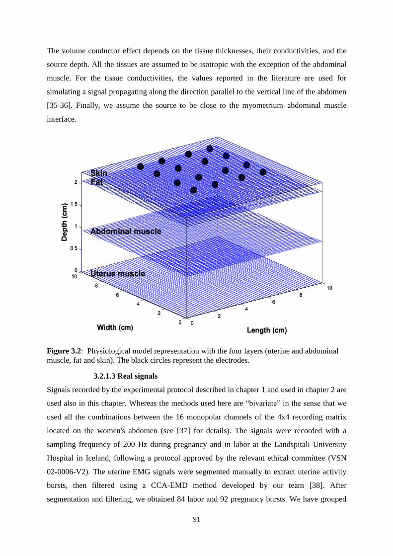
http://www.erasysbio.net/index.php?index=268

91

The volume conductor effect depends on the tissue thicknesses, their conductivities, and the

source depth. All the tissues are assumed to be isotropic with the exception of the abdominal

muscle. For the tissue conductivities, the values reported in the literature are used for

simulating a signal propagating along the direction parallel to the vertical line of the abdomen

[35-36]. Finally, we assume the source to be close to the myometrium–abdominal muscle

interface.

Figure 3.2: Physiological model representation with the four layers (uterine and abdominal

muscle, fat and skin). The black circles represent the electrodes.


Signals recorded by the experimental protocol described in chapter 1 and used in chapter 2 are

used also in this chapter. Whereas the methods used here are “bivariate” in the sense that we

used all the combinations between the 16 monopolar channels of the 4x4 recording matrix

located on the women's abdomen (see [37] for details). The signals were recorded with a

sampling frequency of 200 Hz during pregnancy and in labor at the Landspitali University

Hospital in Iceland, following a protocol approved by the relevant ethical committee (VSN

02-0006-V2). The uterine EMG signals were segmented manually to extract uterine activity

bursts, then filtered using a CCA-EMD method developed by our team [38]. After

segmentation and filtering, we obtained 84 labor and 92 pregnancy bursts. We have grouped

92

the segmented contractions in 7 groups of weeks before labor (WBL). Details for each group

are presented in Table 3.1. The analysis below was applied to these segmented uterine bursts.

3.2.2 Methods

3.2.2.1 Nonlinear correlation coefficient (h2)

The nonlinear correlation analysis is a nonparametric method used for evaluating the

dependency of a random process (signal Y) on another process (signal X), independently of

the type of relationship between the two processes.

The underlying idea is that if the value of X is considered as a function of the value of Y, the

value of Y given X can be predicted according to a nonlinear regression curve. The variance of

Y according to this regression curve is termed as the explained variance, since it is explained

(or predicted) by the knowledge of X. The unexplained variance is estimated by subtracting

the explained variance from the original one. The correlation ratio h2 describes the reduction

of variance of Y that can be obtained by predicting the Y values from those of X, according to

the regression curve, as h2

= (total variance − unexplained variance) / total variance.

In practice, to estimate the nonlinear correlation coefficient h2, a scatter plot of Y versus X is

studied. The values of X are subdivided into bins; for each bin we calculate the X value of the

midpoint Pi and the average value of Y, Qi, computed from the same bin interval. The

regression curve is approximated by connecting the resulting points (Pi, Qi) by straight line

segments. The nonlinear correlation coefficient between demeaned signals X and Y is then

calculated as follows (for more details see [39]):

22

2 1 1

| 2

1

N N

ik k

Y X N

k

Y k Y k f Xh

Y k

(4)

where N is the length of Y signal and f (Xi) is the linear piecewise approximation of the

nonlinear regression curve obtained using a continuous piecewise affine function. For

Table 3.1: Details on Database Group (WBL)

WBL 7 6 5 4 3 2 1 Labor

Number of women 1 2 2 4 6 4 5 5

Number of contractions 1 17 3 13 22 15 21 84

Mean Term 34 33 35 36 37 37 39 39

h2 standard deviation*10

-17

in Figure 3.6 0 0.9 0.99 3.2 2.3 1.1 2.5 7.9

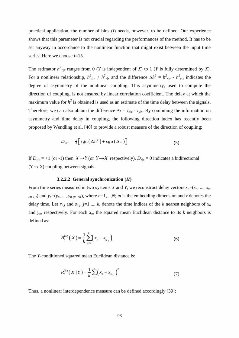
93

practical application, the number of bins (i) needs, however, to be defined. Our experience

shows that this parameter is not crucial regarding the performances of the method. It has to be

set anyway in accordance to the nonlinear function that might exist between the input time

series. Here we choose i=15.

The estimator h2

Y|X ranges from 0 (Y is independent of X) to 1 (Y is fully determined by X).

For a nonlinear relationship, h2

x|y ≠ h2

y|x and the difference ∆h2 = h

2x|y - h

2y|x indicates the

degree of asymmetry of the nonlinear coupling. This asymmetry, used to compute the

direction of coupling, is not ensured by linear correlation coefficient. The delay at which the

maximum value for h2 is obtained is used as an estimate of the time delay between the signals.

Therefore, we can also obtain the difference ∆τ = τx|y - τy|x. By combining the information on

asymmetry and time delay in coupling, the following direction index has recently been

proposed by Wendling et al. [40] to provide a robust measure of the direction of coupling:

21| 2

sgn sgnx y

D h (5)

If Dx|y = +1 (or -1) then X Y (or Y X respectively). Dx|y = 0 indicates a bidirectional

(Y ↔ X) coupling between signals.

3.2.2.2 General synchronization (H)

From time series measured in two systems X and Y, we reconstruct delay vectors xn=(xn, ..., xn-

(m-1)τ) and yn=(yn, ..., yn-(m-1)τ), where n=1,...,N; m is the embedding dimension and τ denotes the

delay time. Let rn,j and sn,j, j=1,..., k, denote the time indices of the k nearest neighbors of xn

and yn, respectively. For each xn, the squared mean Euclidean distance to its k neighbors is

defined as:

,

( )

1

1n j

kk

n n r

j

R X x xk

(6)

The Y-conditioned squared mean Euclidean distance is:

,

2

1

1|

n j

kk

n n s

j

R X Y x xk

(7)

Thus, a nonlinear interdependence measure can be defined accordingly [39]:

94

1

1| log

|

Nk n

kn n

R XH X Y

N R X Y

(8)

where Rn(X) is the average distance of a vector xn to all the other vectors. This measure is

close to zero if X and Y are independent, while it is positive if nearness in Y also implies

nearness in X for equal time partners. The nonlinear interdependence is an asymmetric

measure, in the sense that H(X|Y) ≠ H(Y|X) so H(X|Y) > H(Y|X), if X Y .

The phase space depends on two parameters, the time delay τ and the embedding dimension

m. We use the first local minimum of the average mutual information and the false nearest

neighbor algorithm to estimate the time delay (τ), and the minimal embedding dimension (m)

respectively. The estimated value of time delay and dimension were 10 and 6 respectively.

3.2.2.3 Granger causality (GC)

Granger argued that if X is influencing Y, then adding past values of the first variable to the

regression of the second one will improve its prediction performance, which can be assessed

by comparing the univariate and bivariate fitting of AR models to the signals [39]. The AR

model order is approximated to the Schwarz's Bayesian Criterion (SBC). Thus, for the

univariate case, one has:

1

1

,

p

xk x

k

p

yk y

k

x n a x n k u n

y n b y n k u n

(9)

where axk and byk are the model parameters, p the model order, and ux and uy are the

uncertainties or the residual noises associated with the model. Here, the prediction error, for a

given signal, depends only on its past values.

On the other hand, for bivariate AR modeling,

1 1

1 1

,

p p

xyk xyk xy

k k

p p

yxk yxk yx

k k

x n a x n k b y n k u n

y n a x n k b y n k u n

(10)

95

where the prediction error for each individual signal depends on the past values of both

signals. The prediction performance of both models can be assessed by the variances of the

prediction errors:

𝑉𝑋/𝑋− = 𝑉𝑎𝑟 𝑢𝑥 and 𝑉𝑌/𝑌− = 𝑉𝑎𝑟 𝑢𝑦 for the univariate AR model.

𝑉𝑋/𝑋−,𝑌− = 𝑉𝑎𝑟 𝑢𝑥𝑦 and 𝑉𝑌/𝑌−,𝑋− = 𝑉𝑎𝑟 𝑢𝑦𝑥 for the bivariate AR model.

Where Var(.) indicates the variance operator, and X|X_ and X|X_, Y_ indicate predicting X by

its past values alone and by past values of X and Y, respectively.

If 𝑉𝑋/𝑋−,𝑌− < 𝑉𝑋/𝑋− , then Y causes X in the sense of Granger causality. The Granger causality

of Y to X can be quantified as:

𝐺𝑌→𝑋 = ln 𝑉𝑋 /𝑋−

𝑉𝑋 /𝑋−,𝑌−

(11)

If 𝐺𝑌→𝑋 > 𝐺𝑋→𝑌 , then 𝑌 → 𝑋 and vice versa.

3.2.3 Bivariate piecewise stationary signal pre-segmentation

Several algorithms exist that can be used to segment a piecewise stationary signal. One such

algorithm was developed by Carré and Fernandez [41], used for univariate signal

segmentation. This algorithm starts by the decomposition of a signal into successive dyadic

partitions. The log-spectrum corresponding to each partition is computed and denoised by

undecimated wavelet transform if appropriate. A binary tree of the spectral distance between

two adjacent partitions is then formed. Then they search for the tree that minimizes the sum of

the spectral distances by Coifman-Wickerhauser algorithm.

Terrien et al. [28] used this technique to segment a pair of signals as pretreatment for

connectivity estimation. These methods have been used with success on monkey EHG signals

[28]. The segmentation was however based on the changes observed in only one of the signals

so transitions that may occur in the other signals are not taken into account.

To improve the method and to adapt it to the task of finding stationary parts of a pair of

signals, Terrien et al. [29] proposed to use the cross spectrum of the two signals instead of the

auto spectrum of only one channel, thus taking into account the statistical changes in both

channels at the same time. This preprocessing step has been proven to be useful for coupling

analysis. In the second part of this chapter, we adopt the approach developed by Terrien et al.

[29] since our methods are applied to bivariate signals.

96

3.2.4 From the methods to the direction maps

To estimate the coupling between two channel x and y, each method takes both signals x and y

as input. We took all the possible combinations of two channels among all the available

channels. We thus obtain n2 values of coupling for each method. These values were saved in a

matrix n x n (n is the number of channels and is equal to 2, 4 or 16 in case of bi-dimensional,

four dimensional synthetic signals or real signals respectively).

The above computation is done for each contraction (real EHG) and each Monte Carlo trial

(synthetic signals). If we have m contractions or m Monte Carlo trials, we obtain m x (n x n)

matrices of coupling values. Finally we compute the mean over the dimension m of the m x (n

x n) matrices to obtain just one n x n matrix for the m contractions or the m Monte Carlo

trials. These values in the final n x n matrix can be coded by color scale and represented in a

color map matrix (see Figure 3.5, Figure 3.7 and Figure 3.11). In Figure 3.6 and Figure 3.9,

we computed the mean of the final n x n matrix to obtain one value for each group.

We took from the final n x n coupling matrix, the value of coupling between x and y, and the

value between y and x. These values are used for the estimation of direction as mentioned

above in the methods description. Then we plot the map of direction as in Figure 3.5, Figure

3.7, Figure 3.8 and Figure 3.11.

When we use methods with bPSP, we do the same thing as above, but with an additional step,

the segmentation. We apply the methods to each segment of both signals (x and y), not to the

whole signals, then we take the mean over all segments and we continue as above.

3.3 Results

As we said in the introduction, this chapter is divided into two parts. We present first, the

results of the part that is dedicated to the comparison of methods using synthetic, simulated

and real data (Part 1). Then we present the results of the part that is dedicated to test their

sensitivity to some characteristics of the signal (nonstationarity, frequency band) or to signal

recording (bipolar or monopolar recording), (Part 2).

3.3.1 Part 1: Comparison of methods

3.3.1.1 Results on synthetic signals

Here we test the sensitivity of the methods to two signal aspects: varying coupling levels and

direction changes. To investigate the sensitivity of the methods to coupling changes we apply

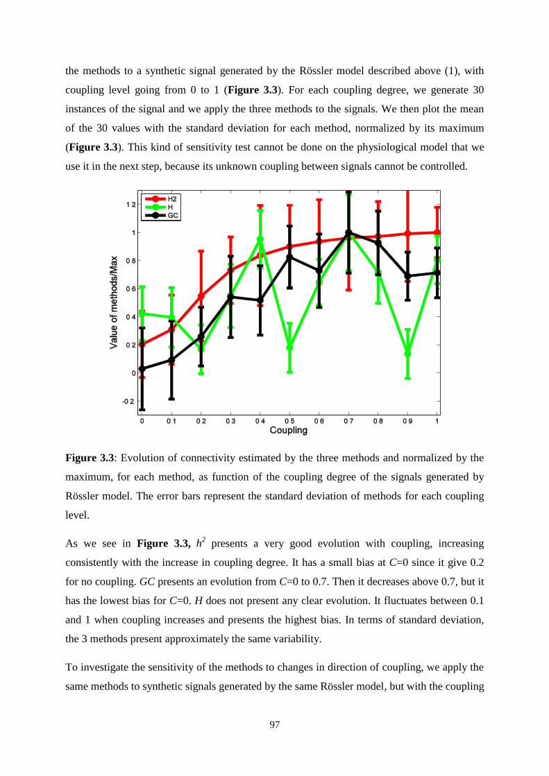
97

the methods to a synthetic signal generated by the Rössler model described above (1), with

coupling level going from 0 to 1 (Figure 3.3). For each coupling degree, we generate 30

instances of the signal and we apply the three methods to the signals. We then plot the mean

of the 30 values with the standard deviation for each method, normalized by its maximum

(Figure 3.3). This kind of sensitivity test cannot be done on the physiological model that we

use it in the next step, because its unknown coupling between signals cannot be controlled.

Figure 3.3: Evolution of connectivity estimated by the three methods and normalized by the

maximum, for each method, as function of the coupling degree of the signals generated by

Rössler model. The error bars represent the standard deviation of methods for each coupling

level.

As we see in Figure 3.3, h2 presents a very good evolution with coupling, increasing

consistently with the increase in coupling degree. It has a small bias at C=0 since it give 0.2

for no coupling. GC presents an evolution from C=0 to 0.7. Then it decreases above 0.7, but it

has the lowest bias for C=0. H does not present any clear evolution. It fluctuates between 0.1

and 1 when coupling increases and presents the highest bias. In terms of standard deviation,

the 3 methods present approximately the same variability.

To investigate the sensitivity of the methods to changes in direction of coupling, we apply the

same methods to synthetic signals generated by the same Rössler model, but with the coupling

98

degree fixed at 0.5 (Figure 3.4). The length of both generated signals is 6000 points. Initially,

the direction is from signal x1 to y1 for the whole signal duration. To create a direction change,

we cut the signals into three equal parts of 2000 points each. We keep the two extreme parts

of both signals unchanged and we swap their middle parts. The direction is then from x1 to y1

for the first and the third parts, and from y1 to x1 for the middle part, as indicated in Figure 3.4

(top) by the arrows and by the reference curve in Figure 3.4 (bottom). We then compute the

synchronization and the direction from x1 to y1 along the obtained signals. The results shown

in Figure 3.4 (middle) are the mean of 30 Monte-Carlo trials.

Figure 3.4: Sensitivity of methods to the change of direction between signals. Top: signal

generated by Rössler model after the change of direction; Middle: synchronization estimation;

Bottom: direction estimation. The blue curve is the reference curve.

We see in Figure 3.4 (middle) the superiority of h2 and GC over H, because the

synchronization measure given by h2 and GC in the middle part (2000-4000) is smaller than

the ones obtained for the extreme parts, which coincide with the reference curve. This is the

expected behavior since the coupling in the middle part is from y1 to x1 (due to the swap) and

the measure of synchronization is computed from x1 to y1. However, H gives an opposite

results which is erroneous and in contradiction with the underlying coupling. This erroneous

behavior is clearer in the plot of direction in Figure 3.4 (bottom), since 1 indicates a direction

from x1 to y1 and 0 the opposite direction. It is clear that h2 and GC give the right direction for

99

all signal parts while H gives the opposite of the true directions. This result is in agreement

with the previous evolution study.

According to both study results (coupling and direction) we can confirm that h2 is the best of

the 3 methods as it permits to evidence both coupling evolution and direction for the Rössler

synthetic model. We then move on testing h2 on the physiological model.

3.3.1.2 Results on signals from electrophysiological model

Figure 3.5 presents the test of h2

on simulated signals when applied to the physiological

model data. The model creates a propagating wave of excitation from a given initial site. This

results in a wave that has a known geometry. The model outputs a signal that would be

observed at the abdominal surface with the same electrode configuration as the one used when

measuring real signals (4x4 electrode grid).

We apply h2 to the signal obtained with a planar propagation in the uterus from left to right

under the electrode grid. We also apply h2

on a signal generated with a radial propagation,

with the origin close to the center of the electrode grid. After verification of their Gaussian

distributions, a threshold of m+2σ was applied to the results of the correlation matrix, where

m is the mean of the correlation matrix and σ its standard deviation. The threshold was applied

in order to remove insignificant coupling values among channels. The main purpose of this

processing was to increase the figure readability.

As we can see in the direction map in the case of planar propagation, Figure 3.5 (e), all the

arrows reveal the planar propagation of the action potential (left to right) illustrated in Figure

3.5 (a), but with a bi-directionality between most of the electrodes. The correlation among the

channels is distributed around the diagonal in the h2 matrix (Figure 3.5 (c)).

In the case of radial propagation, the direction of arrows in Figure 3.5 (f) is toward the center,

which reveals the radial propagation, but with some shifting to the left and to the top due to

the asymmetry of the center of the electrode grid with respect to the center of propagation.

Here, the correlation among channels shown in Figure 3.5 (d) is distributed to the whole

matrix. The results show that the underlying directionality and coupling is reflected by the

results obtained by computing h2 on the 4x4 matrix as well as on the directionality map. The

next step is to apply this technique to real signals expecting the observation of patterns in the

EHG that would reflect the underlying propagation of uterine activity.

100

(a) (b)

(c) (d)

(e) (f)

Figure 3.5: Results obtained with the physiological model of EHG propagation. Planar

propagation wave of action potential (a), radial propagation wave of action potential (b).

Quantity of information flow for planar propagation (c) and circular propagation (d).

Direction of information flow for planar propagation (e) and circular propagation (f) between

the 16 monopolar channels of uterine EMGs simulated by the physiological model when

using the h2 method.

Radial

101

3.3.1.3 Results on real signals

We investigate in this section the coupling evolution measured by h2 (Figure 3.6) with respect

to decreasing term before delivery (WBL). We also calculate the matrix of correlation using

h2 (Figure 3.7 (a-c-e-g)), and the direction map (Figure 3.7 (b-d-f-h)) between the 16

monopolar channels of real signals, recorded at 3 WBL, 2 WBL, 1 WBL and during labor, in

order to visually monitor the changes in the correlation matrix and the direction map along

term. We observe also the difference between EHG connectivity of pregnancy and labor

contractions.

h2 was applied to real uterine EMGs recorded on several women during different times of

gestation. h2 was applied to all the possible combinations of the 16 channels, for each

contraction in each WBL. We plot in Figure 3.6 the mean of the resultant coupling matrix

over all the contractions for each WBL. A Kruskal-Wallis statistical test was applied to the

results (Table 3.2). The most significant differences represented in bold in Table 3.2 (p<0.01)

between all gestational groups for h2 are presented graphically in Figure 3.6.

It is clear from Figure 3.6 that there is no monotonic evolution from 7 WBL to labor. The

means of each WBL data are associated to extremely low standard deviations (red bars),

which are also presented in Table 3.1. h2 increases between 7 and 4 WBL, decreases between

2 WBL and labor, and exhibits a rupture at 3WBL.

Figure 3.6: Evolution of connectivity estimated by h2 as a function of weeks before labor

(WBL), with its standard deviation (red).

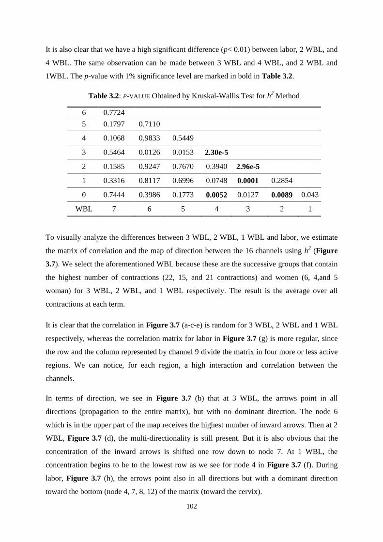
102

It is also clear that we have a high significant difference (p< 0.01) between labor, 2 WBL, and

4 WBL. The same observation can be made between 3 WBL and 4 WBL, and 2 WBL and

1WBL. The p-value with 1% significance level are marked in bold in Table 3.2.

To visually analyze the differences between 3 WBL, 2 WBL, 1 WBL and labor, we estimate

the matrix of correlation and the map of direction between the 16 channels using h2 (Figure

3.7). We select the aforementioned WBL because these are the successive groups that contain

the highest number of contractions (22, 15, and 21 contractions) and women (6, 4,and 5

woman) for 3 WBL, 2 WBL, and 1 WBL respectively. The result is the average over all

contractions at each term.

It is clear that the correlation in Figure 3.7 (a-c-e) is random for 3 WBL, 2 WBL and 1 WBL

respectively, whereas the correlation matrix for labor in Figure 3.7 (g) is more regular, since

the row and the column represented by channel 9 divide the matrix in four more or less active

regions. We can notice, for each region, a high interaction and correlation between the

channels.

In terms of direction, we see in Figure 3.7 (b) that at 3 WBL, the arrows point in all

directions (propagation to the entire matrix), but with no dominant direction. The node 6

which is in the upper part of the map receives the highest number of inward arrows. Then at 2

WBL, Figure 3.7 (d), the multi-directionality is still present. But it is also obvious that the

concentration of the inward arrows is shifted one row down to node 7. At 1 WBL, the

concentration begins to be to the lowest row as we see for node 4 in Figure 3.7 (f). During

labor, Figure 3.7 (h), the arrows point also in all directions but with a dominant direction

toward the bottom (node 4, 7, 8, 12) of the matrix (toward the cervix).

Table 3.2: P-VALUE Obtained by Kruskal-Wallis Test for h2 Method

6 0.7724

5 0.1797 0.7110

4 0.1068 0.9833 0.5449

3 0.5464 0.0126 0.0153 2.30e-5

2 0.1585 0.9247 0.7670 0.3940 2.96e-5

1 0.3316 0.8117 0.6996 0.0748 0.0001 0.2854

0 0.7444 0.3986 0.1773 0.0052 0.0127 0.0089 0.043

WBL 7 6 5 4 3 2 1

103

(a) (b)

(c) (d)

(e) (f)

(g) (h)

Figure 3.7: Quantity (a-c-e-g) and direction (b-d-f-h) of information flow recorded at 3 WBL

(a-b), 2 WBL (c-d), 1 WBL (e-f) and Labor (g-h), between the 16 monopolar channels of

EHG by using the h2 method. Each coupling graph is normalized by its maximum.

3 WBL

2 WBL

1 WBL

Labor

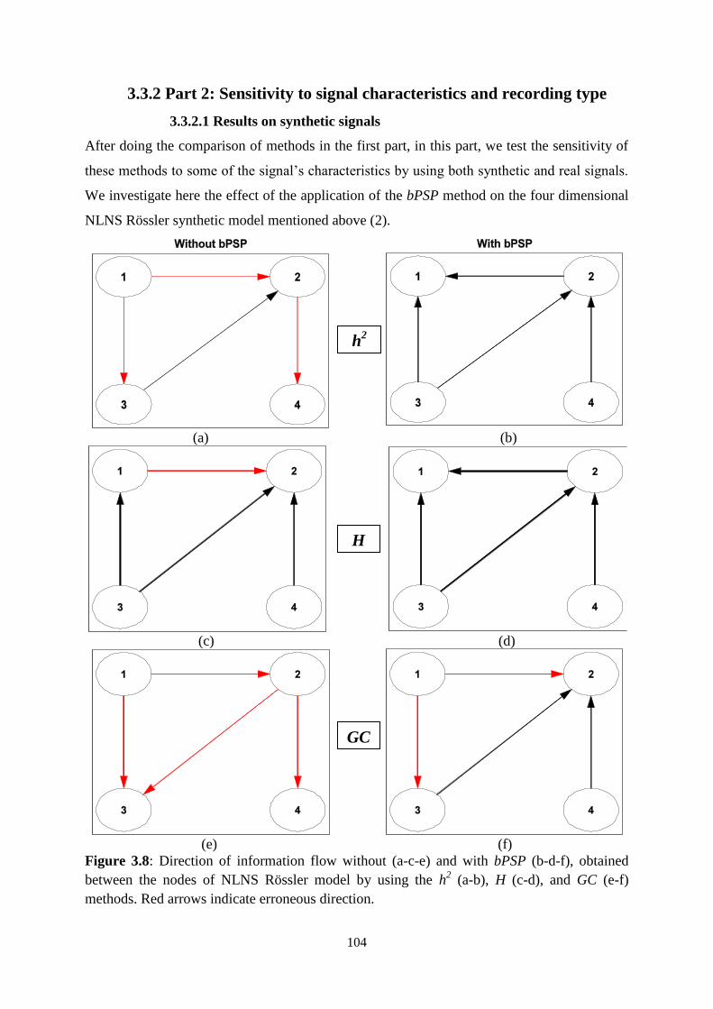
104

3.3.2 Part 2: Sensitivity to signal characteristics and recording type

3.3.2.1 Results on synthetic signals

After doing the comparison of methods in the first part, in this part, we test the sensitivity of

these methods to some of the signal‟s characteristics by using both synthetic and real signals.

We investigate here the effect of the application of the bPSP method on the four dimensional

NLNS Rössler synthetic model mentioned above (2).

(a) (b)

(c) (d)

(e) (f)

Figure 3.8: Direction of information flow without (a-c-e) and with bPSP (b-d-f), obtained

between the nodes of NLNS Rössler model by using the h2 (a-b), H (c-d), and GC (e-f)

methods. Red arrows indicate erroneous direction.

h2

H

GC

105

We plot in Figure 3.8 the map of coupling directions (node with arrows) between all the

combination of simulated time series in two cases, with and without bPSP, for h2, H, and GC

Figure 3.8 (a-b), Figure 3.8 (c-d), and Figure 3.8 (e-f) respectively. The arrows indicate the

coupling directions, black arrows indicate the detection of a correct direction and red arrows

indicates a wrong direction. We see in Figure 3.8 (a-b) that h2 applied without bPSP has 3 out

of 4 direction errors (red), whereas its bPSP application rectifies all the errors by correctly

detecting all four directions. It is clear from Figure 3.8 (c-d) that H works better than h2 when

it is applied without bPSP since it has just 1 out of 4 direction error. This one error is

corrected by using bPSP before H. Figure 3.8 (e-f) show that GC is the worst method since it

has 4 out of 4 direction errors when applied without bPSP. Using bPSP, the GC direction

error rate improves a little and reaches 2 out of 4. According to results on synthetic signals we

can confirm that the bPSP approach improves the detection of correct coupling direction. We

therefore apply our methods to real EHG signals using the with bPSP approach as we estimate

that the above results conclusively show that this generally helps with the nonstationarity

issue.

3.3.2.2 Results on real signals

We investigate in this section the ability of the methods to differentiate between pregnancy

and labor contraction groups. We apply our methods with bPSP to all the available bipolar

and monopolar EHG bursts (Figure 3.9 (a-b)). Then we apply the same methods to the same

signals after bPSP, but with filtering to isolate the lower EHG frequency band (FWL) as

additional pretreatment (Figure 3.9 (c-d)). Figure 3.9 presents the mean and standard

deviations of the method results applied for each kind of measurement type and each group of

EHG signals (labor and pregnancy).

In Figure 3.9 (a-b), GC gives higher coupling for labor than for pregnancy in both cases

(monopolar and bipolar). But we obtain higher standard deviation in the monopolar case than

in the bipolar case. h2 gives higher coupling values for labor than for pregnancy, only in the

monopolar case, with low standard deviation in both cases. The H method shows a higher

coupling for pregnancy than for the labor group with relatively low standard deviations in

both monopolar and bipolar cases. All methods give lower coupling in the bipolar (Figure 3.9

(a)) than the monopolar (Figure 3.9 (b)) case for both groups.

It is not surprising to obtain such results for GC since this linear method cannot deal with the

non linear non stationary characteristics of the EHG signal, as shown by the work on synthetic

106

signals (Figure 3.8 (e-f)). On the other hand we are surprised by the results obtained when

using h2. Indeed h

2 did not demonstrate a significant difference between labor and pregnancy,

even if it increases slightly from pregnancy to labor. H gave the most unexpected result, since

its value decreases from pregnancy to labor.

(a) (b)

(c) (d)

Figure 3.9: Estimated coupling difference between pregnancy and labor contractions

estimated by h2, H, and GC applied with bPSP using bipolar (a) and monopolar (b) uterine

EMG signals. And with bPSP and filtering together using bipolar (c) and monopolar (d)

uterine EMG signals; method/P (method/L) means results obtained for a given method on

pregnancy (respectively Labor) group.

A well-known hypothesis is that the propagation of EHG is more related to the low frequency

components (FWL) of the EHG signal [42]. Therefore, in an attempt to improve the results,

we try to filter the EHG to isolate the low frequency band (0.1Hz-0.3Hz) by using a

Butterworth filter, as a preprocessing step, before applying our methods with bPSP. The

results obtained are shown for bipolar (Figure 3.9 (c)) and monopolar (Figure 3.9 (d))

signals.

107

In general, the estimated coupling values increase after filtering when compared to results in

Figure 3.9 (a-b). We note that the filtering reversed the result for GC for monopolar signals

(Figure 3.9 (d)), since its value now decreases from pregnancy to labor. For the h2 method,

the difference between pregnancy and labor increases when compared to Figure 3.9 (a-b). To

test the statistical significance of the obtained differences, we apply a simple two tails student

t-test for h2 results with and without filtering, but with bPSP, in bipolar and monopolar cases.

It is clear from Table 3.3 that filtering makes pregnancy/labor difference more significant, for

both monopolar and bipolar cases (**

: p<1%). It is also clear that the use of monopolar

measurement type is better than the bipolar one, since h2 yields better significant difference

both with and without filtering in the monopolar case.

H always decreases from pregnancy to labor even after filtering, in both the bipolar and

monopolar cases. We know that H computes the synchronization in a phase space (detailed in

chapter 2), which is highly influenced by the nonlinearity (chaotic characteristic) and the

complexity of the signals. We know also that the complexity and nonlinearity of the EHG

signals increase when going from pregnancy to labor [43]. To explain the unexpected results

given by H, we then go back to synthetic signals. We apply the three methods on coupled

signals generated using a bivariate version of the same NLNS Rössler model, but by changing

the dissipative parameter c that controls the model chaotic characteristics.

Figure 3.10 presents the evolution of all the methods with changing chaoticity degree c from

2 to 10. We notice that H decreases when the chaoticity of signals increases, opposite to h2

behavior as shown in Figure 3.10. GC does not show any monotonic evolution. This result

could explain why H method always decreases from pregnancy associated to non-chaotic

EHG (almost linear, non complex), to labor associated to chaotic EHG (nonlinear, complex),

even when using bPSP and filtering.

Table 3.3: P-VALUE Obtained by Student t-test for h2 Method

Without filtering With Filtering

Method Bipolar Monopolar Bipolar Monopolar

h2 0.9796 0.1873 0.0068

** 9.7105e

-05**

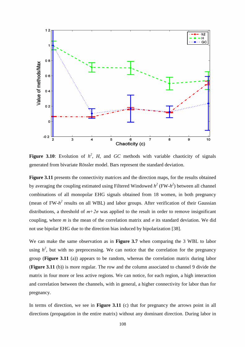
108

Figure 3.10: Evolution of h2, H, and GC methods with variable chaoticity of signals

generated from bivariate Rössler model. Bars represent the standard deviation.

Figure 3.11 presents the connectivity matrices and the direction maps, for the results obtained

by averaging the coupling estimated using Filtered Windowed h2 (FW-h

2) between all channel

combinations of all monopolar EHG signals obtained from 18 women, in both pregnancy

(mean of FW-h2 results on all WBL) and labor groups. After verification of their Gaussian

distributions, a threshold of m+2σ was applied to the result in order to remove insignificant

coupling, where m is the mean of the correlation matrix and σ its standard deviation. We did

not use bipolar EHG due to the direction bias induced by bipolarization [38].

We can make the same observation as in Figure 3.7 when comparing the 3 WBL to labor

using h2, but with no preprocessing. We can notice that the correlation for the pregnancy

group (Figure 3.11 (a)) appears to be random, whereas the correlation matrix during labor

(Figure 3.11 (b)) is more regular. The row and the column associated to channel 9 divide the

matrix in four more or less active regions. We can notice, for each region, a high interaction

and correlation between the channels, with in general, a higher connectivity for labor than for

pregnancy.

In terms of direction, we see in Figure 3.11 (c) that for pregnancy the arrows point in all

directions (propagation in the entire matrix) without any dominant direction. During labor in

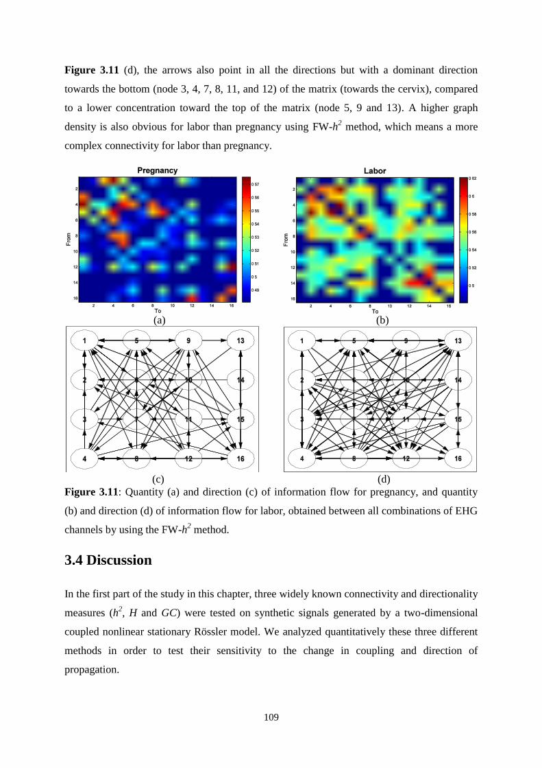
109

Figure 3.11 (d), the arrows also point in all the directions but with a dominant direction

towards the bottom (node 3, 4, 7, 8, 11, and 12) of the matrix (towards the cervix), compared

to a lower concentration toward the top of the matrix (node 5, 9 and 13). A higher graph

density is also obvious for labor than pregnancy using FW-h2 method, which means a more

complex connectivity for labor than pregnancy.

(a) (b)

(c) (d)

Figure 3.11: Quantity (a) and direction (c) of information flow for pregnancy, and quantity

(b) and direction (d) of information flow for labor, obtained between all combinations of EHG

channels by using the FW-h2 method.

3.4 Discussion

In the first part of the study in this chapter, three widely known connectivity and directionality

measures (h2, H and GC) were tested on synthetic signals generated by a two-dimensional

coupled nonlinear stationary Rössler model. We analyzed quantitatively these three different

methods in order to test their sensitivity to the change in coupling and direction of

propagation.

110

These measures were first applied to the synthetic Rössler model with increasing coupling to

test their abilities to follow the coupling variation. h2 was the best method among the three to

detect and follow the coupling. However, GC shows poor evolution for low coupling values

and then decreases after C = 0.7. H did demonstrated no evolution with increasing coupling

value. Our results confirm those obtained by Ansari et al. [44] who found that h2 is the best

method for evaluating coupling variation among all the studied methods. However Ansari

measured only the strength of coupling whereas, in our study we also estimated the ability of

the methods to correctly indicate the direction of coupling. The performance of GC is

expected since its linear characteristics cannot deal with the nonlinearity of signal model. At

the opposite, the performance of H method was not expected. They may be due to H high

dependency on the chaotic characteristics of the model, as shown in the results of Part 2. All

methods presented similar variability regarding their standard deviation.

The h2 and GC methods were able to estimate the correlation between the signals x1 and y1

(Figure 3.4 (top)) with respect to the direction change (Figure 3.4 (middle)), as well as to

indicate the correct direction (Figure 3.4 (bottom)). The H method, however, failed to detect

the correct direction and indicated the opposite of the true direction, when the methods were

applied to the same model with an inversion of the coupling direction of a part of the signal,

with a given level of coupling (section 2.3.1.1).

To summarize our findings on the stationary bivariate Rössler synthetic signals, h2 was found

to be sensitive to both coupling and direction variation whereas GC was found to be sensitive

to direction changes and slightly sensitive to coupling changes. H was insensitive to both

coupling and direction changes. We therefore selected h2 as the most robust and appropriate

method to be applied to simulated signals generated by the physiological model of EHG

developed by our team.

The new physiological model is supposed to simulate real signals better than the Rössler

model. However the coupling degree between its output signals cannot be controlled as for

Rössler model. In case of a simulated planar propagation, h2

evidenced the correct direction

related to the signal propagation, but with a bi-directionality between adjacent channels. This

is due to the simultaneous presence of two propagating waves under the electrode matrix. In

the circular propagation case, the direction of arrows is towards the center with some shifting

to the left and the top. This concentration to the center is related to the presence of 2 AP

waves inducing that the previous action potential should explain the next one generated at the

111

center (Figure 3.5 (b)). The shifting comes from the edge effects. Indeed, the action potential

encounters the left and the top edges before the right and the bottom ones (Figure 3.5 (b)).

Hence the previous action potential explains the top and the left of the new action potential

before the bottom and the right one. This phenomenon is expressed by a shifting in the

direction map.

The synchronization between channels is restricted to the diagonal in the planar case because

the propagation is only longitudinal. Thus the connection is only in one direction (between

electrodes on the same line). In the case of circular propagation, the synchronization is

propagated through the whole matrix. In this case, the electrodes are recruited by the waves in

all the directions at the same time; so the synchronization simultaneously spreads to the whole

matrix. The conclusion is that h2 permitted to evidence properly the main characteristics of the

signals propagated by this physiological model.

h2 was then applied to a dataset of uterine EMG signals. We first studied the evolution of

coupling with the term of gestation (WBL). h2 presented some increase at the beginning, then

lost this trend after 3 WBL. This is to be expected since the closer we are to labor, the closer

the characteristics of pregnancy contractions will be to labor contractions, and the more

difficult the differentiation between them will be. Results of a Kruskal-Wallis statistical test

applied to the h2 results between the different WBL and labor, evidenced a significant

difference only between 1, 2, 3, 4 WBL and labor. This could be due to the inter-individual

variability of the women included in this study (Figure 3.12).

Figure 3.12 show the variability in the behavior of h2 applied individually to each of the 6

women measured longitudinally that is at different pregnancy terms. Therefore when we take

the mean of all contractions measured on all women at each WBL we cannot find the

expected increase due to the huge inter-individual variability evidenced Figure 3.12.

112

Figure 3.12: Evolution of h2 applied on the 6 women, who were measured longitudinally on

more than one term, in function of WBL.

Finally, we monitor the pregnancy by following the changes in the matrix of synchronization

and in the map of direction for signals recorded at 3 WBL, 2 WBL, 1 WBL and during labor

by using h2. Results demonstrated an increase in synchronization and a more regular pattern

of synchronization (4 highly correlated regions), as well as a higher concentration of direction

toward the cervix, when going from pregnancy to labor. This is in agreement to our previous

results [10, 17, 45].

To sum up, the main findings of the first part of this study are the following: (i) the H method

is insensitive to varying signal coupling and varying coupling direction, whereas GC is

sensitive to direction variation and slightly sensitive to coupling variation; (ii) h2 reveals the

right coupling and direction when used with the physiological model; (iii) h2 did not display a

significant increase related to term; (iv) the evolution of h2 with WBL is highly affected by

the inter-individual variability; (v) in general there is an increase in the regularity of coupling

and the direction is more focused toward the cervix when going from pregnancy to labor.

Our next aim in the Part 2 of this study was to improve the performance of the methods used

by compensating for the nonstationarity of the signals (such as computing methods in

113

predefined segments), and by focusing on FWL component, which is supposed to be more

related to the propagation of EHG signals.

Therefore, the same connectivity measures (h2, H and GC) as used in the first part, were tested

in the second part on synthetic signals generated this time by a four-dimensional coupled

NLNS Rössler model. We analyzed quantitatively these three different methods in order to

test the effect of nonstationarity on direction estimation, and the improvement induced by

bPSP approach effect on direction estimation for these NLNS signals.

The general synchronization (H) method was shown to be the most efficient method without

using bPSP among the 3 methods since it has the lowest direction error (1 out of 4), Figure

3.8 (c). h2 has an intermediate performance since it has 3 out of 4 direction errors. GC is the

worst method since it did not detect any of the correct direction (4 out of 4 direction errors).

The bPSP approach corrected the errors in the estimations of directions for h2 and H thus

giving same performance for both methods, whereas GC still have a 2 out of 4 direction

errors, even after bPSP.

On real signals Hassan et al. [45] used h2 to process bipolar signals recorded on one

pregnancy contraction and one labor contraction, and on one women measured longitudinally

at 3 terms. They obtained a good pregnancy/labor differentiation with an increase from

pregnancy to labor. When we apply our three methods including h2 on our bigger database, h

2

and GC did not demonstrate any monotonic increasing behavior from pregnancy to labor. H

methods decreased when going from pregnancy to labor, as shown in Figure 3.13.

114

Figure 3.13: Evolution of methods with WBL on our bigger database without any pre-

processing.

Terrien et al. applied the bPSP segmentation algorithm on monkey EHG signals. They also

investigated the filtering of the monkey signals into higher frequency band (FWH), but their

aim was to see the effect on h2 results inside the contractions not to study any pregnancy/labor

differentiation [29]. However, Terrien et al. investigated in another study the effect of filtering

into low frequency band (FWL) on the pregnancy/labor classification rate by using h2.

Whereas in this study they use the filtering solely without bPSP and on bipolar signals, not on

monopolar signals as in our case [11]. Their results are in agreement with our results since,

after filtering, they found that the significance of pregnancy/labor differentiation increases.

Finally, Terrien et al. [46] presented a way to correct the bias of h2 by using surrogates. This

approach worked very well on monkey EHG signals. Using surrogates is however very time

consuming in terms of computation. Furthermore, using surrogates did not improve our

results (evolution with WBL) on human EHG signals (Figure 3.14).

115

Figure 3.14: Evolution of h2 without (green) and with (blue) correction in function of WBL.

Therefore, we propose a Filtering-Windowing approach as a suitable method for this signal,

since the EHG is a non-stationary signal with propagation mainly related to low frequencies.

These two characteristics should be taken into account by bPSP and FWL filtering

respectively. We apply our approach on bipolar as well as monopolar signals, since, as we

know, the way of measuring signals affects the detection and the quality of these signals and

consequently the results of the applied methods [30]. Indeed, the bipolarization of signals

induces some bias for the direction computation.

As we see in Figure 3.9, the bPSP approach did not improve the results of GC as it still gives

non-significant difference between pregnancy and labor due to the high variance (especially

for the monopolar case). The results of h2 was improved slightly by bPSP alone, since it

increased instead of decreasing (without bPSP), when going from pregnancy to labor. But the

difference was non-significant and small especially in bipolar case. H was not improved by

bPSP since it still decreased in both monopolar and bipolar cases. These results are in

agreement with the ones obtained on synthetic signals.

The second step of our approach was filtering signals between 0.1 and 0.3 Hz (low frequency)

associated with the segmentation of signals. This step makes the difference between

pregnancy and labor more significant (see Figure 3.9 and Table 3.3). We suppose that this is

116

due to the fact that filtering reducing the EHG frequency content to FWL band, we focus on

the more propagated part of this signal [42]. Furthermore, when we checked the PSD of our

EHG signals, we noticed that their frequency content is strongly affected by the women‟s

weight or body mass index. For example Figure 3.15, since the fat in the abdomen for a

heavy woman has a strong low pass filtering effect (Figure 3.15 (right)), for a thin women the

EHG frequency band is larger (Figure 3.15 (left)).

Figure 3.15: Channel-frequency plot for one contraction of thin women (65.5 Kg) at 38 week

of gestation (left), and for another contraction of heavy women (111 Kg) at 40 week of

gestation with weight = 111 Kg (right).

This fat filtering effect is bypassed by reducing and thus homogenizing the bands for all the

EHG measurements (FWL filtering), and making the measure independent of the woman‟s

weight. This filtering thus increased the significance difference between pregnancy and labor

groups.

The use of monopolar recordings is better than bipolar ones according to Table 3.3, since the

significance difference between pregnancy and labor group with and without filtering is better

for monopolar than bipolar recordings.

H always decreased in all cases from pregnancy to labor. This could be due to the fact that H

is highly influenced by chaoticity (nonlinearity and complexity) of the signals. Using

simulation, we demonstrated (Figure 3.10) that H decreases when chaoticity increases

opposite to h2. This evolution of EHG from almost linear (pregnancy) to complex (labor)

characteristics has been evidenced on real signals. Indeed, uterus goes from an almost

117

deterministic state during pregnancy to a chaotic (nonlinear and complex) state during labor

as shown in [43].

Finally we compared the matrix of connectivity and the map of direction for signals recorded

during pregnancy and labor by using FW-h2. Results show an increase in coupling and a more

regular pattern of synchronization between the 16 unipolar nonlinear, complexsignals (4

highly correlated regions) as well as a higher concentration of direction towards the cervix for

labor than for pregnancy which is coherent with our previous studies. We identify also a

higher graph density (number of arrows) for labor than pregnancy, which represents a more

complex pattern in labor than in pregnancy which agrees well with results in [43]. This

increase in coupling and synchronization during labor induces fast contractions of the whole

uterus. The concentration of coupling direction towards the cervix may help in pushing the

baby out.

3.5 Conclusion and perspectives

The above results permit us to conclude that the h2 method is a good candidate for measuring

EHG coupling and direction as it is able to correctly detect them for synthetic and simulated

EHG signals. Due to subject variability, h2 did not show a monotonic increasing behavior

along with WBL. But when we perform a longitudinal study from 3 WBL to labor, the

coupling matrix show more regular pattern for labor than for pregnancy. An interesting

evolution happens to the direction when going from pregnancy to labor: it becomes more

highly concentrated toward the cervix as labor progresses.

We can also conclude that in our case (application to EHG) two preprocessing steps (FW-h2)

permit to increase significantly h2 performance. When using FW-h

2, labor group demonstrates

higher coupling than pregnancy, which is in agreement with the literature. Also, when using

FW-h2, the density of the direction map is higher for the labor than for the pregnancy group.

The H method performance is highly influenced by the nonlinearity of EHG signals and

therefore it requires further investigation. Monopolar recordings are better than bipolar one.

We think that these findings are likely to be valuable to help us to solve the problem of the

preterm labor detection.

A promising next step of the work would be to extract parameters from the connectivity

graphs by using a graph theory based approach (considering the electrodes as nodes and the

118

connectivity lines as edges of the graph). Different parameters such as density of graphs and

ingoing and outgoing edges for each node, can be used to quantify the uterine connectivity,

and thus help us to get new parameters to discriminate between pregnancy and labor

contractions, which is the ultimate goal of our project.

References

[1] M. Rosenblum, and J. Kurths, “Analysing synchronization phenomena from bivariate data by

means of the Hilbert transform”. in Nonlinear analysis of physiological data. Springer Berlin:

Heidelberg, 1998: pp. 91-99.

[2] J. Sun, X. Hong, and S. Tong, “Phase synchronization analysis of EEG signals: an evaluation

based on surrogate tests,” IEEE Trans. Biomed. Eng., vol. 59, no. 8, pp. 2254-2263, Aug. 2012.

[3] K. Majumdar, “Constraining minimum-norm inverse by phase synchronization and signal

power of the scalp EEG channels,” IEEE Trans. Biomed. Eng., vol. 56, no. 4, pp. 1228-1235,

Apr. 2009.

[4] A. Porta, V. Bari, F. Badilini, E. Tobaldini, T. Gnecchi-Ruscone, and N. Montano, “Frequency

domain assessment of the coupling strength between ventricular repolarization duration and

heart period during graded head-up tilt,” Journal of Electrocardiology, vol. 44, no. 6, pp. 662-

668, Nov.-Dec. 2011.

[5] E. Oczeretko, J. Swiatecka, A. Kitlas, T. Laudanski, and P. Pierzynski, “Visualization of

synchronization of the uterine contraction signals: running cross-correlation and wavelet

running cross-correlation methods,” Medical engineering & physics, vol. 28, no. 1, pp. 75,

2006.

[6] A. Diab, M. Hassan, J. Laforet, B. Karlsson, and C. Marque, “Estimation of Coupling and

Directionality between Signals Applied to Physiological Uterine EMG Model and Real EHG

Signals,” in Proc. XIIIMediterranean Conference on Medical and Biological Engineering and

Computing 2013, Sevilla, Spain, Sep. 2014, pp. 718-721.

[7] A. Diab, M. Hassan, B. Karlsson, and C. Marque, “Effect of decimation on the classification

rate of nonlinear analysis methods applied to uterine EMG signals,” IRBM, vol. 34, no. 4-5, pp.

326-329, Oct. 2013.

[8] B. Karlsson, M. Hassan, and C. Marque, “Windowed multivariate autoregressive model

improving classification of labor vs. pregnancy contractions,” in Proc. IEEE Eng. Med. Biol.

Soc. Conf. 2013, Osaka, Japan, Jul. 2013, pp. 7444-7447.

[9] P. F. Panter, “Modulation, noise, and spectral analysis: applied to information transmission,”

New York: McGraw-Hill, 1965, pp. 767.




119

[11] J. Terrien, T. Steingrimsdottir, C. Marque, and B. Karlsson, “Synchronization between EMG at

Different Uterine Locations Investigated Using Time-Frequency Ridge Reconstruction:

Comparison of Pregnancy and Labor Contractions,” EURASIP J. Adv. Signal Process., vol.

2010, pp. 1-10, Jun. 2010.

[12] C. Alvarez, and S. Reynolds, “A better understanding of uterine contractility through

simultaneous recording with an internal and a seven channel external method,” Surgery,

gynecology & obstetrics, vol. 91, no. 6, pp. 641-650, Dec. 1950.

[13] T. Y. Euliano, D. Marossero, M. T. Nguyen, N. R. Euliano, J. Principe, and R. K. Edwards,

“Spatiotemporal electrohysterography patterns in normal and arrested labor,” Amer. J. Obstet.

Gynecol., vol. 200, no. 1, pp. 54 e1–54 e7, Jan. 2009.

[14] W.J. Lammers, H. Mirghani, B. Stephen, S. Dhanasekaran, A. Wahab, M.A.H. Al Sultan, and F.

Abazer, “Patterns of electrical propagation in the intact pregnant guinea pig uterus,” Am. J.

Physiol. Regul. Integr. Comp. Physiol., vol. 294, no. 3, pp. R919-28, Mar. 2008.



745-61, Jun. 2009.

[16] E. Mikkelsen, P. Johansen, A. Fuglsang-Frederiksen, and N. Uldbjerg, “O452 propagation

direction and velocity of uterine EMG signals during labor,” International Journal of

Gynecology & Obstetrics, vol. 119, pp. S421, Oct. 2012.

[17] A. Diab, M. Hassan, S. Boudaoud, C. Marque, and B. Karlsson, “Nonlinear estimation of

coupling and directionality between signals: Application to uterine EMG propagation,” in Proc.

IEEE Eng. Med. Biol. Soc. Conf. 2013, Osaka, Japan, Jul. 2013, pp. 4366-4369.

[18] E. Mikkelsen, P. Johansen, A. Fuglsang‐Frederiksen, and N. Uldbjerg, “Electrohysterography of


Scandinavica, vol. 92, no. 9, pp. 1070-1078, Sept. 2013.



pp. e86775, Jan. 2014.

[20] J. Pijn, and F. Lopes Da Silva, “Propagation of electrical activity: nonlinear associations and

time delays between EEG signals,” in Basic Mechanisms of the EEG. Birkhäuser Boston, 1993,

pp. 41-61.

[21] J. Arnhold, P. Grassberger, K. Lehnertz, and C.E. Elger, “A robust method for detecting

interdependences: application to intracranially recorded EEG,” Phys D: Nonlin Phen, vol. 134,

no. 4, pp. 419-30, Dec. 1999.

[22] C. W. J. Granger, “Investigating causal relations by econometric models and cross-spectral

methods,” Econometrica: Journal of the Econometric Society, vol.37, no. 3, pp. 424-438, Jul.

1969.

120

[23] J. Laforet, C. Rabotti, J. Terrien, M. Mischi, C. Marque, “Toward a Multiscale Model of the


2011.

[24] C. Marque and J. Duchêne, “Human abdominal EHG processing for uterine contraction

monitoring,” in Applied Sensors. Boston, MA: Butterworth, 1989, pp. 187–226.


different sites investigated using wavelet analysis: Comparison of pregnancy and labor

contractions,” EURASIP J. Adv. Signal Process., vol. 2010, no. 17, pp. 1–10, Feb. 2010.

[26] J. G. Planes, J. P. Morucci, H. Grandjean, and R. Favretto, “External recording and processing

of fast electrical activity of the uterus in human parturition,” Med. Biol. Eng. Comput., vol. 22,

no. 6, pp. 585–591, Nov. 1984.


R. E. Garfield, “Noninvasive uterine electromyography for prediction of preterm delivery,”

Amer. J. Obstet. Gynecol., vol. 204, no. 3, pp. 228–238, Mar. 2011.

[28] J. Terrien, M. Hassan, C. Marque, and B. Karlsson, “Use of piecewise stationary segmentation

as a pre-treatment for synchronization measures,” in Proc. IEEE Eng. Med. Biol. Soc. Conf.

2008, Vancouver, BC, Aug. 2008, pp. 2661-2664.

[29] J. Terrien, G. Germain, C. Marque, and B. Karlsson, “Bivariate piecewise stationary

segmentation; improved pre-treatment for synchronization measures used on non-stationary

biological signals,” Medical engineering & physics, vol. 35, no. 8, pp. 1188-96, Aug. 2013.

[30] J. Alberola-Rubio, G. Prats-Boluda, Y. Ye-Lina, J. Valerob, A. Peralesb, and J. Garcia-Casado,

“Comparison of non-invasive electrohysterographic recording techniques for monitoring uterine

dynamics,” Medical engineering & physics, vol. 35, no. 12, pp. 1736-1743, Dec. 2013.

[31] M. G. Rosenblum, A. S. Pikovsky, and J. Kurths, “Phase synchronization of chaotic

oscillators,” Phys Rev Lett, vol. 76, no. 11, pp. 1804-1807, Mar. 1996.

[32] P. Borgnat, P. Flandrin, P. Honeine, and C. Richard, “Testing stationarity with surrogates: A

time-frequency approach,” IEEE Trans. Sig. Process., vol. 58, no. 7, pp. 3459-3470, Jul. 2010.

[33] M. Winterhalder, B. Schelter, W. Hesse, K. Schwab, L. Leistritz, D. Klan, R. Bauer, J.

Timmer, and H. Witte, “Comparison of linear signal processing techniques to infer directed

interactions in multivariate neural systems,” Signal Process., vol. 85, no. 11, pp. 2137-60, Nov.

2005.

[34] C. Rabotti, M. Mischi, L. Beulen, S. Oei, and J. Bergmans, “Modeling and identification of the

electrohysterographic volume conductor by highdensity electrodes,” IEEE Trans. Biomed. Eng.,

vol. 57, no. 3, pp. 519–527, Mar. 2010.

[35] L. Mesin and R. Merletti, “Distribution of electrical stimulation current in a planar multilayer

anisotropic tissue,” IEEE Trans. Biomed. Eng., vol. 55, no. 2, pp. 660–670, Feb. 2008.

121

[36] S. Gabriel, R. Lau, and C. Gabriel, “The dielectric properties of biological tissues: II.

Measurements in the frequency range 10 Hz to 20 GHz,” Phys. Med. Biol., vol. 41, pp. 2251–

2269, Nov. 1996.



11th Mediterranean Conference on Medical and Biological Engineering and Computing, 2007,

Ljubljana, Slovenia, 2007, pp. 139-143.




[39] E. Pereda, R.Q. Quiroga, and J. Bhattacharya, “Nonlinear multivariate analysis of

neurophysiological signals,” Progress in Neurobiology, vol. 77, no. 1-2, pp. 1-37, Sep.-Oct.

2005.

[40] F. Wendling, F. Bartolomei, J. J. Bellanger, and P. Chauvel, “Interpretation of

interdependencies in epileptic signals using a macroscopic physiological model of the EEG,”

Clin Neurophysiol, vol. 112, no. 7, pp. 1201-1218, Jul. 2001.

[41] P. Carré, and C. Fernandez, “Research of stationary partitions in nonstationary processes by

measurement of spectral distance with the help of nondyadic Malvar's decomposition,” in IEEE-

SP International Symposium on Time-Frequency and Time-Scale Analysis, Pittsburgh, PA,

USA, Oct. 1998, pp. 429 - 432.


electromyography: a critical review,” Am J Obstet Gynecol, vol. 169, no. 6, pp. 1636-53, Dec.

1993.

[43] M. Hassan, J. Terrien, B. Karlsson, and C. Marque, “Comparison between approximate

entropy, correntropy and time reversibility: Application to uterine electromyogram signals,”

Medical engineering & physics, vol. 33, no. 8, pp. 980-986, oct. 2011.

[44] K. Ansari-Asl, L. Senhadji, J. J. Bellanger, and F. Wendling, “Quantitative evaluation of linear

and nonlinear methods characterizing interdependencies between brain signals,” Physical

review E, vol. 74, no. 3, pp. 031916, Sept. 2006.

[45] M. Hassan, J. Terrien, B. Karlsson, and C. Marque, “Spatial analysis of uterine EMG signals:

evidence of increased in synchronization with term,” in Proc. IEEE Eng. Med. Biol. Soc. Conf.

2009, Minneapolis, USA, Sep. 2009, pp. 6296-6299.

[46] J. Terrien, M. Hassan, G. Germain, C. Marque, and B. Karlsson, “Nonlinearity testing in the

case of non Gaussian surrogates, applied to improving analysis of synchronicity in uterine

contraction,” Proc. IEEE Eng. Med. Biol. Soc. Conf., Minneapolis, USA, Sep. 2009, pp. 3477-

80.

122

Chapter 4: Uterine EMG source localization

One of the primary concerns in electrophysiology is the non-invasive localization of the origin

of the measured uterine EMG (electrohysterogram, EHG) activity. Methods for localization of

unknown sources from their effect far away are termed inverse methods and the solutions that

they provide inverse solutions. We tackle in this chapter the problem of uterine source

localization. Source localization has been widely applied to EEG [1-4], MEG [5-7], but to our

knowledge it has never been applied to EHG signal. The work presented in this chapter is

therefore the first attempt to localize uterine EMG sources. The methods which were

developed to solve the inverse problem are divided into two main families, mainly the non

parametric (over-determined) and parametric (under-determined) methods [8]. For non-

parametric methods, we find various techniques including minimum norm estimates and their

generalizations (LORETA, sLORETA, VARETA, S-MAP, ST-MAP, Backus-Gilbert,

LAURA, Shrinking LORETA FOCUSS (SLF), SSLOFO and ALF). For the parametric

methods, there are the beamforming techniques, BESA, the subspace techniques such as

MUSIC and methods derived from it, the FINES, simulated annealing and computational

intelligence algorithms [8]. The main difference between the two is whether a fixed number of

dipoles is a priori assumed (parametric) or not (non-parametric).

4.1 Introduction

In our application to EHG, we do not have a priori information on source number, strength

and location. Therefore we focused on the non-parametric methods. We begin by testing the

basic method of this family, which is the minimum norm estimate (MNE) method.

Source estimation is a general tool for analyzing spatiotemporal dynamics of organs or

system. Uterine EMG stand out among the different non-invasive techniques that can be used

to study the functionality of the uterus, due to its high temporal resolution. It could permit to

observe the dynamics of uterine contractile activity on a time-scale of milliseconds, reflecting

synchronous activity of cells within the uterus muscle. EHG can therefore provide a dynamic

characterization of uterus activity which is not possible with other direct and indirect

modalities presented in chapter 1. Therefore, in this work, we implemented source estimation

tool for the uterus electrical activity, using the FieldTrip open-source software [9]. Simulated

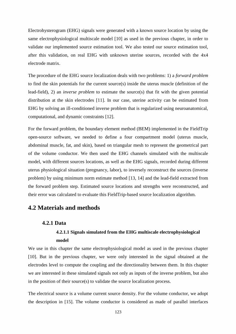
123

Electrohysterogram (EHG) signals were generated with a known source location by using the

same electrophysiological multiscale model [10] as used in the previous chapter, in order to

validate our implemented source estimation tool. We also tested our source estimation tool,

after this validation, on real EHG with unknown uterine sources, recorded with the 4x4

electrode matrix.

The procedure of the EHG source localization deals with two problems: 1) a forward problem

to find the skin potentials for the current source(s) inside the uterus muscle (definition of the

lead-field), 2) an inverse problem to estimate the source(s) that fit with the given potential

distribution at the skin electrodes [11]. In our case, uterine activity can be estimated from

EHG by solving an ill-conditioned inverse problem that is regularized using neuroanatomical,

computational, and dynamic constraints [12].

For the forward problem, the boundary element method (BEM) implemented in the FieldTrip

open-source software, we needed to define a four compartment model (uterus muscle,

abdominal muscle, fat, and skin), based on triangular mesh to represent the geometrical part

of the volume conductor. We then used the EHG channels simulated with the multiscale

model, with different sources locations, as well as the EHG signals, recorded during different

uterus physiological situation (pregnancy, labor), to inversely reconstruct the sources (inverse

problem) by using minimum norm estimate method [13, 14] and the lead-field extracted from

the forward problem step. Estimated source locations and strengths were reconstructed, and

their error was calculated to evaluate this FieldTrip-based source localization algorithm.

4.2 Materials and methods

4.2.1 Data

4.2.1.1 Signals simulated from the EHG multiscale electrophysiological

model

We use in this chapter the same electrophysiological model as used in the previous chapter

[10]. But in the previous chapter, we were only interested in the signal obtained at the

electrodes level to compute the coupling and the directionality between them. In this chapter

we are interested in these simulated signals not only as inputs of the inverse problem, but also

in the position of their source(s) to validate the source localization process.

The electrical source is a volume current source density. For the volume conductor, we adopt

the description in [15]. The volume conductor is considered as made of parallel interfaces

124

separating the four different abdominal tissues, namely: the myometrium (where the source is

located) with conductivity = 0.2 S/m and depth = 0; the abdominal muscle with conductivity

0.2 S/m and 0.4 S/m respectively in the X and Y directions, and thickness = 0.936 cm; fat

with conductivity = 0.04 S/m and thickness = 1.132 cm; and skin with conductivity = 0.5 S/m

and thickness = 0.2 cm. To limit computation time we only simulate a square of 10x10 cm

divided into 204x204 computational elements, of the uterus muscle and the above abdomen

conductor volume is simulated. This area is supposed to be near the median axis of the uterus,

where the surfaces are supposed to be more or less flat and parallel.

Figure 4.1 presents a representation of the model including the 4 tissue layers, the electrodes

placement, and an example for placement of one source at the center of the uterine muscle

layer. The volume conductor effect depends on the tissue thicknesses, their conductivities, and

the source depth. All the tissues are assumed to be isotropic with the exception of the

abdominal muscle. Finally, we assume the source to be close to the myometrium–abdominal

muscle interface.

Figure 4.1: The uterus EHG model representation of the volume conductor for the

physiological multiscale model, with the four layers (uterine and abdominal muscle, fat and

skin). The 16 black disks above the skin layer represent the electrodes. The black disk in the

uterus muscle layer represents an example for a source at the center of the uterine muscle.


As in the previous chapter we use signals recorded by the experimental protocol described in

chapter 1. The signals are recorded using 16 monopolar channels of a 4x4 recording matrix

125

located on the women's abdomen (see [16] for details), and filtered using the CCA-EMD

method [17]. We tested our source localization tool on pregnancy and labor signals to see

what might be the difference between these two physiological situations in terms of uterine

dynamic. Understanding what happens to this uterine dynamic when going from pregnancy to

labor has been a question of great interest for a long time.

4.2.2 Methods

4.2.2.1 Forward problem (BEM)

In order to locate the source for the specific activity seen on the abdomen skin, we first have

to solve the forward problem [18]. This problem is to define the rules of the signal

propagation from the source to the recorded site (here the abdominal skin) [18]. This problem

involves calculating the electric potentials generated by known current sources for a given

anatomical model.

Forward modeling is done in our case based on a volume-conduction model that describes the

geometrical and electrical properties of the tissue in the abdomen above the uterus. The

volume conduction often requires a geometrical description of tissue boundaries in the

abdomen [19]. The uterus model used in this chapter for EHG analysis assumes that the

abdomen above the uterus consists of a set of meshes, triangulated surfaces in 3D-space,

representing the uterine muscle, abdomen muscle, fat, and skin. If the conductivities within

each of these regions are isotropic and constant, the electric potentials can be expressed in

terms of surface integrals. The forward EHG problems can then be solved numerically using a

boundary-element method (BEM) [20-22]. We used in this step the same geometrical and

electrical definitions that the ones used for the physiological multiscale model (illustrated

figure 4.1). The mesh is done with a precision of 51x51 elements.

BEM calculates the potentials/fields of the non-intersecting homogeneous regions bounded by

the uterine muscle, abdominal muscle, fat, and skin surface boundaries, each one having a

conductivity (σ) values of 0.2, 0.2 and 0.4, 0.04 and 0.33 S/m respectively.

To solve the forward problem we should compute the lead field matrix represented by the

following equation:

𝐿𝑖𝑗 =1

4𝜋𝜎

𝑟∅𝑖 − 𝑟𝑗 𝑗

𝑟∅𝑖 − 𝑟𝑗 𝑗 3

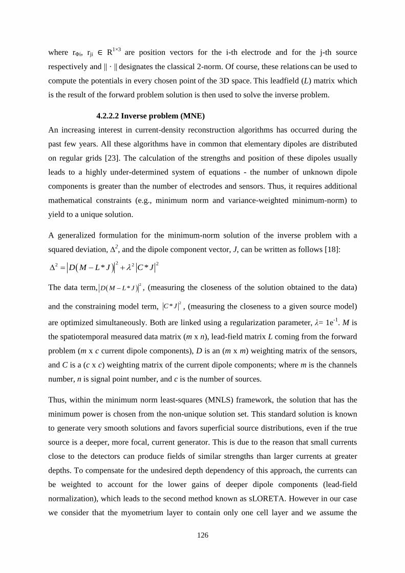
126

where rΦi, rji ∈ R1×3

are position vectors for the i-th electrode and for the j-th source

respectively and || · || designates the classical 2-norm. Of course, these relations

can be used to

compute the potentials in every chosen point of the 3D space.

This leadfield (L) matrix which

is the result of the forward problem solution is then used to solve the inverse problem.

4.2.2.2 Inverse problem (MNE)

An increasing interest in current-density reconstruction algorithms has occurred during the

past few years. All these algorithms have in common that elementary dipoles are distributed

on regular grids [23]. The calculation of the strengths and position of these dipoles usually

leads to a highly under-determined system of equations - the number of unknown dipole

components is greater than the number of electrodes and sensors. Thus, it requires additional

mathematical constraints (e.g., minimum norm and variance-weighted minimum-norm) to

yield to a unique solution.

A generalized formulation for the minimum-norm solution of the inverse problem with a

squared deviation, ∆2, and the dipole component vector, J, can be written as follows [18]:

The data term, , (measuring the closeness of the solution obtained to the data)

and the constraining model term, , (measuring the closeness to a given source model)

are optimized simultaneously. Both are linked using a regularization parameter, λ= 1e-1

. M is

the spatiotemporal measured data matrix (m x n), lead-field matrix L coming from the forward

problem (m x c current dipole components), D is an (m x m) weighting matrix of the sensors,

and C is a (c x c) weighting matrix of the current dipole components; where m is the channels

number, n is signal point number, and c is the number of sources.

Thus, within the minimum norm least-squares (MNLS) framework, the solution that has the

minimum power is chosen from the non-unique solution set. This standard solution is known

to generate very smooth solutions and favors superficial source distributions, even if the true

source is a deeper, more focal, current generator. This is due to the reason that small currents

close to the detectors can produce fields of similar strengths than larger currents at greater

depths. To compensate for the undesired depth dependency of this approach, the currents can

be weighted to account for the lower gains of deeper dipole components (lead-field

normalization), which leads to the second method known as sLORETA. However in our case

we consider that the myometrium layer to contain only one cell layer and we assume the

2 22 2* *D M L J C J

2

*D M L J

2*C J

127

source to be close to the myometrium–abdominal muscle interface. Therefore we are not

interested in the source depth.

4.3 Results

The same strategy used in the previous chapter is also used here. We will validate our

methods on simulated signals in different cases using the electrophysiological model before

applying the methods to real signals. In our application to real signal we localize the sources

of one pregnancy contraction and one labor contraction recorded on the same woman, to see

how the uterine dynamic evolves from pregnancy to labor. In all the figures below we plot the

obtained localization on the mesh of the myometrial muscle.

4.3.1 Results on simulated signals

We have simulated three cases of source generation: i) two synchronous sources with circle

propagation waveform; ii) two asynchronous sources with circle propagation waveform; iii) a

longitudinal bar of sources that propagates longitudinally. This “plane wave” type

propagation corresponds to a source similar to the ones in case i), but viewed from a point

distant from the source. The results of sources localization are presented Figure 4.2(a-b) for

the first case (synchronous sources that begin at the same time), Figure 4.2(c-d) for the

second case (asynchronous sources which have a delay between their onset), and Figure

4.2(e-f) for the third case (bar of sources that propagate longitudinally). Each picture of

Figure 4.2 represents the source localization result for a single instant of the signal generated

in each case. Subfigures (a), (c) and (e) represent the original sources generated by the

multiscale physiological model; subfigures (b), (d) and (f) represent the corresponding

sources estimated by our algorithm.

It is clear from Figure 4.2 that our implemented forward/inverse algorithm is able to localize

the given sources in all cases. We can see in Figure 4.2(a) and (b) approximately the same

wave front shapes, after the collision of the two circle waves generated by the two

synchronous sources. After the collision of the original wave fronts, the resulting wave fronts

propagate to the corners with no source, Figure 4.2(b).

Figure 4.2(c) and (d) also present similar shapes. In Figure 4.2(d) a yellow circle shape is

first generated by the source propagating from the bottom left corner, represented by the blue

disk. The second source generated at the top right corner (Figure 4.2(c)), represented by the

magenta disk, is also well localized with some error in its position (Figure 4.2(d)).

128

Simulated two synchronous sources Estimated two synchronous sources

Simulated two asynchronous sources Estimated two asynchronous sources

Simulated bar of sources Estimated bar of sources

Figure 4.2: Simulation of two synchronous (a), asynchronous (c) and vertical bars (e)

sources, and their estimated localization and propagation (b), (d) and (f) respectively, for a

single instant. The colored disks in (b) and (d) and the red bar in (f) represent the position of

the original source.

b) a)

c) d)

e) f)

129

In Figure 4.2(e) and (f), our method was also able to detect the waves fronts generated at the

left of the mesh and their propagation.

However, the estimated wave fronts are always thicker than the actual simulated source ones

introduced into the physiological multiscale model. We can also notice a precision error in the

localization, as well as a smaller power for the estimated wave front than for the initial

simulated sources.

We thus computed the localisation error for one time instant of the synchronous case and for

two time instants of the asynchronous sources presented in Figure 4.3. We computed the

absolute and the relative (relative to the reference postion) errors on both, x and y, dimensions

of the mesh, as well as the euclidian distance between the simulated and the estimated sources

(Table 4.1). The position of the estimated source(s) is the one(s) of the maximum value(s) for

each instant.

As we see in all figures the localization is done with some error. We should notice here that

the dimension of one element in the original mesh is 0.049 cm whereas in the decimated mesh

it is 0.196 cm. For the case of synchronous sources (Figure 4.3(a-b)), the absolute error on x

for the estimated source 1 is equal to the absolute error on y for the estimated source 2 and

vice versa. The relative error of source 2 is smaller than the relative error of source 1. Both

estimated sources have the same distances from the original sources, which is equal to 1.2 cm

(Table 4.1).

In the case of asynchronous sources the absolute error is the same for the estimated sources 1

(Figure 4.3(c-d)) and 2 (Figure 4.3(e-f)). As in the case of synchronous source, the relative

error of the estimated source 2 is smaller than the estimated error of source 1 for the case of

asynchronous sources. Both estimated sources have the same distances from the original

sources, which is equal to 0.9 cm (Table 4.1).

We can see also from Table 4.1 that the localization is better for the asynchronous cases

(which are more realistic) then for the synchronous case, since the absolute and relative errors

in asynchronous cases are smaller than for the synchronous case. The distance between the

original and estimated sources is also smaller for asynchronous cases than for the synchronous

case.

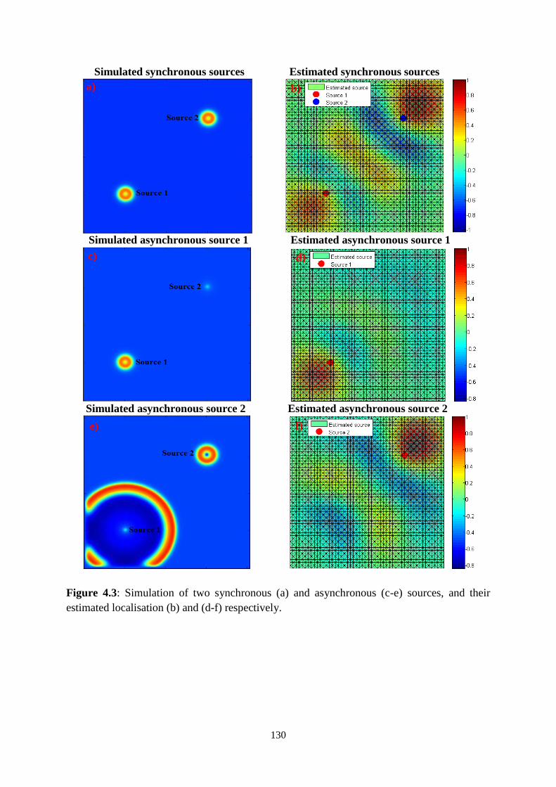
130

Simulated synchronous sources Estimated synchronous sources

Simulated asynchronous source 1 Estimated asynchronous source 1

Simulated asynchronous source 2 Estimated asynchronous source 2

Figure 4.3: Simulation of two synchronous (a) and asynchronous (c-e) sources, and their

estimated localisation (b) and (d-f) respectively.

a) b)

c) d)

e) f)

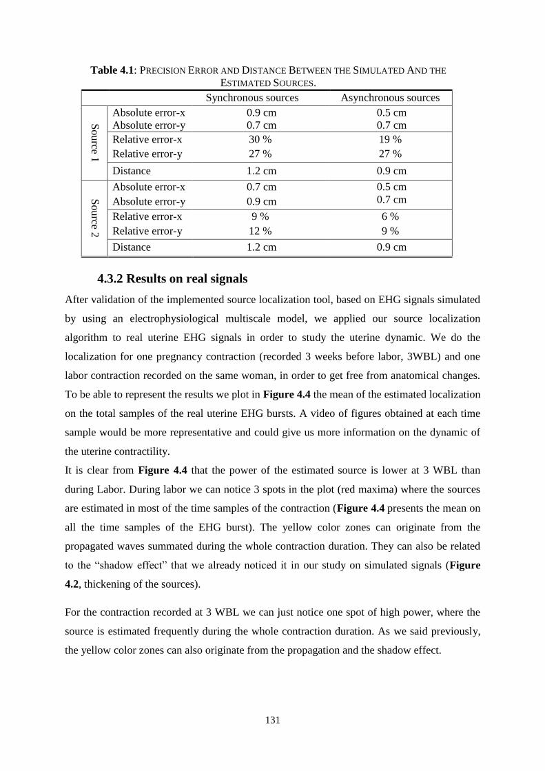
131

4.3.2 Results on real signals

After validation of the implemented source localization tool, based on EHG signals simulated

by using an electrophysiological multiscale model, we applied our source localization

algorithm to real uterine EHG signals in order to study the uterine dynamic. We do the

localization for one pregnancy contraction (recorded 3 weeks before labor, 3WBL) and one

labor contraction recorded on the same woman, in order to get free from anatomical changes.

To be able to represent the results we plot in Figure 4.4 the mean of the estimated localization

on the total samples of the real uterine EHG bursts. A video of figures obtained at each time

sample would be more representative and could give us more information on the dynamic of

the uterine contractility.

It is clear from Figure 4.4 that the power of the estimated source is lower at 3 WBL than

during Labor. During labor we can notice 3 spots in the plot (red maxima) where the sources

are estimated in most of the time samples of the contraction (Figure 4.4 presents the mean on

all the time samples of the EHG burst). The yellow color zones can originate from the

propagated waves summated during the whole contraction duration. They can also be related

to the “shadow effect” that we already noticed it in our study on simulated signals (Figure

4.2, thickening of the sources).

For the contraction recorded at 3 WBL we can just notice one spot of high power, where the

source is estimated frequently during the whole contraction duration. As we said previously,

the yellow color zones can also originate from the propagation and the shadow effect.

Table 4.1: PRECISION ERROR AND DISTANCE BETWEEN THE SIMULATED AND THE

ESTIMATED SOURCES.

Synchronous sources Asynchronous sources

Source 1

Absolute error-x

Absolute error-y

0.9 cm

0.7 cm

0.5 cm

0.7 cm

Relative error-x

Relative error-y

30 %

27 %

19 %

27 %

Distance 1.2 cm 0.9 cm

Source 2

Absolute error-x

Absolute error-y

0.7 cm

0.9 cm

0.5 cm

0.7 cm

Relative error-x

Relative error-y

9 %

12 %

6 %

9 %

Distance 1.2 cm 0.9 cm

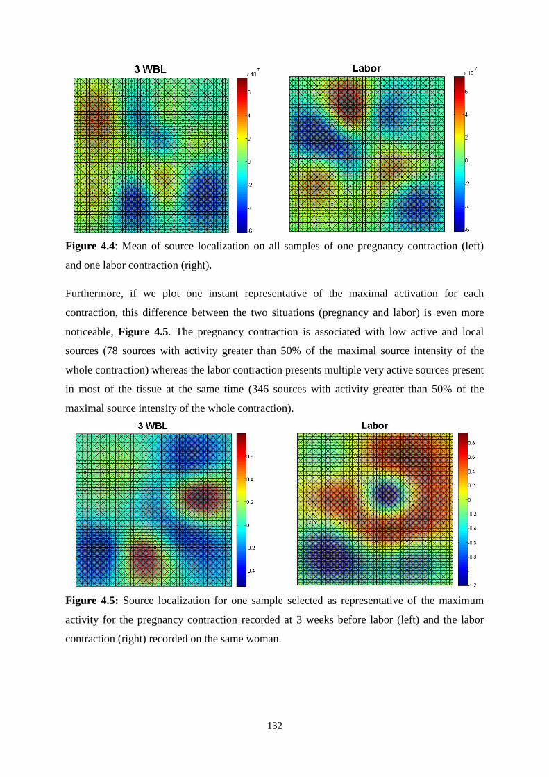
132

Figure 4.4: Mean of source localization on all samples of one pregnancy contraction (left)

and one labor contraction (right).

Furthermore, if we plot one instant representative of the maximal activation for each

contraction, this difference between the two situations (pregnancy and labor) is even more

noticeable, Figure 4.5. The pregnancy contraction is associated with low active and local

sources (78 sources with activity greater than 50% of the maximal source intensity of the

whole contraction) whereas the labor contraction presents multiple very active sources present

in most of the tissue at the same time (346 sources with activity greater than 50% of the

maximal source intensity of the whole contraction).

Figure 4.5: Source localization for one sample selected as representative of the maximum

activity for the pregnancy contraction recorded at 3 weeks before labor (left) and the labor

contraction (right) recorded on the same woman.

133

Figure 4.6: Evolution of the number of active elements along the contraction duration for a

contraction recorded at 3 weeks before labor (a) and one labor contraction (b) recorded on the

same woman.

We then compute, for each time sample, the number of elements which activity is greater than

50% of the maximal source intensity, identified for each whole contraction. The results

(Figure 4.6) present an indicator of the contraction dynamic. We can see that the number of

active elements is always greater and more frequent (6414 identified time sample where the

elements activity is greater than 50% of the maximal source intensity) for the labor

contraction than for the pregnancy one (1674 identified time sample where the elements

activity is greater than 50% of the maximal source intensity), indicating a more synchronous

activity of the whole uterine tissue investigated by our electrode grid.

b)

a)

134

4.4 Discussion

In this work, we solved the first step of source localization, the forward problem, by using the

BEM method for a 10x10 cm uterus model with four tissue layers. Simulated and real signals

were then used as inputs of the inverse problem by using MNE method. The study on

simulated signals presented three cases: two synchronous sources, two asynchronous sources,

and a bar of sources. Results show that MNE is able to localize the sources and to detect their

propagation with some minor precision error. We computed the localization error for the first

two cases and we found that source 2 is better localized than source 1. Furthermore, the more

realistic case, asynchronous sources, gave better precision than the synchronous one. We

think that most of the localization error comes from the down sampling of the mesh (to limit

memory usage), since the mesh is decimated by factor of 4. Therefore the localization error

could perhaps better be termed “resolution” as it is closely related to the sampling of the space

under investigation. Also for all the cases of simulated signals, the wave front is detected

thicker than its actually size. This could be due to the high velocity of wave propagation in the

model and to the well known „cone shape‟ of the volume seen by the electrodes. It looks like a

shadow following the wave front.

After validation of the forward and inverse problem on simulated signals, we applied these

methods to a pregnancy and a labor contractions, in order to attempt to localize the origin of

the contractions and to detect its propagation. This information would permit us to better

understand the functioning of uterus during pregnancy and labor, which may eventually help

us in preterm labor prediction. We found that the sources intensity of labor contraction is

higher than for pregnancy one. We clearly evidenced three sources for the labor contraction

whereas pregnancy contraction presented only one source. This appears to be logical since as

we know labor contractions are more efficient then pregnancy ones. We expect labor

contractions to be more global (propagating fast to the whole uterus) whereas pregnancy

contraction remains more or less localized (smaller propagation).

But the localized sources did not demonstrate any “propagation like” behavior. Indeed, the

dynamic of the sources evidenced for each time sample of each contraction appeared more

like a blowing or an erupting one than a propagated one. This could be in agreement with the

hypothesis proposed by Young [24] who stated that the mechanism of global organ-level

communication is probably not via action potential propagation, but may be via a

135

hydrodynamic-stretch activation mechanism, including a coupling between the electrical and

the mechanical properties of the uterine organ.

However in the application on real signals we were limited by the geometry of the model

(cube containing parallel plane surfaces), which is far from a real uterus. Also we are limited

by the electrodes configuration, since the signals in our database are measured by 16

electrodes arranged in a plan matrix placed on a small part of the abdomen, near the vertical

median axis of the uterus. These 16 electrodes are spatially localized and do not cover the

whole uterus. So they do not provide us with a global image of the uterus. In this case some

regions of interest may be missed if they are far from the recording site. In this case, the

electrodes are collinear and the localization problem is undetermined, regardless of the

number of available signals. The dipole component orthogonal to the plane determined by the

electrode and the origin of the dipole cannot be seen by any of the sensors [25]. These issues

can affect our results and contribute to the source estimation error.

In all cases however, the intensity of the identified sources remained very small for real

signal. This problem could come from the characteristic of the MNLS method itself

(minimum norm least-squares) that searches for the solution that presents the minimum

power. We could solve this drawback by using another method, such as sLOTERA, that gives

also information on the depth of the source.

4.5 Conclusion and perspectives

A first preliminary study on EHG source localization problem was presented in this chapter.

A validation of forward and inverse methods was done on simulated signals in different cases.

Then we applied these methods on real uterine EHG bursts, corresponding to contractions

recorded during pregnancy and labor. The methods were able to identify the sources injected

in the model for the simulated signals, with some error, related to the mesh decimation. On

real EHG signals, the methods gave logical results that fit with the well-known hypothesis in

the literature, which says that during labor the contraction is efficient and propagated to the

whole uterus, whereas during pregnancy, the contraction is inefficient and local.

In a future work, we will study the effect of varying the velocity and of the regularization

parameter λ on the results. We will also attempt to use the whole mesh in order to see the

effect of mesh resolution on the localization error. We will also compare different inverse

methods to see which one is most suited to our particular (EHG) source localization problem.

136

We will also compare the results obtained on more real EHG signals, in different situations

(normal and risk pregnancies, labor). An improvement in the model that would make it

electrically and geometrically closer to the real uterus is very important to future work, as

well as an extension of the electrode matrix configuration to cover bigger part of the uterus.

Possibly the sensors could be placed to cover the whole uterus except of course for the dorsal

part, to obtain a complete image of the electrical propagation of the uterus.

References

[1] H. Becker, L. Alberab, P. Comon, M. Haardt, G. Birot, F. Wendling, M. Gavaret, C.G. Bénar,

and I. Merlet, “EEG extended source localization: Tensor-based vs. conventional methods,”

NeuroImage, In press, available online March 2014.

[2] J.D. López, V. Litvak, J.J. Espinosa, K. Friston, and G.R. Barnes, “Algorithmic procedures for

Bayesian MEG/EEG source reconstruction in SPM,” NeuroImage, vol. 48, pp. 476-487, Jan.

2014.

[3] V. Montes-Restrepo, P. van Mierlo, G. Strobbe, S. Staelens, S. Vandenberghe, and H. Hallez,

“Influence of Skull Modeling Approaches on EEG Source Localization,” Brain Topography,

vol. 27, no. 1, pp. 95-111, Jan. 2014.

[4] O. Hauk, “Keep it simple: a case for using classical minimum norm estimation in the analysis of

EEG and MEG data,” NeuroImage, vol. 21, no. 4, pp. 1612-1621, Apr. 2004.

[5] J. Mattout, C. Phillips, W.D. Penny, M.D. Rugg, and K.J. Friston, “MEG source localization

under multiple constraints: An extended Bayesian framework,” NeuroImage, vol. 30, no. 3, pp.

753-767, Apr. 2006.

[6] A.M. Dale and M.I. Sereno, “Improved localizadon of cortical activity by combining eeg and

meg with mri cortical surface reconstruction: A linear approach,” Journal of cognitive

neuroscience, vol. 5, no. 2, pp. 162-176, spring 1993.

[7] O. Hauk, D.G. Wakeman, and R. Henson, “Comparison of noise-normalized minimum norm

estimates for MEG analysis using multiple resolution metrics,” NeuroImage, vol. 54, no. 3, pp.

1966-1974, Feb. 2011.

[8] R. Grech, T. Cassar, J. Muscat, K.P. Camilleri, S.G Fabri, M. Zervakis, P. Xanthopoulos, V.

Sakkalis, and B. Vanrumste, “Review on solving the inverse problem in EEG source analysis,”

Journal of neuroengineering and rehabilitation, vol. 5, no. 1, pp. 25-58, Nov. 2008.

[9] R. Oostenveld, P. Fries, Eric Maris, and J.-M. Schoffelen, “FieldTrip: open source software for

advanced analysis of MEG, EEG, and invasive electrophysiological data,” Computational

intelligence and neuroscience, vol. 2011, pp. 9, Oct. 2011.

137

[10] J. Laforet, C. Rabotti, J. Terrien, M. Mischi, and C. Marque, “Toward a Multiscale Model of the


2011.

[11] Y. Shirvany, F. Edelvik, and M. Persson, “Multi-dipole EEG source localization using particle

swarm optimization,” in Proc. 35th Annual International Conference of the IEEE Eng. Med.

Biol. Soc. Conf. 2013, Osaka, Japan, Jul. 2013, pp. 6357 - 6360.

[12] E. Pirondini, B. Babadi, C. Lamus, E.N. Brown, and P.L. Purdon,“A spatially-regularized

dynamic source localization algorithm for EEG,” in Proc. 34th Annual International

Conference of the IEEE Eng. Med. Biol. Soc. Conf. 2012, San Diego, California, Aug-Sep.

2012, pp. 6752 - 6755.

[13] M.S. Hämäläinen, S. Matti, and R.J. Ilmoniemi, “Interpreting measured magnetic fields of the

brain: estimates of current distributions,” Helsinki University of Technology, Department of

Technical Physics, 1984.

[14] M.S. Hämäläinen, and R.J. Ilmoniemi, “Interpreting magnetic fields of the brain: minimum

norm estimates,” Medical & biological engineering & computing, vol. 32, no. 1, pp. 35-42, Jan.

1994.

[15] C. Rabotti, M. Mischi, L. Beulen, S. Oei, and J. Bergmans, “Modeling and identification of the

electrohysterographic volume conductor by highdensity electrodes,” IEEE Trans. Biomed. Eng.,

vol. 57, no. 3, pp. 519–527, Mar. 2010.



11th Mediterranean Conference on Medical and Biological Engineering and Computing, 2007,

Ljubljana, Slovenia, 2007, pp. 139-143.




[18] K.G. Mideksa, H. Hellriegel, N. Hoogenboom, H. Krause, A. Schnitzler, G. Deuschl, J.

Raethjen, U. Heute, and M. Muthuraman, “Source analysis of median nerve stimulated

somatosensory evoked potentials and fields using simultaneously measured EEG and MEG

signals,” in Proc. 34th Annual International Conference of the IEEE Eng. Med. Biol. Soc. Conf.

2012, San Diego, California, Aug-Sep. 2012, pp. 4903 - 4906.

[19] K.G. Mideksa, H. Hellriegel, N. Hoogenboom, H. Krause, A. Schnitzler, G. Deuschl, J.

Raethjen, U. Heute, and M. Muthuraman, “Dipole source analysis for readiness potential and

field using simultaneously measured EEG and MEG signals,” in Proc. 35th Annual

International Conference of the IEEE Eng. Med. Biol. Soc. Conf. 2013, Osaka, Japan, Jul. 2013,

pp. 1362 - 1365.

138

[20] W.S. Hall, “Boundary Element Method,” in The Boundary Element Method,

Netherlands:Springer, 1994, pp. 61-83.

[21] J. Kybic, M. Clerc, T. Abboud, O. Faugeras, R. Keriven, and T. Papadopoulo, “A common

formalism for the integral formulations of the forward EEG problem,” IEEE Transactions on

Medical Imaging, vol. 24, no. 1, pp. 12-28, Jan. 2005.

[22] A. Gramfort, T. Papadopoulo, E. Olivi, and M. Clerc, “OpenMEEG: opensource software for

quasistatic bioelectromagnetics,” Biomedical engineering online, vol. 9, no. 1, pp. 45-65, sep.

2010.

[23] M. Fuchs, M. Wagner, T. Köhler, and H.-A. Wischmann, “Linear and nonlinear current density

reconstructions,” Journal of clinical neurophysiology, vol. 16, no. 3, pp. 267-295, 1999.

[24] R.C. Young, Myocytes, “myometrium, and uterine contractions,” Annals of the New York

Academy of Sciences, vol. 1101, no. 1, pp. 72-84, Apr. 2007.

[25] V. Caune, S. Le Cam, R. Ranta, L. Maillard, and V. Louis-Dorr, “Dipolar source localization

from intracerebral SEEG recordings,” in Proc. 35th Annual International Conference of the

IEEE Eng. Med. Biol. Soc. Conf. 2013, Osaka, Japan, Jul. 2013, pp: 41-44.

139

General conclusion and perspectives

Many improvement have been done during this thesis on the way of reaching the thesis

objective of early prediction of term or preterm labor as well as making better prediction of

when premature labor is not imminent. We developed in this thesis several new approaches to

uterine EMG (Electrohysterogramme, EHG) processing. They were based on either

improving the previously studied parameters or extracting and evaluating new parameters

from the EHG signals, in order to bring us closer to our ultimate goal, which is to improve

preterm labor prediction and diagnosis.

For many years, the uterine excitability and the propagation of activity have been the subject

of a lot of EHG processing studies, in different fields (time, frequency, time/frequency, linear,

nonlinear...). Whereas most of these studies have been done on bipolar signals coming from a

small number of electrodes. And when using multiple electrode leads, they were based on

small databases of bipolar signals. This work has mainly addressed five original points:

i) using a larger database than ever before of bipolar as well as monopolar signals (recorded

with a 4x4 electrode matrix) to obtain a more global image of the dynamics of the uterus

along pregnancy and labor, with a good spatial resolution, and high number of longitudinal

recordings;

ii) using the new electrophysiological multiscale EHG model to validate our processing

techniques;

iii) extracting the map of propagation direction of uterine EHG, based on the asymmetry of

the available methods of coupling between the 16 monopolar EHG channels;

iv) introducing for the first time source localization analysis of the EHG to characterize the

dynamic of the origin of EHG signals;

v) developing new suction electrodes for measuring EHG signals on pregnant rat uterus using

the already developed “ex-vivo” experimental protocol in our laboratory.

These new and innovative results of thesis work are presented in the second, third, and fourth

chapter that investigated respectively the monovariate nonlinear analysis, the direction of

propagation, and the source localization analysis of the EHG. The suction electrode matrix

development for the rat experimental protocol is presented in the Appendix.

140

For the monovariate analysis, we first studied, on synthetic signals, the performances of

nonlinear methods relatively to different experimental and/or processing situations (noise,

sampling frequency, signal filtering) as well as the effect of using surrogates. After testing

and validating the nonlinear methods on synthetic signals, we compared (using ROC curves)

their performances with the linear methods on real signals, in terms of classification rate for

pregnancy vs. labor classification. Results on synthetic signals show that no method was

found to be the best method in all the cases studied (with and without noise, with and without

surrogates). Time reversibility was found to be the method that works well in most of the

above-mentioned cases. Results on bipolar real signals show that Time reversibility and

Sample entropy methods gave the highest area under curve in case of using surrogates and not

using surrogates respectively. However, the use of surrogates does not bring any improvement

in the classification rate, and unexpectedly it decreased it for some methods in some cases.

Sample entropy method gave better results, improved when using surrogates rather that when

not using them. However, its AUC remained lower than the AUC of Time reversibility

applied without using surrogates. This leads us to the conclusion that there is no need to use

the surrogates and the related z-scores to evaluate non-linearity, because surrogate

computation is a highly computational expensive technique. Furthermore, the results indicated

that the nonlinear methods, applied without using surrogates, overcame the linear ones since

Time reversibility have the highest AUC. This also justifies the choice of the nonlinear

coupling methods used later in chapter 3.

Then we presented results concerning the sensitivity to sampling frequency and to the

frequency content of the signals of all of the nonlinear methods we used. We found that

decimation reduces the computational time with no noticeable reduction of the methods

performances, and even with a noticeable increase in the performance of some methods such

as Sample entropy. Filtering signals into three frequency bands demonstrated that Time

reversibility method is the method least dependent on the frequency content of the signal. The

performance of Sample entropy is also improved here, by filtering signals into the low

frequency band (FWL).

We conclude from this sensitivity analysis that Time reversibility is the best performing and

robust method to sampling frequency and frequency content of the signals. Furthermore, one

should take care in choosing the sampling frequency and the signal filtering before applying

Sample entropy, in order to optimize this method performance.

141

We suggest the following point as perspectives in this direction:

Comparing Time reversibility method to new nonlinear methods, in order to further

increase the actual performance of Time reversibility for pregnancy monitoring.

Indeed, the non-linear characteristics of EHG seem to evolve between pregnancy and

labor. A close and precise monitoring of this evolution along term could be a good

predictor of preterm labor.

Doing a sensitivity study of nonlinear methods to several sampling frequency in order

to find the optimal sampling frequency that should be used to increase the

classification rate.

Studying the effect of the nonstationarity on the methods performances in order to

adapt them to the non stationary characteristics of EHG signals, by using for example

the bPSP algorithm presented in chapter 3.

Comparing the performances of nonlinear methods when applied to bipolar and

monopolar signals (as was done for the synchronization method in chapter 3).

Chapter 3 presents the study done on the relation between signals coming from the

multichannel electrode matrix (bivariate analysis). In this chapter we tested the performances

of the methods on pure synthetic signals using the classical Rössler model. But we also

validated, for the first time, the selected methods on more realistic signals simulated by a new

EHG physiological multiscale model developed in our Lab. We then studied, on real EHG,

the evolution of methods with increasing WBL (decreasing time before delivery), not just in

terms of coupling but also in terms of direction of the propagation evidenced. Then we tried in

a second step, to improve the performances of the methods on real EHG since the first

attempts to characterize the real EHG did not give expected results. We thus implemented a

"Filtering-Windowing" version of the methods that permits to suit the nonstationarity of EHG

signals, and also to get free from the inter-individual filtering effect of the fat, very variable in

our database, by unifying the frequency band of all the signals. In a second part of this study,

we compared the results obtained by this method on bipolar and monopolar signals.

Results show that h2 gives the best results on stationary synthetic signals. It also managed to

detect the coupling and direction injected in the multiscale EHG model for simulation of EHG

signals. Results on real signals also demonstrated that, by taking the mean of the 16x16

coupling matrix on all the contractions of each WBL, no clear evolution of coupling is

evidenced with decreasing WBL, even if some statistical difference appear between some

142

terms. By plotting the resulting coupling matrix as well as the direction map, we found some

patterns changing when going from pregnancy to labor. The correlation matrix went from a

random distribution pattern during pregnancy to a more organized pattern during labor. The

direction map presented a multidirection pattern for pregnancy. It kept this multidirection

aspect but more concentrated down towards the cervix when approaching labor.

When trying to improve the performances of methods, we focused on overcoming some of the

weaknesses in the methodology, as well as on getting free from the natural filtering effect due

to inter-individual varying fat thickness during signal recording. We found that making our

methods time varying clearly improved the performance of methods for the direction

detection in a modified nonstationary version of a fourth order Rössler model. Therefore, we

applied the methods on real EHGs segmented by using the bPSP algorithm. This

preprocessing technique improved slightly the performance of the method. But the difference

obtained between pregnancy and labor remain non significant. We decided to retain only the

low frequency band of the EHG (FWL), which is supposed to be more related to the

propagation of EHG, with keeping the windowing-preprocessing step. We found that using a

combination of these two preprocessing steps, the obtained Filtered-Windowed- h2 (FW-h

2)

yielded the best results with a clear increase from pregnancy to labor. The coupling matrix

and direction map of all pregnancy and all labor contractions obtained using this methods

showed an increasing in coupling, when going from pregnancy to labor, as well as an increase

in the density of the direction map, in addition to the patterns seen in the previous part of this

chapter. Results further demonstrated that using monopolar signals is better for coupling

analysis than using bipolar signals, since the difference between pregnancy and labor classes

is more significant when using monopolar signals. This is an expected result, since in our

protocol, bipolar lead computing induced a bias between two adjacent bipolar leads. Inversely

monopolar signals do not present such a bias.

We should mention that the other methods tested (H, GC) did not give good results, for the

classification of EHGs, due to some EHG characteristics: increasing EHG nonlinearity when

approaching to labor, variability of women in the database, increasing frequency content

along term, the effect of fat... which are discussed in the chapter 3. As H and GC are sensitive

to these characteristics, they should be adapted before being used for EHG characterization.

A lot of work can be done in the future for the study of propagation, for example:

143

Using high density electrode recordings with a larger surface. This may provide us

with more information (better spatial resolution, larger view of the uterine

contractility) and thus give a better image of the dynamics of the uterus, than the small

4x4 matrix just located near the vertical median axis of the uterus.

In this thesis we obtain a qualitative results for the direction map analysis. In order to

obtain quantitative results we may apply “graph theory” on the map of direction by

considering the electrodes as nodes and the coupling values and directions as edges.

Including new methods in the study such as Phase Locking Value (PLV) method,

which has been widely applied on EEG signals, which study the correlation of

contractions for the same lead not between different signals as we do in this thesis.

Finally, we tackled for the first time in this work, the EHG source localization problem. We

implemented a tool for solving the forward and the inverse problem based on the Fieldtrip

open source toolbox. We tested our approach for validation, on simulated signal from our new

electrophysiological multiscale EHG model. Then we apply it on one real pregnancy and one

real labor EHG bursts, in order to see how the dynamic of the uterus evolves from pregnancy

to labor, at source level not at the abdominal surface electrode level, as all researcher in the

EHG field did.

We found that MNE method succeeded in localizing the sources and detecting their

propagation, when applied to signals simulated with different positions and different

propagation patterns. However, we obtained some position errors that could be related to

different factors such as propagation velocity and down sampling of the mesh. On real signals

we found that the strength of the EHG source evidenced at 3WBL is lower than the strength

of sources evidenced during labor. The number of sources detected during labor is greater

than the number of sources detected during pregnancy. We should mention that this is the first

and preliminary results concerning uterine source localization, which opens the road for a new

platform of EHG processing. Many improvement remain to be done to this first attempt to

source localization and this new EHG processing technique opens many perspectives, such as:

Use of the whole mesh (no down sampling) to minimize the localization error and

precision.

Study the effect of varying the propagation velocity of the simulated signals.

Study the effect of the regularization parameter of the MNE method.

144

Comparing the MNE methods with other methods such as sLOTERA, residual

variance..., to find which method suits the most the EHG source localization.

Selecting regions of interests (ROI) in the mesh where the sources seems to be

localized in most of times during the contraction and computing the coupling between

the sources in these ROI (Intra-coupling estimation) and between these ROI (Inter-

coupling estimation). Thus we could get rid of the effect of volume conductor and

noise encountered when studying the relationship at the electrode level.

Use electrode matrices that cover the larger possible area of the abdomen above the

uterus, to get a more global image of the contractility and to be not limited in

localizing the sources that are not below of the recording matrix.

Improve the multiscale model and go towards a generic uterus model then towards a

personalized model to obtain more precise results.

The Appendix of this manuscript describes our contribution to the rat experimental protocol

improvement. I developed during this work a new suction electrode matrix that may help in

reducing the interferences between the electrodes and in overcoming the problem of the

contact between the uterus and the electrodes related to the uterus curved surface. As no

results have been obtained yet by using these electrodes, the description of the protocol is

only reported in the appendix. The signals recorded by using this device should permit to

validate the coupling/direction analysis methods, as, for rat uterus, the anatomy permits to

select either longitudinal or transverse propagation (longitudinal external muscular layer,

circular internal muscular layer). This is not possible on woman‟s uterus.

Finally the work presented in this thesis may have important implications in studying the

genesis of human labor. It opened many doors for the investigation of uterine contractions

coupling and propagation study, which may help to develop a reliable way of predicting

preterm labor.

145

Appendix:

This annex describes the work performed in parallel with the main thrust of the thesis.

Originally this work was undertaken in the aim of obtaining recordings from rats to compare

to the recording made on human subjects. However due to technical difficulties, time limits

and the fact that in the meantime the very useful physiological model came to maturity in our

laboratory, it was not possible to finish this work.

Here we present the part of the work that was realized, namely the modifications made to the

so-called “ex-vivo” experimental protocol previously developed within our laboratory. This

experimental protocol is dedicated to record uterine EMG signals on pregnant rats. These

signals can potentially be used to map the electrical activity of the uterus. They could also

provide data useful to validate our signal processing methods developed in chapter two, three

and four. The data obtained can also be used to validate the electrophysiological model. The

benefit of using a rat uterus is that it contains two well organized layers of muscle fibers,

structure that is not present in the human uterus: a longitudinal superficial layer and an

internal cylindrical layer. In light of this simpler structure, validation of the model and

methods can be done more easily, because we can predict the expected direction of

propagation of action potentials in the rat uterus, which is not possible with a human uterus

and certainly not with external non-invasive techniques.

The aim of this protocol is to measure multiple monopolar uterine EMG signals, with

electrodes placed directly on the intact pregnant rat uterus, at different terms of pregnancy and

during spontaneous contractions. We modified the “ex-vivo” protocol developed by Chkeir et

al. [1] who previously improved the “in-vitro” protocol developed by Rihana et al. [2] based

on the study by Lammers et al. [3], [4]. The in-vitro protocol gave signals contaminated by a

lot of noise, mainly from the pump ensuring the circulation of the physiological liquid, but

also from all the other classical noise sources such as, electronic, physiologic, high

frequency...

The ex-vivo protocol sidesteps the problem of the pump noise by keeping the uterus connected

to the rat, so there is no need for the physiological liquid circulation. However the ex-vivo

protocol is not without presenting its own problems; since the uterus is kept intact, we have a

problem with the contact between the uterus and the electrodes matrix. Indeed, the intact

uterus presents successive humps (one for each baby rat) and therefore a multiple curved

146

surface that does not fit well with the rigid support of the electrode grid. Also we noticed

some interference between adjacent electrodes because they were too close one to each other.

The modifications of the protocol and setup presented here solve these problems.

Ethical approval and certification:

One of laws on animal protection prescribes that “no one by a unjustified way must impose

pain, suffer, damage to animals or put them in a state of anxiety” (art. 2, paragraph 3, law of 9

march 1978 on animals protection, LPA, RS 455). This study has received the approval of the

animal care laboratory of the Université de Technologie de Compiègne. Our animal facilities

are approved under No. B60-60159-001. Furthermore, our experimental protocol has been

approved by the regional ethical committee of Picardie for animal experimentation

(CREMEAP in French) under the number 96, certified by the Ministry of higher education

and research (MESR in French). I have been also given a training course on animal

experimentation, level 1, to be permitted to perform these animal experiments.

Materials and methods:

The experimentation were done on Wistar rats. All the rats were weighed using precision

balance, their weights varied between 300 g and 450 g. A rat has a gestation period of about

21 days. The population on which we worked contains 4 rats recorded at 4 terms of pregnancy

(17 days, 19 days, 20 days and 21 days), with one rat recorded for each term.

The procedures does not differ from the previous protocol [1] and are performed under sterile

conditions. The modifications done to this protocol mainly concern the equipment. The

Wister rat is first anaesthetized by Pentobarbital for surgery and recordings. A mid-abdominal

incision permits to access the two uterine horns, which can contain an average of 5 to 8

fetuses each. Only one of the horns is used for the experiment. Two strings are quickly tied

around the end of the selected horn (Figure 1) keeping a distance of 5 mm between the ties.

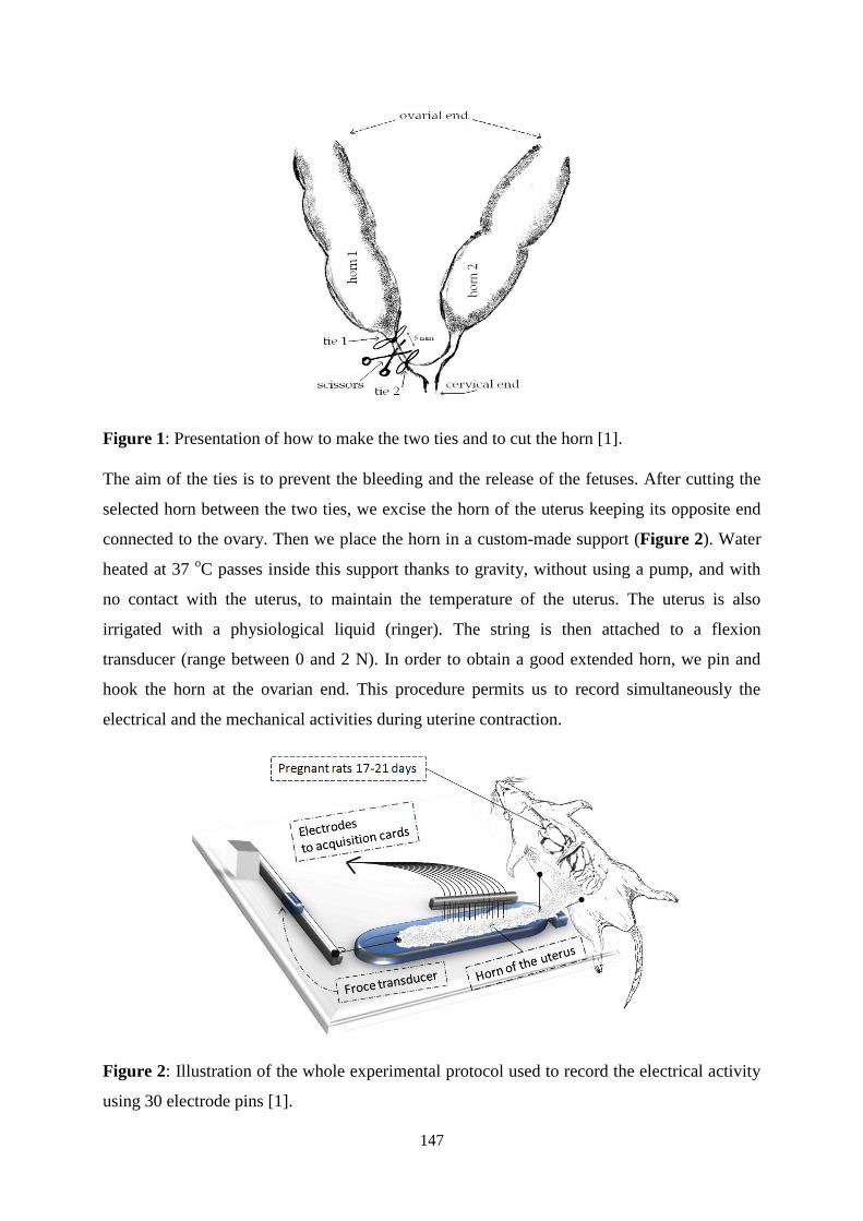
147

Figure 1: Presentation of how to make the two ties and to cut the horn [1].

The aim of the ties is to prevent the bleeding and the release of the fetuses. After cutting the

selected horn between the two ties, we excise the horn of the uterus keeping its opposite end

connected to the ovary. Then we place the horn in a custom-made support (Figure 2). Water

heated at 37 oC passes inside this support thanks to gravity, without using a pump, and with

no contact with the uterus, to maintain the temperature of the uterus. The uterus is also

irrigated with a physiological liquid (ringer). The string is then attached to a flexion

transducer (range between 0 and 2 N). In order to obtain a good extended horn, we pin and

hook the horn at the ovarian end. This procedure permits us to record simultaneously the

electrical and the mechanical activities during uterine contraction.

Figure 2: Illustration of the whole experimental protocol used to record the electrical activity

using 30 electrode pins [1].

148

In order to be able to record the electrical and mechanical activity simultaneously, great care

was taken in the positioning of the horn of the uterus and of the electrode. We thus developed

an adapted suction electrode device. A cuboid of length = 12 cm, width = 4 cm, and height =

5 cm was made by 6 faces of Plexiglas glued carefully to make it waterproof. 32 holes were

perforated in the bottom and the top faces of the cuboid, 30 holes for the uterine EMG

electrodes and 2 for the reference electrodes (Figure 3).

Two other holes were perforated also on one side face of the cuboid, one connected to a

syringe for suction and a second that could be connected to an intra-cuboid pressure sensor.

As we did not use the pressure sensor for the first experiments we sealed it as shown in

Figure 4 to avoid leakage.

Figure 3: Bottom face of the electrode matrix, we can see the 32 holes.

Figure 4: Side of the electrode matrix, we can see the connectors for the syringe and the

pressure sensor, which is sealed, being unused for these first experiments.

Then we inserted 32 glass capillaries into the holes of the bottom face by keeping space

between the introduced capillaries and the upper face, and we glued them around the holes to

keep the cuboid waterproof. After that we introduce the electrodes wires (red wires in Figure

5-left) from the holes of the upper face into the capillaries until they reach the end of the

capillaries. We them glued around the holes to prevent leakage. The outside parts of the

capillaries were wrapped at the end by rubber (Figure 5-right), to protect them.

Toward

syringe

Sealed pressure

sensor output

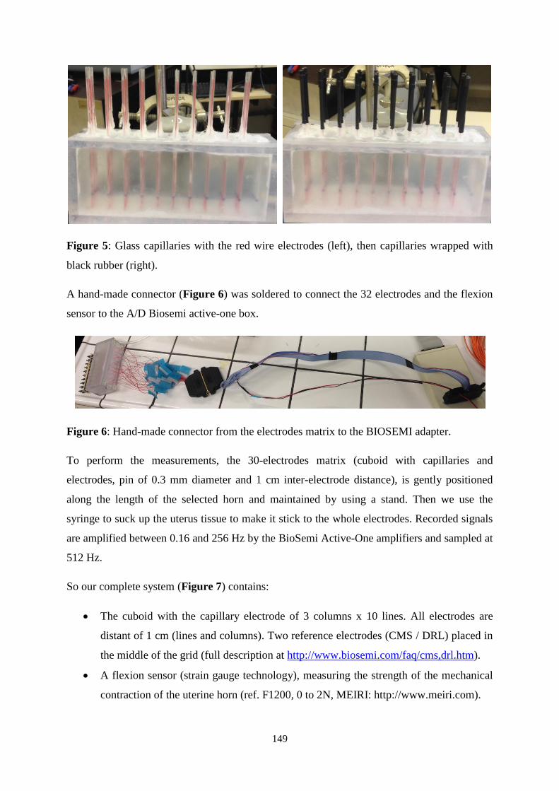
149

Figure 5: Glass capillaries with the red wire electrodes (left), then capillaries wrapped with

black rubber (right).

A hand-made connector (Figure 6) was soldered to connect the 32 electrodes and the flexion

sensor to the A/D Biosemi active-one box.

Figure 6: Hand-made connector from the electrodes matrix to the BIOSEMI adapter.

To perform the measurements, the 30-electrodes matrix (cuboid with capillaries and

electrodes, pin of 0.3 mm diameter and 1 cm inter-electrode distance), is gently positioned

along the length of the selected horn and maintained by using a stand. Then we use the

syringe to suck up the uterus tissue to make it stick to the whole electrodes. Recorded signals

are amplified between 0.16 and 256 Hz by the BioSemi Active-One amplifiers and sampled at

512 Hz.

So our complete system (Figure 7) contains:

The cuboid with the capillary electrode of 3 columns x 10 lines. All electrodes are

distant of 1 cm (lines and columns). Two reference electrodes (CMS / DRL) placed in

the middle of the grid (full description at http://www.biosemi.com/faq/cms,drl.htm).

A flexion sensor (strain gauge technology), measuring the strength of the mechanical

contraction of the uterine horn (ref. F1200, 0 to 2N, MEIRI: http://www.meiri.com).

http://www.biosemi/

150

The amplification is provided by a BIOSEMI A/D box, with sampling accuracy of 24

bits and sampling frequency of 512 Hz. These signals are transmitted by optical fiber

to the computer.

The Actiview software (BIOSEMI) allows the collection and the storage of signals.

Figure 7: Description of the entire system.

Discussion

The new ex-vivo experimental protocol and the improved instrumentation should allow the

recording of the electrical activity of the uterus while keeping it connected to the rat. This

permits to maintain vascularization of the uterus tissue and then to prevent the use of a pump

for oxygenation of the tissue. Our modification to the measurement matrix overcomes the

problem of the curvature of the uterus horn by using a suction system. It also overcomes the

problem of interference between the electrodes due to the capillaries covered by rubber.

By using this system, we measured 4 rats at 17, 19, 20 and 21 days of gestation. But

unfortunately no rat exhibited spontaneous contraction during these experiments. After

verification of the system functioning and the all connections, we concluded that the problem

might come from the anesthetic product. In fact the rats were anesthetized by intraperitoneal

injection into the left part of the abdomen. We thus suspect that the uterine muscle, which

certainly comes in to contact with the anesthetic during this injection, could be inhibited in its

contractile activity. We tried with the last rat to take the horn that is in the right part of the

Stand Electrode

matrix

Uterus

support

Flexion

sensor

Syringe

Connection

adapter

Optical

fiber

Optical/

USB

adapter

A/D

Amplifier battery

Actiview

software

Oscilloscope

Flexion

sensor

conditioner

151

abdomen, but unfortunately this horn was not as developed as the left horn and was too small

for manipulation.

Many improvements should be done in the anesthesia protocol in the future, since we are

limited in materials and time. For example making a pre-anesthesia under hood by gas then

doing the anesthesia by intravenous in the vein of the tail. Thus the anesthesia will not affect

the uterine muscle. Furthermore, a study [5] has shown that an appropriate cocktail of

anesthetic should be used to prevent the paralysis of smooth muscle.

Another reason should be the maintenance of the progesterone block, which is very strong for

rat uterus during all pregnancy. As vascularization is maintained in our protocol, this

progesterone block is present through the maternal blood. Indeed, progesterone withdrawal

has been widely recognized as needed for the initiation of labor in rat uterus. But we were

unable to induce this progesterone withdrawal in our last attempt, even by giving RU486

(strong progesterone inhibitor) to the rat. This protocol has to be refined in further studies.

References:

[1] A. Chkeir, M-J. Fleury, B. Karlsson, M. Hassan, and C. Marque, “Patterns of electrical activity

synchronization in the pregnant rat uterus,” BioMedicine, vol. 3, no. 3, pp. 140-144, Sep. 2013.

[2] S. Rihana, “Modélisation de l'activité électrique utérine,” Phd. dissertation, Université de

technologie de Compiègne, 2008, Compiègne.

[3] W.J. Lammers, B. Stephen, R. Hamid, and D.W.G. Harron, “The effects of oxytocin on the

pattern of electrical propagation in the isolated pregnant uterus of the rat,” Pflügers Archiv, vol

437, no. 3, pp. 363-370, Jan. 1999.

[4] W.J. Lammers, E. El-Kays, K. Arafat, and T.Y. El-Sharkawy, “Wave mapping: detection of

coexisting multiple wavefronts in high-resolution electrical mapping,” Med. Biol. Eng.

Comput., vol. 33, no. 3, pp. 476-81, May. 1995.

[5] J. Laforet, D. Guiraud, D. Andreu, H. Taillades, and C.A. Coste, “Smooth muscle modeling and

experimental identification: application to bladder isometric contraction,” Journal of neural

engineering, vol. 8, no. 3, pp. 036024, May. 2011.

152

Summary:

The uterine EMG -called Electrohysterogramme (EHG)- temporal, frequency, and time-

frequency characteristics have been used for a long time for the prediction of preterm labor.

However, the investigation of its propagation is rare. All the results of the previous studies did

not show a satisfactory potential for clinical application. The objective of this thesis is the

analysis of the propagation as well as of the nonlinear characteristics of EHG signals during

pregnancy and labor for clinical application. A monovariate analysis was done to investigate

the nonlinearity and the sensibility of methods to different characteristics of the signals. A

bivariate analysis was then done for the investigation of the propagation of EHG by

measuring the coupling between channels, as well as the direction of coupling, which is an

innovative part of our thesis. In this analysis we propose a new approach to improve the

coupling and direction estimation methods. Another innovation of this thesis is the

implementation of a tool for EHG source localization to investigate the dynamic of the uterus

at the source level, not at electrodes level as previously done. Results show that nonlinear

methods are more able to classify pregnancy and labor contractions than linear ones, and that

time reversibility method is the least sensitive to sampling frequency and frequency content of

the signal. Results also indicate an increase in coupling and a concentration of coupling

direction toward the cervix when going from pregnancy to labor. We also proposed to respect

the nonstationarity of EHG signal and to recover the effect of variable fat filtering along

pregnancy, by segmenting and filtering the EHG in its FWL component. This filtering-

windowing approach permits to improve the performances of connectivity methods. Finally,

the intensity of localized sources and their number is higher in labor than in pregnancy

contractions. The identified sources are more active and more propagated in labor whereas in

pregnancy they remain weak and local. An improvement in the electrode matrix of the rat

experimental protocol has also been done by developing a suction electrode. This protocol can

then be used for the validation of our methods and of the electrophysiological model.

Keywords:

Prediction of preterm labor, nonlinearity analysis, coupling and direction analysis, source

localization.

153

Résumé:

L'EMG utérin appelé Electrohystérogramme (EHG) a été exploité depuis longtemps par ses

caractéristiques temporelles, fréquentielles, et temps-fréquence, pour la prédiction de

l'accouchement prématuré, tandis que l'étude de sa propagation est rare. Tous les résultats des

études antérieures n'ont pas montré un potentiel satisfaisant pour une application clinique.

L'objectif de cette thèse est l'analyse de la propagation ainsi que de la non-linéarité des

signaux EHG pendant la grossesse et le travail en vue d'une application clinique. Une analyse

monovariée a été faite pour étudier la non-linéarité et la sensibilité des méthodes aux

différentes caractéristiques des signaux. Une analyse bivariée a ensuite été menée pour l‟étude

de la propagation de l‟EHG, en mesurant le couplage entre les voies ainsi que la direction de

couplage, ce qui est une nouveauté de notre thèse. Dans cette analyse, nous proposons une

approche de filtrage-fenêtrage pour améliorer les méthodes d'estimation du couplage et de sa

direction. Une autre nouveauté de cette thèse est l'implantation d'un outil de localisation de

source d'EHG pour étudier la dynamique de l'utérus au niveau de la source, et non pas au

niveau des électrodes comme fait dans les études précédentes. Les résultats montrent que les

méthodes non linéaires sont plus capables que les méthodes linéaires, de classifier les

contractions de grossesse et de travail. La méthode de réversibilité de temps est la moins

sensible à la fréquence d'échantillonnage et au contenu fréquentiel du signal. Les résultats

indiquent également une augmentation de couplage et une concentration des directions vers le

col de l‟utérus, en allant de la grossesse vers le travail. En respectant la non-stationnarité des

signaux EHG et en se libérant de l'effet de filtrage de la graisse, très variable durant la

grossesse et entre les différentes femmes, notre méthode de filtrage-fenêtrage (segmentation

et filtrage du signal EHG pour ne garder que la composant FWL), améliore les performances

des méthodes de connectivité. L'intensité des sources localisées et leur nombre sont plus

élevés durant le travail que durant la grossesse. Les sources localisées sont actives et

propagées durant le travail alors que durant la grossesse elles restent faibles et localisées. Une

amélioration de la matrice d'électrodes du protocole expérimental de rat a été effectuée par le

développement d'une électrode à succion. Ce protocole pourra ensuite être utilisé pour la

validation de nos méthodes et celle du modèle électrophysiologique.

Mots clés:

Prédiction d'accouchement prématuré, analyse non linéaire, analyse de couplage et de

directionalité, localisation de source.

université de technologie de compiègne & reykjavik … · etude théorique et expérimentale...

Documents