universitat politecnica de catalunya` phd progamme ...cuaterniones para representar la rotacion del...
TRANSCRIPT

UNIVERSITAT POLITECNICA DE CATALUNYA
PhD progamme:
Automatic Control, Robotics and Computer Vision
PhD thesis:
Mapping, Planning and Explorationwith Pose SLAM
Rafael Valencia Carreno
Thesis supervisor: Juan Andrade-Cetto
February 2013


Universitat Politecnica de Catalunya
BarcelonaTech (UPC)
PhD progamme:
Automatic Control, Robotics and Computer Vision
The work presented in this thesis has been carried out at:
Institut de Robotica i Informatica Industrial, CSIC-UPC
Thesis supervisor:
Juan Andrade-Cetto
c© Rafael Valencia Carreno 2013


Abstract
This thesis reports research on mapping, path planning, and autonomous exploration. These are
classical problems in robotics, typically studied independently, and here we link such problems
by framing them within a common SLAM approach, adopting Pose SLAM as the basic state
estimation machinery. The main contribution of this thesis is an approach that allows a mobile
robot to plan a path using the map it builds with Pose SLAM and to select the appropriate
actions to autonomously construct this map.
Pose SLAM is the variant of SLAM where only the robot trajectory is estimated and where
landmarks are only used to produce relative constraints between robot poses. In Pose SLAM,
observations come in the form of relative-motion measurements between robot poses. With re-
gards to extending the original Pose SLAM formulation, this thesis studies the computation of
such measurements when they are obtained with stereo cameras and develops the appropriate
noise propagation models for such case. Furthermore, the initial formulation of Pose SLAM
assumes poses in SE(2) and in this thesis we extend this formulation to SE(3), parameterizing
rotations either with Euler angles and quaternions. We also introduce a loop closure test that
exploits the information from the filter using an independent measure of information content
between poses. In the application domain, we present a technique to process the 3D volumet-
ric maps obtained with this SLAM methodology, but with laser range scanning as the sensor
modality, to derive traversability maps that were useful for the navigation of a heterogeneous
fleet of mobile robots in the context of the EU project URUS.
Aside from these extensions to Pose SLAM, the core contribution of the thesis is an ap-
proach for path planning that exploits the modeled uncertainties in Pose SLAM to search for
the path in the pose graph with the lowest accumulated robot pose uncertainty, i.e., the path
that allows the robot to navigate to a given goal with the least probability of becoming lost. An
added advantage of the proposed path planning approach is that since Pose SLAM is agnostic
with respect to the sensor modalities used, it can be used in different environments and with
i

different robots, and since the original pose graph may come from a previous mapping session,
the paths stored in the map already satisfy constraints not easy modeled in the robot controller,
such as the existence of restricted regions, or the right of way along paths. The proposed path
planning methodology has been extensively tested both in simulation and with a real outdoor
robot.
Our path planning approach is adequate for scenarios where a robot is initially guided dur-
ing map construction, but autonomous during execution. For other scenarios in which more
autonomy is required, the robot should be able to explore the environment without any su-
pervision. The second core contribution of this thesis is an autonomous exploration method
that complements the aforementioned path planning strategy. The method selects the appro-
priate actions to drive the robot so as to maximize coverage and at the same time minimize
localization and map uncertainties. An occupancy grid is maintained for the sole purpose of
guaranteeing coverage. A significant advantage of the method is that since the grid is only
computed to hypothesize entropy reduction of candidate map posteriors, it can be computed at
a very coarse resolution since it is not used to maintain neither the robot localization estimate,
nor the structure of the environment. Our technique evaluates two types of actions: exploratory
actions and place revisiting actions. Action decisions are made based on entropy reduction
estimates. By maintaining a Pose SLAM estimate at run time, the technique allows to replan
trajectories online should significant change in the Pose SLAM estimate be detected. The
proposed exploration strategy was tested in a common publicly available dataset comparing
favorably against frontier based exploration.
ii

Resum
Aquesta tesi reporta contribucions als problemes de construccio de mapes, planificacio de tra-
jectories i exploracio amb un robot mobil. Aquests son problemes classics en robotica, els quals
tıpicament s’han estudiat de manera independent; no obstant aixo, en aquesta tesi els enllacem
usant el mateix metode de l’SLAM en la solucio de cada problema. Per a aixo emprem el Pose
SLAM com la maquinaria basica d’estimacio d’estat. La contribucio principal d’aquesta tesi
consisteix en un metode que permet al robot planificar trajectories amb el mapa que ell mateix
ha construıt amb el Pose SLAM, aixı com seleccionar les accions adequades per a construir
aquest mapa de manera autonoma.
El Pose SLAM es una variant de l’SLAM en la qual unicament s’estima la trajectoria
del robot, on les caracterıstiques de l’entorn s’empren solament per a calcular el moviment
relatiu entre poses del robot. En el Pose SLAM les observacions consisteixen en mesures del
moviment relatiu entre poses del robot. Amb el proposit d’estendre la formulacio original
del Pose SLAM, en aquesta tesi s’estudia el calcul de tals mesures quan aquestes s’obtenen
mitjancant cameres estereo i es desenvolupen els models de propagacio de l’error adequats
per a tals casos. Aixı mateix, la formulacio inicial del Pose SLAM assumeix poses en SE(2)
i en aquesta tesi estenem aquesta formulacio para SE(3), emprant tant angles d’Euler com
quaternions per a representar la rotacio del robot. Addicionalment, introduım una prova de
tancament de llacos que explota la informacio del filtre emprant una mesura independent del
contingut d’informacio entre poses. Dins d’aquest context, proposem a mes un metode per a
processar mapes volumetrics en 3D obtinguts amb aquesta metodologia de l’SLAM, pero usant
dades provinents d’un telemetre laser en tres dimensions, per a obtenir mapes de traversabilitat,
els quals van ser utils per a la navegacio de flotes heterogenies de robots mobils en el projecte
Europeu URUS.
A mes d’aquestes extensions al Pose SLAM, la contribucio principal d’aquesta tesi es un
metode per a la planificacio de trajectories que explota les incerteses calculades amb el Pose
iii

SLAM per a cercar la trajectoria en el graf de poses amb la mınima incertesa acumulada de
la pose del robot, es a dir, la trajectoria que permet al robot navegar fins a arribar a una certa
meta amb la menor probabilitat de perdre’s. Ates que el Pose SLAM es agnostic respecte
a la modalitat del sensor que s’utilitzi, un avantatge afegit del nostre metode de planificacio
de trajectories es que es pot emprar en diferents entorns i robots. Aixı mateix, ates que el
graf de poses original prove d’una sessio de construccions de mapes previa, les trajectories
contingudes en el mapa satisfan restriccions que son difıcils de modelar, com l’existencia de
regions restringides de l’entorn o el sentit dels camins. La metodologia de planificacio de
trajectories es va provar tant en bases de dades disponibles al public com en un robot mobil en
entorns exteriors.
El nostre metode de planificacio de trajectories es adequat per els escenaris en els quals
el robot es condueix inicialment de forma manual per a construir el mapa, pero es requereix
que actuı de forma autonoma per a seguir una trajectoria. En els casos en els quals es re-
quereixi una major autonomia, el robot ha de ser capac d’explorar l’entorn per si mateix per a
construir el mapa. Aixı, la segona contribucio mes important d’aquesta tesi consisteix en una
estrategia d’exploracio que complementa al nostre metode de planificacio de trajectories. La
nostra estrategia selecciona les accions que condueixin al robot a maximitzar la cobertura del
seu entorn i al mateix temps minimitzar les incerteses de la seva localitzacio i el mapa. Es
mante un mapa d’ocupacio de reixetes amb l’unic proposit de garantir cobertura. Un avan-
tatge d’aquesta estrategia es que el mapa de reixetes solament s’empra per a fer hipotesi de la
reduccio d’entropia en mapes candidats i no per al calcul de la localitzacio del robot ni para
l’estimacio de la estructura de l’entorn pel que no es necessari calcular-lo amb una resolucio
fina. La nostra estrategia avalua dos tipus d’accions: accions d’exploracio i accions que fan
que el robot torni a llocs en els quals havia estat previament. Les decisions es prenen amb base
en estimacions de la reduccio d’entropia. A mes, aquesta estrategia inclou la possibilitat de re-
planificar trajectories en el cas en els quals es detectin millores significatives en la localitzacio
del robot durant l’execucio de la trajectoria. Aquesta tecnica es va validar mitjancant simula-
cions en bases de dades disponibles de forma publica, obtenint resultats favorables respecte a
tecniques d’exploracio classiques.
iv

Resumen
Esta tesis reporta contribuciones a los problemas de construccion de mapas, planificacion de
trayectorias y exploracion con un robot movil. Estos son problemas clasicos en robotica, los
cuales tıpicamente se han estudiado de forma independiente; sin embargo, en esta tesis los
enlazamos usando el mismo metodo de SLAM en la solucion de cada problema. Para esto
empleamos Pose SLAM como la maquinaria basica de estimacion de estado. La contribucion
principal de esta tesis consiste en un metodo que permite al robot planificar trayectorias con
el mapa que el mismo ha construido con Pose SLAM, ası como seleccionar las acciones ade-
cuadas para construir dicho mapa de manera autonoma.
Pose SLAM es una variante de SLAM en la cual unicamente se estima la trayectoria del
robot, en donde las caracterısticas del entorno se emplean solamente para calcular el movimiento
relativo entre poses del robot. En Pose SLAM las observaciones consisten en medidas del
movimiento relativo entre poses del robot. Con el proposito de extender la formulacion origi-
nal de Pose SLAM, en esta tesis se estudia el calculo de tales medidas cuando estas se obtienen
mediante camaras estereo y se desarrollan los modelos de propagacion del error adecuados
para tales casos. Asimismo, la formulacion inicial de Pose SLAM asume poses en SE(2) y en
esta tesis extendemos dicha formulacion para SE(3), empleando tanto angulos de Euler como
cuaterniones para representar la rotacion del robot. Adicionalmente, introducimos una prueba
de cierre de lazos que explota la informacion del filtro empleando una medida independiente
del contenido de informacion entre poses. Dentro de este contexto, proponemos ademas un
metodo para procesar mapas volumetricos en 3D obtenidos con esta metodologıa de SLAM,
pero usando datos provenientes de un telemetro laser en tres dimensiones, para obtener mapas
de traversabilidad, los cuales fueron utiles para la navegacion de flotas heterogeneas de robots
moviles en el proyecto Europeo URUS.
Ademas de dichas extensiones a Pose SLAM, la contribucion principal de esta tesis es un
metodo para la planificacion de trayectorias que explota las incertezas calculadas con Pose
v

SLAM para buscar la trayectoria en el grafo de poses con la mınima incerteza acumulada de
la pose del robot, es decir, la trayectoria que permite al robot navegar hasta cierta meta con
la menor probabilidad de perderse. Dado que el Pose SLAM es agnostico con respecto a la
modalidad de sensor que se utilice, una ventaja anadida de nuestro metodo de planificacion
de trayectorias es que se puede emplear en distintos entornos y robots. Asimismo, dado que el
grafo de poses original proviene de una sesion de construccion de mapas previa, las trayectorias
contenidas en el mapa satisfacen restricciones que son difıciles de modelar, como la existencia
de regiones restringidas del entorno o el sentido de los caminos. La metodologıa de planifi-
cacion de trayectorias se probo empleando tanto en bases de datos disponibles al publico como
en un robot movil en entonos exteriores.
Nuestro metodo de planificacion de trayectorias es adecuado para los escenarios en los que
el robot se conduce inicialmente de forma manual para construir el mapa, pero se requiere que
actue de forma autonoma para seguir una trayectoria. En los casos en los que se requiera una
mayor autonomıa, el robot debe ser capaz de explorar el entorno por sı mismo para construir
el mapa. Ası, la segunda contribucion mas importante de esta tesis consiste en una estrategia
de exploracion que complementa nuestro metodo de planificacion de trayectorias. Nuestra es-
trategia selecciona las acciones que conduzcan al robot a maximizar la cobertura de su entorno
y al mismo tiempo minimizar las incertezas de su localizacion y el mapa. Se mantiene un mapa
de ocupacion de rejillas con el unico proposito de garantizar cobertura. Una ventaja de dicha
estrategia es que el mapa de rejillas solamente se emplea para hacer hipotesis de la reduccion
de entropıa en mapas candidatos y no para el calculo de la localizacion del robot ni para la es-
timacion de la estructura del entorno, por lo que no es necesario calcularlo con una resolucion
fina. Nuestra estrategia evalua dos tipos de acciones: acciones de exploracion y acciones que
hacen que el robot regrese a lugares en los que habıa estado previamente. Las decisiones se
toman con base en estimaciones de la reduccion de entropıa. Ademas, dicha estrategia incluye
la posibilidad de replanificar trayectorias en el caso en que se detecten mejoras significativas en
la localizacion del robot durante la ejecucion de la trayectoria. Esta tecnica se valido mediante
simulaciones en bases de datos disponibles de forma publica, obteniendo resultados favorables
con respecto a tecnicas de exploracion clasicas.
vi

To Graciela, Silvia, and M. Rafael.


Acknowledgements
I would like to express my gratitude to all the people who made this thesis possible. First
and foremost I would like to thank my supervisor, Juan Andrade-Cetto, for his guidance and
motivation over all these years. I would like to acknowledge him for all the opportunities he
has given me. To Josep Maria Porta for his advice, insightful discussions, and collaborations.
To Jaime Valls Miro and Gamini Dissanayake for their fruitful collaborations and for host-
ing me in the Faculty of Engineering and Information Technology, at the University of Tech-
nology, Sydney. To Viorela Ila for her help during the first part of this thesis, and to Martı
Morta for his valuable collaboration.
I would also like to thank to Agustin, Anaıs, Ernesto, Leonel, Michael, and Oscar for the
good moments in Barcelona, to my office colleagues Aleix, Alex, Eduard, and Gonzalo for
bearing with me during these years, and to Tere and Andres for their valuable help during my
stay at Sydney.
I am grateful to my parents, Silvia and M. Rafael, for their love and unconditional support,
to Moises and Alejandra for their friendship and those great holidays together, and last but not
least I would like to thank to my wife, Graciela, for her love, smiles, and support beyond words
in helping me achieve this.
Finally, I would like to acknowledge all sources of financial support that in one way or
another contributed for the development of this thesis. These include, a PhD scholarship from
the Mexican Council of Science and Technology (CONACYT), a Research Stay Grant from
the Agencia de Gestio d’Ajuts Universitaris i de Recerca of The Generalitat of Catalonia (2010
BE1 00967), the Consolidated Research Group VIS (SGR2009-2013), a Technology Transfer
Contract with the Asociacion de la Industria Navarra, the National Research Projects PAU and
PAU+ (DPI2008-06022 and DPI2011-2751) funded by the Spanish Ministry of Economy and
Competitiveness, and the European Integrated Project ARCAS (FP7-ICT-287617).
ix


Contents
Abstract i
Resum iii
Resumen v
Acknowledgements viii
List of figures xv
Nomenclature xxi
1 Introduction 1
1.1 Summary of contributions . . . . . . . . . . . . . . . . . . . . . . . . . . . . 6
1.2 Publications derived from this thesis . . . . . . . . . . . . . . . . . . . . . . . 7
2 SLAM Front-end 9
2.1 Feature extraction and stereo reconstruction . . . . . . . . . . . . . . . . . . . 10
2.2 Pose estimation . . . . . . . . . . . . . . . . . . . . . . . . . . . . . . . . . . 11
2.2.1 Horn’s method . . . . . . . . . . . . . . . . . . . . . . . . . . . . . . 12
2.2.2 SVD-based solution . . . . . . . . . . . . . . . . . . . . . . . . . . . 14
2.3 Error propagation . . . . . . . . . . . . . . . . . . . . . . . . . . . . . . . . . 15
2.3.1 Matching point error propagation . . . . . . . . . . . . . . . . . . . . 17
2.3.2 Point cloud error propagation . . . . . . . . . . . . . . . . . . . . . . 17
xi

2.3.3 Error propagation tests . . . . . . . . . . . . . . . . . . . . . . . . . . 18
2.4 Bibliographical notes . . . . . . . . . . . . . . . . . . . . . . . . . . . . . . . 23
3 SLAM Back-end 27
3.1 Pose SLAM preliminaries . . . . . . . . . . . . . . . . . . . . . . . . . . . . . 28
3.1.1 State augmentation . . . . . . . . . . . . . . . . . . . . . . . . . . . . 29
3.1.2 State update . . . . . . . . . . . . . . . . . . . . . . . . . . . . . . . . 30
3.1.3 Data association . . . . . . . . . . . . . . . . . . . . . . . . . . . . . 31
3.1.4 State sparsity . . . . . . . . . . . . . . . . . . . . . . . . . . . . . . . 36
3.2 6 DOF Pose SLAM . . . . . . . . . . . . . . . . . . . . . . . . . . . . . . . . 36
3.2.1 Euler angles parameterization . . . . . . . . . . . . . . . . . . . . . . 36
3.2.2 Quaternion parameterization . . . . . . . . . . . . . . . . . . . . . . . 38
3.3 Traversability map building . . . . . . . . . . . . . . . . . . . . . . . . . . . . 41
3.4 Mapping with Pose SLAM . . . . . . . . . . . . . . . . . . . . . . . . . . . . 42
3.4.1 Visual odometry map . . . . . . . . . . . . . . . . . . . . . . . . . . . 42
3.4.2 3D volumetric map . . . . . . . . . . . . . . . . . . . . . . . . . . . . 43
3.4.3 Traversability map . . . . . . . . . . . . . . . . . . . . . . . . . . . . 47
3.5 Bibliographical notes . . . . . . . . . . . . . . . . . . . . . . . . . . . . . . . 47
4 Path planning in belief space with Pose SLAM 53
4.1 Path planning with Pose SLAM . . . . . . . . . . . . . . . . . . . . . . . . . 57
4.1.1 Increasing graph connectivity . . . . . . . . . . . . . . . . . . . . . . 58
4.1.2 Uncertainty of a path step . . . . . . . . . . . . . . . . . . . . . . . . 59
4.1.3 Minimum uncertainty along a path . . . . . . . . . . . . . . . . . . . . 61
4.2 The Pose SLAM path planning algorithm . . . . . . . . . . . . . . . . . . . . 62
4.3 Experimental results . . . . . . . . . . . . . . . . . . . . . . . . . . . . . . . 64
4.3.1 Synthetic dataset . . . . . . . . . . . . . . . . . . . . . . . . . . . . . 64
4.3.2 Indoor dataset . . . . . . . . . . . . . . . . . . . . . . . . . . . . . . . 66
xii

4.3.3 Large scale dataset . . . . . . . . . . . . . . . . . . . . . . . . . . . . 71
4.3.4 Dense 3D mapping dataset . . . . . . . . . . . . . . . . . . . . . . . . 74
4.3.5 Real robot navigation . . . . . . . . . . . . . . . . . . . . . . . . . . . 79
4.4 Bibliographical notes . . . . . . . . . . . . . . . . . . . . . . . . . . . . . . . 82
5 Active Pose SLAM 87
5.1 Action set . . . . . . . . . . . . . . . . . . . . . . . . . . . . . . . . . . . . . 88
5.1.1 Exploratory actions . . . . . . . . . . . . . . . . . . . . . . . . . . . . 90
5.1.2 Place re-visiting actions . . . . . . . . . . . . . . . . . . . . . . . . . 91
5.2 Utility of actions . . . . . . . . . . . . . . . . . . . . . . . . . . . . . . . . . 92
5.3 Replanning . . . . . . . . . . . . . . . . . . . . . . . . . . . . . . . . . . . . 94
5.4 Experiments . . . . . . . . . . . . . . . . . . . . . . . . . . . . . . . . . . . . 94
5.4.1 Exploration . . . . . . . . . . . . . . . . . . . . . . . . . . . . . . . . 96
5.4.2 Replanning . . . . . . . . . . . . . . . . . . . . . . . . . . . . . . . . 96
5.4.3 Comparison with frontier-based exploration . . . . . . . . . . . . . . . 97
5.5 Bibliographical notes . . . . . . . . . . . . . . . . . . . . . . . . . . . . . . . 99
5.5.1 Coverage mechanisms . . . . . . . . . . . . . . . . . . . . . . . . . . 99
5.5.2 Objective functions . . . . . . . . . . . . . . . . . . . . . . . . . . . . 101
5.5.3 Action Selection . . . . . . . . . . . . . . . . . . . . . . . . . . . . . 102
6 Conclusions 105
xiii


List of Figures
1.1 System architecture and thesis outline. . . . . . . . . . . . . . . . . . . . . . . 5
2.1 SIFT correspondences in two consecutive stereo image pairs after outlier re-
moval using RANSAC. . . . . . . . . . . . . . . . . . . . . . . . . . . . . . . 12
2.2 Simulation of error propagation for the stereo reconstruction of a single image
pair. The covariance obtained by Monte Carlo simulation is represented by the
black ellipse, while the covariance computed with the first-order error propa-
gation is plotted with the dashed green ellipse. All hyperellipsoids represent
iso-uncertainty curves plotted at a scale of 2 standard deviations. The red point
shows the mean of reconstructed 3D point. . . . . . . . . . . . . . . . . . . . 19
2.3 Simulation of the error propagation of the pose estimation from the two point
clouds. The covariance obtained by Monte Carlo simulation is respresent by
the black ellipse, while the covariance computed with the implicit function
theorem is plotted with the dashed green ellipse. All hyperellipsoids represent
iso-uncertainty curves plotted at a scale of 2 standard deviations. The red point
shows the mean of the estimated pose. . . . . . . . . . . . . . . . . . . . . . . 21
2.4 Some of the SIFT correspondences in two consecutive stereo image pairs and
their covariance. The ellipses represent iso-uncertainty curves plotted at a scale
of 3 standard deviations. . . . . . . . . . . . . . . . . . . . . . . . . . . . . . 23
xv

2.5 Error propagation of the relative pose estimation between two robot poses us-
ing stereo images. The covariance obtained by Monte Carlo simulation is re-
spresent by the black ellipse, while the covariance computed with the implicit
function theorem is plotted with the dashed green ellipse. All hyperellipsoids
represent iso-uncertainty curves plotted at a scale of 2 standard deviations. The
red point shows the mean of the estimated pose. . . . . . . . . . . . . . . . . 24
3.1 A mobile robot has performed a loop trajectory. a) Prior to adding the infor-
mation relevant to the loop, a match hypothesis must be confirmed. If asserted,
we could change the overall uncertainty in the trajectory from the red hyperel-
lipsoids to the ones in blue. b) If the test is made using conventional statistical
tools, such as the Mahalanobis test, all the possible data association links in-
dicated in blue should be verified. With a test based in information content
just the links indicated in red should be verified. c) A loop closure event adds
only a few non-zero off-diagonal elements to the sparse information matrix
(see zoomed region). . . . . . . . . . . . . . . . . . . . . . . . . . . . . . . . 33
3.2 Pose SLAM map built with encoder odometry and stereo vision data. . . . . . . 44
3.3 3D laser range finder mounted on our robotic platform. . . . . . . . . . . . . . 45
3.4 6D range-based SLAM results. . . . . . . . . . . . . . . . . . . . . . . . . . . 46
3.5 Final 3D map of the experimental site computed with our approach. . . . . . . 48
3.6 Traversability map from 2D layers of the aligned 3D point clouds. . . . . . . . 49
4.1 Path planning using the map generated by the Pose SLAM algorithm. (a) The
Pose SLAM map. The red dots and lines represent the estimated trajectory,
and the green lines indicate loop closure constraints established by registering
sensor readings at different poses. (b) A plan in configuration space would pro-
duce the shortest path to the goal. At one point during path execution, sensor
registration fails and the robot gets lost. This happens when the robot is out-
side the sensor registration area for a given waypoint in the tracked trajectory.
The areas around each pose where registration is possible are represented by
rectangles. (c) A plan in belief space produces the minimum uncertainty path
to the goal. Plans with low uncertainty have higher probability of success. . . . 55
xvi

4.2 Zoomed view of a region along the shortest path in Fig. 4.1 where the robot gets
lost. Bad localization on this path leads the robot to deviate from the next way-
point, producing failed sensor registration. The rectangles indicate the areas
where sensor registration is reliable (shown in black for the poses in the map
and in red for the poses in the executed trajectory), the green lines represent
sensor registration links between poses in the executed trajectory and those in
the map, and the blue lines and ellipses represent the localization estimates for
the executed trajectory. . . . . . . . . . . . . . . . . . . . . . . . . . . . . . . 56
4.3 Accumulated cost along the shortest (red) and minimum uncertainty (blue)
paths in the simulated experiment. . . . . . . . . . . . . . . . . . . . . . . . . 65
4.4 Monte Carlo realization of the simulated experiment. The minimum uncer-
tainty path guarantees path completion during localization as indicated by the
blue trajectories. The red dots indicate on the other hand, the points where the
robot gets lost due to a missed sensor registration, while executing the shortest
path. . . . . . . . . . . . . . . . . . . . . . . . . . . . . . . . . . . . . . . . . 66
4.5 Path planning over the Intel dataset. (a) Pose SLAM map built with encoder
odometry and laser scans. The blue arrow indicates the final pose of the robot
and the black ellipse the associated covariance at a 95% confidence level. (b)
Planning in configuration space we obtain the shortest path to the goal on the
underlying Pose SLAM graph. (c) Planning in belief space we obtain the min-
imum uncertainty path to the goal. . . . . . . . . . . . . . . . . . . . . . . . . 67
4.6 Accumulated cost versus the path length for the shortest path (red) and mini-
mum uncertainty path (blue) in the Intel experiment. . . . . . . . . . . . . . . 68
4.7 Plots of execution time and memory footprint when planning with different
subsets of the Intel map and employing two different strategies to recover
marginals. (a) Execution time needed to recover only the marginals (contin-
uous line) and for the whole planning algorithm (dashed line). (b) Memory
footprint for marginal recovery. . . . . . . . . . . . . . . . . . . . . . . . . . . 69
4.8 Path planning over the Manhattan dataset. (a) Planning in configuration space
we obtain the shortest path to the goal on the underlying Pose SLAM graph.
(b) Planning in belief space we obtain the minimum uncertainty path to the goal. 70
xvii

4.9 Accumulated cost along the shortest (red) and minimum uncertainty (blue) path
in the Manhattan experiment. . . . . . . . . . . . . . . . . . . . . . . . . . . . 71
4.10 Path planning over a section of the Manhattan dataset. (a) Planning in config-
uration space we obtain the shortest path to the goal on the underlying Pose
SLAM graph. (b) Planning in belief space we obtain the minimum uncertainty
path to the goal. (c) A minimum uncertainty path to the goal computed when
the marginal covariances are recovered with Markov blankets. . . . . . . . . . 72
4.11 Accumulated cost along the shortest (red) and along the minimum uncertainty
path computed with exact marginal covariances (blue) and with Markov blan-
kets (black). . . . . . . . . . . . . . . . . . . . . . . . . . . . . . . . . . . . . 73
4.12 A close in on the computed 3D range map and the robot trajectory. . . . . . . . 74
4.13 Segway RMP 400 robotic platform at the FME plaza. . . . . . . . . . . . . . . 75
4.14 3D Pose SLAM map of the FME plaza, with the robot trajectory shown in red. . 76
4.15 (a) Planning in configuration space we obtain the shortest path to the goal and
related covariances. (b) Planning in belief space we obtain the minimum un-
certainty path to the goal. . . . . . . . . . . . . . . . . . . . . . . . . . . . . . 77
4.16 Accumulated cost along the shortest path (red) and the minimum uncertainty
path (blue). . . . . . . . . . . . . . . . . . . . . . . . . . . . . . . . . . . . . 78
4.17 Pose SLAM map built with encoder odometry and laser data in an outdoor
scenario with a Segway RMP 400 robotic platform. . . . . . . . . . . . . . . . 80
4.18 Path planning over the map built with our mobile robot using encoder odometry
and laser data. . . . . . . . . . . . . . . . . . . . . . . . . . . . . . . . . . . . 81
4.19 Accumulated cost along the shortest (red) and minimum uncertainty (blue) path
in the real robot experiment. . . . . . . . . . . . . . . . . . . . . . . . . . . . 82
4.20 Real path execution of the shortest and safest paths to the goal with our mobile
robot. The green line shows the planned paths computed with our method.
The red lines represent the obtained trajectories when executing each path five
times. The execution is interrupted when the deviation with respect to the
intended plan is above a safety threshold. . . . . . . . . . . . . . . . . . . . . 83
xviii

5.1 The Pose SLAM posterior is used to render an occupancy map, which is used
to generate candidate paths. (a) Pose SLAM map. (b) Gridmap and frontiers
(red cells). (c) Candidate paths and their utilities. . . . . . . . . . . . . . . . . 89
5.2 Three points in time during the exploration process. At time step 26 (frames a
and b), the robot has the following reduction in entropy: Action 1 = 1.1121 nats,
Action 2 = 1.2378 nats, and Action 3 = 0.7111 nats. At time step 39 (frames
c and d) Action 1 = 1.7534 nats, Action 2 = 1.4252 nats, and Action 3 =
1.1171 nats. Finally, at time step 52 (frames e and f), Action 1 = 1.8482 nats,
Action 2 = 2.0334 nats, and Action 3 = 1.7042 nats. The actions chosen are 2,
1, and 2, respectively. . . . . . . . . . . . . . . . . . . . . . . . . . . . . . . . 95
5.3 Entropy evolution. . . . . . . . . . . . . . . . . . . . . . . . . . . . . . . . . . 97
5.4 Exploration with and without replanning. (a) Pose SLAMmap and (b) gridmap
made without replanning, with a final map entropy of 147.89 nats. (c) Pose
SLAM map and (d) gridmap made with replanning, with a final map entropy
of 146.23 nats. . . . . . . . . . . . . . . . . . . . . . . . . . . . . . . . . . . . 98
5.5 Path entropy evolution with replanning (continuous line) and without replan-
ning (dashed line). . . . . . . . . . . . . . . . . . . . . . . . . . . . . . . . . 99
5.6 Frontier-based exploration. The final map entropy is only reduced to 152.62 nats.
Contrary to the proposed approach, this technique does not evaluate the need
for loop closure and as a consequence, severe localization errors are evident at
the end of the trajectory. . . . . . . . . . . . . . . . . . . . . . . . . . . . . . 100
xix


Nomenclature
Notation
c occupancy of a gridmap cell.
dM Mahalanobis distance.
dB Battacharyya distance.
dr squared distance between two robot positions.
I mutual information gain.
pt probability of a pose being closer than vt to another along dimension t.
s probability threshold for the closeness of two robot poses.
t index of the dimensions of the displacement distribution d.
uo, vo camera image centers.
Uk uncertainty of a path step, from time k − 1 to k.
∆U+k positive increment of individual step cost.
v threshold for the squared distance between two robot positions.
vt distance from one robot pose to another along dimension t.
V index of the predecessor of a node in a graph of poses.
w cell size.
W (r1:T ) mechanical work along path r1:T in the uncertainty surface.
xxi

αu, αv focal lengths.
γ information gain threshold.
ǫ average normalized state estimation error squared.
ǫi normalized state estimation error squared of the ith-Monte Carlo run.
θ pitch angle.
φ yaw angle.
ψ roll angle.
a a three-dimensional vector with the last element equal to zero.
c centroid of a point cloud.
d relative displacement in belief space.
g goal pose.
p three-dimensional scene point.
p three-dimensional scene point shifted to its point cloud’s centroid.
q quaternion with imaginary part qv and scalar part qw.
st start pose.
uk motion command at time k.
v measurement error.
w motion error.
xi robot configuration at time i.
xk Pose SLAM state vector at time k.
x′ simulated Pose SLAM state vector.
zk measurement vector at time k.
xxii

η information vector.
ν directional vector.
0m×n a matrix of zeros of sizem× n.
A+ pseudoinverse of matrix A.
F robot motion Jacobian.
H measurement Jacobian.
Hd Jacobian of the the squared distance between two robot positions.
In identity matrix of n× n.
Om occupancy gridmap.
R, t rotation matrix and translation vector.
S innovation covariance matrix.
UΣV⊤ singular value decomposition.
∇f the Jacobian of function f .
Λ information matrix.
Σd covariance of a relative pose measurement.
Σii marginal covariance corresponding to the ith-pose.
Σp covariance of a three-dimensional scene point.
ΣP a block diagonal matrix containing the covariance of two clouds of points.
Σu motion command error covariance.
Σz measurement error covariance.
C(x,y) a cost function relating the implicit function y = f(x).
erf (·) the error function.
xxiii

f (·) robot motion model.
h (·) measurement model.
H(X) entropy.
H(X|Y ) conditional entropy.
N (µ,Σ) Gaussian distribution with mean µ and covariance Σ.
rot (φ, θ, ψ) rotation matrix as a function of the ZYX-Euler angles.
Φ(x,y) a differentiable function relating the implicit function y = f(x).
χ2n Chi-squared distribution with n degrees of freedom.
A action space.
M graph of robot poses.
p a robot path.
Q set of nodes from a graph of robot poses.
r1:T path from robot pose r1 to rT .
p(i)j the ith-element of the jth-point cloud.
P set of two point clouds.
Uk set of motion commands up to time k.
U ′ candidate set of actions.
V set of linear velocity controls.
Zk set of measurements up to time k.
Z ′ set of hypothesized observations.
Ω set of angular velocity controls.
⊗ quaternion multiplication operator.
xxiv

⊕ Euclidean vector composition operator.
⊖ Euclidean vector inversion operator.
Acronyms
2D Two-dimensional.
3D Three-dimensional.
BRM Belief roadmap.
DOF Degrees of freedom.
EIF Extended Information Filter.
EKF Extended Kalman Filter.
ICP Iterative closest point.
NEES Normalized state estimation error squared.
PRM Probabilistic roadmap.
RANSAC Random sample consensus.
ROS Robot operating system.
SIFT Scale-invariant feature transform.
SLAM Simultaneous localization and mapping.
VO Visual Odometry.
xxv


Chapter 1
Introduction
Simultaneous localization and mapping (SLAM) is the process where a mobile robot builds a
map of an unknown environment while at the same time being localized relative to this map.
Performing SLAM is a basic task for a truly autonomous robot. Consequently, it has been
one of the main research topics in robotics for the last two decades. Whereas in the seminal
approaches to SLAM [151] only few tens of landmarks could be managed, state of the art
approaches can now efficiently manage thousands of landmarks [53, 83, 166] and build maps
over several kilometers [146].
Despite these important achievements in SLAM research, very little has been investigated
concerning approaches that allow the robot to actually employ the maps it builds for navigation.
Aside from applications such as the reconstruction of archaeological sites [44] or the inspection
of dangerous areas [167], the final objective for an autonomous robot is not to build a map of the
environment, but to use this map for navigation. Another issue that has not received extensive
attention is the problem of autonomous exploration for SLAM. Most SLAM techniques are
passive in the sense that the robot only estimates the model of the environment, but without
taking any decisions on its trajectory.
The main goal of this thesis is to contribute with an approach that allows a mobile robot
to plan a path using the map it builds with SLAM and to select the appropriate actions to
autonomously construct this map. In addition, it studies related issues such as visual odometry
and 3Dmapping. Thus, this thesis reports research on mapping, path planning, and autonomous
exploration. These are classical problems in robotics, typically studied independently, and here
we link such problems by framing them within a common SLAM approach.
1

In this thesis we adopt the Pose SLAM approach [69] as the basic state estimation machin-
ery. Pose SLAM is the variant of SLAMwhere only the robot trajectory is estimated and where
landmarks are only used to produce relative constraints between robot poses. Thus, the map
in Pose SLAM only contains the trajectory of the robot. The poses stored in the map are, by
construction, feasible and obstacle-free since they were already traversed by the robot when
the map was originally built. Additionally, Pose SLAM only keeps non-redundant poses and
highly informative links. Thus, the state does not grow independently of the size of the environ-
ment. It also translates into a significant reduction of the computational cost and a delay of the
filter inconsistency, maintaining the quality of the estimation for longer mapping sequences.
In Pose SLAM, observations come in the form of relative-motion measurements between
any two robot poses. This thesis studies the computation of such measurements when they are
obtained with stereo cameras and presents an implementation of a visual odometry method that
includes a noise propagation technique.
The initial formulation of Pose SLAM [69] assumes poses in SE(2) and in this thesis we
extend this formulation to poses in SE(3), parameterizing rotations either with Euler angles and
quaternions. We also introduce a loop closure test tailored to Pose SLAM that exploits the in-
formation from the filter using an independent measure of information content between poses,
which for consistent estimates is less affected by perceptual aliasing. Furthermore, we present
a technique to process the 3D volumetric maps obtained with this SLAM implementation in
SE(3) to derive traversability maps useful for the navigation of a heterogeneous fleet of mobile
robots.
Besides the aforementioned advantages of Pose SLAM, a notable property of this approach
for the purposes of this thesis is that, unlike standard feature-based SLAM, its map can be
directly used for path planning. The reason that feature-based SLAM cannot be directly used
to plan trajectories is that these methods produce a sparse graph of landmark estimates and
their probabilistic relations, which is of little value to find collision free paths for navigation.
These graphs can be enriched with obstacle related information [59, 121, 137], but it increases
the complexity. On the contrary, as the outcome of Pose SLAM is a graph of obstacle-free
paths in the area where the robot has been operated, this map can be directly employed for path
planning.
In this thesis we propose an approach for path planning under uncertainty that exploits
the modeled uncertainties in robot poses by Pose SLAM to search for the path in the pose
2

graph with the lowest accumulated robot pose uncertainty, i.e., the path that allow the robot to
navigate to the goal without becoming lost.
The approach from the motion planning literature that best matches our path planning ap-
proach is the Belief Roadmap (BRM) [62, 134]. In such an approach, the edges defining the
roadmap include information about the uncertainty change when traversing such an edge. How-
ever, the main drawback of the BRM is that it still assumes a known model of the environment,
which is in general not available in real applications. In contrast, we argue in this thesis that
Pose SLAM graphs can be directly used as belief roadmaps.
An added advantage of our path planning approach is that Pose SLAM is agnostic with
respect to the sensor modalities used, which facilitates its application in different environments
and robots, and the paths stored in the map satisfy constraints not easy to model in the robot
controller, such as the existence of restricted regions, or the right of way along paths.
Our path planning approach is adequate for scenarios where a robot is initially guided dur-
ing map construction, but autonomous during execution. For other scenarios in which more
autonomy is required, the robot should be able to explore the environment without any super-
vision. In this thesis we also introduce an autonomous exploration approach for the case of
Pose SLAM, which complements the path planning method.
A straightforward solution to the problem of exploration for SLAM is to combine a classi-
cal exploration method with SLAM. However, classical exploration methods focus on reducing
the amount of unseen area disregarding the cumulative effect of localization drift, leading the
robot to accumulate more and more uncertainty. Thus, a solution to this problem should revisit
known areas from time to time, trading off coverage with accuracy.
In this thesis we propose an autonomous exploration strategy for the case of Pose SLAM
that automates the belief roadmap construction from scratch by selecting the appropriate ac-
tions to drive the robot so as to maximize coverage and at the same time minimize localization
and map uncertainties. In our approach, we guarantee coverage with an occupancy grid of the
environment. A significant advantage of the approach is that this grid is only computed to hy-
pothesize entropy reduction of candidate map posteriors, and that it can be computed at a very
coarse resolution since it is not used to maintain neither the robot localization estimate, nor the
structure of the environment. In a similar way to [157], our technique evaluates two types of
actions: exploratory actions and place revisiting actions. Action decisions are made based on
entropy reduction estimates. By maintaining a Pose SLAM estimate at run time, the technique
3

allows to replan trajectories online should significant change in the Pose SLAM estimate be
detected, something that would make the computed entropy reduction estimates obsolete.
This thesis is structured in three parts. The first is devoted to the SLAM approach we em-
ploy along the thesis. The second part introduces our algorithm for planning under uncertainty.
Finally, in the last part we present an exploration approach to automate the map building pro-
cess with Pose SLAM. Fig. 1.1 shows a block diagram representing the system architecture
proposed in this thesis that also outlines the structure of this document.
In this thesis we follow the abstraction of SLAM usually employed by Pose graph SLAM
methods [57, 128], which divide SLAM in a front-end and a back-end part. Thus, the first
part of the thesis is split in two chapters. We begin our discussion by presenting our SLAM
front-end in Chapter 2, which is in charge of processing the sensor information to compute the
relative-motion measurements. In the context of this thesis observations come in the form of
relative-motion constraints between two robot poses. These are typically computed using the
Iterative Closest Point (ICP) method [15] when working with laser scans. When working with
stereo images, visual odometry techniques are usually employed to recover the relative-pose
measurements. The latter method is adopted in our contribution presented at IROS 2007 [68]
and in Chapter 2 we describe it in more detail and introduce a technique to model the mea-
surements noise, which propagates the noise in image features to relative-pose measurements.
Next, in Chapter 3, we present the back-end part of Pose SLAM, that is, the related to the
state estimation task, which is sensor agnostic. We begin with an exposition of the basics of
Pose SLAM based on the work by Eustice et al. [43] and Ila et al. [69]. In this exposition we
also include one of our initial contributions, consisting of a loop closure test for Pose SLAM,
presented at IROS 2007 [68]. Next, we discuss the extension of Pose SLAM to deal with poses
in SE(3) and show results on its application to build 3D volumetric maps and traversability
maps. Such results were presented at IROS 2009 [172] and were developed as part of the
European Union-funded project “Ubiquitous networking robotics in urban settings” (URUS)
[141]. Furthermore, the maps we built were also employed for the calibration of a camera
network tailored for this project, whose results were presented at the Workshop on Network
Robot Systems at IROS 2009 [2].
The second part of this thesis deal with the problem of path planning with SLAM. Chap-
ter 4 details our path planning method. It describes how to plan a path using the roadmap
built with Pose SLAM, presents the new planning approach, and shows results with datasets
4

Robot
Path Planning
[Chapter 4]
Exploration
[Chapter 5]
Motion commands
Back-End
[Chapter 3]
Front-End
[Chapter 2]Pose
constraints
Pose SLAM estimate
SLAM
Raw sensor measurements
Figure 1.1: System architecture and thesis outline.
and real world experiments with a four-wheel mobile robot. An initial version of this approach
was documented in a technical report [170] and, eventually, an improved version was presented
at ICRA 2011 [169]. A journal version of this work that includes more improvements as well
as real world experiments is conditionally accepted for publication at IEEE Transactions on
Robotics [171]. Furthermore, results on path planning with 3D volumetric maps appeared at
5

1.1 Summary of contributions
the Spanish workshop ROBOT’11 [160].
Lastly, our autonomous exploration strategy for Pose SLAM is presented in Chapter 5.
This part of the thesis was carried out during my stay at the Centre for Autonomous Systems,
in the Faculty of Engineering and Information Technology, at the University of Technology,
Sydney. The results of this approach were presented at IROS 2012 [173] and we are currently
working on a journal submission on this work.
1.1 Summary of contributions
The contributions presented in this thesis constitute a step towards an integrated framework for
mapping, planning and exploration for autonomous mobile robots. These contributions can be
grouped by each of these three problems as follows:
• We introduce a visual odometry technique (Chapter 2), a loop closure strategy for Pose
SLAM, an extension of Pose SLAM to work with poses in 6 DOF, and a method to com-
pute traversability maps (Chapter 3).
We present an implementation of a visual odometry method that includes a noise prop-
agation technique. We also introduce a loop closure test tailored to Pose SLAM that
exploits the information from the filter using an independent measure of information con-
tent between poses, which for consistent estimates is less affected by perceptual aliasing.
We extend Pose SLAM [69] to deal with poses in SE(3), parameterizing rotations either
with Euler angles and quaternions. Furthermore, we introduce a technique to process the
3D volumetric maps obtained with our 3D SLAM implementation to derive traversability
maps useful for the navigation of a heterogeneous fleet of mobile robots.
• We present a path planning method in belief space (Chapter 4) that computes the most
reliable path to the goal in a pose graph computed with Pose SLAM.
From the point of view of SLAM, this method constitutes a step forward to actually use
the output of the mapping process for path planning. From the point of view of motion
planning, the approach contributes with a method to generate belief roadmaps without
resorting to stochastic sampling on a pre-defined environment model. Another feature is
6

1.2 Publications derived from this thesis
that this approach is agnostic to the sensor modality. We validated this contribution with
diverse data sets as well as with real robot implementations.
• Lastly, we contribute with an autonomous exploration strategy (Chapter 5) to automate
the belief roadmap building for Pose SLAM.
The method we presented evaluates the utility of exploratory and place revisiting se-
quences and chooses the one that minimizes overall map and path entropies. An advan-
tage of the proposed strategy with respect to competing approaches is that to evaluate
information gain over the map, only a very coarse prior map estimate needs to be com-
puted. Its coarseness is independent and does not jeopardize the Pose SLAM estimate.
Our approach also allows for a more principled way to determine loop closure actions
by exploiting the data association mechanisms of Pose SLAM. Moreover, a replanning
scheme is devised to detect significant localization improvement during path execution.
1.2 Publications derived from this thesis
The publications derived from the aforementioned contributions are:
• R. Valencia, M. Morta, J. Andrade-Cetto, and J. M. Porta. Planning Reliable Paths with
Pose SLAM. Conditionally accepted for publication in IEEE Transactions on Robotics.
• R. Valencia, J. Valls Miro, G. Dissanayake, and J. Andrade-Cetto. Active Pose SLAM.
In Proceedings of the IEEE/RSJ International Conference on Intelligent Robots and Sys-
tems, 2012, pp. 1885-1891.
• R. Valencia, J. Andrade-Cetto, and J.M. Porta. Path planning in belief space with Pose
SLAM. In Proceedings of the IEEE International Conference on Robotics and Automa-
tion, pages 78-83, Shanghai, May 2011.
• E.H. Teniente, R. Valencia and J. Andrade-Cetto. Dense outdoor 3D mapping and navi-
gation with Pose SLAM. In Proceedings of III Workshop de Robotica: Robotica Exper-
imental, ROBOT’11, Seville, pp. 567-572.
7

1.2 Publications derived from this thesis
• R. Valencia, E.H. Teniente, E. Trulls, and J. Andrade-Cetto. 3D mapping for urban
service robots. In Proceedings of the IEEE/RSJ International Conference on Intelligent
Robots and Systems, pages 3076-3081, Saint Louis, October 2009.
• J. Andrade-Cetto, A.A. Ortega, E.H. Teniente, E. Trulls Fortuny, R. Valencia and A.
Sanfeliu. Combination of distributed camera network and laser-based 3D mapping for
urban service robots. In Proceedings of the IEEE/RSJ IROS Workshop on Network
Robot Systems, 2009, Saint Louis, pp. 69-80.
• V. Ila, J. Andrade-Cetto, R. Valencia, and A. Sanfeliu. Vision-based loop closing for
delayed state robot mapping. In Proceedings of the IEEE/RSJ International Conference
on Intelligent Robots and Systems, pages 3892-3897, San Diego, November 2007.
8

Chapter 2
SLAM Front-end
In this Chapter we discuss our choice of front-end for SLAM, the part in charge of processing
the sensor information to generate the observations that will be fed to the estimation machin-
ery. In the context of this thesis, observations come in the form of relative-motion constraints
between any two robot poses. They are typically obtained with the Iterative Closest Point (ICP)
algorithm [15] when working with laser scans. When using stereo images, the egomotion of
the robot can be estimated with visual odometry [51, 142]. The latter method is adopted in our
contribution presented in [68] and in this Chapter we describe it in more detail and extend it
with a technique to model the uncertainty of the relative-motion constraints.
Assuming we have a pair of stereo images acquired with two calibrated cameras fixed to
the robot’s frame, our approach iterates as follows: SIFT image features [98] are extracted from
the four images and matched between them. The resulting point correspondences are used for
least-squares stereo reconstruction. Next, matching of these 3D features in the two consecutive
frames is used to compute a least-squares best-fit pose transformation, rejecting outliers via
RANSAC [47].
However, the outcome of this approach is also prone to errors. Errors in locating the im-
age features lead to errors in the location of the 3D feature points after stereo reconstruction,
which eventually cause errors in the motion estimate. Modeling such error propagation allows
to compute motion estimates with the appropriate uncertainty bounds. In this Chapter we in-
troduce a technique to compute the covariance of the relative pose measurement by first-order
error propagation [45].
These camera pose constraints are eventually used as relative pose measurements in the
9

2.1 Feature extraction and stereo reconstruction
SLAMwe employ in this thesis. They are used either as odometry measurements, when match-
ing stereo images from consecutive poses in time, or as loop closure constraints, when comput-
ing the relative motion of the last pose with respect to any previous pose. This will be discussed
in Chapter 3.
The rest of this Chapter is structured as follows. Section 2.1 explains the feature extraction
and the stereo reconstruction process. Next, the pose estimation step is shown in Section 2.2.
Then, in Section 2.3 we introduce a technique to model the uncertainty of the relative motion
measurement. Finally, in section 2.4 we provide bibliographical notes.
2.1 Feature extraction and stereo reconstruction
Simple correlation-based features, such as Harris corners [60] or Shi and Tomasi features [145],
are of common use in vision-based SFM and SLAM; from the early uses of Harris himself
to the popular work of Davison [34]. This kind of features can be robustly tracked when
camera displacement is small and are tailored to real-time applications. However, given their
sensitivity to scale, their matching is prone to fail under larger camera motions; less to say for
loop-closing hypotheses testing. Given their scale and local affine invariance properties, we opt
to use SIFTs instead [98, 109], as they constitute a better option for matching visual features
from significantly different vantage points.
In our system, features are extracted and matched with previous image pairs. Then, from
the surviving features, we compute the imaged 3D scene points as follows.
Assumming two stereo-calibrated cameras and a pin-hole camera model [61], with the left
camera as the reference of the stereo system, the following expressions relate a 3D scene point
p to the corresponding points m = [u, v]⊤ in the left, and m′ = [u′, v′]⊤ in the right camera
image planes[
m
s
]
=
αu 0 uo 00 αv vo 00 0 1 0
[
I3 001×3 1
] [
p
1
]
, (2.1)
[
m′
s′
]
=
α′u 0 u′o 00 α′
v v′o 00 0 1 0
[
R t
01×3 1
] [
p
1
]
, (2.2)
where αu and αv are the pixel focal lengths in the x and y directions for the left camera,
and α′u and α′
v for the right camera, (uo, vo) and (u′o, v′o) are the left and right camera image
10

2.2 Pose estimation
centers, respectively. The homogeneous transformation from the right camera frame to the ref-
erence frame of the stereo system is represented by the rotation matrixR and translation vector
t = [tx, ty, tz]⊤. [m⊤, s]⊤ and [m′⊤, s′]⊤ are the left and right image points in homogeneous
coordinates, with scale s and s′, respectively, and I3 is a 3× 3 identity matrix.
Equations 2.1 and 2.2 define the following overdetermined system of equations
(u′ − u′o)r⊤3 − α′ur
⊤1
(v′ − v′o)r⊤3 − α′vr
⊤2
−αu, 0, u− uo0,−αv, v − vo
xyz
=
(u′o − u′)tz + α′utx
(v′o − v′)tz + α′vty
00
Ap = b, (2.3)
whereR is expressed by its row elements
R =
r⊤1r⊤2r⊤3
.
Solving for p in Eq. 2.3 gives the sought 3D coordinates of the imaged points m and m′.
Performing this process for each pair of matching feature in a pair of stereo images results in
two sets of 3D points, or 3D point clouds, i.e.
p(i)1
and
p(i)2
.
2.2 Pose estimation
Next, we present two alternatives to compute the relative motion of the camera from two stereo
images by solving the 3D to 3D pose estimation problem.
The general solution to this problem consists of finding the rotation matrix R and trans-
lation vector t that minimize the squared L2-norm for all points in the two aforementioned
clouds,
R, t
= argminR,t
N∑
i=0
∥
∥
∥p(i)1 −
(
Rp(i)2 + t
)∥
∥
∥
2, (2.4)
with N the number of points in each cloud.
For both methods, we resort to the use of RANSAC [47] to eliminate outliers. It might
be the case that SIFT matches occur on areas of the scene that experienced motion during
the acquisition of the two image stereo pairs. For example, an interest point might appear
at an acute angle of a tree leaf shadow, or on a person walking in front of the robot. The
11

2.2 Pose estimation
Figure 2.1: SIFT correspondences in two consecutive stereo image pairs after outlier removal
using RANSAC.
corresponding matching 3D points will not represent good fits to the camera motion model,
and might introduce large bias to our least squares pose error minimization. The use of such a
robust model fitting technique allows us to preserve the largest number of point matches that at
the same time minimize the square sum of the residuals, as shown in Figure 2.1.
Furthermore, if the covariance of the matching points is available it can be exploited so as
to explicitly model their precision according to their distance from the camera. For instance,
we can weight the point mismatch in Eq. 2.4 with the covariance of the triangulation of the two
points. However, this would complicate further the optimization problem defined by Eq. 2.4.
Instead, we chose to rely on standard techniques such as the following solutions.
2.2.1 Horn’s method
A solution for the rotation matrix R is computed by minimizing the sum of the squared errors
between the rotated directional vectors of feature matches for the two robot poses [65]. Direc-
tional vectors ν are computed as the unit norm direction along the imaged 3D scene point p
12

2.2 Pose estimation
and indicates the orientation of such a point, that is,
ν(i)1 =
p(i)1
‖p(i)1 ‖
(2.5)
and
ν(i)2 =
p(i)2
‖p(i)2 ‖
(2.6)
are the directional vectors for the ith point on the first and the second point cloud, respectively.
The solution to this minimization problem gives an estimate of the orientation of one cloud
of points with respect to the other, and can be expressed in quaternion form as
∂
∂R
(
q⊤Bq)
= 0 , (2.7)
where B is given by
B =N∑
i=1
BiB⊤i , (2.8)
Bi =
0 −c(i)x −c(i)y −c(i)z
c(i)x 0 b
(i)z −b(i)y
c(i)y −b(i)z 0 b
(i)x
c(i)z b
(i)y −b(i)x 0
, (2.9)
and
b(i) = ν(i)2 + ν
(i)1 , c(i) = ν
(i)2 − ν
(i)1 . (2.10)
The quaternion q that minimizes the argument of the derivative operator in the differential
Equation 2.7 is the smallest eigenvector of the matrix B.
If we denote this smallest eigenvector by the 4-tuple (q1, q2, q3, q4)⊤, it follows that the
angle θ associated with the rotational transform is given by
θ = 2cos−1(q4), (2.11)
and the axis of rotation would be given by
a =(q1, q2, q3)
⊤
sin(θ/2). (2.12)
13

2.2 Pose estimation
Then, it can be shown that the elements of the rotation submatrixR are related to the orientation
parameters a and θ by
R =
a2x + (1− a2x)cθ axayc′θ − azsθ axazc
′θ + aysθ
axayc′θ + azsθ a2y + (1− a2y)cθ ayazc
′θ − axsθ
axazc′θ − aysθ ayazc
′θ + axsθ a2z + (1− a2z)cθ
, (2.13)
where sθ = sin θ, cθ = cos θ, and c′θ = 1− cos θ.
Once the rotation matrix R is computed, we can use again the matching set of points to
compute the translation vector t
t =1
N
(
N∑
i=1
p(i)1 −R
N∑
i=1
p(i)2
)
. (2.14)
2.2.2 SVD-based solution
This solution decouples the translational and rotation parts of the pose estimation problem by
noting that, at the least-squares solution to Eq.2.4, both of the two 3D point clouds should have
the same centroid [7].
Thus, the rotation matrix is computed first by reducing the original least-squares problem
to finding the rotation that minimizes
N∑
i=0
∥
∥
∥p(i)1 −
(
Rp(i)2
)∥
∥
∥
2, (2.15)
where
p(i)1 = p
(i)1 − c1 (2.16)
and
p(i)2 = p
(i)2 − c2, (2.17)
express the ith point on the two point clouds translated to their corresponding centroids, with
c1 and c2 the centroids of the first and the second point cloud, respectively.
In order to minimize Eq. 2.15, it is defined the 3× 3 matrix M
M =N∑
i=0
p(i)1 p
(i) ⊤
2 , (2.18)
14

2.3 Error propagation
where its singular value decomposition is given by
M = UΣV⊤. (2.19)
With this, the rotation matrix that minimizes Eq. 2.15 is
R = UV⊤ (2.20)
as long as |UV⊤| = +1. Otherwise, if |UV⊤| = −1, the solution is a reflection.
Finally, having found the rotation R, the translation is computed by
t = c1 − Rc2. (2.21)
2.3 Error propagation
In this section we present a method to model the uncertainty of the relative motion measure-
ments computed with the visual odometry approach just described in this Chapter. This method
propagates the noise from each matching feature, along the visual odometry process, to end up
with a relative pose covariance estimate.
One way to do this is by Monte Carlo simulation, however, this process is time-consuming.
Instead, we opt for a closed-form computation based on first order error propagation. That is,
given a continuously differentiable function y = f(x) and the covarianceΣx of the input x, we
can obtain the covarianceΣy of the output y by linearizing f(x) around the expected value xo
by a first-order Taylor series expansion. Thus, the first-order error propagation to covariance
Σy is given by
Σy = ∇fΣx∇f⊤,
where∇f is the Jacobian of f .
However, sometimes we might not have access to an explicit expression for y = f(x), as it
will be shown to be our case. Fortunately, though, we still can compute an expression for the
Jacobian of f(x) by the implicit function theorem, which we introduce next.
The implicit function theorem can be stated as follows [45]:
Theorem 1. Let S ⊂ Rn × R
m be an open set and let Φ : S → Rm be a differentiable
function. Suppose that (xo,yo) ∈ S that Φ(xo,yo) = 0, and that
∣
∣
∣
∂Φ∂y
∣
∣
∣
(xo,yo)6= 0. Then
15

2.3 Error propagation
there is an open neighborhood X ⊂ Rn of xo, a neighborhood Y ⊂ R
m of yo, and a unique
differentiable function f : X → Y such that
Φ(x, f(x)) = 0
for all x ∈ X .
This theorem tells us that y = f(x) is implicitly defined by Φ(x,y) = 0. Then, if we
differentiateΦ with respect to x we get
∂Φ
∂x+∂Φ
∂f
df
dx= 0.
From this expression we can notice that, by knowing Φ, we can compute the derivative of the
function f with respect to x, even though we do not have an explicit expression for it, that is,
df
dx= −
(
∂Φ
∂y
)−1 ∂Φ
∂x. (2.22)
Next, Φ con be computed as follows. If y = y∗ is a value where a cost function C(x,y)
has a minimum, Φ can be computed by the fact that, at the minimum of this cost function,
∂C(x,y∗)∂y = 0, then we chooseΦ = ∂C
∂y . Thus, by the implicit function theorem, in a neighbor-
hood of y∗ the Jacobian of f is
∇f = −(
∂2C
∂y2
)−1(∂2C
∂y∂x
)⊤
(2.23)
This is the case when the function f is involved in a cost function with no constraints,
otherwise, determining Φ takes additional steps.
For the visual odometry process just described, the error propagation is performed in two
steps. In the first, the covariance of each matching point is propagated through the least-squares
stereo reconstruction process to get the covariance estimate of the corresponding 3D scene
point. In the second step, the covariance of each 3D point of the two point clouds that are
aligned are propagated through the pose estimation process to finally obtain the covariance of
the relative pose measurement.
First order error propagation requires the derivatives of a function that converts matching
points into 3D points in the first step, and 3D point clouds into a pose in the last step. Although
we do not have access to an explicit function for each step, implicit functions are given by each
of the involved minimization processes. Next we show how we compute the ensuing Jacobians.
16

2.3 Error propagation
2.3.1 Matching point error propagation
We want the covariance Σp of the 3D scene point p = [x, y, z]⊤ given the covariance Σm
of the left image matching feature m = [u, v]⊤ and the covariance Σm′ of the right image
matching feature m′ = [u′, v′]⊤. For instance, if we are using SIFT descriptors, the scale at
which each feature was found can be used as an estimate for its covariance.
Next, to findΣp we need to obtain a first-order propagation of the covariance of the uncor-
related matching image feature, which is given by
Σp = ∇g[
Σm 02×2
02×2 Σm′
]
∇g⊤ (2.24)
where ∇g is the Jacobian of the explicit function g that maps a pair of matching image points
u = [u, v, u′, v′]⊤ into its corresponding 3D scene point p, i.e. p = g(u).
As in this step the 3D scene point is found by solving the overdetermined system of equa-
tions given by Eq. 2.3, so as to apply the implicit function theorem, we need to express this
process as an optimization problem. Thus, finding the 3D scene point p can be seen as mini-
mizing the squared L2-norm of the residual of Eq. 2.3, that is,
C(u,p) = ‖Ap− b‖2. (2.25)
Computing the gradient of 2.25 with respect to p and setting it to zero, we find the minimum
at
p∗ = (A⊤A)−1A⊤ b, (2.26)
assumingA to be invertible.
Lastly, having defined Eq. 2.25, by the implicit function theorem, the Jacobian of g is given
by
∇g = −(
∂2C
∂p2
)−1 (∂2C
∂p∂m
)⊤
. (2.27)
2.3.2 Point cloud error propagation
In this step we are looking for the covariance Σd of the relative pose constraint d expressing
the relative motion of the camera, given the covariances of each of the 3D points on the two
point clouds. Here, again, this covariance will be computed by a first-order propagation, and
17

2.3 Error propagation
we will need to compute the Jacobian of a function h that maps the points P =
p(i)1 ,p
(i)2
on the two point clouds into the relative pose d that indicates the relative motion between the
frame of the two clouds, i.e. d = h(P).
If we express the relative pose d using Euler angles to represent its orientation, Eq. 2.4 can
be written as follows
C(P,d) =N∑
i=0
∣
∣
∣
∣
∣
∣
∣
∣
∣
∣
∣
∣
p(i)1 −
rot(φd, θd, ψd)p(i)2 +
xdydzd
∣
∣
∣
∣
∣
∣
∣
∣
∣
∣
∣
∣
2
, (2.28)
where d = [xd, yd, zd, φd, θd, ψd]⊤, rot(φd, θd, ψd) is the rotation matrix defined by the Euler
angles, and N is the point cloud size. The optimal value for d is computed with either one of
the two approaches described in Section 2.2.
Thus, with the implicit function theorem the Jacobian of d = h(P) is given by
∇h = −(
∂2C
∂d2
)−1 (∂2C
∂d∂P
)⊤
. (2.29)
Finally, the covariance Σd of the relative pose constraint d will be given by,
Σd = ∇hΣP∇h⊤, (2.30)
where ΣP is the covariance of the two clouds of points P, that is,
ΣP = diag(
Σ(1)p1 , ...,Σ
(N)p1 ,Σ
(1)p2 , ...,Σ
(N)p2
)
, (2.31)
which is a block diagonal matrix, where Σ(i)p1 and Σ
(i)p2 are the covariances of the ith point of
the first and second clouds, respectively.
An alternative procedure would be to rely on optimization approaches to obtain the un-
certainty in the pose estimation, similarly to [107]. However, in this thesis we opted instead
for the use of the implicit function theorem to propagate uncertainties as it yields closed-form
expressions.
2.3.3 Error propagation tests
The following tests evaluate whether the covariance resulted from the error propagation is
consistent with N Monte Carlo runs, using both synthetic and real data. To this end, we
18

2.3 Error propagation
−0.15 −0.1 −0.05 0 0.05 0.1 0.15
0.05
0.1
0.15
0.2
0.25
0.3
0.35
X(m)
Y(m
)
(a) X-Y Plane covariance
0.05 0.1 0.15 0.2 0.25 0.3 0.356
8
10
12
14
16
18
20
22
Y(m)
Z(m
)
(b) Y-Z Plane covariance
−0.15 −0.1 −0.05 0 0.05 0.1 0.156
8
10
12
14
16
18
20
22
X(m)
Z(m
)
(c) X-Z Plane covariance
Figure 2.2: Simulation of error propagation for the stereo reconstruction of a single image pair.
The covariance obtained by Monte Carlo simulation is represented by the black ellipse, while
the covariance computed with the first-order error propagation is plotted with the dashed green
ellipse. All hyperellipsoids represent iso-uncertainty curves plotted at a scale of 2 standard
deviations. The red point shows the mean of reconstructed 3D point.
19

2.3 Error propagation
compute the normalized state estimation error squared or NEES [12] for each Monte Carlo run
ǫi = [si − µ]⊤ Σ−1 [si − µ] (2.32)
and take the average
ǫ =1
N
N∑
i=0
ǫi, (2.33)
where si is the result of a Monte Carlo run, Σ the covariance obtained with the error propaga-
tion and µ is the solution to either Eq. 2.3, for the matching point error propagation, or Eq. 2.4,
for the point cloud error propagation.
If the Monte Carlo runs are consistent with the error propagation results, thenNǫ will have
a Chi-Squared density withNnx degrees of freedom or χ2Nnx
, where nx is the dimension of si
and χ2n denotes a Chi-Squared distribution of n degrees of freedom. We validate this using a
Chi-square test with a two sided 95% probability region, defined by the interval [l1, l2]. Thus,
if
Nǫ ∈ [l1, l2] (2.34)
we confirm that the error propagation result is consistent with the Monte Carlo runs.
2.3.3.1 Synthetic data
To test the matching point error propagation, we simulated a ground truth 3D scene point and
its corresponding imaged points in both cameras. Next, we set the covariance Σm = Σm′ =
diag(2 px, 2 px)2 for both imaged points and apply the first-order error propagation (Eq. 2.24)
to such covariances. Then, we perform a Monte Carlo simulation by generating a set of 300
pairs of random matching points around such image points and for each sample we obtain its
corresponding 3D point with Eq. 2.26.
Figure 2.2 shows the simulated samples, the Monte Carlo covariance (black line), and
the covariance computed with the error propagation (dashed green line). All hyperellipsoids
represent iso-uncertainty curves plotted at a scale of 2 standard deviations.
This test yielded Nǫ = 860.1563, lying within the interval [831.3, 970.4], which defines
the two-sided 95% probability region for a χ2900 variable, thus confirming the consistency of
the error propagation.
20

2.3 Error propagation
−2 −1.5 −1 −0.5 0 0.5
−1
−0.5
0
0.5
1
X(m)
Y(m
)
(a) X-Y Plane covariance
−1 −0.5 0 0.5 1
4.2
4.4
4.6
4.8
5
5.2
5.4
5.6
5.8
Y(m)
Z(m
)
(b) Y-Z Plane covariance
−2 −1.5 −1 −0.5 0 0.5
4.2
4.4
4.6
4.8
5
5.2
5.4
5.6
5.8
X(m)
Z(m
)
(c) X-Z Plane covariance
−0.15 −0.1 −0.05 0 0.05 0.1 0.15
−0.6
−0.55
−0.5
−0.45
−0.4
φ (rad)
θ (
rad
)
(d) φ - θ Plane covariance
−0.65 −0.6 −0.55 −0.5 −0.45 −0.4−0.06
−0.04
−0.02
0
0.02
0.04
0.06
θ (rad)
ψ (
rad
)
(e) θ - ψ Plane covariance
−0.15 −0.1 −0.05 0 0.05 0.1 0.15
−0.04
−0.02
0
0.02
0.04
0.06
φ (rad)
ψ (
rad
)
(f) φ - ψ Plane covariance
Figure 2.3: Simulation of the error propagation of the pose estimation from the two point
clouds. The covariance obtained by Monte Carlo simulation is respresent by the black ellipse,
while the covariance computed with the implicit function theorem is plotted with the dashed
green ellipse. All hyperellipsoids represent iso-uncertainty curves plotted at a scale of 2 stan-
dard deviations. The red point shows the mean of the estimated pose.
21

2.3 Error propagation
To test the error propagation of the pose estimation process, we simulated two stereo sys-
tems with a known relative pose and placed 100 scene points uniformly distributed in the field
of view of the four cameras and compute their corresponding imaged points, assigning to such
points a covariance of Σm = Σm′ = diag(2 px, 2 px)2. Then, we propagate their covariance
along the whole visual odometry process.
Next, to perform a Monte Carlo simulation, with the covariance of each imaged points, we
generate 1000 samples around each point, which yields 1000 point clouds. Then, we apply the
least-squares best-fit pose transformation to each cloud.
Figure 2.3 shows the Monte Carlo covariance (black line), and the covariance computed
with the implicit theorem function (dashed green line). All hyperellipsoids represent iso-
uncertainty curves plotted at a scale of 2 standard deviations. From both Figs. 2.2 and 2.3,
we can note that the covariances obtained with the first order error propagation is similar to co-
variances computed with Monte Carlo, with the advantage of the former being less expensive.
For this test we get Nǫ = 6.07 × 10³, which confirmed the consistency of the error prop-
agation since it lies within the interval[
5.8× 10³, 6.2× 10³]
, defining the two-sided 95%
probability region for a χ26000 variable.
2.3.3.2 Real data
Next, we show a test using real data. To do this, we took a pair of stereo images out of a data set
of stereo images in an outdoor environment. From these images we compute the relative motion
between the stereo cameras and propagate the uncertainty of each matching feature through the
whole visual odometry process. For our tests, the value of this covariance is approximated
by the scale at which the SIFT where found. Figure 2.4 shows the ellipses representing iso-
uncertainty curves plotted at a scale of 3 standard deviations. Next, we perform a Monte Carlo
simulation taking 1000 runs.
Figure 2.5 shows the Monte Carlo covariance (black line), and the covariance computed
with the implicit theorem function (dashed green line). All hyperellipsoids represent iso-
uncertainty curves plotted at a scale of 2 standard deviations.
For this test we get Nǫ = 6.14× 10³, lying in the aforementioned interval that defined the
two-sided 95% probability region for a χ26000 variable. Thus confirming the consistency of the
error propagation results with the Monte Carlo runs.
22

2.4 Bibliographical notes
Figure 2.4: Some of the SIFT correspondences in two consecutive stereo image pairs and
their covariance. The ellipses represent iso-uncertainty curves plotted at a scale of 3 standard
deviations.
2.4 Bibliographical notes
Visual odometry is the problem of estimating the egomotion of the robot from one or multiple
cameras attached to it. The term visual odometry was introduced in [123] but the problem of
estimating the motion of a vehicle from visual imagery was previously addressed by Moravec
in [115]. Visual odometry is a particular case of Structure From Motion or SFM [97], SFM
seeks to recover the camera pose and three-dimensional structure from a set of images. It takes
the 2D information and recover the original 3D information, inverting the effect of the projec-
tion process. Bundle adjustment (BA) is frequently used to improve upon SFM solutions [61].
Unlike SFM in visual odometry the 3D motion is estimated as a new frame arrives. The
works on visual odometry have evolved in two branches, that is, in monocular and stereo vi-
sual odometry. Besides this, each work distinguishes in the way they solve each part of the
problem, i.e., feature detection, feature matching, motion estimation, and local optimization.
23

2.4 Bibliographical notes
−2 −1.5 −1 −0.5 0 0.5 1 1.5 2 2.5
−2
−1.5
−1
−0.5
0
0.5
1
1.5
2
2.5
X(m)
Y(m
)
(a) X-Y Plane covariance
−2 −1.5 −1 −0.5 0 0.5 1 1.5 2 2.5 3
0.8
1
1.2
1.4
1.6
1.8
2
2.2
2.4
2.6
Y(m)
Z(m
)
(b) Y-Z Plane covariance
−2.5 −2 −1.5 −1 −0.5 0 0.5 1 1.5 2 2.5
0.8
1
1.2
1.4
1.6
1.8
2
2.2
2.4
2.6
X(m)
Z(m
)
(c) X-Z Plane covariance
−0.15 −0.1 −0.05 0 0.05 0.1 0.15 0.2
0.1
0.15
0.2
0.25
0.3
0.35
0.4
φ (rad)
θ (
rad)
(d) φ - θ Plane covariance
0.15 0.2 0.25 0.3 0.35 0.4 0.45
−0.15
−0.1
−0.05
0
0.05
0.1
0.15
0.2
θ (rad)
ψ (
rad)
(e) θ - ψ Plane covariance
−0.15 −0.1 −0.05 0 0.05 0.1 0.15 0.2
−0.15
−0.1
−0.05
0
0.05
0.1
0.15
0.2
φ (rad)
ψ (
rad)
(f) φ - ψ Plane covariance
Figure 2.5: Error propagation of the relative pose estimation between two robot poses using
stereo images. The covariance obtained by Monte Carlo simulation is respresent by the black
ellipse, while the covariance computed with the implicit function theorem is plotted with the
dashed green ellipse. All hyperellipsoids represent iso-uncertainty curves plotted at a scale of
2 standard deviations. The red point shows the mean of the estimated pose.
24

2.4 Bibliographical notes
A comprehensive review on the evolution of these works appeared in [51, 142].
The work presented in this Chapter belongs to the stereo-based approaches to visual odom-
etry. Most of these approaches track features along the frames obtained by corner detec-
tors [115], such as Forstner [126, 127], Harris [27, 101] or Shi-Tomasi [110] or by selecting
key points after performing dense stereo [89]. In these works 3D points are triangulated for
every stereo pair, which are used to solve the motion estimation and incorporating RANSAC
in the motion estimation for outlier removal. In the landmark work presented in [123], instead
of tracking features among images the features are detected independently in all images. Addi-
tionally, instead of using corner detector, blob detectors has been also employed, such as SIFT
in [143, 144], CENSURE in [85], SURF in [80], or BRIEF [20] descriptors in [79].
In visual odometry, errors in locating the image features lead to errors in the location of the
3D feature points after stereo reconstruction, which eventually cause errors in motion estimates.
One of the first error modeling approaches for visual odometry was presented by Matthies and
Shafer in [107]. In this work, the errors in the location of the image features are modeled
as random variables following a 3D Gaussian distribution. Thus, the error in the location of
3D feature points are obtained by a first-order linear propagation of the covariances of image
features. The error in motion estimates are computed by a maximum-likelihood estimation
approach. Albeit for pure translation motion, this approach is an iterative solution, requiring
an initial estimate. Although it has been applied successfully in spatial rovers as it is reported
in [101], a closed-form expression for the motion uncertainty is preferred.
The implicit function theorem was initially exploited in [29, 30], where Chowdhury and
Chellappa derive analytical expressions for the covariance of structure and motion estimates
as a function of the covariance of the image correspondences. In [185], in order to estimate
the uncertainty of the robot pose obtained via a correspondence-based method with stereo
images, the authors employ the implicit function theorem to derive the pose uncertainty from a
maximum likelihood formulation.
Besides visual odometry, the modeling of errors in pose estimation has been also addressed
for wheel odometry [16, 103, 111] as well as for other sensor modalities. For range sensors,
a model of the error of the pose estimation obtained with ICP is presented in [24] for laser
range finders and in [48] for time-of-flight sensors. Both approaches are strongly related to the
approach presented in this Chapter as they also model motion uncertainty by a first-order error
propagation based on the implicit function theorem.
25


Chapter 3
SLAM Back-end
The SLAM problem has been traditionally addressed as a state estimation problem in which
perception and motion uncertainties are coupled. The standard probabilistic solution to SLAM
maintains an estimate of the most recent robot pose and the locations of environmental land-
marks with an Extended Kalman filter (EKF), a solution usually referred to as EKF-SLAM [38,
153]. This solution has allowed to identify the basic properties of such a coupled state estima-
tion problem [4, 5]; however, it presents drawbacks with respect to precision due to lineariza-
tions and scalability.
One attempt to improve scalability is the use of information-based representations [43, 68,
76, 165]. When estimating both the last robot pose and features, the resulting information ma-
trix turns out to be approximately sparse with small matrix entries for distant landmarks [165].
Furthermore, exactly sparse information matrices can be obtained by estimating the entire robot
path along with the map, a solution usually referred to as full SLAM [35, 76, 113]. Going a step
further, exact sparsity can also be achieved by estimating only the robot trajectory [43, 69, 84].
However, estimating only the history of robot poses also presents some drawbacks. By es-
timating all the robot poses, the state grows independently of the size of environment and
adding all possible links reduces the sparsity of the information matrix. Moreover, when using
a linearized approach, the accumulation of linearization errors introduced by each new link
produces overconfident estimates, which lead to filter inconsistency [11, 74]. Fortunately, a
principled solution to these issues is given by the Pose SLAM approach [69].
Pose SLAM is the variant of SLAM where only the robot trajectory is estimated with
an information-based representation. However, it only keeps non-redundant poses and highly
27

3.1 Pose SLAM preliminaries
informative links, thus building a more compact map that translates into a significant reduction
of the computational cost and a delay of the filter inconsistency, maintaining the quality of the
estimation for longer mapping sequences.
In this thesis we use Pose SLAM as the basic state estimation machinery. The original
Pose SLAM algorithm [69] was developed for SE(2) and in this Chapter we complement this
formulation with a Pose SLAM implementation in SE(3) using both Euler and quaternion pa-
rameterizations for rotations. We begin this Chapter with an explanation in Section 3.1 of the
main parts that comprise the Pose SLAM approach and explain the data association and map
management techniques introduced in [69], along with our proposed loop closure strategy [68].
Next, our 6 DOF Pose SLAM implementation is presented in Section 3.2. Section 3.3 intro-
duces our method to compute traversability maps. We then showmapping results in Section 3.4
for the 2D Pose SLAM case using stereo images and for the Pose SLAM extension in 6 DOF,
consisting of a 3D volumetric map and a traversability map tailored to be used by a hetero-
geneous fleet of service robots in urban settings [141]. Lastly, in 3.5 we give bibliographical
notes.
3.1 Pose SLAM preliminaries
The purpose of Pose SLAM is to compute an estimate of the robot trajectory xk = [x⊤0 . . . x⊤k ]⊤,
with each xi a random vector corresponding to the i-th robot pose, given the history of pro-
prioceptive observations Zk and motion commands Uk. The robot trajectory xk is maintained
with the canonical representation of the Gaussian distribution, that is,
p(xk|Zk,Uk) = N (xk;µk,Σk)
= N−1(xk;ηk,Λk), (3.1)
with
Λk = Σ−1k and ηk = Σ−1
k µk, (3.2)
where µk is the mean state vector andΣk its covariance matrix. Λk and ηk are the information
matrix and information vector, respectively.
The on-line form of Pose SLAM [43, 69] computes this estimate incrementally by perform-
ing a state augmentation and a state update operation at each iteration. Next, we describe these
operations as well as the data association and map management processes.
28

3.1 Pose SLAM preliminaries
3.1.1 State augmentation
This operation augments the state vector to contain a new pose. That is, given the trajectory
state xk−1 and all measurements Zk−1 and control inputs Uk−1 up to time k − 1, the execu-
tion of action uk augments the trajectory state with a new pose xk, obtaining the distribution
p(xk−1, xk|Zk−1,Uk) for the trajectory state xk = [x⊤k−1, x⊤k ]⊤, with Uk the set of control
inputs up to time k. By the Markov assumption, the posterior can be factored as [43]
p(xk−1, xk|Zk−1,Uk) = p(xk|xk−1, uk) p(xk−1|Zk−1,Uk−1), (3.3)
where p(xk|xk−1, uk) is the probabilistic state transition model and p(xk−1|Zk−1,Uk−1) our
prior distribution.
In Pose SLAM, the state transitions model results from the composition of a motion com-
mand uk to the previous pose xk−1,
xk = f(xk−1, uk) +wk (3.4)
≈ f(µk−1, µu) + Fk (xk−1 − µk−1) +wk, (3.5)
where f(xk−1, uk) = xk−1⊕ uk, with ⊕ the operator used to add the relative displacement uk
to pose xk−1, as described in [152]. Fk is the Jacobian of f with respect to xk−1 evaluated at
the mean µk−1 and wk = N (0,Σu) the white process noise.
With the linearized state transition model 3.5, the augmented state distribution 3.3 in infor-
mation form is given by
ηk =
η1:k−2
ηk−1 − Fk⊤Σ−1
u (f(µk−1, uk)− Fk µk−1)Σ−1
u (f(µk−1, uk)− Fk µk−1)
(3.6)
and
Λk =
Λ1:k−2,1:k−2 Λ1:k−2,k−1 0
Λk−1,1:k−2 Λk−1 k−1 + F⊤
kΣ−1
u Fk −F⊤
kΣ−1
u
0 −Σ−1
u Fk Σ−1
u
(3.7)
where ηk−1 and Λk−1 k−1 are used to denote the blocks of ηk−1 and Λk−1 corresponding to
the (k − 1)-th pose, and η1:k−2 and Λ1:k−2,1:k−2 indicate those ranging from the first to the
(k − 2)-th pose [69] .
29

3.1 Pose SLAM preliminaries
Augmenting the state in information form introduces shared information only between the
new robot pose xk and the previous one xk−1, resulting in an information matrix with a tridiag-
onal block structure. If the state mean is available, this operation can be performed in constant
time.
3.1.2 State update
Sensor measurements in Pose SLAM are observations about the relative change between the
current robot pose with respect to any of the previous poses kept in the trajectory estimate. This
introduces shared information, but now between non-consecutive poses. The measurement
model for the relative pose constraints is
zki = h(xk, xi) + vk (3.8)
≈ h(µk, µi) +H(xk − µk) + vk, (3.9)
where h(xk, xi) = ⊖xk⊕xi, that is, the tail-to-tail operation defined in [152], which computes
the relative motion from xk to xi in the frame of reference of xk. With white measurement noise
vk = N (0,Σz). Eq. 3.9 is the first order linearized form of Eq. 3.8, with
H = [0 . . .0 Hi 0 . . . 0 Hk] , (3.10)
the Jacobian of h(xk, xi), where Hi and Hk are the Jacobians of h with respect to xi and xk,
respectively.
Having defined the measurement model, the state is updated with the new measurement zki
by the Extended Information Filter (EIF) update expressions [165], which add the following
increments to ηk and Λk, respectively,
∆η = H⊤ Σ−1z (zki − h(µk, µi) +Hµk) (3.11)
∆Λ = H⊤Σ−1z H, (3.12)
that is,
ηk = ηk +∆η
and
Λk = Λk +∆Λ. (3.13)
30

3.1 Pose SLAM preliminaries
When establishing such a link, the update operation only modifies the diagonal blocks i
and k of the information matrix Λ and introduces new off-diagonal blocks at locations ik,
and ki. This operation is also executed in constant time, assuming the state mean to be avail-
able. These links enforce graph connectivity, or loop closure in SLAM parlance, and revise the
entire path state estimate, reducing overall uncertainty.
3.1.3 Data association
In the context of Pose SLAM, data association refers to the process of loop closure detection.
Two phases can be distinguished during this process. First, we must to detect the possibility
of a loop closure event. Second, we need to certify the presence of such a loop closure from
sensor data. It is convenient to hypothesize whether a candidate link is informative enough
before actually aligning the sensor readings since sensor registration is an expensive process.
Next, we show two data association strategies for Pose SLAM that exploit the filter in-
formation to constrain the search for sensory matches only to a small number of neighboring
poses. For consistent estimates, both strategies are more efficient and less affected by per-
ceptual aliasing, as opposed to data association techniques independent of the filter estimates,
which directly search for feature matches in a sensor database [64].
In the first strategy [68], the set of candidate loop closing poses is chosen assuming inde-
pendence amongst them by measuring the closeness of distributions from their Mahalanobis
distance and selecting the most informative ones by computing their Bhattacharyya distance.
In the second [69], the assumption of independence between poses is no longer needed and
the set of candidate poses consists of poses with high probability of being close to each other,
while the final candidates are selected by their information content, measured with the mu-
tual information gain, thus considering the effect of the candidate link information gain on the
whole state.
3.1.3.1 Independent measure of information content between poses
A comparison of the current pose estimate with the history of poses can tell whether the
robot is in the vicinity of a previously visited place. This vicinity is measured computing
the Mahalanobis distance from the prior estimate to all previously visited locations, i.e., for all
31

3.1 Pose SLAM preliminaries
0 < i < k,
d2M = (µk − µi)⊤(
Σkk +Σii
2
)−1
(µk − µi), (3.14)
where Σkk and Σii are the marginal covariances of poses k and i, with state means µk and µi,
respectively.
An exact computation of Σkk and Σii requires the inverse of Λk, which can be computed
in practically linear time using conjugate gradient techniques [43]. Motivated by [165], these
covariances can be efficiently approximated in constant time from their Markov blankets. Note
also that Equation 3.14 does not take into account the cross correlation between poses in the
Mahalanobis metric, but this can be done with no substantial extra effort. The only difference
is that instead of computing individual Markov blankets for each pose, the combined Markov
blanket is used.
The average covariance is used to accommodate for the varying levels of estimation uncer-
tainty both on the pose prior being evaluated, and on the past pose being compared. In case of
a normal distribution, the Mahalanobis distance follows χ2n−1, i.e. a Chi-squared distribution
with n− 1 degrees of freedom, with n the dimensions of one robot pose vector.
Many nearby poses will satisfy this condition, as shown in Figure 3.1b. At the start of a
SLAM run, when covariances are small, only links connecting very close poses will satisfy
the test. But, as error accumulates, pose covariances grow covering larger and larger areas of
matching candidates.
Due to linearization effects, adding information links for all possible matches produces
overconfident estimates that in the long run lead to filter inconsistency. Thus, our update pro-
cedure must pass a second test. The aim of this second test is to allow updating using only links
with high informative load. This happens when a pose with a large covariance can be linked
with a pose with a small uncertainty.
dB =1
2ln
∣
∣
∣
∣
Σkk +Σii
2
∣
∣
∣
∣
√
| Σkk || Σii |(3.15)
The above expression refers to the second term of the Bhattacharyya distance, and gives
a measure of separability in terms of covariance difference [54]. This test is typically used to
discern between distinct classes with close means but varying covariances. Given that the value
of dB increases as the two covariances Σkk and Σii are more different from each other. The
32

3.1 Pose SLAM preliminaries
−30 −20 −10 0 10 20−20
−15
−10
−5
0
5
10
15
20
25
30
STA
RT
0 1 2
3
4
567891011
12
13
14
15 16 17
k = 392 ( 100 percent )
(a)
10
105
0
0
2
4
6
8
12
14
-15 -10 -5
-2
(b)
600
600
800
800
0
0
1000
1000
200
200
400
400
(c)
Figure 3.1: A mobile robot has performed a loop trajectory. a) Prior to adding the information
relevant to the loop, a match hypothesis must be confirmed. If asserted, we could change the
overall uncertainty in the trajectory from the red hyperellipsoids to the ones in blue. b) If the
test is made using conventional statistical tools, such as the Mahalanobis test, all the possible
data association links indicated in blue should be verified. With a test based in information
content just the links indicated in red should be verified. c) A loop closure event adds only a
few non-zero off-diagonal elements to the sparse information matrix (see zoomed region).
33

3.1 Pose SLAM preliminaries
Bhattacharyya covariance separability measure is symmetric, and we need to test whether the
current pose covariance is larger than the i-th pose it is being compared with. This is done by
analyzing the area of uncertainty of each estimate comparing the determinants ofΣkk andΣii.
The reason is that we only want to update the overall estimate with information links to states
that had smaller uncertainty than the current state. Figure 3.1b shows in red the remaining links
after the second test.
In a second phase we still must certify the presence of a loop closure event to update
the entire pose estimate and to reduce overall uncertainty. When sensor registration can be
established, the computed pose constraint is used in a one-step update of the information filter,
as shown in Equations 3.12 and 3.11. A one-step update in information form changes the entire
history of poses adding a constant number of non-zero off-diagonal elements in the information
matrix as shown in the Figure 3.1c. This sparsity can be controlled by reducing the confidence
on sensor registration when testing for a loop-closure event.
3.1.3.2 Joint measure of information content between poses
This strategy first selects loop closing poses by measuring its distance with respect to the last
robot pose. This is done by computing relative displacement in belief space, d, from the robot
pose, xk, to any other previous pose in the trajectory, xi, which can be can be estimated as a
Gaussian with parameters [69]
µd = h(µk, µi), and (3.16)
Σd = [Hi Hk]
[
Σii Σik
Σ⊤ik Σkk
]
[Hi Hk]⊤ , (3.17)
where Hk and Hi are the Jacobians of h with respect to poses k and i, evaluated at the state
means µk and µi, respectively, and Σki is the cross correlation between these two poses.
Marginalizing the distribution of the displacement, d, along each one of its dimensions, t,
we get a one-dimensional Gaussian distribution N (µt, σ2t ) that allows to compute the proba-
bility of pose xi being closer than vt to pose xk along such dimension
pt =
∫ +vt
−vt
N (µt, σ2t )
=1
2
[
erf
(
vt − µtσt√2
)
− erf
(−vt − µtσt√2
)]
. (3.18)
34

3.1 Pose SLAM preliminaries
If for all dimensions, pt is above a given threshold s, then configuration xi is considered close
enough to configuration xk.
Thresholds vt are defined from the sensor characteristics, e.g., the field of view of cam-
eras or maximum distance for the laser scan alignment. The value for the threshold s can be
adjusted with the uncertainty in the robot pose, decreasing it as the robot gets lost, however,
so as to avoid to increase complexity in Pose SLAM this is usually fixed. Moreover, a further
improvement can be added by organizing the poses in a tree, which is done in [69], where the
computation of the set of neighbors for each pose during mapping is performed in logarithmic
time.
Next, for those candidate poses we evaluate its information content before attempting to
close a loop. The mutual information gain for a candidate link measures the amount of uncer-
tainty removed from the state when the link is integrated into the filter.
For Gaussian distributions, it is given by the logarithm of the ratio of determinants of prior
and posterior state covariances [37, 147, 176, 186]. These determinants are proportional to the
volume of the covariance hyper-ellipsoids of equiprobability. Thus, this ratio is related with
the number of times the state uncertainty shrinks once a loop is asserted.
As the covariance matrix is the inverse of the information matrix and taking into account
Eq. 3.13 we have that the mutual information gain of a candidate link between poses i and k is
I =1
2ln|Λ+∆Λ||Λ| . (3.19)
Taking the natural logarithm, this measure is expressed in nats, and it can be evaluated effi-
ciently as [69]
Iki =1
2ln|Ski||Σz|
, (3.20)
where Σz is the sensor registration error, Ski is the innovation covariance
Ski = Σz + [Hk Hi]
[
Σkk Σki
Σ⊤ki Σii
]
[Hk Hi]⊤. (3.21)
If the result is above a given threshold, γ, sensor registration is needed to assert data asso-
ciation. When the real sensor covariance is computed during sensor registration (e.g. using the
technique introduced in Chapter 2), it can be used to recompute the gain measure to ultimately
decide whether or not to update the state with the new link.
35

3.2 6 DOF Pose SLAM
3.1.4 State sparsity
All delayed-state SLAM approaches, including Pose SLAM, accumulate robot poses over time,
increasing the size of the state. One alternative to maintain a state vector of manageable size is
to marginalize out redundant poses from the state. However, this is computationally costly and
it degrades the sparsity of the information matrix. Since state marginalization is expensive, an
alternative is to approximate pose marginalization using local Chow-Liu trees to keep sparsity
[87]. In contrast, to overcome this issue, in Pose SLAM [69] it is preferred to add only non
redundant poses and highly informative links to the state.
A new pose xk is considered redundant when it is too close to any pose xi, already in the
trajectory. That is, if for all dimensions, pt, computed with Eq. 3.18, is above a given threshold
s, then pose xk is considered close to the robot pose xi and it is considered redundant. If no
pose is close to xk, it is included in the state. However, if the new pose allows to establish
an informative link, both the link and the pose are added to the map. Information content is
evaluated with Eq. 3.20.
This strategy reduces the state size in Pose SLAM, restricting the representation to envi-
ronment size, which is fixed, and not by the length of the trajectory, which can grow without
bound.
3.2 6 DOF Pose SLAM
An implementation of Pose SLAM to deal with poses in SE(3) requires to define the corre-
sponding motion and observation models that capture the relative motion in 6 DOF. Addition-
ally, the parameterizations of rotations require some modifications to the basic operations of
Pose SLAM.
3.2.1 Euler angles parameterization
We adopt the ZYX-Euler angles parametrization [100], where φ, θ, and ψ are the angles of
36

3.2 6 DOF Pose SLAM
rotation about the x, y, and z axis, respectively, which define the following rotation matrix
R = rot(φ, θ, ψ)
=
cos θ cosψ sinφ sin θ cosψ − cosφ sinψ cosφ sin θ cosψ + sinφ sinψ
cos θ sinψ sinφ sin θ sinψ + cosφ cosψ cosφ sin θ sinψ − sinφ cosψ
− sin θ sinφ cos θ cosφ cos θ
.
(3.22)
Given R, the Euler angles can be recovered as follows
ψ = yaw(R) = atan2 (r2,1, r1,1)θ = pith(R) = atan2 (−r3,1, r1,1 cos (ψ) + r2,1 sin (ψ))φ = roll(R) = atan2 (r1,3 sin (ψ)− r2,3 cos (ψ) ,−r1,2 sin (ψ)− r2,2 cos (ψ)) ,
where
R =
r1,1 r1,2 r1,3r2,1 r2,2 r2,3r3,1 r3,2 r3,3
.
With this parametrization to represent rotations, we define a robot pose (the i-th component
of the state vector xk) as follows
xi =[
t⊤i , Θ⊤i
]⊤, (3.23)
where ti =[
x(i), y(i), z(i)]⊤
is the position of the robot and Θi =[
φ(i), θ(i), ψ(i)]⊤
its orien-
tation.
Next, we define both the motion and observation models by extrapolating the compounding
operation defined in [152] to poses in SE(3). The noise-free motion model from robot pose
xk−1 to xk is given by
xk = xk−1 ⊕ uk
=
tk−1 +Rk−1 ∆tkroll(Rk−1 Ru )pitch(Rk−1 Ru )yaw(Rk−1 Ru )
, (3.24)
where uk =[
∆t⊤k , ∆Θ⊤k
]⊤is the relative motion between xk and xk−1, w.r.t. xk−1, produced
by the current motion command, with∆Θk =[
∆φ(k),∆θ(k),∆ψ(k)]⊤,
Rk−1 = rot(φ(k−1), θ(k−1), ψ(k−1)),
37

3.2 6 DOF Pose SLAM
and
Ru = rot(∆φ(k),∆θ(k),∆ψ(k)).
The noise-free observation model, which indicates the relative motion between any robot
pose xi and the current robot pose xk, is given by
zki = h(xk, xi)
= ⊖xk ⊕ xi
=
Rk [ti − tk]roll(R⊤
k Ri )pitch(R⊤
k Ri )yaw(R⊤
k Ri )
, (3.25)
where zki is measured w.r.t. xk, with
Rk = rot(φ(k), θ(k), ψ(k))
and
Ri = rot(φ(i), θ(i), ψ(i)).
For this angle parameterization, once having computed the Jacobians for both the motion
and observation models, the set of equations presented in Section 3.1 can be used without any
further modification.
3.2.2 Quaternion parameterization
One drawback of the parameterization with Euler angles is the loss of one degree of free-
dom or gimbal lock. An alternative to this issue is to employ a quaternion parameterization.
For this parameterization, we define one robot pose (the i-th component of the state vector xk)
as follows
xi =[
ti⊤ qi
⊤]⊤, (3.26)
where ti indicates the position of the robot and qi is a unit norm quaternion expressing the
robot orientation.
38

3.2 6 DOF Pose SLAM
The noise-free motion model is defined using an extrapolation of the compounding opera-
tion [152] for quaternions as we show next,
xk+1 = f(xk, uk)
= xk ⊕ uk=
[
tk + qk ⊗∆tk ⊗ q−1k
qk ⊗∆qk
]
, (3.27)
where the notation a means an ordinary vector a = [x, y, z]⊤ in a 3-dimensional space with
the last element equal to zero, i.e. a = [x, y, z, 0]⊤, and the operator ⊗ indicates a quaternion
multiplication. Additionally, the relative motion given by the odometry data is represented with
uk, which is given by the relative traveled distance∆tk and the relative rotation change ∆qk.
Note that the translation part in Eq. 3.27 gives a quaternion with a scalar part equal to zero;
however, in xk+1 this zero is omitted.
We form the noise-free observation model also using the compounding operations. The
noise-free measurement model is given by Equation 3.28, which tells us how much the robot
has moved between the current pose xk and any robot pose xi, w.r.t xk,
zki = h(xk, xi)
= ⊖xk ⊕ xi=
[
q−1i ⊗ (tk − ti)⊗ qi
q−1i ⊗ qk
]
. (3.28)
Note that in this expression the translation also gives a quaternion with a scalar part equal to
zero, which in zki is also omitted .
Before applying the formulation introduced in Section 3.1 we need to compute the Ja-
cobians for both the motion and observation models. Additionally, for this representation of
rotations we need to consider the following.
In the state augmentation (Eqs. 3.6 - 3.7) and state update (Eqs. 3.11 - 3.12) operations
we need to invert Σu and Σz , that is, the motion and measurement noise covariances, respec-
tively. However, one issue with the quaternion parameterization is that the ensuing covariance
matrices are rank deficient by one due to the normalized quaternion representation.
To solve this problem we compute the pseudo-inverse matricesΣ+u andΣ+
z , for the motion
and measurement noise covariances, respectively. To this end, assumingΣu andΣz to be block
39

3.2 6 DOF Pose SLAM
diagonal matrices, with each block matrix corresponding to the translation and rotation vari-
ables, a pseudo-inverse matrix should be computed for the block that contains the quaternion
part.
In order to obtain Σ+u , we assume the rotation part Qe of the motion noise covariance to
be initially specified in Euler angles. Then, our first step is to transform this covariance to be
expressed in quaternions. This is done with a first-order linear propagation of the noise in Euler
angles. To do this, we define the function
g : Xe → Xq, (3.29)
which transforms robot orientations in Euler anglesXe ⊆ SO(3) to robot orientations in quater-
nions Xq, whose first-order linearization, about the orientation mean µe of the current robot
orientation xe in Euler angles, is given by
g (xe) ≈ g(µe) +G(xe − µe), (3.30)
where
G =∂g
∂xe
∣
∣
∣
∣
µe
. (3.31)
Thus, the covariance of the rotation noise in quaternions is given by
Qq = GQeG⊤, (3.32)
which is rank deficient by one because of the normalized quaternion representation.
Next, we compute the pseudo-inverse for Qq as follows
Q+q = G(G⊤GQeG
⊤G)−1G⊤. (3.33)
Finally, the pseudo-inverse of the motion noise is given by
Σ+u =
[
Q−1t 0
0 Q+q
]
, (3.34)
whereQt represents the translational components of the motion noise covariance Σu.
Next, applying the aforementioned process to find a pseudo-inverse for the observation
noise we obtain
Σ+z =
[
V−1t 0
0 G(G⊤GVeG⊤G)−1G⊤
]
, (3.35)
40

3.3 Traversability map building
with Vt the translational components of the measurement noise covariance Σz and Ve its
rotational components in Euler angles.
Finally, a further requirement for the Pose SLAM algorithm is to enforce quaternion nor-
malization at each iteration. Thus, for the rotation part xq ∼ N (µq,Σq) of the robot pose
estimate, we enforce quaternion normalization as follows
µ′q = gk(µq) (3.36)
and
Σ′q = GkΣqG
⊤k , (3.37)
where gk is the function that performs quaternion normalization, that is,
gk(q) =q
‖ q ‖ ,
with Jacobian
Gk =∂gk∂q
∣
∣
∣
∣
µq
.
3.3 Traversability map building
This method transforms a 3D volumetric map of laser scans into a 2D gridmap whose cells
indicate the maximum linear velocity that guarantees a collision-free path for a specific mobile
robot. To do this, it considers the kinematic model of the mobile robot, thus giving a tailored
map for each different mobile platform, which is useful for the navigation of a heterogeneous
fleet of robots moving in the same environment.
It first computes a 2D layer by cutting each of the 3D point clouds at the robot’s frontal
laser height. Then, the 2D layer is transformed into an occupancy gridmap, with each cell
representing the presence of an obstacle at that location in the environment. Thus, we consider
the configuration space of the robot to be discretized in position according to the resolution of
the grid map and in orientation by a desired resolution.
Given the action spaceA = V ×Ω, with V and Ω the sets of all possible linear and angular
velocities, respectively. We compute the set V (x, y, θ) of all linear velocities that generate a
collision-free path departing from robot configuration [x, y, θ]⊤, with (x, y) the cell’s position
and θ the robot’s orientation . To this end, for a given a cell, for each robot’s orientation and
41

3.4 Mapping with Pose SLAM
every control action (vj , ωj), with vj ∈ V and ωj ∈ Ω, using the kinematic model of our mobile
robot, we generate a path by iterating a fixed period of time. Then, we add the linear velocity
vj to V (x, y, θ) if the resulting path is within the free space, wherein collision detection is
performed using aforementioned gridmap.
Then, we compute the set
Vm (x, y) =⋃
θ∈Θ
max (V (x, y, θ)) , (3.38)
which, for a given a cell’s position (x, y), contains the maximum linear velocities for all orien-
tations Θ.
Finally, the traversability map is defined by the function that associates every cell position
(x, y) to the maximum linear velocity vf that guarantees a collision-free path
m : (x, y)→ vf , (3.39)
where
vf = min (Vm (x, y)) . (3.40)
3.4 Mapping with Pose SLAM
Next, we show three maps computed with Pose SLAM. The first shows the application of the
2D Pose SLAM implementation using as inputs relative measurements computed with our vi-
sual odometry approach presented in Chapter 2. The second map shows a 3D map built by
our 6 DOF Pose SLAM implementation with three dimensional laser range scans as the main
input data, where the relative measurements were computed with a hierarchical ICP imple-
mentation [159]. The third result is a traversability map computed by post-processing the 3D
map.
3.4.1 Visual odometry map
For this experiment, we collected dead-reckoning readings and stereo images with a Segway
RMP 400 robotic platform, equipped with two PointGrey Flea2 cameras for about 350m in an
outdoor environment.
42

3.4 Mapping with Pose SLAM
The Segway dead reckoning readings and the visual pose constraints are modelled with
noise covariancesΣu = diag(0.0316m, 0.0158m, 0.1104 rad)2, andΣz = diag(0.2m, 0.2m,
0.03 rad)2, respectively, and the uncertainty of the initial pose is set toΣ0 = diag(0.1m, 0.1m,
0.09 rad)2. Note that the static motion and measurement covariances are chosen to overestimate
the true covariances.
Experimentally, we observed that images taken in poses farther away than ±4.5m in
x, ±4.5m in y or ±1.04 rad in orientation can not be safely matched and, consequently, those
are the thresholds in vt used to detect nearby poses, with s = 0.1. In this experiment, the
minimum information gain is set to γ =1.5 nats.
Figure 3.2 shows the trajectory estimated by Pose SLAM. The red dots and lines represent
the trajectory estimated fusing encoder and visual odometry, and the green lines indicate loop
closure constraints established by registering stereo images at non-consecutive poses. Although
vision-based pose constraints can fail in translation estimation, they provide quite accurate
rotation estimation, and it helped to correct the raw odometry information, which is especially
poor when the vehicle turns.
3.4.2 3D volumetric map
Next, we show mapping results with 6 DOF Pose SLAM, using three dimensional laser range
scans as the main input data. The datasets were acquired in an outdoor urban environment. The
experimental site was the Barcelona Robot Lab, located at the Campus Nord of the Universitat
Politecnica de Catalunya. This experimental area has over 15,000 square meters, several levels
and underpasses, poor GPS coverage, moderate vegetation, several points with aliasing, large
amounts of regularity from building structures, and sunlight exposure severely subject to shad-
ows. The robot was teleoperated through this site along a path of over 600m (see Fig. 3.4(a)).
Along the way the robot acquired 3D Laser Data with an IRI’s proprietary 3D scanning system,
installed atop an Activmedia Pioneer 2AT robotic platform. The system yields 3D point clouds
with ranges up to 30 meters, and sizes of about 76,000 points. The sensor noise level is ±5 cmin depth estimation for each laser beam. Figure 3.3 portrays the complete device.
The relative motion measurements were computed with the optimized ICP implementation
shown in [159], which employs a hierarchical structure that uses a point-to-plane error met-
ric at the coarsest level and a point-to-point metric at finer levels, and that weights differently
43

3.4 Mapping with Pose SLAM
X(m)
Y(m
)
−25 −20 −15 −10 −5 0 5 10
−25
−20
−15
−10
−5
0
5
10
Figure 3.2: Pose SLAM map built with encoder odometry and stereo vision data.
44

3.4 Mapping with Pose SLAM
Figure 3.3: 3D laser range finder mounted on our robotic platform.
45

3.4 Mapping with Pose SLAM
(a) State estimate before loop closures.
(b) Estimated trajectory after loop closures.
Figure 3.4: 6D range-based SLAM results.
46

3.5 Bibliographical notes
rotations and translations. These relative motion measurements were introduced to the Pose
SLAM algorithm using Euler angles. Figure 3.4(a) contains results from state augmentation
purely from concatenation of ICP computed motion constraints. The hyper-ellipsoids shown
indicate marginal covariances of the robot position. This open loop traverse causes an incre-
ment of the accumulated estimation error. The mapping strategy discussed closes 19 loops,
with the consequent improvement on localization uncertainty, as depicted in Fig. 3.4(b). The
complete alignment of the 3D point clouds is shown in Fig. 3.5. We hypothesize that the over-
all estimation error of these results varies from 5 cm to 50 cm. These values however cannot be
verified with sufficient precision since no sufficiently accurate ground truth is available.
3.4.3 Traversability map
Given the aforementioned 3D map ( Fig. 3.5 ) we computed the traversability map shown in
Fig. 3.6 for the robot depicted in Fig.3.3 using the approach introduced in Section 3.3. To
do this, we discretized the configuration space in 10 cm for the robot position and 0.25 rad for
robot orientation, and the action space in 0.1m/s for linear velocity and 0.01 rad/s for angular
velocity. From Fig. 3.6, we can note that, as expected, the highest speeds can be achieved in
the open areas of the environment, while narrower regions received the lowest values for the
maximum speed.
3.5 Bibliographical notes
The problem of building a map of an unknown environment with a mobile robot, while at the
same time being localized relative to this map was introduced by a series of seminal papers [25,
42, 151, 153] during the second half of the 1980s. It was initially referred to as Concurrent
Map Building or CML [93] and later known as Simultaneous Localization and Mapping or
SLAM [36, 41]. Eventually, this problem was extensively studied by many subsequent works
and their evolution has even been reviewed in different surveys that have appeared along the
way, such as [10, 40, 163].
Soltutions to SLAM have evolved in different directions, mainly driven by the challenges
that this problem imposes. One of these problems is related to the precision issues derived
by the state estimation approach employed to solve SLAM. The problem of SLAM has been
47

3.5 Bibliographical notes
Figure
3.5:Final3Dmap
oftheexperim
entalsitecomputedwithourapproach.
48

3.5 Bibliographical notes
(a) 2D Layer superimposed on an aerial image
(b) Corresponding traversability map. Velocity varies from 0 m/s (blue) to 1 m/s
(red).
Figure 3.6: Traversability map from 2D layers of the aligned 3D point clouds.
49
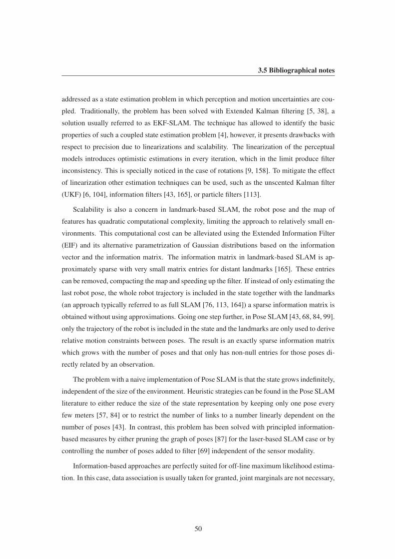
3.5 Bibliographical notes
addressed as a state estimation problem in which perception and motion uncertainties are cou-
pled. Traditionally, the problem has been solved with Extended Kalman filtering [5, 38], a
solution usually referred to as EKF-SLAM. The technique has allowed to identify the basic
properties of such a coupled state estimation problem [4], however, it presents drawbacks with
respect to precision due to linearizations and scalability. The linearization of the perceptual
models introduces optimistic estimations in every iteration, which in the limit produce filter
inconsistency. This is specially noticed in the case of rotations [9, 158]. To mitigate the effect
of linearization other estimation techniques can be used, such as the unscented Kalman filter
(UKF) [6, 104], information filters [43, 165], or particle filters [113].
Scalability is also a concern in landmark-based SLAM, the robot pose and the map of
features has quadratic computational complexity, limiting the approach to relatively small en-
vironments. This computational cost can be alleviated using the Extended Information Filter
(EIF) and its alternative parametrization of Gaussian distributions based on the information
vector and the information matrix. The information matrix in landmark-based SLAM is ap-
proximately sparse with very small matrix entries for distant landmarks [165]. These entries
can be removed, compacting the map and speeding up the filter. If instead of only estimating the
last robot pose, the whole robot trajectory is included in the state together with the landmarks
(an approach typically referred to as full SLAM [76, 113, 164]) a sparse information matrix is
obtained without using approximations. Going one step further, in Pose SLAM [43, 68, 84, 99].
only the trajectory of the robot is included in the state and the landmarks are only used to derive
relative motion constraints between poses. The result is an exactly sparse information matrix
which grows with the number of poses and that only has non-null entries for those poses di-
rectly related by an observation.
The problemwith a naive implementation of Pose SLAM is that the state grows indefinitely,
independent of the size of the environment. Heuristic strategies can be found in the Pose SLAM
literature to either reduce the size of the state representation by keeping only one pose every
few meters [57, 84] or to restrict the number of links to a number linearly dependent on the
number of poses [43]. In contrast, this problem has been solved with principled information-
based measures by either pruning the graph of poses [87] for the laser-based SLAM case or by
controlling the number of poses added to filter [69] independent of the sensor modality.
Information-based approaches are perfectly suited for off-line maximum likelihood estima-
tion. In this case, data association is usually taken for granted, joint marginals are not necessary,
50

3.5 Bibliographical notes
and the estimate only includes the state mean, which is iteratively approximated representing
the relative displacement between poses as quadratic constraints [52, 57, 99, 128] or by factor-
izing the sparse information matrix [35]. Moreover, besides on-line approaches to Pose SLAM
relying on filtering [43, 68], we can find variants of the batch methods [76] as well.
Data association is another issue in SLAM and it is specially difficult in environments
where landmarks are difficult to distinguish as well as in environments with aliasing. An im-
portant advance in the data association problemwas the concept of batch gating, where multiple
associations are considered simultaneously [9, 118]. Furthermore, the standard formulation of
the EKF-SLAM solution is especially fragile to incorrect association of observations to land-
marks [23], and in order to validate the history of data association, temporal landmark quality
measures and a temporal landmark quality test were proposed in [3]. These quality measures
allow longer mapping sequences through the elimination of inconsistent observations. This
removal of weak landmarks from the state vector and state covariance matrix did not violate
the convergence properties of SLAM. Other ways to perform reliable data association include
other sensing modalities, such as vision. For instance, appearance signatures [32, 119] are
useful to predict a possible association, such as closing a loop. Another alternative is to ex-
ploit the filter information to constrain the search for sensory matches only to few neighboring
poses [43, 68, 69]. For consistent estimates, this latter option is more efficient and less affected
by perceptual aliasing.
Another problem in SLAM is that of the environment representation. Early works in
SLAM, usually in indoor settings, modeled the world as a set of two dimensional landmarks,
however, this representation is of little help in more complex and unstructured environments.
Diverse types of representation can be used. As noted in [175], according to the reference frame
to which estimates are linked, we can distinguish between world-centric and sensor-centric rep-
resentations. Moreover, if the world is described by a qualitative or geometrical description we
can distinguish between topological and geometrical maps, respectively.
Geometrical representations in SLAM are the most popular. They can be further classified
by the degrees-of-freedom (DOF) of the robot pose and the dimensionality of sensor data,
as noted in [124], yielding four typical representations: planar maps with a 3 DOF SLAM,
planar or slice-wise maps with a 6 DOF SLAM, 3D maps with a 3 DOF SLAM, and 3D maps
with 6 DOF SLAM. This latter solution has received special attention. In [124] this problem
is addressed by a scan alignment approach for 3D scans gathered by a rotating laser scanner
51

3.5 Bibliographical notes
sensor, where the alignment of two scans is done mainly by improvements to the basic ICP
algorithm proposed in [15]. For the same type of solution and with a similar a sensor setting, a
delayed-state framework with an Extended Kalman Filter was proposed in [31], and eventually
a scalable version with only informative links and poses was presented in [172] using the Pose
SLAM approach in 6 DOF.
The approaches so far discussed are passive in the sense that the robot only estimates the
model of the environment, but without taking any decisions on its trajectory. Another challenge
in SLAM is to compute the appropriate robot actions to reduce the uncertainty about its own
localization and the map, while at the same time optimizing coverage [96, 147, 172, 177].
Many issues still remain to be solved, e.g. dynamic environments, multirobot SLAM, life-
long SLAM techniques. Another related issue, usually neglected in SLAM implementations, is
to endow the robot the ability to actually use the maps it builds, just after it builds them, which
might bring closer the possibility of long-term autonomous existence. This thesis contributes
on this venue with a path planning under uncertainty using Pose SLAM maps. Chapter 4 will
introduce this problem, including a bibliographical review on the related work to this issue as
well. Furthermore, another contribution of this thesis is an active Pose SLAM approach, which
will be introduced in Chapter 5, together with a review of the related work that will complement
this section.
52

Chapter 4
Path planning in belief space with
Pose SLAM
The probabilistic belief networks that result from standard feature-based simultaneous local-
ization and map building methods cannot be directly used to plan trajectories. The reason is
that these methods produce a sparse graph of landmark estimates and their probabilistic rela-
tions, which is of little value to find collision free paths for navigation. These graphs can be
enriched with obstacle or traversability related information, but at the expense of an increase
in complexity. Moreover, the resulting planning methods typically do not exploit the sources
of uncertainty encoded in the maps. In contrast, we argue in this Chapter that Pose SLAM
graphs can be directly used as belief roadmaps [62, 134] and, thus, used for path planning un-
der uncertainty. The method we present in this Chapter devises optimal navigation strategies
by searching for the path in the pose graph with the lowest accumulated robot pose uncertainty,
i.e., the most reliable path to the goal.
Aside from applications such as the reconstruction of archaeological sites [44] or the in-
spection of dangerous areas [167], the final objective for an autonomous robot is not to build a
map of the environment, but to use this map for navigation. Whereas in the seminal approaches
to SLAM [151] only few tens of landmarks could be managed, state of the art approaches can
now efficiently manage thousands of landmarks [53, 83, 166] and build maps over several
kilometers [146]. However, for efficiency reasons, most SLAM algorithms represent the en-
vironment using a sparse set of features. Unfortunately, this representation cannot be directly
used for collision-free path planning since it does not provide much information about which
routes in the map have been previously traversed safely, or about the nature of the obstacles
53

it represents. Those sparse models could be somehow enriched with obstacle or traversabil-
ity related information [59, 121, 137], but at the expense of an increase in complexity. For
instance, the traversability map shown in Chapter 3 requires to further process the volumetric
map obtained with Pose SLAM.
The problem of finding paths to reach distant locations is addressed in the motion planning
literature. However, the research in motion planning typically assumes deterministic setups
where a perfect model of the environment is available and where the configuration of the robot
is perfectly known too. The most successful methods are based on randomized sampling [78,
91], in which collision-free configurations are stochastically drawn and where, if possible,
neighbor samples are connected forming a roadmap. This roadmap is later used to find a
path between any two given configurations. Some approaches have addressed the problem of
optimizing the quality of this path, mainly focusing on reducing the path length [77, 136].
Some extensions have been introduced to deal with uncertainties in the model of the en-
vironment [112], in the robot configuration [129], in the effect of robot actions [1], or in the
effect of actions and measurements [18]. The extension that best matches the stochastic na-
ture of SLAM is the Belief Roadmap (BRM) [62, 134]. In this approach, the edges defining
the roadmap include information about the uncertainty change when traversing such an edge.
However, the main drawback of the BRM is that it still assumes a known model of the en-
vironment, which is in general not available in real applications. In this thesis, we aim to
overcome the limitation of BRMs noting that the map generated by Pose SLAM [69], or any
other delayed-state SLAM method [43, 84, 99], can be directly used as a belief roadmap (see
Fig. 4.1).
In a semi-autonomous scenario where a human initially drives the robot through a set of in-
terest way points, the outcome of Pose SLAM is a graph of obstacle-free paths in the area where
the robot has been operated. Using this graph for navigation allows to have an infrastructure-
free automated guided vehicle, as those widely used for surveillance, for material distribution in
factories, or for drug delivery in hospitals [108, 187]. An added advantage is that Pose SLAM
is agnostic with respect to the sensor modalities used, which facilitates its application in dif-
ferent environments and robots, and the paths stored in the map satisfy constraints not easy to
model in the robot controller, such as the existence of restricted regions, or the right of way
along paths. Deviations from these paths might result in an inconvenience for other operations
carried out in the factory or hospital. Thus, a robot that can adequately choose the correct path
54

(a)
−10 −5 0 5 10
−8
−6
−4
−2
0
2
4
6
8
X(m)
Y(m
)
START
GOAL
(b)
−10 −5 0 5
−8
−6
−4
−2
0
2
4
6
8
X(m)
Y(m
)
START
GOAL
(c)
Figure 4.1: Path planning using the map generated by the Pose SLAM algorithm. (a) The
Pose SLAM map. The red dots and lines represent the estimated trajectory, and the green lines
indicate loop closure constraints established by registering sensor readings at different poses.
(b) A plan in configuration space would produce the shortest path to the goal. At one point
during path execution, sensor registration fails and the robot gets lost. This happens when the
robot is outside the sensor registration area for a given waypoint in the tracked trajectory. The
areas around each pose where registration is possible are represented by rectangles. (c) A plan
in belief space produces the minimum uncertainty path to the goal. Plans with low uncertainty
have higher probability of success.
55

3 4 5 6 7 8
3.5
4
4.5
5
5.5
6
6.5
7
7.5
X(m)
Y(m
)
Figure 4.2: Zoomed view of a region along the shortest path in Fig. 4.1 where the robot gets
lost. Bad localization on this path leads the robot to deviate from the next waypoint, producing
failed sensor registration. The rectangles indicate the areas where sensor registration is reliable
(shown in black for the poses in the map and in red for the poses in the executed trajectory),
the green lines represent sensor registration links between poses in the executed trajectory and
those in the map, and the blue lines and ellipses represent the localization estimates for the
executed trajectory.
from a set of previously traversed ones, or their combination, is desirable for such applications.
However, in those scenarios, the use of a robot is only practical if it is able to navigate without
becoming lost, i.e., without requiring the intervention of the operator. The research reported in
this Chapter addresses this issue, providing the safest path from one waypoint to another.
In most cases, any two poses are connected by different paths, and navigating through
one or the other would entail different probabilities of becoming lost. A path through areas
where sensory data is not reliable means higher risk of deviating from the path to follow during
execution (see Fig. 4.2). In this Chapter, we show that, using Pose SLAM, we can plan in the
belief space to obtain paths that take into account the uncertainties along the path. The key idea
behind our method is that, in Pose SLAM, highly informative areas of the environment result
in poses in the graph with low uncertainty. Thus, paths through safer areas in the sense of being
reliably localized can be selected considering only the pre-computed uncertainties encoded in
the graph.
From the point of view of SLAM, this method constitutes a step forward to actually use
56

4.1 Path planning with Pose SLAM
the output of the mapping process for path planning. From the point of view of motion plan-
ning, this approach contributes with a method to generate belief roadmaps without resorting to
stochastic sampling on a pre-defined environment model.
The rest of the Chapter details the proposed approach to perform path planning. As we
mentioned, this method reinterprets the Pose SLAM map as a set of samples in belief space
and, in Section 4.1 we describe how to plan using a roadmap defined on these samples. Next,
Section 4.2 presents the planning algorithm. In Section 4.3, this new planning approach is
tested with datasets and a real world experiment. Finally, Section 4.4 shows the related work
to our approach.
4.1 Path planning with Pose SLAM
We are in the quest for a path p = r1:T that would drive the robot from its current configuration
st = r1 to a goal configuration g = rT , that, for the applications considered in this thesis, is
always included in the Pose SLAM graph. In this quest, we assume that the robot is equipped
with a local planner able to drive the robot to nearby configurations.
Moreover, we assume maximum likelihood actions and measurements, as it is usual when
planning in belief space [132]. With this, the mean estimate after a sequence of controls will lie
at the mean of a node in the graph and the observation previously obtained at that position will
be repeated. In consequence, the proposed planning approach only needs to consider poses in
the graph, which are guaranteed to be collision free.
Given that candidate paths lie on the top of this graph, after path execution the final robot
uncertainty will be close to the original marginal at that node. Thus, a cost function that only
evaluates the belief state at the goal is unsuitable and we are interested instead in determining
reliable paths, i.e., paths where the robot has low probability of becoming lost. Herein, we
assume that the probability of becoming lost is directly related with the increments in the
uncertainty in the robot positioning since uncertainty decrements can only result in a better
track of the path.
We propose to achieve this objective in four stages. First, we increase the connectivity of
the Pose SLAM graph so that paths combining different exploration sequences can be con-
sidered. Next, we propose a principled way to evaluate the uncertainty of transitions between
nodes. Then, we use this uncertainty measure to define the cost of a path as its mechanical
57
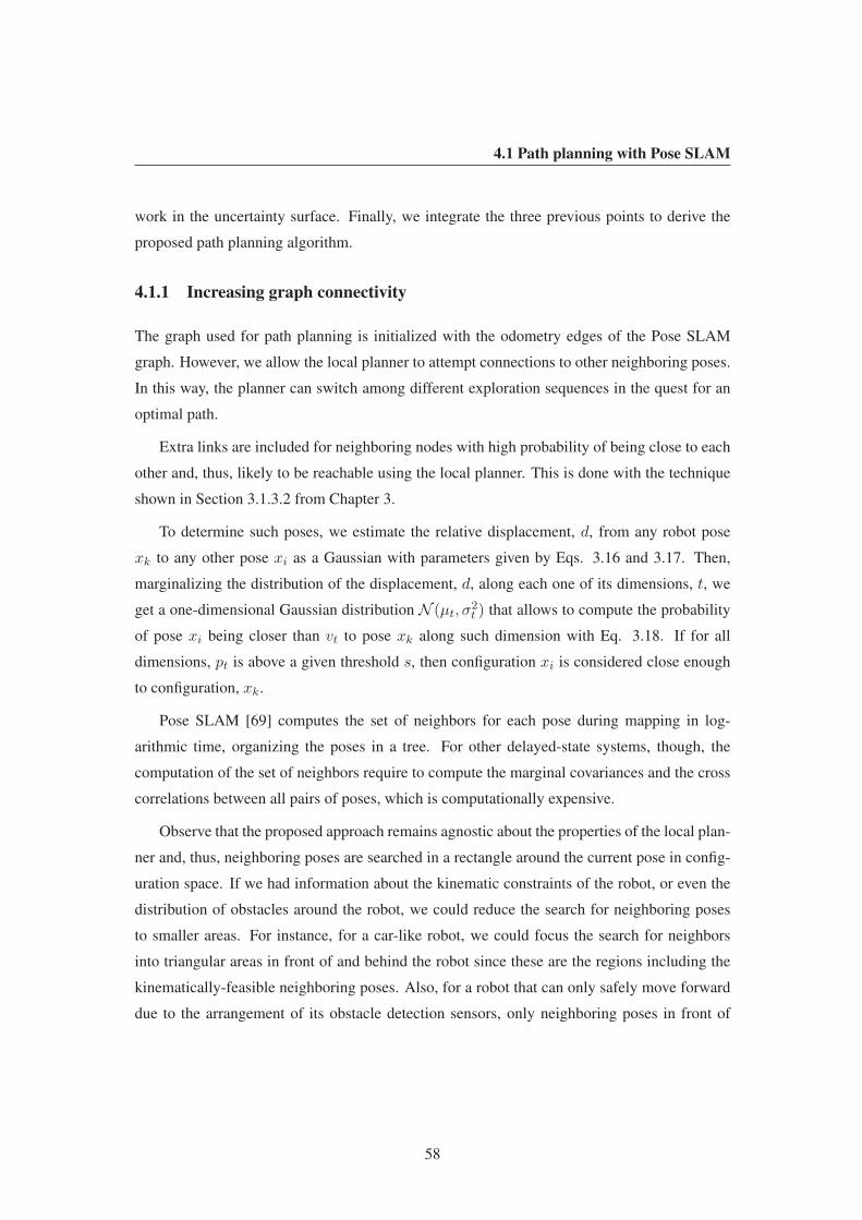
4.1 Path planning with Pose SLAM
work in the uncertainty surface. Finally, we integrate the three previous points to derive the
proposed path planning algorithm.
4.1.1 Increasing graph connectivity
The graph used for path planning is initialized with the odometry edges of the Pose SLAM
graph. However, we allow the local planner to attempt connections to other neighboring poses.
In this way, the planner can switch among different exploration sequences in the quest for an
optimal path.
Extra links are included for neighboring nodes with high probability of being close to each
other and, thus, likely to be reachable using the local planner. This is done with the technique
shown in Section 3.1.3.2 from Chapter 3.
To determine such poses, we estimate the relative displacement, d, from any robot pose
xk to any other pose xi as a Gaussian with parameters given by Eqs. 3.16 and 3.17. Then,
marginalizing the distribution of the displacement, d, along each one of its dimensions, t, we
get a one-dimensional Gaussian distribution N (µt, σ2t ) that allows to compute the probability
of pose xi being closer than vt to pose xk along such dimension with Eq. 3.18. If for all
dimensions, pt is above a given threshold s, then configuration xi is considered close enough
to configuration, xk.
Pose SLAM [69] computes the set of neighbors for each pose during mapping in log-
arithmic time, organizing the poses in a tree. For other delayed-state systems, though, the
computation of the set of neighbors require to compute the marginal covariances and the cross
correlations between all pairs of poses, which is computationally expensive.
Observe that the proposed approach remains agnostic about the properties of the local plan-
ner and, thus, neighboring poses are searched in a rectangle around the current pose in config-
uration space. If we had information about the kinematic constraints of the robot, or even the
distribution of obstacles around the robot, we could reduce the search for neighboring poses
to smaller areas. For instance, for a car-like robot, we could focus the search for neighbors
into triangular areas in front of and behind the robot since these are the regions including the
kinematically-feasible neighboring poses. Also, for a robot that can only safely move forward
due to the arrangement of its obstacle detection sensors, only neighboring poses in front of
58

4.1 Path planning with Pose SLAM
the robot need to be detected. In any case, the size of the area where to look for neighbors is
limited by the accuracy of the local planner, which typically relies in odometry readings.
Independently of the location and size of the area used to search for neighbors, an edge
is added to the path planning graph only if the kinematic constraints enforced by the local
planner allow to reach the nearby node. Despite this verification, the local path might still
result unfeasible during path execution, mainly due to the presence of obstacles. Then, the
problematic edge can be removed from the graph and a re-planning process can be triggered.
4.1.2 Uncertainty of a path step
To track a path within the pose SLAM map, the robot departs from an initial pose estimate
and predicts a new estimate taking into account the relative motion constraint between two
consecutive nodes in the path. Such a tracker would update this new estimate registering current
sensor readings to those stored in the corresponding map node. Thus, every pair of poses in a
planned path, say rk−1 and rk, would match two poses in the Pose SLAM graph, say xi and
xj . The command uk that drives the robot from rk−1 to rk and the associated motion noiseΣu
are provided by the local planner. Since, during the planning process the actual sensor readings
are not available, the update of this estimate is made assuming that at the end of the step from
rk−1 to rk, rk and xj will be coincident and, thus, zkj = rk − xj ∼ N (0,Σjj) where Σjj is
the marginal covariance of the pose xj .
To evaluate the change in uncertainty introduced in the motion from rk−1 to rk, we must
look at the conditional distribution p(rk|rk−1, uk, zkj) that is obtained from the estimation of
the joint state (rk−1, rk). This estimation can be obtained using, for instance, an EKF [169], as
we show next.
The cost of traversing a link from node rk−1 to node rk is proportional to the conditional
entropy at node j given full confidence about node i, H(rk|rk−1), which for Gaussians is
proportional to
H(rk|rk−1) ∝ |Σk,k − Σk,k−1Σ−1k−1,k−1Σk−1,k|, (4.1)
where the marginals and cross-correlations are extracted from Σ, the covariance of the com-
pound localization estimate (rk−1, rk). Equation 4.1 is a measure of the robot’s ability to safely
track its position during path execution. To compute both marginals and cross correlation terms
in Eq. 4.1 we need to track localization estimates of the previous and current robot poses xi
59

4.1 Path planning with Pose SLAM
and xj . To this end, the compound localization estimate (xi, xj) can be computed with the
Extended Kalman Filter (EKF), with the particularity that every EKF update is given by sensor
registration with the Pose SLAM graph at node j, taking into account its marginal covariance
Σjj .
Nevertheless, going a step further, this uncertainty can be more elegantly evaluated using
an EIF instead. With an EIF, (rk−1, rk) is estimated as N−1(η, Λ) and in the prediction step
the joint information matrix is updated as [43]
[
Λk−1k−1 + FΣ−1u F⊤ −F⊤Σ−1
u
−Σ−1u F Σ−1
u
]
, (4.2)
with F the Jacobian of f with respect to rk−1 evaluated at the mean, and where Λk−1k−1 is
obtained marginalizing from the previous Λ. In the correction step the measurement zkj is
used to update the information matrix as
Λ =
[
Λk−1k−1 + FΣ−1u F⊤ −F⊤Σ−1
u
−Σ−1u F Σ−1
u +Σ−1jj
]
. (4.3)
With this, the uncertainty of rk given full confidence about rk−1 can be evaluated as
H(rk|rk−1) ∝1
|Λk|k−1|, (4.4)
where Λk|k−1 is the information matrix for the conditional p(rk|rk−1, uk, zkj) obtained from
Λ.
Fortunately enough, conditioning in information form is dual to marginalization in covari-
ance form, which saves us from computing the state covariance of the tracker and the Schur
complement to condition the covariance, as done in Eq. 4.1. Thus, using the EIF estimation,
Eq. (4.4) simply evaluates to
Uk =1
|Σ−1u +Σ−1
jj |. (4.5)
We can safely assume Σu to be non-degenerate and, thus, the determinant in Eq. (4.5) would
never be null and Uk will be always well-defined. Note that we use a measure of uncertainty
change derived from the determinant of the covariance matrix which is related to the entropy
of p(rk|rk−1, uk, zkj), and ultimately, to the uncertainty hyperellipsoid defined by this matrix.
A trace-based uncertainty measure [134] can be used as well, without affecting the overall
planning algorithm.
60

4.1 Path planning with Pose SLAM
Note that this measure of uncertainty change is computed independently of the estimation
of the robot pose at that step and, thus, this formulation saves us from actually implementing the
EIF to track the path. This does not imply that the robot must have an identical belief to a pre-
existing node in the optimized Pose SLAM graph. What it implies is that the computation of the
information gain is independent of the current belief, as long as maximum likelihood actions
and measurements are considered. This is especially relevant to allow planning with different
initial beliefs. Moreover, as long as the graph does not change, the uncertainty measure for all
transitions can be precomputed from the Pose SLAM graph and re-used to plan different paths.
This is similar to what is done in [134], factorizing the covariance update, but simplified thanks
to the use of the information form.
4.1.3 Minimum uncertainty along a path
Next, we propose a cost function that considers cumulative relative uncertainty during local-
ization. In principle, only increments in uncertainty are problematic for the quality of the
localization since any decrement in uncertainty can only result in a better estimate. Therefore,
finding paths that accumulate the least uncertainty can be seen as searching for a path of mini-
mal mechanical work [72] in an uncertainty surface [150] over the space of robot poses, where
the uncertainty of a path step is computed using the criterion described in Section 4.1.2.
Given a discrete path p = r1:T , we define its mechanical work in the uncertainty surface as
the sum of positive increments of individual step costs
W (r1:T ) =
T∑
k=2
∆U+k , (4.6)
with
∆U+k =
∆Uk ∆Uk > 0,
0 ∆Uk ≤ 0,(4.7)
and
∆Uk = Uk − Uk−1 (4.8)
and where, by convention, U1 = 0, to include the uncertainty of the first step of the path in
W . Note that, the initial uncertainty of the robot is not included inW since it would result in a
constant offset for the cost of all alternative paths. Moreover, since the costs are non-negative,
there is always an acyclic minimum cost path to each reachable node in the map.
61

4.2 The Pose SLAM path planning algorithm
This strategy prefers short paths with possibly steep uncertainty changes over much longer
paths with gentle oscillations of uncertainty, thus avoiding the accumulation of small chances
of becoming lost over large trajectories. In this way, the proposed strategy is a mechanism that
adequately balances path length with uncertainty change.
4.2 The Pose SLAM path planning algorithm
To find the optimal path, Dijkstra’s algorithm is implemented with the cost function defined in
Section 4.1.3. It is formally described in Algorithm 1. It implements a minimum uncertainty
path search among paths tracked on the poses in a Pose SLAM graph. The algorithm takes as
inputs the Pose SLAM graphM and the goal pose, g, which is assumed inM . Should this not
be the case, the closest pose in the graph to g (in configuration space) is used as a goal. We
first initialize a setQ with all the nodes in the graph (Line 1) and establish an initial costW for
the path to each node (Line 3) and a fake predecessor V for each node (Line 4). Then, the cost
to reach the starting configuration is set to 0 (Lines 5 to 7). At this point the algorithm enters
in a loop until the goal is reached or the reachable region from the start configuration is fully
explored (Lines 8 to 26). At each iteration of the loop, we extract the node i with minimum
cost from Q (Line 9). If this is not the goal (Line 10), we perform breadth first search on the
neighbor nodes to i (Line 11). The neighboring nodes are determined using the procedure given
in Section 4.1.1 that takes into account the uncertainty in the pose estimates. For each one of
the possible transitions to neighbors, we use the local planner to determine if the transition
is possible and to compute the expected motion uncertainty (Line 13). Using this uncertainty
and the marginal covariance for the target pose (Line 15) we compute the step uncertainty as
described in Section 4.1.2 (Line 16). Then, Line 17 computes the uncertainty increment for a
motion from node i to node j. If this increment is positive, it is added to the path cost (Line 19).
Otherwise, this step does not contribute to the overall path cost. If the new path to j is lower
than the best known until that moment, the cost to reach j is updated (Line 23), we set i as the
predecessor of j (Line 24), and we store the cost for the path to the node (Line 25). In the case
of paths with equal cost, shorter ones are preferred and, since the costs of individual steps are
non-negative, the considered paths never include cycles. If the goal is reached, the minimum
uncertainty path to the goal is reconstructed using the chains to predecessor nodes stored in V
(Lines 30 to 32). If the goal is determined to be non-reachable from the start configuration, an
empty path is returned.
62

4.2 The Pose SLAM path planning algorithm
Algorithm 1: Path planning with Pose SLAM.
PoseSLAMPathPlanning(M ,g)
input :M : The graph computed by Pose SLAM.
g: The goal pose.output: p: Minimum uncertainty path to g.
Q← POSES(M)1
forall n ∈ Q do2
W [n]←∞3
V [n]← 04
st ← CURRENTPOSE(M)5
W [st]← 06
U [st]← 07
repeat8
i← EXTRACTMIN(Q,W )9
if i 6= g andW [i] 6=∞ then10
N ← NEIGHBORS(M, i)11
forall j ∈ N do12
(u,Σu)← LOCALPLANNER(xi,xj)13
if u 6= ∅ then14
Σjj ← MARGINALCOVARIANCE(M, j)15
U = 1/|Σ−1
u + Σ−1
jj |16
∆U = U − U [i]17
if∆U > 0 then18
W ′ =W [i] + ∆U19
else20
W ′ =W [i]21
ifW ′ < W [j] then22
W [j]←W ′23
V [j]← i24
U [j]← U25
until i = g orW [i] =∞ or Q = ∅ ;26
p← ∅27
if i = g then28
c← g29
while c 6= 0 do30
p← c ∪ p31
c← V [c]32
RETURN p33
Without considering the cost of recovering the marginal covariances, the asymptotic cost of
the algorithm isO(e log2 n)with e the number of edges in the graph (i.e., the number of neigh-
boring pose pairs) and n the number of nodes in the graph. This cost assumes that the nodes
63

4.3 Experimental results
in Q are organized into a heap where the extraction of the minimum element is constant time
and the update of the cost of an element is logarithmic. Moreover, it also assumes that poses
are organized into a tree so that neighboring poses can be determined logarithmically [69]. If
this search is performed linearly the cost increases to O(e n log n).
Note that, when planning we do not need to maintain a localization estimate, but still we
need to simulate registration with the map, for which the diagonal blocks of the covariance
matrix are needed (Line 16). When using the Pose SLAM algorithm [69], these diagonal blocks
are directly available [70], but this is not the case in other approaches [43, 84, 99]. In these
cases, the most efficient way to compute the marginals is to invert the whole information matrix
before starting to plan. One can efficiently invert it taking advantage of its sparsity using, for
instance, sparse supernodal Cholesky decomposition [26]. For large-scale problems, however,
this strategy becomes prohibitively expensive and we have to resort to approximations of the
marginal covariances obtained using, for instance, Markov blankets [165].
Finally, should the map change significantly during path execution (i.e., a new highly in-
formative loop closure is found), the Pose SLAM algorithm performs a full state update and
re-planning is enforced.
4.3 Experimental results
In order to evaluate the planning strategy presented in this Chapter we show results with four
data sets and with a real robot navigation experiment. The results with the data sets were
obtained with a Matlab implementation running on an Intel Core2 Quad system at 3 GHz
with 4 GB of memory. For the real robot navigation experiment, the system was implemented
using the Robot Operating System (ROS) [135] on our 4-wheel robot Teo, a Segway RMP400
platform.
4.3.1 Synthetic dataset
In the first experiment, we simulate a robot moving over a given trajectory with several loops. In
the simulation, the motion of the robot is measured with an odometric sensor whose error is 5%
of the displacement in x and y, and 0.0175 rad in orientation. A second sensor is simulated to
establish links between any two poses closer than±1.25m in x,±0.75m in y, and±0.26 rad inorientation, with noise covariance Σz = diag(0.2m,0.2m,0.009 rad)2. The initial uncertainty
64

4.3 Experimental results
0 5 10 15 20 25 30 35 40 450
0.2
0.4
0.6
0.8
1
1.2
1.4
1.6
1.8x 10
−6
Path length(m)
Accum
ula
ted C
ost
Minimum Uncertainty Path
Shortest Path
Figure 4.3: Accumulated cost along the shortest (red) and minimum uncertainty (blue) paths
in the simulated experiment.
in the robot pose is set to Σ0 = diag(0.1m, 0.1m, 0.09 rad)2. Nearby poses are detected with
a very permissive s = 0.1. With such value of s we avoid missing any neighbor. Finally, the
minimum information gain, γ is set to 3 nats.
Figure 4.1(a) shows the final map as estimated by the Pose SLAM algorithm. The shad-
owed area indicates harsher navigation conditions with odometry and loop closure errors in-
creased by a factor of 8. This noisier area simulates a part of the environment where constraints
between poses are harder to establish.
After building the map using Pose SLAM we planned a path to a particular goal selected
from the nodes in the map. Fig. 4.1(b) shows the trajectory to the goal using a shortest path
criterion, and Fig. 4.1(c) shows the trajectory obtained when using the minimum uncertainty
criterion introduced in Section 4.1.3, which avoids the noisier area in the environment.
Fig. 4.3 shows a plot of the accumulated cost along the two trajectories. The accumulated
uncertainty of the shortest path is significantly larger than that of the minimum uncertainty
path. Therefore, following this second trajectory there is increased guarantee that the robot
will be better localized all along the path and will less likely get into trouble, for instance,
of getting lost. This is verified in Fig. 4.4 that shows a Monte Carlo realization of the this
experiment with 100 runs. Navigation through the shortest path reached the goal only 45% of
65

4.3 Experimental results
−10 −5 0 5 10
−8
−6
−4
−2
0
2
4
6
8
X(m)
Y(m
)
START
GOAL
Figure 4.4: Monte Carlo realization of the simulated experiment. The minimum uncertainty
path guarantees path completion during localization as indicated by the blue trajectories. The
red dots indicate on the other hand, the points where the robot gets lost due to a missed sensor
registration, while executing the shortest path.
the times due to failed sensor registration along the path, whereas navigating over the minimum
uncertainty path always reached the final destination since the trajectory avoids the noisier area
in the environment.
4.3.2 Indoor dataset
To test the performance of the algorithm on an indoor data set we choose the data collected
at the Intel Research Lab building in Seattle [66]. The dataset includes 26915 odometry read-
ings and 13631 laser scans. The laser readings were used to generate scan-based odome-
try and to assert loop closures, by aligning them using an incremental closest point (ICP)
scan matching algorithm [99]. In this case, only links between poses closer than ±1m in x
and y, and ±0.35 rad in orientation were considered reliable. These are also the thresholds
used to determine neighboring poses when planning with s = 0.1. The robot odometry and
the relative motion computed from laser scan matches were modeled with noise covariances
66

4.3 Experimental results
(a) Pose SLAM map.
−10 −5 0 5 10 15
−20
−15
−10
−5
0
X(m)
Y(m
)
START
GOAL
(b) Plan in configuration space.
−10 −5 0 5 10 15
−20
−15
−10
−5
0
X(m)
Y(m
)
START
GOAL
(c) Plan in belief space.
Figure 4.5: Path planning over the Intel dataset. (a) Pose SLAMmap built with encoder odom-
etry and laser scans. The blue arrow indicates the final pose of the robot and the black ellipse
the associated covariance at a 95% confidence level. (b) Planning in configuration space we
obtain the shortest path to the goal on the underlying Pose SLAM graph. (c) Planning in belief
space we obtain the minimum uncertainty path to the goal.
67

4.3 Experimental results
0 5 10 15 20 25 30 35 400
0.1
0.2
0.3
0.4
0.5
0.6
0.7
0.8
0.9
1x 10
−6
Path length(m)
Accum
ula
ted C
ost
Minimum Uncertainty Path
Shortest Path
Figure 4.6: Accumulated cost versus the path length for the shortest path (red) and minimum
uncertainty path (blue) in the Intel experiment.
Σu = diag(0.05m, 0.05m, 0.03 rad)2 and Σz = diag(0.05m, 0.05m, 0.009 rad)2, respec-
tively and the minimum information gain was γ =4.5 nats. Fig. 4.5(a) shows the path estimated
by Pose SLAM together with the laser scans associated to each of the stored poses in light gray.
This map is the departing point of the planning algorithm and the goal is to connect two
poses on opposite sides of the building. Frames (b) and (c) in Fig. 4.5 show the shortest and
minimum-uncertainty paths between the two poses. The apparent overshoot of the shortest path
to the goal is due to the fact that the robot has to execute a 180 deg turn at the end of the path
to align with the goal since sudden changes in orientations are not allowed by the kinematic
constraints assumed for the robot. This rotation is only possible few meters away of the goal,
in front of a door where many poses with the robot at different orientations accumulate.
Figure 4.6 shows the accumulated cost along the two paths. We can note that the accu-
mulated uncertainty of the shortest path is larger than that for the minimum uncertainty path.
Therefore, following this second path the robot is better localized all the time at the cost of
following a slightly larger path.
To test the efficiency of the method, Fig. 4.7 shows the execution time and memory foot-
print for planning as a function of problem size, varying the number of poses in the Intel map.
Since the most expensive step of the algorithm is the recovery of the marginal covariances,
68

4.3 Experimental results
100 200 300 400 500 600 7000
5
10
15
20
25
Number of Poses
Tim
e (
s)
Whole cov. matrix (Planning time)
Whole cov. matrix (Recovering time)
Column−wise (Planning time)
Column−wise (Recovering time)
(a) Execution time
100 200 300 400 500 600 7000
0.5
1
1.5
2
2.5
3
3.5
4
4.5
Number of Poses
Mem
ory
(M
b)
Whole cov. matrix
Column−wise
(b) Memory footprint
Figure 4.7: Plots of execution time and memory footprint when planning with different subsets
of the Intel map and employing two different strategies to recover marginals. (a) Execution time
needed to recover only the marginals (continuous line) and for the whole planning algorithm
(dashed line). (b) Memory footprint for marginal recovery.
we applied two different strategies to recover them: recovering the whole Σ and recovering it
column-wise as needed during planning. The continuous lines in Fig. 4.7(a) show the execu-
tion time needed to recover the marginals as a function of problem size, whereas the dashed
lines show the execution time of the whole planning algorithm also as a function of problem
69

4.3 Experimental results
−160 −140 −120 −100 −80 −60 −40 −20 0 20 40−140
−120
−100
−80
−60
−40
−20
0
20
X(m)
Y(m
)START
GOAL
(a) Plan in configuration space
−160 −140 −120 −100 −80 −60 −40 −20 0 20 40−140
−120
−100
−80
−60
−40
−20
0
20
X(m)
Y(m
)
GOAL
START
(b) Plan in belief space.
Figure 4.8: Path planning over the Manhattan dataset. (a) Planning in configuration space we
obtain the shortest path to the goal on the underlying Pose SLAM graph. (b) Planning in belief
space we obtain the minimum uncertainty path to the goal.
70

4.3 Experimental results
0 50 100 150 200 250 300 350 400 4500
0.2
0.4
0.6
0.8
1
1.2x 10
−8
Path length(m)
Accum
ula
ted C
ost
Minimum Uncertainty Path
Shortest Path
Figure 4.9: Accumulated cost along the shortest (red) and minimum uncertainty (blue) path in
the Manhattan experiment.
size. The figure shows that recovering the whole matrix is computationally more efficient at
the expense of increased memory space. On the contrary, on-the-fly computation of matrix
columns results in repeated computations slowing down planner performance. The execution
cost of re-planning when a graph edge is found to be non-traversable is reduced to the differ-
ence between the continuous and the dashed lines in Fig. 4.7(a) since the map does not change
and, thus, the marginal covariances do not need to be re-computed.
4.3.3 Large scale dataset
To demonstrate scalability, we tested our approach with a much larger map, for which mem-
ory space is a constraint. To this end, we planned paths using the simulated Manhattan data
set [128] that includes over 10000 poses. In this experiment, noise covariances for robot
odometry and the relative-pose measurements were set to Σu = Σz = diag(0.05m, 0.05m,
0.03 rad)2, the threshold to detect neighboring poses was s = 0.1 searching in a rectangle
around the robot given by ±8m in x, ±8m in y, and ±1 rad in orientation. We only incor-
porated links between poses with an information gain above γ =9 nats.
Figure 4.8 shows the shortest and minimum-uncertainty paths between the chosen start and
goal poses, with the corresponding accumulated costs shown in Fig. 4.9.
71

4.3 Experimental results
−80 −70 −60 −50 −40 −30 −20 −10 0 10
−60
−50
−40
−30
−20
−10
0
10
20
30
40
X(m)
Y(m
)
GOAL
START
(a) Plan in configuration space.
−80 −70 −60 −50 −40 −30 −20 −10 0 10
−60
−50
−40
−30
−20
−10
0
10
20
30
40
X(m)
Y(m
)
START
GOAL
(b) Full covariance recovery.
−80 −70 −60 −50 −40 −30 −20 −10 0 10
−60
−50
−40
−30
−20
−10
0
10
20
30
40
X(m)
Y(m
)
GOAL
START
(c) Markov blanket approximation.
Figure 4.10: Path planning over a section of the Manhattan dataset. (a) Planning in config-
uration space we obtain the shortest path to the goal on the underlying Pose SLAM graph.
(b) Planning in belief space we obtain the minimum uncertainty path to the goal. (c) A mini-
mum uncertainty path to the goal computed when the marginal covariances are recovered with
Markov blankets.
With this dataset, full matrix recovery is not feasible with the computing resources used,
and column-wise marginal computation is impractically slow. Therefore, marginal covariances
are approximated using Markov blankets [165]. In this method the marginal covariance for
a given pose is approximated considering only the subgraph of poses directly connected to it,
which is typically small. As expected, the cost of the minimum uncertainty path obtained using
72

4.3 Experimental results
50 100 150 200 250 300 350
0.7
0.8
0.9
1
1.1
1.2
1.3
1.4
1.5
x 10−8
Path length (m)
Accu
mu
late
d c
ost
Shortest Path
Minimum Uncertainty Path
Minimum Uncertainty Path (Markov Blankets)
Figure 4.11: Accumulated cost along the shortest (red) and along the minimum uncertainty
path computed with exact marginal covariances (blue) and with Markov blankets (black).
Markov blankets is significantly better than that of shortest path, with only a marginal increase
in path length. The planning time in this case is 122 s, which is reasonable considering that
the planner was implemented in Matlab and that the problem includes more than 10000 poses.
Thus, even when computing resources are a constraint, the presented method can still be used
to plan a route for the robot to the best sensor registration regions at the expense of a possibly
degradation in the quality of the final path.
To analyze the effect of using approximated marginal covariances, the experiment with the
Manhattan dataset was repeated, but this time using only a subset with the first 2700 poses, only
to be able to compare the Markov blanket approximation with the computation of exact covari-
ances. Fig. 4.10 shows path planning results over this section of the Manhattan dataset. The use
of the Markov blankets reduces the planning time by 50% but it hardly changes the obtained
path, validating the approximation. Fig. 4.11 shows the accumulated cost in this experiment.
As expected, the path length and cost when using the Markov blanket approximation are a
compromise between the ones obtained with exact covariances and those of the shortest path.
73

4.3 Experimental results
4.3.4 Dense 3D mapping dataset
So far, we have showed results over two dimensional datasets. In this experiment we show the
application of our approach to plan a minimum uncertainty escape route on a dense 3D map
using range data, as shown in Fig. 4.12.
Figure 4.12: A close in on the computed 3D range map and the robot trajectory.
The experimental data was acquired at the interior plaza of the FME building at UPC, which
encompasses a 100× 40 sqm. rectangular area with various terrain types (gravel, earth, grass)
and ramps. The robot used is Teo, a Segway RMP 400 platform equipped with a custom built
3D scanner with a Hokuyo UTM-30LX sensor mounted on a slip ring (see Fig. 4.13). Each
aggregated laser scan has 194, 500 points with resolutions of 0.5 deg azimuth and 0.25 deg
elevation and range of 30m, with a noise level of 5 cm in depth. The Pose SLAM map built
contains 30 dense point clouds with a maximum separation between consecutive poses of 18m.
Sensor registration is computed by aligning the range scans with hierarchical ICP [159].
The point clouds were subsampled uniformly using a voxel size of 35 cm and noise was re-
moved using a density policy.
74

4.3 Experimental results
Figure 4.13: Segway RMP 400 robotic platform at the FME plaza.
Sensor covariance is approximated with first order error propagation by computing the im-
plicit function Jacobian for ICP’s point-to-point unconstrained minimization as shown in [48].
Two factors make this computation suboptimal. On the one hand, it is only a first order ap-
proximation, thus conservative. On the second hand it is formulated only for the point-to-point
error metric, whilst the ICP implementation is optimized for performance with a hierarchical
structure that uses a point-to-plane error metric at the coarsest level and a point-to-point metric
at finer levels, and that weights differently rotations and translations [159]. Our experiments
have shown empirically that the computation ofΣy is accurate enough and does not jeopardize
the rest of the method.
For this experiment we employ our 6 DOF Pose SLAM implementation with Euler angles,
described in Chapter 3. The resulting Pose SLAM is shown in Fig. 4.14. A 2D projection of
the 3D pose graph is shown in Figs. 4.15a-b. The map contains one situation for which the dis-
placement is so large it precludes sensor registration. For that case, the link in the graph was up-
dated purely with platform odometry data and constant noise covarianceΣu = diag(0.0158m,
75

4.3 Experimental results
Figure
4.14:3DPose
SLAM
map
oftheFMEplaza,withtherobottrajectory
shownin
red.
76

4.3 Experimental results
−50
−40
−30
−20
−10
0
10
20
30
40
403020100−10
Y(m
)
X(m)
GOALSTART
(a)
−50
−40
−30
−20
−10
0
10
20
30
40
403020100−10
Y(m
)
X(m)
GOALSTART
(b)
Figure 4.15: (a) Planning in configuration space we obtain the shortest path to the goal and
related covariances. (b) Planning in belief space we obtain the minimum uncertainty path to
the goal.
77

4.3 Experimental results
0.0158m, 0.0791m, 0.0028 rad, 0.0028 rad, 0.0001 rad)2. The covariance of the initial pose
was set to Σ0 = diag(0.01m, 0.01m, 0.01m, 0.0087 rad, 0.0087 rad, 0.0087 rad)2.
During path planning, neighboring poses are linked for a threshold of ±5m in x and y and
no orientation restriction, thanks to the omnidirectional characteristic of our range sensor. Path
search is performed over a 2D projection of the 3D pose graph, marginalizing the x, y and θ
variables from the full state vector and state covariance for the computation of the cost function
and other path-planning related routines.
20 40 60 80 100 120 140 160
1
2
3
4
5
6
x 10−10
Path length (m)
Accum
ula
ted c
ost
Shortest path
Minimum uncertainty path
Figure 4.16: Accumulated cost along the shortest path (red) and the minimum uncertainty path
(blue).
The task at hand is to plan a minimum uncertainty escape route from the center of the plaza
to the exit of the building. A plan in configuration space finds the shortest path to the goal
(see Fig. 4.15a). This route is about 130 meters long, but had the drawback of having highly
correlated localization uncertainty along the x and y directions from the very beginning, as
shown by the projected hyperellipsoids of equiuncertainty. Taking this route to escape could
mean the robot getting lost.
A safer route is a path searched in belief space. The plan is a little longer, about 160 meters,
78

4.3 Experimental results
but with higher guarantee of good sensor registration during path execution, and hence good
localization estimates throughout the trajectory (see Fig. 4.15b).
The plot in Fig. 4.16 compares the cost of executing both the shortest path and the minimum
uncertainty path as well as the corresponding path lengths.
4.3.5 Real robot navigation
To validate the planner in realistic conditions, in this experiment we performed autonomous
navigation with our Segway RMP 400 robotic platform (see Fig. 4.13) in an outdoor scenario
with uneven and sandy terrain. This is the very same scenario from the experiments shown
in Section 4.3.4. However, in this experiment our goal is to actually execute the path that our
method computes. Compared to the experiment shown in Section 4.3.4, a further complexity
is added to this experiment by mapping and navigating using 2D laser scan data, instead of the
richer 3D dense scan data.
We first acquired data to build a Pose SLAM map using dead-reckoning readings and laser
scans over 350m. The laser readings were used to assert loop closures by aligning them using
an ICP algorithm. The Segway dead reckoning readings and the laser pose constraints were
modelled with noise covariances Σu = diag(0.0316m, 0.0158m, 0.1104 rad)2, and Σz =
diag(0.2m, 0.2m, 0.03 rad)2, respectively, and the uncertainty of the initial pose was set to
Σ0 = diag(0.1m, 0.1m, 0.09 rad)2. The local planner used was based on the dynamic window
approach [49] available in ROS. Fig. 4.17 shows the path estimated by Pose SLAM. The red
dots and lines represent the estimated path and the green lines indicate loop closure constraints
established by registering scans at non-consecutive poses.
Using this map we computed the shortest and the minimum uncertainty paths that connect
two robot configurations on opposite sides of the map, as shown in Fig. 4.18. For the planning,
the thresholds to detect nearby poses are set to ±4.5m in x, ±4.5m in y or ±1.04 rad in
orientation with s = 0.1, and the minimum information gain was set to γ =1.5 nats.
The shortest path shown in Fig. 4.18(a), enters into an uneven and sandy region. The rugged
terrain caused the laser to occasionally point to the soil which complicated the registration of
the sensor readings. The sand caused some slip that affected wheel odometry. Both effects
contributed to produce a patch of the Pose SLAM map with higher uncertainty.
79

4.3 Experimental results
X(m)
Y(m
)
−5 0 5 10 15 20 25 30 35 40−5
0
5
10
15
20
Figure 4.17: Pose SLAM map built with encoder odometry and laser data in an outdoor sce-
nario with a Segway RMP 400 robotic platform.
In contrast, the path computed with our approach, shown in Fig. 4.18(b), avoids this region.
This path traverses an even region of the environment in which the map has lower uncertainty,
thanks to the better sensor registration and the more reliable odometry.
Figure 4.19 shows the accumulated cost along the two paths. We can note that the safest
path is only 9m longer than the shortest path. In this example, the total time to compute the
plan was 6.5 s, which is significantly smaller than the 12 minutes required to execute it.
To verify that the assumptions taken in the planning hold in real conditions, we executed
both paths with the robot for five times and the obtained trajectories are shown in Fig. 4.20.
The result of executing the shortest path are shown in Fig. 4.20(a). In this case, the robot was
not able to reach the goal for any of the trials. On the contrary, the execution of the safest path,
shown in Fig. 4.20(b), resulted in the robot safely arriving to the goal in all trials, with an error
in the interval of 0.5m to 1.7m.
80

4.3 Experimental results
0 5 10 15 20 25 30 35 40
−5
0
5
10
15
X(m)
Y(m
)
START
GOAL
(a) Shortest path to the goal.
0 5 10 15 20 25 30 35 40
−5
0
5
10
15
X(m)
Y(m
)
START
GOAL
(b) Minimum uncertainty path to the goal.
Figure 4.18: Path planning over the map built with our mobile robot using encoder odometry
and laser data.
81

4.4 Bibliographical notes
0 10 20 30 40 50
2
4
6
8
10
12
14
16x 10
−9
Path length (m)
Accu
mu
late
d C
ost
Shortest Path
Minimum Uncertainty Path
Figure 4.19: Accumulated cost along the shortest (red) and minimum uncertainty (blue) path
in the real robot experiment.
4.4 Bibliographical notes
The work presented in this chapter is in the intersection of three disciplines: planning under
uncertainty, motion planning, and SLAM.
Partial Observable Markov Decision Processes (POMDP) provide the most general frame-
work for planning under uncertainty. In a POMDP, the knowledge about the agent’s state is
encoded as a belief (a probability distribution over all possible states) and the objective is to
determine a policy giving the best action for each belief. Robot navigation is naturally mod-
eled as a continuous problem but, unfortunately there are very few approaches able to deal with
POMDPs in continuous spaces [133, 162]. Thus, the usual approach discretizes the problem
and applies standard value iteration algorithms [75, 154]. Unfortunately, those algorithms can
only deal with problems of low dimensionality. Point-value iteration algorithms [131, 155]
somehow alleviate these problems focusing the planning to the reachable belief space. How-
ever, they are not efficient enough to be applied to large-scale navigation problems. Another
inconvenient of standard POMDP algorithms is that they assume a known model of the envi-
ronment.
Motion planning [90] deals with the problem of finding adequate trajectories to reach dis-
82

4.4 Bibliographical notes
0 5 10 15 20 25 30 35 40
−5
0
5
10
15
X(m)
Y(m
)
GOAL
START
(a) 5 attempts to execute the shortest path.
0 5 10 15 20 25 30 35 40
−5
0
5
10
15
X(m)
Y(m
) GOAL
START
(b) 5 executions of the safest path.
Figure 4.20: Real path execution of the shortest and safest paths to the goal with our mobile
robot. The green line shows the planned paths computed with our method. The red lines repre-
sent the obtained trajectories when executing each path five times. The execution is interrupted
when the deviation with respect to the intended plan is above a safety threshold.
83

4.4 Bibliographical notes
tant locations. For low dimensional spaces approximate cell decomposition provides solutions
to the motion planning process by discretizing the environment in cells, selecting obstacle-free
ones and finding a shortest path to the goal using a standard shortest path algorithm. However,
for higher dimensional spaces the approach becomes unfeasible due to the curse of dimen-
sionality. The solution is to resort to a roadmap-based method. A roadmap is a collection of
one-dimensional curves that capture the topology of the configuration space. Paths between
two given configurations are obtained traveling over the roadmap. The silhouette method [21]
defines roadmaps with a guarantee of completeness, but can only be applied to small prob-
lems. Stochastic variants such as Probabilistic Roadmap (PRMs) or Rapidly Expanding Ran-
domTrees (RRTs) only offer probabilistic completeness, but can be successfully applied to
problems with high dimensionality [78, 91]. The main issues with classical motion planning
algorithms when applied to navigation is that they assume a known model of the environment
and that they do not take into account the inherent noise in robot motion.
Several combinations of planning under uncertainty, SLAM, and motion planning exist.
Planning under uncertainty and mapping are combined in approaches that attempt to simulta-
neously capture the environment model and optimize the policy [33, 139]. Up to now, those ap-
proaches are only valid for relatively small problems. Motion planning taking into account un-
certainty is also present in contributions that consider the noise in the environment model [112]
or in the robot pose due to the uncertain effects of actions [1, 56, 129, 134, 140]. Motion plan-
ning algorithms incorporating cost functions [71, 92] can also accommodate uncertainty.
Some approaches have attempted to perform motion planning together with SLAM. How-
ever, the classical representation of the environment in SLAM hampers their performance.
Initial work in SLAM represented the environment using a sparse set of features, this type of
representation needs to be enriched with obstacles or traversability related information before it
can be used for collision-free path planning. For instance, in [121], the map of the environment
is enriched with virtual free-space markers connected defining a graph of traversable regions.
A robot would navigate first to the nearest free-space marker and then follow the free-space
graph to the goal. Alternatively, the hybrid metric maps (HYMMs) in [59] split the environ-
ment in local triangular regions (LTR) whose corners are features in the map. Each LTR has
local paths that traverse it and an associated cost for each of these local paths so that a planner
can find the lowest cost path from any point to the goal through a sequence of LTRs. HYMMs
were improved to include a scalar evaluation of the potential information that the robot can
84

4.4 Bibliographical notes
obtain from the environment at each LTR [137]. This is relevant information for path planning,
but comes at the expense of significant increase in complexity and in memory use.
Instead of enriching feature-based maps, other approaches build grid maps out of volumet-
ric representations of 3D point clouds [39, 88]. These techniques, typically use the 3D map
to extract a 2D map of traversable regions from which a graph-like roadmap is derived. Such
graph is then used for path planning relying on standard graph search algorithms. Those ap-
proaches, however, also come at the expense of increased complexity and higher memory cost.
Moreover, traversability is typically computed over the mean estimate of the map, disregarding
map uncertainty.
An alternative is to compute a lighter representation of the environment such as a topo-
logical map [28, 50, 55] and to use it for path planning [161]. However, since topological
maps are not accurate enough to localize the robot in all cases, they are sometimes combined
with local grid maps [86, 180, 181]. In these approaches, the topological map is used as a
roadmap to devise a path to the goal using graph search techniques, and the local grid map
associated with each node in the topological map is used to compute a path from one node to
the next, considering local obstacle avoidance and path smoothing. Although the use of hybrid
metric-topological maps improves the efficiency of path planning when compared to the use of
a global grid map, these approaches still require considerable effort to maintain the coherence
between both representations, especially at loop closure. As with the traversability maps, the
computed routes on topological maps also ignore the sources of uncertainty included in the
map.
In this Chapter we observe that the maps computed with Pose SLAM can be directly used as
belief roadmaps and, thus, used for planning low uncertainty paths without further processing
the map nor enriching it with additional information. Moreover, since we rely on Pose SLAM
which marginalizes out the sensor readings, the approach can be used with any type of sensors.
In [146] it is suggested to use the graph of poses built with bundle adjustment for path planning,
but the uncertainty information in the map is not exploited in the computation of the optimal
path. In contrast, we use the maps computed with Pose SLAM to plan in the belief space
obtaining paths to remote locations that take into account the uncertainty along them.
The approach is devised to autonomously guide the robot in scenarios where the robot had
already built a map. This mapping session need not be exhaustive as long as it traverses all
areas the robot is intended to visit in normal operations. Note however that the technique could
85

4.4 Bibliographical notes
also be used to plan routes in a partially built scenario during autonomous exploration. In [81]
for instance, map optimization and pose optimization are jointly taken into account during
exploration by defining a set of visibility nodes using a skeleton of the current map free zones,
and planning an optimal path through these nodes. The same problem can also be addressed
using frontiers instead as the driving nodes for exploration [173].
86

Chapter 5
Active Pose SLAM
This Chapter presents an active exploration strategy that complements Pose SLAM and the path
planning approach shown in Chapter 4. This strategy evaluates the utility of exploratory and
place revisiting sequences and chooses the one that minimizes overall map and path entropies.
The technique considers trajectories of similar path length taking marginal pose uncertainties
into account. An advantage of the proposed strategy with respect to competing approaches is
that to evaluate information gain over the map, only a very coarse prior map estimate needs to
be computed. Its coarseness is independent and does not jeopardize the Pose SLAM estimate.
Moreover, a replanning scheme is devised to detect significant localization improvement during
path execution.
In spite of the advances in the SLAM problem, most SLAM techniques to date are passive
in the sense that the robot only estimates the model of the environment, but without taking any
decisions on its trajectory. An active technique on the contrary, would also compute the ap-
propriate robot actions to reduce the uncertainty about its own localization and the map, while
at the same time optimizing coverage [96, 177]. A straightforward solution is to combine a
classical exploration method with a SLAM technique. However, classical exploration methods
focus on reducing the amount of unseen area disregarding the cumulative effect of localization
drift, leading the robot to accumulate more and more uncertainty. A solution to the problem
should revisit known areas from time to time, trading off coverage with accuracy.
Although action selection is the central issue in exploration for SLAM, there are also other
issues that need to be considered. We need to choose a SLAM method, an environment rep-
resentation, a coverage strategy, and an objective function. Each one imposes different chal-
87

5.1 Action set
lenges. Besides the well-known challenges in the SLAM problem (e.g. scalability, consistency,
data association, robot perception), the selection of the adequate objective function is determi-
nant to define the quality of the map as well as the strategy to cover efficiently the environment.
Regarding the action selection, a key challenge is to trade off between optimality and efficiency.
In this Chapter we tackle the exploration problem for the case of Pose SLAM [69], in
order to automate the roadmap construction from scratch by selecting the appropriate actions
to drive the robot so as to maximize coverage and at the same time minimize localization and
map uncertainties.
To guarantee coverage, an occupancy grid of the environment is maintained. A significant
advantage of the approach is that this grid is only computed to hypothesize entropy reduction of
candidate map posteriors, and that it can be computed at a very coarse resolution since it is not
used to maintain neither the robot localization estimate, nor the structure of the environment.
In a similar way to [157], the technique evaluates two types of actions: exploratory actions
and place revisiting actions. Action decisions are made based on entropy reduction estimates.
By maintaining a Pose SLAM estimate at run time, the technique allows to replan trajectories
online should significant change in the Pose SLAM estimate be detected, something that would
make the computed entropy reduction estimates obsolete.
The rest of the Chapter is structured as follows. The set of actions is described in Sec-
tion 5.1, and the computation of their utility is described in Section 5.2. Replanning is covered
in Section 5.3, and Section 5.4 describes a set of experiments that validate the strategy. Finally,
in Section 5.5 we include a review on the problem of exploration for SLAM.
5.1 Action set
Evaluating the effect of potential actions in the context of SLAM is expensive since the pos-
terior must be evaluated for each candidate. A continuous set of actions is considered in the
active learning approach shown in [105]; however, the learning must be performed per-step
basis, that is, for each new destination, a new value function must be learned. On the contrary,
in [82] the authors presents a similar approach that aims to learn a general purpose policy in-
stead. Nevertheless, it still relies on a discretization of the state and actions spaces. In any
case, these approaches still provide a suboptimal solution and increase the complexity of the
exploration strategy. Instead, in this approach we choose to favor scalability by selecting only
88

5.1 Action set
0 2 4 6 8 10 12 14 16 18 20
0
2
4
6
8
10
12
14
16
18
20
X(m)
Y(m
)
(a)
Last poseStart
(b)
Action 2Utility: 2.86 NATS
Action 1Utility: 1.22 NATS
Action 3Utility: 1.34 NATS
(c)
Figure 5.1: The Pose SLAM posterior is used to render an occupancy map, which is used to
generate candidate paths. (a) Pose SLAM map. (b) Gridmap and frontiers (red cells). (c)
Candidate paths and their utilities.
89

5.1 Action set
a limited set of actions as it is done in [157], where actions are defined as trajectories of two
types: exploratory sequences and place re-visiting sequences. Next, we show how to compute
these actions in the context of Pose SLAM.
5.1.1 Exploratory actions
Exploratory actions are computed by classical frontier-based exploration [182] and are intended
to maximize coverage, that is, to drive the robot towards unknown regions. As in our case we
do not have access to an explicit metric representation of the obstacles we have to generate it.
However, the necessary data is implicitly encoded in the Pose SLAM posterior. Moreover, as
this metric representation is not needed for the estimation process (i.e. the SLAM process), as
long as we can find frontiers and plan a path to those frontiers we are free to build this map as
coarse as possible.
In the implementation reported here, the Pose SLAM algorithm stores the laser scans cor-
responding to each of the nodes in the pose graph. It is possible to use these scans to render
an occupancy grid [116] for goal selection. Our premise of maximum likelihood navigation
suggests that the map will not significantly change during path traversal, but only upon com-
pleting a path or should replanning be triggered due to large map shift at loop closure. This
situation prevents us from online map rendering, since its computation is only needed at those
events in time. Fig. 5.1(a) shows a Pose SLAMmap. Frame (b) and (c) in the same figure show
the rendered occupancy probability p(Om) for the occupancy grid map Om at the mean prior,
with a resolution of 20×20 cm.
Once we have computed the occupancy grid map, we extract frontiers and plan a path from
the last robot pose to reach them. Following [182], frontiers are the set of free cells that have
at least one neighboring unknown cell. Once we have identified the set of frontier cells we
apply connected component labeling to detect connected regions of frontier cells. Then, for
each frontier region of size larger than a threshold, we obtain its center of mass and compute
a path from the last robot pose to that point. Path planning was implemented by looking for
the shortest path within a probabilistic roadmap (PRM) [78]. Although a shortest path can
be obtained by searching in the gridmap directly, with the use of PRM we account for the
kinematics of the mobile platform during the construction phase. Thus, the output is a set of
kinematically feasible robot poses rather than just cells.
90

5.1 Action set
Moreover, the marginal pose posterior was hypothesized through the Pose SLAM engine
for each of the simulated trajectories, and only those trajectories with an entropy measure below
a given threshold were chosen as safe exploratory routes. This effectively limits the length of
exploratory paths to a cumulative open loop uncertainty threshold. Fig. 5.1(b) shows in red all
frontier regions. Of these, actions 1 and 2, frame (c), were considered safe to reach.
5.1.2 Place re-visiting actions
In contrast to exploratory actions, place re-visiting actions are intended to improve localization
of the robot, which translates into a decrease in entropy. In [157] a topological map is built to
search for loop closures. In our case, the Pose SLAM map readily provides this topological
structure. The search for loop closure candidates in our case uses the very same mechanisms
of data association introduced in Pose SLAM [69], and hence, takes explicitly into account the
uncertainty in localization when computing the distance between poses. The objective is to
select the set of poses close to a distance d from the current pose, and to choose from these the
one that maximizes information gain for the entire network.
First, we compute a distribution of the squared distance in belief space from the current
pose xk to each other pose xi in the map1
µd = ‖µk − µi‖2, (5.1)
σ2d = Hd
[
Σii Σik
Σ⊤ik Σkk
]
H⊤d . (5.2)
We do not want to consider neither loop closures that make the robot return large paths
nor those that connect only to nearby neighbors. The probability of pose xi being at a squared
distance dr with a threshold v to pose xk is
pd =
∫ dr+v
dr−vN (µd, σ
2d) . (5.3)
The parameter dr sets the mean squared distance to consider and the parameter v sets the
window search size. Small values indicate that we want to consider loops strictly at a squared
distance dr from the current location, whereas large values would be more permissive. This
probability, for a Gaussian distribution is easily evaluated with the error function (erf). If
1With a slight abuse in notation, µi refers here only to the x and y components of µi, and Σii to the marginal
elements ofΣii, leaving the orientation terms out. The JacobianHd is simply 2[(µi − µk)⊤, (µk − µi)
⊤].
91

5.2 Utility of actions
the probability of being within the range (dr − v, dr + v) (in belief space) is above a given
threshold, the pose is added to the set of loop closure candidates.
Next, from this set of loop closure candidates we select the one that provides the largest
information gain, computed with Eq. 3.20. Continuing with the example in Fig. 5.1 (c), it is
action 3 the loop closure sequence that fulfills this condition. In contrast to the active loop
closing technique used in [157], the technique discussed here accounts for the uncertainty in
the trajectory, and is therefore more robust to localization errors. Finally, a path to the loop
closure candidate is computed using the same approach as with the exploration candidates.
5.2 Utility of actions
Once we have computed a set of candidate paths, we need to calculate their utility and select the
one with largest reward. Our utility function is the expected information gain, i.e, the decrease
in entropy for the posterior.
Just as in [157], we can approximate the full entropy of the trajectory and map as the sum
of the individual entropies. That is, the joint entropy of a trajectory xk = x1:k and a map Om,
given a set of motion commands Uk = u1:k and a set of observations Zk = z1:k is
H(xk,Om|Uk,Zk) = H(xk|Uk,Zk) +
∫
xp(xk|Uk,Zk)H(Om|xk,Uk,Zk)dx
≈ H(xk|Uk,Zk) +H(Om|Uk,Zk). (5.4)
The entropy of the path in Pose SLAM, being a multivariate Gaussian, is given by
H(xk|Uk,Zk) = ln((2πe)(n/2)|Σ|), (5.5)
where n is the dimension of the whole state vector.
Unfortunately, the evaluation of Eq. 5.5 has a drawback. As noted in [150], the covariance
might easily become ill defined, with full correlated confidence and one or more eigenvalues
near 0. This happens for instance when two poses become fully correlated, shrinking the
probability distribution along a linear combination of states, while no information is gained in
other dimensions.
92

5.2 Utility of actions
To overcome this situation, we approximate the entropy of the trajectory without taking into
account the correlation between poses, but averaging instead over the individual marginals [157]
H(xk|Uk,Zk) ≈1
k
k∑
i=1
ln((2πe)(n′/2)|Σii|), (5.6)
where n′ is the dimension of the individual pose vector. Another option would be to use an
a-optimal measure of information for the path such as the trace ofΣ [150]. In our experiments
we have experienced better results with the average form than the aggregated measure (trace)
when used in combination with the map entropy as in Eq 5.4. The main reason is that the effect
of path length is averaged in the first case. This is a reasonable choice since we have already
settle for a range of path lengths as discussed in Sec. 5.1.2.
For a map Om with cell size w, the entropy is computed with
H(Om|Uk,Zk) = −w2∑
c∈Om
(p(c) ln p(c) + (1− p(c)) ln(1− p(c))). (5.7)
To compute this posterior, we must hypothesize about unknown ray casting measurements.
We take the same approach as in [157], where statistics about the change in entropy are com-
puted as a function of the number of unclassified cells covered by a hypothetical laser beam.
When an unknown cell is hit, its probability contribution to Eq. 5.7 is taken from this statistic.
Fortunately, and unlike with particle filters, we only have one map prior in which to sim-
ulate observations, instead of doing so for each map particle. Moreover, given that state esti-
mation is not dependent on this map, it can be computed at a very coarse resolution, with the
consequent advantages in computational cost. Another advantage of our approach in contrast
to the particle filter implementation is that we do not need to arbitrarily weight the cost to reach
the goal as this might bias the exploration behavior. Instead, the two techniques discussed in
Section 5.1 guarantee that all paths in the set are of similar length (either by thresholding on
open loop uncertainty during exploration, or by searching for loop closures close to a distance
d from the current pose). Nonetheless, high costs in path execution mean large probabilities
of becoming lost. For this reason, we enforce a replanning strategy should unforeseen loop
closure occur during path execution.
Given that all actions are evaluated departing from the same prior, selecting the action or
path U ′ that maximizes information gain is exactly the same as selecting the path that mini-
mizes the entropy of the joint posterior (x′,O′m) given the path Uk and upon traversing the
93

5.3 Replanning
hypothetical path U ′, and observing Zk and hypothesizing about ray casted unexplored cells
Z ′
U ′ ∗ = argminH(x′,O′m|Uk + U ′,Zk + Z ′). (5.8)
For the candidate paths and utilities shown in Figure 5.1(c), actions 1 and 2 are exploratory,
whereas action 3 closes a loop. Action 1 only reduces uncertainty about the environment as
it drives the vehicle to an unknown region. Action 3 only reduces path uncertainty bringing
the robot back to a known location. Our action selection mechanism chooses path 2, which
reduces uncertainty about the environment while keeping the robot well localized.
5.3 Replanning
When planning long paths we might need to predict many observations ahead of time and,
most likely, these predictions will differ substantially from the actual observations obtained
when the action is executed. The most evident case is when the robot closes a large loop during
path execution. The path and map estimates will change considerably and the predicted gain at
the end of the path might not be relevant anymore, or even worse, the rest of the path candidate
might be willing to drive the robot to a collision.
One clear alternative is to use a receding horizon to plan, but such continuous replanning
is prohibitively expensive in computational terms, especially for large or finely grained maps.
We opt to re-plan only when it is worth doing so. One way to know when it is wise to replan
is by anticipating large deformations in the map. This occurs only if large information gains
are fed to the pose network. Fortunately, these can be anticipated with the information gain
in Eq. 3.20. That is, we replan if during path execution this value becomes large for any loop
closure, making our predictions obsolete.
5.4 Experiments
In order to evaluate the exploration strategy presented in this Chapter we simulated a robot
exploring the widely used cave-like two-dimensional environment available from [66], scaled
to a resolution of 20m× 20m. We present results of the evolution of the exploration method,
the effects of replanning, and a comparison with frontier based exploration [182].
94

5.4 Experiments
0 2 4 6 8 10 12 14 16 18 20
0
2
4
6
8
10
12
14
16
18
20
X(m)
Y(m
)
ROBOT
START
(a)
3
2
1
(b)
0 2 4 6 8 10 12 14 16 18 20
0
2
4
6
8
10
12
14
16
18
20
X(m)
Y(m
)
START
ROBOT
(c)
3
2 1
(d)
0 2 4 6 8 10 12 14 16 18 20
0
2
4
6
8
10
12
14
16
18
20
X(m)
Y(m
)
STARTROBOT
(e)
2
3
1
(f)
Figure 5.2: Three points in time during the exploration process. At time step 26 (frames
a and b), the robot has the following reduction in entropy: Action 1 = 1.1121 nats, Action2 = 1.2378 nats, and Action 3 = 0.7111 nats. At time step 39 (frames c and d) Action 1 =
1.7534 nats, Action 2 = 1.4252 nats, and Action 3 = 1.1171 nats. Finally, at time step 52 (frames
e and f), Action 1 = 1.8482 nats, Action 2 = 2.0334 nats, and Action 3 = 1.7042 nats. The
actions chosen are 2, 1, and 2, respectively.
95

5.4 Experiments
In the reported setting, robot motion was simulated with an odometric sensor with noise
covariance Σu = diag(0.1m,0.1m,0.0026 rad)2. Moreover, a laser range finder sensor was
simulated to establish links between any two poses closer than ±3m in x and y, and ±0.52 radin orientation. Relative motion constraints were measured using the iterative closest point al-
gorithm. Measurement noise covariance was fixed at Σz = diag(0.05m,0.05m,0.0017 rad)2.
Laser scans were simulated by ray casting over a ground truth gridmap of the environment
using the true robot path. The initial uncertainty of the robot pose was set toΣ0 = diag(0.1m,
0.1m, 0.09 rad)2. Nearby poses were detected with γ at 2.5 nats.
5.4.1 Exploration
The algorithm was executed with the aforementioned conditions and the effects of the explo-
ration strategy were recorded. Fig. 5.2 shows the obtained maps at three points in time. At
each iteration, using the Pose SLAM prior (top row), a gridmap is rendered (bottom row) and
used to compute the next exploration path. For instance, at time step 26 (frames a and d), the
algorithm chooses Action 2, leading the robot to explore a region to reduce map entropy. Then,
at time step 39, the shortest path planner does not find a path to the nearest frontier. The free
cells to reach it form a narrow hallway which cannot be safely traversed. Instead, the path plan-
ner selects another frontier. Eventually, the algorithm chooses Action 1 because along this path
the robot observes more unknown cells with the consequent larger reduction in map entropy.
Finally, at time step 52, the more conservative Action 2 is selected this time since it reduces
both the path and map entropies. Fig. 5.3 shows the path and map entropy evolution for the
execution of the entire exploration sequence.
5.4.2 Replanning
The exploration strategy can be improved with a replanning scheme. Replanning is triggered
when we detect significant change between the entire Pose SLAM prior and posterior upon loop
closure. It is an indicator of significant shift in the map estimate and the scheme is devised to
anticipate those changes. In the reported experiments, replanning is triggered upon loop closure
with information content greater than 4 nats.
Figure 5.4 shows a comparison of the exploration results with and without replanning. A
slight drop in map entropy is observed when replanning is considered, from 147.89 nats to
96

5.4 Experiments
0 10 20 30 40 50 60 700
50
100
150
200
250
300
350
En
tro
py (
NA
TS
)
Steps
Path entropy
Map entropy
Combined entropy
Figure 5.3: Entropy evolution.
146.23 nats for experimental runs of the same duration of 180 time steps. While the changes
in the final map are subtle (some different regions covered, and slight improvement of entropy
reduction), the changes in the localization estimates are more evident. Fig. 5.5 shows the
overall path entropy evolution during the entire duration of the experiment. We have noticed
that the replanning strategy not only helps reduce overall map uncertainty, but also enforces
better robot localization, maintaining full path entropy bounded to about 9.5 nats. The figure
also shows how without replanning, the exploration strategy eagerly seeks path uncertainty
reduction by finalizing loop closure paths to their end even when a loop closure has already
been asserted prior to their completion (first 20 time steps) paying this greed in localization
soon after.
5.4.3 Comparison with frontier-based exploration
Next, we compare our method against pure frontier-based exploration using the same environ-
ment and specifications employed in the aforementioned experiments. Frontier-based explo-
ration always drives the robot to the closest frontier disregarding uncertainty in the map and its
localization. In our implementation analyzed frontiers are limited to a size larger than 9 cells.
See Fig. 5.6. One can note that, although this greedy scheme eventually covers all the environ-
ment, the resulting map and path contain severe localization errors, as the robot barely closes
three loops, which are not enough to correct the drift, causing it to end up with a final map
entropy of 152.62 nats. In contrast, the Active Pose SLAM approach presented in this Chapter
also covers the whole environment in the same number of time steps, yielding a slightly lower
97

5.4 Experiments
0 2 4 6 8 10 12 14 16 18 20
0
2
4
6
8
10
12
14
16
18
20
X(m)
Y(m
)
(a) (b)
0 2 4 6 8 10 12 14 16 18 20
0
2
4
6
8
10
12
14
16
18
20
X(m)
Y(m
)
(c) (d)
Figure 5.4: Exploration with and without replanning. (a) Pose SLAM map and (b) gridmap
made without replanning, with a final map entropy of 147.89 nats. (c) Pose SLAM map and
(d) gridmap made with replanning, with a final map entropy of 146.23 nats.
98

5.5 Bibliographical notes
0 20 40 60 80 100 120 140 160 1807.5
8
8.5
9
9.5
10
10.5
Steps
Entr
opy (
NA
TS
)
Replanning
Without replanning
Figure 5.5: Path entropy evolution with replanning (continuous line) and without replanning
(dashed line).
final map entropy of 146.23 nats for the same experimental setting (see Fig. 5.4c-d), thus better
satisfying the competing objectives of coverage and accuracy.
5.5 Bibliographical notes
Exploration strategies driven by uncertainty reduction date back to the seminal work of Whaite
and Ferrie in [179] for the acquisition of 3-D models of objects from range data. Within the
context of SLAM, it is the work of Feder et al. [46], who first proposed a metric to evaluate
uncertainty reduction as the sum of the independent robot and landmark entropies with an
exploration horizon of one step to autonomously produce occupancy maps.
Subsequent works that address autonomous exploration for SLAM differentiate best be-
tween each other by their coverage strategies, objective functions, and by their action selection
methods. Next we show a classification based on these aspects.
5.5.1 Coverage mechanisms
Coverage mechanisms are implemented in order to motivate exploration, that is, they avoid the
robot get stuck in the same region. So as to determine coverage, it is a common practice to
employ an additional map and perform frontier-based exploration [183], using an occupancy
grid [17, 150, 157] or a visual map [149]. This is due to the fact that feature-based maps, which
99
5.5 Bibliographical notes
0 2 4 6 8 10 12 14 16 18 20
0
2
4
6
8
10
12
14
16
18
20
X(m)
Y(m
)
Figure 5.6: Frontier-based exploration. The final map entropy is only reduced to 152.62 nats.Contrary to the proposed approach, this technique does not evaluate the need for loop closure
and as a consequence, severe localization errors are evident at the end of the trajectory.
are usually computed in SLAM, do not provide straightforward ways to distinguish between
known an unknown areas.
Moreover, coverage can also be introduced implicitly in the cost function. In [17, 19, 149]
free parameters are used in the objective function to motivate exploration. In [94, 95, 147, 176,
178] the world is populated with a set of dummy landmarks, and by finding the actions that
reduce the uncertainty of all landmarks and the robot pose, the coverage constraint is implictly
considered.
Alternative approaches that do not maintain an additional model apply sensor-based heuris-
tics to cover the environment. Sensor-based heuristics extract frontiers by searching for gaps
in the environment. A data structure called Gap Navigation Tree (GNT) is proposed in [168]
to do this. In [117], the authors formulate a probabilistic apporach for the GNT employing a
partially-complete SLAM map.
100

5.5 Bibliographical notes
5.5.2 Objective functions
Objective functions in Active SLAM are usually information theoretic functions, i.e. based
only on information metrics. However, sometimes other constraints are also considered, which
can be thought as decision-theoretic functions.
Entropy-based objective functions are used in [17, 46], where it is assumed independence
between map features and the vehicle pose. Besides reducing uncertainty, Bourgault et al. [17]
proposed an objective function that also motivates coverage using only information metrics.
In [150] Sim and Roy studied the information theoretic metrics for the Active SLAM prob-
lem. They pointed out that approaches whose objective functions assume independence be-
tween map features and the vehicle position will tend to under-estimate the uncertainty of co-
variance matrices by ignoring the cross-correlations. They also provided an insight into the use
of entropy as a cost function, arguing that although we can reduce faster the uncertainty of our
distribution in some dimensions with such a metric, in others there is no gain of information.
As an alternative, they employ the relative entropy computed as an a-optimal measure.
Mutual information is used in [19], where the authors perform Active SLAM with aerial
vehicles. In order to control a single camera performing Bearing-only SLAM, Vidal et al. [176]
also used an objective function based on mutual information. In their work, translations and
orientations are kinematically decoupled, as they employ an unconstrained moving camera.
They employ mutual information only to compute translations, while orientation commands are
obtained using the trace of the Fisher information. Kullback-Leibler divergence is employed
in [22] as part of an objective function that considers both information gain and information
loss due to inconsistency in the filter.
On the other hand, while exploring, the robot is subject to other constraints such as time,
path lenght, or energy. Overall utility functions include such constraints as well as information-
theoretic metrics. These approaches are closely related to decision theory, where the goal is
to choose the optimal action by maximizing an overall utility function (e.g., tradeoff between
cost and benefit). However, they usually need to set free parameters to combine different units
consistently in the same expression.
In [13] an exploration strategy for SLAM is proposed, where the objective function is a
combination of costs and benefits according to the different robot tasks. In their work, costs
include the path length and the size of the robot configuration uncertainty and benefits comprise
101

5.5 Bibliographical notes
the extraction of new features and travelling along the proposed global path. Makarenko et
al. [102] employ an objective function that trades off the cost of exploring new terrain with
respect to a potential reduction of uncertainty in the map and robot localization. y of the robot
localization covariance is bigger than a given threshold. In [157], Stachniss et al. the utility of
an action is evaluated by trading off the cost of executing it with the expected information gain.
5.5.3 Action Selection
The optimization approach used to select the actions that satisfy the objective function is an-
other aspect in the problem of exploration for SLAM. Evaluation of the objective function is
computationally expensive. Therefore, most of the strategies are greedy approaches. These
methods find only the next action that optimizes their optimal criterion.
A common approach to increase scalability is to use a discrete action space. In [46] the
robot was constrained to move a distance of 10 and 30 cm at each time step, and could only
turn in increments of 22.5′. In [17], the authors employed an action set composed of only three
way points. A set of candidate destinations is evaluated in [19, 73, 102, 120, 138, 156]. Sim
et al. [148, 149] use a greedy strategy to generate policies in the form of short trajectories.
In [149], they employ a parameterized policy class using an online optimization with one-step
lookahead. Their action set consisted of a discrete set over the curve parameter. Stachniss
et al. [157] consider two types of generic actions: place re-visiting actions and exploration
actions. Moreover, in [176–178], Vidal et al. evaluate information metrics for a uniformly
distributed small set of actions carried out over a fixed amount of time, and choose the best
next action from those.
Some works approach action selection as an optimization problem for a gradually identified
nonlinear model. Receding Horizon strategies, a.k.a Model Predictive Control (MPC), solve
an optimal control problem with fixed planning horizon but only the first action is executed.
This idea has been pursued in some works [67, 94–96, 106]. Huang et al. [67] introduced a
discussion about the problem of multi-step look-ahead exploration in the context of SLAM,
arguing that multi-step active SLAM is possible when the current estimation error is small, the
probability of observing new feature is low, and the computation capability is high.
The problem of exploration can be modelled as a Partially Observable Markov Decision
Process (POMDP) . A POMDP provides the most general framework for planning under un-
102

5.5 Bibliographical notes
certainty. In a POMDP, the knowledge about the agent’s state is encoded as a belief (a prob-
ability distribution over all possible states) and the objective is to determine a policy giving
the best action for each belief. Robot navigation is naturally modeled as a continuous prob-
lem but, unfortunately there are very few approaches able to deal with POMDPs in continuous
spaces [133, 162]. Thus, the usual approach discretizes the problem and applies standard value
iteration algorithms [75, 154]. Unfortunately, those algorithms can only deal with problems of
low dimensionality. Point-value iteration algorithms [131, 155] somehow alleviate this prob-
lems focusing the planning to the reachable belief space. However, they are not efficient enough
to be applied to large-scale navigation problems. Another inconvenient of standard POMDP
algorithms is that they assume a known model of the environment.
An alternative that has been used successfully to solve large sequential decision making
problems in both fully observable and partially observable domains is reinforcement learning.
In particular, the policy search methods have been succesfully applied in control and robotics.
Policy search methods are alternatives to value-based methods for the case of partially observ-
able environments. The general idea behind these methods is to search for the optimal policy
in the space of all possible policies by directly examining different policy parameterizations,
bypassing the assignment of the value [130]. However, this technique requires gradients of the
expected cost, which are not easy to compute in the context of SLAM because of the disconti-
nuities of the measurement model.
In the work presented in [105, 106], Martinez Cantin et al. proposed a reinforcement
learning approach to solve the problem of exploration for SLAM, their technique is based on
the work presented in [114]. They employ a direct policy search approach [122], where the
value funtion is approximated using Gaussian Processes (GP). The cost function adopted is
the average mean square error (AMSE), which is expensive to approximate as it requires to
simulate trajectories, however it is more robust to SLAM inconsistencies. Their algorithm
works by first performing a Bayesian regression with a GP to map the policy parameters to
estimates of the expected cost function, using previous simulations. Then, it selects points
where GP predicts low expected cost or where GP variance is large, which is done using a
statistical measure called infill function to know where to sample.
Similarly, Kollar et al. [82] employ a reinforcement learning approach to solve the explo-
ration for SLAM problem. Their method begins with a geometric coverage planner that selects
sensing points, which are in turn inserted in the state to be used as attractors, in the same way
103

5.5 Bibliographical notes
as it is done in [94, 178]. The cost function is defined as the sum of the squared errors and
their action set consisted of discrete parameters of a cubic spline. So as to find policies, they
adopted the Policy Search by Dynamic Programming (PSDP) [8] algorithm.
104

Chapter 6
Conclusions
This thesis constitute a step towards an integrated framework for mapping, planning and ex-
ploration for autonomous mobile robots. Along the thesis, the unifying point in our solution to
such tasks was the use of the Pose SLAM approach as the basic state estimation machinery.
The key contributions of this thesis can be summarized as follows. It introduced a visual
odometry technique, which yields motion estimates with the appropriate uncertainty bounds;
an extension of Pose SLAM to work with poses in 6 DOF; a traversability map building ap-
proach; a path planning method that computes the most reliable path to the goal in a pose
graph computed with Pose SLAM; and an autonomous exploration strategy to automate the
belief roadmap building for Pose SLAM.
The thesis started with a discussion of the SLAM front-end in Chapter 2, where we pre-
sented our choice to generate the motion constraints to be fed to the estimation machinery. We
described in more detail our visual odometry implementation presented in [68] and comple-
mented it with a technique to model the uncertainty of the relative-motion constraints.
Although our visual odometry approach uses SIFT features to compute pose constraints
other scale invariant feature points can also be used, such as the Speed Up Robust Features
(SURF) [14]. These features have similar response properties to SIFTs, replacing Gaussian
convolutions with Haar convolutions, and a significant reduction in computational cost.
The technique we introduced to model the covariance of the relative motion observations
linearly propagates the noise covariances of the features obtained in a pair of stereo images
through the visual odometry process. This approach is based on the use of the implicit theorem,
which allowed us to compute the Jacobian of a function for which we do not have a closed
105

form expression. The outcome of this method was evaluated with a Chi-square test with a two
sided 95% probability region, which confirmed that the covariances computed with the error
propagation approach were consistent with Monte Carlo realizations.
In our tests we approximated the covariance of the SIFT features using its scale. A further
refinement would be to set this covariance proportional to the inverse of the Hessian matrix
as it is done in [184]. Although this improves the uncertainty modeling, it also adds extra
computations.
In Chapter 3 we presented our SLAM back-end, where we discussed the topics related
only to the estimation tool. We presented two data association strategies for Pose SLAM that
exploit the filter information. We introduced the first of them in [68] and an improved version
appeared in [69]. For consistent estimates, we noted that both strategies are more efficient and
less affected by perceptual aliasing.
We noted that Pose SLAM presents advantages related to scalability and precision by re-
ducing the state size and the number of loop closures, considering only non-redundant poses
and informative links. Thus, linearization effects are delayed, maintaining the filter consistent
for longer sessions. A further extension to Pose SLAM would be to not only address the errors
due to the approximation introduced by linearizations, but also the errors due to fact that Ja-
cobians are evaluated at estimates and not at the exact value. It is addressed by the maximum
likelihood mapping techniques such as [57, 128], also referred to as Pose Graph SLAM. For-
tunately, the techniques that we introduced in Chapters 4 and 5 can also accommodate the use
of such SLAM approaches as well as any other delayed-state SLAM algorithms [43, 84].
We also discussed the implementation of Pose SLAM to work with poses in 6 DOF. We
showed that a parameterization of rotations with Euler angles is a straightforward represen-
tation. However, it suffers from the problem of gimbal lock. This can be alleviated with a
quaternion parameterization, which generates singular covariance matrices due to the normal-
ized quaternion representation. This is fixed with the appropriate Jacobian projection. One
possible extension to our 6 DOF Pose SLAM implementation is the use of the exponential map
representation to avoid both issues. In this venue, a recent work by Hertzberg et al. [63] would
be useful if an exponential map representation is chosen, where the authors showed a principled
way to deal with manifolds in sensor fusion algorithms such as the information filter employed
in this thesis.
106

In any case, the choice of any of these representations is better justified by the final appli-
cation. For instance, a quaternion parameterization might be more useful for an aerial vehicle
than for a terrestrial one. For the mapping results shown in Chapter 3, we chose the Euler
parameterization to build a map of an urban environment with a four wheel skid steer mobile
robot.
These mapping results consisted of a volumetric map made of aligned 3D point clouds, and
a traversability map, useful for robot path planning and navigation; a much needed step usually
neglected in most SLAM implementations. Traversability maps were derived by transforming
the map of point clouds into a representation compatible with the robot kinematic character-
istics. Using this technique was possible to compute the maps needed for the navigation of a
heterogeneous fleet of service robots in urban settings [141]. Nevertheless, one issue with the
traversability map is that it requires extensive post-processing and it does not exploit the uncer-
tainty modeled by SLAM. In Chapter 4 we introduced a principled method for path planning
under uncertainty that directly employs the Pose SLAM results without further post-processing
the maps.
In Chapter 4 we argued that the poses of a Pose SLAM map can be readily used as nodes
of a belief roadmap and thus, used for planning minimum uncertainty routes. The method pre-
sented in Chapter 4 shows improved navigation results when compared to standard path plan-
ning strategies. We showed evidence of this by presenting experiments over diverse datasets
and a path execution test with one of our mobile robots in an outdoor setting.
The method includes a principled way to evaluate the cost of a path taking into account the
uncertainty of traversing every edge in the map. The final path obtained is the safest among
all the possible paths to the goal, increasing the chances to reach it. Three advantages of the
proposed approach are that it is defined in the belief space, that it considers only the uncertainty
added when moving between poses, and that it scales to large environments using approximated
marginal covariances.
In our approach we assumed maximum likelihood actions and measurements, as it is usual
when planning in belief space. With this, the mean estimate after a sequence of controls will
lie at the mean of a node in the graph and the observation previously obtained at that position
will be repeated. A further extension would be to keep this assumption to ease trajectory
optimization techniques but then replan when the actual path deviates past a threshold as it is
107

done in [132] or, moreover, relax this assumption as it is done in other planning approaches [18,
174].
The presented approach is adequate for scenarios where a robot is initially guided during
map construction, but autonomous during execution. However, this mapping session need
not be exhaustive as long as it traverses all routes the robot is intended to navigate in normal
operations. Note however that the technique could also be used to plan routes in a partially
built scenario during autonomous exploration. In [81] for instance, map optimization and pose
optimization are jointly taken into account during exploration by defining a set of visibility
nodes using a skeleton of the current map free zones, and planning an optimal path through
these nodes. The same problem can also be addressed using frontiers instead as the driving
nodes for exploration as we showed in Chapter 5.
In Chapter 5 we presented an active exploration strategy tightly integrated with Pose
SLAM. The work is inspired in the action selection mechanisms reported in [157]. The ap-
proach needs only to compute map entropy at the Pose SLAM mean instead of at each map
particle. Furthermore, the resolution of the gridmap used is independent of the Pose SLAM
estimate, and it can be as coarse as needed. These two issues allow efficient computation of the
information gain objective function used to evaluate candidate exploration paths, with the end
result of a scalable solution to the problem.
The mechanism to evaluate place revisiting actions is simple and is tightly integrated within
Pose SLAM. The selection of loop closure candidates takes into account path uncertainty and
benefits from the marginal estimates maintained within Pose SLAM. The exploration strategy
detects significant changes in the state estimate to interrupt the execution of large loop closure
trajectories and triggers replanning. The end result is improved map and localization entropy
reduction.
In the same way that replanning can be triggered upon unexpected loop closing with the
consequent reduction of path uncertainty above 4 nats, it could be possible to trigger replanning
upon unexpected significant improvement of map entropy before completing an exploratory
trajectory. Take for instance frame e in Fig 5.2. Passing near point 2 in the path to point 1 might
increase map coverage significantly above than the current map prior, and hence, continuing
exploration towards point 1 might not be the right thing to do, especially since odometric
error accumulates during open loop traverse. To account for this, we need a way to evaluate
overall map entropy at a higher frame rate, perhaps by only measuring information gain over
108

the cells that become covered during path execution. The fact that entropy reduction in the
path can be computed online and at high frame rate is thanks to the use of Pose SLAM as the
estimation workhorse, but unfortunately, in Pose SLAM, the map posterior is marginalized out
and needs to be computed to evaluate exploration candidates. Doing so at a high frame rate can
be achieved with a more scalabe alternative to gridmaps, such as the one presented in [125].
Another refinement to our exploration strategy would be to use a more elaborated way to
predict sensor measurements. When candidate paths are evaluated, we need to predict sensor
observations. Posterior maps are predicted with the same approach as in [157], where statistics
about the change in entropy are computed as a function of the number of unclassified cells
covered by a hypothetical laser beam. For the case of robot path posterior, so as to predict
the noise in relative pose measurements we can use statistics about the covariance of such
measurements as a function of the linear and angular distances between poses. They can be
computed using the error propagation approach described in Chapter 2, but adapted for each
sensor modality. For the case of laser range finder sensors the error propagation can be done as
described in [24].
Lastly, our exploration strategy can be extended to accommodate other tasks, such as it is
done in [58]. That is, a SLAM back-end can be kept alive while the robot performs a specific
task, such as interacting with people or performing a search and rescue task, besides solely
improving its map and localization. It is out of the scope of this thesis, but opens a new
direction of research.
109


Bibliography
[1] R. Alterovitz, T. Simeon, and K. Goldberg. The Stochastic Motion Roadmap: A sam-
pling framework for planning with Markov motion uncertainty. In Robotics: Science
and Systems III, pages 233–241, Atlanta, Jun. 2007.
[2] J. Andrade-Cetto, A. Ortega, E. Teniente, E. Trulls, R. Valencia, and A. Sanfeliu. Com-
bination of distributed camera network and laser-based 3d mapping for urban service
robotics. In Proc. IEEE/RSJ IROS Workshop Network Robot Syst., pages 69–80, Saint
Louis, Oct. 2009.
[3] J. Andrade-Cetto and A. Sanfeliu. Temporal landmark validation in CML. In Proc.
IEEE Int. Conf. Robot. Autom., pages 1576–1581, Taipei, Sep. 2003.
[4] J. Andrade-Cetto and A. Sanfeliu. The effects of partial observability when building
fully correlated maps. IEEE Trans. Robot., 21(4):771–777, Aug. 2005.
[5] J. Andrade-Cetto and A. Sanfeliu. Environment Learning for Indoor Mobile Robots. A
Stochastic State Estimation Approach to Simultaneous Localization and Map Building,
volume 23 of Springer Tracts in Advanced Robotics. Springer, 2006.
[6] J. Andrade-Cetto, T. Vidal-Calleja, and A. Sanfeliu. Unscented transformation of vehicle
states in SLAM. In Proc. IEEE Int. Conf. Robot. Autom., pages 324–329, Barcelona,
Apr. 2005.
[7] K. S. Arun, T. S. Huang, and S. D. Blostein. Least-squares fitting of two 3-D point sets.
IEEE Trans. Pattern Anal. Mach. Intell., 9(5):698 –700, Sep. 1987.
[8] J. D. Bagnell, S. Kakade, A. Y. Ng, and J. Schneider. Policy search by dynamic pro-
gramming. In Advances in Neural Information Processing Systems 16, 2003.
111

BIBLIOGRAPHY
[9] T. Bailey. Mobile Robot Localisation and Mapping in Extensive Outdoor Environments.
PhD thesis, The University of Sydney, Australian Center for Field Robotics, Sydney,
2002.
[10] T. Bailey and H. Durrant-Whyte. Simultaneous localisation and mapping (SLAM): Part
II state of the art. Robot. Automat. Mag., 13(3):108–117, Sep. 2006.
[11] T. Bailey, J. Nieto, J. Guivant, M. Stevens, and E. Nebot. Consistency of the EKF-SLAM
algorithm. In Proc. IEEE/RSJ Int. Conf. Intell. Robots Syst., pages 3562–3568, Beijing,
Oct. 2006.
[12] Y. Bar-Shalom, X. Rong Li, and T. Kirubarajan. Estimation with Applications to Track-
ing and Navigation. John Wiley & Sons, New York, 2001.
[13] R. Bauer and W.D Rencken. Sonar feature based exploration. In IEEE/RSJ Int. Conf.
Intell. Robots Syst., pages 148–153, Pittsburgh, 1995.
[14] H. Bay, T. Tuytelaars, and L. Van Gool. SURF: Speeded up robust features. In Proc.
9th Eur. Conf. Comput. Vis, volume 3951 of Lect. Notes Comput. Sci., pages 404–417,
Graz, 2006.
[15] P.J. Besl and N.D. McKay. A method for registration of 3D shapes. IEEE Trans. Pattern
Anal. Mach. Intell., 14(2):239–256, Feb. 1992.
[16] J. Borenstein and L. Feng. Measurement and correction of systematic odometry errors
in mobile robots. IEEE Trans. Robot., 12(6):869–880, Dec. 1996.
[17] F. Bourgault, A.A. Makarenko, S.B. Williams, B. Grocholsky, and H.F. Durrant-Whyte.
Information based adaptative robotic exploration. In Proc. IEEE/RSJ Int. Conf. Intell.
Robots Syst., pages 540–545, Lausanne, Oct. 2002.
[18] A. Bry and N. Roy. Rapidly-exploring Random Belief Trees for motion planning under
uncertainty. In Proc. IEEE Int. Conf. Robot. Autom., pages 723–730, Shanghai, May
2011.
[19] M. Bryson and S. Sukkarieh. An information-theoretic approach to autonomous naviga-
tion and guidance of an uninhabited aerial vehicle in unknown environments. In Proc.
IEEE/RSJ Int. Conf. Intell. Robots Syst., pages 3770–3775, Edmonton, Aug. 2005.
112

BIBLIOGRAPHY
[20] M. Calonder, V. Lepetit, C. Strecha, and P. Fua. BRIEF: binary robust independent
elementary features. In Proc. 11th Eur. Conf. Comput. Vis, pages 778–792, 2010.
[21] J. F. Canny. The Complexity of Robot Motion Planning. MIT Press, 1988.
[22] L. Carlone, J. Du, M. K. Ng, B. Bona, and M. Indri. An application of kullback-leibler
divergence to Active SLAM and exploration with particle filters. In IEEE/RSJ Int. Conf.
Intell. Robots Syst., pages 287–293, Taipei, 2010.
[23] J.A. Castellanos, J.M. Martınez, J. Neira, and J. D. Tardos. Experiments in multisen-
sor mobile robot localization and map building. In 3rd IFAC Symp. on Intelligent Au-
tonomous Vehicles, pages 173–178, Madrid, 1998.
[24] A. Censi. An accurate closed-form estimate of ICP’s covariance. In Proc. IEEE Int.
Conf. Robot. Autom., pages 3167–3172, Rome, Apr. 2007.
[25] R. Chatila and J. Lauomnd. Position referencing and consistent world modeling for
mobile robots. In Proc. IEEE Int. Conf. Robot. Autom., volume 2, pages 138–145, St.
Louis, Mar. 1985.
[26] Y. Chen, T. A. Davis, W. W. Hager, and S. Rajamanickam. Algorithm 887: CHOLMOD,
supernodal sparse Cholesky factorization and update/downdate. ACM T. Math. Software,
35(3):22:1–22:14, 2008.
[27] Y. Cheng, M. Maimone, and L. Matthies. Visual odometry on the mars exploration
rovers - a tool to ensure accurate driving and science imaging. Robot. Automat. Mag.,
13(2):54 –62, 2006.
[28] H. Choset and K. Nagatani. Topological simultaneous localization and mapping
(SLAM): Toward exact localization without explicit localization. IEEE Trans. Robot.
Autom., 17(2):125–137, Apr. 2001.
[29] A. R. Chowdhury and R. Chellappa. Statistical error propagation in 3D modeling from
monocular video. In IEEE CVPR Workshops, Madison, Jun. 2003.
[30] A. R. Chowdhury and R. Chellappa. Stochastic approximation and rate-distortion anal-
ysis for robust structure and motion estimation. Int. J. Comput. Vision, 55(1):27–53,
2003.
113

BIBLIOGRAPHY
[31] D.M. Cole and P.M. Newman. 3D SLAM in outdoor environments. In Proc. IEEE Int.
Conf. Robot. Autom., pages 1556–1563, Orlando, May 2006.
[32] M. Cummins and P. Newman. FAB-MAP: Probabilistic localization and mapping in the
space of appearance. Int. J. Robot. Res., 27(6):647–665, 2008.
[33] P. Dallaire, C. Besse, S. Ross, and B. Chaib-draa. Bayessian reinforcement learning
in continuous POMDPs with Gaussian processes. In Proc. IEEE/RSJ Int. Conf. Intell.
Robots Syst., pages 2604–2609, Saint Louis, Oct. 2009.
[34] A. J. Davison, I.D. Reid, N.D. Molton, and O. Stasse. MonoSLAM: Real-time single
camera SLAM. IEEE Trans. Pattern Anal. Mach. Intell., 26(6):1052–1067, 2007.
[35] F. Dellaert and M. Kaess. Square root SAM: Simultaneous localization and mapping via
square root information smoothing. Int. J. Robot. Res., 25(12):1181–1204, 2006.
[36] G. Dissanayake, H. Durrant-Whyte, and T. Bailey. A computationally efficient solution
to the simultaneous localisation and map building (SLAM) problem. In Proc. IEEE Int.
Conf. Robot. Autom., pages 1009–1014, San Francisco, Apr. 2000.
[37] G. Dissanayake, S. B. Williams, H. Durrant-Whyte, and T. Bailey. Map management
for efficient simultaneous localization and mapping (SLAM). Auton. Robot., 12(3):267–
286, May 2002.
[38] M. W. M. G. Dissanayake, P. Newman, S. Clark, H. F. Durrant-Whyte, and M. Csorba.
A solution to the simultaneous localization and map building (SLAM) problem. IEEE
Trans. Robot. Autom., 17(3):229–241, Jun. 2001.
[39] D. Dolgov and S. Thrun. Autonomous driving in semi-structured environments: Map-
ping and planning. In Proc. IEEE Int. Conf. Robot. Autom., pages 3407–3414, Kobe,
May 2009.
[40] H. Durrant-Whyte and T. Bailey. Simultaneous localisation and mapping (SLAM): Part
I the essential algorithms. Robot. Automat. Mag., 13(2):99–110, Jun. 2006.
[41] H. Durrant-Whyte, S. Majumder, M. de Battista, and S. Scheding. A Bayesian algorithm
for simultaneous localisation and map building. In Proc. 10th Int. Sym. Robot. Res.,
Lorne, Nov. 2001.
114

BIBLIOGRAPHY
[42] H. F. Durrant-Whyte. Uncertain geometry in robotics. IEEE J. Robot. Autom., 4(1):23–
31, Feb. 1988.
[43] R. M. Eustice, H. Singh, and J. J. Leonard. Exactly sparse delayed-state filters for view-
based SLAM. IEEE Trans. Robot., 22(6):1100–1114, Dec. 2006.
[44] R. M. Eustice, H. Singh, J. J. Leonard, and M. R. Walter. Visually mapping the RMS
Titanic: Conservative covariance estimates for SLAM information filters. Int. J. Robot.
Res., 25(12):1223–1242, 2006.
[45] O. Faugeras. Three-Dimensional Computer Vision. A Geometric Viewpoint. The MIT
Press, Cambridge, 1993.
[46] H. J. S. Feder, J. J. Leonard, and C. M. Smith. Adaptive mobile robot navigation and
mapping. Int. J. Robot. Res., 18:650–668, 1999.
[47] M. Fischler and R. Bolles. Random sample consensus: A paradigm for model fitting
with applications to image analysis and automated cartography. Comm. ACM, 24:381–
385, 1981.
[48] S. Foix, G. Alenya, J. Andrade-Cetto, and C. Torras. Object modeling using a ToF cam-
era under an uncertainty reduction approach. In Proc. IEEE Int. Conf. Robot. Autom.,
pages 1306–1312, Anchorage, May 2010.
[49] D. Fox, W. Burgard, and S. Thrun. The dynamic window approach to collision avoid-
ance. Robot. Automat. Mag., 4(1):23–33, 1997.
[50] F. Fraundorfer, C. Engels, and D. Nister. Topological mapping, localization and navi-
gation using image collections. In Proc. IEEE/RSJ Int. Conf. Intell. Robots Syst., pages
3872–3877, San Diego, Nov. 2007.
[51] F. Fraundorfer and D. Scaramuzza. Visual odometry: Part II - matching, robustness, and
applications. Robot. Automat. Mag., 19(2):78–90, 2012.
[52] U. Frese, P. Larsson, and T. Duckett. A multigrid algorithm for simultaneous localization
and mapping. IEEE Trans. Robot., 21(2):1–12, 2005.
[53] U. Frese and L. Schroder. Closing a million-landmarks loop. In Proc. IEEE/RSJ Int.
Conf. Intell. Robots Syst., pages 5032–5039, Beijing, Oct. 2006.
115

BIBLIOGRAPHY
[54] K. Fukunaga. Introduction to Statistical Pattern Recognition. Academic Press, San
Diego, 2nd edition, 1990.
[55] T. Goedeme, M. Nuttin, T. Tuytelaars, and L. Van Gool. Omnidirectional vision based
topological navigation. Int. J. Comput. Vision, 74(3):219–236, 2007.
[56] J. P. Gonzalez and A. Stentz. Planning with uncertainty in position using high-resolution
maps. In Proc. IEEE Int. Conf. Robot. Autom., pages 1015–1022, Rome, Apr. 2007.
[57] G. Grisetti, C. Stachniss, S. Grzonka, and W. Burgard. A tree parameterization for
efficiently computing maximum likelihood maps using gradient descent. In Robotics:
Science and Systems III, pages 9:1–9:8, Atlanta, Jun. 2007.
[58] A. Guez and J. Pineau. Multi-tasking SLAM. In Proc. IEEE Int. Conf. Robot. Autom.,
pages 377–384, Anchorage, May 2010.
[59] J. Guivant, E. Nebot, J. Nieto, and F. Masson. Navigation and mapping in large unstruc-
tured environments. Int. J. Robot. Res., 23(4-5):449–472, Apr. 2004.
[60] C. G. Harris and M. Stephens. A combined corner edge detector. In Proc. Alvey Vis.
Conf., pages 189–192, Manchester, Aug. 1988.
[61] R. Hartley and A. Zisserman. Multiple View Geometry in Computer Vision. Cambridge
University Press, Cambridge, 2000.
[62] R. He, S. Prentice, and N. Roy. Planning in information space for a quadrotor helicopter
in a GPS-denied environment. In Proc. IEEE Int. Conf. Robot. Autom., pages 1814–
1820, Pasadena, May 2008.
[63] C. Hertzberg, R. Wagner, U. Frese, and L. Schroder. Integrating generic sensor fusion
algorithms with sound state representations through encapsulation of manifolds. Infor-
mation Fusion, 14(1):57–77, 2013.
[64] K. L. Ho and P. Newman. Detecting loop closure with scene sequences. Int. J. Comput.
Vision, 74(3):261–286, Sep. 2007.
[65] B. K. P Horn, H. M. Hilden, and S. Negahdaripour. Closed-form solution of absolute
orientation using orthonormal matrices. J. Opt. Soc. Am. A, 5(7):1127–1135, 1988.
116

BIBLIOGRAPHY
[66] A. Howard and N. Roy. The robotics data set repository (Radish).
http://radish.sourceforge.net, 2003.
[67] S. Huang, N.M. Kwok, G. Dissanayake, Q.P. Ha, and G. Fang. Multi-Step look-ahead
trajectory planning in SLAM: Possibility and necessity. In Proc. IEEE Int. Conf. Robot.
Autom., Barcelona, Apr. 2005.
[68] V. Ila, J. Andrade-Cetto, R. Valencia, and A. Sanfeliu. Vision-based loop closing for
delayed state robot mapping. In Proc. IEEE/RSJ Int. Conf. Intell. Robots Syst., pages
3892–3897, San Diego, Nov. 2007.
[69] V. Ila, J. M. Porta, and J. Andrade-Cetto. Information-based compact Pose SLAM. IEEE
Trans. Robot., 26(1):78–93, Feb. 2010.
[70] V. Ila, J.M. Porta, and J. Andrade-Cetto. Amortized constant time state estimation in
Pose SLAM and hierarchical SLAM using a mixed Kalman-information filter. Robot.
Auton. Syst., 59(5):310–318, 2011.
[71] L. Jaillet, J. Cortes, and T. Simeon. Transition-based RRT for path planning in contin-
uous cost spaces. In Proc. IEEE/RSJ Int. Conf. Intell. Robots Syst., pages 2145–2150,
Nice, Sep. 2008.
[72] L. Jaillet, J. Cortes, and T. Simeon. Sampling-based path planning on configuration-
space costmaps. IEEE Trans. Robot., 26(4):635–645, Aug. 2010.
[73] D. Joho, C. Stachniss, P. Pfaff, and W. Burgard. Autonomous exploration for 3D map
learning. In Karsten Berns and Tobias Luksch, editors, Autonome Mobile Systems, pages
22–28, Kaiserslautern, Oct. 2007. Springer.
[74] S. J. Julier and J. K. Uhlmann. A counter example to the theory of simultaneous local-
ization and map building. In Proc. IEEE Int. Conf. Robot. Autom., pages 4238–4243,
Seoul, May 2001.
[75] L. P. Kaelbling, M. L. Littman, and A. R. Cassandra. Planning and acting in partially
observable stochastic domains. Artif. Intell., 101:99–134, 1995.
[76] M. Kaess, A. Ranganathan, and F. Dellaert. iSAM: Incremental smoothing and mapping.
IEEE Trans. Robot., 24(6):1365–1378, 2008.
117

BIBLIOGRAPHY
[77] S. Karaman and E. Frazzoli. Sampling-based algorithms for optimal motion planning.
Int. J. Robot. Res., 30(7):846–894, 2011.
[78] L. Kavraki, P. Svestkaand, J. C. Latombe, and M. Overmars. Probabilistic roadmaps for
path planning in high dimensional configuration spaces. IEEE Trans. Robot., 12(4):566–
580, 1996.
[79] T. Kazik, L. Kneip, J. Nikolic, M. Pollefeys, and R. Siegwart. Real-time 6D stereo visual
odometry with non-overlapping fields of view. In IEEE Conf. Comput. Vision Pattern
Recog., pages 1529 –1536, Providence, Jun. 2012.
[80] L. Kneip, M. Chli, and R. Siegwart. Robust real-time visual odometry with a single
camera and an imu. In Proc. British Mach. Vis. Conf., pages 20.1–20.10, Dundee, 2011.
BMVA Press.
[81] T. Kollar and N. Roy. Efficient optimization of information-theoretic exploration in
SLAM. In Proc. 23th AAAI Conf. on Artificial Intelligence, pages 1369–1375, Chicago,
Jul. 2008.
[82] T. Kollar and N. Roy. Trajectory optimization using reinforcement learning for map
exploration. Int. J. Robot. Res., 27(2):175–197, 2008.
[83] K. Konolige. Large-scale map-making. In Proc. 19th AAAI Conf. on Artificial Intelli-
gence, pages 457–463, San Jose, California, Jul. 2004.
[84] K. Konolige and M. Agrawal. FrameSLAM: from bundle adjustment to realtime visual
mapping. IEEE Trans. Robot., 24(5):1066–1077, 2008.
[85] K. Konolige, M. Agrawal, and J. Sola. Large scale visual odometry for rough terrain. In
Proc. 13th Int. Sym. Robot. Res., Hiroshima, Nov. 2007.
[86] K. Konolige, E. Marder-Eppstein, and B. Marthi. Navigation in Hybrid Metric-
Topological Maps. In Proc. IEEE Int. Conf. Robot. Autom., pages 3041–3047, Shanghai,
May 2011.
[87] H. Kretzschmar, C. Stachniss, and G. Grisetti. Efficient information-theoretic graph
pruning for graph-based SLAM with laser range finders. In Proc. IEEE/RSJ Int. Conf.
Intell. Robots Syst., pages 865–871, San Francisco, Sep. 2011.
118

BIBLIOGRAPHY
[88] R. Kummerle, D. Hahnel, D. Dolgov, S. Thrun, and W. Burgard. Autonomous driving
in a multi-level parking structure. In Proc. IEEE Int. Conf. Robot. Autom., pages 3395–
3400, Kobe, May 2009.
[89] S. Lacroix, A. Mallet, R. Chatila, and L. Gallo. Real-time scattering compensation
for time-of-flight camera. In Proc. Int. Symp. on Artificial Intelligence, Robotics and
Automation in Space, pages 433–440, Noordwijk, Jun. 1999.
[90] J.-C. Latombe. Robot Motion Planning. Kluwer Academic, London, 1991.
[91] S. LaValle and J. Kuffner. Randomized kinodynamic planning. Int. J. Robot. Res.,
20(5):378–400, 2001.
[92] J. Lee, C. Pippin, and T. Balch. Cost based planning with RRT in outdoor environments.
In Proc. IEEE/RSJ Int. Conf. Intell. Robots Syst., pages 684–689, Nice, Sep. 2008.
[93] J.J. Leonard and H.J.S. Feder. A computationally efficient method for large-scale con-
current mapping and localization. In J. Hollerbach and D. Koditschek, editors, Proc. 9th
Int. Sym. Robot. Res., Salt Lake City, Nov. 1999.
[94] C. Leung, S. Huang, and G. Dissanayake. Active SLAM using model predictive control
and attractor based exploration. In IEEE/RSJ Int. Conf. Intell. Robots Syst., pages 5026–
5031, Beijing, 2006.
[95] C. Leung, S. Huang, and G. Dissanayake. Active SLAM for structured environments.
In IEEE Int. Conf. Robot. Autom., pages 1898–1903, Pasadena, 2008.
[96] C. Leung, S. Huang, N. Kwok, and G. Dissanayake. Planning under uncertainty using
model predictive control for information gathering. Robot. Auton. Syst., 54(11):898–
910, Nov. 2006.
[97] H.C. Longuet-Higgins. A computer program for reconstructing a scene from two pro-
jections. Nature, 293(11):133–135, 1981.
[98] D.G. Lowe. Distinctive image features from scale-invariant keypoints. Int. J. Comput.
Vision, 60(2):91–110, Nov. 2004.
[99] F. Lu and E. Milios. Globally consistent range scan alignment for environment mapping.
Auton. Robot., 4(4):333–349, 1997.
119

BIBLIOGRAPHY
[100] Y. Ma, S. Soatto, J. Kosecka, and S. S. Sastry. An Invitation to 3-d Vision. Springer,
2004.
[101] M. Maimone, Y. Cheng, and L. Matthies. Two years of visual odometry on the mars
exploration rovers. J. Field Robotics, 24(3):169–186, 2007.
[102] A. Makarenko, S. B. Williams, F. Bourgault, and H. F. Durrant-Whyte. An experiment in
integrated exploration. In Proc. IEEE/RSJ Int. Conf. Intell. Robots Syst., pages 534–539,
Lausanne, Oct. 2002.
[103] A. Martinelli. The odometry error of a mobile robot with a synchronous drive system.
IEEE Trans. Robot., 18(3):399–405, Jun. 2002.
[104] R. Martinez-Cantin and J. A. Castellanos. Unscented SLAM for large-scale outdoor
environments. In Proc. IEEE/RSJ Int. Conf. Intell. Robots Syst., pages 328–333, Ed-
monton, Aug. 2005.
[105] R. Martinez-Cantin, N. de Freitas, E. Brochu, J. Castellanos, and A. Doucet. A Bayesian
exploration-exploitation approach for optimal online sensing and planning with a visu-
ally guided mobile robot. Auton. Robot., 27(2):93–103, 2009.
[106] R. Martinez-Cantin, N. de Freitas, A. Doucet, and J. Castellanos. Active policy learning
for robot planning and exploration under uncertainty. In Robotics: Science and Systems
III, pages 334–341, Atlanta, Jun. 2007.
[107] L. Matthies and S. Shafer. Error modeling in stereo navigation. IEEE J. Robot. Autom.,
3(3):239–248, Jun. 1987.
[108] N. Michael, E. Stump, and K. Mohta. Persistent surveillance with a team of MAVs. In
Proc. IEEE/RSJ Int. Conf. Intell. Robots Syst., pages 2708–2714, San Francisco, Sep.
2011.
[109] K. Mikolajczyk and C. Schmid. A performance evaluation of local descriptors. IEEE
Trans. Pattern Anal. Mach. Intell., 27(10):1615–1630, 2005.
[110] A. Milella and R. Siegwart. Real-time scattering compensation for time-of-flight cam-
era. In Int. Conf. Comput. Vision Systems, pages 21–24, Jan. 2006.
120

BIBLIOGRAPHY
[111] J.M. Mirats, J. L. Gordillo, and C.A. Borja. A closed-form expression for the uncer-
tainty in odometry position estimate of an autonomous vehicle. IEEE Trans. Robot.,
21(5):1017–1022, Oct. 2005.
[112] P. Missiuro and N. Roy. Adapting probabilistic roadmaps to handle uncertain maps. In
Proc. IEEE Int. Conf. Robot. Autom., pages 1261–1267, Orlando, May 2006.
[113] M. Montemerlo and S. Thrun. FastSLAM: A Scalable Method for the Simultaneous Lo-
calization and Mapping Problem in Robotics, volume 27 of Springer Tracts in Advanced
Robotics. Springer, 2007.
[114] A.W. Moore and J. Schneider. Memory-based stochastic optimization. In D. Touretzky,
M. Mozer, and M. Hasselmo, editors, Neural Inf. Process. Syst., pages 1066–1072. MIT
Press, 1996.
[115] H. P. Moravec. Obstacle Avoidance and Navigation in the Real World by a Seeing Robot
Rover. PhD thesis, Stanford University, California, 1980.
[116] H. P. Moravec and A. Elfes. High resolution maps from wide angle sonar. In Proc. IEEE
Int. Conf. Robot. Autom., pages 116–121, St. Louis, Mar. 1985.
[117] L. Murphy and P. Newman. Using incomplete online metric maps for topological ex-
ploration with the gap navigation tree. In Proc. IEEE Int. Conf. Robot. Autom., pages
2792–2797, Pasadena, May 2008.
[118] J. Neira and J. D. Tardos. Data association in stochastic mapping using the joint com-
patibility test. IEEE Trans. Robot. Autom., 17(6):890–897, Dec. 2001.
[119] P. Newman, D. Cole, and K. Ho. Outdoor SLAM using visual appearance and laser
ranging. In Proc. IEEE Int. Conf. Robot. Autom., pages 1180–1187, Orlando, May
2006.
[120] P. M. Newman, M. Bosse, and J. J. Leonard. Autonomous feature-based exploration. In
Proc. IEEE Int. Conf. Robot. Autom., pages 1234–1240, Taipei, Sep. 2003.
[121] P. M. Newman, J. Leonard, J. Neira, and J. D. Tardos. Explore and return: Experimental
validation of real time concurrent mapping and localization. In Proc. IEEE Int. Conf.
Robot. Autom., pages 1802–1809, Washington, May 2002.
121

BIBLIOGRAPHY
[122] A.Y. Ng and M. I. Jordan. Pegasus: A policy search method for large MDPs and
POMDPs. In Conf. Uncertainty Artificial Intell, pages 406–415, Stanford, 2000.
[123] D. Nister, O. Naroditsky, and J. Bergen. Visual odometry. In Proc. 18th IEEE Conf.
Comput. Vis. Pattern Recognit., pages 652–659, Washington, Jul. 2004.
[124] A. Nuchter, K. Lingemann, J. Hertzberg, and H. Surmann. 6D SLAM-3D mapping
outdoor environments. J. Field Robotics, 24(8-9):699–722, 2007.
[125] S. T. O’Callaghan and F. Ramos. Gaussian process occupancy maps. Int. J. Robot. Res.,
31(1):42–62, 2012.
[126] C. Olson, L. Matthies, M. Schoppers, and M. Maimone. Robust stereo ego-motion for
long distance navigation. In Proc. 14th IEEE Conf. Comput. Vis. Pattern Recognit.,
volume 2, pages 453–458, Hilton Head, SC, Jun. 2000.
[127] C. Olson, L. Matthies, M. Schoppers, and M. Maimone. Rover navigation using stereo
ego-motion. Robot. Auton. Syst., 43(4):215–229, 2003.
[128] E. Olson, J. Leonard, and S. Teller. Fast iterative alignment of pose graphs with poor
initial estimates. In Proc. IEEE Int. Conf. Robot. Autom., pages 2262–2269, Orlando,
May 2006.
[129] R. Pepy, M. Kieffer, and E. Walter. Reliable robust path planner. In Proc. IEEE/RSJ Int.
Conf. Intell. Robots Syst., pages 1655–1660, Nice, Sep. 2008.
[130] L. Peshkin. Reinforcement Learning by Policy Search. PhD thesis, Brown University,
1971.
[131] J. Pineau, G. Gordon, and S. Thrun. Point-based value iteration: An anytime algorithm
for POMDPs. In Proc. Int. Joint Conf. Artificial Intell., Acapulco, Aug. 2003.
[132] R. Platt, R. Tedrake, L. Kaelbling, and T. Lozano-Perez. Belief space planning assuming
maximum likelihood observations. In Robotics: Science and Systems VI, Zaragoza,
Spain, Jun. 2010.
[133] J. M. Porta, N. Vlassis, M. T. J. Spaan, and P. Poupart. Point-based value iteration for
continuous POMDPs. J. Mach. Learning Res., 7:2329–2367, 2006.
122

BIBLIOGRAPHY
[134] S. Prentice and N. Roy. The Belief Roadmap: Efficient planning in belief space by
factoring the covariance. Int. J. Robot. Res., 29(11-12):1448–1465, 2009.
[135] M. Quigley, B. Gerkey, K. Conley, T. Foote J. Faust, J. Leibs, E. Berger, R. Wheeler, and
A.Y. Ng. ROS: An open-source robot operating system. In Proc. IEEE ICRA Workshop
Open Source Soft. Robot., Kobe, 2009.
[136] N. Ratliff, M. Zucker, J. A. Bagnell, and S. Srinivasa. CHOMP: Gradient optimization
techniques for efficient motion planning. In Proc. IEEE Int. Conf. Robot. Autom., pages
489–494, Kobe, May 2009.
[137] S. Rezaei, J. Guivant, J. Nieto, and E. Nebot. Simultaneous information and global
motion analysis (“SIGMA”) for car-like robots. In Proc. IEEE Int. Conf. Robot. Autom.,
pages 1939–1944, New Orleans, Apr. 2004.
[138] R. Rocha, J. Dias, and A. Carvalho. Cooperative multi-robot systems: A study of vision-
based 3-D mapping using information theory. Robot. Auton. Syst., 53:282–311, 2005.
[139] S. Ross, B. Chaib-Draa, and J. Pineau. Bayesian reinforcement learning in continuous
POMDPs with application to robot navigation. In Proc. IEEE Int. Conf. Robot. Autom.,
pages 2845–2851, Pasadena, May 2008.
[140] N. Roy and S. Thrun. Coastal navigation with mobile robots. In Advances in Neural
Information Processing Systems 12, pages 1043–1049. The MIT Press, Apr. 1999.
[141] A. Sanfeliu and J. Andrade-Cetto. Ubiquitous networking robotics in urban settings. In
Proc. IEEE/RSJ IROS Workshop Network Robot Syst., pages 14–18, Beijing, Oct. 2006.
[142] D. Scaramuzza and F. Fraundorfer. Visual odometry: Part I - the first 30 years and
fundamentals. Robot. Automat. Mag., 18(4):80–92, Dec. 2011.
[143] S. Se, D. Lowe, and J. Little. Mobile robot localization and mapping with uncertainty
using scale-invariant visual landmarks. Int. J. Robot. Res., 21(8):735–758, Aug. 2002.
[144] S. Se, D. Lowe, and J. Little. Vision-based global localization and mapping for mobile
robots. IEEE Trans. Robot., 21(3):364–375, Jun. 2005.
[145] J. Shi and C. Tomasi. Good features to track. In Proc. 9th IEEE Conf. Comput. Vis.
Pattern Recognit., pages 593–600, Seattle, Jun. 1994.
123

BIBLIOGRAPHY
[146] G. Sibley, C. Mei, I. Reid, and P. Newman. Vast-scale outdoor navigation using adaptive
relative bundle adjustment. Int. J. Robot. Res., 29(8):958–980, 2010.
[147] R. Sim. Stable exploration for bearings-only SLAM. In Proc. IEEE Int. Conf. Robot.
Autom., pages 2422–2427, Barcelona, Apr. 2005.
[148] R. Sim and G. Dudek. Effective exploration strategies for the construction of visual
maps. In Proc. IEEE/RSJ Int. Conf. Intell. Robots Syst., pages 3224 – 3231, Las Vegas,
Oct. 2003.
[149] R. Sim, G. Dudek, and N. Roy. Online control policy optimization for minimizing map
uncertainty during exploration. In Proc. IEEE Int. Conf. Robot. Autom., pages 1758–
1763, New Orleans, Apr. 2004.
[150] R. Sim and N. Roy. Global A-optimal robot exploration in SLAM. In Proc. IEEE Int.
Conf. Robot. Autom., pages 661–666, Barcelona, Apr. 2005.
[151] R. Smith, M. Self, and P. Cheeseman. A stochastic map for uncertain spatial relation-
ships. In Proc. 4th Int. Sym. Robot. Res., pages 467–474, Santa Clara, 1988.
[152] R. Smith, M. Self, and P. Cheeseman. Estimating uncertain spatial relationships in
robotics. In Autonomous Robot Vehicles, pages 167–193. 1990.
[153] R. C. Smith and P. Cheeseman. On the representation and estimation of spatial uncer-
tainty. Int. J. Robot. Res., 5(4):56–68, 1986.
[154] E.J. Sondik. The optimal control of partially observable Markov processes over the
infinite horizon: discounted cost. Op. Res., 26:282–304, 1978.
[155] M. T. J. Spaan and N. A. Vlassis. Perseus: Randomized point-based value iteration for
POMDPs. J. Artif. Intell. Res., 24:195–220, 2005.
[156] C. Stachniss and W. Burgard. Mapping and exploration with mobile robots using cov-
erage maps. In IEEE/RSJ Int. Conf. Intell. Robots Syst., volume 1, pages 467–472, Las
Vegas, 2003.
[157] C. Stachniss, G. Grisetti, and W. Burgard. Information gain-based exploration using
Rao-Blackwellized particle filters. In Robotics: Science and Systems I, pages 65–72,
Cambridge, Jun. 2005.
124

BIBLIOGRAPHY
[158] J. D. Tardos, J. Neira, P. M. Newman, and J. J. Leonard. Robust mapping and localization
in indoor environments using sonar data. Int. J. Robot. Res., 21(4):311–330, 2002.
[159] E.H. Teniente and J. Andrade-Cetto. FaMSA: Fast multi-scan alignment with partially
known correspondences. In Proc. Eur. Conf. Mobile Robot., pages 139–144, Orebro,
Sep. 2011.
[160] E.H. Teniente, R. Valencia, and J. Andrade-Cetto. Dense outdoor 3D mapping and nav-
igation with Pose SLAM. In Proc. III Workshop de Robotica: Robotica Experimental,
ROBOT’11, pages 567–572, Seville, 2011.
[161] S. Thrun. Learning metric-topological maps for indoor mobile robot navigation. Artif.
Intell., 99(1):21–71, 1998.
[162] S. Thrun. Monte Carlo POMDPs. In Advances in Neural Information Processing Sys-
tems 12, pages 1064–1070. The MIT Press, Apr. 1999.
[163] S. Thrun. Robotic mapping: A survey. In G. Lakemeyer and B. Nebel, editors, Exploring
Artificial Intelligence in the New Millenium, World Scientific Series in Robotics and
Intelligent Systems. Morgan Kaufmann, 2002.
[164] S. Thrun, W. Burgard, and D. Fox. Probabilistic Robotics. MIT Press, Cambridge, 2005.
[165] S. Thrun, Y. Liu, D. Koller, A. Y. Ng, Z. Ghahramani, and H. Durrant-Whyte. Simulta-
neous localization and mapping with sparse extended information filters. Int. J. Robot.
Res., 23(7-8):693–716, Jul. 2004.
[166] S. Thrun and M. Montemerlo. The graph SLAM algorithm with applications to large-
scale mapping of urban structures. Int. J. Robot. Res., 25(5-6):403–429, 2006.
[167] S. Thrun, S. Thayer, W. Whittaker, C. Baker, W. Burgard, D. Ferguson, D. Hahnel,
M. Montemerlo, A. Morris, Z. Omohundro, and C. Reverte. Autonomous exploration
and mapping of abandoned mines. Robot. Automat. Mag., 11(4):79–91, Dec. 2004.
[168] B. Tovar, R. Murrieta-Cid, and S. LaValle. Distance-optimal navigation in an unknown
environment without sensing distances. IEEE Trans. Robot., 23(3):506–518, 2007.
[169] R. Valencia, J. Andrade-Cetto, and J. M. Porta. Path planning in belief space with Pose
SLAM. In Proc. IEEE Int. Conf. Robot. Autom., pages 78–83, Shanghai, May 2011.
125

BIBLIOGRAPHY
[170] R. Valencia, J. Andrade-Cetto, and J.M Porta. Path planning with Pose SLAM. Technical
Report IRI-DT-10-03, IRI, UPC, 2010.
[171] R. Valencia, M. Morta, J. Andrade-Cetto, and J. M. Porta. Planning reliable paths with
Pose SLAM. Conditionally accepted to IEEE Trans. Robot., 2012.
[172] R. Valencia, E.H. Teniente, E. Trulls, and J. Andrade-Cetto. 3D mapping for urban
service robots. In Proc. IEEE/RSJ Int. Conf. Intell. Robots Syst., pages 3076–3081,
Saint Louis, Oct. 2009.
[173] R. Valencia, J. Valls Miro, G. Dissanayake, and J. Andrade-Cetto. Active Pose SLAM.
In Proc. IEEE/RSJ Int. Conf. Intell. Robots Syst., pages 1885–1891, Algarve, Oct. 2012.
[174] J. van den Berg, P. Abbeel, and K. Goldberg. LQG-MP: optimized path planning for
robots with motion uncertainty and imperfect state information. In Robotics: Science
and Systems VI, Zaragoza, Spain, Jun. 2010.
[175] T. Vidal-Calleja. Visual Navigation in Unknown Environments. PhD thesis, UPC,
Barcelona, Jul. 2007.
[176] T. Vidal-Calleja, A.J. Davison, J. Andrade-Cetto, and D.W. Murray. Active control
for single camera SLAM. In Proc. IEEE Int. Conf. Robot. Autom., pages 1930–1936,
Orlando, May 2006.
[177] T. Vidal-Calleja, A. Sanfeliu, and J. Andrade-Cetto. Action selection for single camera
SLAM. IEEE Trans. Syst., Man, Cybern. B, 40(6):1567–1581, Dec. 2010.
[178] T. Vidal-Calleja, A. Sanfeliu, and J.Andrade-Cetto. Guiding and localising in real-time
a mobile robot with a monocular camera in non-flat terrains. In Proc. 6th IFAC/EURON
Sym. Intell. Auton. Vehicles, Toulouse, Sep. 2007.
[179] P. Whaite and F. P. Ferrie. Autonomous exploration: Driven by uncertainty. IEEE Trans.
Pattern Anal. Mach. Intell., 19(3):193–205, Mar. 1997.
[180] M. A. Whitty and J. Guivant. Efficient path planning in deformable maps. In Proc.
IEEE/RSJ Int. Conf. Intell. Robots Syst., pages 5401–5406, Saint Louis, Oct. 2009.
[181] M. A. Whitty and J. Guivant. Efficient global path planning during dense map deforma-
tion. In Proc. IEEE Int. Conf. Robot. Autom., pages 4943–4949, Shanghai, May 2011.
126

BIBLIOGRAPHY
[182] B. Yamauchi. A frontier-based approach for autonomous exploration. In IEEE Int. Sym.
Computational Intell. Robot. Automat., pages 146–151, Monterrey, 1997.
[183] B. Yamauchi. Frontier-based exploration using multiple robots. In Int. Conf. Au-
tonomous Agents, pages 47–53, Minneapolis, 1998.
[184] B. Zeisl, P. Georgel, F. Schweiger, E. Steinbach, and N. Navab. Estimation of location
uncertainty for scale invariant feature points. In British Machine Vision Conf., pages
57.1–57.12, London, 2009.
[185] P. Zhang, J. Gu, and E. Milios. Registration uncertainty for robot self-localization in 3D.
In Proc. 2nd Canadian Conf. on Computer and Robot Vision, pages 490–497, Victoria,
May 2005.
[186] W. Zhou, J.V. Miro, and G. Dissanayake. Information-driven 6D SLAM based on rang-
ing vision. In Proc. IEEE/RSJ Int. Conf. Intell. Robots Syst., pages 2072–2077, Nice,
Sep. 2008.
[187] A. Zini. Robots expand delivery options. Health Manag. Tech., pages 10–12, Mar. 2011.
127