units conversion software - northern arizona...

Introduction to Excel 2013

Before we start…Throughout the following pages, we will reference several menu options and how you can get to them. To do this, we will use the following convention: When you see the following, ViewZoom, the first word (“View”) refers to a menu option usually found on the toolbar. The word that follows (“Zoom”) is a menu choice found under the first option you made.

Part 1: Becoming Familiar with ExcelThe Excel ScreenDepending on individual computer settings, Excel may look somewhat different than the window below.

Page | 1 Excel 2013 – TECH Course Revised 2/20/2015

Change ViewZoom Slider

New Tab

Help Button

Tab Selector

Fill Handle

Active Cell

Minimize, Maximize, Close Excel

Formula Bar

Rows

Columns

Ribbon

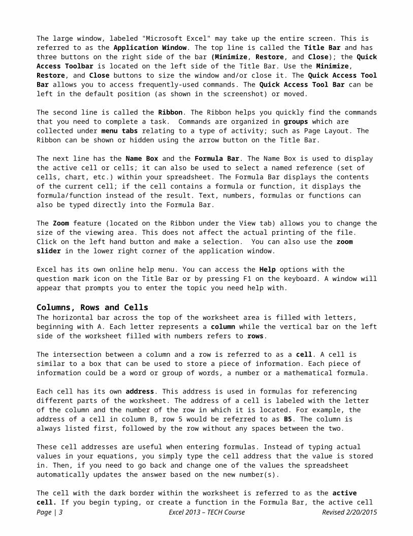
The large window, labeled "Microsoft Excel" may take up the entire screen. This is referred to as the Application Window. The top line is called the Title Bar and has three buttons on the right side of the bar (Minimize, Restore, and Close); the Quick Access Toolbar is located on the left side of the Title Bar. Use the Minimize, Restore, and Close buttons to size the window and/or close it. The Quick Access Tool Bar allows you to access frequently-used commands. The Quick Access Tool Bar can be left in the default position (as shown in the screenshot) or moved.

The second line is called the Ribbon. The Ribbon helps you quickly find the commands that you need to complete a task. Commands are organized in groups which are collected under menu tabs relating to a type of activity; such as Page Layout. The Ribbon can be shown or hidden using the arrow button on the Title Bar.

The next line has the Name Box and the Formula Bar. The Name Box is used to display the active cell or cells; it can also be used to select a named reference (set of cells, chart, etc.) within your spreadsheet. The Formula Bar displays the contents of the current cell; if the cell contains a formula or function, it displays the formula/function instead of the result. Text, numbers, formulas or functions can also be typed directly into the Formula Bar.

The Zoom feature (located on the Ribbon under the View tab) allows you to change the size of the viewing area. This does not affect the actual printing of the file. Click on the left hand button and make a selection. You can also use the zoom slider in the lower right corner of the application window.

Excel has its own online help menu. You can access the Help options with the question mark icon on the Title Bar or by pressing F1 on the keyboard. A window will appear that prompts you to enter the topic you need help with.

Columns, Rows and CellsThe horizontal bar across the top of the worksheet area is filled with letters, beginning with A. Each letter represents a column while the vertical bar on the left side of the worksheet filled with numbers refers to rows.

The intersection between a column and a row is referred to as a cell. A cell is similar to a box that can be used to store a piece of information. Each piece of information could be a word or group of words, a number or a mathematical formula.

Each cell has its own address. This address is used in formulas for referencing different parts of the worksheet. The address of a cell is labeled with the letter of the column and the number of the row in which it is located. For example, the address of a cell in column B, row 5 would be referred to as B5. The column is always listed first, followed by the row without any spaces between the two.

These cell addresses are useful when entering formulas. Instead of typing actual values in your equations, you simply type the cell address that the value is stored in. Then, if you need to go back and change one of the values the spreadsheet automatically updates the answer based on the new number(s).

The cell with the dark border within the worksheet is referred to as the active cell. If you begin typing, or create a function in the Formula Bar, the active cell will be populated. Each cell may contain text, numbers, or dates. You can enter up to 32,000 characters in each cell (equivalent to a 44 page report!).

Worksheets and WorkbooksA worksheet is made up of up to 17,179,869,180 individual cells. The first 26 columns are lettered A through Z. Excel then begins lettering the 27th column with AA and so on. In a single Excel worksheet there are 16,384 columns (lettered A-XFD) and 1,048,576 rows (numbered 1-1,048,576), however, the more data you have in a worksheet, the less manageable it becomes!

Toward the bottom of the Excel window is a small tab that identifies each sheet in the workbook (file). If there are multiple sheets, you can use the tabs to easily identify what data is stored on each sheet. When you begin a new workbook, the tabs default to being labeled Sheet1, Sheet2, etc. Worksheets can be renamed, moved, copied and deleted by right-clicking on a sheet and selecting the desired command.

Moving Around in ExcelWhen Excel starts, a new worksheet opens. What is currently visible is only a small portion of what is available for you to use. In order to move to areas that you cannot see, you can:

Use the scroll bars Use the keys described in the table below


Keystroke ResultTab Move one cell to the rightShift + Tab Move one cell to the leftArrow key Move one cell in the direction of the arrowCtrl + arrow key Move in the direction of the arrow to the last cell before a blank cell, or to the edge of

the worksheet if all cells are blankPage Up Moves up one screenPage Down Moves down one screenHome Moves to the beginning of the rowCtrl + Home Moves to cell A1Ctrl + End Moves to the last cell containing data (in the bottom right of the worksheet)

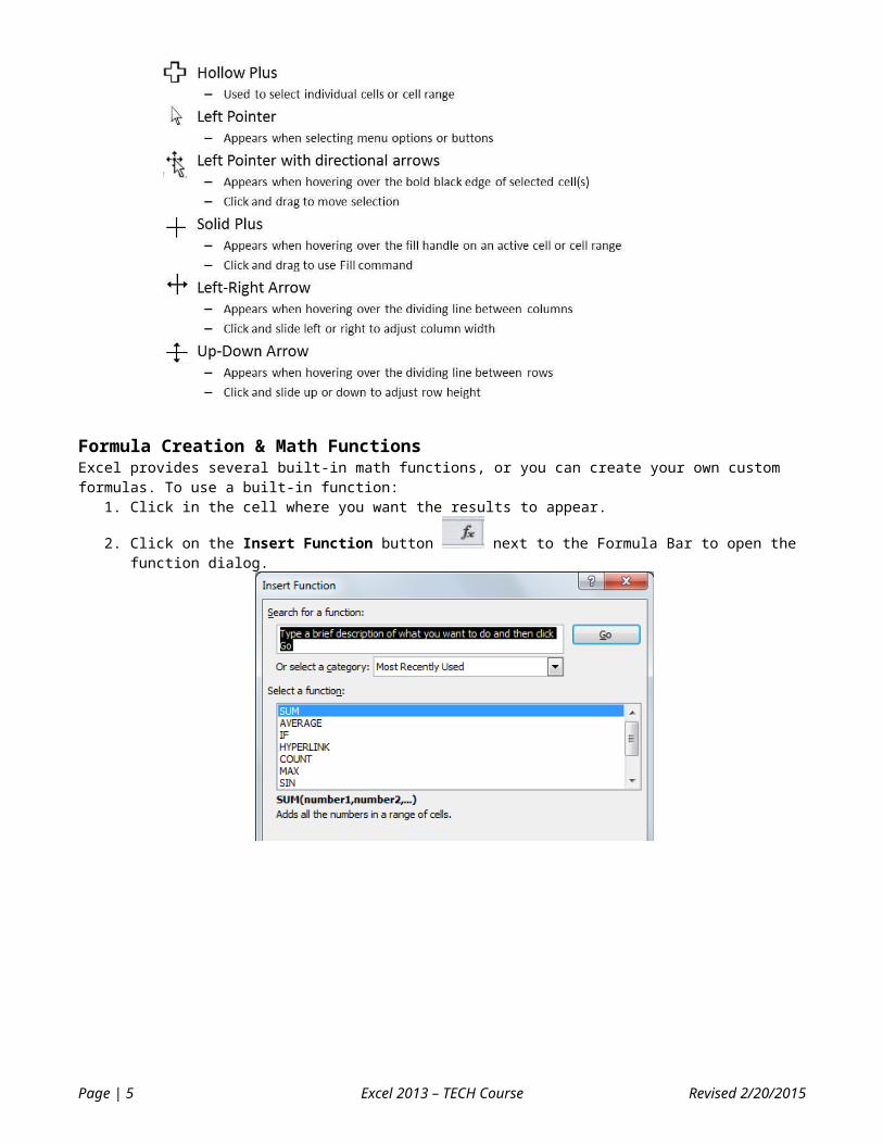
Excel Cursors & PointersExcel uses several unique cursors and pointers that are used for different functions. The table below depicts each pointer and its application.

Formula Creation & Math FunctionsExcel provides several built-in math functions, or you can create your own custom formulas. To use a built-in function:

1. Click in the cell where you want the results to appear.

2. Click on the Insert Function button next to the Formula Bar to open the function dialog.


3. From within the Insert Function dialog box, you can search for a function by name or select a category in the Function category list. All of the associated functions are listed below the function category, with a description of the function and its arguments below. Note: the Insert Function dialog box automatically displays most recently used functions for the function category.

4. After selecting the function you want, click OK to close the dialog box (Note: some functions have variations available with different arguments and results; a description of each function is listed at the bottom of the dialog box when you select it; always be sure you are using the correct function.)

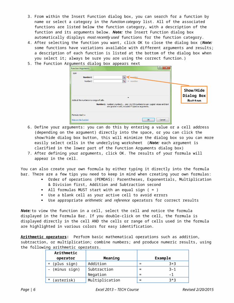
5. The Function Arguments dialog box appears next

6. Define your arguments: you can do this by entering a value or a cell address (depending on the argument) directly into the space, or you can click the show/hide dialog box button, this will minimize the dialog box so you can more easily select cells in the underlying worksheet (Note: each argument is clarified in the lower part of the Function Arguments dialog box)

7. After defining your arguments, click OK. The results of your formula will appear in the cell.

You can also create your own formula by either typing it directly into the formula bar. There are a few tips you need to keep in mind when creating your own formulas:

Order of operations (PEMDAS): Parentheses, Exponentials, Multiplication & Division first, Addition and Subtraction second

All formulas MUST start with an equal sign ( = ) Use a blank cell as your active cell to avoid errors Use appropriate arithmetic and reference operators for correct results

Note: to view the function in a cell, select the cell and notice the formula displayed in the Formula Bar. If you double-click on the cell, the formula is displayed directly in the cell AND the cells or range of cells used in the formula are highlighted in various colors for easy identification.

Arithmetic operators: Perform basic mathematical operations such as addition, subtraction, or multiplication; combine numbers; and produce numeric results, using the following arithmetic operators.

Arithmeticoperator Meaning Example

+ (plus sign) Addition = 3+3– (minus sign) Subtraction

Negation= 3–1= –1

* (asterisk) Multiplication = 3*3/ (forward slash) Division = 3/3% (percent sign) Percent = 20%^ (caret) Exponent = 3^2

Reference operators: Combine ranges of cells for calculations with the following operators.Referenceoperator Meaning Example: (colon) Range operator, which produces one reference to all

the cells between two references, including the two references

B5:B15

, (comma) Union operator, which combines multiple references into one reference

SUM(B5:B15,D5:D15)


Show/Hide Dialog Box

Button

Sorting and Filtering DataSortingOne of the more useful features of Excel is the ability for it to sort and filter a data set with ease. A dataset can be sorted by one or more columns, in ascending or descending order. Care must be taken when sorting data that the integrity of the dataset is retained; for instance, if you select one column of data that you want sorted, then data in adjoining cells may not always get sorted with the data selected. (Typically, however, Excel will warn you if there is data adjacent to the selected data and ask if you want to sort only the data selected or all of the data).

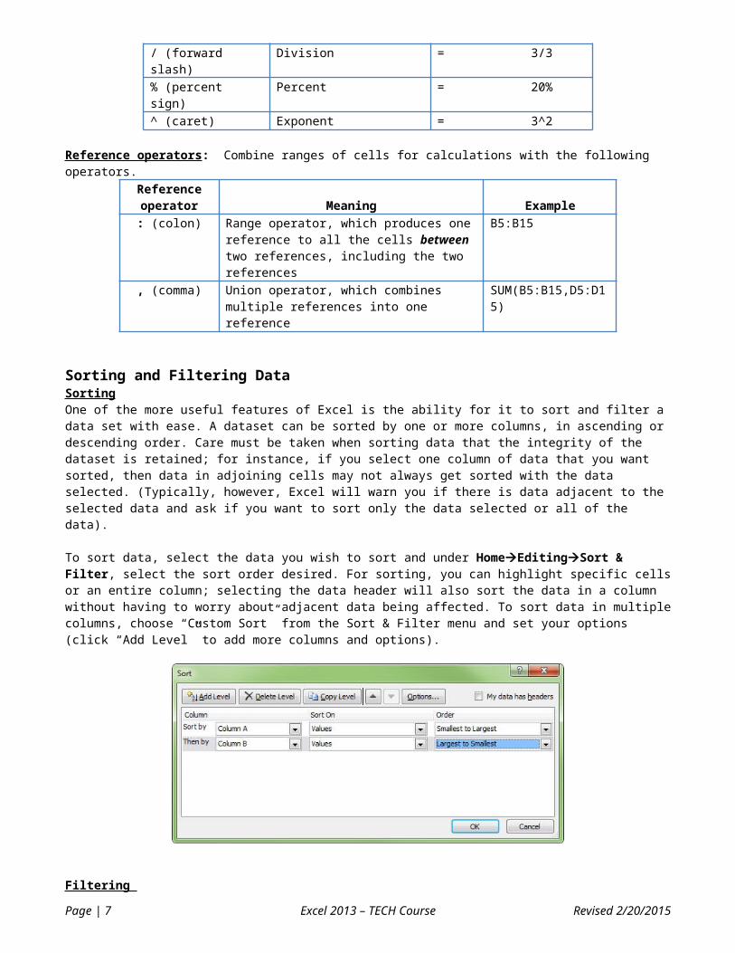
To sort data, select the data you wish to sort and under HomeEditingSort & Filter, select the sort order desired. For sorting, you can highlight specific cells or an entire column; selecting the data header will also sort the data in a column without having to worry about adjacent data being affected. To sort data in multiple columns, choose “Custom Sort” from the Sort & Filter menu and set your options (click “Add Level” to add more columns and options).

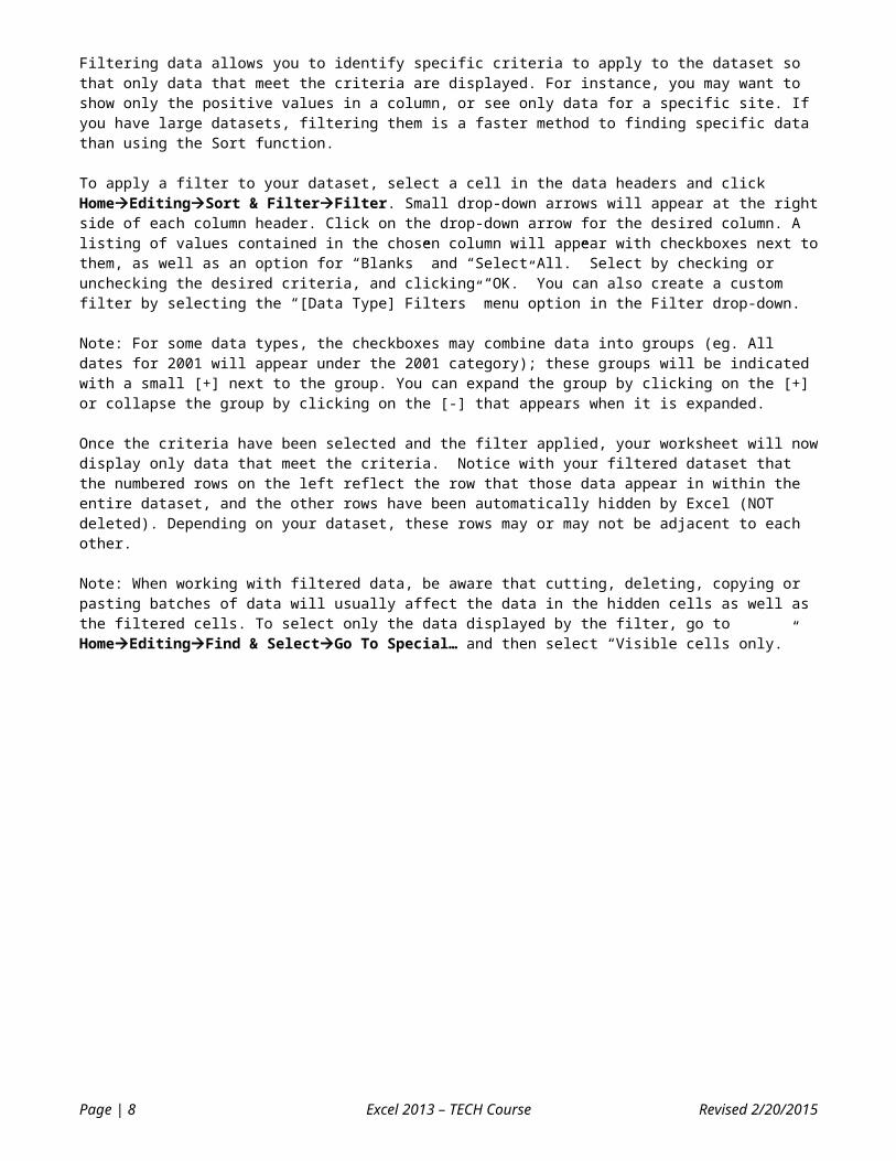
Filtering Filtering data allows you to identify specific criteria to apply to the dataset so that only data that meet the criteria are displayed. For instance, you may want to show only the positive values in a column, or see only data for a specific site. If you have large datasets, filtering them is a faster method to finding specific data than using the Sort function.

To apply a filter to your dataset, select a cell in the data headers and click HomeEditingSort & FilterFilter. Small drop-down arrows will appear at the right side of each column header. Click on the drop-down arrow for the desired column. A listing of values contained in the chosen column will appear with checkboxes next to them, as well as an option for “Blanks” and “Select All.” Select by checking or unchecking the desired criteria, and clicking “OK.” You can also create a custom filter by selecting the “[Data Type] Filters” menu option in the Filter drop-down.

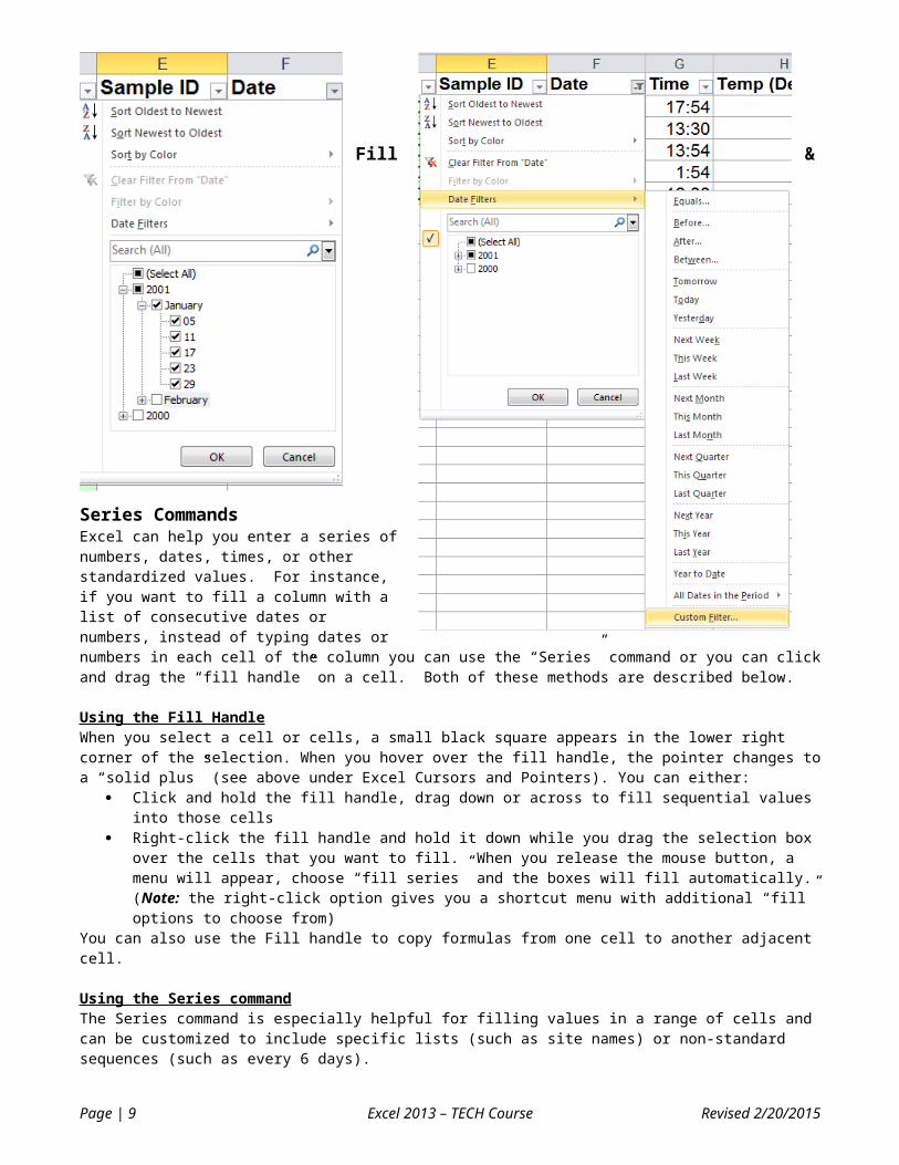
Note: For some data types, the checkboxes may combine data into groups (eg. All dates for 2001 will appear under the 2001 category); these groups will be indicated with a small [+] next to the group. You can expand the group by clicking on the [+] or collapse the group by clicking on the [-] that appears when it is expanded.

Once the criteria have been selected and the filter applied, your worksheet will now display only data that meet the criteria. Notice with your filtered dataset that the numbered rows on the left reflect the row that those data appear in within the entire dataset, and the other rows have been automatically hidden by Excel (NOT deleted). Depending on your dataset, these rows may or may not be adjacent to each other.

Note: When working with filtered data, be aware that cutting, deleting, copying or pasting batches of data will usually affect the data in the hidden cells as well as the filtered cells. To select only the data displayed by the filter, go to HomeEditingFind & SelectGo To Special… and then select “Visible cells only.”


Fill & Series CommandsExcel can help you enter a series of numbers, dates, times, or other standardized values. For instance, if you want to fill a column with a list of consecutive dates or numbers, instead of typing dates or numbers in each cell of the column you can use the “Series” command or you can click and drag the “fill handle” on a cell. Both of these methods are described below.

Using the Fill HandleWhen you select a cell or cells, a small black square appears in the lower right corner of the selection. When you hover over the fill handle, the pointer changes to a “solid plus” (see above under Excel Cursors and Pointers). You can either:

Click and hold the fill handle, drag down or across to fill sequential values into those cells Right-click the fill handle and hold it down while you drag the selection box over the cells that you want to fill.

When you release the mouse button, a menu will appear, choose “fill series” and the boxes will fill automatically. (Note: the right-click option gives you a shortcut menu with additional “fill” options to choose from)

You can also use the Fill handle to copy formulas from one cell to another adjacent cell.

Using the Series commandThe Series command is especially helpful for filling values in a range of cells and can be customized to include specific lists (such as site names) or non-standard sequences (such as every 6 days).

To use the Series command: Select the cell that contains the first value. Using your mouse, click and drag the hollow plus pointer so the cells that you wish to fill are highlighted. Under HomeEditingFill choose Series. The Series dialog box will appear. Select the appropriate options for your series


Creating Custom SeriesCustom series are useful for text (such as site names or months of the year, etc.) or mixed text/numeric values that are always in the same order (ie: FY12, FY13, etc.). There are two ways to create a custom series:

Enter first two values of series (ie. Year 1, Year 2) Select both cells and drag fill handle to fill desired cells

OR: First, define a custom list: FileExcel OptionsAdvancedGeneralEdit Custom Lists Select cells to be filled, with starting value in first cell then select HomeFillSeries and select AutoFill under the

Type option. Alternately, you can select the starting cell and drag fill handle to fill desired cells

Creating chartsCharts can emphasize important points in your data and make them easier to understand. Using charts, you are able to get your point across efficiently and quickly, embedding them in reports or presenting them to interested audiences.

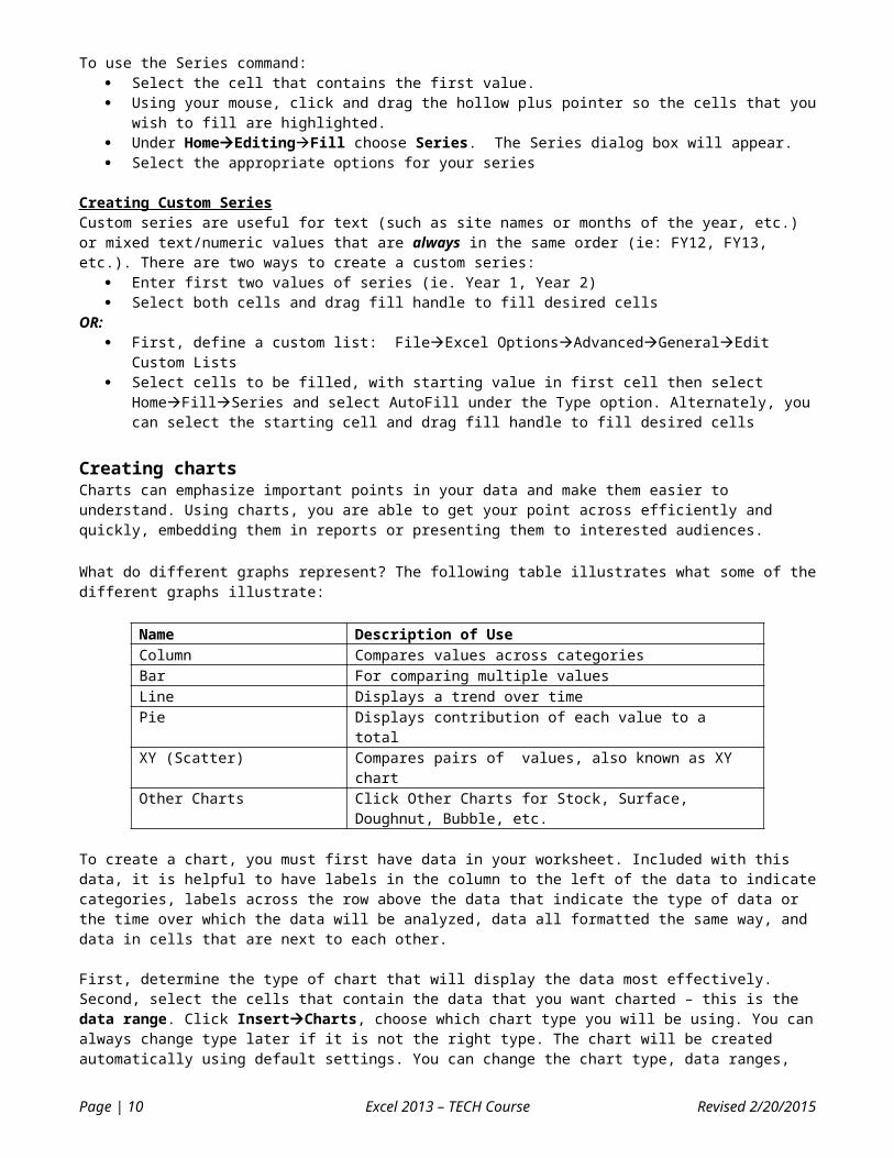
What do different graphs represent? The following table illustrates what some of the different graphs illustrate:

Name Description of UseColumn Compares values across categoriesBar For comparing multiple valuesLine Displays a trend over timePie Displays contribution of each value to a totalXY (Scatter) Compares pairs of values, also known as XY chartOther Charts Click Other Charts for Stock, Surface, Doughnut, Bubble, etc.

To create a chart, you must first have data in your worksheet. Included with this data, it is helpful to have labels in the column to the left of the data to indicate categories, labels across the row above the data that indicate the type of data or the time over which the data will be analyzed, data all formatted the same way, and data in cells that are next to each other.

First, determine the type of chart that will display the data most effectively. Second, select the cells that contain the data that you want charted – this is the data range. Click InsertCharts, choose which chart type you will be using. You can always change type later if it is not the right type. The chart will be created automatically using default settings. You can change the chart type, data ranges, plotting methods, titles, legend placement, and chart placement using various tools in the Chart Tools tab set that appears when the chart is selected. Importing TextSome types of air monitors supply data in a text format. These files are often identified by the .txt suffix (example: february00.txt). Text files contain lines of characters, including both numbers and letters. To divide these lines of text into columns of data, characters, including commas or tabs are inserted to separate each field or column of data (referred to as delimited text). Text data can also be in a fixed-width format, where the fields are aligned in columns with spaces between each field. Excel’s Text Import tool can import both of these text file data formats. The Text Importing function takes the lines of characters and converts them into data contained within the columns and rows of an Excel file.

Choose Data Get External Data From Text. The import text dialog box appears. Choose the text file that you would like to import from Excel and double-click on it or single-click the file name, then click the Import button. Follow the instructions given by the Text Importing dialog boxes that follow.

PrintingPrint Preview & Layout OptionsBefore you print a worksheet it is recommended to preview the document first, click FilePrint (a preview image will appear before actually printing) to see how the sheet will look when you print it. The way pages appear in the preview window depends on the available fonts, the resolution of the printer, etc. and can be adjusted with some of the options available in the Print window (ie. Margins, Orientation, Paper size, Scaling).

To fit all the contents of your worksheet onto one page (or all columns or all rows on one page, etc.) you can adjust the Scaling options, however the size of the text/images will be shrunken to meet the specified scale.

You may notice that Excel wants to print more rows or columns than you want to. You can set the print area using Page LayoutSet Print Area (you must first select the range of cells to include in the print area).


Printing TitlesExcel can print headings or information in specified rows or columns on each page; this is useful when you have to print a file with multiple pages of information and need to refer to column/row headings on each page. Page LayoutPrint Titles opens the Page Setup dialog box. Enter the cell range for the Rows to repeat at top or Columns to repeat at left as desired (ie. A1:K1); if you don’t know the cell addresses, you can select the data directly by using the Show/Hide Dialog Box buttons.

If you want the Column or Row names (A, B, C and 1, 2, 3) to be displayed when printed, check the Row & Column Headings box.

Part 2: Activities Using ExcelThe following activities use skills and concepts discussed in Part 1. Reference the above information for additional guidance on the steps outlined below.

Activity 1: Basic Formula Creation1. Open the “O3Data.xls” file in the “TECH Computer Exercises” folder on your desktop.2. Review the data displayed in Sheet1; notice it is hourly ozone data for two monitoring sites for a 24-hour period.3. In a blank cell under the hourly average values for each site, create the following functions (remember to label your

functions with their name in an adjacent cell):a. COUNT number of data points in each data setb. 24-hour AVERAGE ppbv valuec. Minimum (MIN) value for 24 hoursd. Maximum (MAX) value for 24 hourse. Standard Deviation (STDEV) of daily readings

4. In cell G5, create a formula for Relative Percent Difference (RPD), comparing values for one hour only between Site1 & Site2

a. RPD formula: (“=((B5-E5)/AVERAGE(B5+E5))*100)”)b. When completed, grab the fill handle for cell G5 and drag-fill down to cell G28 to copy the RPD formula

for each remaining hour


Show/Hide Dialog Box

Button

Activity 2: Creating a Chart1. Open the “TEOMData.xls” file in the “TECH Computer Exercises” folder on your desktop.2. Review the data displayed in Sheet1; notice it is hourly PM data and associated MET data from a TEOM

Continuous PM sampler for a 24-hour period; the data at the bottom of the sheet has been extracted from the top dataset to make it easier for charting.

3. Select the bottom dataset, including headers, then InsertCharts and select Column.4. Your chart will be created within Sheet1; to make it easier to read and work with, right-click on the chart area and

select Move Chart. Move the chart to a new sheet. 5. Notice the dates on the horizontal chart axis are overlapping and are not needed for the chart. Remove the data:

a. Chart ToolsSelect Datab. Under Horizontal Axis Labels, click “Edit”

c. For the axis label range, click the button select only the data in the Time column; click OK.6. Add a Chart Title: Chart ToolsLayout, then click in the text box to type your own name7. Feel free to modify other elements of the chart layout, formatting, etc. using the Chart Tools available.

Activity 3: Display Data Using a Secondary Axis 1. Select the TEOM PM10 data series by clicking once on the series bar1. Right-click on the series and select Format Data Series; select Plot Series On Secondary Axis2. Notice how the series displays differently using two axes.3. To make the PM data series more distinct from the wind speed and air temp values, right-click on the PM series

again, select “Change Series Chart Type” and select Line4. For clarity, be sure to add titles to both axes by selecting Chart ToolsLayoutAxis Titles

a. Primary Vertical Axis Title: PM10 Concentration (ug/m3)b. Secondary Vertical Axis Title: Wind Speed (m/s) & Air Temperature (deg C)

Activity 4: Add a Trendline 1. Right-click on the PM10 line and select “Add Trendline”2. In the Format Trendline dialog box, select “linear” and also check the boxes to display equation and r-squared value

Activity 4: Importing Text Files1. Open a new blank workbook2. Select DataGet External DataFrom Text 3. Import data from the COData.txt text file in the desktop folder “TECH Computer Exercises”4. Use the Text Import Wizard Dialog Boxes:

a. Dataset is delimited b. Start import at Row1 so it captures the metadata, but scroll down the dataset and see that you could start at

Row33 to import data values only without the metadata; in this case there is also extraneous information at the end of the dataset that you can ignore.

c. Select TAB as the delimiter type and briefly scroll through the data preview to ensure the correct delimiter has been selected (note: you can try selecting a different delimiter type to see how it changes the way the data would be imported, but be sure to change it back to TAB before importing).

d. The final screen of the Wizard allows you to set various formats for the data being imported. In this case, there are no changes to be made. Click Finish.

e. Tell Excel where to paste the data upon import. Click OK.5. Once imported, review the data—does it look OK? What is notable about the data file?


Part 3: More Activities Using ExcelThe following activities are provided for students who have extra time and wish to practice with additional activities.

Activity 1: Converting Temperatures from Fahrenheit to Celsius1. From the TECH Computer Exercises folder on the desktop, open the Excel file called “PMMockData”2. Create a new column for Temp (degF) values (note the data already has a column for degC)3. Enter the formula in the first cell of the Celsius column to convert from degF to degC

Hint: degC = (degF-32) x (5/9)4. Use the Fill/Series command to fill the formula to the end of the degF values.

Activity 2: Mean, Standard Deviation, Max, Min, Charts1. From the TECH Computer Exercises folder on the desktop, open the Excel file called “PMMockData”2. Answer the following questions by creating formulas for the data set.

a) What is the average (mean) PM2.5 value for the data set?b) What is the standard deviation for the PM2.5 data set?c) What is the maximum PM2.5 value? On what date did it occur? d) What is the minimum PM2.5 value? On what date did it occur?

3. Create a chart showing the sampling date (x-axis) and PM2.5 value (y-axis). [InsertChartsLine] Label the X and Y axes and give a title to the graph.

4. When you have finished making the chart, add a trendline line and have the equation and r-squared value displayed on the graph.

Activity 3: PM2.5 concentrationPM2.5 filters were weighed before and after sampling and the atmospheric conditions were recorded. What were the PM2.5

concentrations in µg/m3? Set up an Excel spreadsheet to do the calculations.

filter wt before sampling (mg)

filter wt after sampling (mg)

Sampling period (hrs)

flow rate (L/min)

air pressure (mm Hg)

air temp (°C)

143.400 143.900 24 16.600 744 24150.300 150.900 24 16.800 743 20145.700 147.300 24 16.600 756 21

Activity 4: NOx Boiler EmissionsSuppose you want to calculate the emissions of NOx from the combustion of fuel in a boiler. This facility emits NOx at the rate of 3.92 lb/hr, and it is in operation for 8 hours/day, 5 days/week, 52 weeks/year. What are the emissions in tons per year (TPY)? What would the emissions of NOx be if this facility emitted combustion products continually for a year?

Activity 5: Calculating Vehicle Miles Traveled (VMT)1. From the TECH Computer Exercises folder on the desktop, open the Excel file called “OnroadExercise”2. Create formulas to calculate Yearly Vehicle Miles Traveled for all three categories of vehicles for each road. 3. Create formulas to calculate the Total VMT for paved, unpaved, and all roads.

a) What is the total VMT for Light Cars on all roads?b) What is the total VMT for Heavy Gas Vehicle for all roads?c) What is the total VMT for Heavy Diesel Vehicle for all roads?

4. Enter the calculated Total VMT figures for each vehicle category (all roads) into the Emissions Calculations portion of the worksheet.

5. Using the Emission Factors provided, calculate the Emissions in grams/year, pounds/year, and tons/year for each pollutant (NOTE: EFs are in grams/mile; REMINDER: Emissions=EF x VMT)a) What category of vehicle produced the highest VOC emissions?b) What category of vehicle produced the highest NOX emissions?c) What category of vehicle produced the lowest CO emissions?


units conversion software - northern arizona...

Documents