united states environmental protection … · environmental & occupational health ... lake...

UNITED STATES ENVIRONMENTAL PROTECTION AGENCY WASHINGTON D.C. 20460

OFFICE OF THE ADMINISTRATOR

SCIENCE ADVISORY BOARD

April 30, 2018

EPA-CASAC-18-001

The Honorable E. Scott Pruitt

Administrator

U.S. Environmental Protection Agency

1200 Pennsylvania Avenue, N.W.

Washington, D.C. 20460

Subject: CASAC Review of the EPA’s Risk and Exposure Assessment for the Review of the

Primary National Ambient Air Quality Standard for Sulfur Oxides (External Review Draft

- August 2017)

Dear Administrator Pruitt:

The Clean Air Scientific Advisory Committee (CASAC) Sulfur Oxides Panel met on September 18-19,

2017, and April 20, 2018, to peer review the EPA’s Risk and Exposure Assessment for the Review of the

Primary National Ambient Air Quality Standard for Sulfur Oxides (External Review Draft - August

2017), hereafter referred to as the Draft REA. The Chartered CASAC approved the report on April 20,

2018. The CASAC’s consensus responses to the agency’s charge questions and the individual review

comments from members of the CASAC Sulfur Oxides Panel are enclosed.

There are several recommendations for strengthening and improving the document highlighted below

and detailed in the consensus responses. The CASAC believes that, with these recommended changes,

the document will serve its intended purpose of presenting scientifically-sound quantitative assessments

of risks and exposures for the agency’s review of the Sulfur Oxides Primary (Health-based) National

Ambient Air Quality Standards (NAAQS).

The CASAC finds the introductory and background material presented in Chapter 1 of the Draft REA to

be adequately communicated and appropriately characterized. The EPA should consider adding an

Executive Summary, to provide a succinct summary of the primary purpose, overall approach, and

major outcomes. The CASAC finds the conceptual model summarized in Chapter 2 to be very useful. A

brief but clear explanation for why air quality conditions were simulated to only just meet the current

standard should be added. The Draft REA would be enhanced by hyperlinks to HERONET and other

web-accessible references.

The discussion of ambient air concentrations in Chapter 3 is generally well written. The CASAC

recommends documentation of the rationale for why the three study areas were selected from the 100

candidate areas specified in the REA Planning Document. The rationale for not including integrated iron

and steel mill sources should also be provided. The CASAC finds that the EPA has not fully addressed

the possible importance of emissions from smelters and integrated iron and steel mills as modifiers of

the effect of sulfur dioxide (SO2) on asthma. AERMOD model performance should be evaluated by

comparing modeled and measured concentrations paired in time and space. Model biases should be

discussed and accounted for in the final REA. Model performance criteria should be discussed. The

rationale should be provided for adjusting the emissions from one primary source for each study area

without adjusting for other large sources. The nonlinear processes from emissions to ambient

concentrations should be documented. In addition, the EPA is encouraged to start requiring states to

report all twelve of the 5-minute SO2 measurements within each hour in order to establish an adequate

database for future SO2 NAAQS reviews. The short-duration measurements allow for the examination of

consecutive elevated 5-minute SO2 concentrations to evaluate durations of plume touchdowns and

downward mixing. This can provide a better understanding of exposure durations and patterns,

especially when SO2 concentrations exceed the 200 ppb health benchmark.

The CASAC finds that the presentation of key aspects of the exposure modeling in Chapter 4 are

generally sound and the detailed analysis is thorough, although clarification is needed in some places.

The CASAC recommends that the EPA explicitly state how the populations in the modeled areas are

representative of the U.S. population. The CASAC suggests that the EPA explicitly justify the decision

to select specific variables for simulation and modeling of the at-risk population. Further, the EPA

should refer specifically to race in relation to at-risk subpopulations. For future NAAQS reviews, the

CASAC suggests that the EPA develop a strategy to effectively collect and use information on race

when collecting activity data. It is important to consider how one would collect this information, and the

form of data needed, to effectively incorporate race into the analysis.

The derivation of the exposure-response function is sound and follows that of previous NAAQS

reviews. The CASAC recommends that the EPA explicitly reference the previous SO2 NAAQS reviews

in which both probit and logit regression models were considered for the exposure-response relationship,

and in which the selection of the probit functional form was justified. In Figure 4-1, the prediction

interval around the mean appears to be mislabeled and is apparently a confidence interval. This should

be verified and if necessary, relabeled or clarified. If the labeled 5-95% prediction interval is actually a

confidence interval, then the analysis should be run again, with a comparison of the prediction interval

and confidence interval shown side by side in the figure.

The prevalence of asthma varies by race/ethnicity and is highest in African-Americans. Asthma

prevalence is also higher among obese individuals than in the general population. The CASAC therefore

recommends that race and obesity be included as characteristics of the population, and levels of SO2

exposure and risk of adverse effects associated with the current SO2 standard be assessed in these sub-

groups. The CASAC recognizes that detailed data for African-Americans and obese individuals may not

be available, limiting the ability to include them in the risk assessment and exposure models in the

manner that was used for other demographic variables. However, it is recommended that the agency use

whatever data are available and suitable to assess exposure and risk influence by race and obesity. If it is

not possible to include these variables in the analysis, then sensitivity analyses should be considered,

and, at a minimum, the possibility of heterogeneity in associations across population subgroups and

uncertainty should be considered as they relate to the margin of safety.

The characterization of uncertainty and representation of variability is appropriate and well organized.

The CASAC concurs that it is appropriate to use observed variability in the input data when these data

are available and sufficiently representative. In the case of the exposure-response curve (Figure 4-1), it

is unclear whether this was a confidence interval or a prediction interval. The CASAC recommends that

the high end of risk (i.e. 95% end of the prediction interval) rather than the confidence interval be used.

The CASAC has identified a few additional uncertainties that should be considered in the analysis.

These include uncertainties due to: AERMOD inputs, algorithms, and outputs; the study areas and their

spatial make-up; the spatial overlap of poverty and race (which will affect asthma prevalence rates) and

spatial distribution of the SO2 concentrations; extrapolations of key quantities from one geographic area

to another; and the contributions of microenvironmental variables.

The CASAC appreciates the opportunity to provide advice on the Draft REA and looks forward to the

agency’s response.

Sincerely,

/S/ /S/

Dr. Louis Anthony Cox Jr., Chair Dr. Ana Diez Roux, Immediate Past Chair

Clean Air Scientific Advisory Committee Clean Air Scientific Advisory Committee

Enclosures

i

NOTICE

This report has been written as part of the activities of the EPA's Clean Air Scientific Advisory

Committee (CASAC), a federal advisory committee independently chartered to provide extramural

scientific information and advice to the Administrator and other officials of the EPA. The CASAC

provides balanced, expert assessment of scientific matters related to issues and problems facing the

agency. This report has not been reviewed for approval by the agency and, hence, the contents of this

report do not represent the views and policies of the EPA, nor of other agencies within the Executive

Branch of the federal government. In addition, any mention of trade names or commercial products does

not constitute a recommendation for use. The CASAC reports are posted on the EPA website at:

http://www.epa.gov/casac.

http://www.epa.gov/casac

ii


Clean Air Scientific Advisory Committee

Sulfur Oxides Panel

CHAIR

Dr. Louis Anthony (Tony) Cox, Jr., President, Cox Associates, Denver, CO

IMMEDIATE PAST CHAIR

Dr. Ana V. Diez Roux, Dean, School of Public Health, Drexel University, Philadelphia, PA

CASAC MEMBERS

Dr. James Boylan, Program Manager, Planning & Support Program, Air Protection Branch, Georgia

Department of Natural Resources, Atlanta, GA

Dr. Judith Chow, Nazir and Mary Ansari Chair in Entrepreneurialism and Science and Research

Professor, Division of Atmospheric Sciences, Desert Research Institute, Reno, NV

Dr. Jack Harkema, Distinguished University Professor, Department of Pathobiology and Diagnostic

Investigation, College of Veterinary Medicine, Michigan State University, East Lansing, MI

Dr. Elizabeth A. (Lianne) Sheppard, Professor of Biostatistics and Professor and Assistant Chair of

Environmental & Occupational Health Sciences, School of Public Health, University of Washington,

Seattle, WA

CONSULTANTS

*Mr. George A. Allen, Senior Scientist, Northeast States for Coordinated Air Use Management

(NESCAUM), Boston, MA

Dr. John R. Balmes, Professor, Department of Medicine, Division of Occupational and Environmental

Medicine, University of California, San Francisco, San Francisco, CA

Dr. Aaron Cohen, Consulting Scientist, Health Effects Institute, Boston, MA

Dr. Alison C. Cullen, Professor, Daniel J. Evans School of Public Policy and Governance, University

of Washington, Seattle, WA

Dr. Delbert Eatough, Professor of Chemistry, Department of Chemistry and Biochemistry , Brigham

Young University, Provo, UT

*Recused from review

iii

Dr. H. Christopher Frey, Glenn E. Futrell Distinguished University Professor, Department of Civil,

Construction and Environmental Engineering, College of Engineering, North Carolina State University,

Raleigh, NC

Dr. William C. Griffith, Associate Director, Department of Environmental and Occupational Health

Sciences, Institute for Risk Analysis & Risk Communication, School of Public Health, University of

Washington, Seattle, WA

Dr. Steven Hanna, President, Hanna Consultants, Kennebunkport, ME

Dr. Daniel Jacob, Professor, Atmospheric Sciences, School of Engineering and Applied Sciences,

Harvard University, Cambridge, MA

Dr. Farla Kaufman, Epidemiologist, Office of Environmental Health Hazard Assessment,

Reproductive and Cancer Hazards Assessment Section, California EPA, Sacramento, CA

Dr. Donna Kenski, Data Analysis Director, Lake Michigan Air Directors Consortium, Rosemont, IL

Dr. David Peden, Distinguished Professor of Pediatrics, Medicine & Microbiology/Immunology,

School of Medicine, University of North Carolina at Chapel Hill, Chapel Hill, NC, United States

Dr. Richard Schlesinger, Associate Dean, Dyson College of Arts and Sciences, Pace University, New

York, NY

Dr. Frank Speizer, Edward Kass Distinguished Professor of Medicine, Channing Division of Network

Medicine, Brigham and Women's Hospital and Harvard Medical School, Boston, MA

Dr. James Ultman, Professor, Chemical Engineering, Bioengineering Program, Pennsylvania State

University, University Park, PA

Dr. Ronald Wyzga, Technical Executive, Air Quality Health and Risk, Electric Power Research

Institute, Palo Alto, CA

SCIENCE ADVISORY BOARD STAFF

Mr. Aaron Yeow, Designated Federal Officer, U.S. Environmental Protection Agency, Science

Advisory Board, Washington, DC

iv


Clean Air Scientific Advisory Committee

CHAIR

Dr. Louis Anthony (Tony) Cox, Jr., President, Cox Associates, Denver, CO

MEMBERS

Dr. James Boylan, Program Manager, Planning & Support Program, Air Protection Branch, Georgia

Department of Natural Resources, Atlanta, GA

Dr. Judith Chow, Nazir and Mary Ansari Chair in Entrepreneurialism and Science and Research

Professor, Division of Atmospheric Sciences, Desert Research Institute, Reno, NV

Dr. Ivan J. Fernandez, Distinguished Maine Professor, School of Forest Resources and Climate

Change Institute, University of Maine, Orono, ME

Dr. Jack Harkema, Distinguished University Professor, Department of Pathobiology and Diagnostic

Investigation, College of Veterinary Medicine, Michigan State University, East Lansing, MI

Dr. Elizabeth A. (Lianne) Sheppard, Professor of Biostatistics and Professor and Assistant Chair of

Environmental & Occupational Health Sciences, School of Public Health, University of Washington,

Seattle, WA

*Dr. Larry Wolk, Executive Director & Chief Medical Officer, Colorado Department of Public Health

& Environment, Denver, CO

*Recused from review

SCIENCE ADVISORY BOARD STAFF

Mr. Aaron Yeow, Designated Federal Officer, U.S. Environmental Protection Agency, Science

Advisory Board, Washington, DC

1

Consensus Responses to Charge Questions on the EPA’s

Risk and Exposure Assessment for the Review of the Primary National Ambient Air Quality Standard

for Sulfur Oxides (External Review Draft - August 2017)

Introduction and Background for the Risk and Exposure Assessment (Chapter 1)

1. Does the Panel find the introductory and background material, including that pertaining to previous

SO2 exposure/risk assessments, to be clearly communicated and appropriately characterized?

The CASAC finds the introductory and background material presented in Chapter 1 of the Draft REA,

including that pertaining to the previous SO2 exposure/risk assessments, to be adequately communicated

and appropriately characterized. The introductory chapter is clearly and concisely written.

The EPA should consider adding an Executive Summary, to provide a succinct summary of the primary

purpose, overall approach, and major outcomes.

Conceptual Model and Overview of Assessment Approach (Chapter 2)

2. Does the Panel find the conceptual model summarized in Section 2.1 to adequately and appropriately

summarize the key aspects of the conceptual model for the assessment?

The CASAC finds the conceptual model summarized in Chapter 2 (Section 2.1) to be very useful. Figure

2-1 illustrates the conceptual model well, but should be redrafted to be more readable.

3. Does the overview in Section 2.2 clearly communicate key aspects of the approach implemented for

this assessment?

The overview in Section 2.2 clearly communicates the key aspects of the approach used for this

assessment. A brief, but clear explanation for why “air quality conditions simulated to just meet the

current standard” (p. 2-6, lines 28-29) were used should be added.

Both Chapters 1 and 2, as well as the rest of the document, would be enhanced with hotlinks to

HERONET and other web-accessible references.

Ambient Air Concentrations (Chapter 3)

Overall, Chapter 3 is well written and includes study area characteristics, air quality modeling inputs, a

description of the rationale used to select air quality model receptors for exposure modeling, adjustments

to design values, and estimation of continuous 5-minute data.

4. Does the Panel find the description of the three study areas and their key aspects (Section 3.3) to be

clear and technically appropriate?

2

The five criteria used to select the three study areas are sound, as they include large geographical

regions, diverse SO2 emission sources, sufficient air quality monitoring and modeling data, a design

value near the current SO2 standard (75 ppm), and populations greater than 100,000. However, the three

study areas (i.e., Fall River, MA; Tulsa, OK; and Indianapolis, IN) differ from the nine candidate areas

identified in the Risk and Exposure Assessment (REA) Planning Document (U.S. EPA 2017a). The

CASAC recommends that the EPA document the rationale for selecting the three study areas from the

100 candidate areas and why certain candidate areas from the REA Planning Document were excluded

from the Draft REA (i.e., Detroit, MI and Savannah, GA).

The Draft REA does not include areas with integrated iron and steel mills, important SO2 sources for

assessing population exposure. As noted in the June 30, 2017, CASAC review of the Second Draft ISA

(EPA-CASAC-17-003): “It is also important to highlight the contributions of emissions from smelters

and integrated iron and steel mills as these may explain some high values in the data shown.” The

agency response on August 16, 2017, states that smelters and other metal processing facilities would be

addressed in the final version of the ISA. As these sources are particularly important with respect to the

Draft REA, the CASAC recommends that the EPA explain the reasons that integrated iron and steel mill

sources are not included in the Draft REA. The CASAC finds that the EPA has not fully addressed the

possible importance of emission from smelters and integrated iron and steel mills as modifiers of the

effect of SO2 on asthma. This is evident in the REA because this perspective was not taken into account

in the selection of study areas. The CASAC recommends EPA strengthen its attention to this matter in

the REA and is concerned that it was not adequately addressed in the ISA. Further details can be found

in Dr. Delbert Eatough’s individual comments.

One of the candidate areas from the REA Planning Document (Detroit, MI) contains a variety of

emission sources, along with six SO2 monitoring sites that meet the Draft REA selection criteria.

Although it may be too late at this stage of the process to include a fourth study area, an exercise

demonstrating that the addition of Detroit as a new study area will not alter the outcome of overall

exposure assessment should be provided. (Further details can be found in Dr. Delbert Eatough’s

individual comments.)

In the Draft REA, the AERMOD modeling uses the 2011 National Emissions Inventory (NEI) and 2011-

2013 ambient SO2 data. This is not consistent with the Second Draft ISA (U.S. EPA 2016) and the Draft

Policy Assessment (U.S. EPA 2017b), which use the 2014 NEI and 2013-2015 ambient SO2 data. This

inconsistency and the impact of the inconsistency needs to be addressed (due to changes in emission

estimates from 2011 to 2014 and the uncertainties associated with using ambient SO2 measurements

from different years for AERMOD and exposure modeling.)

The CASAC recommends the addition of a map for each of the three study areas to specify the

locations, types, and magnitudes of SO2 emission sources; upper-air and surface meteorological stations;

SO2 monitors (indicating whether or not sequential or hourly maximum 5-minute concentrations are

available); and the dimensions of each model-based study area.

5. Does the Panel find the description of the air quality modeling done to estimate the spatial variation

in 1-hour concentrations (Section 3.2) to be technically sound and clearly communicated?

Section 3.2 documents model inputs (e.g., meteorological measurements, surface characteristics and

land use, emission sources, terrain, and air quality receptor locations). The designation of ambient

3

monitors as background sites for each study area needs to be clarified. The representativeness of

meteorological data used to determine the number of hours to be excluded from the calculation of

background concentrations needs to be justified. As Indianapolis has the most complex set of point

sources, the approaches taken to estimate hourly background concentrations stratified by season need to

be documented.

The fact that the background concentrations are added to the estimated source concentrations should be

stated explicitly. As the EPA relied on input data developed by the states to build their analyses for the

Draft REA, the states’ contributions should be acknowledged.

The representativeness of upper-air and surface meteorological data needs further documentation.

Depending on atmospheric turbulence, larger fluctuations in 5-minute SO2 concentrations can occur

closer to the source. Therefore, the observed 5-minute variability at the monitor may underestimate the

variability (i.e., lower peak-to-mean ratios) actually observed at the location of the design concentration.

AERMOD model performance was evaluated using simple QQ-plots, not paired in time and space, to

compare model and measured concentrations. However, for dispersion modeling in support of health

studies, where the model must capture concentrations at specified time periods and locations, additional

measures of bias and data scatter are important. The CASAC recommends evaluating AERMOD model

performance by comparing modeled and measured concentrations paired in time and space. One way to

do this would be by generating Q-Q plots to compare measured 1-hour SO2 concentrations and modeled

1-hour SO2 concentrations by time-of-day, day-of-week (weekday/weekend), and season-of-year for all

SO2 monitors located in the study areas. (See Dr. James Boylan’s individual comments and model

performance evaluation in Appendix B for further details). Model biases should be discussed and

accounted for in the final REA. In addition, the REA needs to discuss “acceptable” model performance

criteria for the statistics presented in the tables. Model performance can also be evaluated using the

BOOT model evaluation software to determine model mean bias and scatter. When the BOOT software

was used to evaluate AERMOD performance using hourly data from Fall River, Indianapolis, and Tulsa,

the mean bias and scatter are about the same magnitude as the mean itself. This performance, which is

typical of AERMOD projections, does not satisfy published criteria for dispersion models applied to

rural or urban field studies. Trends in time of day (better performance for daytime), wind speed (better

performance for higher wind speeds), and site (worse performance for sites in Indianapolis) are

apparent. Such evaluations should be included in the REA’s discussion of uncertainty and variability.

Further details can be found in Dr. Steven Hanna’s individual comments.

6. To simulate air quality just meeting the current standard, we have adjusted model predicted 1-hour

SO2 concentrations using a proportional approach focusing on the primary emissions source in each

area to reduce the modeled concentrations at the highest air quality receptor to meet the current

standard (Section 3.4). Considering the goal of the analyses is to provide a characterization of air

quality conditions that just meet the current standard and considering the associated uncertainties, what

are the Panel’s views on this approach?

The approach taken to scale SO2 concentrations to design values needs further explanation. The

rationale for adjusting the emissions from one primary source for each study area, while not recognizing

the presence of other large sources, should be explained. The application of scaling methods implies that

the emissions increase or decrease accordingly, which may also affect the plume rise. Plume rise affects

4

downwind ground-level concentrations. The nonlinear processes from emissions to ambient

concentrations need to be documented.

7. A few approaches were used to extend the existing ambient air monitoring data to reflect temporal

patterns in the study area (Section 3.5). Does the Panel find the approaches used below to be technically

sound and clearly communicated?

a. Data substitution approach for missing 1-hour, 5-minute maximum, or 5-minute continuous ambient

air monitor concentrations (Section 3.5.1).

b. Estimating pattern of within-hour 5-minute continuous concentrations where 1-hour average and 5-

minute maximum are known (Section 3.5.2).

c. Combining pattern of continuous 5-minute concentrations within each hour from monitors in or near

the study area with the modeled 1-hour concentrations (Section 3.5.3).

The monitor from Wayne County (i.e., Detroit, MI) is used as a surrogate monitor for Indianapolis,

based on the geographic region and a similar design value. Comparisons should be made to demonstrate

the deviations of estimated 5-minute data and representativeness of meteorological conditions reported

by the surrogate monitor.

The representativeness of data from one SO2 monitoring site located several kilometers from the major

sources needs to be explained. For Tulsa, only one coal-burning electricity generating unit (EGU) is

used for modeling and model performance was compared with one monitoring site reporting twelve 5-

minute data. The reasons for not modeling source impacts from other major sources (e.g., Public Service

Company of Oklahoma Northeastern Plant and OG&E Muskogee Generating Station) should be

provided. The correlations should be examined by comparing 5-minute SO2 data among the four

monitoring sites in the study area to better understand the temporal and spatial characteristics.

The EPA is encouraged to start requiring states to report all twelve of the 5-minute SO2 measurements

within each hour, consistent with the new SO2 monitoring guidelines stated in the Second Draft ISA in

order to establish an adequate database for future SO2 NAAQS reviews. The short-duration

measurements allow for the examination of consecutive elevated 5-minute SO2 concentrations to

evaluate durations of plume touchdowns and downward mixing which provides a better understanding

of exposure durations and patterns, especially when SO2 concentrations exceed the 200 ppb health

benchmark.

Population Exposure and Risk (Chapter 4)

8. Does the Panel find the presentation of, and approaches used for, key aspects of the exposure

modeling, including those listed below, to be technically sound and clearly communicated?

The CASAC finds that the presentation of, and approaches used for, key aspects of the exposure

modeling in Chapter 4 are generally sound and the detailed analysis is thorough, although clarification is

needed in some places as detailed below.

5

a. Representation of simulated at-risk populations (Section 4.1).

The representation of at-risk populations is approached in a sound manner and there is an admirable

amount of effort from the EPA in the level of detail presented.

The CASAC recommends that the EPA explicitly state how the populations in the modeled areas are

representative of the U.S. population. This is discussed in the Draft Policy Assessment (PA), and thus, a

brief synopsis should be provided in the REA.

The CASAC suggests that the EPA explicitly justify the decision to select specific variables for

simulation and modeling of the at-risk population in Section 4.1. Further, the EPA should refer

specifically to race vis-a-vis the at-risk population. In future analyses, exposure and risk influence of

both obesity and race should be addressed in this section. The CASAC recognizes that there are no

studies targeted to these factors at present; however, there are similarly no studies targeted to asthmatic

children in general, and yet they are still included in the discussion.

The CASAC suggests that the EPA include additional information about spatial variability and its

interaction with other sources of variability (see individual comments from Dr. Cullen).

b. Estimation of elevated ventilation rate (Section 4.1.4.4).

Section 4.1.4.4 needs more detail on goodness-of-fit and other indicators of validity and model

prediction error. The material on elevated breathing rate is abbreviated and there is no evaluation of the

suitability or goodness-of-fit of this approach.

In addition, for the sake of future NAAQS reviews, the CASAC suggests that the EPA develop a

strategy to effectively collect and use information on race when incorporating activity data. It is

important to consider how one would collect this information, and the form of data needed, to

effectively incorporate race in the analysis.

c. Representation of microenvironments (Section 4.2).

The CASAC finds that the section on microenvironments is generally sound and based on a solid

literature. There is general agreement that a majority of peak exposures to SO2 occur outside and that a

microenvironmental approach for the exposure simulation is appropriate. Although the Draft REA

presents a suitable approach to the representation of microenvironments, it lacks sufficient explanation

in places. There is also an error in definition and usage of the term “penetration factor” in Section 4.2.4.

(Please refer to detailed comments from Dr. H. Christopher Frey.)

d. Derivation of the exposure-response functions (Section 4.5.2).

The derivation of the exposure-response function is sound and follows that of previous NAAQS

reviews. The CASAC recommends that the EPA explicitly reference the previous SO2 NAAQS reviews

in which both probit and logit regression models were considered for the exposure-response relationship,

and in which the selection of the probit functional form was justified.

6

In Figure 4-1 the “prediction interval” around the mean appears to be mislabeled. It is apparently a 90%

confidence interval. The EPA should verify this and, if necessary, relabel or clarify it. If the “prediction

interval” is actually a confidence interval, then the analysis should be re-run assuming that everyone is

exposed at the 95th percentile of the prediction interval (and if a prediction interval was in fact plotted

then there is no need for additional analysis). Further, if this analysis is re-run the CASAC suggests that

the EPA present a comparison of the confidence interval and the prediction interval.

Exposure and Risk Estimates (Chapter 5)

9. This chapter is intended to be a concise summary of exposure and risk estimates, with interpretation

with regard to implications in this review largely being done in the Policy Assessment (PA). Does the

Panel find the information here to be technically sound, appropriately summarized and clearly

communicated?

This chapter provides a concise summary of exposure and risk estimates. Overall, the information is

technically sound, appropriately summarized and clearly communicated. Specific areas that might

improve the document and should be considered by the EPA are included below.

The prevalence of asthma varies by race/ethnicity and is highest in African-Americans. Asthma

prevalence is also higher among obese individuals than in the general population. The CASAC therefore

recommends that race and obesity be included as characteristics of the population, and levels of SO2

exposure and risk of adverse effects associated with the current SO2 standard be assessed in these sub-

groups. The CASAC recognizes that detailed data for African-Americans and obese individuals may not

be available, limiting the ability to include them in the risk assessment and exposure models in the

manner that was used for other demographic variables. However, it is recommended that the agency use

whatever data are available and suitable to assess exposure and risk influence by race and obesity. If it is

not possible to include these variables in the analysis, then sensitivity analyses should be considered,

and, at a minimum, the associated uncertainty should be addressed in this chapter.

Closely related to the health risk analysis in this chapter are the exposure-response (E-R) curves that

were presented in Chapter 4 and used in the uncertainty analysis in Chapter 6. In this regard, the use of a

probit regression needs to be justified. In addition, the origin of the bounding curves in Figure 4-1 must

be clarified. Do they represent the +/- 95% prediction interval or the 95% confidence interval about the

mean? The bounds used in the uncertainty analysis should be the 95% prediction interval.

Health risks to asthmatic children have been extrapolated from exposure-response data obtained from

exercising asthmatic adults. The exposures of exercising children have been corrected by scaling

according to their expected ventilation rates relative to adults. However, the marker used for the

response of children is the same as the adults, namely change in specific airway resistance. Because

children have developing lungs, they may exhibit long-term adverse effects that are not captured by

specific airway resistance measurements made in mature adult lungs. For example, cyclic exposure of

infant rhesus monkeys to ozone stunts distal airway development (Fanucchi et al. 2006). The possibility

of hyperresponsiveness of children with developing lungs to SO2 exposure should be discussed as an

uncertainty in the health risk analysis.

CHAD is a collection of activity logs which do not always specify whether the subject had asthma.

Thus, the exposure as well as the health risk estimates are based on a mixture of activity data, some of

7

which come from asthmatic children with the balance from healthy children. The possible implications

of this in the exposure and the health risk estimates should be discussed.

Characterization of Uncertainty and Representation of Variability (Chapter 6)

10. What are the views of the Panel regarding the technical appropriateness of the assessment of

uncertainty and variability, and the clarity in presentation?

The CASAC is impressed with this section and the thorough work that it represents. Overall, the

presentation is appropriate, clear, and well organized.

a. To what extent has variability adequately been described and appropriately represented (Section

6.1)?

The CASAC concurs that it is appropriate to use observed variability in the input data when these data

are available and sufficiently representative. Tables 6-1 and 6-2 have a nice layout and provide good

summaries. Suggestions on how to improve the presentation are detailed in the individual panel member

comments.

b. To what extent have sources of uncertainty been identified and their implications for the risk

characterization been assessed (Section 6.2)?

Overall, the CASAC finds that the uncertainty characterization is thorough and well done. Table 6-3 is

well-structured. Specific suggestions for improvements to the presentation can be found in the individual

panel member comments. The CASAC is most concerned about any deviations from the assumed inputs

into the model that would increase the potential risks. In particular, the so-called 95% prediction interval

for the E-R function is a 90% confidence interval. Thus, the CASAC recommends that the sensitivity

analysis considering the upper 95th percentile of the prediction interval be redone to accurately reflect

the high end of risk projected by the E-R model. The CASAC also identified a few additional

uncertainties that should be considered in case they increase the potential risks:

1. Uncertainties due to AERMOD Inputs, Algorithms, and Outputs.

a. Inputs: For the three study areas, the meteorological measurement site used to provide data

for input to the AERMOD modeling is about 10 km or more away from the point source and

its plume and from where affected populations are located. Wind directions at the two

locations could be different by as much as 30 to 60°. The dominant wind direction in the

annual wind rose at the observing site might be from the south and at the source the wind

direction might be from the southwest. This could cause false negatives or false positives in

exposure to the population. Similarly, the few available SO2 monitoring sites are often 10 km

or more from the locations where the major exposure is occurring. Thus, the use of the

monitoring sites to estimate variations in five-minute SO2 concentrations may not be

appropriate because of non-representativeness issues.

b. Algorithms: AERMOD is a deterministic model that produces a smoothed ensemble mean

representation of spatial surfaces over its geographic domain of dimension 10 to 20 km, and

thus may well be missing the high extremes that will be most important for accurately

8

characterizing population exposure and risk. Other models, such as SCIPUFF, predict

variances of concentrations as well as ensemble means.

c. Outputs: Unlike the AERMOD applications to obtain operating permits (its most common

use, where the time and location of the maximum predicted concentration is of less interest

than its magnitude), the current application (estimating health effects to specific populations

in specific areas at specific times of day) uncertainties will occur if wind directions are in

error or if biases occur at some times of the day (e.g., afternoons when children are outside).

Thus, if non-representative wind data are used, or if the model exhibits biases that change

with the time of the day, the AERMOD outputs may miss important exposure periods for

health effects. Modeled 1-hour SO2 concentrations from AERMOD are converted into 5-

minute SO2 concentrations (using measurement data) that are then used as inputs to the

APEX model to estimate exposure. Therefore, uncertainties due to the temporal variation in

the 1-hour and 5-minute data may be swamped by the space-time variation because the

quantity of interest is the integrated population risk, and population behaviors vary in time

and space in ways that are correlated with the space-time distribution of exposure.

2. Uncertainties due to the study areas and their spatial make-up. For instance, none of the study areas

had iron and steel mills.

3. Uncertainties due to the spatial overlap of poverty and race (which will affect asthma prevalence

rates) and spatial distribution of the SO2 concentrations.

4. Uncertainties due to extrapolations of key quantities from one geographic area to another. For

instance, AER for New York may not apply to Fall River.

5. Uncertainties due to the contributions of microenvironmental variables. For instance, the air

conditioning prevalence data for one area (e.g., Boston) are extrapolated to another area that might

be quite different (e.g., Fall River).

6. Uncertainties due to estimates of emissions being dynamic and changing rapidly. For instance,

many sources have recently closed or decreased significantly.

9

References

Fanucchi, M. V., Plopper, C.G., Evans, M.J., Hyde, D.M., Van Winkle, L.S., Gershwin, L.J., Schelegle,

E.S. (2006). Cyclic exposure to ozone alters distal airway development in infant rhesus monkeys.

American Journal of Physiology Lung Cellular and Molecular Physiology, 291(4):L644-L650.

U.S. EPA (2011). 2011 National Emissions Inventory (NEI) Data. U.S. Environmental Protection

Agency, Research Triangle Park, North Carolina. https://www.epa.gov/air-emissions-

inventories/2011-national-emissions-inventory-nei-data

U.S. EPA (2014). 2014 National Emissions Inventory (NEI) Data. U.S. Environmental Protection

Agency, Research Triangle Park, North Carolina. https://www.epa.gov/air-emissions-

inventories/2014-national-emissions-inventory-nei-data

U.S. EPA (2016). Integrated Science Assessment for Sulfur Oxides―Health Criteria (Second External

Review Draft – December 2016). EPA/600/R-16/351. U.S. Environmental Protection Agency,

Research Triangle Park, North Carolina.

U.S. EPA (2017a). Review of the Primary National Ambient Air Quality Standard for Sulfur Oxides:

Risk and Exposure Assessment Planning Document (External Review Draft – February 2017).

EPA-452/P-17-001. U.S. Environmental Protection Agency, Research Triangle Park, North

Carolina.

U.S. EPA (2017b). Policy Assessment for the Review of the Primary National Ambient Air Quality

Standard for Sulfur Oxides (External Review Draft – August 2017). EPA-452/P-17-003. U.S.

Environmental Protection Agency, Research Triangle Park, North Carolina.

A-1

Appendix A

Individual Comments by CASAC Sulfur Oxide Panel Members on the EPA’s

Risk and Exposure Assessment for the Review of the Primary National Ambient Air Quality Standard

for Sulfur Oxides (External Review Draft - August 2017)

Dr. John Balmes .................................................................................................................................... A-2

Dr. James Boylan .................................................................................................................................. A-4

Dr. Judith Chow .................................................................................................................................... A-8

Dr. Aaron Cohen ................................................................................................................................. A-11

Dr. Alison C. Cullen ............................................................................................................................ A-12

Dr. Delbert Eatough ............................................................................................................................ A-14

Dr. H. Christopher Frey ..................................................................................................................... A-27

Dr. William Griffith ............................................................................................................................ A-34

Dr. Steven Hanna ................................................................................................................................ A-37

Dr. Jack Harkema ............................................................................................................................... A-44

Dr. Farla Kaufman ............................................................................................................................. A-46

Dr. Donna Kenski................................................................................................................................ A-48

Dr. David Peden .................................................................................................................................. A-51

Dr. Elizabeth A. (Lianne) Sheppard ................................................................................................. A-53

Dr. Frank Speizer................................................................................................................................ A-56

Dr. James Ultman ............................................................................................................................... A-58

Dr. Ronald Wyzga ............................................................................................................................... A-59

A-2

Dr. John Balmes


1. Is the introductory and background material, including that pertaining to previous SO2 exposure/risk

assessments, clearly communicated and appropriately characterized?

Yes


2. Does the conceptual model summarized in section 2.1 adequately and appropriately summarize the

key aspects of the conceptual model for the assessment?

Yes

3. Does the overview in section 2.2 clearly communicate key aspects of the approach implemented for

this assessment?

Yes


8. Is the presentation of, and approaches used for, key aspects of the exposure modeling, including those

listed below, technically sound and clearly communicated?

a. Representation of simulated at-risk populations (section 4.1).

Yes

b. Estimation of elevated ventilation rate (section 4.1.4.4).

Yes

c. Representation of microenvironments (section 4.2).

Yes

d. Derivation of the exposure-response functions (section 4.5.2).

Yes

A-3



with regard to implications in this review largely being done in the PA. Is the information technically

sound, appropriately summarized and clearly communicated?

Yes




a. To what extent has variability adequately been described and appropriately represented (section

6.1)?

The variability has been adequately described.


characterization been assessed (section 6.2)?

Sources of uncertainty have been adequately identified and their implications for risk characterization

have been reasonably assessed.

A-4

Dr. James Boylan


4. Does the Panel find the description of the three study areas and their key aspects (section 3.3) to be


The REA Planning document identified nine candidate study areas that meet the air quality, design

value, and population criteria. However, the draft REA added a couple of new criteria for selecting

individual study areas. None of the locations selected in the draft REA were mentioned in the REA

Planning document. Page 3-3 of the draft REA states “We considered more than one hundred areas and

multiple time periods as study area candidates. Closer examination of candidate areas and time periods

led us to selection of the three study areas and the study period of 2011 to 2013 based on their best

fitting the above selection criteria.” The REA should list the other areas that were considered and

document the reasons they were not selected. For example, Savannah, GA and Detroit, MI seems to

meet all the criteria listed in the draft REA.


in 1-hour concentrations (section 3.2) to be technically sound and clearly communicated?

The air quality modeling used in the draft REA appears to follows standard modeling procedures to

estimate 1-hour concentrations.




standard (section 3.4). Considering the goal of the analyses it to provide a characterization of air



This approach seems reasonable. Figure 3-3 seems to be missing two columns of receptors to the left

and right of the fine grid.


patterns in the study area (section 3.5). Does the Panel find the approaches used below to be technically



air monitor concentrations (section 3.5.1).

Approach seems reasonable. Examples would be helpful.


minute maximum are known (section 3.5.2).


A-5


the study area with the modeled 1-hour concentrations (section 3.5.3).



10b. To what extent have sources of uncertainty been identified and their implications for the risk


Table 6-3 discusses multiple sources of uncertainty. The first category is “AERMOD Inputs and

Algorithms”. “AERMOD Model Outputs” should be added to the first category or added as a new category.

Specifically, the spatial and temporal uncertainty associated with the modeled 1-hour SO2 concentrations

should be discussed. See detailed discussion below related to “Modeled Air Quality Evaluation” in Appendix

D.

APPENDIX D

The first paragraph of Appendix D states:

“AERMOD output for the three study areas was evaluated using three methods. First, comparison of the

99th percentile of daily 1-hour maximum concentrations for each and subsequent 3-year design values

were compared at each monitor. Second, simple QQ-plots were generated to provide a quick visual

performance of the model for 1-hour, 3-hour, and 24-hour averages. The QQ-plots are comparisons of

the observed and modeled concentrations, unpaired in time and space, consistent with regulatory

evaluations of AERMOD (U.S. EPA, 2003; Venkatram et al., 2001). Third, for a more rigorous

comparison, the EPA Protocol for determining best performing model, or sometimes called the Cox-

Tikvart method (U.S. EPA, 1992; Cox and Tikvart, 1990) was used. Normally, this protocol is used to

determine which model or model scenarios among a suite of models or scenario is the better performer

for regulatory application and focuses on the higher concentrations in the concentration distribution as

these are the concentrations of interest in most regulatory applications (State Implementation Plans and

Prevention of Significant Deterioration).”

The ISA states, “For models intended for application to compliance assessments (e.g., related to the 1-h

daily max SO2 standard), the model’s ability to capture the high end of the concentration distribution is

important. Measures such as robust highest concentration (RHC) (Cox and Tikvart, 1990), and

exploratory examinations of quantile-quantile plots (Chambers et al., 1983) are useful. The RHC

represents a smoothed estimate of the top values in the distribution of hourly concentrations. In

contrast, for dispersion modeling in support of health studies where the model must capture

concentrations at specified locations and time periods, additional measures of bias and scatter are

important.”

All three of the model evaluation methods used in Appendix D are associated with using the model for

regulatory compliance assessments. For example, the model’s ability to capture the high end of the

concentration distribution is evaluated with QQ-plots where the highest data point from the model is

A-6

compared to the highest data point from the observations even if they occur at different locations, time

of day, and season of the year. In the REA, the model is being used to support health studies where

spatial and temporal accuracy is much more important compared with compliance assessments. Since

the APEX model uses the model results paired in time and space, the model results need to be evaluated

against observations paired in time and space. Appendix D does include absolute fractional bias (AFB)

paired in space and presents QQ-plots paired in space. However, there is no detailed discussion on the

model performance paired in space and time. The last sentence in appendix D states “Given the lack of

temporal variability of source emissions in the model and the fact that a monitor does pick up temporal

variability of emissions not seen by the model, the performance of AERMOD is acceptable for the

purposes of this exposure assessment.” It is not clear how the conclusion that “AERMOD is acceptable

for the purposes of this exposure assessment” was determined, especially after stating “…the fact that a

monitor does pick up temporal variability of emissions not seen by the model.”

To evaluate AERMOD model performance paired in time and space, QQ-plots should be developed to

compare measured 1-hour SO2 concentrations vs. modeled 1-hour SO2 concentrations by time-of-day,

day-of-week (weekday/weekend), and season-of-year for all SO2 monitors located in the study areas.

Since the draft REA did not include any analyses to look at whether predicted high values are occurring

at the right time-of-day, day-of-week, or season-of-year, I performed a time-of-day model performance

evaluation comparing 1-hour SO2 model concentrations against measurements at one monitor in Fall

River, MA (250051004); three monitors in Indianapolis, IN (180970057, 180970073, and 180970078);

and three monitors in Tulsa, OK (401430175, 401430235, and 401431127). The model performance

varies by monitoring site and time-of-day. For Fall River (250051004), the early morning and late

evening 1-hour SO2 observations are ~4x higher than the modeled values. For one Indianapolis monitor

(180970057), the early morning and late evening 1-hour SO2 modeled values are ~2x higher than the

observations. For the other two Indianapolis monitors (180970073 and 180970078), the late morning,

afternoon, and early evening 1-hour SO2 observations are ~2-3x higher than the modeled values. For

one Tulsa monitor (401430175), the late morning, afternoon, and early evening 1-hour SO2 observations

are ~2-3x higher than the modeled values. For the other two Tulsa monitors (401430235 and

401431127), early morning and late evening 1-hour SO2 modeled values are ~1.5-2x higher than the

observations. These model biases will have a direct impact on the APEX results, possibly calling into

question the percent of children and adults experiencing 5-minute exposures at or above 200 ppb. In

addition, EPA should examine the day-of-week (weekday/weekend) and season-of-year model

performance. Finally, the time-of-day, day-of-week (weekday/weekend), and season-of-year model

biases should be discussed and accounted for in the final REA.

The REA needs to discuss “acceptable” model performance criteria for the statistics presented in the

tables. For example, what are acceptable (or typical) values for composite performance metrics (CPM),

absolute fractional biases (AFB), and percent difference between observed and modeled 99th percentile

daily 1-hour maximum concentrations and 3-year design values? EPA should add references to support

their conclusion that the model performance is acceptable for their exposure assessment. What if the

model does not meet acceptable model performance criteria?

Next, options for adjusting the model results if there are significant biases should be discussed. The

types of adjustments (spatial vs. temporal) will be determined by examining the time-of-day, day-of-

week (weekday/weekend), and season-of-year performance of the model at SO2 monitoring locations.

Finally, a series of sensitivity runs should be performed with the adjusted REA model results to see if

A-7

the model under- and over-predictions significantly impact the exposure results and conclusions in the

Planning Assessment.

A-8

Dr. Judith Chow

Chapter 3: Ambient Air Concentrations

Chapter 3 is well-written and includes study area characteristics, air quality modeling input, a rationale

to select air quality model receptors for exposure modeling, adjustments to design values, and estimation

of continuous 5-minute data. Following are responses to the four charge questions for Chapter 3:



The five criteria used to select individual study areas seem reasonable. They consider: 1) design values

near the SO2 standard (75 ppb); 2) one or more air quality monitors reporting 5-minute SO2 data for the

study period; 3) availability of sufficient air quality modeling data; 4) population >100,000 people; and

5) significant and diverse SO2 emissions sources. It is good that the study areas cover large geographic

regions (i.e., New England, Ohio River Valley, and Midwest) and contain a variety of SO2 emissions

sources (e.g., electricity generating units [EGUs], secondary lead smelter, and petroleum refinery).

However, AERMOD uses the 2011 National Emissions Inventory (NEI) and compares SO2 data from

the 2011-2013 period rather than the most current data available. As there are changes in emission

sources over the past few years, comparison of 2011-2013 SO2 data with the most recent measurements

(2014-2016 or 2013-2015) should be made to confirm that there are few changes or reductions in SO2

concentrations over recent years and to justify the use of 2011-2013 data.

The three study areas differ from the nine candidate areas identified in the Risk and Exposure

Assessment Planning Document (U.S. EPA, February 2017). These areas also differ from those

presented as the six focus areas in the Second Draft ISA (U.S. EPA, December 2016). The six locations

evaluated in the Second Draft ISA include: Cleveland, OH, Pittsburgh, PA, New York, NY, St. Louis,

MO, Houston, TX, and Gila County, AZ. In addition, the criteria used to select the six focus areas

include: 1) relevant current health studies; 2) existence of four or more monitoring sites located within

the area’s boundaries; and 3) the presence of several diverse SO2 sources (U.S. EPA, December 2016).

Relevant current health studies should be important criteria for selection. The REA needs to justify the

selection of the three study areas which differ from the previous reports and document relevant health

studies for these study areas.

The approaches used to define exposure modeling receptors within the air quality modeling domain

(Section 3.3) are reasonable. Although the Fall River (MA) area uses a fixed 500 m grid, the

Indianapolis (ID) and Tulsa (OH) study areas have receptor grids as low as 100, 250, and 500 m near

major emitters and at various spatial scales. The 1400-1900 air quality model receptors within 10 km of

the major sources for each study area can represent population exposure adequately.



Section 3.2 documents model inputs (e.g., meteorological measurements, surface characteristics and

land use, emission sources, terrain, and air quality receptor locations). The designation of certain

ambient monitors as background sites for each study area needs to be clarified. The intention is to

A-9

remove potential impacts from local sources to represent background or boundary conditions for air

quality modeling. Therefore, certain hours when wind directions indicate contribution from local sources

are excluded. However, the representativeness of metrological data used to determine the number of

hours to be excluded from the calculation of background concentrations needs to be justified. Table 3-7

(Page 3-13) shows hourly background concentrations of 16-18 ppb during summer at the Fall River

study area; the adequacy of using these high background concentrations needs to be justified.

Among the three study areas, Indianapolis has the most complex set of point sources (Table 3-6, Page 3-

9 and Figure 3-2, Page 3-18); the approaches taken to estimate hourly background concentrations

stratified by season need to be documented.




standard (section 3.4). Considering the goal of the analyses it to provide a characterization of air



Although the steps taken for air quality adjustment seem logical, Table 3-8 (Page 3-16) shows that the

modeled air quality receptor maximum design value for Indianapolis is 311 ppb with a proportional

adjustment factor of 4.21. The uncertainties of using high adjustment factors to estimate exposure need

to be addressed.


patterns in the study area (section 3.5). Does the Panel find the approaches used below to be technically



air monitor concentrations (section 3.5.1).

There doesn’t appear to be a better alternative.


minute maximum are known (section 3.5.2).

Again, there are no other alternatives. As many monitoring sites have started to acquire continuous 5-

minute SO2 data since 2010, EPA is encouraged to require states to start reporting twelve of the 5-

minute measurements within each hour, consistent with the new SO2 monitoring guidelines stated in the

Second Draft ISA (U.S. EPA, December 2016). The short-duration measurements allow for the

examination of consecutive elevated 5-minute SO2 concentrations to evaluate durations of plume

touchdowns and downward mixing which provides a better understanding of exposure durations and

patterns, especially when SO2 concentrations exceed the 200 ppb health benchmark.


the study area with the modeled 1-hour concentrations (section 3.5.3).

A-10

The example given in Section 3.5.2 illustrates the applicability of continuous 5-minute data from 2011

and 2012 at the Fall River study area to estimate 5-minute data for 2013; it confirms the assumption of

log-normal distributions, categorized by 1-hour average SO2 data with their peak to mean ratios.

However, the high concentrations found in Fall River represent a best case scenario, assuming

climatology didn’t change from 2011-2012 to 2013. This doesn’t necessarily represent the Indianapolis

case. As the Indianapolis study area did not report any continuous 5-minute monitoring data, the

surrogate monitor from Wayne County (Detroit, MI) was selected based on geographic region and

similar design value. Comparisons should be made to demonstrate the deviations of estimated 5-minute

data in worst case scenarios and representativeness of meteorological conditions reported by the

surrogate monitor.

Additional Comments

Figure A-1 (Page A-2) combines emission sources with upper-air and surface meteorological stations

located in one map for the Fall River, MA study area. A similar map should be provided for Indianapolis

(Figures A-2 and A-3) and Tulsa, OK (Figures A-4 and A-5). Monitoring site locations should also be

included along with the locations of emission sources and meteorological stations for each study area.

For the study area modeling domain shown in Figures C-1 through C-6 (Pages C-2 to C-7), a legend

should be given to denote air quality monitoring sites (indicating whether or not sequential or hourly

maximum 5-minute concentrations are available) along with the addition of cardinal directions for

reference.

References

U.S. EPA (2017). Review of the Primary National Ambient Air Quality Standard for Sulfur Oxides:

Risk and Exposure Assessment Planning Document (External Review Draft – February 2017). EPA-

452/P-17-001. U.S. Environmental Protection Agency, Research Triangle Park, North Carolina

27711.

U.S. EPA (2016). Integrated Science Assessment for Sulfur Oxides―Health Criteria, Second External

Review Draft. EPA/600/R-16/351. U.S. Environmental Protection Agency, Research Triangle Park,

North Carolina 27711.

U.S. EPA (2011). National Emissions Inventory Report. U.S. Environmental Protection Agency,

Research Triangle Park, North Carolina 27711.

https://www.epa.gov/air-emissions-inventories/2011-national-emissions-inventory-nei-data

A-11

Dr. Aaron Cohen



with regard to implications in this review largely being done in the PA. Does the Panel find the

information here to be technically sound, appropriately summarized and clearly communicated?

The information appears technically sound and has been, for the most part, appropriately summarized. It

could, however be more clearly communicated. See my specific comments below.

Specific Comments

Page 5-1, lines 4-5 - I think that Figure 2.2 is intended to provide a visual summary of this process. If so,

it should be called out here, or, perhaps even repeated so readers can refresh their memories about how

the estimates of exposure and risk were derived....

Page 5-2, lines 11-15 - So the basic unit of estimation and analysis was the census block? If so, it would

help to state this more clearly and explicitly...

Page 5-5, lines 10-16 - Provide some quantitative results to illustrate how sensitive the estimates were...

Page 5-5, lines 29-31 - Where could readers find the evidence for this in the REA?

Page 5-6, lines 10-11 - Where in the REA might readers find the evidence for this? Perhaps add time-

activity summaries to Table 5-2.

Page 5-7, line 10 – Suggest changing “…occurrences focused in the Fall River study area...” to

“occurrences largely limited to the Fall River area…”

Page 5-7, line 16 – “DVs” Should either say "DV" or "design value." Pick one term and use it throughout...

Page 5-9, line 10 - Are there relevant differences in source-specific contributions among the 3 areas?

Page 5-10, lines 14-23 - I suggest a simple declarative sentence(s), perhaps at the beginning of this section

that summarizes this phenomenon...

Page 5-14, lines 27-28 - These are not summarized in Section 5. Should they be?

A-12

Dr. Alison C. Cullen

Chapter 4 Population Exposure and Risk

Question 8. Does the Panel find the presentation of, and approaches used for, key aspects of the

exposure modeling, including those listed below, to be technically sound and clearly communicated?

a. Representation of simulated at-risk populations (section 4.1)

The representation of at-risk populations is approached in a technically sound manner. There are several

issues related to spatial variability associated with geographic location that could be clarified as outlined

in the following suggestions.

• Detail how the information about spatial differences in the underlying age distribution of the

population in the three study locations is incorporated into this analysis. The distribution of age

differs by location with family size and other population parameters as referenced in Table 6-2 of

the REA draft but specifics about which co-variances are included in the simulation would

benefit from a clear statement.

• Energy expenditure by different individuals is modeled using appropriate and current literature

on resting metabolic rate. Clarify how the spatial profile of temperature and season affect resting

metabolic rate variability across the three study locations. If this co-variance is included in the

analysis already, it should be referenced in this chapter and highlighted in section 4.1.4.3. If not,

a brief statement that this variability is dominated by other contributors to overall variance, if this

is the case, would be helpful.

• Given the level of representation of correlation and co-variance carried out for this analysis, it

would be illuminating to see a sensitivity analysis about which of these correlations and co-

variance inclusions actually had an impact on the results. A comparison of the analytic results

with and without the co-varying relationships accounted for would be valuable for the SO2

NAAQS process and possibly that of other air contaminants.

b. Estimation of elevated ventilation rate (section 4.1.4.4)

The approach to estimation of elevated ventilation rate across populations and conditions is adequately

communicated in the REA with both inter- and intra-personal variability represented.

c. Representation of microenvironments (section 4.2)

The section on microenvironments is sound and based on a solid literature. The majority of peak

exposures to SO2 occur outside and rely on a microenvironmental approach for the exposure simulation.

The importance of AER and the role of air conditioning is well explained. One question pertains to a

potential interaction between socioeconomic diversity and the presence of air conditioning (and its

implications for AER). Table 6-2 of the REA contains general information about the co-variances

included however the status of this particular co-variance in the analysis is not clear.

A-13

Regarding human activity patterns (in Section 4.1.5) one question about the use of less than a third of

the CHAD data remains unanswered. The statement is made (and accurately) that two thirds of the

CHAD data does not include a breakdown of time spent indoors and outdoors by the participants in

ATUS (the American Time Use Survey). This is an important ratio, but could this ratio not be developed

based on the CHAD data for which the indoor/outdoor information is available and then applied to the

other two thirds of the dataset? Given the amount of data that is unusable on this basis it is worth at least

a comment regarding why such an estimated ratio and assumption is not applied (especially in light of

the many assumptions that are necessary and included in the analysis as it stands). Alternatively, to

avoid unnecessary confusion, EPA could simply refer only to the 55,000 CHAD records that are

complete and adequate for inclusion in the REA and not refer to the incomplete records since these can

not be incorporated.

d. Derivation of the exposure-response functions (section 4.5.2)

The development of a probit model for lung function risk as an exposure-response function is well

reasoned. As referenced, in the earlier ISA second draft a doubling of sRaw, or increase of 100%, is

defined as a moderate lung function decrement. The inclusion of an increase of 200% is added to

represent a more severe lung function decrement.

The top panel in Figure 4-1 shows the probit form fit to the data points assuming sRaw greater than or

equal to 100% (doubling) and illustrates the concerning issue that the data points reflect a great deal of

variability at the lower dose range (200 to 300 ppb), the range which is closest to the levels of concern

that drive the standard. In fact between 250 and 300 ppb all six measured data points are associated with

a response that falls outside of the 5th and 95th percentile envelope around the probit fit, including some

associated with much higher fractions of the studied population responding. Additionally these much

higher fractions of the population represent more individuals. The bottom panel with sRaw greater than

or equal to 200% suffers less from this issue.

On page 4-25 line 26 – 28 an illustrative example is used to explain the interpretation of the information

gleaned from the probit model. The example refers to binning the exposure and representing the 10-20

ppb bin with the response level associated with its midpoint (15 ppb) as obtained from the probit. The

actual value for the estimated response associated with this point is omitted from the text; however, its

inclusion would complete this example and improve its clarity substantially.

One suggested strategy for future NAAQS processes for effective visualization relevant to presenting

exposure-response functions (such as in Figure 4-1) would be to vary the size of the plotted dots with

dot size representing sample size.

A-14

Dr. Delbert Eatough

Chapter 3

Charge Question 4. Does the Panel find the description of the three study areas and their key aspects

(Section 3.3) to be clear and technically appropriate?

Selection of Study Areas

It seems appropriate to first discuss the choices made in selecting the three study areas included in the

REA. In Section 1 of the REA The following were listed as the criteria used in considering individual

study areas (I give them numbers to allow reference back to them in my discussion):

1. Design value near the existing standard (75 ppb). Design values ranging from 50 ppb 33 to 100

ppb were considered preferable to minimize the magnitude of the adjustment needed to generate air

quality just meeting the existing standard and potentially minimizing the uncertainties in estimates

of exposures associated with the adjustment approach. In considering areas with regard to this

criterion, consecutive 3-year periods as far back as 2011-2013 were considered.

2. One or more air quality monitors reporting 5-minute SO2 data for the 3-year study

period. In judging whether monitors provided such a 3-year record, completeness requirements

(summarized in section 3.5) were applied for all three years to ensure the availability of adequate

data for informing the ambient air concentrations used for exposure modeling.

3. Availability of existing air quality modeling datasets. There are many areas in the U.S. that have

chosen to model air quality for regulatory purposes, i.e., in designating areas with regard to

attainment of the existing standard. This criterion was not only considered important for efficiency

purposes, but also to maintain consistency between our assessment approach and state-level

modeling regarding the years selected, sources included, emission levels and profiles, and

assumptions used to predict ambient concentrations.

4. Population size greater than 100,000.

5. Significant and diverse emissions sources. Preference was given to study areas with a diverse

source mix, including EGUs, petroleum refineries, and secondary lead smelting (generally reflects

battery recycling). A diverse source mix allows for capturing exposures to both large sources (e.g.,

emissions of 10,000-20,000 tons and small sources (e.g., emissions of hundreds of tons per year)

distributed about a study area.

In addition, it was indicated that an attempt was made to select a variety of geographical regions and to

minimize the inclusion of study areas near the ocean or large water bodies, such as the Great Lakes,

given the potential for unusual atmospheric chemistry and associated transformation of SO2 in those

areas and limits in our ability to accurately model such events.

I have also taken into account the indication in Section 1 that the final REA will draw upon the final ISA

and will reflect consideration of the Clean Air Scientific Advisory Committee’s (CASAC) advice and

public comments on this draft REA.

A-15

In our review of the draft ISA in March of this year we made one suggestion to EPA, which they

indicated in the August 16, 2017, response from Administrator Pruitt they would address in the next

draft of the ISA that are particularly important with respect to the REA:

“updates to information on sources and emissions of sulfur oxides, including contributions of emissions

from smelters and integrated iron and steel mills, as well as updating information on spatial and

temporal variation in sulfur dioxide concentrations.”

The focus on smelters and integrated iron and steel mills reflects the importance of these sources with

respect to exposure of the populations near the sources to elevated concentrations or SO2 and the

possible importance of inorganic S(IV) containing particulate materials from these sources as potential

confounders of SO2 asthma exacerbation. While the importance of the later item will be dependent on

epidemiological evaluations to be conducted by EPA, the importance of integrated iron and steel mills is

not.

The above observations are the basis of my comments which follow on the consideration of adding an

additional study area to the revised REA.

I believe that the selection of Indianapolis, Indiana and Tulsa, Oklahoma as study sites are reasonable

choices based on the above outlined criteria. However, it is somewhat of a stretch to characterize

Indianapolis as representing the Ohio River Valley.

In contrast, the selection of Fall River, Massachusetts does not follow two of the criteria listed above, it

has only a single source and it is on a large body of water (the Dynegy Brayton Point EGU being located

directly on the Mt. Hood Bay). I personally do not feel the later criteria is significant but EPA indicated

this would be a consideration in their choice of study areas. I understand that EPA would not like to drop

this study area because of the unique nature of the end analysis. I would like to point out that the high

fraction of asthmatics exposed to the 100-ppb bench mark concentration, as compared to the other two

study areas (Table 5.2) is not unexpected. The single EGU source in the study region is located only

about 10 mi from the Fall River population centers, it has three sort stacks (107 m tall) which together

emit just under 20,000 ton per year (e.g. Table B-5). In addition, the prevailing wind is often from the

west blowing directly towards Fall River and essentially never the opposite direction (Figure A-9).

These features lead to the high exposures report in Table 5.2. In contrast, for example, the major point

source in Indianapolis is the IP&L Harding Street EGU which emits just over 20,000 ton per year from

two stacks which are also short (80 m) (e.g. Table B-20). The facility also emits about 800 ton per year

from two units with scrubbers and 172 m stacks. However, the wind rose data indicate that major wind

transport is from the southwest (Figure A-10) carrying emissions away from the monitor which provided

SO2 modeling data for Indianapolis.

I recommend that a fourth study site is needed both to provide a site where high exposure, like that seen

in Fall River, would be expected and to provide data which includes emission from integrated iron and

steel mills. The first draft REA suggested two sites which would meet this criteria, Cleveland, Ohio and

Detroit, Michigan. I would personally prefer the Detroit location

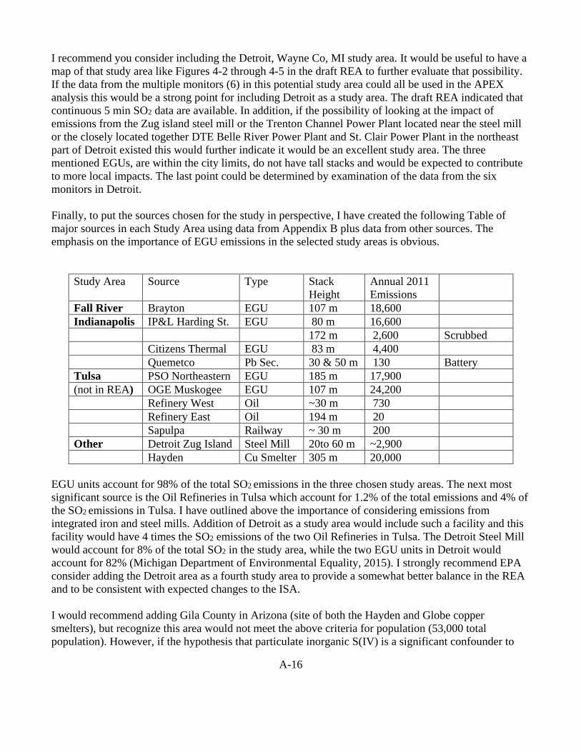
A-16

I recommend you consider including the Detroit, Wayne Co, MI study area. It would be useful to have a

map of that study area like Figures 4-2 through 4-5 in the draft REA to further evaluate that possibility.

If the data from the multiple monitors (6) in this potential study area could all be used in the APEX

analysis this would be a strong point for including Detroit as a study area. The draft REA indicated that

continuous 5 min SO2 data are available. In addition, if the possibility of looking at the impact of

emissions from the Zug island steel mill or the Trenton Channel Power Plant located near the steel mill

or the closely located together DTE Belle River Power Plant and St. Clair Power Plant in the northeast

part of Detroit existed this would further indicate it would be an excellent study area. The three

mentioned EGUs, are within the city limits, do not have tall stacks and would be expected to contribute

to more local impacts. The last point could be determined by examination of the data from the six

monitors in Detroit.

Finally, to put the sources chosen for the study in perspective, I have created the following Table of

major sources in each Study Area using data from Appendix B plus data from other sources. The

emphasis on the importance of EGU emissions in the selected study areas is obvious.

Study Area Source Type Stack

Height

Annual 2011

Emissions

Fall River Brayton EGU 107 m 18,600

Indianapolis IP&L Harding St. EGU 80 m 16,600

172 m 2,600 Scrubbed

Citizens Thermal EGU 83 m 4,400

Quemetco Pb Sec. 30 & 50 m 130 Battery

Tulsa PSO Northeastern EGU 185 m 17,900

(not in REA) OGE Muskogee EGU 107 m 24,200

Refinery West Oil ~30 m 730

Refinery East Oil 194 m 20

Sapulpa Railway ~ 30 m 200

Other Detroit Zug Island Steel Mill 20to 60 m ~2,900

Hayden Cu Smelter 305 m 20,000

EGU units account for 98% of the total SO2 emissions in the three chosen study areas. The next most

significant source is the Oil Refineries in Tulsa which account for 1.2% of the total emissions and 4% of

the SO2 emissions in Tulsa. I have outlined above the importance of considering emissions from

integrated iron and steel mills. Addition of Detroit as a study area would include such a facility and this

facility would have 4 times the SO2 emissions of the two Oil Refineries in Tulsa. The Detroit Steel Mill

would account for 8% of the total SO2 in the study area, while the two EGU units in Detroit would

account for 82% (Michigan Department of Environmental Equality, 2015). I strongly recommend EPA

consider adding the Detroit area as a fourth study area to provide a somewhat better balance in the REA

and to be consistent with expected changes to the ISA.

I would recommend adding Gila County in Arizona (site of both the Hayden and Globe copper

smelters), but recognize this area would not meet the above criteria for population (53,000 total

population). However, if the hypothesis that particulate inorganic S(IV) is a significant confounder to

A-17

SO2 exacerbation of asthma is shown to be correct, addition of Gila County as an additional study site

should be addressed. The importance of addressing a site with emissions from an integrated iron and

steel mill would also increase if this were the case. EPA is now examining older epidemiological data to

test this hypothesis in their preparation of the next versions of the ISA.

Description of Study Areas

The first draft REA included useful maps describing the study areas, e.g. Figures 4.2 through 4.5 of that

documents. These figures provided the following information which informed the reader about the study

area:

• A readable map of the area.

• The location of the SO2 monitors in the area, including an indication of whether the monitoring

site provided 5 min data.

• The location and size of various SO2 sources in the area.

• Relative equal distances from each of the sources.

I would recommend that similar figures be added to this version of the REA. In addition, addition of the

identification of the type of each source, like that given in Figures 3.1 – 3.3 of this version would be

valuable. This information would allow ready identification of the locations of monitors and sources for

the various Tables given in Chapter 3.

I am confused by Table 3.1. It indicates there was no monitor with continuous 5-minute data in

Indianapolis. How then was the study area modeled? Is the Table in error?

Charge Question 5. Does the Panel find the description of the air quality modeling done to estimate the

spatial variation in 1-hour concentrations (section 3.2) to be technically sound and clearly

communicated?

The steps required to provide needed input to AIRMOD are clearly laid out at the start of Chapter 3. I

am not a modeler and will not attempt to evaluate the use of the model, only to give my impression of

the methods used to provide data input to the model and seek input from other members of the panel

with expertise in the areas related to those questions.

Ground meteorological data. Fall River is the only study area without an airport in the study area. EPA

has used data from Providence to provide the wind data. Providence is 20 miles away and there is

possible influence from the bays in the region. In particular, the winds may be to the west on the

Providence side, but will tend to be from the east on the Falls River side. Do meteorologists in the panel

feel comfortable with the use of the Providence data?

Classification of Brayton as “rural” (Page 3-8, line 20). The stacks at Brayton were not “tall”, only 107

m high. Does the classification as “rural” in the model based on this assumption effect the AIRMOD

results? I have already commented on how the high emissions, low stack and wind rose data all point to

an expected high impact at Fall River.

A-18

Charge Question 6. To simulate air quality just meeting the current standard, we have adjusted model

predicted 1hour SO2 concentrations using a proportional approach focusing on the primary emissions

source in each area to reduce the modeled concentrations at the highest air quality receptor to meet the

current standard (section 3.4). Considering the goal of the analyses it to provide a characterization of

air quality conditions that just meet the current standard and considering the associated uncertainties,

what are the Panel’s views on this approach?

I have no comments on this section.

Charge Question 7. A few approaches were used to extend the existing ambient air monitoring data to

reflect temporal patterns in the study area (section 3.5). Does the Panel find the approaches used below

to be technically sound and clearly communicated? a. Data substitution approach for missing 1-hour, 5-

minute maximum, or 5-minute continuous ambient air monitor concentrations (section 3.5.1). b.

Estimating pattern of within-hour 5-minute continuous concentrations where 1-hour average and 5-

minute maximum are known (section 3.5.2). c. Combining pattern of continuous 5-minute concentrations

within each hour from monitors in or near the study area with the modeled 1-hour concentrations

(section 3.5.3).

Indianapolis: There were only maximum 5 min concentrations available at the single monitor at this

study area. You chose Detroit data to represent the hourly pattern at Indianapolis and used data from one

of the six monitors there. You have given no justification for the choice of the 1 of 6. A map for Detroit

like those for Figures 4-8 through 4-11 in the previous draft would help us evaluate the wisdom of that

choice. Please provide that to the panel. I consider the information presented on assumptions too

incomplete to reach a conclusion on the results from using the Detroit data.

Fall River: Good coverage of 5-minute data for 2011 and 2012 lends credibility to the data for these two

years and the tight statistics for these data in Table 3-10. I will leave it to modelers in the group to judge

how well the 2013 results are consistent with the first two years results. However, the results for Fall

River should be fairly solid based on the input data.

Tulsa: As indicated in Table 3-9, Tulsa had the most complete coverage of 5-minute data of any of the

study sites, with continuous 5-minute data at three sites for all three years and continuous data at a

fourth site added in 2013. However, there is not just a single coal burning EGU in the Tulsa area, but 2,

(http://www.powerplantjobs.com/ppj.nsf/powerplants1?openform&cat=ok&Count=500,

https://www.psoklahoma.com/global/utilities/lib/docs/info/facts/factsheets/PSO_Fact_Sheet_2015.pdf,

https://www.google.com/maps/d/viewer?mid=1Yf43pX6guhAx8Y_XZ7sy-

25CqUU&hl=en_US&ll=36.10870952767214%2C-96.17040100000003&z=9).

http://www.sourcewatch.org/index.php/Muskogee_Generating_Station. These include:

• Public Service Company of Oklahoma Northeastern Plant; 2 units with 856 MW capacity

burning natural gas and 2 Units with 936 MW capacity burning coal. The stacks for the coal fired

units are 185 m high and emit about 17,900 tons per year. The facility is located just south of

Oologah, OK, about 20 mi NE of the Holly Refinery. The monitoring station M0078 in figure

6.2 is located between Tulsa and the facility, being closest to the facility.

http://www.powerplantjobs.com/ppj.nsf/powerplants1?openform&cat=ok&Count=500

https://www.psoklahoma.com/global/utilities/lib/docs/info/facts/factsheets/PSO_Fact_Sheet_2015.pdf

http://www.sourcewatch.org/index.php/Muskogee_Generating_Station

A-19

• OG&E Muskogee Generating Station, 3 units with 1716 MW capacity burning coal. The stacks

for the coal fired units are 107 m high and emit about 22,409 tons per year. This facility is in

Muskogee, about 30 mi SE of the Holly Refinery.

It seems to me to be essential that the OG&E EGU be included in the analysis of the Tulsa data,

Figure 3-4. Ultimately the proof of the pudding for Section 3.5 is given in this Figure. It is not stated (or

clear) for which site this comparison applies. I suspect it is 2011 and 2012, Fall River. If this is so what

do the top two plots for 2013 look like where continuous 5-min data were not available? The statement

is made on page 3-26 that comparisons for Indianapolis were “similar.” Given the more indirect nature

of the Indianapolis analysis, please show us a similar Figure for Indianapolis. Finally, there were

continuous 5-minute data at all monitor sites for Tulsa, so estimation of 5-minute data from other

considerations was not needed. What do the plots for Tulsa look like, particularly, how much is the

scatter in the measured and predicted 5-minute data reduced? These key results would allow a more

definite evaluation of what is done in Section 3.5.

Reference

Michigan Department of Environmental Quality 20 August 2015. “Proposed Sulfur Dioxide One-Hour

National Ambient Air Quality Standard State Implementation Plan”,

http://www.deq.state.mi.us/aps/downloads/SIP/SO2SIP.pdf

Comments Prior to the April 20 Phone Call

9 April 2018 (Revised 26 April)

To members of the committee:

I am writing this note to the committee prior to the phone call because I have been advised by Aaron

Yeow that call will be the last of the panels activities in connection with the SO2 review.

The focal point of my comments is material added to the ISA in connection with advice from the

committee. It touches only on the parts of the ISA where I have had major input with my viewpoints on

SOs chemistry and the possible importance of emissions from smelters and integrated iron and steel

mills, and on major recommendations to EPA in connection with our last review of the ISA.

Specifically, it touches on the following from the June 30, 2017 letter to Administrator E. Scott Pruitt in

connection with the chapter on atmospheric chemistry and ambient air concentrations. In that letter we

made (among others) the following recommendations:

“To improve this chapter, emission trends from 2011-2016 should be added. It is also important to

highlight the contributions of emissions from smelters and integrated steel mills as these may explain

some high values in the data shown. The importance of pollution sources and the formation of other

sulfur compounds such as inorganic and organic particulate S(IV) and organic S(VI) species should be

discussed.”

A-20

The final Revised ISA was released by EPA in December 2017

https://cfpub.epa.gov/ncea/isa/recordisplay.cfm?deid=338596. However, notification of the release was

not send to the panel and we will not further review the document.

1. There are comments which follow which I have on each of the items in the quote from the letter to the

administrator given above. However, my major concern is with the treatment of literature related to

particulate sulfur(IV) compounds in the Final ISA and the implications for this atmospheric chemistry in

the treatment of the importance of emissions from smelter and integrated iron and steel mills in the REA

which we will discuss on April 20.

I have attached my past comments related to this chemistry and the REA (from my April 29, 2017 final

comments on the draft REA) below.

EPA has referenced the chemistry of inorganic S(IV) in particulate matter in the Final ISA (it was

completely missing from previous drafts). In section 2.3.3. of the Final ISA they cover the question of

particulate inorganic S(IV) in emission from smelters and integrated iron and steel mills as follows:

“Particle-phase inorganic and organic sulfur compounds have been identified in early studies (Eatough

and Hansen, 1983, 1980; Lee et al., 1980; Eatough et al., 1979; Eatough et al., 1978; Smith et al., 1976).

These studies identified inorganic SO32− complexed with Fe(III) in the particles emitted by a smelter

near Salt Lake City, UT. In a detailed spectroscopic study of the transient complexes that form between

SO2, a source of S(IV) in particles, and Fe(III) in the aqueous phase, Kraft and van Eldik (1989a) and

Kraft and van Eldik (1989b) reported that the oxidation of S(IV) by Fe(III) to form SO42− occurs on the

order of seconds to minutes and is further accelerated by low pH. Sulfuric acid is well known to absorb

water at even low ambient relative humidity (Seinfeld and Pandis, 2006). The highly acidic aqueous

conditions that arise once smelter plume particles equilibrate with the ambient atmosphere ensure that

S(IV)-Fe(III) complexes have a small probability of persisting and becoming a matter of concern for

human exposure.”

This summary does not consider the following from the peer reviewed literature, and which was

provided to EPA in my comments (references are from the material in my previous comments given in

the Appendix):

Our studies on inorganic S(IV) in aged plume particles come from the study of plumes from a copper

smelter, a coal-fired power plant study and an oil-fired power plant. In these studies, the presence of

inorganic S(IV) species was identified in both fresh and aged plumes and were found in the plumes of

the copper smelter and coal-fired power plant for the relatively long transport times (hours) (Eatough et

al, 1982, Eatough et al. 1981a). For the copper smelter plume studied the ratio of the inorganic S(IV) to

As increased with plume travel time. Average concentration of the inorganic S(IV) after about four

hours of plume travel was about 60% of the particulate sulfate. The data indicated (Eatough et al., 1982)

that the formation of stable particulate inorganic S(IV) involved chemical equilibria among the Fe plus

Cu aerosol content, aerosol acidity and the concentration of SO2(g), with the net result that after one or

two hour he amount of SOX present as stable particulate inorganic S(IV) increased with time, rather than

decreasing to near zero as assumed in the EPA Final ISA. For the coal-fired power plant plume, again

the amount of inorganic S(IV) relative to total SOX increased with plume travel time and after about 4

hours of plume travel was about 50% of the particulate sulfate. We also conducted a plume study of an

oil-fired power plant plume (Eatough et al, 1981a). Particulate inorganic S(IV) was not detected in the

https://cfpub.epa.gov/ncea/isa/recordisplay.cfm?deid=338596

A-21

primary emissions or plume of the oil-fired power plant. We also studied the chemistry of the formation

of sulfate and organic S(IV) and S(IV) compounds in these plume studies. Note that these plume studies

are not referenced in the Final ISA but the assumption of non-existence of plume particulate inorganic

S(IV) is assumed to be negligible as stated in the material in the Final ISA quoted above. In addition,

we have also reported on the laboratory generation of stable Fe(III)-S(IV) aerosol (Hilton et al, 1979).

This study is also not quoted. The metals which appear to be associated with the inorganic S(IV) as

outlined in the above referenced studies include Fe, Cu and Zn. The assertion that inorganic S(IV)

particulate material has “a small probability of persisting and becoming a matter of concern for human

exposure” is simply not supported by the peer reviewed literature.

The importance of this incomplete review of plume inorganic S(IV) particulate material with respect to

the REA is that EPA can assume that emissions from smelters and integrated iron and steel mills cannot

be of special concern.

2. We also requested that in the revision of the ISA the emission trends from 2011-2016 should be

added. That was not done. But this exclusion, from my point of view, does not seriously affect the

revised ISA in the same way the mistreatment of the literature mentioned above does.

3, We also requested that “It is also important to highlight the contributions of emissions from smelters

and integrated steel mills as these may explain some high values in the data shown.”

This point is more important than item 2. with respect to the development of the REA because it bears

on decisions made in selection of the study areas in that document.

The intent of this request is not covered in the Final ISA. The Final ISA does give the total emissions

from copper smelting and combined iron and steel mill facilities on the top of page 2-5. However,

consideration of the importance of smelter and iron and steel mill emissions could have been

highlighted, but were not in connection with the follow Figures, Figure 2-3 (this is probably the most

important because identifying the location of these facilities in this or a similar figure would have meet

our intent), Figure 2-13 (There is an integrated iron and steel mill within Cleveland. It could impact the

ambient monitors in the city. The effect seems to be as large as any influence of the RGUs to the east or

west of the city). Figure 2-18 and Table 2-12 do meet the intent of this request.

The request is important because it could have guided the decisions on selection of study areas in the

REA.

Observation

The result of the incomplete treatment of the plume presence of particulate inorganic S(IV) in plumes is

that the incorrect assumption that “The highly acidic aqueous conditions that arise once smelter plume

particles equilibrate with the ambient atmosphere ensure that S(IV)-Fe(III) complexes have a small

probability of persisting and becoming a matter of concern for human exposure” allows EPA to not

focus on the consideration of emissions from smelters and integrated steel mills, The importance of this

omission lies in the possible importance of these particulate inorganic S(IV) species as modifiers on the

effect of SO2 on asmathics. I have outlined the potential

A-22

Importance of this in the material final comments on the Draft IRP given in the Appendix where I have

suggested EPA should conduct an evaluation of past literature smelter based epidemiological studies to

determine if the stable inorganic S(IV) species may be effect modifiers of asthma for exposed

populations.

This suggestion is based on the early laboratory studies of Amdur (1971) and Alarie (1973) which

indicated that exposure to both SO2 and metal oxides present in smelter emissions resulted in an

enhanced animal response and that the resulting aerosols were irritating. I have suggested to EPA that a

possible fruitful set of data to evaluate the relative importance of aerosol S(IV) species associated with

smelter emissions would involve past epidemiological studies from about two to three decades ago when

smelter emission were much more significant, for example from the TX smelters in El Paseo (ASARCO

Cu smelter, closed in 1999), and Corpus Christi (ASARCO Pb smelter, closed in 1985), Az smelters

(ASARCO Cu smelter in Hayden, currently operating and Phelps Dodge Cu smelter in Douglas, closed

in 1987), from the Kennecott Cu smelter in Magna, UT prior to construction of the tall stack, from the

Tacoma WA smelter (American Smelting and Refining, a Cu smelter specializing in high As ore

refining, closed in 1985), or the smelters in Montana (ASARCO Pb smelter in East Helena, closed in

2001, Anaconda Cu smelter in Anaconda, closed in 1981) and Idaho (Bunker Hill Pb smelter in Kellogg,

closed in 1982). I know that several epidemiological studies were conducted at these locations, but I am

not familiar with the results of these studies with respect to asthma exacerbation. I recommended that

EPA look at this older data to see if an estimate of the relative potency of SO2 and smelter associated

aerosol S(IV) species can be determined. There will not be data on the concentrations of S(IV) in the

aerosols emitted from these sources, so total particulate exposure might need to be used as a surrogate.

.

If EPA does not conduct this exercise and the possible importance of exposure to particulate inorganic

S(IV) species, the possible importance of emission from smelters and integrated iron and steel mills, and

possible effect modifying of asthma exposure estimates due to the presence of fine particulate inorganic

S(IV) species will all remain unexamined and unknown.

Appendix

The following is from my April 29, 2017 final comments on the Draft IRP and relates directly to

my comments on the Final ISA as summarized above”

Relationship to Sources:

A potentially enlightening exercise might be to examine if any relationship exists between the results of

epidemiological studies and the source of SO2 for a given epidemiological study. I suggest this because

it might enlighten whether particulate S(IV) (e.g. absorbed SO2) might be important in exacerbation of

asthma. This suggestion is based on the early laboratory studies of Amdur (1971) and Alarie (1973)

which indicated that exposure to both SO2 and metal oxides present in smelter emissions resulted in an

enhanced animal response and that the resulting aerosols were irritating. Postulating that the work of

Amdur might reflect the present of stable metal sulfite species in the aerosols studied, and that the

formation of such aerosol species, rather than aerosol sulfate, might explain the results of the EPA

CHESS study in the Salt Lake City environment with substantial impact from Cu smelter emissions

(EPA 1974), we conducted studies on S(IV) associated with ambient aerosols. This work demonstrated

that stable transition metal ion - sulfite species existed in aerosols associated with smelter emissions

A-23

(Smith 1976, Eatough 1979, Eatough 1980) and could be formed in aging smelter plumes (Eatough

1981a, Eatough 1982). The sulfite species were present at from 10 to 30 mol % of the sulfate species in

the smelter associated aerosols. The sulfite species were less important in urban or coal-fired power

plant plumes (Eatough 1978). We also demonstrated that stable Fe(III) –S(IV) aerosols could be

routinely generated in the laboratory (Hilton 1979). The measurement, stability and formation of these

inorganic S(IV) species in aerosols has been reviewed (Eatough 1983). These S(IV) species were

present in emission from all smelters studied, were present in lower amounts in emissions from coal-

fired power plants and additional material was formed during plume transport in smelter plumes. The

amount of the S(IV) species, relative to sulfate average 0.1 mol S(IV)/mol sulfate in the coal fired power

plant plumes and 0.5 mol S(IV)/mole sulfate in aged smelter plumes. The formation of S(IV) in smelter

plumes increased with decreasing acidity of the aerosol.

If these S(IV) containing aerosols identified in the above reviewed research account for the enhanced

effect of SO2 in the presence of transition metal containing aerosols in animal exposure studies, then this

class of compounds may be important in the interpretation of the morbidity effects associated with

exposure to pollution from refinery sources. A careful review of pertinent epidemiological literature

may inform this postulate.

The current set of counties which are nonattainment with respect to the current SO2 NAAQS will

probably not provide the needed information. A review of nonattainment counties with populations near

or over 100,000 shows that with two exceptions, the SO2 exposures are dominated by emissions from

coal-fired power plants, where aerosol S(IV) species are less important. The two exceptions are

Jefferson County, MO where about 30% of the SO2 emissions currently are from the Herculaneum Lead

Smelter, with the remainder being from coal-fired power plants, and the Steubenville, Weirton region in

eastern Ohio and western Pennsylvania, where emission from the Weirton Steel are likewise, a minor

portion of the SO2 emissions in the immediate area, with coal fired power plants being more important.

These two locations would only stand out from the other nonattainment areas if the morbidity influence

of aerosol S(IV) species was much greater that that associated with SO2 itself. In addition to being a

nonattainment area, Jefferson County, MO was also highlighted in the September 2008 Integrated

Science Assessment for Sulfur Oxides, but with no epidemiological discussion associated with this

nonattainment area (part of the St. Louis MO MSA).

Probably a more fruitful set of data to evaluate the relative importance of aerosol S(IV) species

associated with smelter emissions would involve past epidemiological studies from about two to three

decades ago when smelter emission were much more significant, for example from the TX smelters in

El Paseo (ASARCO Cu smelter, closed in 1999), and Corpus Christi (ASARCO Pb smelter, closed in

1985), Az smelters (ASARCO Cu smelter in Hayden, currently operating and Phelps Dodge Cu smelter

in Douglas, closed in 1987), from the Kennecott Cu smelter in Magna, UT prior to construction of the

tall stack, from the Tacoma WA smelter (American Smelting and Refining, a Cu smelter specializing in

high As ore refining, closed in 1985), or the smelters in Montana (ASARCO Pb smelter in East Helena,

closed in 2001, Anaconda Cu smelter in Anaconda, closed in 1981) and Idaho (Bunker Hill Pb smelter

in Kellogg, closed in 1982). I know that several epidemiological studies were conducted at these

locations, but I am not familiar with the results of these studies with respect to asthma exacerbation. I

recommend that EPA look at this older data to see if an estimate of the relative potency of SO2 and

smelter associated aerosol S(IV) species can be determined. There will not be data on the

concentrations of S(IV) in the aerosols emitted from these sources, so total particulate exposure would

A-24

need to be used as a surrogate. The importance of elucidating the effect of these exposures is correctly

alluded to in the ISA on Page 4-12, Line 11.

Organic Oxysulfur Compounds in the Atmosphere

This section was added to my preliminary comments to provide a written response to the question raised

in the preliminary comments by Dr. Daniel Jacob. Compounds identified by BYU and discussed below

include:

Alkyl Sulfates. We have previously identified monomethyl sulfuric acid and dimethyl sulfate in power

plant plumes (Lee 1980, Eatough 1981b, Hansen 1987)) and in the Los Angeles Basin (Eatough 1986,

Hansen 1986). The alkyl sulfates have been shown to be present in emissions from both coal and oil-

fired power plants (Eatough 1981b). In addition, formation of dimethyl sulfate during plume transport

has been seen in the plumes of both a oil-fired and a coal-fired power plant (Hansen 1987). Dimethyl

sulfate did not form in the plume of the oil-fired power plant studied while it resided in a fog bank, but

formation was seen after the plume exited the fog bank. The rate of conversion of SO2 to dimethyl

sulfate was about 0.4 mole %/hr in the oil fired power plant plume and about 0.05 mole %/hr in the coal

fired power plant plume. Particulate phase dimethyl sulfate dominated in these two studies. In the Los

Angeles Basin studies (Eatough 1986) dimethyl sulfate was only seen in air masses not imbedded in a

fog bank, i.e. generally in the inland area. Gas phase dimethyl sulfate was the dominate species in these

studies, was present at highest concentrations in transported plumes in the Inland Empire and was seen

to exceed 10 mole % of the total sulfur oxides present. It should be pointed out that at the time of these

studies, substantial SO2 emission from power plants were present in the Basin..

Dimethyl sulfate is a mutagen and suspected human carcinogen, so it’s presence may be important with

respect to toxic species, but I am not aware of any data indicating that inhalation will exacerbate asthma.

Bis Hydroxymethyl Sulfone.

Several different methods of analysis of particulate samples collected from the plumes of coal-fired

power plants or from areas heavily impacted by coal-fired boilers indicated that a S(IV) compound

distinctly difference form inorganic S(IV) was present in the samples (Eatough 1978, Eatough 1981,

Richter 1981). This compound was subsequently identified as bis-hydroxymethyl sulfone (Eatough

1984). The sulfone was usually present in emissions from coal- or oil-fired power plants at mol ratios of

about 0.5 (range of 0.1 to 1.0) compared to sulfate (Eatough 1983). First order formation of the sulfone

was observed in plumes from six different power plants at rates of from 0.4 to 3.0 % SO2/hr. with the

observed rate being inversely proportional to atmospheric water partial pressure (Eatough 1983). The

sulfone was found in highest concentrations in the Las Angeles Basin in inland samples (mol fraction

comparable to sulfate), but was not seen in coastal samples impacted by fog or clouds (Farber 1982).

A-25

Toxicological data is not available for bis-hydroxymethyl sulfaone.

Other Organic Oxysulf Comounds.

Aerosol phase methane sulfonic acid (Panter 1980) and gas phase ethylene sulfite (Jones 1974) have

been identified in atmospheres impacted by emission from coal fired power plants, but only at

concentrations much less than the above described species.

References

Alarie Y., Wakisaka I. Oka S. (1973) “Sensory Irritation by Sulfite Aerosols,” Environ. Physiol.

Biochem., 3, 182-184.

Amdur M.O. (1971) “Aerosols Formed by Oxidation of Sulfur Oxide.” Arch. Environ. Health, 23, 459-

468.

Eatough D.J., White V.F., Hansen L.D., Eatough N.L. and Cheney J.L. (1986) "Identification of Gas-

Phase Dimethyl Sulfate and Monomethyl Hydrogen Sulfate in the Los Angeles Atomsphere," Environ.

Sci. Technol., 20(9), 867-872.

Eatough D.J. and Hansen L.D. (1984) "Bis-Hydroxymethyl Sulfone: A Major Aerosol Product of

Atmospheric Reactions of SO2(g)," Sci. Total Environ., 36, 319-328.

Eatough D.J. and Hansen L.D. (1983) "Organic and Inorganic S(IV) Compounds in Airborne Particulate

Matter," in Trace Atmospheric Constituents: Properties, Transformations and Fates, 12, S.E. Schwartz,

ed., John Wiley and Sons, New York, NY 221-268

Eatough D.J., Christensen J.J., Eatough N.L., Hill M.W., Major T.D., Mangelson N.F., Post M.E., Ryder

J.F., Hansen L.D., Meisenheimer R.G. and Fisher J.W. (1982) "Sulfur Chemistry in a Copper Smelter

Plume," Atmos. Environ., 16, 1001-1015.

Eatough D.J., Richter B.E., Eatough N.L., and Hansen L.D. (1981a) "Sulfur Chemistry in Smelter and

Power Plant Plumes in the Western U.S.," Atmos. Environ., 15, 2241-2253.

Eatough D.J., Lee M.L., Later D.W., Richter B.E., Eatough N.L. and Hansen L.D. (1981b) "Dimethyl

Sulfate in Particulate Matter from Coal- and Oil-Fired Power Plants," Environ. Sci. Tech., 15, 1502-

1506.

Eatough D.J. and Hansen L.D. (1980) "S(IV) Chemistry in Smelter Produced Particulate Matter," Amer.

J. Indus. Med., 1, 435-448.

Eatough D.J., Eatough N.L., Hill M.W., Mangelson N.F., Ryder J., Hansen L.D., Meisenheimer R.G.

and Fischer J.W. (1979) "The Chemical Composition of Smelter Flue Dusts," Atmos. Environ., 13, 489-

506.

A-26

Eatough D.J., Major T., Ryder J., Hill M., Mangelson N.F., Eatough N.L., Hansen L.D., Meisenheimer

R.G. and Fischer J.W. (1978) "The Formation and Stability of Sulfite Species in Aerosols," Atmos.

Environ., 12, 263-271.

EPA (1974) “Health Consequences of Sulfur Oxides: A Report from CHESS, 1970-1971” EPA-650.1-

74-004, May 1974

Farber R.J., Huang A.A., Bregman L.D., Mahoney R.L., Eatough D.J., Hansen L.D., Blumenthal D.L.,

Keifer W.S. and Allard D.W. (1982) "The Third Dimension in the Los Angeles Basin," Sci. Total

Environ., 23, 345-360.

Hansen L.D., Eatough D.J., Cheney J.L. and Eatough N.L. (1987) "The Formation of Dimethyl Sulfate

in Power Plant Plumes," 80th Annual Meeting of the Air Pollution Control Association, Paper No. 87-

96.3, New York, New York, 21-26 June.

Hansen L.D., White V.F. and Eatough D.J. (1986) "Determination of Gas-Phase Dimethyl Sulfate and

Monomethyl Hydrogen Sulfate," Environ. Sci. Tech., 20(9), 872-878. [362

Hilton C.M., Christensen J.J., Eatough D.J. and Hansen L.D. (1979) "Fe(III)-S(IV) Aerosol Generation

and Characterization," Atmos. Environ., 13, 601-605.

Jones P.W. (1974) Proceedings of the 1974 APCA Meeting, Paper No. 74-25.

Lee M.L., Later D.W., Rollins D.K., Eatough D.J. and Hansen L.D. (1980) "Dimethyl and Monomethyl

Sulfate: Presence in Coal Fly Ash and Airborne Particulate Matter," Science, 207, 186-188.

Panter R. and Penzhorn R.D. (1980) “Alkyl Sulfonic Acids in the Atmospheere”, Atmos. Environ., 14,

149-151.

Richter B.E. (1981) “S(IV) and Alkylating Agents in Airborne Particulate Matter,” Ph.D. dissertation,

Brigham Young University, Provo, UT.

Smith T.J., Eatough D.J., Hansen L.D. and Mangelson N.F. (1976) "The Chemistry of Sulfur and

Arsenic in Airborne Copper Smelter Particulates," Bull. Env. Contamination and Toxicology, 15, 651-

659.

A-27

Dr. H. Christopher Frey

Chapter 4




The general underlying approach seems to be reasonable, but is not well explained here. The description

needs extensive revisions. See detailed comments below for pages 4-2 through 4-15 for particulars.


This section does not do a very good job of explaining, justifying, and interpreting the approach used for

elevated ventilation rate. This section, as all others in this chapter, needs extensive copy editing. The text

would also benefit from being more formal, more specific, more precise, and more detailed, which

would make it clear. This section needs more details on goodness of fit and other indicators of validity

and model prediction error of of Equation 4-3. The material on elevated breathing rate is terse and there

is no evaluation of the suitability or goodness-of-fit of this approach. I would characterize this section as

in need of major revisions.


See detailed comments below for pages 4-16 to 4-20. This section is missing an adequate justification

for focusing on only five microenvironments. I agree that this is a suitable approach, but it is not

sufficiently explained. In part, the lack of quantitative identification of the contribution of different

microenvironments to peak exposures makes the text seem vague and subjective. If possible, the text

should be quantitative regarding the fraction of peak exposures from previous analyses (or this analysis)

that are from each microenvironment. Stronger quantitative support for claiming that the majority of

peak exposures are related to outdoor microenvironments would be helpful. As noted in the detailed

comments, the selected microenvironment for vehicles seem intuitively obvious but a rationale for

including it has not been articulated. It would help to know if this represents personal vehicles or if it is

somehow intended to represent all types of vehicles. Likewise, for indoor-other, more clarity on the

purpose, key microenvironment, and choices made to quantify this microenvironment are needed. For

example, given the focus on children as one key sensitive subpopulation, why is the school

microenvironment not considered when developing input data for indoor-other? Or, by what reasoning

and based on what data is a judgment supportable that office and school have similar ventilation

characteristics?

Also missing here is consideration of the two different air quality scaling methods used to estimate air

quality consistent with the current standard. This aspect of the analysis study design needs to be

introduced and explained.

A-28

There appears to be misuse of the term “penetration factor” and lack of clarity and interpretation on

some other points as detailed below.

d. Derivation of the exposure-response functions (section 4.5.2).

See also detailed comments on pages 4-25 to 4-27.

This section is a relatively minimalist treatment of the topic. In general, for any kind of curve fitting

using regression, there should be a discussion of what functional forms and parameterizations were

identified and compared, and which one(s) were selected, and why, for fitting and evaluation. There

should be a systematic approach to model evaluation that takes into account statistical factors, such as

goodness-of-fit metrics, and whether the model formulation is appropriate relative to the type of data

and its characteristics, as well as regarding the biological plausibility of the inferred relationships. The

precision and accuracy of the fitted model versus calibration data, and, if possible, evaluation of

precision and accuracy for out-of-sample data (validation), would be important to include. The 95%

interval for the mean is a confidence interval, not a prediction interval. The prediction interval would be

the 95% frequency range of the model prediction.

The probit regressions given in Figure 4-1 may well be suitable but they are not adequately motivated or

evaluated in the text. For example, why was probit regression selected?

Other General Comments

The writing style of this chapter needs to be substantially revised. It is written in a somewhat informal,

breezy manner, with vague or ambiguous language and curious mixture of irrelevant specifics as well as

omissions of needed details. The status of the writing is somewhat disappointing, since there have been

similar chapters regarding exposure modeling in REAs from prior reviews not just for SO2 but also CO,

NOx, and O3. At this point, some of the key points can be fairly standardized and do not require de novo

writing. However, since it is not the role of CASAC to correct poor writing, the comments here focus on

technical issues.

The Policy Assessment does a better job than this REA in terms of clearly identifying the ways in which

the current assessment is improved compared to the last review. Specifically, since the last review, the

exposure assessment has been updated in the following important ways:

▪ Expanded CHAD

▪ Updated NHANES data

▪ Updates to the algorithms used to estimate resting metabolic rate

▪ Updates to the ventilation rate algorithm

▪ Updated population demographic data

▪ Analysis for a three year simulation period consistent with the form of the current

standard

▪ Air quality data based on more recent emissions and circumstances since the 2010

revision of the standard.

Although most of these points are addressed in the REA, they are not addressed in a sufficiently clear

and organized manner. Furthermore, the implications of these changes and updates are not adequately

discussed or interpreted.

A-29

Detailed Comments

• Page 4-1, line 5: “health effects information” is vague. This term is used in several places (e.g.,

again on page 4-2, line 1) but is not clearly defined. What specific “information”?

• Bottom of page 4-1 and top of page 4-2. It seems strange not to indicate that the simulation of

population distributions is based on simulation of inter-individual variability in exposure (i.e.

cross-section) and temporal variability in exposure for a given individual. The latter is sometimes

referred to as intra-individual variability.

• 4-2/5-6: the idea that these individuals are simulated based on frequency distributions for model

inputs is not conveyed clearly.

• 4-2, line 7: the word “though” is used repeatedly in this chapter. It is not the correct coordinating

conjunction to use. Furthermore, consider breaking the compound sentences into two separate

sentences rather than linking them with a coordinating conjunction.

• 4-2/15: ‘distribution’ not ‘collection’

• 4-2/17: again, ‘distribution’ not ‘collection’

• 4-2/26-29. Not parallel - needs to be copy edited and rewritten.

• Section 4.1.1: why is the analysis based on census blocks rather than, say, census tracts. It

always helps to do more than just state what choice was made. The rationale for the choice

should be given. For example, is there really adequate data to quantify variability in exposure

concentrations among census blocks? What is the justification for this level of spatial resolution?

• 4-3/5-10: here and in other places, lists are given of APEX files. However, these files are not

well-explained nor is the need for listing them clear to the reader. Thus, if they are listed, explain

why they are listed (what is the purpose of this detail) and be more specific and clear as to what

they contain and the significance. Otherwise, it seems sufficient to explain what are the inputs to

APEX without getting into details of files. Such details can go in an appendix.

• 4-3/16: The word “calculate” is not really appropriate for a model that is making estimates based

on data subject to uncertainty. “Calculate” implies a high level of precision. A better word choice

is “estimate”. It is not clear HOW the ACS data are used to estimate the number of employed

people. Explain more clearly, with more detail.

• 4-3/21: please explain why it is necessary to quantify both the block and tract level – this is not

clearly explained and will not be self-evident to many readers.

• 4-3/23-24: not clear why this information is needed here. See earlier comment.

• 4-3/29: the text bounces between tracts and blocks, which is very confusing to the reader. Give a

paragraph, perhaps before Section 4.1.1, that explains the spatial resolution selected and explains

why both tracts and blocks are used in the same analysis.

• Page 4-4: in several places, the text refers to “population data.” However, this term is vague and

is not clearly defined. Defined, with specifics, after which this term should be used consistently.

• 4-4/3-6: at what geographic scale? Census tracts? This is another example of a compound

sentence whose length, along with breezy vague text, leads to ambiguity. Break this into three

sentences (asthma prevalence, ‘population data’, and income to poverty ratio). For each sentence,

make clear the spatial resolution, and the temporal characteristics (e.g., from what time period, at

what time resolution). In general, to be clear requires being more specific and not lumping too

many topics into a single sentence.

• 4-4/6: Explain why family income to poverty ratio is needed and how it was/will be used.

A-30

• 4-4/8: prevalence of what? Insert “asthma”. “Using this information, we….” This is vague.

HOW was it used? Be more specific. i.e. what were the key steps? How was income to poverty

ratio used, for example? What are the key equation(s) and their jusitification?

• 4-4/14: if the file is going to mentioned, state what it is for… i.e. insert ‘for asthma prevalance’.

But does this also include the income to poverty ratio data? Thus, is the file about more than just

prevalence? Not very clear.

• 4-4/19-21: very hard to parse this sentence. “considering” is vague. Exactly how was this

‘considered’?

• 4-4/22: what exactly was the “estimation approach” ? this has not been adequately explained.

• 4-4/24: The data in Table 4-1 contradict the statement that children have higher rates than adults.

E.g., the is not true for females in Indianapolis.

• 4-4/26: “By our…” is awkward.

• 4-5/5: “These … values”… implies that the values were previously stated. However, this is not

correct. The values given area aggregated summaries.

• Table 4-1: add a more useful indication of variability, such as the coefficient of variation or

standard deviation, or a 2.5 to 97.5 frequency range. Min and max range is less useful because it

can be subject to random fluctuation.

• Footnote to table 4-1 – how was this “derived” from the mentioned data?

• Table 4-1 and 4-2 are redundant. Cut one of them.

• 4-6, section 4.1.3: it would help the reader to add a sentence or two on whether/why commuting

is an important activity to include in the analysis. It is implied that the need for this is self-

evident, but instead the need or purpose for this should be explained. Also, the reader wonders

about whether or how commuting between blocks within a tract is handled.

• 4-7/8-9: For clarity, does this refer to inter-tract commuting? Presumably, inter-block commuting

within a tract is not simulated, but this point is not clear.

• 4-7/11-12: if file names are given, then be more specific as to their content. E.g., how are

“commuting times” given? Are they stratified in any way? Not clear.

• 4-7/21: the concept of a “conditional variable” needs to be explained clearly. Otherwise, this

term is undefined.

• 4-7/17-28: This is very hard to follow. This reads like a laundry list of input files but the basic

purpose and concepts related to these data have not been clearly defined. Thus, this is probably

not the right place for this list.

• 4-7/30: A reference is given to Appendix F. Appendix F seems to do a better job of describing

the APEX model than does this chapter. Although Appendix F dives into some details that aren’t

needed in the main paper, consideration should be given to elevating some of the information

from the Appendix to the main paper, to provide the reader with a better explanation of APEX.

For example, “METS distributions” is unclear at this point.

• 4.1.4.1 – before getting into status variables, it may help to first explain the choice of

microenvironments. This would avoid some confusion. For example, on p 4-8, line 4, when “car”

is mentioned, the reader wonders also about transit buses, and other transport modes. If a

decision has been made to bound some MEs out of the analysis, this would be helpful to know

before reading about status variables, so that the reader isn’t wondering about things that are

intentionally excluded.

• 4-8/7: need to break this into two sentences. These two clauses do not fit together.

• 4-8/1st paragraph. Not clear if air conditioning use prevalence is a status variable.

A-31

• 4-8/16: determined how? With regard to this paragraph, which are inputs? Which are inferred

and, if inferred, how?

• 4-8/27-28: seems like reverse causality – ventilation rate is related to energy expenditure, not the

other way around.

• 4-8/31: awkward wording.

• 4-9/2: what is “diverse” about this? Not clear.

• 4-9/19 or after – the effect of the “new algorithm” ( what really is new about it – is it the same

functional form with recalibrated parameter values?) should be mentioned… e.g., based on Table

10 in Appendix H, it seems that there isn’t much difference in predictions of RMR for the “New”

versus “Old” algorithm. This should be mentioned.

• 4-11/4-5: what is PROC TRANSREG?

• 4-11/19: give equation

• 4-11/24-25: is this meant to be a mean value? Is there variability or uncertainty in this value?

• 4-12/16: “somewhat”? unclear

• 4-12/21: WHY does APEX use only 55,000 of 180,000 person-days of diaries?

• 4-12/26: Not clear how these files “develop” activity patterns. Explain.

• 4/12/31: summary statistics such as what?

• 4-13/11: “this issue”? not clear. Individuals who have never had asthma is the immediate

antecedent. This paragraph ends with a run-on sentence, and in general is not well written.

• Section 4.1.5.1 I didn’t review this section because I am a co-author on the cited Che et al.

(2014) paper mentioned in this section.

• 4-16/28: location codes – are these microenvironments? Not very clear.

• 4-16/general… “work” is not given in Table 4-4. The general idea of limiting the analysis to a

few microenvironments is reasonable, but not enough is done here to explain this. The inclusion

of outdoor and near-road makes sense. Some rationale should be provided for why vehicle is

included. I don’t disagree that it be included, but there should be a reason for it – e.g., because

vehicle occupants typically receive higher exposure concentrations compared to other

microenvironments (based on some quantification). Residential makes sense since people spend

a lot of time in their residence. Indoor-other seems to be equated with work in the text but this is

not very clear. How much do these 5 microenvironments contribute to daily exposure? While it

may be that the “majority” of peak exposures occurred while outdoors, more quantitative support

should be given for this point.

• 4-17/1-6. What is a “relative location”? Ambient air “is drawn to calculate” ? doesn’t make

sense. It is not clear as to how tract-level ambient concentrations are quantified. This should be

explained. Later, in the REA, it is mentioned that APEX was apparently run for two different air

quality scenarios based on different methods for scaling air quality to just meeting the current

standard, but this aspect of the exposure modeling study design seems to be omitted in this

chapter.

• 4-17/24: this implies that the presence of AC and outdoor temperature are among variables for

which sufficient data are not available. Is this really the intended meaning? Also, what are the

“other variables” e.g., would this include characteristics of housing type, characteristics of the

building envelop, age of the building, etc? Even if not available, it would help to be clear

regarding what variables are known to be associated with variability in AER, and whether the

quantifiable variables are sufficient to adequately explain variability. Also, it is not clear why

“city” is an influential factor. It seems more logical that climate zone is an influential factor and

A-32

that city might be used as a surrogate for climate zone. Is there some other intended role of “city”

as a factor?

• 4-18/8: geographic region isn’t really the key factor here – it is climate zone.

• Tables 4-5 and 4-6. The tables are mentioned in the text but not interpreted or discussed. Some

justification/explanation is need for imposing minimum and maximum values on a lognormal

distribution – this can change the effective parameters of the distribution (e.g., the simulated

GSD will not be as large as the input GSD). Variability in AER among study areas, with respect

to temperature and between residences with and without AC should be interpreted, particularly to

the extent (if any) that this may be influential in simulation results.

• 4-19/5: use “dependent” rather than “conditioned”

• 4-19/7-11: this text is generally unclear. How exactly is prevalence different from usage? How

does AER represent AC usage? The last two sentences are very hard to understand.

• Section 4.2.3: seems to imply that office is used to represent “all other” – as such, a

rationale/justification should be given. Since children with asthma are a key sensitive group, why

is more attention not given to schools as an “other” microenvironment? Are offices and schools

similar with regard to AER and indoor exposure to ambient SO2 ?

• 4-20/18: the use of the term “penetration factor” seems incorrect here and in several places.

Commonly, penetration factor is part of the infiltration factor. Here, the intended meaning seems

to be the ratio of indoor to outdoor concentration (I/O ratio). Penetration factor is not the same as

the I/O ratio. See also line 30.

• 4-20/20-21: SO2 is far more soluble than NO2. Does this have implications for deposition or loss

processes in the indoor environment that are different than for NO2?

• 4-20/25: “broadly defined uniform distributions” is (a) vague and (b) implying multiple

distributions. For the latter, what do these distributions depend upon?

• 4-20/26-32: I/O ratio not penetration factor. Limited data – in what way? Indicate the sample size

or other characteristic that conveys the “limited data”. What is meant by “location” – is this

“study area” or census block? Be more specific.

• 4-21/6: “geographic area” not “size”

• 4-21/9: linear interpolation? (say so).

• 4-21/22: “estimated” not “derived”

• 4-22/1: above “specified,” not “varying”

• 4-22/4-13: Given how APEX is used in the PA, the choice of bins seems difficult to understand.

For example, why is there so much resolution for low concentration bins below 100 ppb? The

total number of bins would be helpful. e.g. 15 bins up to 150 ppb, 5 bins between 150 ppb and

250 ppb, and how many bins above 250 ppb? Is there some rationale for the varying choices of

bin widths and why there is much higher resolution (narrower ranges) for lower concentrations?

• 4-22/31: “information” is vague. Summaries of what quantities, more specifically?

• 4-23/12: “this information” refers to what? The antecedent is controlled studies. Doesn’t seem to

be correct or clear. The binning approach described previously does not appear to be harmonious

with the choice of benchmark concentrations given in this paragraph.

• Table 4-9 and more broadly in the text, the issue of oral versus nasal breathing needs some more

discussion. Although the point that many of the controlled experiment with low SO2

concentrations were based on oral breathing, whereas others were based on free-breathing is an

important consideration, it is also the case that at high ventilation rates there can be a transition

A-33

from nasal to oral breathing. Such a transition is typical of real-world behaviors and thus perhaps

should be discounted as readily as seems to be the case in this chapter.

• 4-25/1-2: replace “described” with “that correspond to.” Insert “as described” before “in the

second draft.”

• 4-28/23: it doesn’t make sense to say that algorithms account for variability in input data. Input

data are inputs to an algorithm. Perhaps the intended mean is that variability is accounted for in

input data, and is also quantified based on algorithms – but will need to say a bit more (at least

give an example).

• 4-29/7: “In any event,” ? delete this.

A-34

Dr. William Griffith

I would suggest clarifying in this chapter when you are calculating the number of people and when you

are calculating the number of simulated people. The early part of the chapter states your calculations are

for simulated persons (page 4-1 lines 17, 22, page 4-22 line 33) and that you chose to set the number of

simulated persons at 100,000 for each study area. Later in the chapter you alternate in describing the

calculations as being for the number of people (page 4-21 line 26, page 4-22 line 10, page 4-25 lines 4,6

and elsewhere) and number of simulated people without indicating when you have converted between

the two. The text should more clearly indicate when you switch between the two types of calculations.

The results in the text are presented only as the percent of asthmatics for the three study areas and never

as the number of asthmatics even though in Figure 2-1 (page 2-1) you indicate this is one of your main

Risk Metrics. I was hoping to see in the REA tables of the number of asthmatics responding due to SO2

exposures, which I think is an important way to communicate the results, but instead there are only

tables with the percentage of the asthmatic population affected.

I suggest that there be some discussion of the assumption made in the calculations that the asthmatics in

the human exposure studies were similar in their asthma to the people who answered that they had been

diagnosed with asthma in the National Health Interview Study.

I think the text would read more smoothly if you could move the names of the APEX files to footnotes,

or put the APEX files in an appendix and refer to the appendix in the text.

The Chapter would be easier to read if you had a table in the first part of the chapter that showed a brief

description of each of the simulations/formulas/calculations presented in the following sections to give

the reader a feeling for the overall flow of the chapter.

I found some of the text to be rather awkwardly stated because you appeared feel it necessary to repeat

some of the information given in previous sections. In some cases, the text in the Appendices seemed to

read more smoothly while not being appreciably longer, for example in parts of Appendix F.

This chapter (and Chapter 6 and the PA) should mention that it only deals with diagnosed and treated

asthmatics. There is a large population of untreated asthmatics and it is unknown if they respond in the

same manner to SO2 as the people in the human exposure studies.

The following are suggestions for potential improvements

• This chapter may need to clarify why children ages 0-4 years were not included in the risk

estimates. The text indicates that asthma prevalence data was available for children in this age

range. It does not provide any justification for only including children aged 5-19. Is their

additional material in the ISA that outlines reasons for this choice which could be referenced in

the REA text?

• The chapter may need additional information or references from other documents (such as the

ISA) about:

A-35

o The similarity of the participants between studies (Table 4-10) used in the derivation of

the Exposure-Response function. Did the studies use similar criteria for recruiting

subjects and for evaluating the severity of asthma?

o Why was the probit function used for the Exposure-Response function?

o Why differences between the studies in exposure duration and ventilation shown in Table

4-10 were not taken into account in deriving the Exposure-Response Functions?

P4-4 line 11-12 drop “using the 11-character… tracts and blocks.”

P4-4 lines 19-28 and p4-5 lines1-6 This paragraph is awkwardly written and needs to be rewritten and

shortened

P4-8 line 23 Since you give the coefficients you should give the units for BM and BSA, or you could

drop the formula and refer to Appendix F4.

P4-11 line 9 Since you give the regression parameters you should give the units for VE, VO2, and

VO2m.

P4-20 lines 14-15 Please give the units for AER.

P4-23 line 25-26 I am not sure why you characterize 10% as being a low percentage of asthmatics to

respond.

P4-25 lines 4-5 should this read “The REA assessment estimates the percent of the asthmatic population

expected to experience such a decrement,” and on lines 5-6 “total number of occurrences of these effects

per asthmatic individual”

P4-25 lines 15-16 should be “range of 5-minute and 10-minute SO2 concentrations.”

P4-25line 19 Check if these are actually prediction intervals. Also, I suggest to only plot the 95% upper

limit for prediction since the REA and PA do not use the 5% limit.

P4-25 line 20 should be “percent of asthmatic study populations.”

P4-26 Table 4-10 footnote b indicates that the half persons in the sRaw N columns are due to averaging.

In fitting the probit function did you take into account the averaging of the first and second rounds? The

statistical method used for dealing with the half persons should be referenced.

P4-27 line 3 should read “Percent of individuals in an asthmatic population” or something similar to

emphasize that this is not the general population. Also it would be clearer to label the y-axis in Figure 4-

1 as the “percent of Asthmatics” rather than “Percent of Population.”

Appendix J is not clear in Tables J10-J27 whether the “number of people” is the number of simulated

asthmatics or the number of asthmatics in the population. Also Appendix J does not give the regression

A-36

parameters for the probit Exposure-Response functions or the statistical method used for estimating the

probit functions when you averaged the first and second rounds of observations.

A-37

Dr. Steven Hanna

Note that my expertise is primarily in atmospheric transport and dispersion modeling, analysis of

observed concentrations, and uncertainty and variability, and my comments focus on those areas. I was

asked to comment on the areas related to Chapter 3 “Ambient Air Concentrations” and associated

Appendices A, C and D. In addition, I comment on Chapter 6 “Variability Analysis and Uncertainty

Characterization.”

Charge questions for the Panel’s consideration are presented below for Chapters 1, 2, 3 and 6. I assume

that Appendices A through D fall under Chapter 3 and include those appendices in my comments.


Charge Question 1. Does the Panel find the introductory and background material, including that

pertaining to previous SO2 exposure/risk assessments, to be clearly communicated and appropriately

characterized?

There is a tendency to assume that the reader is already familiar with the previous reviews of the

NAAQS for SOx and the various key issues. Since I joined this panel only about three years ago, much

of the previous decades of work has been sometimes puzzling to me, in the sense that it does not

conform to my research experiences. Surely it is possible to explain the key facts in a succinct way that

is understandable to most readers. I have a hard time finding exactly where the health end-points or

criteria are clearly defined in this chapter. Similarly, it would help if the new information covered in the

current REA could be more clearly explained. What is new and different here?

I find that there are many places in the procedure where subjective or arbitrary choices are made, with

insufficient justification in the written material. There should be more discussions of pros and cons and

why specific choices were made.

My attempt at a simple explanation is: Based on SO2 health studies, we would really prefer a 5 minute

standard. However, the EPA’s dispersion model, AERMOD, does not produce concentrations averaged

over less than 1 hour. And monitors (prior to about 2010) produced only one-hour averages. So the 2010

SO2 standard was based on 1 hour averages, but using statistical relations between available 5 minute

and one hour peak SO2 concentrations to protect at a 5 minute level. To help us better understand 5

minute SO2 averages, monitors were converted so that they could measure 5 minute averages. In the

current report, these additional 5 minute data are further analyzed to improve knowledge of their relation

to the one hour averages. Three geographic domains with large SO2 sources are used as test cases, where

AERMOD is run, but only to produce relative spatial variations in SO2 concentrations over the domains.


Charge Question 2. Does the Panel find the conceptual model summarized in section 2.1 to adequately

and appropriately summarize the key aspects of the conceptual model for the assessment?

A-38

Although the conceptual model has to follow an obvious chronological sequence, with health effects and

risk calculated at the end, it would be helpful to first state the precise definition of the “health endpoints”

and “risk metrics.” This is needed to better understand the rationale for the emissions modeling, the use

of observed and meteorological data at various averaging times, and the air modeling approach.

The “sources” subsection 2.1.1 gives a comprehensive list of source types. Please justify why only the

few major point sources of SO2 are modeled in this report. The three test domains also have significant

emissions from traffic and area sources (in which many smaller point sources are lumped).

Charge Question 3. Does the overview in section 2.2 clearly communicate key aspects of the approach

implemented for this assessment?

The subsection is only 2½ pages, and ⅔ page is occupied by Figure 2-2 with the approach’s flow chart. I

note that this figure is similar to Figure 2-1, at the beginning of Chapter 2. Can these two figures be

combined?

How was it decided that there would be three study areas? Why not 2, 5, or 10?

Paragraph at top of p 2-7 – I’m not sure that it is realized that much of the variability in 5-minute

concentrations within a given hour is due to inherent variability in atmospheric turbulent eddies. The

best example is a sunny afternoon when there are convective eddies with time periods of 5-10 minutes

that result in a plume looping or flopping around with that period close to the source (within a few km).

Footnote 9 at bottom of page – Clarify that these are EPA models that are being discussed. Many other

agency and country models can simulate concentrations at small averaging times (1 -10 minutes) and are

applicable to large SO2 sources. SCICHEM is an example.

It is good that the risk metrics are better described on p 2-8 lines 6-11. It would also help if EPA could

state what they consider to be “acceptance criteria” (standards?) for these metrics.


Charge Question 4. Does the Panel find the description of the three study areas and their key aspects

(section 3.3) to be clear and technically appropriate?

I agree that the three study areas (Fall River, Indianapolis, and Tulsa) are reasonable choices. As I said

earlier, there should be reasoning given for why only three areas were chosen (budget, time, staff, ??). In

most subsections, the justification and the details could be improved. For example, for this type of area,

standard AERMOD modeling would include many more sources, including traffic and area sources; yet

this exercise only modeled the few major SO2 sources. Details such as maximum receptor distances

from the source should be justified.

One criterion for choice of study area was that there should be one or more monitors reporting 5-minute

SO2 concentrations. Yet representativeness does not seem to be a major concern, since the monitor is

often considerable distance from the source. It is well-known that larger fluctuations in concentration for

5-minute averages can occur closer to the source. So the observed 5-minute variability at the monitor

may be quite different from that at the location where the design concentration occurs.

A-39

Charge Question 5. Does the Panel find the description of the air quality modeling done to estimate the

spatial variation in 1-hour concentrations (section 3.2) to be technically sound and clearly

communicated?

My comments also cover Appendices A, C, and D, which support section 3.2. In most cases, the

AERMOD runs made use of input data and scenarios run by others on these domains. Inputs of

meteorology, terrain, land use etc. are standard and are, in most cases, already approved by local

agencies.

p 3-5 – Meteorological inputs – These are standard, but they suffer from the usual representativeness

problem. The surface winds at a given hour at the reporting site may be different from that 10 km away

at the pollution source. At all three sites, the upper air data are from sites 100 to 200 km away. It should

be mentioned that this lack of representativeness can contribute to the uncertainty and variability of the

results. Most of the text on p 3-5 describes an empirical method used by the authors to mitigate the

“problem” of too many calm winds reported in the hourly data; I can’t follow the method that is

described and wish it could be better explained.

p 3-6, lines 13-16 – Better justify the use of older land cover data rather than just saying “is not expected

to have a significant effect.”

Background concentrations section 3.2.4 – Please reword this section so that it is clearer. Because you

are not modeling sources other than the very few large point sources, and you have chosen populated

areas, there are many moderate point sources, line sources, and area sources that must be accounted for

somehow in your approach. Instead, you appear to be relying on observations from a few monitors, and

considering “background” to be the readings from time periods when the wind is not blowing the plume

from the AERMOD-modeled large point sources to the monitor. It might help your explanation to

include a diagram showing the monitor location, the point source location, and the wind sectors.

Section 2.5 and Appendix D – Hourly concentrations at the air quality model receptors. The main text

has only seven lines, so most of my comments are on Appendix D, where the modeled and monitored

concentrations are compared. Many Q-Q plots are included and some quantitative performance

measures. I am most interested in the comparisons of design values – At Fall River (Table D-1),

AERMOD is about 20 % low at the one monitor. At Indianapolis (Table D-4), the model is about 40 %

high at monitor 57, 30% low at monitor 73, and 20 % low at monitor 78. At Tulsa (Table D-5), the

model is 30 % low at monitor 75, 30 % high at monitor 35, and almost right-on for monitor 27. I

conclude that the model is agreeing with these observed design values within plus and minus 30 or 40

%. This is typical. However, as said before, there are only eight monitors operating across the three

areas, and that isn’t enough to capture the “real” observed maximum concentrations around the major

point sources. Also, we do not know if the observed and modeled maxima are occurring during different

times of day or wind speeds (the design value doesn’t care, though!)

Charge Question 6. To simulate air quality just meeting the current standard, we have adjusted model

predicted 1-hour SO2 concentrations using a proportional approach focusing on the primary emissions

source in each area to reduce the modeled concentrations at the highest air quality receptor to meet the

current standard (section 3.4). Considering the goal of the analyses it to provide a characterization of

air quality conditions that just meet the current standard and considering the associated uncertainties,

what are the Panel’s views on this approach?

A-40

I can see how you are doing this but I do not see why. Perhaps the why was discussed several years ago,

the last time the SO2 standard was revised. Thinking that I might be missing something obvious, I asked

several of my colleagues whose job is to run AERMOD on a daily basis, and they could not suggest

why. However, they are mostly running permitting exercises, and maybe this procedure is unique to the

follow-on exposure and risk model, APEX. Could the authors of the current report explain why this

scaling to the design value is done?

There is an implicit assumption that the concentration distributions in these metropolitan areas are

dominated by one or two big point sources. Also, you are ignoring the fact that application of the scaling

method implies that the emissions are going up or down, and this will also affect the plume rise. Plume

rise in turn affects downwind ground level concentrations. So the process is actually nonlinear.

Charge Question 7. A few approaches were used to extend the existing ambient air monitoring data to

reflect temporal patterns in the study area (section 3.5). Does the Panel find the approaches used below

to be technically sound and clearly communicated?

As commented earlier, I have some difficulty understanding the various methods and subjective

assumptions in this report. A few key details are left out. Regarding “technically-sound,” I would say

that the method is more “statistically-sound” than “technically-sound.” Concentrations vary in the

atmosphere due mainly to variations in wind and turbulence. Scientific models and formulations for

variances, covariances, and time and space scales are well-documented in the boundary-layer literature.

AERMOD’s formulations partially account for these factors (but are not evident to the routine modeler).

In reality, the 5-minute averages will vary more near the large point source and during periods with

significant lateral meandering or large convective eddies. Thus there is a problem in that the monitors

providing the 5-minute data are not close to the source, and will likely show less variability (i.e., smaller

peak-to-mean ratios).

Charge Question 7a. Data substitution approach for missing 1-hour, 5-minute maximum, or 5-minute

continuous ambient air monitor concentrations (section 3.5.1).

The methods are similar to what is done in AERMET for missing meteorological data. In most case,

though, the data substitution methods will underestimate the actual variability. In one case described in

this section, data are used from a surrogate site in Detroit, and I would have to look at more details to

decide whether this is acceptable. In addition, as stated earlier, I think that there is an assumption of

random variability that is made that may not be valid at times when the turbulence scales (e.g.,

convective eddies and mesoscale meanders) are causing correlations.

Charge Question 7b. Estimating pattern of within-hour 5-minute continuous concentrations where 1-

hour average and 5-minute maximum are known (section 3.5.2).

This is probably fine as long as the monitoring site is representative of the location where the 5 minute

variations are to be used. At the end of the subsection, six Q-Q plots and a table are shown where

measured and estimated variables are compared, and more details are needed to aid my understanding. It

would help to have better captions and axis labels. For example, in the upper left plot, why don’t all the

A-41

points fall along the line of perfect agreement? In the bottom plots, there is a lot of scatter, with scatter

larger than the observed value at C < 50 ppb. Why is that? There is no explanation in the text.

Charge Question 7c. Combining pattern of continuous 5-minute concentrations within each hour from

monitors in or near the study area with the modeled 1-hour concentrations (section 3.5.3).

Here too, there may be a representativeness problem due to the several km separation between the

monitor and the location of the model prediction. To check this out, you could use the measured data

from, say, Indianapolis, where there were four monitors, and correlate the 5 minute data from one site

with another.

p 3-29, lines 22-32 – I can follow most of this, until I get to the ranked concentrations part. Why not just

combine the modeled 1-hr average time series of concentrations with the observed 5-minute averaged

concentrations (expressed as differences from the observed 1-hour average) for each hour. This seems

very straightforward. However, if you have scaled the modeled concentrations with the design value,

you should do the same with the observations (apples to apples). In lines 25-26 you assume that the

spatial gradients are unchanged; however as I state above, the turbulent variability that exists in time

also exists in space, and you are not accounting for the spatial turbulence (SCIPUFF does this

automatically).

pp 3-30 to end of chapter – Better explanations are needed of these comparisons. Be precise in text

definitions and in table captions and row and column headings


Charge Question 10. What are the views of the Panel regarding the technical appropriateness of the

assessment of uncertainty and variability, and the clarity in presentation?

This approach seems to be similar to what the EPA has applied in previous reports, modified to account

for the 5-minute average concentration assessments. The general discussion is fine; my main comments

concern specific sources of uncertainty, focused on meteorological data, AERMOD modeled 1 hour

concentrations, and ambient monitor 5-minute concentrations.

Charge Question 10a. To what extent has variability adequately been described and appropriately

represented (section 6.1)?

The surface meteorological data site is as much as 20 km from the edges of the modeling domain. This

raises issues about representativeness. Even annual wind roses can vary significantly across this

distance. In our model evaluations, we often test several possible wind sites and can see significant

differences, especially in the direction with the maximum concentration. The report does not discuss

this. Also, the upper sir site is 100-200 km away, and wind vectors and stability and mixing depths can

vary quite a bit over that distance.

The AERMOD modeled concentration fields are acknowledged in its technical document to represent an

ensemble average, and, on any individual hour in the ensemble, there can be variations.

A-42

As for the surface met site, the 5-min average concentration monitoring sites may not be representative

of the location where AERMOD is calculating the concentration.

Charge Question 10b. To what extent have sources of uncertainty been identified and their implications

for the risk characterization been assessed (section 6.2)?

I’m looking at Table 6-3. Under AERMOD meteorological data, I would say that the wind direction

uncertainty (unrepresentativeness) could have a high influence on the total uncertainty. The actual wind

at the plume location might blow more often towards a population center, while the observed wind (at a

NWS location 10 km away) might not.

Under ambient monitor 5-minute averaged concentrations, I believe that the same nonrepresentative

problem exists as for the surface meteorological data. We know that concentration variability is larger

closer to the source. Also, there is a known mesoscale spatial and temporal time scale that is not being

accounted for. That is, if the concentration is relatively large during one 5-minute period, it is likely to

be relatively large during the next period. Typical observed mesoscale turbulence time scales are 5 to 10

minutes and space scales a few km.

Under AERMOD algorithms, it should be recognized that EPA evaluations mainly consider only

observations and predictions unpaired in time and space. This is why Q-Q plots are favored by EPA. If

you pair the data in time and space, there is a lot of scatter (typically a factor of two), mostly due to wind

direction differences. After the October CASAC meeting, I requested that EPA provide the detailed files

of hourly observations and AERMOD predictions of SO2 concentrations from the sampling sites in Fall

River, Indianapolis, and Tulsa used in the CASAC REA report. I applied the BOOT model evaluation

software to these data paired in space and time.

The results are summarized in a spreadsheet and highlights are given here. As nearly always happens

with evaluations of air pollution concentrations paired in time and space, the correlation is low and the

scatter is high. Of course this is why EPA prefers Q-Q plots where the Co and Cp are ranked and there

is no pairing in time.

In addition to calculating the performance measures for all sites combined, we present performance

measures by individual sites for categories of time of day, site, and wind speed. Trends in time of day

(better performance for daytime), wind speed (better performance for higher wind speeds), and site

(worse performance for sites in Indianapolis) are apparent.

In our previous model evaluations with many models and field data, we find that the results can be

strongly influenced by how low concentrations, threshholds and background are handled. This issue if

very important here too, since the data have many low values and relatively few high values. Thus a

typical mean is 3, standard deviation is 6, and highest is 150 to 200 ppb. There are many zeros in the

observed concentration. When Co is 0 and Cp is non zero, then clearly Co is not within a factor of two

of Cp. There is a need to discuss how to better handle the zeros and low values.

A-43

These results van be compared with our published model acceptance criteria for rural and urban field

studies. Since the three sites studied here are hard to classify as urban or rural (they are in between), I

list both below.

This study Rural acceptance criterion Urban acceptance criterion

FB 0.57 <0.3 <0.6

NMSE 6.47 <3 <6

FAC2 0.15 >0.5 >0 3

Thus the current fractional mean bias (FB) = 0.57 does not satisfy the rural criterion and barely satisfies

the urban criterion.

The current normalized mean square error (NMSE) = 6.47 does not satisfy either rural or urban criteria

but barely exceeds the urban criterion of NMSE < 6

The current fraction of predictions that are within a factor of two of observations (FAC2) = 0.15 is far

from satisfying the criteria. This may be because of all the Co = 0 values.

BOOT also calculated the MG and VG performance measures, which are based on lnC. This reduces

the influence of a few large outliers. However because here we have some Co = 0.0 values, ln Co = -

infinity! This why in our other studies we often define a threshhold C.

The main results of this evaluation of the sampler data from Fall River, Indianapolis, and Tulsa are:

1) Since FB = 0.57, it can be stated that AERMOD mean predictions are biased low by a little less than a

factor of two.

2) Since NMSE = 6.47, it can be stated that the scatter is about 2.5 times the mean concentration (this is

probably caused by a few large outliers)

3) Since FAC2 = 0.15, it can be stated that only 15 % of the predicted concentrations are within a factor

of two of the observations.

It can be concluded that the AERMOD performance at these cities and samplers does not satisfy

published criteria for dispersion models applied to rural or urban field studies.

However, this type of statistical performance is typical for AERMOD as summarized in EPA’s own

comparisons using many field data sets.

A-44

Dr. Jack Harkema

Chapter 1

I find the introductory and background material, including that pertaining to the previous SO2

exposure/risk assessments, to be adequately communicated, and appropriately characterized. The

authors, for the most part, have rightly avoided using excessive technical jargon and have produced a

clearly and concisely written introductory chapter.

The authors should consider, however, revising (shortening or deleting) the first three paragraphs of this

Chapter since much of this information is covered (sometimes verbatim) in 1.1 (Background) and the

remaining sections of this chapter.

Early in this chapter the authors should state briefly, but clearly, the justification/rationale for using

quantitative analyses of SO2 for risk and exposure assessments for SOx (see p.1-6, lines 29-31 in PA

document as a suitable statement in this regard). This explanation could be reiterated in 2.1.1 as well.

p. 1-2, line 8. Consider inserting “adverse” after “. . . identifiable” and prior to “effects on public health .

. .”

p. 1-2, line 25. The second half of this sentence could be clearer. The authors should consider revising

(see 1-6, lines 32-36 in PA as a more clearly written statement).

Chapter 2

I find the conceptual model summarized in 2.1 to be very useful and effectively illustrated with Figure

2-1. The overview in section 2.2 does clearly communicate the key aspects of the approach used for this

assessment.

Authors could consider renaming the title of the population box in Figure 2-1 to “Children and Adults

with Asthma” or “Exercising Adults and Children with Asthma.”

Authors could also consider revising the Lung Function Risk box to read “. . . experiencing moderate or

severe lung function decrements . . .”

Furthermore, in the exposure section of Figure 2-1, a box entitled “Pulmonary Airways” or “Lung”

could be inserted between the Inhalation box and the People with Asthma box, and subcategorized as

“Dose.”

p. 2-2, line 2. Consider inserting “direct” prior to “emissions of SO2 . . .”

p. 2-2, line 9. The authors should provide an example of “other industrial facilities.”

A-45

p. 2-6, lines 28-29. A brief explanation for why the authors used “air quality conditions simulated to just

meet the current standard” should be provided.

A-46

Dr. Farla Kaufman

Chapter 5 is a concise summary of exposure and risk estimates, although in some areas the document

seems to reference the PA too often to explain what perhaps could have been presented in the REA. The

information is technically sound and appropriately summarized, with the exception of the concerns

noted below.

On Page 5-2 the demographic factors used to generate the simulated population does not seem to include

race/ethnicity or obesity. The prevalence of asthma varies considerably by race/ethnicity. The highest

prevalence is seen in African-Americans. The prevalence of asthma also differs in obese and non-obese

individuals. Previous comments for multiple CASAC members on the REA Planning Document

included discussion that race and obesity were factors that influenced risk of asthma. Therefore,

race/ethnicity and obesity should be included as characteristics of the population. Are there reasons for

not taking these factors into account? If detailed data are not available this should be discussed, and the

impact of this on the level of uncertainty should be addressed.

In Table 5-1 the estimates of the percentage of the population with asthma, especially in children, seem

low for study areas Indianapolis and Tulsa. These areas have much larger Black non-Hispanic

populations compared with Fall River. Since Black Non-Hispanic children have much higher asthma

rates it might be expected that these two locations would have higher asthma rates in children. Please

verify these percentages.

The prevalence of asthma in Hispanic and Black Non-Hispanic children seems to still increasing as seen

in more recent data:

https://www.cdc.gov/nchs/data/nhis/earlyrelease/earlyrelease201609_15.pdf.

Could the prevalence rates for the simulated populations be updated?

As discussed in the review of the REA Planning Document, there are uncertainties concerning the

effects of SO2 exposure in children. Children are not small adults and there are uncertainties when

extrapolating from adult data. More discussion of these issues should be included.

Page 5-5 line 10-16. Confusing very long sentence. Could be reworded for clarity.

Page 5-5 line 16. Could you give a range of what is considered not large?

Page 5-5 Line 22 –“only Fall River results showed more than 0.2% of either simulated at-risk population

estimated to experience one or more days with a 5-minute exposure at or above.” When considering that

Fall River would have the lowest percent of Black Non-Hispanic children, would this statement hold

true.

Table 5-2 The heading Population y group s/b Population group. Footnote 2 does not have a notation in

the table to which it corresponds.

Table 5-3 and Table 5-5 Footnote 1 should have “in” before Appendix J

https://www.cdc.gov/nchs/data/nhis/earlyrelease/earlyrelease201609_15.pdf

A-47

Table 5-5 Nether s/b Neither and could change to include locations i.e. Neither Indianapolis nor OK

instead of Neither study area.

A-48

Dr. Donna Kenski

General Comments

The REA is well written and edited, and it communicates the relevant details of the highly technical

modeling and data adjustment process with remarkable clarity. It follows the plan laid out in earlier

documents faithfully and builds on the work and methods that were developed for the previous SO2

NAAQS review. I was impressed with both the REA and PA and found very few substantive issues that

remain in need of attention.




Yes, Chapter 1 provides a good summary of the previous review process with just enough detail. It is

concise yet thorough. I have no recommended changes.


2. Does the Panel find the conceptual model summarized in section 2.1 to adequately and appropriately


Similarly, Chapter 2 is concise but serves its purpose. Figure 2-1 is difficult to read and should be

enlarged.


this assessment?

Yes, the overview is clear and the accompanying figure is a useful graphical summary of the process.




The criteria for selecting areas are described clearly and are entirely appropriate. The 3 selected areas

together make an excellent study group.



A-49

This section does a good job justifying the selection of AERMOD and summarizing the steps to produce

the hourly data. It does not mention that the background concentrations are added to the estimated

source concentrations though – perhaps that should be stated explicitly. I appreciate and applaud the fact

that EPA relied on input data developed by the states to build their analyses for this document. I know

that the Indiana Department of Environmental Management in particular put enormous effort into SO2

modeling and it is great to see it used for this review. However, the document doesn’t seem to formally

acknowledge these state contributions. Please add one, in this chapter or elsewhere.

6. To simulate air quality just meeting the current standard, we have adjusted model predicted 1- hour



standard (section 3.4). Considering the goal of the analyses is to provide a characterization of air



EPA has been through several iterations of this approach and I think it is reasonably well vetted and

defensible. However, I was unsure of the rationale for only adjusting the emissions of one primary

source in study areas with several large sources. Why is it more realistic – because only the largest

source is likely to be controlled? Please elaborate.


patterns in the study area (section 3.5). Does the Panel find the approaches used below to be

technically sound and clearly communicated?

I like the idea of using the Detroit monitor with continuous 5 min data to estimate the 11 other 5-min

averages in the Indianapolis data. The use of Proc Expand to fill in missing 1-hr and PMRs is sound and

seems free of bias. I also like the new statistics, p90p90 and p90p99. The document does a good job

explaining these very convoluted manipulations of the measured and modeled data. But it makes me

wonder why we don’t spend some of this effort on developing a model that generates 5-minute

concentrations rather than jumping through these hoops to make AERMOD output resemble the 5-min

measurements. Since the health data point to effects from 5-minute exposures, then we really need a

model that can provide those estimates. It doesn’t seem like it should be an impossible task.

Recognizing that this particular battle has probably already been lost, I recommend that the REA should

include additional explanation of EPA’s decision to use hourly modeling and bring forward some of the

relevant discussion from the previous review cycle to support that decision.




The presentation of data in this Chapter was sound and clearly communicated. However, there is no

mention of environmental justice-related impacts. Given the disparities in income and housing that we

see in communities around many pollution sources, often also with higher asthma prevalence, I would

like to see these addressed specifically. It seems that the REA captures income disparities in its

A-50

modeling, but it wasn’t clear to me if different asthma prevalence in minority populations was included.

The PA mentions these characteristics as relevant but also doesn’t say if they are specifically addressed.

Please clarify the treatment of these susceptible groups and justify the choice to not model them

explicitly.



with regard to implications in this review largely being done in the PA. Does the Panel find the

information here to be technically sound, appropriately summarized and clearly communicated?

Despite the caveat above (that implications of this work are presented in the PA), I think the reader

deserves at least a minimal preview of implications in this document. This chapter was too much

summary, not enough detail.




This was the best discussion of uncertainty and variability I’ve seen in any of the ISAs or REAs to date.

EPA has provided a comprehensive treatment of both uncertainty and variability. The tables are very

effective at communicating the sources of uncertainty, potential for bias and direction of bias. The

sensitivity analyses summarized in Section 6.2.2 were especially helpful and provide the readers with

additional confidence in the methodologies examined.

Minor edits

p. 3-35, line 13: change fewer to smaller

p. 3-35, line 15: ‘at above’ should be ‘at or above’

p. 3-35, line 15: ‘having’ should be ‘had’

p. 3-35, lines 16-17: not sure what this sentence is actually saying, please reword.

p. 3-35, line 18: change ‘are’ to ‘was’

p. 4-8, lines 7-11: seems to be a run-on sentence, please edit.

p. 4-15, line 32: change ‘significant’ to ‘significantly’

Figs 6-1, 6-2, 6-3 all need the study area name added to the caption

A-51

Dr. David Peden




The REA is well written and does convey the introductory information well.


2. Does the Panel find the conceptual model summarized in section 2.1 to adequately and appropriately


Yes. Inclusion of other health outcomes (respiratory events) is useful. A focus on asthmatics continues

to be appropriate


this assessment?

Yes




The mathematical modeling specifically is not my expertise. However, the specific elements which need

to be considered are outlined below


Appropriate


Appropriate


Yes

A-52

d. Derivation of the exposure-response functions (section 4)

Appropriate

A-53

Dr. Elizabeth A. (Lianne) Sheppard

General comments

Overall, I found the document to be clear and appropriate for its goals. There was sufficient detail and

cross-referencing to support the analyses and background presented. The study of three areas is

preferable to fewer. I encourage EPA to incorporate HERONet into this document as it greatly facilitates

reviews.

CQ 10: What are the views of the Panel regarding the technical appropriateness of the assessment of


I found the presentation to be appropriate, clear and well-organized.

I wondered why staff did not use the distribution of E-R estimates rather than the mean at a given

exposure. This would mean simulating a realization of the E-R function for each individual from the E-

R distribution, rather than merely using the mean. Given it isn’t (currently) correlated with other features

(e.g. of exposure) this different approach may not lead to different conclusions. However, for the

sensitivity analyses, the uncertainty that is relevant shouldn’t be of the mean estimate but rather the

range of responses consistent with the population (i.e. the prediction interval, not the confidence interval

currently incorrectly reported as the prediction interval).

a. To what extent has variability adequately been described and appropriately represented (section

6.1)?

I think it is appropriate for the staff to use observed variability in the input data when these data are

available and sufficiently representative. I think Tables 6-1 and 6-2 have a nice layout and provide good

summaries. The lists seem comprehensive to me and no other factors come immediately to mind.

A few comments about the sources of variability:

1. Table 6-1: Spatial variability for the 5-minute concentrations is limited by the small number of

monitors available and their placement. I’m not convinced that using the nearest monitor is the

best way to represent spatial variability in these data. I believe this is an important limitation in

adequately characterizing the spatial variability of 5-minute SO2.

2. Table 6-1: Clarify the E-R function regression estimates entry. The table implies that variation is

captured from the upper and lower CIs. However, the upper CI estimate was only used in an

uncertainty analysis. In my initial reading of this table, I assumed that estimates were generated

at an individual level following the distribution with central tendency estimated by the probit

model and variation in that by the CI estimates. This appears to be incorrect.

3. Table 6-1: The table description of the exposure bins for the E-R function is unclear to me. If it is

not easily expanded to clarify, perhaps an alternative solution would be to reference the section

in the document where this is outlined.

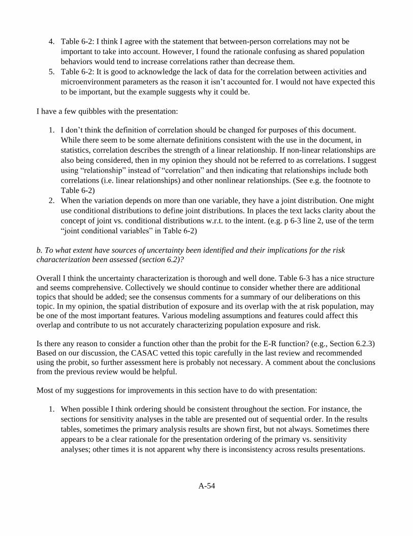
A-54

4. Table 6-2: I think I agree with the statement that between-person correlations may not be

important to take into account. However, I found the rationale confusing as shared population

behaviors would tend to increase correlations rather than decrease them.

5. Table 6-2: It is good to acknowledge the lack of data for the correlation between activities and

microenvironment parameters as the reason it isn’t accounted for. I would not have expected this

to be important, but the example suggests why it could be.

I have a few quibbles with the presentation:

1. I don’t think the definition of correlation should be changed for purposes of this document.

While there seem to be some alternate definitions consistent with the use in the document, in

statistics, correlation describes the strength of a linear relationship. If non-linear relationships are

also being considered, then in my opinion they should not be referred to as correlations. I suggest

using “relationship” instead of “correlation” and then indicating that relationships include both

correlations (i.e. linear relationships) and other nonlinear relationships. (See e.g. the footnote to

Table 6-2)

2. When the variation depends on more than one variable, they have a joint distribution. One might

use conditional distributions to define joint distributions. In places the text lacks clarity about the

concept of joint vs. conditional distributions w.r.t. to the intent. (e.g. p 6-3 line 2, use of the term

“joint conditional variables” in Table 6-2)



Overall I think the uncertainty characterization is thorough and well done. Table 6-3 has a nice structure

and seems comprehensive. Collectively we should continue to consider whether there are additional

topics that should be added; see the consensus comments for a summary of our deliberations on this

topic. In my opinion, the spatial distribution of exposure and its overlap with the at risk population, may

be one of the most important features. Various modeling assumptions and features could affect this

overlap and contribute to us not accurately characterizing population exposure and risk.

Is there any reason to consider a function other than the probit for the E-R function? (e.g., Section 6.2.3)

Based on our discussion, the CASAC vetted this topic carefully in the last review and recommended

using the probit, so further assessment here is probably not necessary. A comment about the conclusions

from the previous review would be helpful.

Most of my suggestions for improvements in this section have to do with presentation:

1. When possible I think ordering should be consistent throughout the section. For instance, the

sections for sensitivity analyses in the table are presented out of sequential order. In the results

tables, sometimes the primary analysis results are shown first, but not always. Sometimes there

appears to be a clear rationale for the presentation ordering of the primary vs. sensitivity

analyses; other times it is not apparent why there is inconsistency across results presentations.

A-55

2. I think every table (in e.g. a footnote) should make it clear which results are the primary analysis

and which are the sensitivity analysis. This will foster clarity and eliminate the need for readers

to look these up in other parts of the document.

3. Typically, the sensitivity analyses don’t show much impact. However, when there is an impact,

even a very small one, the direction of that impact is fairly consistently larger across conditions. I

think this should be stated directly and not left to the reader to ferret out. While I agree with the

general interpretations offered that the sensitivity results don’t alter the conclusions, I still think

the reporting should be more transparent about the fairly consistent direction of the very small

effects when they exist.

4. The comments in Table 6-3 should make it clear when they are describing sensitivity analysis

results. This isn’t immediately obvious for the estimation of continuous 5-minute concentrations

category.

5. Figures 6-1 to 6-3: Make sure to include the study area in the figure captions.

Other comments

P 4-25: Rounded down means truncated. Why not replace with truncated?

A-56

Dr. Frank Speizer

Chapter 3

Regarding the use of years 2011-2013, there is a remarkable decrease in exposure levels between 2011

and 2012-3. This is particularly true for Fall River. Is there something that happened between these

years to account for exposure differences? Alternatively, are we missing some data or did position of

monitors change for the later years. Since the focus in Chapter 5 is on Fall River, this should be detailed

here to avoid it coming as a question later.

Page 3-20, line 29: Simply for consistency sake should probably indicate the years for Indianapolis. (I

know it is described in next paragraph).

Chapter 4

Page 4-27, Figure 4-1. Although the data are presented in Table 4-10, the use of % response in both is

quite misleading. These are for most part frightfully small studies and as indicated in the table often the

positive responses are seen in 1 or two people. This is what it is but I wonder if it would be better to

characterize the findings “more qualitatively” in the Figures rather than relying on statistics.

Pages 4-27-4-30 sort of acts as a “teaser” for what to expect in Chapter 6. Not sure it could all have been

summed up by a single sentence (see chapter 6) but will have to wait until Chapter 6 is reviewed to see

just how redundant this is.

Chapter 5

The data and analyses discussed in this chapter is an excellent presentation of the 3 study areas

considered. The tables and figures really tell the story well and should set up for Chapter 6 details. I

congratulate staff for making this rather complex topic readable and informative. It appears to me to be

technically sound, and appropriately summarized and communicated, but I am still concerned as to the

direction of the exposure uncertainty created by the real differences between 2011 and the 2012-3 data.

Chapter 6

Page 6-5, table 6-1. In regard to the above, Microenvironmental spatial variability is mentioned as

potentially varying within and between study areas. This raises a red flag to me as a potential

explanation for the drastic variability between 2011 and 2012-3. A comment somewhere is needed.

Table 6-3 starting on page 6-8: Again, congrats to staff. I found this a most useful table to review in

detail. I have to admit I was looking for details that would explain the discrepancy between data for

2011 vs other years, but reading for details (which I did not find) was impressive that the potential

uncertainties have been characterized and considered.

A-57

Table B-1 Only suggestion so far that there was a difference in emissions in year 2011 vs other years

with a doubling of output. Not as true for other cities. (At least a potential explanation for differences in

exposure.

A-58

Dr. James Ultman

Chapter 5 – Exposure and Risk Assessment


Charge Question 9. This chapter is intended to be a concise summary of exposure and risk estimates, with

interpretation with regard to implications in this review largely being done in the PA. Does the Panel find

the information here to be technically sound, appropriately summarized and clearly communicated?

Within the many uncertainties in the risk analysis pointed out in Chapter 6, the general approach outlined in

this chapter is technically sound.

Clarity is somewhat lacking, however. This is understandable given the multiple data sources and complex

methodology that is used. Most troublesome to me was the lack of a clear definition of the subdivisions used

in the study areas: “AERMOD special grid” versus “receptors” vs “census blocks” versus “census blocks.”

Also of considerable importance throughout the document is “design value” which is never precisely defined

or explained.

There are three important shortcomings in the analysis. First, children (at exercise levels similar to those in

adult laboratory studies) are assigned the same exposure-response curve as that derived from adult laboratory

studies. I think that further elucidation of factors that may increase risk in children should be included (e.g.,

children have developing lungs so that long-term effects of SOx exposure may be important, even though

current research has not adequately addressed this). Second, the CHAD activity logs are not specific to

individuals with asthma. And asthmatics, particularly children, may spend less time outdoors than

nonasthmatics and exposure is greater outdoors than indoors. This factor leads to an overestimation of risk.

Third, the REA is limited to three study areas. There should be more discussion of how these results may be

viewed from a national public health perspective.

In figures 5-4 to 5-6, the overlay of DV and population density distributions, it is difficult to visually

separate the two variables. It might be better to make a 2-d plot of this type with a single combined

variable such as the product of DV with population density. In that case, the coincidence of large values

of the two variables would appear as the darkest pixels and the coincidence of small values would

appear as the lightest pixels.

On pg 4-26 and 4-27, more explanation of why probit function was selected for E-R functions.

Also, the text alludes to "two E-R" functions". It might clarify the discussion to refer to the two E-R

functions as E-R100 for a 100% decrement and E-R200 for a 200% decrement in sRaw. In figure 4-1, state

specifically what the bounding curves represent. Are they actually prediction intervals or are they

confidence limits? Were these bounds constructed as described on pg 6-35.

A-59

Dr. Ronald Wyzga

Overall Comments

The REA is an impressive and extensive document, the object of which is to estimate the potential risks

of short-term SO2 exposure to asthmatics. It concludes that the risks are very small to minimal at levels

of exposure which would be associated with current and other possible standards. The amount of work

carried out in this exercise is most impressive. Some changes or additions could be made to this work,

but it is questionable whether these changes would modify the overall conclusions. I cite at least 3 areas

where the analysis could have been altered/extended. In considering the prevalence of asthma in the

three study areas used as examples in this document, adjustment was made for several factors, but

apparently did not consider race, for which the prevalence varies. I don’t offhand know the racial

composition of the three areas studied, but unless they are radically different from the overall racial

distribution for the regions used to estimate prevalence, I suspect the overall results would change little.

It would be useful if the REA would briefly address this issue.

A second issue is the use of values for nearby geographic entities for the specific areas studies. I note,

for example, that air exchange rates for New York were used to estimate those for Fall River (and

Indianapolis, that also made use of data from Detroit) and those for Houston were used for Tulsa. While

specific data may not be available, use of data form other locations can create uncertainties in the

analyses that could impact results. For example, the housing stock in New York is very different from

that in Fall River. Air conditioning prevalence between Boston and Fall River could differ as well. This

uncertainty should be mentioned in the report, and its potential impact should be discussed.

The third issue is that the analysis considered the years 2011-2013. Several changes in emissions have

occurred since that period, resulting in even lower estimates of SO2 exposure. I note, for example, that

the Brayton Point power plant in Fall River was closed in July 2017, the PSO Northeastern Power

Station in Tulsa retired unit 4 in April 2016, the IPL- Harding Street Generating Station in Indianapolis

stopped burning coal in February 2016, and the Citizens Thermal unit in Indianapolis is presently

converting from coal to natural gas. All of these will significantly reduce SO2 emissions and lead to even

lower risk estimates. Although the analysis focused on the 2011-2013 time period for which extensive

data are available, these changes in emissions should at least be footnoted.

Charge question 10: What are the views of the Panel regarding the technical appropriateness of the

assessment of Uncertainty and variability, and the clarity in presentation?

a. To what extent has variability been described and appropriately represented (Section 6.1)?


characterization been assessed (Section 6.2)?

I am most concerned about any deviations from the assumed inputs into the model that would increase

the potential risks. Given the magnitude of estimated risks, factors that reduce the estimated low risks

are not of major interest in re-examining the SO2 NAAQS. I am less concerned about accuracy of

exposure/risk estimates than of potential underestimates.

There are, however, a couple of components in Table 6-1 that could be given more discussion: 1.)

Asthma prevalence - It is unclear to me why race was not considered in the estimates of asthma

A-60

prevalence. I doubt that introduction of this factor would lead to significant increases in the overall risk

estimates, but the potential omission of race as a predictor variable should be addressed in a brief

discussion. 2.) Microenvironmental approach - Limited available data made it necessary to utilize data

from other locations to estimate risks for the three study areas. It is unclear to me how differences

between the utilized data and the reality in the study communities would impact the results. I cite some

examples above. I know the Fall River area reasonably well; the housing stock there is very different

from that of New York; hence the estimates of air exchange rates for Fall River may be inaccurate. How

inaccurate need they be to substantially change the risk estimates. Similarly the removal rates are tied to

air conditioning prevalence. Boston data are used for Fall River. The difference in housing stock and

socio-economic factors between Boston and Fall River might influence the overall results. How

sensitive are the overall results to changes in these components?

Table 6-3 characterizes key uncertainties and tries to estimate their influence.

I have a few comments here:

Point Source Emissions and Profiles: Data from 2011 are used and are reasonably accurate; hence any

inaccuracies in the 2011 data are likely to be small and little impact on the exposure/risk estimates;

however there have several significant changes since 2011-13, and these would clearly impact the

exposure/risk estimates. This should be noted somewhere in the document, if only as a footnote.

APEX Microenvironmental Concentrations: See above comments. I wonder if the “low” Knowledge-

base uncertainty is correct for Indoor A/C Prevalence. This is also an element that is changing over time.

Specific Comments on document:

p. 3-9, Table 3-6: It should be clearly stated that these sources were for the period of study: 2011-2013.

A footnote might indicate known changes that have occurred since 2013.

p. 3-20, l. 29: To be consistent the years should be included here as well.

p. 4-4, ll. 4-5: I have seen state-specific data. Is there any reason why regional data were used rather than

state data?

ll. 10-18; Given the differences in prevalence among races, why is this not a consideration here?

P. 4-19, Table 4-7: Given the differences in housing stock and socio-economics between Boston and

Fall River, is there any need to consider these in the use of Boston data for Fall River?

B-1

Appendix B

Evaluation of SO2 Model Performance at Fall River, Indianapolis, and Tulsa

Prepared by: James Boylan

The first step in EPA’s Risk and Exposure Assessment was to model SO2 concentrations in three study

areas (Fall River, Indianapolis, and Tulsa) with AERMOD. AERMOD provides 1-hour SO2

concentrations that vary spatially and temporally. These modeling results are used to estimate 5-minute

SO2 exposures across the study areas and the risk assessment is built upon these results. If the

AERMOD model performance is significantly biased high or low, the resulting exposure assessment

will be significantly biased resulting in large uncertainties in the risk assessment. Therefore, it is critical

that the model has “acceptable” model performance. If the model does not have acceptable model

performance, the impacts of the model biases needs to be discussed and accounted for in the REA.

The final Integrated Science Assessment (ISA) states, “For models intended for application to

compliance assessments (e.g., related to the 1-h daily max SO2 standard), the model’s ability to capture

the high end of the concentration distribution is important. Measures such as robust highest

concentration (RHC) (Cox and Tikvart, 1990), and exploratory examinations of quantile-quantile plots

(Chambers et al., 1983) are useful. The RHC represents a smoothed estimate of the top values in the

distribution of hourly concentrations. In contrast, for dispersion modeling in support of health

studies where the model must capture concentrations at specified locations and time periods,

additional measures of bias and scatter are important.”

All three of the model evaluation methods used in Appendix D are associated with using the model for

regulatory compliance assessments. For example, the model’s ability to capture the high end of the

concentration distribution is evaluated with QQ-plots where the highest data point from the model is

compared to the highest data point from the observations even if they occur at a different time-of-day,

day-of-week, or season-of-year. In the REA, the model is being used to support health studies where

spatial and temporal accuracy is much more important compared with regulatory compliance

assessments. Since the Air Pollutants Exposure (APEX) model uses the model results paired in time and

space, the model results need to be evaluated against observations paired in time and space. Appendix

D does include absolute fractional bias (AFB) paired in space and presents QQ-plots paired in space

(Figures 1-3). However, there is no analysis or discussion on the model performance paired in space

and time.

During our September 18-19, 2017 meeting, the CASAC panel requested from EPA the 1-hour SO2

concentrations for 2011, 2012 and 2013 from each of the seven monitors included in Appendix D and

the modeled 1-hour SO2 concentrations from each receptor at the location of the monitor (paired in

time). On October 19, 2017 a memo from Erika Sasser (EPA) titled “CASAC Request for data

associated with Appendix D of the document titled Risk and Exposure Assessment for the Review of the

Primary National Ambient Air Quality Standard for Sulfur Oxides” was sent in response to the request.

In this memo, EPA states:

The AERMOD output for the three study areas was evaluated in Appendix D, consistent with

EPA’s model evaluation protocol that focuses on the higher concentrations in the concentration

distribution as those represent the concentrations of interest in regulatory applications. These

concentrations are also generally most important for the exposure assessment performed in the

B-2

draft REA. Given the uncertainty in emissions and meteorological inputs (e.g., wind direction) for

a given hour, EPA’s Guideline on Air Quality Models explicitly discourages pairing of model

estimates and monitor data on an hour-by-hour basis in evaluating performance of air quality

models. Appendix D recognized the uncertainties in available model inputs (i.e., emissions and

meteorology) for the three urban study areas, as well as the limited spatial coverage provided by

the seven monitors across the three study areas.

Given that the analyses in the draft REA involve a system of models, AERMOD model output

should be considered in terms of how it is being used in the Air Pollutants Exposure model

(APEX) to generate estimates of exposure as individuals move through time and space. In

particular, in evaluating model outputs, it is important to consider whether predicted high values

are occurring during times where people may be exercising in microenvironments where ambient

SO2 concentrations contribute to exposure. It is also appropriate to consider broad temporal

patterns in hourly concentrations (e.g., seasonal, weekday/weekend, times-of-day), which may be

more informative than comparing simultaneous hourly time-series of concentrations (e.g., model-

to-monitor comparisons).

The issue in the first paragraph is that EPA continues to rely on a model evaluation protocol that was

developed for regulatory applications which have a significantly different focus than health study

applications. EPA’s Guideline on Air Quality Models is appropriate for regulatory applications (PSD

permit modeling and SIP attainment demonstration modeling), but should not be applied to health study

applications (risk and exposure assessments) since the models are used in different ways. In the second

paragraph, EPA acknowledges the importance of timing of the high predicted values and states that it is

“appropriate to consider broad temporal patterns in hourly concentrations (e.g., seasonal,

weekday/weekend, times-of-day)”. I would agree with EPA that broad temporal patterns in hourly

concentrations (e.g., time-of-day, day-of-week (weekday/weekend), or season-of-year) are more

informative than comparing simultaneous hourly time-series of concentrations because exposures during

identical times-of-day, days-of-week (weekday/weekend), and seasons-of- year are treated the same by

the APEX model. However, EPA has made no effort to look at whether predicted high values are

occurring at the right time-of-day, day-of-week, or season-of-year.

To address this shortcoming, I performed a model performance evaluation comparing 1-hour SO2 model

concentrations against measurements at one monitor in Fall River, MA (250051004); three monitors in

Indianapolis, IN (180970057, 180970073, and 180970078); and three monitors in Tulsa, OK

(401430175, 401430235, and 401431127). The 1-hour SO2 model concentrations and measurements

were provided by EPA. Since there are very few SO2 monitors in the study areas, it can be assumed that

good performance at the monitoring sites indicates good model performance at the receptors that don’t

have monitors. Conversely, poor performance at the monitoring sites indicates poor model performance

at the receptors that don’t have monitors.

To prepare the data for analysis, I removed all data pairs with an invalid measurement value (-999)

and/or an invalid modeling value (-999). AERMOD can’t calculate a concentration when the wind

speed is zero, resulting in a null value (-999). Then, a number of model evaluations were performed to

better understand the model performance paired in time and space. After looking at the results, it was

determined that the most informative graphical depictions were maximum modeled 1-hour SO2

concentration vs. maximum measured 1-hour SO2 concentration by hour-of-day for each monitor site,

where the maximum values were obtained for each hour across the three year period that was evaluated

(2011-2013). In addition, QQ-plots for each hour-of-day provide additional details for the rest of the

distribution. Since time-of-day is an important variable in the APEX model, QQ-plots for each hour-of-

B-3

day is much more appropriate than QQ-plots that are unpaired in time. Also, the higher concentrations

in the distribution are generally more important for the exposure assessment in the REA; therefore,

performance of those values should be given more weight than lower concentrations. Since it is not

likely that any modeled or measured 1-hour SO2 concentrations less than 50 ppb will result in a 5-

minute SO2 concentration above 200 ppb, most of the analysis will focus on the modeled and measured

1-hour SO2 concentrations above 50 ppb. The approach described above is a simple approach and does

not account for differences in day-of-week or season-of-year. Therefore, the summary of results

presented below can be considered the best case scenario since accounting for day-of-week and season-

of-year in addition to time-of-day would show larger biases between measured and monitored SO2

concentrations. A summary of the MPE results for each monitor location are presented below.

Fall River, MA (250051004)

See Figure 4 and Figures 11-16. For Hours 1-6 and 19-24, the 1-hour SO2 observations are ~4x higher

than the modeled values. Smaller biases (both positive and negative) are seen in Hours 7-18, with a few

outliers in Hours 9, 10, 11, and 13.

Indianapolis, IN (180970057)

See Figure 5 and Figures 17-22. For Hours 1-7 and 18-24, the 1-hour SO2 modeled values are ~2x

higher than the observations. Smaller biases (both positive and negative) are seen in Hours 8-17, with a

few outliers in Hours 10, 11, and 12.


See Figure 6 and Figures 23-28. For Hours 1-8 and 18-24, all modeled and measured 1-hour SO2

concentrations are below 52 ppb and the model bias is small. For Hours 9-17, the 1-hour SO2

observations are ~2-3x higher than the modeled values.


See Figure 7 and Figures 29-34. For Hours 1-8 and 16-24, all modeled and measured 1-hour SO2

concentrations are below 64 ppb and the model bias is small. For Hours 9-15, the 1-hour SO2

observations are ~2x higher than the modeled values.

Tulsa, OK (401430175)

See Figure 8 and Figures 35-40. For Hours 1-9 and 20-24, the model bias is small. For Hours 10-19,

the 1-hour SO2 observations are ~2-3x higher than the modeled values.

Tulsa, OK (401430235)

See Figure 9 and Figures 41-46. All modeled and measured 1-hour SO2 concentrations are below 50

ppb, except for Hours 1 and 24 where the maximum 1-hour SO2 observations are 64 ppb and 53 ppb.

For Hours 1-8 and 17-24, the 1-hour SO2 modeled values are ~1.5-2x higher than the observations.

Smaller biases (both positive and negative) are seen in Hours 9-16, with a few outliers in Hours 10 and

11.

Tulsa, OK (401431127)

See Figure 10 and Figures 47-52. All modeled and measured 1-hour SO2 concentrations are below 40

ppb. For Hours 1-8 and 17-24, the 1-hour SO2 modeled values are ~1.5-2x higher than the observations,

except for observations above 20 ppb which match well with the modeled values. Smaller biases (both

positive and negative) are seen in Hours 9-16, except for the observations above 20 ppb which the model

underestimates by a factor of 1.5-2x.

B-4

Conclusion

The model performance varies by monitoring site and time-of-day. For Fall River (250051004), the

early morning and late evening 1-hour SO2 observations are ~4x higher than the modeled values. For

one Indianapolis monitor (180970057), the early morning and late evening 1-hour SO2 modeled values

are ~2x higher than the observations. For the other two Indianapolis monitors (180970073 and

180970078), the late morning, afternoon, and early evening 1-hour SO2 observations are ~2-3x higher

than the modeled values. For one Tulsa monitor (401430175), the late morning, afternoon, and early

evening 1-hour SO2 observations are ~2-3x higher than the modeled values. For the other two Tulsa

monitors (401430235 and 401431127), early morning and late evening 1-hour SO2 modeled values are

~1.5-2x higher than the observations. These model biases will have a direct impact on the APEX

results, possibly calling into question the percent of children and adults experiencing 5-minute exposures

at or above 200 ppb. In addition, EPA should examine the day-of-week (weekday/weekend) and

season-of-year model performance. Finally, the time-of-day, day-of-week (weekday/weekend), and

season-of-year model biases should be discussed and accounted for in the final REA.

B-5

Figure 1. 1-hour SO2 QQ plots (g/m3) for Fall River, MA (unpaired in time) from EPA’s REA

(Figure D-1).

B-6

Figure 2. 1-hour SO2 QQ plots (g/m3) for individual monitors in Indianapolis, IN (unpaired in time) from EPA’s REA (Figure D-7).

B-7

Figure 3. 1-hour SO2 QQ plots (g/m3) for individual monitors in Tulsa, OK (unpaired in time) from EPA’s REA (Figure D-13).

B-8

Figure 4. Maximum modeled 1-hour SO2 concentration vs. maximum measured 1-hour SO2

concentration by hour-of-day for Fall River, MA (250051004).


concentration by hour-of-day for Indianapolis, IN (180970057).

0.0

20.0

40.0

60.0

80.0

100.0

120.0

140.0

160.0

1 2 3 4 5 6 7 8 9 10 11 12 13 14 15 16 17 18 19 20 21 22 23 24

SO2

Co

nce

ntr

atio

n (

pp

b)

Maximum Values at 250051004

Max of AERMOD (ppb) Max of Obs (ppb)

0.0

50.0

100.0

150.0

200.0

250.0

1 2 3 4 5 6 7 8 9 10 11 12 13 14 15 16 17 18 19 20 21 22 23 24

SO2

Co

nce

ntr

atio

n (

pp

b)



B-9





0.0

50.0

100.0

150.0

200.0

250.0

1 2 3 4 5 6 7 8 9 10 11 12 13 14 15 16 17 18 19 20 21 22 23 24

SO2

Co

nce

ntr

atio

n (

pp

b)



0.0

20.0

40.0

60.0

80.0

100.0

120.0

1 2 3 4 5 6 7 8 9 10 11 12 13 14 15 16 17 18 19 20 21 22 23 24

SO2

Co

nce

ntr

atio

n (

pp

b)



B-10


concentration by hour-of-day for Tulsa, OK (401430175).



0.0

10.0

20.0

30.0

40.0

50.0

60.0

70.0

80.0

90.0

1 2 3 4 5 6 7 8 9 10 11 12 13 14 15 16 17 18 19 20 21 22 23 24

SO2

Co

nce

ntr

atio

n (

pp

b)



0.0

10.0

20.0

30.0

40.0

50.0

60.0

70.0

1 2 3 4 5 6 7 8 9 10 11 12 13 14 15 16 17 18 19 20 21 22 23 24

SO2

Co

nce

ntr

atio

n (

pp

b)



B-11



0.0

5.0

10.0

15.0

20.0

25.0

30.0

35.0

40.0

1 2 3 4 5 6 7 8 9 10 11 12 13 14 15 16 17 18 19 20 21 22 23 24

SO2

Co

nce

ntr

atio

n (

pp

b)



B-12

Figure 11. QQ-plots for measured 1-hour SO2 concentration vs. modeled 1-hour SO2 concentration by hour-of-day for Fall River, MA (250051004).

0

20

40

60

80

100

0 20 40 60 80 100

AER

MO

D (

pp

b)

Observations (ppb)

SO2 at 250051004 - Hour 1

0

20

40

60

80

100

0 20 40 60 80 100

AER

MO

D(p

pb

)

Observations (ppb)

SO2 at 250051004 - Hour 2

0

20

40

60

80

100

0 20 40 60 80 100

AER

MO

D(p

pb

)

Observations (ppb)

SO2 at 250051004 - Hour 3

0

20

40

60

80

100

0 20 40 60 80 100

AER

MO

D(p

pb

)

Observations (ppb)

SO2 at 250051004 - Hour 4

B-13


0

20

40

60

80

100

0 20 40 60 80 100

AER

MO

D(p

pb

)

Observations (ppb)

SO2 at 250051004 - Hour 5

0

20

40

60

80

100

0 20 40 60 80 100

AER

MO

D(p

pb

)

Observations (ppb)

SO2 at 250051004 - Hour 6

0

20

40

60

80

100

120

0 20 40 60 80 100 120

AER

MO

D(p

pb

)

Observations (ppb)

SO2 at 250051004 - Hour 7

0

20

40

60

80

100

120

140

0 20 40 60 80 100 120 140

AER

MO

D(p

pb

)

Observations (ppb)

SO2 at 250051004 - Hour 8

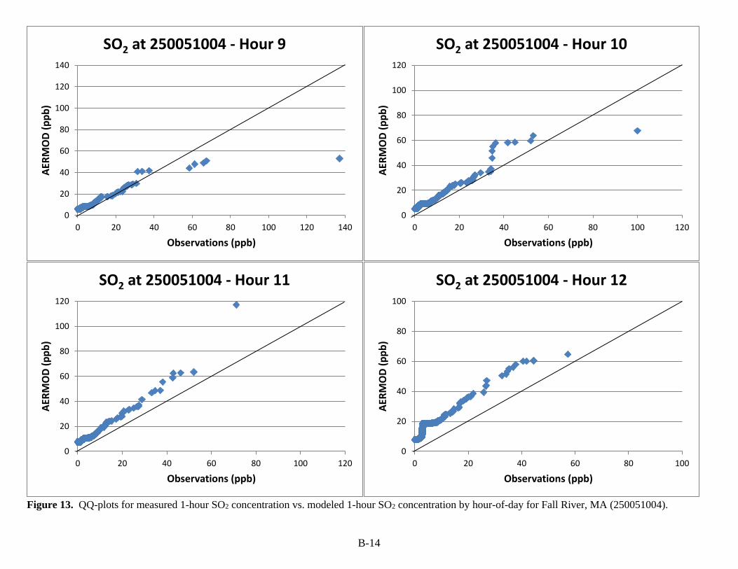
B-14


0

20

40

60

80

100

120

140

0 20 40 60 80 100 120 140

AER

MO

D(p

pb

)

Observations (ppb)

SO2 at 250051004 - Hour 9

0

20

40

60

80

100

120

0 20 40 60 80 100 120

AER

MO

D(p

pb

)

Observations (ppb)

SO2 at 250051004 - Hour 10

0

20

40

60

80

100

120

0 20 40 60 80 100 120

AER

MO

D(p

pb

)

Observations (ppb)

SO2 at 250051004 - Hour 11

0

20

40

60

80

100

0 20 40 60 80 100

AER

MO

D(p

pb

)

Observations (ppb)

SO2 at 250051004 - Hour 12

B-15


0

20

40

60

80

100

120

140

0 20 40 60 80 100 120 140

AER

MO

D (

pp

b)

Observations (ppb)

SO2 at 250051004 - Hour 13

0

20

40

60

80

100

0 20 40 60 80 100

AER

MO

D (

pp

b)

Observations (ppb)

SO2 at 250051004 - Hour 14

0

20

40

60

80

100

0 20 40 60 80 100

AER

MO

D (

pp

b)

Observations (ppb)

SO2 at 250051004 - Hour 15

0

20

40

60

80

100

0 20 40 60 80 100

AER

MO

D (

pp

b)

Observations (ppb)

SO2 at 250051004 - Hour 16

B-16


0

20

40

60

80

100

0 20 40 60 80 100

AER

MO

D (

pp

b)

Observations (ppb)

SO2 at 250051004 - Hour 17

0

20

40

60

80

100

0 20 40 60 80 100

AER

MO

D (

pp

b)

Observations (ppb)

SO2 at 250051004 - Hour 18

0

20

40

60

80

100

0 20 40 60 80 100

AER

MO

D (

pp

b)

Observations (ppb)

SO2 at 250051004 - Hour 19

0

20

40

60

80

100

0 20 40 60 80 100

AER

MO

D (

pp

b)

Observations (ppb)

SO2 at 250051004 - Hour 20

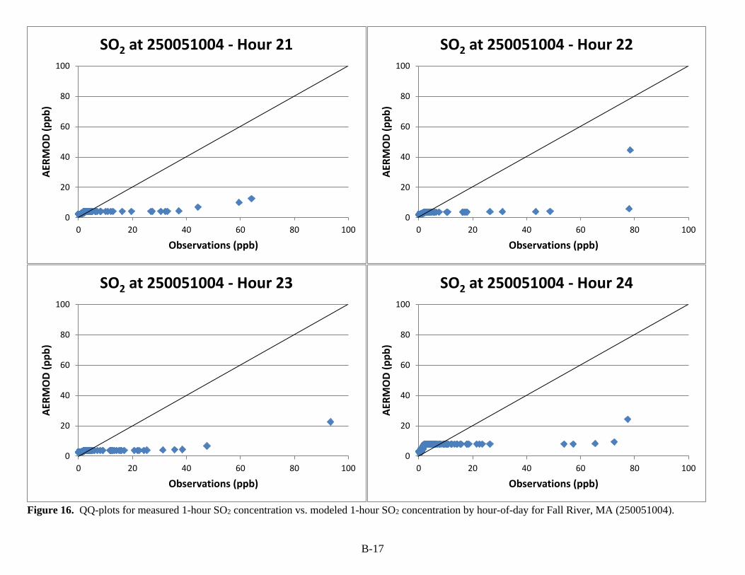
B-17


0

20

40

60

80

100

0 20 40 60 80 100

AER

MO

D (

pp

b)

Observations (ppb)

SO2 at 250051004 - Hour 21

0

20

40

60

80

100

0 20 40 60 80 100

AER

MO

D (

pp

b)

Observations (ppb)

SO2 at 250051004 - Hour 22

0

20

40

60

80

100

0 20 40 60 80 100

AER

MO

D (

pp

b)

Observations (ppb)

SO2 at 250051004 - Hour 23

0

20

40

60

80

100

0 20 40 60 80 100

AER

MO

D (

pp

b)

Observations (ppb)

SO2 at 250051004 - Hour 24

B-18

Figure 17. QQ-plots for measured 1-hour SO2 concentration vs. modeled 1-hour SO2 concentration by hour-of-day for Indianapolis, IN (180970057).

0

20

40

60

80

100

120

140

0 20 40 60 80 100 120 140

AER

MO

D (

pp

b)

Observations (ppb)

SO2 at 180970057 - Hour 1

0

20

40

60

80

100

120

140

0 20 40 60 80 100 120 140

AER

MO

D(p

pb

)

Observations (ppb)

SO2 at 180970057 - Hour 2

0

20

40

60

80

100

120

140

0 20 40 60 80 100 120 140

AER

MO

D(p

pb

)

Observations (ppb)

SO2 at 180970057 - Hour 3

0

20

40

60

80

100

120

0 20 40 60 80 100 120

AER

MO

D(p

pb

)

Observations (ppb)

SO2 at 180970057 - Hour 4

B-19


0

20

40

60

80

100

120

0 20 40 60 80 100 120

AER

MO

D(p

pb

)

Observations (ppb)

SO2 at 180970057 - Hour 5

0

20

40

60

80

100

0 20 40 60 80 100

AER

MO

D(p

pb

)

Observations (ppb)

SO2 at 180970057 - Hour 6

0

20

40

60

80

100

120

0 20 40 60 80 100 120

AER

MO

D(p

pb

)

Observations (ppb)

SO2 at 180970057 - Hour 7

0

20

40

60

80

100

120

0 20 40 60 80 100 120

AER

MO

D(p

pb

)

Observations (ppb)

SO2 at 180970057 - Hour 8

B-20


0

20

40

60

80

100

120

0 20 40 60 80 100 120

AER

MO

D(p

pb

)

Observations (ppb)

SO2 at 180970057 - Hour 9

0

20

40

60

80

100

120

140

160

180

0 20 40 60 80 100 120 140 160 180

AER

MO

D(p

pb

)

Observations (ppb)

SO2 at 180970057 - Hour 10

0

20

40

60

80

100

120

140

160

180

200

220

0 20 40 60 80 100 120 140 160 180 200 220

AER

MO

D(p

pb

)

Observations (ppb)

SO2 at 180970057 - Hour 11

0

20

40

60

80

100

120

140

160

0 20 40 60 80 100 120 140 160

AER

MO

D(p

pb

)

Observations (ppb)

SO2 at 180970057 - Hour 12

B-21


0

20

40

60

80

100

120

0 20 40 60 80 100 120

AER

MO

D (

pp

b)

Observations (ppb)

SO2 at 180970057 - Hour 13

0

20

40

60

80

100

120

0 20 40 60 80 100 120

AER

MO

D (

pp

b)

Observations (ppb)

SO2 at 180970057 - Hour 14

0

20

40

60

80

100

120

0 20 40 60 80 100 120

AER

MO

D (

pp

b)

Observations (ppb)

SO2 at 180970057 - Hour 15

0

20

40

60

80

100

120

0 20 40 60 80 100 120

AER

MO

D (

pp

b)

Observations (ppb)

SO2 at 180970057 - Hour 16

B-22


0

20

40

60

80

100

0 20 40 60 80 100

AER

MO

D (

pp

b)

Observations (ppb)

SO2 at 180970057 - Hour 17

0

20

40

60

80

100

120

140

0 20 40 60 80 100 120 140

AER

MO

D (

pp

b)

Observations (ppb)

SO2 at 180970057 - Hour 18

0

20

40

60

80

100

120

140

160

180

0 20 40 60 80 100 120 140 160 180

AER

MO

D (

pp

b)

Observations (ppb)

SO2 at 180970057 - Hour 19

0

20

40

60

80

100

120

0 20 40 60 80 100 120

AER

MO

D (

pp

b)

Observations (ppb)

SO2 at 180970057 - Hour 20

B-23


0

20

40

60

80

100

120

140

0 20 40 60 80 100 120 140

AER

MO

D (

pp

b)

Observations (ppb)

SO2 at 180970057 - Hour 21

0

20

40

60

80

100

120

140

160

0 20 40 60 80 100 120 140 160

AER

MO

D (

pp

b)

Observations (ppb)

SO2 at 180970057 - Hour 22

0

20

40

60

80

100

120

0 20 40 60 80 100 120

AER

MO

D (

pp

b)

Observations (ppb)

SO2 at 180970057 - Hour 23

0

20

40

60

80

100

120

140

0 20 40 60 80 100 120 140

AER

MO

D (

pp

b)

Observations (ppb)

SO2 at 180970057 - Hour 24

B-24


0

20

40

60

80

100

0 20 40 60 80 100

AER

MO

D (

pp

b)

Observations (ppb)

SO2 at 180970073 - Hour 1

0

20

40

60

80

100

0 20 40 60 80 100

AER

MO

D(p

pb

)

Observations (ppb)

SO2 at 180970073 - Hour 2

0

20

40

60

80

100

0 20 40 60 80 100

AER

MO

D(p

pb

)

Observations (ppb)

SO2 at 180970073 - Hour 3

0

20

40

60

80

100

0 20 40 60 80 100

AER

MO

D(p

pb

)

Observations (ppb)

SO2 at 180970073 - Hour 4

B-25


0

20

40

60

80

100

0 20 40 60 80 100

AER

MO

D(p

pb

)

Observations (ppb)

SO2 at 180970073 - Hour 5

0

20

40

60

80

100

0 20 40 60 80 100

AER

MO

D(p

pb

)

Observations (ppb)

SO2 at 180970073 - Hour 6

0

20

40

60

80

100

0 20 40 60 80 100

AER

MO

D(p

pb

)

Observations (ppb)

SO2 at 180970073 - Hour 7

0

20

40

60

80

100

0 20 40 60 80 100

AER

MO

D(p

pb

)

Observations (ppb)

SO2 at 180970073 - Hour 8

B-26


0

20

40

60

80

100

120

140

160

180

200

220

0 20 40 60 80 100 120 140 160 180 200 220

AER

MO

D(p

pb

)

Observations (ppb)

SO2 at 180970073 - Hour 9

0

20

40

60

80

100

0 20 40 60 80 100

AER

MO

D(p

pb

)

Observations (ppb)

SO2 at 180970073 - Hour 10

0

20

40

60

80

100

0 20 40 60 80 100

AER

MO

D(p

pb

)

Observations (ppb)

SO2 at 180970073 - Hour 11

0

20

40

60

80

100

0 20 40 60 80 100

AER

MO

D(p

pb

)

Observations (ppb)

SO2 at 180970073 - Hour 12

B-27


0

20

40

60

80

100

0 20 40 60 80 100

AER

MO

D (

pp

b)

Observations (ppb)

SO2 at 180970073 - Hour 13

0

20

40

60

80

100

0 20 40 60 80 100

AER

MO

D (

pp

b)

Observations (ppb)

SO2 at 180970073 - Hour 14

0

20

40

60

80

100

0 20 40 60 80 100

AER

MO

D (

pp

b)

Observations (ppb)

SO2 at 180970073 - Hour 15

0

20

40

60

80

100

120

0 20 40 60 80 100 120

AER

MO

D (

pp

b)

Observations (ppb)

SO2 at 180970073 - Hour 16

B-28


0

20

40

60

80

100

0 20 40 60 80 100

AER

MO

D (

pp

b)

Observations (ppb)

SO2 at 180970073 - Hour 17

0

20

40

60

80

100

0 20 40 60 80 100

AER

MO

D (

pp

b)

Observations (ppb)

SO2 at 180970073 - Hour 18

0

20

40

60

80

100

0 20 40 60 80 100

AER

MO

D (

pp

b)

Observations (ppb)

SO2 at 180970073 - Hour 19

0

20

40

60

80

100

0 20 40 60 80 100

AER

MO

D (

pp

b)

Observations (ppb)

SO2 at 180970073 - Hour 20

B-29


0

20

40

60

80

100

0 20 40 60 80 100

AER

MO

D (

pp

b)

Observations (ppb)

SO2 at 180970073 - Hour 21

0

20

40

60

80

100

0 20 40 60 80 100

AER

MO

D (

pp

b)

Observations (ppb)

SO2 at 180970073 - Hour 22

0

20

40

60

80

100

0 20 40 60 80 100

AER

MO

D (

pp

b)

Observations (ppb)

SO2 at 180970073 - Hour 23

0

20

40

60

80

100

0 20 40 60 80 100

AER

MO

D (

pp

b)

Observations (ppb)

SO2 at 180970073 - Hour 24

B-30


0

20

40

60

80

100

0 20 40 60 80 100

AER

MO

D (

pp

b)

Observations (ppb)

SO2 at 180970078 - Hour 1

0

20

40

60

80

100

0 20 40 60 80 100

AER

MO

D(p

pb

)

Observations (ppb)

SO2 at 180970078 - Hour 2

0

20

40

60

80

100

0 20 40 60 80 100

AER

MO

D(p

pb

)

Observations (ppb)

SO2 at 180970078 - Hour 3

0

20

40

60

80

100

0 20 40 60 80 100

AER

MO

D(p

pb

)

Observations (ppb)

SO2 at 180970078 - Hour 4

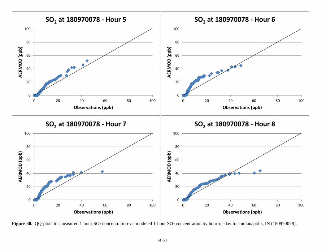
B-31


0

20

40

60

80

100

0 20 40 60 80 100

AER

MO

D(p

pb

)

Observations (ppb)

SO2 at 180970078 - Hour 5

0

20

40

60

80

100

0 20 40 60 80 100

AER

MO

D(p

pb

)

Observations (ppb)

SO2 at 180970078 - Hour 6

0

20

40

60

80

100

0 20 40 60 80 100

AER

MO

D(p

pb

)

Observations (ppb)

SO2 at 180970078 - Hour 7

0

20

40

60

80

100

0 20 40 60 80 100

AER

MO

D(p

pb

)

Observations (ppb)

SO2 at 180970078 - Hour 8

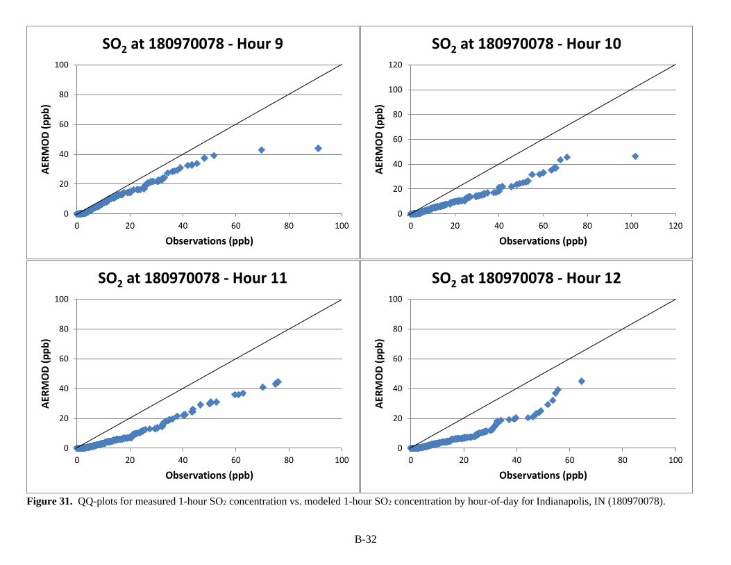
B-32


0

20

40

60

80

100

0 20 40 60 80 100

AER

MO

D(p

pb

)

Observations (ppb)

SO2 at 180970078 - Hour 9

0

20

40

60

80

100

120

0 20 40 60 80 100 120

AER

MO

D(p

pb

)

Observations (ppb)

SO2 at 180970078 - Hour 10

0

20

40

60

80

100

0 20 40 60 80 100

AER

MO

D(p

pb

)

Observations (ppb)

SO2 at 180970078 - Hour 11

0

20

40

60

80

100

0 20 40 60 80 100

AER

MO

D(p

pb

)

Observations (ppb)

SO2 at 180970078 - Hour 12

B-33


0

20

40

60

80

100

0 20 40 60 80 100

AER

MO

D (

pp

b)

Observations (ppb)

SO2 at 180970078 - Hour 13

0

20

40

60

80

100

0 20 40 60 80 100

AER

MO

D (

pp

b)

Observations (ppb)

SO2 at 180970078 - Hour 14

0

20

40

60

80

100

0 20 40 60 80 100

AER

MO

D (

pp

b)

Observations (ppb)

SO2 at 180970078 - Hour 15

0

20

40

60

80

100

0 20 40 60 80 100

AER

MO

D (

pp

b)

Observations (ppb)

SO2 at 180970078 - Hour 16

B-34


0

20

40

60

80

100

0 20 40 60 80 100

AER

MO

D (

pp

b)

Observations (ppb)

SO2 at 180970078 - Hour 17

0

20

40

60

80

100

0 20 40 60 80 100

AER

MO

D (

pp

b)

Observations (ppb)

SO2 at 180970078 - Hour 18

0

20

40

60

80

100

0 20 40 60 80 100

AER

MO

D (

pp

b)

Observations (ppb)

SO2 at 180970078 - Hour 19

0

20

40

60

80

100

0 20 40 60 80 100

AER

MO

D (

pp

b)

Observations (ppb)

SO2 at 180970078 - Hour 20

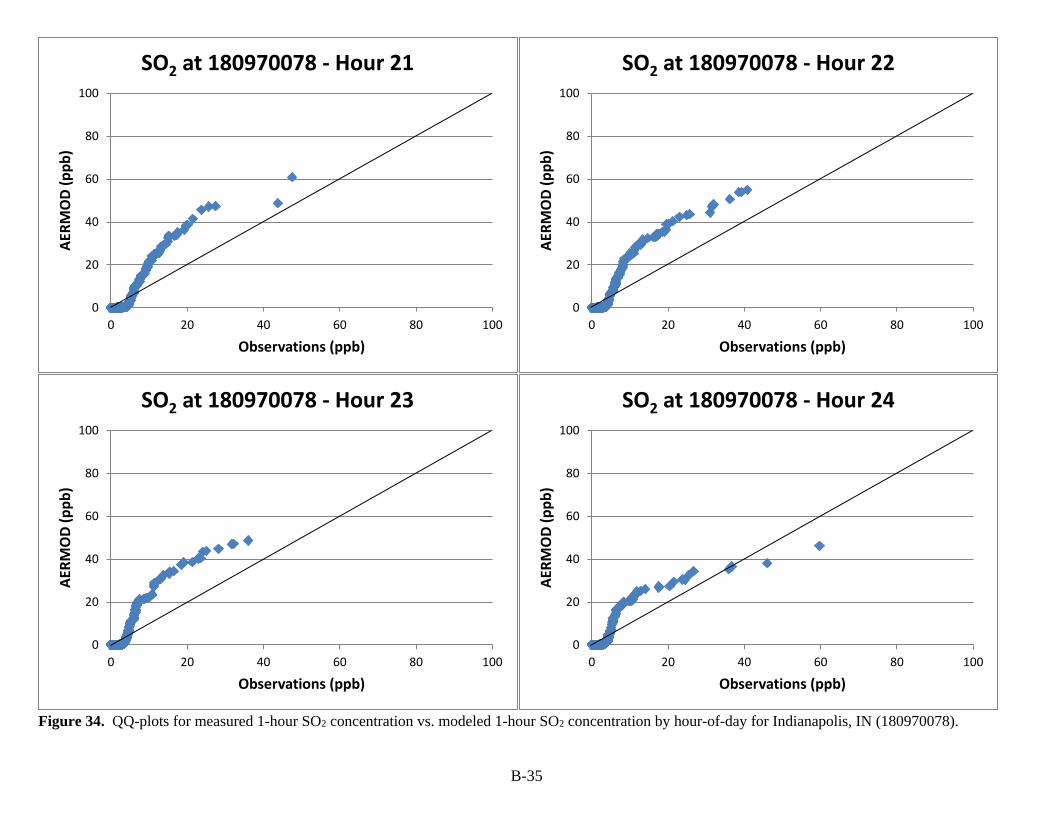
B-35


0

20

40

60

80

100

0 20 40 60 80 100

AER

MO

D (

pp

b)

Observations (ppb)

SO2 at 180970078 - Hour 21

0

20

40

60

80

100

0 20 40 60 80 100

AER

MO

D (

pp

b)

Observations (ppb)

SO2 at 180970078 - Hour 22

0

20

40

60

80

100

0 20 40 60 80 100

AER

MO

D (

pp

b)

Observations (ppb)

SO2 at 180970078 - Hour 23

0

20

40

60

80

100

0 20 40 60 80 100

AER

MO

D (

pp

b)

Observations (ppb)

SO2 at 180970078 - Hour 24

B-36

Figure 35. QQ-plots for measured 1-hour SO2 concentration vs. modeled 1-hour SO2 concentration by hour-of-day for Tulsa, OK (401430175).

0

20

40

60

80

100

0 20 40 60 80 100

AER

MO

D (

pp

b)

Observations (ppb)

SO2 at 401430175 - Hour 1

0

20

40

60

80

100

0 20 40 60 80 100

AER

MO

D(p

pb

)

Observations (ppb)

SO2 at 401430175 - Hour 2

0

20

40

60

80

100

0 20 40 60 80 100

AER

MO

D(p

pb

)

Observations (ppb)

SO2 at 401430175 - Hour 3

0

20

40

60

80

100

0 20 40 60 80 100

AER

MO

D(p

pb

)

Observations (ppb)

SO2 at 401430175 - Hour 4

B-37


0

20

40

60

80

100

0 20 40 60 80 100

AER

MO

D(p

pb

)

Observations (ppb)

SO2 at 401430175 - Hour 5

0

20

40

60

80

100

0 20 40 60 80 100

AER

MO

D(p

pb

)

Observations (ppb)

SO2 at 401430175 - Hour 6

0

20

40

60

80

100

0 20 40 60 80 100

AER

MO

D(p

pb

)

Observations (ppb)

SO2 at 401430175 - Hour 7

0

20

40

60

80

100

0 20 40 60 80 100

AER

MO

D(p

pb

)

Observations (ppb)

SO2 at 401430175 - Hour 8

B-38


0

20

40

60

80

100

0 20 40 60 80 100

AER

MO

D(p

pb

)

Observations (ppb)

SO2 at 401430175 - Hour 9

0

20

40

60

80

100

0 20 40 60 80 100

AER

MO

D(p

pb

)

Observations (ppb)

SO2 at 401430175 - Hour 10

0

20

40

60

80

100

0 20 40 60 80 100

AER

MO

D(p

pb

)

Observations (ppb)

SO2 at 401430175 - Hour 11

0

20

40

60

80

100

0 20 40 60 80 100

AER

MO

D(p

pb

)

Observations (ppb)

SO2 at 401430175 - Hour 12

B-39


0

20

40

60

80

100

0 20 40 60 80 100

AER

MO

D (

pp

b)

Observations (ppb)

SO2 at 401430175 - Hour 13

0

20

40

60

80

100

0 20 40 60 80 100

AER

MO

D (

pp

b)

Observations (ppb)

SO2 at 401430175 - Hour 14

0

20

40

60

80

100

0 20 40 60 80 100

AER

MO

D (

pp

b)

Observations (ppb)

SO2 at 401430175 - Hour 15

0

20

40

60

80

100

0 20 40 60 80 100

AER

MO

D (

pp

b)

Observations (ppb)

SO2 at 401430175 - Hour 16

B-40


0

20

40

60

80

100

0 20 40 60 80 100

AER

MO

D (

pp

b)

Observations (ppb)

SO2 at 401430175 - Hour 17

0

20

40

60

80

100

0 20 40 60 80 100

AER

MO

D (

pp

b)

Observations (ppb)

SO2 at 401430175 - Hour 18

0

20

40

60

80

100

0 20 40 60 80 100

AER

MO

D (

pp

b)

Observations (ppb)

SO2 at 401430175 - Hour 19

0

20

40

60

80

100

0 20 40 60 80 100

AER

MO

D (

pp

b)

Observations (ppb)

SO2 at 401430175 - Hour 20

B-41


0

20

40

60

80

100

0 20 40 60 80 100

AER

MO

D (

pp

b)

Observations (ppb)

SO2 at 401430175 - Hour 21

0

20

40

60

80

100

0 20 40 60 80 100

AER

MO

D (

pp

b)

Observations (ppb)

SO2 at 401430175 - Hour 22

0

20

40

60

80

100

0 20 40 60 80 100

AER

MO

D (

pp

b)

Observations (ppb)

SO2 at 401430175 - Hour 23

0

20

40

60

80

100

0 20 40 60 80 100

AER

MO

D (

pp

b)

Observations (ppb)

SO2 at 401430175 - Hour 24

B-42


0

20

40

60

80

100

0 20 40 60 80 100

AER

MO

D (

pp

b)

Observations (ppb)

SO2 at 401430235 - Hour 1

0

20

40

60

80

100

0 20 40 60 80 100

AER

MO

D(p

pb

)

Observations (ppb)

SO2 at 401430235 - Hour 2

0

20

40

60

80

100

0 20 40 60 80 100

AER

MO

D(p

pb

)

Observations (ppb)

SO2 at 401430235 - Hour 3

0

20

40

60

80

100

0 20 40 60 80 100

AER

MO

D(p

pb

)

Observations (ppb)

SO2 at 401430235 - Hour 4

B-43


0

20

40

60

80

100

0 20 40 60 80 100

AER

MO

D(p

pb

)

Observations (ppb)

SO2 at 401430235 - Hour 5

0

20

40

60

80

100

0 20 40 60 80 100

AER

MO

D(p

pb

)

Observations (ppb)

SO2 at 401430235 - Hour 6

0

20

40

60

80

100

0 20 40 60 80 100

AER

MO

D(p

pb

)

Observations (ppb)

SO2 at 401430235 - Hour 7

0

20

40

60

80

100

0 20 40 60 80 100

AER

MO

D(p

pb

)

Observations (ppb)

SO2 at 401430235 - Hour 8

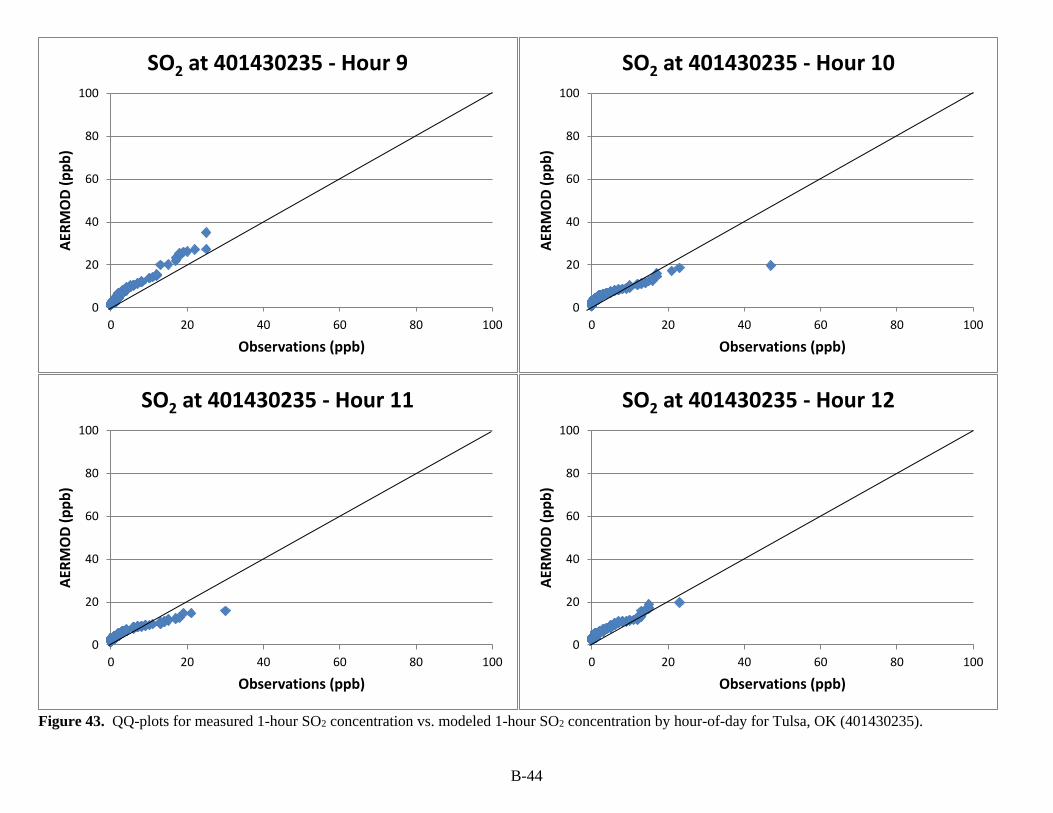
B-44


0

20

40

60

80

100

0 20 40 60 80 100

AER

MO

D(p

pb

)

Observations (ppb)

SO2 at 401430235 - Hour 9

0

20

40

60

80

100

0 20 40 60 80 100

AER

MO

D(p

pb

)

Observations (ppb)

SO2 at 401430235 - Hour 10

0

20

40

60

80

100

0 20 40 60 80 100

AER

MO

D(p

pb

)

Observations (ppb)

SO2 at 401430235 - Hour 11

0

20

40

60

80

100

0 20 40 60 80 100

AER

MO

D(p

pb

)

Observations (ppb)

SO2 at 401430235 - Hour 12

B-45


0

20

40

60

80

100

0 20 40 60 80 100

AER

MO

D (

pp

b)

Observations (ppb)

SO2 at 401430235 - Hour 13

0

20

40

60

80

100

0 20 40 60 80 100

AER

MO

D (

pp

b)

Observations (ppb)

SO2 at 401430235 - Hour 14

0

20

40

60

80

100

0 20 40 60 80 100

AER

MO

D (

pp

b)

Observations (ppb)

SO2 at 401430235 - Hour 15

0

20

40

60

80

100

0 20 40 60 80 100

AER

MO

D (

pp

b)

Observations (ppb)

SO2 at 401430235 - Hour 16

B-46


0

20

40

60

80

100

0 20 40 60 80 100

AER

MO

D (

pp

b)

Observations (ppb)

SO2 at 401430235 - Hour 17

0

20

40

60

80

100

0 20 40 60 80 100

AER

MO

D (

pp

b)

Observations (ppb)

SO2 at 401430235 - Hour 18

0

20

40

60

80

100

0 20 40 60 80 100

AER

MO

D (

pp

b)

Observations (ppb)

SO2 at 401430235 - Hour 19

0

20

40

60

80

100

0 20 40 60 80 100

AER

MO

D (

pp

b)

Observations (ppb)

SO2 at 401430235 - Hour 20

B-47


0

20

40

60

80

100

0 20 40 60 80 100

AER

MO

D (

pp

b)

Observations (ppb)

SO2 at 401430235 - Hour 21

0

20

40

60

80

100

0 20 40 60 80 100

AER

MO

D (

pp

b)

Observations (ppb)

SO2 at 401430235 - Hour 22

0

20

40

60

80

100

0 20 40 60 80 100

AER

MO

D (

pp

b)

Observations (ppb)

SO2 at 401430235 - Hour 23

0

20

40

60

80

100

0 20 40 60 80 100

AER

MO

D (

pp

b)

Observations (ppb)

SO2 at 401430235 - Hour 24

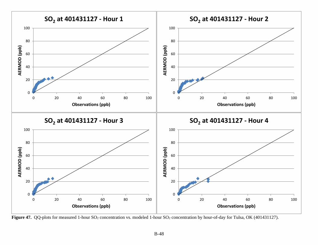
B-48


0

20

40

60

80

100

0 20 40 60 80 100

AER

MO

D (

pp

b)

Observations (ppb)

SO2 at 401431127 - Hour 1

0

20

40

60

80

100

0 20 40 60 80 100

AER

MO

D(p

pb

)

Observations (ppb)

SO2 at 401431127 - Hour 2

0

20

40

60

80

100

0 20 40 60 80 100

AER

MO

D(p

pb

)

Observations (ppb)

SO2 at 401431127 - Hour 3

0

20

40

60

80

100

0 20 40 60 80 100

AER

MO

D(p

pb

)

Observations (ppb)

SO2 at 401431127 - Hour 4

B-49


0

20

40

60

80

100

0 20 40 60 80 100

AER

MO

D(p

pb

)

Observations (ppb)

SO2 at 401431127 - Hour 5

0

20

40

60

80

100

0 20 40 60 80 100

AER

MO

D(p

pb

)

Observations (ppb)

SO2 at 401431127 - Hour 6

0

20

40

60

80

100

0 20 40 60 80 100

AER

MO

D(p

pb

)

Observations (ppb)

SO2 at 401431127 - Hour 7

0

20

40

60

80

100

0 20 40 60 80 100

AER

MO

D(p

pb

)

Observations (ppb)

SO2 at 401431127 - Hour 8

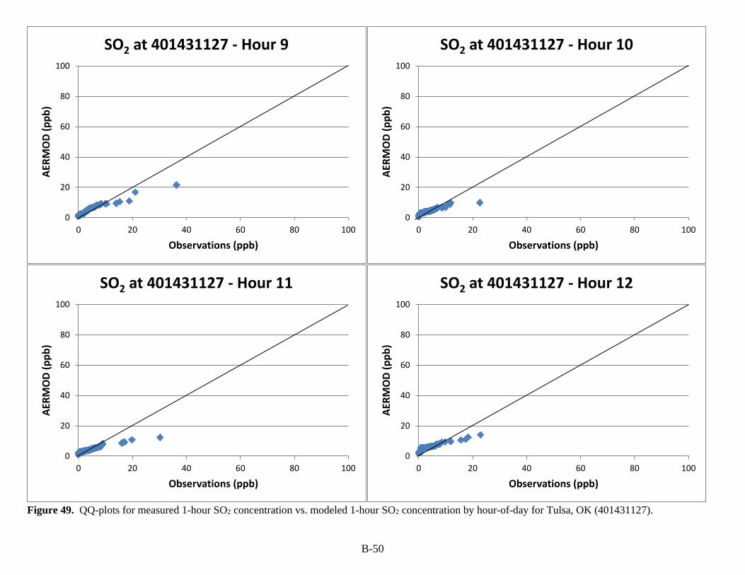
B-50


0

20

40

60

80

100

0 20 40 60 80 100

AER

MO

D(p

pb

)

Observations (ppb)

SO2 at 401431127 - Hour 9

0

20

40

60

80

100

0 20 40 60 80 100

AER

MO

D(p

pb

)

Observations (ppb)

SO2 at 401431127 - Hour 10

0

20

40

60

80

100

0 20 40 60 80 100

AER

MO

D(p

pb

)

Observations (ppb)

SO2 at 401431127 - Hour 11

0

20

40

60

80

100

0 20 40 60 80 100

AER

MO

D(p

pb

)

Observations (ppb)

SO2 at 401431127 - Hour 12

B-51


0

20

40

60

80

100

0 20 40 60 80 100

AER

MO

D (

pp

b)

Observations (ppb)

SO2 at 401431127 - Hour 13

0

20

40

60

80

100

0 20 40 60 80 100

AER

MO

D (

pp

b)

Observations (ppb)

SO2 at 401431127 - Hour 14

0

20

40

60

80

100

0 20 40 60 80 100

AER

MO

D (

pp

b)

Observations (ppb)

SO2 at 401431127 - Hour 15

0

20

40

60

80

100

0 20 40 60 80 100

AER

MO

D (

pp

b)

Observations (ppb)

SO2 at 401431127 - Hour 16

B-52


0

20

40

60

80

100

0 20 40 60 80 100

AER

MO

D (

pp

b)

Observations (ppb)

SO2 at 401431127 - Hour 17

0

20

40

60

80

100

0 20 40 60 80 100

AER

MO

D (

pp

b)

Observations (ppb)

SO2 at 401431127 - Hour 18

0

20

40

60

80

100

0 20 40 60 80 100

AER

MO

D (

pp

b)

Observations (ppb)

SO2 at 401431127 - Hour 19

0

20

40

60

80

100

0 20 40 60 80 100

AER

MO

D (

pp

b)

Observations (ppb)

SO2 at 401431127 - Hour 20

B-53


0

20

40

60

80

100

0 20 40 60 80 100

AER

MO

D (

pp

b)

Observations (ppb)

SO2 at 401431127 - Hour 21

0

20

40

60

80

100

0 20 40 60 80 100

AER

MO

D (

pp

b)

Observations (ppb)

SO2 at 401431127 - Hour 22

0

20

40

60

80

100

0 20 40 60 80 100

AER

MO

D (

pp

b)

Observations (ppb)

SO2 at 401431127 - Hour 23

0

20

40

60

80

100

0 20 40 60 80 100

AER

MO

D (

pp

b)

Observations (ppb)

SO2 at 401431127 - Hour 24

united states environmental protection … · environmental & occupational health ... lake...

Documents