Unit -1 Introduction

REVIEW OF DISCRETE TIME SIGNALS AND SYSTEMS Anything that carries some information can be called as signals. Some examples

are ECG, EEG, ac power, seismic, speech, interest rates of a bank, unemployment rate of a country, temperature, pressure etc. A signal is also defined as any physical quantity that varies with one or more

independent variables. A discrete time signal is the one which is not defined at intervals between two successive samples of a signal. It is represented as graphical, functional, tabular

representation and sequence. Some of the elementary discrete time signals are unit step, unit impulse, unit

ramp, exponential and sinusoidal signals (as you read in signals and systems). Classification of discrete time signals

Energy and Power signals

If the value of E is finite, then the signal x(n) is called energy signal.

If the value of the P is finite, then the signal x(n) is called Power signal.

Periodic and Non periodic signals A discrete time signal is said to be periodic if and only if it satisfies the condition X

(N+n) =x (n), otherwise non periodic

Symmetric (even) and Anti-symmetric (odd) signals The signal is said to be even if x(-n)=x(n) The signal is said to be odd if x(-n)= - x(n)

Causal and non causal signal The signal is said to be causal if its value is zero for negative values of ‘n’.

Some of the operations on discrete time signals are shifting, time reversal, time

scaling, signal multiplier, scalar multiplication and signal addition or multiplication.

Discrete time systems A discrete time signal is a device or algorithm that operates on discrete time

signals and produces another discrete time output. Classification of discrete time systems

Static and dynamic systems A system is said to be static if its output at present time depend on the input at present time only.

Causal and non causal systems A system is said to be causal if the response of the system depends on present and

past values of the input but not on the future inputs.

Linear and non linear systems A system is said to be linear if the response of the system to the weighted sum of inputs should be equal to the corresponding weighted sum of outputs of the

systems. This principle is called superposition principle. Time invariant and time variant systems

A system is said to be time invariant if the characteristics of the systems do not change with time.

Stable and unstable systems A system is said to be stable if bounded input produces bounded output only.

TIME DOMAIN ANALYSIS OF DISCRETE TIME SIGNALS AND SYSTEMS

Representation of an arbitrary sequence Any signal x(n) can be represented as weighted sum of impulses as given below

The response of the system for unit sample input is called impulse response of the

system h(n)

By time invariant property, we have

The above equation is called convolution sum.

Some of the properties of convolution are commutative law, associative law and distributive law.

Correlation of two sequences It is basically used to compare two signals. It is the measure of similarity between two signals. Some of the applications are communication systems, radar, sonar

etc. The cross correlation of two sequences x(n) and y(n) is given by

One of the important properties of cross correlation is given by

The auto correlation of the signal x(n) is given by

Linear time invariant systems characterized by constant coefficient difference equation The response of the first order difference equation is given by

The first part contain initial condition y(-1) of the system, the second part contains

input x(n) of the system. The response of the system when it is in relaxed state at n=0 or

y(-1)=0 is called zero state response of the system or forced response.

The output of the system at zero input condition x(n)=0 is called zero input

response of the system or natural response.

The impulse response of the system is given by zero state response of the system

The total response of the system is equal to sum of natural response and forced

responses.

FREQUENCY DOMAIN ANALYSIS OF DISCRETE TIME SIGNALS AND SYSTEMS A s we have observed from the discussion o f Section 4.1, the Fourier series

representation o f a continuous-time periodic signal can consist of an infinite number of frequency components, where the frequency spacing between two

successive harmonically related frequencies is 1 / T p, and where Tp is the fundamental period. Since the frequency range for continuous-time signals extends infinity on both

sides it is possible to have signals that contain an infinite number of frequency components.

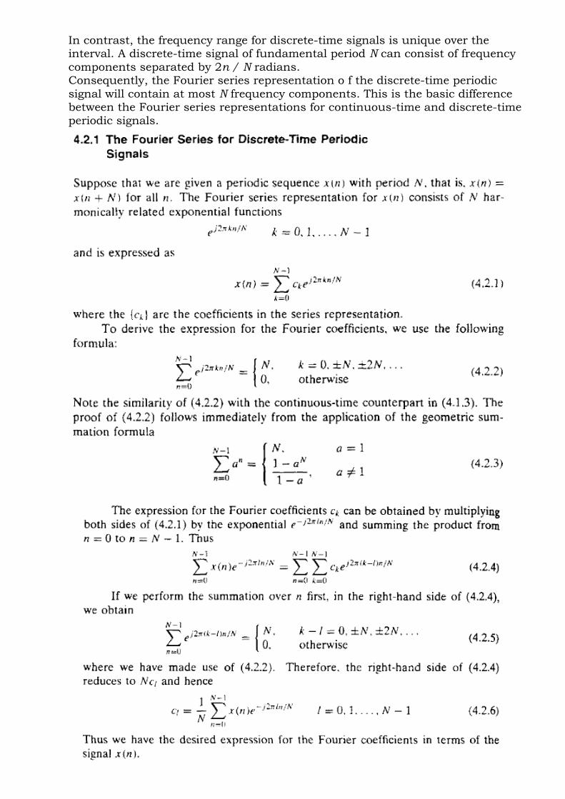
In contrast, the frequency range for discrete-time signals is unique over the interval. A discrete-time signal of fundamental period N can consist of frequency

components separated by 2n / N radians. Consequently, the Fourier series representation o f the discrete-time periodic

signal will contain at most N frequency components. This is the basic difference between the Fourier series representations for continuous-time and discrete-time

periodic signals.

PROPERTIES OF DFT:

LINEAR FILTERING METHODS BASED ON THE DFT

Since the D F T provides a discrete frequency representation o f a finite-duration Sequence in the frequency domain, it is interesting to exp lore its use as a

computational tool for linear system analysis and, especially, for linear filtering. We have already established that a system with frequency response H { w ) y w hen excited with an input signal that has a spectrum possesses an output

spectrum. The output sequence y(n) is determined from its spectrum via the inverse Fourier

transform. Computationally, the problem with this frequency domain approach is

that are functions o f the continuous variable. As a consequence, the computations cannot be done on a digital computer, since the computer can only

store and perform computations on quantities at discrete frequencies. On the other hand, the DFT does lend itself to computation on a digital computer.

In the discussion that follows, we describe how the DFT can be used to perform linear filtering in the frequency domain. In particular, we present a computational procedure that serves as an alternative to time-domain convolution.

In fact, the frequency-domain approach based on the DFT, is computationally m ore efficient than time-domain convolution due to the existence of efficient algorithms for computing the DFT . These algorithms, which are described

in Chapter 6, are collectively called fast Fourier transform (FFT) algorithms.

*******************************************************************************************