understanding the internet as-level structure

UNIVERSITY OF CALIFORNIA

Los Angeles

Understanding the Internet AS-level Structure

A dissertation submitted in partial satisfaction

of the requirements for the degree

Doctor of Philosophy in Computer Science

by

Ricardo V. Oliveira

2009

The dissertation of Ricardo V. Oliveira is approved.

Yingnian Wu

Beichuan Zhang

Mario Gerla

Songwu Lu

Leonard Kleinrock

Lixia Zhang, Committee Chair

University of California, Los Angeles

2009

ii

To my Parents . . .

for their unconditional love and affection

iii

TABLE OF CONTENTS

1 Introduction . . . . . . . . . . . . . . . . . . . . . . . . . . . . . . . . . 1

2 Background . . . . . . . . . . . . . . . . . . . . . . . . . . . . . . . . . 5

2.1 Internet Routing . . . . . . . . . . . . . . . . . . . . . . . . . . . . . 5

2.2 Inter-domain Connectivity and Peering . . . . . . . . . . . . . . . . . 7

2.3 Ground Truth vs. Observed Map . . . . . . . . . . . . . . . . . . . . 9

3 Topology Liveness and

Completeness Problems . . . . . . . . . . . . . . . . . . . . . . . . . . . . 13

4 A Solution to the Liveness Problem . . . . . . . . . . . . . . . . . . . . 18

4.1 An Empirical Model of Observed Topology Dynamics . . . . . . . . 18

4.1.1 Data Sets . . . . . . . . . . . . . . . . . . . . . . . . . . . . 18

4.1.2 An Empirical Model . . . . . . . . . . . . . . . . . . . . . . 20

4.1.3 Comparison with router configuration files from a Tier-1 . . . 29

4.1.4 Comparison with Internet Registry Data . . . . . . . . . . . . 31

4.1.5 Evaluation of Traceroute Data . . . . . . . . . . . . . . . . . 32

4.2 Applications . . . . . . . . . . . . . . . . . . . . . . . . . . . . . . . 37

4.2.1 More Accurate View of the Topology . . . . . . . . . . . . . 38

4.2.2 Evaluating Theoretical Models . . . . . . . . . . . . . . . . . 42

4.2.3 Characterizing Evolution Trends . . . . . . . . . . . . . . . . 44

4.3 Discussion . . . . . . . . . . . . . . . . . . . . . . . . . . . . . . . . 47

iv

5 Quantifying the Topology (in)Completeness . . . . . . . . . . . . . . . . 51

5.1 Data Sets . . . . . . . . . . . . . . . . . . . . . . . . . . . . . . . . 51

5.2 Establishing the Ground Truth . . . . . . . . . . . . . . . . . . . . . 53

5.3 Case studies . . . . . . . . . . . . . . . . . . . . . . . . . . . . . . . 58

5.3.1 Tier-1 Network . . . . . . . . . . . . . . . . . . . . . . . . . 59

5.3.2 Tier-2 Network . . . . . . . . . . . . . . . . . . . . . . . . . 62

5.3.3 Abilene and Geant . . . . . . . . . . . . . . . . . . . . . . . 65

5.3.4 Content provider . . . . . . . . . . . . . . . . . . . . . . . . 67

5.3.5 Simple stubs . . . . . . . . . . . . . . . . . . . . . . . . . . 70

5.4 Completeness of the public view . . . . . . . . . . . . . . . . . . . . 71

5.4.1 ”Public view” vs. ground truth . . . . . . . . . . . . . . . . . 71

5.4.2 Network Classification . . . . . . . . . . . . . . . . . . . . . 73

5.4.3 Coverage of the public view . . . . . . . . . . . . . . . . . . 77

5.5 Discussion . . . . . . . . . . . . . . . . . . . . . . . . . . . . . . . . 79

6 Path Exploration and Internet Topology . . . . . . . . . . . . . . . . . 82

6.1 BGP Path Exploration . . . . . . . . . . . . . . . . . . . . . . . . . . 82

6.2 Methodology and Data Set . . . . . . . . . . . . . . . . . . . . . . . 83

6.2.1 Data Set and Preprocessing . . . . . . . . . . . . . . . . . . . 85

6.2.2 Clustering Updates into Events . . . . . . . . . . . . . . . . . 86

6.2.3 Classifying Routing Events . . . . . . . . . . . . . . . . . . . 89

6.2.4 Comparing AS Paths . . . . . . . . . . . . . . . . . . . . . . 91

6.3 Characterizing Events . . . . . . . . . . . . . . . . . . . . . . . . . . 98

v

6.3.1 The Impact of Unstable Prefixes . . . . . . . . . . . . . . . . 104

6.4 Policies, Topology and Routing Convergence . . . . . . . . . . . . . 104

6.4.1 MRAI Timer . . . . . . . . . . . . . . . . . . . . . . . . . . 105

6.4.2 The Impact of Policy and Topology on Routing Convergence . 106

6.4.3 Origin of Fail-down Events . . . . . . . . . . . . . . . . . . . 111

6.4.4 Impact of Fail-down Convergence . . . . . . . . . . . . . . . 112

7 Prefix Hijacking and Internet Topology . . . . . . . . . . . . . . . . . . 115

7.1 Prefix Hijacking . . . . . . . . . . . . . . . . . . . . . . . . . . . . . 115

7.2 Hijack Evaluation Metrics . . . . . . . . . . . . . . . . . . . . . . . 116

7.3 Evaluating Hijacks . . . . . . . . . . . . . . . . . . . . . . . . . . . 119

7.3.1 Simulation Setup . . . . . . . . . . . . . . . . . . . . . . . . 119

7.3.2 Characterizing Topological Resilience . . . . . . . . . . . . . 120

7.3.3 Factors Affecting Resilience . . . . . . . . . . . . . . . . . . 122

7.4 Prefix Hijack Incidents in the Internet . . . . . . . . . . . . . . . . . 125

7.4.1 Case I: Prefix Hijacks by AS-27506 . . . . . . . . . . . . . . 125

7.4.2 Case II: Prefix Hijacks by AS-9121 . . . . . . . . . . . . . . 128

7.5 Discussion . . . . . . . . . . . . . . . . . . . . . . . . . . . . . . . . 131

8 Related Work . . . . . . . . . . . . . . . . . . . . . . . . . . . . . . . . 134

8.1 Internet Topology Modeling . . . . . . . . . . . . . . . . . . . . . . 134

8.2 Path Exploration . . . . . . . . . . . . . . . . . . . . . . . . . . . . 135

8.3 Prefix Hijacking . . . . . . . . . . . . . . . . . . . . . . . . . . . . . 137

vi

9 Conclusion . . . . . . . . . . . . . . . . . . . . . . . . . . . . . . . . . 139

References . . . . . . . . . . . . . . . . . . . . . . . . . . . . . . . . . . . 141

vii

LIST OF FIGURES

2.1 Route propagation. . . . . . . . . . . . . . . . . . . . . . . . . . . . 7

2.2 A sample IXP. ASes A through G connect to each other through a

layer-2 switch in subnet 195.69.144/24. . . . . . . . . . . . . . . . . 8

2.3 A set of interconnected ASes, each node represent an AS. (a) shows

an example of hidden links, and (b) an example of invisible links. . . . 10

3.1 Observing Topology Over Time . . . . . . . . . . . . . . . . . . . . 14

4.1 Number of links captured by different sets of monitors . . . . . . . . 19

4.2 Number of monitors in RouteViews and RIPE-RIS combined . . . . . 19

4.3 Number of links, Tier-1 monitor with different starting times . . . . . 19

4.4 Visible links seen by all monitors . . . . . . . . . . . . . . . . . . . . 19

4.5 Link disappearance period . . . . . . . . . . . . . . . . . . . . . . . 21

4.6 Link disappearance period, by all monitors . . . . . . . . . . . . . . . 21

4.7 Observation period as a function of confidence level for links . . . . . 24

4.8 Node birth from RIR . . . . . . . . . . . . . . . . . . . . . . . . . . 24

4.9 Link birth from IRR . . . . . . . . . . . . . . . . . . . . . . . . . . . 27

4.10 Link death from IRR . . . . . . . . . . . . . . . . . . . . . . . . . . 27

4.11 Visible links in Skitter, λ = 0.00598, b = 39.86. . . . . . . . . . . . . 28

4.12 Comparison between routers’ config files connectivity and BGP data

(cumulative) from a Tier-1 network. . . . . . . . . . . . . . . . . . . 30

4.13 Comparison of appearance times between routers’ config files and BGP

data of a Tier-1 network. . . . . . . . . . . . . . . . . . . . . . . . . 30

viii

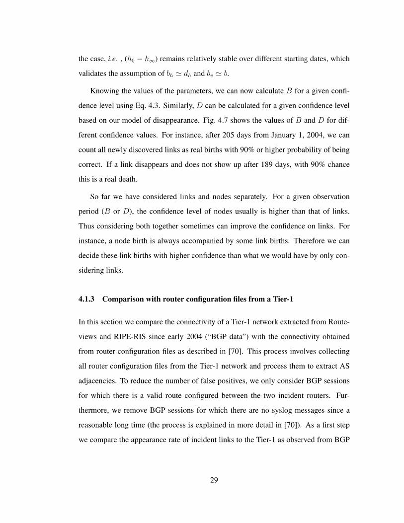
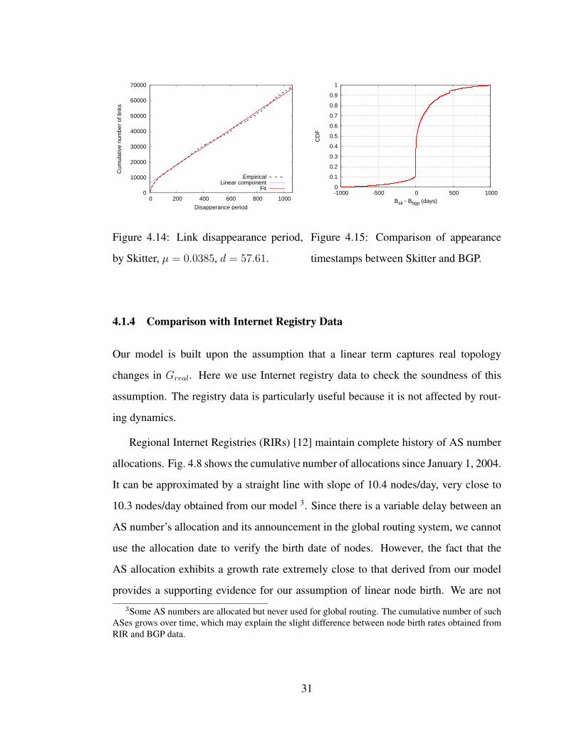
4.14 Link disappearance period, by Skitter, µ = 0.0385, d = 57.61. . . . . 31

4.15 Comparison of appearance timestamps between Skitter and BGP. . . . 31

4.16 Comparison of disappearance timestamps between Skitter and BGP. . 33

4.17 Number of reachable addresses in Skitter destination list. . . . . . . . 33

4.18 Trade-off between liveness and completeness for topology snapshot. . 37

4.19 Fraction of multi-homed customers. . . . . . . . . . . . . . . . . . . 37

4.20 Attachment probability distribution for a target node degree. . . . . . 38

4.21 Model evaluation . . . . . . . . . . . . . . . . . . . . . . . . . . . . 41

4.22 Node net growth . . . . . . . . . . . . . . . . . . . . . . . . . . . . . 41

4.23 Link net growth . . . . . . . . . . . . . . . . . . . . . . . . . . . . . 44

4.24 Net growth of node wirings. . . . . . . . . . . . . . . . . . . . . . . 44

4.25 Frequency of link changes . . . . . . . . . . . . . . . . . . . . . . . 45

4.26 Number of collected links in DIMES. . . . . . . . . . . . . . . . . . 48

4.27 Diurnal pattern of new link appearances. . . . . . . . . . . . . . . . . 48

4.28 Weekly pattern of new link appearances. . . . . . . . . . . . . . . . . 49

4.29 Link growth for Abilene (AS11537). . . . . . . . . . . . . . . . . . . 49

5.1 Output of “show ip bgp summary” command. . . . . . . . . . . . . . 54

5.2 Configuring remote BGP peerings. R0 and R2 are physically directly

connected, while R1 and R3 are not. . . . . . . . . . . . . . . . . . . 54

5.3 Connectivity of the Tier-1 network (since 2004). . . . . . . . . . . . . 58

5.4 Connectivity of the Tier-1 network (since 2007). . . . . . . . . . . . . 58

5.5 Capturing the connectivity of the Tier-1 network through table snap-

shots and updates. . . . . . . . . . . . . . . . . . . . . . . . . . . . . 59

ix

5.6 Tier-2 network connectivity. . . . . . . . . . . . . . . . . . . . . . . 59

5.7 Capturing Tier-2 network connectivity through table snapshots and up-

dates. . . . . . . . . . . . . . . . . . . . . . . . . . . . . . . . . . . 60

5.8 Abilene connectivity. . . . . . . . . . . . . . . . . . . . . . . . . . . 60

5.9 Projection of the number of peer ASes of a representative content

provider. . . . . . . . . . . . . . . . . . . . . . . . . . . . . . . . . . 68

5.10 Customer-provider links can be revealed over time, but downstream

peer links are invisible to upstream monitors. . . . . . . . . . . . . . 74

5.11 Distribution of number of downstream customers per AS. . . . . . . . 74

5.12 Example of a prefix hijack scenario where AS2 announces prefix p

belonging to AS1. Because of the invisible peer link AS2–AS3, the

number of ASes affected by the attack is underestimated. . . . . . . . 74

6.1 Path exploration triggered by a fail-down event. . . . . . . . . . . . . 83

6.2 CCDF of inter-arrival times of BGP updates for the 8 beacon prefixes

as observed from the 50 monitors. . . . . . . . . . . . . . . . . . . . 88

6.3 Difference in number of events per [monitor,prefix] for T=2 and 8 min-

utes, relatively to T=4 minutes, during one month period. . . . . . . . 88

6.4 Event taxonomy. . . . . . . . . . . . . . . . . . . . . . . . . . . . . 89

6.5 Usage time per ASPATH-Prefix for router 12.0.1.63, Jan 2006. . . . . 93

6.6 Validation of path preference metric. . . . . . . . . . . . . . . . . . . 95

6.7 Comparison between Ccorrect,Cequal and Cwrong of length , policy and

usage time metrics for (a) Tup and (b) Tdown events of beacon prefixes. 95

6.8 Comparison between accuracy of length, policy and usage time metrics. 95

6.9 Number of Tdown events per monitor. . . . . . . . . . . . . . . . . . . 99

x

6.10 Duration of events for January 2006. . . . . . . . . . . . . . . . . . . 100

6.11 Duration of events for February 2006. . . . . . . . . . . . . . . . . . 100

6.12 Number of Updates per Event, January 2006. . . . . . . . . . . . . . 101

6.13 Number of Unique Paths Explored per Event, January 2006. . . . . . 101

6.14 Duration of events for unstable prefixes, January 2006. . . . . . . . . 101

6.15 Duration of events for stable prefixes, January 2006. . . . . . . . . . . 101

6.16 Determining MRAI configuration. . . . . . . . . . . . . . . . . . . . 106

6.17 Duration of Tdown events as seen by monitors at different tiers. . . . . 109

6.18 Number of unique paths explored during Tdown as seen by monitors at

different tiers. . . . . . . . . . . . . . . . . . . . . . . . . . . . . . . 109

6.19 Topology example. . . . . . . . . . . . . . . . . . . . . . . . . . . . 110

6.20 Duration of Tdown events observed and originated in different tiers. . . 110

6.21 Number of paths explored during Tdown events observed and originated

in different tiers. . . . . . . . . . . . . . . . . . . . . . . . . . . . . . 110

6.22 Median of duration of Tdown events observed and originated in differ-

ent tiers. . . . . . . . . . . . . . . . . . . . . . . . . . . . . . . . . . 110

6.23 Number of Tdown events over time. . . . . . . . . . . . . . . . . . . . 112

6.24 Case where Tdown convergence disrupts data delivery. . . . . . . . . . 114

7.1 Hijack scenario. . . . . . . . . . . . . . . . . . . . . . . . . . . . . . 117

7.2 Distribution of node resilience. . . . . . . . . . . . . . . . . . . . . . 121

7.3 Resilience of nodes in different tiers. . . . . . . . . . . . . . . . . . . 121

7.4 Understanding resilience of tier-1 nodes . . . . . . . . . . . . . . . . 124

7.5 Resilience of nodes with different number of Tier-1 providers. . . . . 124

xi

7.6 Case study: AS-27506 as false origin . . . . . . . . . . . . . . . . . . 127

7.7 Case studies with AS-9121 as false origin . . . . . . . . . . . . . . . 130

xii

LIST OF TABLES

4.1 Model Parameters . . . . . . . . . . . . . . . . . . . . . . . . . . . . 25

4.2 Comparison Between Stub and Transit changes. . . . . . . . . . . . . 41

5.1 IXP membership data, July 2007. . . . . . . . . . . . . . . . . . . . . 53

5.2 Connectivity of stub networks. . . . . . . . . . . . . . . . . . . . . . 71

5.3 Coverage of BGP monitors. . . . . . . . . . . . . . . . . . . . . . . . 78

5.4 Coverage of BGP monitors for different network types. . . . . . . . . 79

6.1 Event Statistics for Jan 2006 (31 days) . . . . . . . . . . . . . . . . . 99

6.2 Event Statistics for Feb 2006 (28 days) . . . . . . . . . . . . . . . . . 100

6.3 Tdown Events by Origin AS . . . . . . . . . . . . . . . . . . . . . . . 113

xiii

ACKNOWLEDGMENTS

First and foremost, I would like to acknowledge my dissertation advisor Dr. Lixia

Zhang for her constant support and guidance through out my dissertation. I would also

like to acknowledge Dr. Mohit Lad for his infinite patience, helpful discussions and

relentless support. I am also grateful to Dr. Beichuan Zhang for contributing to the

original idea of modeling topology evolution by a birth/death model, Dr. Walter Will-

inger and Dr. Dan Pei for their guidance during the AT&T internship, Dr. Christophe

Diot for his guidance during Thomson internship and Dr. Qingming Ma for his super-

vision while at Juniper Networks. I would like to extend a special note of thanks to

Verra Morgan for her time and support during my Ph.D. Finally, various friends and

colleagues have played an important role during my Ph.D., notable among them are

Dr. Vasilis Pappas, Dr. Dan Massey, Rafit Izhak-Ratzin, Cesar Marcondes, Cassio

Lopes, Niko Palaskas, Bruno Miranda, Leonardo Alves and my sister Raquel Oliveira.

Finally, I would like to acknowledge the portuguese ”Fundacao para a Ciencia e Tec-

nologia” (FCT) for their scholarships under which my Phd work was supported.

xiv

VITA

1978 Born, Povoa de Varzim, Portugal

2001 B.E. Electrical Engineering, Faculty of Engineering of Porto Uni-

versity, Portugal.

2001–2002 Software developer, Oberonsis, Portugal.

2002–2003 Telecommunications Engineer, TMN, Portugal.

2005 M.Sc. Computer Science, University of California, Los Angeles.

2007 Intern at AT&T Labs Research.

2007 Intern at Thomson, Paris.

2008 Intern at Juniper Networks.

PUBLICATIONS

1. Ricardo Oliveira, Dan Pei , Walter Willinger, Beichuan Zhang, Lixia Zhang, ”The

(in)Completeness of the Observed Internet AS-level Structure”, to appear in IEEE/ACM

Transactions on Networking

2. Ricardo Oliveira, Beichuan Zhang, Dan Pei, Lixia Zhang, ”Quantifying Path Ex-

ploration in the Internet”, to appear in IEEE/ACM Transactions on Networking, June

xv

2009

3. Italo Cunha, Fernando Silveira, Ricardo Oliveira, Renata Teixeira, Christophe Diot,

”Uncovering Artifacts of Flow Measurement Tools”,Passive and Active Measurement

Conference, April 2009

4. He Yan, Ricardo Oliveira, Kevin Burnett, Dave Matthews, Lixia Zhang, Dan

Massey, ”BGPmon: A real-time, scalable, extensible monitoring system”, Cyberse-

curity Applications and Technologies Conference for Homeland Security (CATCH),

March 2009

5. Ricardo Oliveira, Fernando Silveira, Renata Teixeira, Christophe Diot, ”The elusive

Effect of Routing Dynamics on Traffic Anomalies”, Technical Report, Thomson, CR-

PRL-2008-02-0001

6. Ricardo Oliveira, Dan Pei , Walter Willinger, Beichuan Zhang, Lixia Zhang, ”Quan-

tifying the Completeness of the Observed Internet AS-level Structure”, Technical Re-

port, UCLA CS Department, TR 080026, September 2008

7. Ying-Ju Chi, Ricardo Oliveira , Lixia Zhang, ”Cyclops: The Internet AS-level

Observatory”, ACM SIGCOMM Computer Communication Review (CCR), October

2008

8. Ricardo Oliveira, Ying-Ju Chi, Mohit Lad, Lixia Zhang, ”Cyclops: The Internet

AS-level Observatory”, NANOG 43, Brooklyn, New York, June 2008

xvi

9. Ricardo Oliveira, Dan Pei, Walter Willinger, Beichuan Zhang, Lixia Zhang, ”In

Search of the elusive Ground Truth: The Internet’s AS-level Connectivity Structure”,

ACM SIGMETRICS, Annapolis, USA, June 2008

10. Ricardo Oliveira, Mohit Lad, Beichuan Zhang, Lixia Zhang, ”Geographically

Informed Inter-Domain Routing”, in IEEE ICNP, Beijing, China, October 2007

11. Mohit Lad, Ricardo Oliveira, Dan Massey, Lixia Zhang, ”Inferring the Origin of

Routing Changes using Link Weights”, in IEEE ICNP, Beijing, China, October 2007

12. Ricardo Oliveira, Beichuan Zhang, Lixia Zhang, ”Observing the Evolution of

Internet AS Topology”, in ACM SIGCOMM, Kyoto, Japan, August 2007

13. Ricardo Oliveira, Ying-Ju Chi, Ioannis Pefkianakis, Mohit Lad, Lixia Zhang, ”Vi-

sualizing Internet Topology Dynamics with Cyclops”, in ACM SIGCOMM (poster

session), Kyoto, Japan, August 2007

14. Mohit Lad, Ricardo Oliveira, Beichuan Zhang, Lixia Zhang, ”Understanding the

Resiliency of Internet Topology Against False Origin Attacks”, in IEEE/IFIP DSN,Edinburgh,

UK, June 2007

15. Ricardo Oliveira, Beichuan Zhang, Dan Pei, Rafit Izhak-Ratzin, Lixia Zhang,

”Quantifying Path Exploration in the Internet”, ACM SIGCOMM/USENIX Internet

Measurement Conference(IMC), Rio de Janeiro, Brazil, October 2006

16. Mohit Lad, Ricardo Oliveira, Beichuan Zhang, Lixia Zhang, ”Understanding the

xvii

Impact of Prefix Hijacks in Internet Routing ”, ACM SIGCOMM (poster session),

Pisa, Italy, September 2006

17. Beichuan Zhang, Vamsi Kambhampati, Daniel Massey, Ricardo Oliveira, Dan

Pei, Lan Wang, Lixia Zhang ”A Secure and Scalable Internet Routing Architecture

(SIRA)”, ACM SIGCOMM (poster session), Pisa, Italy, September 2006

18. Ricardo Oliveira, Mohit Lad, Beichuan Zhang, Dan Pei, Daniel Massey, Lixia

Zhang, ”Placing BGP Monitors in the Internet”, Technical Report, UCLA CS Depart-

ment, TR 060017, May 2006

19. Vidyut Samanta, Ricardo Oliveira, Advait Dixit, Parixit Aghera, Petros Zerfos,

Songwu Lu, ”Impact of Video Encoding Parameters on Dynamic Video Transcoding”,

in IEEE COMSWARE, Delhi, India, January 2006.

20. Ricardo Oliveira, Rafit Izhak-Ratzin, Beichuan Zhang, Lixia Zhang,”Measurement

of Highly Active Prefixes in BGP”, in IEEE GLOBECOM, St. Louis, USA, November

2005.

xviii

ABSTRACT OF THE DISSERTATION

Understanding the Internet AS-level Structure

by

Ricardo V. OliveiraDoctor of Philosophy in Computer Science

University of California, Los Angeles, 2009

Professor Lixia Zhang, Chair

The Internet is a vast distributed system consisting of a myriad of independent net-

works interconnected to each other by business relationships. The border gateway

protocol is the glue that keeps this structure connected. Characterizing and modeling

the Internet topology is important to our understanding of Internet routing and its in-

terplay with technical, economic and social forces. In this thesis we address several

challenges that emerge when studying the Internet connectivity. First, not all the ob-

served changes in connectivity correspond to actual changes in the topology. There

are changes that may be caused by transient routing dynamics while others are real

topology changes. The problem of distinguishing between these two types of changes

is non-trivial, and we call it the liveness problem. We propose a solution to this prob-

lem based on a birth/death model of observed links. This solution allows to accurately

detect the permanent changes in the Internet topology graph and measure topology

dynamics in an accurate way. The second problem in obtaining accurate topology

models is the completeness problem, which consists in establishing how much of the

real topology is missing from the observed data. We address the completeness prob-

lem by defining some bounds on how (in)complete is the graph provided by the current

observation. The results using ground truth information obtained from a Tier-1 ISP in-

xix

dicate that the observed Internet graph contains most of the customer-provider links,

but may be missing the vast majority of the peer-peer links. Finally, we study how

protocol properties such as routing convergence and resilience to prefix hijack attacks

depend on the connectivity and relationship between networks. We find that networks

at the border of the Internet undergo more severe path exploration because of the higher

number of paths available to reach other destinations. On the other hand, we show that

Tier-1 networks have the fastest convergence time because of the limited number of

alternative routes. In terms of prefix hijack attacks, we surprisingly find that Tier-1

networks at the core of the Internet are vulnerable to hijack attacks from customers

because of the business nature of BGP route selection. Based on our observations, we

formulate a connectivity recommendation for ISPs to increase their resiliency to these

type of attacks.

xx

CHAPTER 1

Introduction

The Internet has been evolving rapidly over recent years, much like a living organism,

and its topology has become more complex. Characterizing the structure and evolu-

tion trends of the Internet topology is an important research topic for several reasons. It

provides an essential input to the understanding of limitations of existing routing pro-

tocols, the evaluations of new designs, as well as the projection of future needs; and it

will help advance our understanding of the interplay between networking technology,

the resulting topology, and the economic forces behind them.

Many research projects have used a graphic representation of the Internet AS-level

topology, where nodes represent entire autonomous systems (ASes) and two nodes

are connected if and only if the two ASes are engaged in a business relationship to

exchange data traffic. Due to the Internet’s decentralized architecture, however, this

AS-level construct is not readily available and obtaining accurate AS maps has re-

mained an active area of research. A common feature of all the AS maps that have

been used by the research community is that they have been inferred from either BGP-

based or traceroute-based data. Unfortunately, both types of measurements are more a

reflection of what we can measure than what we really would like to measure, resulting

in fundamental limitations as far as their ability to reveal the Internet’s true AS-level

connectivity structure is concerned.

While these limitations inherent in the available data have long been recognized,

there has been little effort in assessing the degree of completeness, accuracy, and am-

1

biguity of the resulting AS maps. Although it is relatively easy to collect a more or less

complete set of ASes, it has proven difficult, if not impossible, to collect the complete

set of inter-AS links. The sheer scale of the AS-level Internet makes it infeasible to

install monitors everywhere or crawl the topology exhaustively. At the same time, big

stakeholders of the AS-level Internet, such as Internet service providers and large con-

tent providers, tend to view their AS connectivity as proprietary information and are in

general unwilling to disclose it. As a result, the quality of the currently used AS maps

has remained by and large unknown. Yet numerous projects [37, 55, 59, 20, 31, 29, 91]

have been conducted using these maps of unknown quality, causing serious scientific

and practical concerns in terms of the validity of the claims made and accuracy of the

results reported.

Obtaining accurate and complete Internet topology data is a challenging task. First,

the observed AS topology snapshots only capture a subset of the real Internet topology

[27, 99, 60, 77, 96, 70]. This is referred as the completeness problem. The incom-

pleteness of the observed AS topology stems from the fact that our main source of

connectivity data are BGP routing tables (Border Gateway Protocol), and BGP was

designed to propagate routing information, not AS adjacencies. In BGP, only the best

path is propagated to neighbors, and not all neighbors receive all routes, therefore it’s

only natural that there is missing connectivity information when using a limited num-

ber of vantage points. By using ground truth information of a Tier-1 ISP, we quantify

to some extent the degree of incompleteness of the observed topology. We find that

current set of vantage points are able to capture the totality of customer-provider links,

but as much as 90% of the peer links are still escaping from observation. The invisible

peer links exist mainly between nodes at the border of the network.

Second, a new problem arises when we try to measure topology changes over time:

the changes in the observed topology do not necessarily reflect the changes in the

2

real topology and vice versa. Because the observed topology is normally inferred

from routing or data paths, its changes can be due to either real topology changes or

transient routing dynamics (e.g. , caused by link failures or router crashes). Therefore

the challenge is, given all the changes in the observed topology over time, how to

differentiate those caused by real topology changes from those caused by transient

routing dynamics, which we call the liveness problem. Only after solving the liveness

problem can we provide empirical topology evolution data such as when and where

an AS or an inter-AS link is added or removed from the Internet. In this thesis we

develop a solution to the liveness problem based on the analysis of available data. Our

analysis shows that the effect of transient routing dynamics on the observed topology

decreases exponentially over time, and the real topology changes can be modeled as

the combination of a constant-rate birth process and a constant-rate death process.

There are several properties of BGP that depend on the structure of the Internet

topology. In this thesis we study two of these properties: path exploration and re-

siliency to prefix hijacks. Before declaring a destination unreachable, BGP explores

all backup paths until it finds a valid one. We call this process path exploration. In or-

der to reduce delays and data loss during routing convergence, path exploration should

happen as fast as possible. We show that path exploration depends on the number of

alternative paths between the source and the destination, and that nodes at the border

of the network with more alternative paths will experience more severe convergence

delays than nodes at the core of the network. Other protocol property(or deficiency)

that depends heavily on the topology is the resiliency of a node to prefix hijacks. A

prefix hijack attack happens when a network X starts announcing address space that

belongs to a network Y . The end result is that a fraction of the traffic will be deviated

to the false origin. In some cases the false origin can even intercept the traffic and

send it back to the true origin. After conducting a set of Internet scale simulations we

find that networks connected with multiple Tier-1s are the most resilient to this type of

3

attacks. Furthermore, we also surprisingly find that Tier-1s at the core of the network

are more vulnerable to prefix hijacks launched by its customers because of the policy

factor in BGP route selection.

The main contributions of this dissertation can be summarized as follows. First, we

formulate the topology liveness problem and propose a solution for it, this is described

in Chapter 4. Second, we investigate the completeness of the observed AS topology

by quantifying and explaining the reasons why AS adjacencies are missing from com-

monly used data sources, which is described in Chapter 5. Third, in Chapter 6 we

establish the dependency between the convergence of BGP routes and the topological

location of both the monitor and the origin of the routes. Lastly, in Chapter 7 we show

how the resiliency of networks to prefix hijack depends on how close to the Tier-1 core

each network is connected.

4

CHAPTER 2

Background

In this section we present the relevant background on Internet routing and relationships

between different networks.

2.1 Internet Routing

The Internet consists of more than thirty thousand networks called “Autonomous Sys-

tems” (AS). Each AS is represented by a unique numeric ID known as its AS num-

ber, and may advertise one or more IP address prefixes. For example, the prefix

131.179.0.0/16 represents a range of 216 IP addresses belonging to AS-52 (UCLA).

Internet Registries such as ARIN and RIPE assign prefixes to organizations, who then

become the owner of the prefixes. Automonous Systems run the Border Gateway Pro-

tocol (BGP) [78] to propagate prefix reachability information among themselves. In

the rest of the thesis, we abstract an autonomous system into a single entity called AS

node or node, and the BGP connection between two autonomous systems as AS link or

simply link.

BGP uses routing update messages to propagate routing changes. As a path-vector

routing protocol, BGP lists the entire AS path to reach a destination prefix in its rout-

ing updates. Route selection and announcement in BGP are determined by networks’

routing policies, in which the business relationship between two connected ASes plays

a major role. AS relationships can be generally classified as customer-provider or peer-

5

peer1. In a customer-provider relationship, the customer AS pays the provider AS for

access service to the rest of the Internet. The peer-peer relationship does not usually

involve monetary flow; The two peer ASes exchange traffic between their respective

customers only. Usually a customer AS does not forward traffic between its providers,

nor does a peer AS forward traffic between two other peers. For example in Figure 2.1,

AS-1 is a customer of AS-2 and AS-3, and hence would not want to be a transit be-

tween AS-2 and AS-3, since it would be pay both AS-2 and AS-3 for traffic exchange

between themselves. This results in the so-called valley-free BGP paths [39] generally

observed in the Internet. When ASes choose their best path, they usually follow the

order of customer routes, peer routes, and provider routes. This policy of no valley

prefer customer is generally followed by most networks in the Internet. As we will see

later, the no valley prefer customer policy plays an important role in determining the

impact of prefix hijacks and hence we present a simple example to illustrate how this

policy works.

Figure 2.1 provides a simple example illustrating route selection and propagation.

AS-1 announces a prefix (e.g. 131.179.0.0/16) to its upstream service providers AS-2

and AS-3. The AS announcing a prefix to the rest of the Internet is called the origin

AS of that prefix. Each of these providers then prepends its own AS number to the

path and propagates the path to their neighbors. Note that AS-3 receives paths from its

customer, AS-1, as well as its peer, AS-2, and it selects the customer path over the peer

path thus advertising the path {3 1} to its neighbors AS-4 and AS-5. AS-5 receives

routes from AS-2 and AS-3 and we assume AS-5 selects the route announced by AS-

3 and announces the path {5 3 1} to its customer AS-6. In general, an AS chooses

which routes to import from its neighbors and which routes to export to its neighbors

based on import and export routing policies. An AS receiving multiple routes picks

1Sometimes the relationship between two AS nodes can be “siblings,” usually because they belongto the same organization.

6

4

2

1

3

6

5

Provider CustomerPeer Peer 2-1

1

1

5-3-13-1

Tier-1

3-1

2-1

2-1

Figure 2.1: Route propagation.

the best route based on policy preference. Metrics such as path length and other BGP

parameters are used in route selection if the policy is the same for different routes. The

BGP decision process also contains many more parameters that can be configured to

mark the preference of routes. A good explanation of these parameters can be found

in [41].

2.2 Inter-domain Connectivity and Peering

As a path-vector protocol, BGP includes in its routing updates the entire AS-level path

to each prefix, which can be used to infer the AS-level connectivity. Projects such as

RouteViews [15] and RIPE-RIS [14] host multiple data collectors that establish BGP

sessions with operational routers, which we term monitors, in hundreds of ASes to

obtain their BGP forwarding tables and routing updates over time.

Among all the ASes, less than 10% are transit networks, and the rest are stub net-

works. A transit network is an Internet Service Provider (ISP) whose business is to

provide packet forwarding service between other networks. Stub networks, on the

7

FC

D E

G

A

B

Layer-2 cloud

IXP

195.69.144.1

195.69.144.2195.69.144.7

195.69.144.3

195.69.144.4195.69.144.5

195.69.144.6

Figure 2.2: A sample IXP. ASes A through G connect to each other through a layer-2

switch in subnet 195.69.144/24.

other hand, do not forward packets for other networks. In the global routing hier-

archy, stub networks are at the bottom or at the edge, and need transit networks as

their providers to reach the rest of the Internet. Transit networks may have their own

providers and peers, and are usually described as different tiers, e.g., regional ISPs,

national ISPs, and global ISPs. At the top of this hierarchy are a dozen or so tier-1

ISPs, which connect to each other in a fully mesh to form the core of the global rout-

ing infrastructure. The majority of stub networks today multi-home with more than

one provider, and some stub networks also peer with each other. In particular, content

networks, e.g., networks supporting search engines, e-commerce, and social network

sites, tend to peer with a large number of other networks.

Peering is a delicate but also important issue in inter-domain connectivity. A

network has incentives to peer with other networks to reduce the traffic sent to its

providers, hence saving operational costs. But peering also comes with its own issues.

For ISPs, besides additional equipment and management cost, they also do not want

to establish peer-peer relationships with potential customers. Therefore ISPs in gen-

8

eral are very selective in choosing their peers. Common criteria include number of

co-locations, ratio of inbound and outbound traffic, and certain requirements on prefix

announcements [2, 1]. In recent years, with the fast growth of available content in the

Internet, content networks have been keen on peering with other networks to bypass

their providers. Because they have no concern regarding transit traffic or potential cus-

tomers, content networks generally have an open peering policy and peer with a large

number of other networks.

AS peering can be realized through either private peering or public peering. A

private peering is a dedicated connection between two networks. It provides dedi-

cated bandwidth, makes troubleshooting easier, but has a higher cost. Public peering

usually happens at the Internet Exchange Points (IXPs), which are third-party main-

tained physical infrastructures that enable physical connectivity between their mem-

ber networks2. Currently most IXPs connect their members through a shared layer-2

switching fabric (or layer-2 cloud). Figure 2.2 shows an IXP that interconnects ASes

A through G using a subnet 195.69.144.0/24. Though an IXP provides physical con-

nectivity among all participants, it is up to individual networks to decide with whom to

establish BGP sessions. It is often the case that one network only peers with some of

the other participants in the same IXP. Public peering has a lower cost but its available

bandwidth capacity between any two parties can be limited. However, with the recent

increase in bandwidth capacity, we have seen a trend to migrate private peerings to

public peerings.

2.3 Ground Truth vs. Observed Map

To study AS-level connectivity, we need a clear definition on what constitutes an inter-

AS link. A link between two ASes exists if the two ASes have a contractual agreement

2Note that private and public peering can happen in the same physical facility.

9

5

2

4

1

9

6 7

83

10

Provider CostumerPeer Peer

Best path

(a) (b)

p0 p1 p2

Figure 2.3: A set of interconnected ASes, each node represent an AS. (a) shows an

example of hidden links, and (b) an example of invisible links.

to exchange traffic over one or multiple BGP sessions. The ground truth of the Inter-

net AS-level connectivity is the complete set of AS links. As the Internet evolves, its

AS-level connectivity also changes over time. We use Greal(t) to denote the ground

truth of the entire Internet AS-level connectivity at time t.

Ideally if each ISP maintains an up-to-date list of its AS links and makes the list ac-

cessible, obtaining the ground truth would be trivial. However, such a list is proprietary

and rarely available, especially for large ISPs with a large and changing set of links.

In this thesis, we derive the ground truth of several individual networks whose data

is made available to us, including their router configurations, syslogs, BGP command

outputs, as well as personal communications with the operators.

From router configurations, syslogs and BGP command outputs, we can infer

whether there is a working BGP session, i.e., a BGP session that is in the established

state as specified in RFC 4271 [78]. We assume there is a link between two ASes if

there is at least one working BGP session between them. However if all the BGP ses-

sions between two ASes are down at the moment of data collection, the link may not

10

appear in the ground truth on that particular day, even though the two ASes have a valid

agreement to exchange traffic. Fortunately we have continuous daily data going back

for years, thus the problem of missing links due to transient failures should be neg-

ligible. When inferring connectivity from router configurations, extra care is needed

to remove stale BGP sessions, i.e. , sessions that appear to be correctly configured in

router configurations, but are actually no longer active. We use syslog data in this case

to remove the stale entries (as described in detail in the next section). We believe that

this careful filtering makes our inferred connectivity a very good approximation of the

real ground-truth.

We denote an observed global AS topology at time t by Gobsv(t), which typically

provides only a partial view of the ground truth. There are two types of missing links

when we compare Gobsv and Greal: hidden links and invisible links. Given a set of

monitors, a hidden link is one that has not yet been observed but could possibly be

revealed at a later time. An invisible link is one that is impossible to be observed by

the given set of monitors. For example, in Figure 2.3(a), assuming that AS5 hosts a

monitor (either a BGP monitoring router or a traceroute probing host) which sends to

the collector all the AS paths used by AS5. Between the two customer paths to reach

prefix p0, AS5 picks the best one, [5-2-1], so we are able to observe the existence of

AS links 2-1 and 5-2. The three other links, 5-4, 4-3, and 3-1, are hidden at the time,

but will be revealed when AS5 switches to path [5-4-3-1] if a failure along the primary

path [5-2-1] occurs. In Figure 2.3(b), the monitor AS10 uses paths [10-8-6] and [10-

9-7] to reach prefixes p1 and p2, respectively. In this case, link 8-9 is invisible to the

monitor in AS10, because it is a peer link that will not be announced to AS10 under

any circumstances due to the no-valley policy.

Hidden links are typically revealed if we build AS maps using routing data (e.g.,

BGP updates) collected over an extended period. However, a new problem arises from

11

this approach: the introduction of potentially stale links; that is, links that existed

some time ago but are no longer present. A empirical solution for removing possible

stale links has been developed in [72]. To discover all invisible links, we would need

additional monitors at most, if not all, edge ASes where routing updates can contain

the peering links as permitted by routing policy. The issues of hidden and invisible

links are shared by both BGP logs and traceroute measurements.

12

CHAPTER 3

Topology Liveness and

Completeness Problems

Because individual ASes apply private routing policies to BGP updates, generally

speaking one cannot observe the complete AS topology. We denote the complete real

Internet AS topology graph by Greal, and the topology graph that one infers from mea-

surement data by Gobsv. The observed portion of the AS topology is a subset of the

real topology, i.e. , Gobsv ⊂ Greal. Knowing how much these two topologies differ is

what we term the Completeness Problem.

Gobsv can be constructed in multiple ways. One way is to have data collectors

establish BGP sessions with a set of operational routers, which we call monitors, to

obtain their BGP routing tables and updates. Another way is to have a set of van-

tage points send traceroute probes and then to convert the obtained router paths to AS

paths1. For example, in Fig. 3.1, at time t0, we measure the topology from monitor

A by either examining A’s routing table or probing other two nodes B and C. The

resulting Gobsv misses one link, B-C, from Greal. To study graph properties of the

AS topology it is important to minimize the number of missing links. Existing efforts

in this area include deploying additional monitors and incorporating data from other

sources (e.g. , routing registry [96]). For example, if B is also a monitor, then one can

observe the existence of link B-C.1Different from BGP monitors, traceroute vantage points are usually end hosts. However in this

thesis we term both as monitors.

13

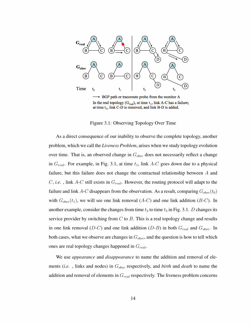
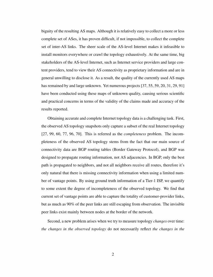
Figure 3.1: Observing Topology Over Time

As a direct consequence of our inability to observe the complete topology, another

problem, which we call the Liveness Problem, arises when we study topology evolution

over time. That is, an observed change in Gobsv does not necessarily reflect a change

in Greal. For example, in Fig. 3.1, at time t1, link A-C goes down due to a physical

failure, but this failure does not change the contractual relationship between A and

C, i.e. , link A-C still exists in Greal. However, the routing protocol will adapt to the

failure and linkA-C disappears from the observation. As a result, comparingGobsv(t0)

with Gobsv(t1), we will see one link removal (A-C) and one link addition (B-C). In

another example, consider the changes from time t2 to time t3 in Fig. 3.1. D changes its

service provider by switching from C to B. This is a real topology change and results

in one link removal (D-C) and one link addition (D-B) in both Greal and Gobsv. In

both cases, what we observe are changes inGobsv, and the question is how to tell which

ones are real topology changes happened in Greal.

We use appearance and disappearance to name the addition and removal of ele-

ments (i.e. , links and nodes) in Gobsv respectively, and birth and death to name the

addition and removal of elements in Greal respectively. The liveness problem concerns

14

how to infer the real births and deaths from observed appearances and disappearances.

More specifically, when a link or node disappears from Gobsv, is it still alive in Greal?

When a link or node appears for the very first time, has it been alive in Greal before?

Answering these questions is critical to studying topology evolution, as we need to

know when and where births and deaths occur in Greal.

The liveness problem and completeness problem are related in that solving one

will help solve the other. If the liveness of links and nodes is known, we can combine

observations made at different times to form a more complete topology estimate. For

example, in Fig. 3.1, combining Gobsv(t0) and Gobsv(t1) will give a more complete

topology at time t1, provided that we know linkA-C is still alive at time t1. Similarly, if

the complete topology is known, we will be able to differentiate real topology changes

from transient routing changes. For example, if we know the complete topology in

Fig. 3.1, we will not take the appearance of link B-C at time t1 as a birth.

However the liveness problem and completeness problem are also fundamentally

different. On the one hand, even if we know the liveness of all the observed links and

nodes over time and are able to combine observations made through a long time period,

we still do not know whether the combined topology is complete, or how incomplete

it may be. For example, in Fig. 3.1, from time t2 to time t3, knowing the liveness of

links and nodes does not help tell whether link B-C exists. On the other hand, even if

monitors are placed at every node to capture all the links (except those having failures

at the moment), when link A-C disappears from the observation at time t1, we still

cannot tell instantly whether it is due to an operational failure or the termination of

the inter-AS contract, although observations over time can provide a good estimate as

described later in this thesis.

Both the liveness problem and completeness problem are important to a full under-

standing of the Internet topology and its evolution. An ideal solution would be having

15

all the ISPs register their inter-AS connectivity at a central registry and keep their en-

tries up-to-date, which, unfortunately, does not seem feasible in the current Internet.

A near ideal solution would be placing a monitor in each AS, which is also infeasi-

ble in reality. A number of research efforts have been devoted to making Gobsv more

complete, without knowing exactly how close the obtained Gobsv is to Greal. However,

to our knowledge, no one has addressed the liveness problem, which has been a ma-

jor hurdle to empirical studies of topology evolution. In this thesis, we focus on the

liveness problem and propose a solution based on the analysis of available topology

data.

Intuitively, real topology changes generally occur over relatively long time inter-

vals (e.g. , months or even years), while transient routing changes happen within much

shorter periods (e.g. , minutes or hours). Thus if we keep observing the topology

over time, we should be able to differentiate topology changes from transient routing

changes. For example, if a link disappears and re-appears after a short period of time,

it is most likely that the disappearance is not a death. If a link disappears and never

re-appears again over a long time period, it is most likely that the link no longer ex-

ists. The research question is how long one should wait before declaring a birth or

death with a given level of confidence. We develop an empirical model that captures

the effects of long-term topology changes and short-term routing changes on observed

topologies.

Internet topology can be abstracted at different granularity, e.g. , router-level topol-

ogy, AS-level topology, and ISP-level topology (a number of ISPs have multiple ASes).

Although this thesis focuses on the AS-level topology, the liveness problem is a gen-

eral problem that exists independently from whether the nodes in Fig. 3.1 are routers,

ASes, or ISPs. Thus we believe that solving the problem at the AS-level could lead

a way to liveness solutions at other granularity. For example, if we can identify real

16

topology changes for each AS, by combining the behavior of ASes that belong to the

same ISP, we will get the topology changes for ISP-level topology. One of our future

work is to apply the methodology developed in this thesis to other types of topologies.

17

CHAPTER 4

A Solution to the Liveness Problem

In this chapter we develop a solution to the topology liveness problem based on em-

pirical data and provide some example applications of the model.

4.1 An Empirical Model of Observed Topology Dynamics

We develop the model using BGP log data, verify its consistency with information

extracted from Internet registries, and evaluate the suitability of router configuration

files and traceroute data sets in solving the liveness problem.

4.1.1 Data Sets

We use data from four different types of sources: BGP, router configurations, tracer-

oute, and Internet registries. The BGP data consists of both routing tables and updates

collected by RouteViews [15] and RIPE-RIS [14] from a few hundreds of monitors be-

tween January 1, 2004 and December 1, 2006, a period of almost three years 1. From

BGP routing tables and updates, we extract topology information (i.e. , AS nodes

and links) and record the timestamps of appearances and disappearances of links and

nodes. There are totally 27,972 nodes and 123,182 links in the entire data set. To

evaluate the effects of different monitors, we group BGP data into three sets.

1The main reason for starting from 2004 instead of earlier is to have an adequate number of monitorsfor the entire measurement period.

18

50000

100000

150000

200000

0 200 400 600 800 1000

Cum

ulat

ive

num

ber

of li

nks

obse

rved

Number of days since January 1st 2004

Tier-1Set-54

All

Figure 4.1: Number of links captured by

different sets of monitors

0

100

200

300

400

500

600

700

0 50 100 150 200 250 300

Num

ber

of p

eers

Number of covered ASes

Figure 4.2: Number of monitors in Route-

Views and RIPE-RIS combined

20000

30000

40000

50000

60000

70000

80000

90000

0 200 400 600 800 1000

Cum

ulat

ive

num

ber

of li

nks


2004-01-012004-07-012005-01-012005-07-012006-01-01

Figure 4.3: Number of links, Tier-1 moni-

tor with different starting times

30000

40000

50000

60000

70000

80000

90000

100000

110000

120000

130000

0 200 400 600 800 1000

Cum

ulat

ive

num

ber

of li

nks

obse

rved

Number of days since Jan 1st 2004

DataLinear component

Fit

Figure 4.4: Visible links seen by all moni-

tors

19

• Tier-1: data from a single monitor residing in a Tier-1 network.

• Set-54: data from a set of 54 monitors residing in 35 ASes; these monitors are

present throughout the entire measurement period.

• ALL: data from all monitors.

The traceroute data is collected and kindly provided to us by three research projects:

Skitter [17], DIMES [82], and iPlane [57]. They all have monitors around the globe to

periodically traceroute thousands of destination IP addresses, and convert router paths

to AS paths. They differ in the number of monitors, locations of monitors, probing

frequency, and the list of destinations to probe. Both Skitter and DIMES have data

from January 1, 2004 to December 1, 2006, but iPlane’s data collection only started

from late June, 2006. Each data set comes with an AS adjacency list describing the

AS topology it observes.

We also extract AS number allocation data from Regional Internet Registries (RIR) [12],

and AS connectivity information from Internet Routing Registries (IRR) [7].

In addition to the above publicly available data sources, we also made use of router

configuration data of all the routers of a Tier-1 backbone network, which includes

historical configuration files of more than one thousand routers filtered as described

in [70]. Moreover, we have access to iBGP feeds of several routers in this network.

Finally, in Section 4.3 we also use iBGP data provided by Abilene, the US research

and educational network.

4.1.2 An Empirical Model

We first use BGP data to develop an empirical model for observed topology changes.

Before starting the model development, we would like to note an important difference

between links and nodes in terms of their observability. Due to the relatively small

20

0

10000

20000

30000

40000

50000

60000

0 200 400 600 800 1000

Cum

ulat

ive

num

ber

of li

nks

Disappearance period of links

Tier-1Set-54

All

Figure 4.5: Link disappearance period

0

10000

20000

30000

40000

50000

60000

0 200 400 600 800 1000

Cum

ulat

ive

num

ber

of li

nks

Disappearance period

DataLinear component

Fit

Figure 4.6: Link disappearance period, by

all monitors

number of existing monitors and the rich connectivity among ASes, many links are

not seen on the first day of observation; some of them get revealed through routing

dynamics over time. However, because most ASes (over 99%) originate one or more

prefixes, they appear in the global routing table on the first day of observation; the

small number of remaining transit ASes behave in the same way as links in terms of

their observability. As a result, the same model applies to both links and nodes. We

will focus on developing the model for links, and only show the results of applying the

model to nodes.

4.1.2.1 The Appearance of Links and Nodes

Observations: Fig. 4.1 shows the cumulative number of unique links captured by dif-

ferent monitor sets over time. Taking the Tier-1 curve for instance: on the first day,

the observed links are those in the monitor’s routing table on January 1, 2004; a point

(200, 40000) on the curve means that during the first 200 days, this monitor has seen

40000 unique links in total from its BGP routing tables and updates.

21

As shown in Fig. 4.1, all the three curves share a common pattern: they start with

a relatively high growing rate, but slows down over time and settle on a more or less

constant growth rate. For the ALL curve, despite that the number of monitors has been

changing over time (see Fig. 4.2), its overall shape is the same as the other two’s,

except slight bumpiness at the beginning. The same pattern also holds across different

starting times of the observation, as shown in Fig. 4.3. Therefore, this pattern hints at

something fundamental to topology observation.

Intuitively, we can interpret the linear portion of the curve as due to real topology

changes (i.e. , link births) and the initial fast growth as caused by originally hidden

links being revealed by transient routing dynamics. The curves show that, within the

first 100 to 200 days, most links that could be revealed have shown up. After that

point the effect of the revelation process becomes minimal, and the curves would have

flattened out eventually had there been no link birth. The sustained linear increase of

the curves gives a strong indication of topology changes by link births. We derive an

empirical model to quantify this intuition as follows.

Modeling: According to their observability, we sort all links into three types: Visible

(links that have been observed), Invisible (links that cannot be observed by the given

set of monitors2) and Hidden (links that are possible to be observed but have not yet).

Fig. 4.1 and Fig. 4.3 show the cumulative number of unique visible links over time.

We make the following two simple assumptions:

• Constant Birth Rate: Let bv be the birth rate of visible links, bh the birth rate of

hidden links, then the total birth rate of visible and hidden links b = bv + bh.

• Uniform Revelation Probability: The probability for each hidden link to be re-

vealed during a small time interval ∆t is λ∆t.2Invisible links exist because of routing policies, e.g. , a peer-to-peer link between two ASes will

not be advertised to their providers, thus it cannot be observed by monitors in the provider networks.

22

At a given time t, let v(t) be the cumulative number of visible links observed from

time 0 to time t, and h(t) be the number of hidden links at time t. Consider a small

time interval from t to t+∆t. During this period, λ ·h(t)∆t hidden links are revealed;

at the same time, bh ·∆t new hidden links are born. Therefore,

∆h = h(t+ ∆t)− h(t) = −λh(t)∆t+ bh∆t = (bh − λh(t))∆t

∆h

bh − λh(t)= ∆t

Integrating both sides from time 0 to time t, we have:

h(t) = h0e−λt +

bhλ

(1− e−λt)

where h0 is the number of hidden links at time 0. Since h(t → ∞) = bhλ

, we can

re-write the above equation as

h(t) = h0e−λt + h∞(1− e−λt)

Now consider the number of observed links v(t), between time t and t+∆t,

∆v = λh(t)∆t+ bv∆t = λ(h0 − h∞)e−λt∆t+ b∆t

Integrating both sides from time 0 to time t, we get

v(t) = v0 + bt+ (h0 − h∞)(1− e−λt) (4.1)

where v0 is the number of links observed on the first day, bt reflects the linear birth

process, h0 is the initial number of hidden links, h∞ is the number of hidden links as

observation time t→∞, and the impact of revelation process decreases exponentially

over time.

Results: We perform non-linear regressions on the data based on Eq. 4.1, and the fit is

very good for all three sets of monitors, including the ALL curve (Fig. 4.4), which has a

23

0

50

100

150

200

250

300

350

0.2 0.3 0.4 0.5 0.6 0.7 0.8 0.9 1

Obs

erva

tion

perio

d (d

ays)

Confidence

BirthDeath

Figure 4.7: Observation period as a func-

tion of confidence level for links

0

2000

4000

6000

8000

10000

12000

0 200 400 600 800 1000

Cum

ulat

ive

num

ber

of A

Ses


RIRLinear fit (b=10.4)

Figure 4.8: Node birth from RIR

changing set of monitors over the measurement period. All regression results presented

in this thesis (e.g. , Fig. 4.4, 4.6, 4.11 and 4.14) have high coefficient of determination,

R2 > 99.5%. The good fitting indicates that the simple model approximates real data

satisfactorily. As explained earlier, the same model should apply to nodes as well,

since hidden nodes are revealed in the same way as hidden links by routing dynamics.

The fit to node data is also very good. Values of model parameters are obtained from

regressions and listed in Fig. 4.1.

Through further examinations of the inter-AS relations, we also developed the

following observations. First, the hidden AS links correspond to backup customer-

provider links which are revealed over time. Second, there should be no hidden peer

links, because, generally speaking, peer links are always used to carry routes. They

are used in primary rather than backup routes, thus peer links are immediately visible

unless they are invisible. Furthermore, the truly invisible links correspond to peer links

between lower tier ASes which do not have monitors installed. That is, the invisible

links are under the line of sight of all the existing monitors. [70] presents addtional

elaborations on these observations.

24

Parameters Links Nodes

Birth rate b (day−1) 67.3 10.3

Revelation λ (day−1) 0.0151 0.0223

(h0 − h∞) 11013 240

Death rate d (day−1) 45.7 2.87

Revelation µ (day−1) 0.0196 0.0172

f0/µ 10545 797

Table 4.1: Model Parameters

4.1.2.2 The Disappearance of Links and Nodes

Observations: A link disappeared from Gobsv(t) can be a real death, or it can be still

alive inGreal, not observed by any monitor at the moment but may re-appear sometime

in the future. Assuming the observation period ends on day n, we define that a link has

a disappearance period of (n−m) days if the link disappeared on day m and has not

re-appeared until the end of the observation. Note that even though a link may appear

and disappear many times in the entire observation period, only the last disappearance

counts in calculating the link’s disappearance period.

Fig. 4.5 shows the cumulative number of links over the disappearance period. For

instance, a data point at (200, 21000) on the Tier-1 curve means that, at the end of the

observation, 21000 links have a disappearance period less than or equal to 200 days

as seen by the Tier-1 monitor. Interestingly, the curve also exhibits the pattern of an

initial exponential component plus a stable linear component over time, and this same

pattern holds across different monitor sets and different observation ending times.

Modeling: We divide visible links into two subtypes: in-sight (links that are in the

25

currently observed topology Gobsv(t)), and out-of-sight (links that have been seen pre-

viously, but are not inGobsv(t), and may come back toGobsv sometime later). We make

two simple assumptions:

• Constant Death Rate: In-sight links disappear from the monitors’ view at a rate

of d + f0, where d is the number of link deaths, f0 the number of links that

become out-of-sight, per unit time.

• Uniform Revelation Probability: For each out-of-sight link, the probability of

being revealed (i.e. , become in-sight again) during a small time interval ∆t

is µ∆t. This revelation process is essentially the same as the one described

earlier for appearance. We use different notations, λ and µ, since the former is

computed from the first appearance of links, and the latter is computed from the

re-appearance of links.

Suppose the observation ends at time tend. Consider the f0 links that become out-

of-sight at time td, and s = tend − td. Let f(x) be the number of these links that have

not re-appeared since time td through time td + x. After a short time period ∆x, some

of these links may be revealed by routing dynamics. Therefore,

∆f(x) = f(x+∆x)− f(x) = −µf(x)∆x

Integrating from x = 0 to x = s,

f(s) = f0e−µs

At the end of observation, the number of links with disappearance period of s is equal

to d + f(s). Let z(s) be the cumulative number of links whose disappearance period

is less than or equal to s, then

z(s) =

∫ y=s

y=0

(d+ f(y)) dy =f0

µ(1− e−µs) + sd (4.2)

26

0

5000

10000

15000

20000

25000

30000

35000

40000

0 100 200 300 400 500 600

Cum

ulat

ive

num

ber

of n

ew li

nks

obse

rved

Number of days since April 5th 2005

IRR dataLinear fit: b=57.6

Figure 4.9: Link birth from IRR

0

2000

4000

6000

8000

10000

12000

0 100 200 300 400 500 600

Cum

ulat

ive

num

ber

of li

nks

Disappearance period (days)

IRR dataLinear fit: d=18.6

Figure 4.10: Link death from IRR

where the death process is captured by a linear term, and the revelation process (of

disappeared links) is captured by an exponential term.

Results: Eq. 4.2 fits data well and the results are shown in Fig. 4.6. The same model

can also be applied to nodes. Model parameters, for both appearance and disappear-

ance of links and nodes, are listed in Fig. 4.1. Even though λ is estimated from first

appearance and µ is estimated from re-appearance, they have similar numerical values,

which is consistent with our model that both parameters characterize the same revela-

tion process. Note that in deriving the model for link appearance, we did not take into

account the death process of visible or hidden links for clarity. The death of visible

links does not affect Eq. 4.1 because Eq. 4.1 is about cumulative number of observed

links. Assuming the death rate for hidden links is dh, the only change it makes in

Eq. 4.1 is to replace bh by (bh − dh), e.g. , b = bv + bh − dh instead of bv + bh.

4.1.2.3 Distinguishing Topology Changes from Transient Routing Changes

Based on our empirical model, the effects of transient routing dynamics on observed

topology decrease exponentially over time, while the real birth and death occur at

constant rates. If one observes the topology long enough, the observed changes will

27

0

10000

20000

30000

40000

50000

60000

70000

80000

90000

0 200 400 600 800 1000

Cum

ulat

ive

num

ber

of li

nks

obse

rved


EmpiricalLinear component

Fit

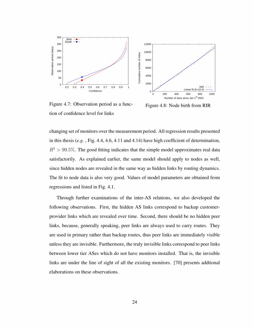
Figure 4.11: Visible links in Skitter, λ = 0.00598, b = 39.86.

be dominated by real topology changes. Assume the observation starts at time tstart,

ideally one can wait for a sufficiently long time B so that every new link appearance

at time t > tstart + B can be considered a birth with high confidence. Similarly, after

a link disappears, one can wait for a sufficiently long time D and if the link does not

re-appear during this time, it can be considered a death with high confidence. Now we

are ready to quantify B and D with certain confidence.

According to our model, on each day the newly discovered links come from two

sources: bv from birth and λh(t) from revelation. If we count all the newly discovered

links on day t as birth, the chance of being correct is

confidence(t) =bv

bv + λh(t)=

bvb+ λ(h0 − h∞)e−λt

(4.3)

From regression on data, we can obtain the values of b, λ, and (h0−h∞). To estimate

bv, we assume bv ' b. This is based on the following observation. Since b = bv +

bh − dh, our assumption is equivalent to bh ' dh. If bh and dh differ significantly,

the number of hidden links at the beginning of observation would vary significantly

with different starting dates, i.e. , h0 as well as (h0 − h∞) would change significantly

over different starting dates. However, our examination of data shows that this is not

28

the case, i.e. , (h0 − h∞) remains relatively stable over different starting dates, which

validates the assumption of bh ' dh and bv ' b.

Knowing the values of the parameters, we can now calculate B for a given confi-

dence level using Eq. 4.3. Similarly, D can be calculated for a given confidence level

based on our model of disappearance. Fig. 4.7 shows the values of B and D for dif-

ferent confidence values. For instance, after 205 days from January 1, 2004, we can

count all newly discovered links as real births with 90% or higher probability of being

correct. If a link disappears and does not show up after 189 days, with 90% chance

this is a real death.

So far we have considered links and nodes separately. For a given observation

period (B or D), the confidence level of nodes usually is higher than that of links.

Thus considering both together sometimes can improve the confidence on links. For

instance, a node birth is always accompanied by some link births. Therefore we can

decide these link births with higher confidence than what we would have by only con-

sidering links.

4.1.3 Comparison with router configuration files from a Tier-1

In this section we compare the connectivity of a Tier-1 network extracted from Route-

views and RIPE-RIS since early 2004 (“BGP data”) with the connectivity obtained

from router configuration files as described in [70]. This process involves collecting

all router configuration files from the Tier-1 network and process them to extract AS

adjacencies. To reduce the number of false positives, we only consider BGP sessions

for which there is a valid route configured between the two incident routers. Fur-

thermore, we remove BGP sessions for which there are no syslog messages since a

reasonable long time (the process is explained in more detail in [70]). As a first step

we compare the appearance rate of incident links to the Tier-1 as observed from BGP

29

data and as extracted from router configs, which is shown in Figure 4.12. We note

that the curves are very close to each other (the top curve has only ∼ 7% additional

slope), and the gap is solely caused by neighbors that announce prefixes that are longer

than /24, which are aggregated in a shorter prefix originated by the Tier-1. These links

never appear in eBGP, even though they are revealed in iBGP routes inside the Tier-1.

Figure 4.13 shows the difference between the appearance timestamps of incident AS

links of the Tier-1 as seen in BGP data from RouteViews and RIPE (birthBGP ) and

from router configs (birthcon). We observe that almost 80% of the AS links appear in

router configs in the same day as they appear in BGP. The remaining 20% have some

lag between the time they appear in the configs and the time they appear in BGP, which

can be on the order of several months. This is expected since the router configs in this

study are only from one side of the BGP session, i.e. the neighbor AS may take more

time to configure the session on their routers. The fact that we were using a monitor

of the Tier-1 network in the BGP view contributes to the high accuracy of the link

appearance timestamps, since direct links to the monitor are preferred in BGP routes,

and hence immediately revealed (versus being hidden).

0

0.1

0.2

0.3

0.4

0.5

0.6

0.7

0.8

0.9

1

0 100 200 300 400 500 600

Cum

ulat

ive

num

ber

of li

nks

(nor

mal

ized

)


router configsBGP data

Figure 4.12: Comparison between routers’

config files connectivity and BGP data

(cumulative) from a Tier-1 network.

0

0.1

0.2

0.3

0.4

0.5

0.6

0.7

0.8

0.9

1

0 20 40 60 80 100

Num

ber

of li

nks

(CD

F)

birthBGP-birthcon (days)

Figure 4.13: Comparison of appearance

times between routers’ config files and

BGP data of a Tier-1 network.

30

0

10000

20000

30000

40000

50000

60000

70000

0 200 400 600 800 1000

Cum

ulat

ive

num

ber

of li

nks

Disapperance period

EmpiricalLinear component

Fit

Figure 4.14: Link disappearance period,

by Skitter, µ = 0.0385, d = 57.61.

0

0.1

0.2

0.3

0.4

0.5

0.6

0.7

0.8

0.9

1

-1000 -500 0 500 1000

CD

F

Bsk - Bbgp (days)

Figure 4.15: Comparison of appearance

timestamps between Skitter and BGP.

4.1.4 Comparison with Internet Registry Data

Our model is built upon the assumption that a linear term captures real topology

changes in Greal. Here we use Internet registry data to check the soundness of this

assumption. The registry data is particularly useful because it is not affected by rout-

ing dynamics.

Regional Internet Registries (RIRs) [12] maintain complete history of AS number

allocations. Fig. 4.8 shows the cumulative number of allocations since January 1, 2004.

It can be approximated by a straight line with slope of 10.4 nodes/day, very close to

10.3 nodes/day obtained from our model 3. Since there is a variable delay between an

AS number’s allocation and its announcement in the global routing system, we cannot

use the allocation date to verify the birth date of nodes. However, the fact that the

AS allocation exhibits a growth rate extremely close to that derived from our model

provides a supporting evidence for our assumption of linear node birth. We are not

3Some AS numbers are allocated but never used for global routing. The cumulative number of suchASes grows over time, which may explain the slight difference between node birth rates obtained fromRIR and BGP data.

31

able to check node death rate with RIR data since deallocation of AS numbers is not

mandated and usually is not done in practice.

Internet Routing Registries (IRR) [7] are databases for registering inter-AS con-

nections and routing policies. Registration with IRR is done voluntarily. It is known

that information in IRR is incomplete, and out-of-date for some entries. Historic IRR

files are not publicly available, but we have been downloading a daily copy since April

5, 2005. Fig. 4.9 shows link appearances and Fig. 4.10 shows link disappearances

based on IRR data. Again, one cannot use the IRR data to verify the birth/death dates

of individual links, since registering a link and bringing a link up usually happen on

different days. Both figures exhibit linear behavior over time, which is consistent with

our assumption of linear link birth and death. The rates obtained from IRR data are

lower than that from BGP data, which is likely due to the incompleteness of IRR data.

More specifically, the birth rate estimated in Fig. 4.9 is about 86% of that from BGP

data, whereas the death rate estimated in Figure 4.10 is only 40% of that from BGP

data. This indicates that even some operators are willing to register their connectivity,

they still tend to overlook the removal of stale information.

4.1.5 Evaluation of Traceroute Data

Besides BGP routing tables and updates, traceroute data is another major source for

AS topology information. In this subsection, we analyze existing traceroute data with

regard to their effectiveness in solving the liveness problem.

4.1.5.1 Measuring AS Topology by Traceroute

BGP and traceroute measurements work differently. A BGP data collector passively

listens to routing updates regarding all the globally announced IP prefixes from indi-

vidual monitors and logs the updates as well as routing tables for each monitor. A

32

0

0.1

0.2

0.3

0.4

0.5

0.6

0.7

0.8

0.9

1

-1000 -500 0 500 1000

CD

F

Dsk - Dbgp (days)

Figure 4.16: Comparison of disappear-

ance timestamps between Skitter and

BGP.

350000

400000

450000

500000

550000

600000

650000

700000

750000

2004 2005 2006 2007

Num

ber

of r

each

able

add

ress

es

Time

Figure 4.17: Number of reachable ad-

dresses in Skitter destination list.

traceroute monitor actively sends UDP or ICMP probes to a list of IP addresses and

records the router-level paths, which is then converted to AS-level paths.

BGP and traceroute data can be complementary in topology measurement. Since

usually their monitors are placed in very different locations, they may be able to see

different parts of the Internet topology. Also, BGP data records the routing paths, while

traceroute records the data paths, which can be different in some cases. For example,

if a provider AS P aggregates a customer AS C’s prefix in P ’s routing announcement,

a BGP monitor may not be able to see the link P -C, but traceroute can reveal its

existence. However, as pointed out in [64, 44, 28], accurately converting router paths

to AS paths remains an open issue, and there can be many pitfalls in this process.

One commonly used method of converting router IP addresses to AS numbers is to

look up BGP routing table and RIR address allocation database, which, as shown in

previous work, may introduce false AS links. For example, assuming three ASes are

connected asA-B-C, ifB’s border router uses one ofA’s IP addresses, then the simple

conversion will give a false AS link A-C.

33

As a sanity check on traceroute data, we compared the links observed in BGP data

with that reported by Skitter during January 2007, and manually verified the differ-

ence between the two data sets by contacting the operators of 20 ASes. For these 20

ASes, Skitter reported 447 links that were not in BGP data. However, only 16 out

of these 447 links (4%) were confirmed by the operators. Unfortunately, all the three

major traceroute data sets mentioned later in this section used BGP tables and WHOIS

lookups for the IP address to AS number conversion, thus they may potentially suffer

the same conversion errors4. Due to the potentially false links in the data sets, we did

not include traceroute data in our model development. However, since traceroute data

potentially can be a very valuable source for AS topology information, we evaluate the

three data sets and discuss the impact of two important measurement factors: probing

frequency and destination list.

4.1.5.2 Skitter

During our measurement period, Skitter has about 20 monitors around the globe. Ev-

ery day each monitor probes every IP address in a fixed list of around 970,000 ad-

dresses [18]. We apply our model to Skitter data. Fig. 4.11 shows the cumulative

number of unique links observed, and Fig. 4.14 shows the disappearance period of

links. The curves have the same shape as BGP data and our model fits the data well,

which means that the model can be applied to the topology dynamics observed by

traceroute too. However, the observed parameters may not reflect the real rates of birth

and death due to the data set’s limitations.

First, Skitter’s revelation parameters are different from that obtained from BGP data.

Its λ is less than the half of BGP’s, and its µ is about twice as BGP’s. These differences

can be explained as follows. When a routing change happens, a BGP monitor will be

4iPlane improves the conversion by first doing alias resolution of IP addresses and then mappingeach IP address to the AS that majority of the addresses in the alias map to.

34

notified by triggered routing updates. But for a traceroute monitor to see the change, it

must probe the path when the change is still in effect. For instance, if a hidden backup

link is exposed for 2 hours and the monitor probes once every 24 hours, the chance to

discover this link is only 2/24 = 8%. Since primary paths (links) are being used in the

majority of time, and Skitter only probes each destination once every day, the chance

of observing backup paths (links) is small. Therefore, Skitter is slow in discovering

backup links (i.e. , small λ), but quick in picking up recovered primary links (i.e. ,

large µ). This is further verified by examining the links observed by both BGP and

Skitter. Fig. 4.15 shows the difference between BGP’s and Skitter’s timestamps for the

same link, when they discover the link for the first time. BGP discovers 60% of links

earlier than Skitter, Skitter discovers 10% of links earlier than BGP, and they discover

30% of links on the same day. Fig. 4.16 shows the difference between BGP’s and

Skitter’s timestamps when they see a particular link for the last time. BGP observes

50% of links for longer time, Skitter observes 10% of links for longer time, and they

see 40% of links on the same day for the last time. Clearly, to be more effective in

observing topology dynamics, traceroute data collection needs to probe destinations

frequently5.

Second, Skitter data shows a higher death rate (57.61/day) than the birth rate

(39.86/day), which implies that the observed topology shrinks every day, and we have

verified it by counting the number of unique nodes and links observed by Skitter ev-

eryday. This is a result of Skitter using a fixed list of destination IP addresses over

several years. Using a fixed destination list underestimates the birth rate because new

ASes (which announce new prefixes) and their links will not be probed. It also over-

estimates the death rate because over time some IP addresses on the fixed list become

unreachable due to various reasons. For example, a noticeable percentage of prefixes

stop being announced over time [66], or an ISP may decide to block ICMP traffic.

5High probing frequency may cause security concerns from networks being probed.

35

Fig. 4.17 clearly shows the decline of reachable addresses in Skitter’s destination list.

Many links that Skitter no longer observes are due to its shrinking probing scope, not

because the links are dead. To be effective in observing topology dynamics, traceroute

data collections must update the destination list constantly to include all ASes.

4.1.5.3 DIMES

DIMES [82] is a distributed measurement infrastructure consisting of a large num-

ber of agents installed by end users on their computers. These agents periodically

traceroute or ping a given set of destinations. The number of DIMES agents has been

growing rapidly, from a few hundreds in early 2005 to almost 12,000 in late 2006.

Each DIMES agent probes a different destination list, which is computed and updated

periodically [82]. The probing frequency varies for different agents, and can be as

low as once per week. The purpose of using partial destination lists and low probing

frequency for each agent is to distribute the measurement load among agents while

maintaining a good coverage of the topology. Fig. 4.26 shows the cumulative number

of links observed by DIMES over time. Although its overall trend is similar to BGP’s

and Skitter’s, the curve is much more irregular due to the fast growth of DIMES agents,

partial and changing destination lists, and different probing frequencies.

4.1.5.4 iPlane

iPlane [57] employs around 200 monitors installed on PlanetLab nodes [33]. All iPlane

monitors use a common destination list extracted from BGP routing tables daily, and

probe one address inside every /24 address block. The destinations are being probed

once every day by every monitor. iPlane’s measurement scheme seems very promising

in terms of observing topology dynamics. However, its starting date is recent (June

2006), whereas the BGP data set goes back to 2004.

36

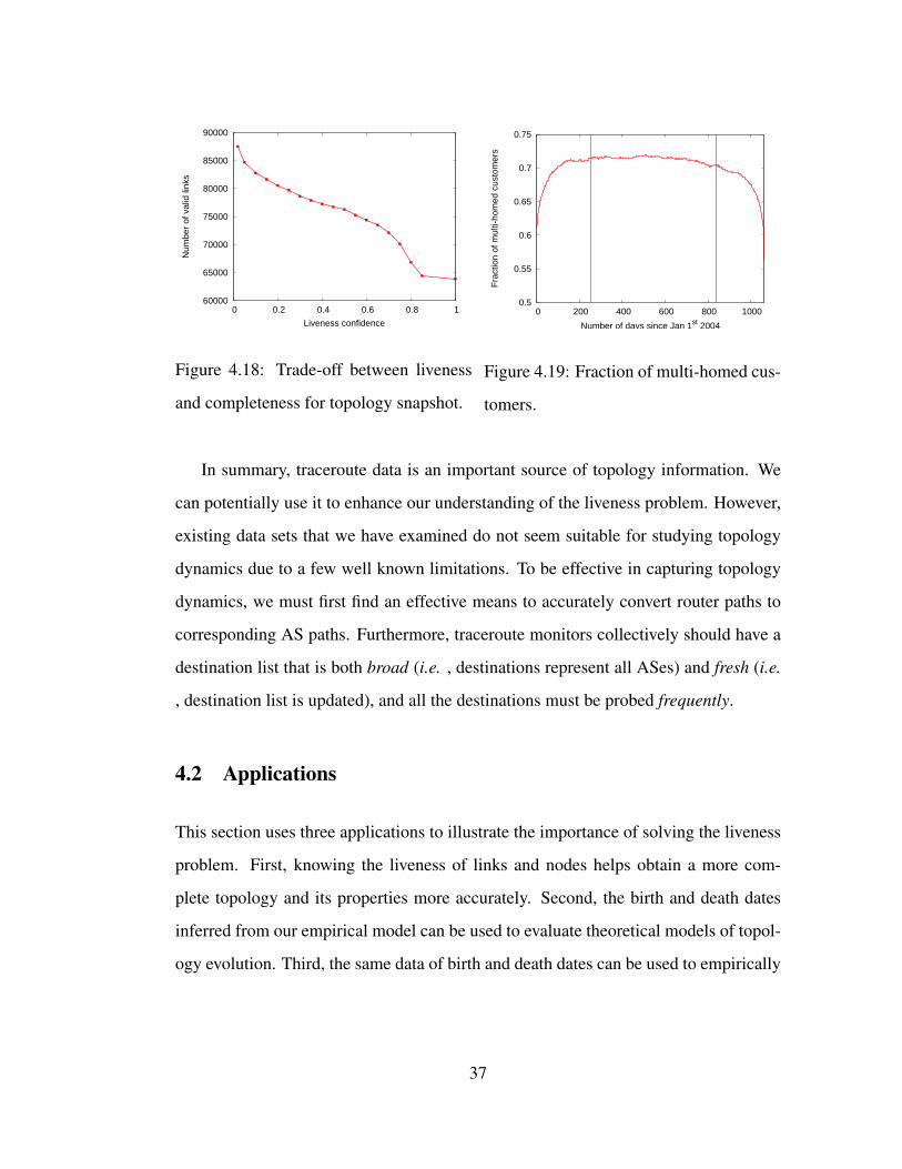
60000

65000

70000

75000

80000

85000

90000

0 0.2 0.4 0.6 0.8 1

Num

ber

of v

alid

link

s

Liveness confidence

Figure 4.18: Trade-off between liveness

and completeness for topology snapshot.

0.5

0.55

0.6

0.65

0.7

0.75

0 200 400 600 800 1000

Fra

ctio

n of

mul

ti-ho

med

cus

tom

ers


Figure 4.19: Fraction of multi-homed cus-

tomers.

In summary, traceroute data is an important source of topology information. We

can potentially use it to enhance our understanding of the liveness problem. However,

existing data sets that we have examined do not seem suitable for studying topology

dynamics due to a few well known limitations. To be effective in capturing topology

dynamics, we must first find an effective means to accurately convert router paths to

corresponding AS paths. Furthermore, traceroute monitors collectively should have a

destination list that is both broad (i.e. , destinations represent all ASes) and fresh (i.e.

, destination list is updated), and all the destinations must be probed frequently.

4.2 Applications

This section uses three applications to illustrate the importance of solving the liveness

problem. First, knowing the liveness of links and nodes helps obtain a more com-

plete topology and its properties more accurately. Second, the birth and death dates

inferred from our empirical model can be used to evaluate theoretical models of topol-

ogy evolution. Third, the same data of birth and death dates can be used to empirically

37

0

0.02

0.04

0.06

0.08

0.1

0.12

1 10 100 1000

Atta

chm

ent p

roba

bilit

y

Target node degree

Figure 4.20: Attachment probability distribution for a target node degree.

characterize topology growth trends. Although these applications demonstrate the use-

fulness of our model, the accuracy of the numerical results may be affected by the raw

data available. Recent work [96, 70] point out that this topology may miss a significant

number of peer-to-peer links6.

4.2.1 More Accurate View of the Topology

The AS topology on a particular day is often referred to as a topology snapshot. Un-

derstanding the graph properties of a topology snapshot (static view) and the changes

of the properties over time (dynamic view) is an active research area. Knowing the

liveness of links and nodes can help capture more accurate views of the topology.

6The topology in [96] is collected from BGP routing tables, IRR, and traceroute data. Our topologyis collected from both BGP routing tables and routing updates. A comparison of the two topology datasets on May 12, 2005 shows that our set has 9154 additional links but misses 7056 links.

38

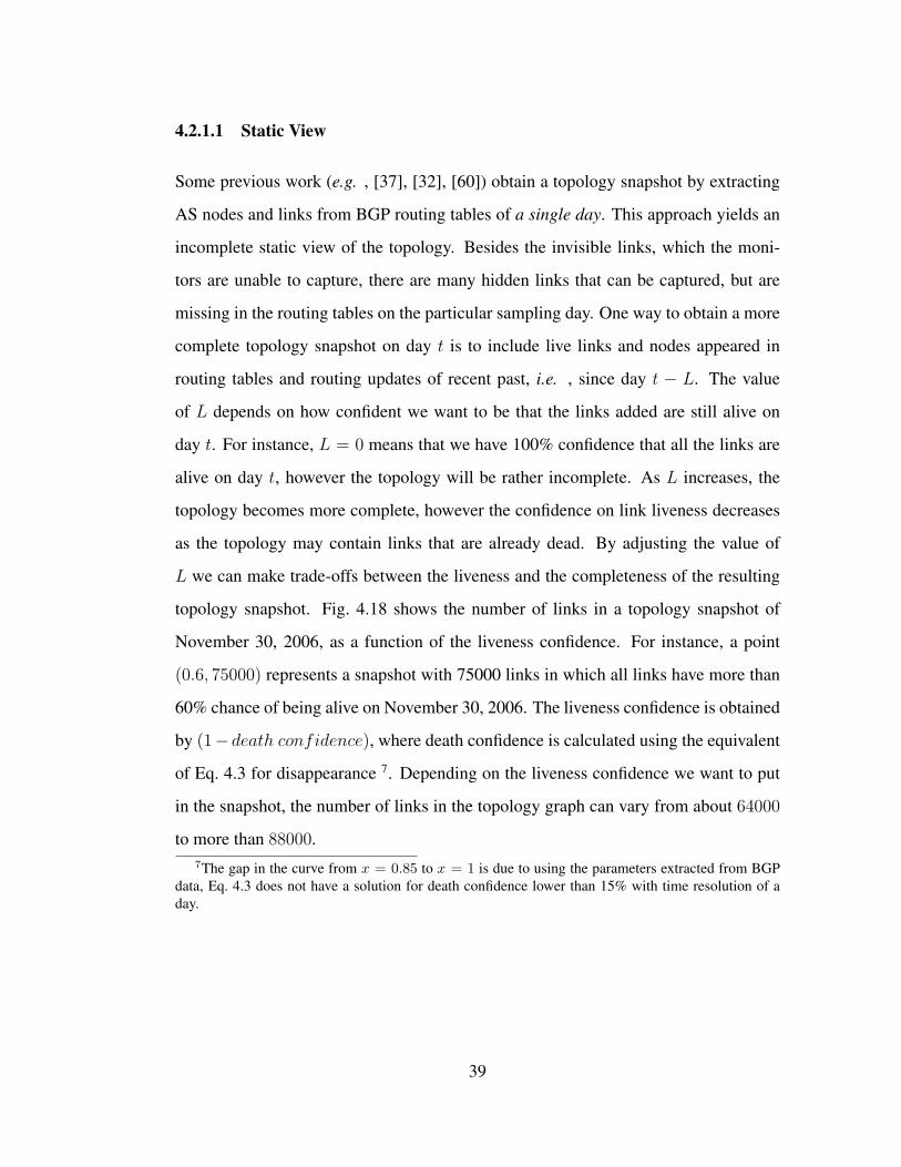
4.2.1.1 Static View

Some previous work (e.g. , [37], [32], [60]) obtain a topology snapshot by extracting

AS nodes and links from BGP routing tables of a single day. This approach yields an

incomplete static view of the topology. Besides the invisible links, which the moni-

tors are unable to capture, there are many hidden links that can be captured, but are

missing in the routing tables on the particular sampling day. One way to obtain a more

complete topology snapshot on day t is to include live links and nodes appeared in

routing tables and routing updates of recent past, i.e. , since day t − L. The value

of L depends on how confident we want to be that the links added are still alive on

day t. For instance, L = 0 means that we have 100% confidence that all the links are

alive on day t, however the topology will be rather incomplete. As L increases, the

topology becomes more complete, however the confidence on link liveness decreases

as the topology may contain links that are already dead. By adjusting the value of

L we can make trade-offs between the liveness and the completeness of the resulting

topology snapshot. Fig. 4.18 shows the number of links in a topology snapshot of

November 30, 2006, as a function of the liveness confidence. For instance, a point

(0.6, 75000) represents a snapshot with 75000 links in which all links have more than

60% chance of being alive on November 30, 2006. The liveness confidence is obtained

by (1− death confidence), where death confidence is calculated using the equivalent

of Eq. 4.3 for disappearance 7. Depending on the liveness confidence we want to put

in the snapshot, the number of links in the topology graph can vary from about 64000

to more than 88000.7The gap in the curve from x = 0.85 to x = 1 is due to using the parameters extracted from BGP

data, Eq. 4.3 does not have a solution for death confidence lower than 15% with time resolution of aday.

39

4.2.1.2 Dynamic View

In order to study how graph properties of the topology change over time, the effects

of revelation process on the observed topology must be taken into consideration. As

an example, assume we want to measure the percentage of multi-homed stub ASes

over time. A stub AS is the one that always appears as the last AS in an AS path; it

corresponds to a customer network at the bottom tier of the Internet routing hierarchy.

A stub AS may connect to multiple network service providers, but it does not forward

data traffic between its providers. Fig. 4.19 shows the percentage of multi-homed

stub ASes without considering the effects of revelation process: starting with an initial

snapshot on the first day, the topology is updated every day by adding links as they first

appear and removing links according to their last-seen time, and the percentage of stub

ASes is calculated and plotted for each day’s topology. The curve shows a fast increase

at the beginning of the study period and a fast decrease at the end, which might look

puzzling at first, but can be easily explained by the revelation process. At the begin-

ning, there are many hidden links that take some time to appear, and as they appear,

we discover that existing single-homed stub ASes are in fact multi-homed. Near the

end, many in-sight links become out-of-sight, and are prematurely discounted from the

topology graph, resulting in false classification of multi-homed stub ASes into single-

homed. To take into account the effects of revelation process, in Fig. 4.19 we draw two

vertical lines corresponding to the 95% confidence margins calculated from Eq. 4.3.

Only the part of the curve between these two vertical lines reflects the real percentage

of multi-homed stub ASes with a high confidence level. This example illustrates the

importance and usefulness of our revelation model in topology measurement and other

similar types of topological studies.

40

0.2

0.3

0.4

0.5

0.6

0.7

0.8

300 400 500 600 700 800

Fra

ctio

n of

targ

et A

Ses

with

deg

ree>

d med

Number of days after January 1st 2004

Data (GLP)Data (BA)

Model median

Figure 4.21: Model evaluation

0

2000

4000

6000

8000

10000

12000

14000

16000

18000

0 200 400 600 800 1000

Net

gro

wth

of n

odes


StubTransit

Figure 4.22: Node net growth

(per day) Transit Stub Total

Node Birth 2.4 8.3 10.7

Node Death 0.8 2.5 3.3

Net Growth 1.6 5.8 7.4

Link Birth 37.7 29.2 66.9

Link Death 29.0 16.7 45.7

Net Growth 8.7 12.5 21.2

Table 4.2: Comparison Between Stub and Transit changes.

41

4.2.2 Evaluating Theoretical Models

A number of theoretical models have been proposed for network topology evolution.

They generally model the decision process of where to add/remove new links and

nodes into/from the topology at each time. A common evaluation method of these

models is to let the network grow to a certain size by simulating the link/node addi-

tion and removal processes, then compare graph properties of the resulting network

topology with that of an observed topology of a similar size. This approach to evalua-

tion, however, is limited in its effectiveness because different evolution processes can

generate topologies that share certain graph properties. A much better approach is to

compare the decisions of the theoretical models directly with the observed link/node

births and deaths, which is made possible once the liveness problem is solved. In this

section, we demonstrate the value of this new approach by applying it to evaluate two

theoretical models.

Barabasi et al. [23] proposed an evolution model (the BA model) that explains

the emergence of the power-law distribution of node degrees in complex networks.

One of the key elements in this model is the preferential attachment or rich-get-richer

paradigm. The basic idea is that new nodes tend to connect to existing nodes that

already have high degrees. More precisely, according to the BA model, a new node

attaches to an existing node i at time t with the probability pi(t) = di(t)/∑

j dj(t),

where di(t) is the degree of node i at time t, and the summation is over all the existing

nodes in the topology. Thus, the probability that a new node attaches to a node with

degree d at time t is

P (d, t) = N(d, t) · d∑j dj(t)

where N(d, t) is the number of existing nodes with degree d at time t. Fig. 4.20

shows the distribution of P (d, t) on a particular day from BGP data, and the vertical

line at dmed = 49 represents the median of the distribution. Since the distribution of

42

node degrees is heavy-tailed, i.e. , there exists a small number of nodes with high

degrees and a large number of nodes with small degrees, on average a new node has

a higher chance to attach to a small degree node than attaching to a high degree node.

To evaluate the BA model, we extract the birth and death events of links and nodes

from BGP data using 90% confidence margins provided by our model. In other words,

we record a topological change only when we are at least 90% sure that it is a real

topological change. Appearances and disappearances near the beginning and the end

of the study period are discarded to eliminate the effect of revelation process. One

main problem in evaluating a probabilistic theoretical model is that, on the one hand,

we need a large number of node births to make a meaningful sample set; on the other

hand, the degree distribution changes over time as nodes join the topology, therefore

each sample of node degrees is only good for a specific instance in time. To overcome

this problem, we use the following evaluation scheme inspired by the Monte Carlo

method: (1) Compute the distribution P (d, t) for day t and its median dmed(t). (2) For

each node born on day t + 1, check if the node it connects to has a degree higher or

lower than dmed(t); if it is higher, increment counter h, otherwise increment counter l.

(3) Repeat for every day. By the law of large numbers, if the node-join process follows

the BA model, the ratio h/(h+ l) should converge to 50%.

Fig. 4.21 plots the value of h/(h + l) over time and shows that the BA model

actually converges to 58% in the long run. This indicates that, during the evolution of

Internet AS topology, high degree nodes attracted more new nodes than what the BA

model describes. This result is also consistent with the conclusion in [32], which used

an earlier data set and different evaluation techniques.

Bu et al. [24] proposed the Generalized Linear Preference (GLP) model, in which

the probability that a new node attaches to a node with degree d is given by:

P (d, t) = N(d, t) · d− β∑j (dj(t)− β)

43

0

10000

20000

30000

40000

50000

60000

0 200 400 600 800 1000

Net

gro

wth

of l

inks


StubTransit

Figure 4.23: Link net growth

0

500

1000

1500

2000

2500

3000

3500

4000

4500

200 300 400 500 600 700 800 900

Net

gro

wth

of w

iring

s


stubtransit

Figure 4.24: Net growth of node wirings.

where β ' 0.8. Fig. 4.21 plots the result of applying our technique to the GLP model.

Note that Fig. 4.21 only checks for the median of the P (d, t) distribution, and it shows

that GLP model matches the median of the empirical data for node attachment. To

further evaluate the model, we need to compare other percentiles of the distribution as

well.

4.2.3 Characterizing Evolution Trends

We use the same data of link/node births and deaths to empirically characterize the

trends of topology evolution. Generally speaking, ASes can be classified into two

categories: stub and transit. A stub AS only appears as the last AS in an AS path,

while a transit AS will appear in the middle of some AS paths. A stub AS corresponds

to a customer network, which does not forward traffic between its neighbors. A transit

AS corresponds to a network service provider, which provides data delivery service

for other networks. In the context of the AS topology graph, we refer to them as stub

nodes and transit nodes, respectively. Links between transit nodes are called transit

44

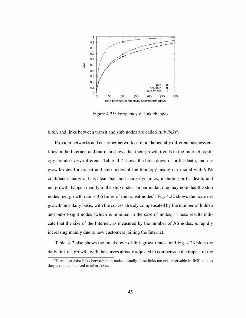
0

0.1

0.2

0.3

0.4

0.5

0.6

0.7

0.8

0.9

1

0 50 100 150 200 250 300

CD

F

Time between connectivity adjustments (days)

p2pc2p stub

c2p transit

Figure 4.25: Frequency of link changes

links, and links between transit and stub nodes are called stub links8.

Provider networks and customer networks are fundamentally different business en-

tities in the Internet, and our data shows that their growth trends in the Internet topol-

ogy are also very different. Table 4.2 shows the breakdown of birth, death, and net

growth rates for transit and stub nodes of the topology, using our model with 90%

confidence margin. It is clear that most node dynamics, including birth, death, and

net growth, happen mainly to the stub nodes. In particular, one may note that the stub

nodes’ net growth rate is 3.6 times of the transit nodes’. Fig. 4.22 shows the node net

growth on a daily basis, with the curves already compensated by the number of hidden

and out-of-sight nodes (which is minimal in the case of nodes). These results indi-

cate that the size of the Internet, as measured by the number of AS nodes, is rapidly

increasing mainly due to new customers joining the Internet.

Table 4.2 also shows the breakdown of link growth rates, and Fig. 4.23 plots the

daily link net growth, with the curves already adjusted to compensate the impact of the

8There also exist links between stub nodes, usually these links are not observable in BGP data asthey are not announced to other ASes.

45

hidden and out-of-sight links. Although the transit nodes only make about 28% of the

total nodes and their percentage is decreasing, their link birth rate is 29% higher than

that of stub links, and the death rate 74% higher. Note that the link birth and death

counts lump together all the link changes that can be either due to node birth/death

or due to link adjustment between existing nodes. To quantify the latter, we define

wiring as the addition of a new link between two existing nodes, and unwiring as the

removal of a link between two live nodes (i.e. , the two incident nodes are still alive in

the topology after the link is removed). Stub wirings and unwirings reflect customer’s

actions of changing providers, while transit wirings and unwirings reflect provider’s

actions of adjusting their inter-ISP connectivity.

Fig. 4.24 shows the net growth of wirings between July 24, 2004 and May 25, 2006,

a period that falls within our 90% confidence margins. Here we consider only the nodes

that are present throughout this measurement period and find 10349 such stub nodes

and 6319 transit nodes. We then count the wiring and unwiring events among these

nodes. Fig. 4.24 shows that provider networks get more densely connected over time,

perhaps as a result of serving ever increasing customer demands9. Keeping in mind

that the number of transit nodes is much lower than the number of stub nodes, and that

a transit wiring event means adding a link between two transit nodes only, we see a

high net growth rate in transit links, despite the high death rate shown in Table. 4.2.

This confirms a general observation that over recent years, provider networks have

been actively adjusting their inter-connectivity.

What types of inter-ISP connectivity that providers are actively adjusting? Based

on the type of inter-AS business relationships, links are generally classified into three

classes: customer-to-provider (c2p), peer-to-peer (p2p), and sibling-to-sibling (e.g. ,

ASes that belong to the same company). Since the sibling relationship is relatively

9Other relevant factors, such as increases in link capacity and the number of BGP sessions betweenneighboring ASes, are not observable in BGP data.

46

rare, here we focus on c2p and p2p links only. In c2p relationship, the customer (or

lower-tier ISP) pays its provider (or upper-tier ISP) to gain the global reachability.

In p2p relationship, data traffic is exchanged free of charge between the two peers,

but only traffic originated from a peer AS (or its customers) is allowed on this link.

We applied the PTE algorithm [39] to infer AS link relationships, and the algorithm

was able to infer the relationships for 75% of all the links involved in wirings and

unwirings. We classify wiring and unwiring events according to their link types. For

each type, we calculate the time interval between two consecutive events and plot the

distribution of the intervals in Fig. 4.25. We can see that, among c2p links, stub links

are more stable compared to c2p transit links, and that the p2p links have much shorter

intervals between their connectivity adjustments than all c2p links. According to [88],

a common ISP operational practice is to set up a p2p link and re-evaluate it periodically

(e.g. , once every few months). Based on whether the p2p link helps reduce the overall

cost, it may be either kept or terminated.

4.3 Discussion

Our model captures the main characteristics of observed AS topology changes by three

dynamic processes: birth, death, and revelation. This model can help us obtain key

parameters of different dynamic processes and separate real topology changes from

transient routing changes with a given confidence. At the same time, we must also

understand the limitations of this model.

The model is mainly descriptive and not derived from first principles. It matches

the data well and is useful in studying topology dynamics. However, it is possible to

have other models that also fit the data well, e.g. , node birth may be modeled by an

exponential function with a small exponent [43]. Our model does not provide an expla-

nation for why birth and death rates are constant, or why the revelation probability are

47

0

20000

40000

60000

80000

100000

120000

0 100 200 300 400 500 600 700 800

Cum

ulat

ive

num

ber

of li

nks

(CD

F)

Number of days since Sept 23th 2004

Figure 4.26: Number of collected links in

DIMES.

0.02

0.025

0.03

0.035

0.04

0.045

0.05

0.055

0.06

0.065

0.07

0 5 10 15 20

Fra

ctio

n of

link

birt

hs

Hour of day (UTC)

Figure 4.27: Diurnal pattern of new link

appearances.

uniform. Answering these questions is likely to require looking deep into economic,

technological, and operational factors behind the Internet evolution, and our model can

serve as an important input to such a study.

We may also articulate the reasons that made the model work well. One sound rea-

son relates to the model’s macroscopic granularity and the large scale of the Internet.

Individual factors influencing the AS topology evolution are probably not constant or

uniformly distributed. However, given the large scale of the Internet, and the large

number of (perhaps independent) factors in action, fluctuations caused by individual

factors may even out when we measure macroscopic properties using data aggregated

from many different views.

Had we restricted our study to a small geographic area, or to a subgraph of the

Internet (e.g. , an academic network), we might have obtained very different results.

As an example, compare the curves of (1) Figure 4.4, which shows the growth of all

observable links, (2) Figure 4.12, which shows the growth of the incidents links of

a Tier-1 network, and (3) Figure 4.29, which shows the growth of incident links of

Abilene (a US research network). Even though the first two cases apparently can be

48

0.02

0.04

0.06

0.08

0.1

0.12

0.14

0.16

0.18

0.2

0 1 2 3 4 5 6

Fra

ctio

n of

link

birt

hs

Day of week (0=thursday)

Figure 4.28: Weekly pattern of new link

appearances.

0

10

20

30

40

50

60

0 50 100 150 200 250 300 350 400 450

Cum

ulat

ive

num

ber

of li

nks


Figure 4.29: Link growth for Abilene

(AS11537).

modeled as a constant rate process, the scale of the Abilene in terms of number of links

does not seem large enough to reveal the characteristic of linear growth. The model

also may not apply to very different time scales, e.g. , looking at link/node appearances

at hourly basis (or over decades) might show a different pattern. This is evident when

looking at the diurnal and weekly patterns of links appearances in Figure 4.27 and

4.28 respectively. From Figure 4.27, we observe that if we break the day in hour units,

there’s actually a diurnal cycle, where the spike of new link appearances corresponds

roughly to the night time in US. We believe this is because new AS links are put

into service during night time when traffic levels are lower and service disruptions are

minimized. Figure 4.28 shows the weekly pattern of new link appearances. We note

that the number of links that appear during weekdays is roughly the same, but during

the weekends (saturday and sunday), the number of new links is much smaller. We

think this is because router reconfigurations are done usually on weekdays, since most

of the staff related to establishing peerings are not working on weekends. Even though

these weekly patterns affect the per day constant rate of our model, when studying the

topology in the scale of years, these periodic patterns balance each other, and in the

49

long run, the appearance of new links can be well approximated by a constant rate

process. Furthermore, we develop the model based on data from recent three years,

and we are yet to see whether the model will hold in the future.

Our model also makes some simplified assumptions. For instance, in reality dif-

ferent links may have different revelation probabilities (λ and µ), depending on their

connectivity and routing polices. According to our previous findings in [70], peer links

should be immediately revealed in routes due to their heavy usage, whereas customer-

provider links may take some time to appear in BGP routes (up to hundreds of days).

50

CHAPTER 5

Quantifying the Topology (in)Completeness

In this chapter we address the topology incompleteness problem. Based on the use of

ground truth information from some case studies, we are able to extract insights that

allow us to bound the type and number of invisible AS adjacencies.

5.1 Data Sets

We use the following data sources to infer the AS-level connectivity and the ground

truth of individual ASes.

BGP data: The public view (PV) of the AS-level connectivity is derived from

all public BGP data at our disposal. These data include BGP forwarding tables and

updates from ∼700 routers in ∼400 ASes provided by Routeviews, RIPE-RIS, Abi-

lene [19], and the China Education and Research Network [3], BGP routing tables

extracted from ∼80 route servers, and “show ip bgp sum” outputs from ∼150 looking

glasses located worldwide. In addition, we use “show ip bgp” outputs from Abilene

and Geant [5] to infer their ground truth. Note that we currently do not use AS topo-

logical data derived from traceroute measurements due to issues in converting router

paths to AS paths, as extensively reported in previous work [28, 64, 44, 72]. For re-

sults reported in Section 5.4, we use Routviews and RIPE-RIS data collected over a

7-month period from 2007-06-01 to 2007-12-31. Due to the overlap in covered ASes

between Routeviews and RIPE-RIS and the fact that some ASes have multiple mon-

51

itors, the set of monitors with full routing tables covers only 126 ASes. All Tier-1

ASes are included in this set except AS209 (Qwest), but fortunately one of AS209’s

customer ASes hosts a monitor.

IXP data: There are a number of websites, including Packet Clearing House (PCH) [8],

Peeringdb [9], and Euro-IX [4], that maintain a list of IXPs worldwide together with a

list of ISP participants in some IXPs. The list of IXP facilities is believed to be close

to complete [10], but the list of ISP participants at the different IXPs is likely incom-

plete or outdated, since its input is done by the ISPs on a voluntary basis. However,

most IXPs publish the subnet prefixes they use in their layer-2 clouds, and the best

current practice [6] recommends that each IXP participant keeps reverse DNS entries

for their assigned IP addresses inside the IXP subnet. Based on the above information,

we adopted the method used in [96] to infer IXP participants. The basic idea is to do

reverse DNS lookups on the IXP subnet IP addresses, and then infer the participating

ISPs from the returned DNS names. From the aforementioned three data sources, we

were able to derive a total of 6,084 unique presences corresponding to 2,786 ASes in

204 IXPs worldwide. Table 5.1 shows the breakdown of the observed presences per

data source. Note that a presence means that there exists an AS-IXP pair. For example,

if two ASes peer at two IXPs, it will be counted as two presences. Although we do

not expect our list to be complete, we noticed that the total number of presences we

obtained is very close to the sum of the number of participants in each IXP disclosed

on the PCH website.

IRR data: The Internet Routing Registry (IRR) [7] is a database to register inter-

AS connectivity and routing polices. Since registration with IRR is done by ISP op-

erators on a voluntary basis, the data is known to be incomplete and many records are

outdated. We filtered IRR records by ignoring all entries that had a “Last Modified”

date that was more than one year old.

52

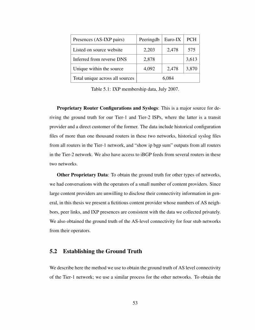
Presences (AS-IXP pairs) Peeringdb Euro-IX PCH

Listed on source website 2,203 2,478 575

Inferred from reverse DNS 2,878 3,613

Unique within the source 4,092 2,478 3,870

Total unique across all sources 6,084

Table 5.1: IXP membership data, July 2007.

Proprietary Router Configurations and Syslogs: This is a major source for de-

riving the ground truth for our Tier-1 and Tier-2 ISPs, where the latter is a transit

provider and a direct customer of the former. The data include historical configuration

files of more than one thousand routers in these two networks, historical syslog files

from all routers in the Tier-1 network, and “show ip bgp sum” outputs from all routers

in the Tier-2 network. We also have access to iBGP feeds from several routers in these

two networks.

Other Proprietary Data: To obtain the ground truth for other types of networks,

we had conversations with the operators of a small number of content providers. Since

large content providers are unwilling to disclose their connectivity information in gen-

eral, in this thesis we present a fictitious content provider whose numbers of AS neigh-

bors, peer links, and IXP presences are consistent with the data we collected privately.

We also obtained the ground truth of the AS-level connectivity for four stub networks

from their operators.

5.2 Establishing the Ground Truth

We describe here the method we use to obtain the ground truth of AS level connectivity

of the Tier-1 network; we use a similar process for the other networks. To obtain the

53

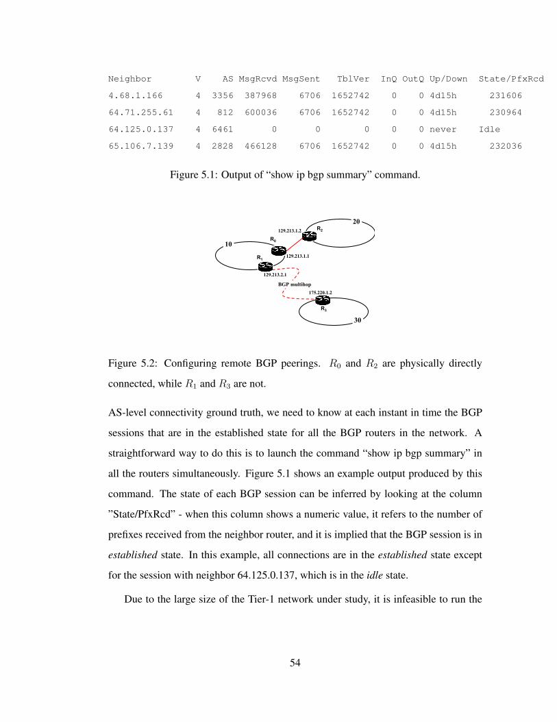
Neighbor V AS MsgRcvd MsgSent TblVer InQ OutQ Up/Down State/PfxRcd

4.68.1.166 4 3356 387968 6706 1652742 0 0 4d15h 231606

64.71.255.61 4 812 600036 6706 1652742 0 0 4d15h 230964

64.125.0.137 4 6461 0 0 0 0 0 never Idle

65.106.7.139 4 2828 466128 6706 1652742 0 0 4d15h 232036

Figure 5.1: Output of “show ip bgp summary” command.

10

20

129.213.1.1

129.213.1.2

BGP multihop

30

R0

R1

R2

R3

129.213.2.1

175.220.1.2

Figure 5.2: Configuring remote BGP peerings. R0 and R2 are physically directly

connected, while R1 and R3 are not.

AS-level connectivity ground truth, we need to know at each instant in time the BGP

sessions that are in the established state for all the BGP routers in the network. A

straightforward way to do this is to launch the command “show ip bgp summary” in

all the routers simultaneously. Figure 5.1 shows an example output produced by this

command. The state of each BGP session can be inferred by looking at the column

”State/PfxRcd” - when this column shows a numeric value, it refers to the number of

prefixes received from the neighbor router, and it is implied that the BGP session is in

established state. In this example, all connections are in the established state except

for the session with neighbor 64.125.0.137, which is in the idle state.

Due to the large size of the Tier-1 network under study, it is infeasible to run the

54

“show ip bgp sum” command over all the routers of the network and over a long study

period. It is also impossible to obtain any historic “show ip bgp sum” data for the

past. Therefore, we resort to an alternative way to infer the connectivity ground truth

- analyzing routers’ configuration files. Routers’ configuration files are a valuable

source of information about AS level connectivity. Before setting up a BGP session

with a remote AS, each router needs to have a minimum configuration state. As an

example, in Figure 5.2, for router R0 in AS10 to open a BGP session with R2 in AS20,

it needs to have a “neighbor 129.213.1.2 remote-as 20” entry in its configuration file,

as well as IP connectivity between R0 and R2 through a configured route to reach

R2. Similarly, R2 needs to have a configured route to reach R0. The IP connectivity

between the two routers of a BGP session can be established in one of the following

two ways:

• Single-hop: two routers are physically connected directly, as the case of R0

and R2 in Figure 5.2. More specifically R0 can (1) define a subnet for the lo-

cal interface at R0 that includes the remote address 129.213.1.2 of R2, e.g. “

ip address 129.213.1.1 255.255.255.252” (where 255.255.255.252 is the subnet

mask) or (2) set a static route in R0 to the remote address 129.213.1.2 of R2,

e.g. “ip route 129.213.1.0 255.255.255.252 Serial4/1/1/24:0” (in this case Se-

rial4/1/1/24:0 refers to the name of the local interface at R0).

• Multi-hop: two routers (such as R1 and R3 in Figure 5.2) are not directly con-

nected, but connected via other routers. To configure such a multi-hop BGP

session, R1 configures e.g. “neighbor 175.220.1.2 ebgp-multihop 3” (here 3

refers to the number of IP hops between R1 and R3); R1 reaches R3 by doing

longest prefix matching of 175.220.1.2 in its routing table.

Ideally, we would like to verify the existence of a BGP session by checking the

configuration files on both sides of a session. Unfortunately it is impossible to get

55

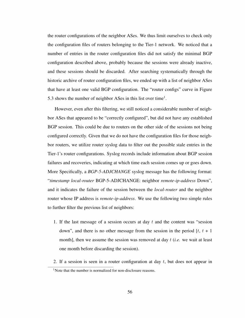
the router configurations of the neighbor ASes. We thus limit ourselves to check only

the configuration files of routers belonging to the Tier-1 network. We noticed that a

number of entries in the router configuration files did not satisfy the minimal BGP

configuration described above, probably because the sessions were already inactive,

and these sessions should be discarded. After searching systematically through the

historic archive of router configuration files, we ended up with a list of neighbor ASes

that have at least one valid BGP configuration. The “router configs” curve in Figure

5.3 shows the number of neighbor ASes in this list over time1.

However, even after this filtering, we still noticed a considerable number of neigh-

bor ASes that appeared to be “correctly configured”, but did not have any established

BGP session. This could be due to routers on the other side of the sessions not being

configured correctly. Given that we do not have the configuration files for those neigh-

bor routers, we utilize router syslog data to filter out the possible stale entries in the

Tier-1’s router configurations. Syslog records include information about BGP session

failures and recoveries, indicating at which time each session comes up or goes down.

More Specifically, a BGP-5-ADJCHANGE syslog message has the following format:

“timestamp local-router BGP-5-ADJCHANGE: neighbor remote-ip-address Down”,

and it indicates the failure of the session between the local-router and the neighbor

router whose IP address is remote-ip-address. We use the following two simple rules

to further filter the previous list of neighbors:

1. If the last message of a session occurs at day t and the content was “session

down”, and there is no other message from the session in the period [t, t + 1

month], then we assume the session was removed at day t (i.e. we wait at least

one month before discarding the session).

2. If a session is seen in a router configuration at day t, but does not appear in1Note that the number is normalized for non-disclosure reasons.

56

syslog for the period [t, t + 1 year], then we assume the session was removed at

day t (i.e. we wait at least 1 year before discarding the session).

Note that the above thresholds were empirically selected to minimize the number of

false positives and false negatives in the inferred ground truth. A smaller value would

increase the number of false negatives (i.e. sessions that are prematurely removed by

our scheme while still in the ground truth), whereas a higher value would increase the

false positives (i.e. sessions that are no longer in the ground truth, but have not been

removed yet by our scheme). We calibrated the thresholds using AS adjacencies that

were present in both the syslog messages and in the public view, e.g. we quantified the

false negatives by looking at adjacencies that we excluded using the syslog thresholds,

but were actually still visible in the public view. Even though these threshold values

worked well in this case, depending on the stability of links and routers’ configuration

state, other networks may require different values. Note also that these two rules are for

individual BGP sessions only. An AS-level link between the Tier-1 ISP and a neighbor

AS will be removed only when all of the sessions between them are removed by the

above two rules. The sessions between the Tier-1 ISP and its peers tend to be stable

with infrequent session failures [89], thus it is possible that a session never fails within

a year. But our second rule above is unlikely to remove the AS-level link between

the Tier-1 ISP and its peer because there are usually multiple BGP sessions between

them and the probability that none of the sessions have any failures for an entire year

is very small. Similarly, this argument is true for large customer networks which have

multiple BGP sessions with the Tier-1 ISP. On the other hand, small customers tend

to have a small number of sessions with the Tier-1 ISP (perhaps one or two), and the

sessions tend to be less stable thus have more failures and recoveries. Thus if the AS

link exists, the above two rules should not filter it out since some syslog session up

or down messages will be seen. For similar reasons, the results are not significantly

57

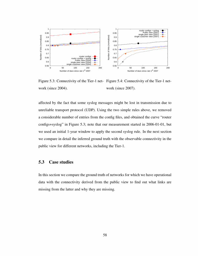
0.55

0.6

0.65

0.7

0.75

0.8

0.85

0.9

0.95

1

0 50 100 150 200

Num

ber

of li

nks

(nor

mal

ized

)


router configsrouter configs + syslog

Public view (2004)single peer view (2004)

single customer view (2004)

Figure 5.3: Connectivity of the Tier-1 net-

work (since 2004).

0.55

0.6

0.65

0.7

0.75

0.8

0.85

0.9

0.95

1

0 50 100 150 200

Num

ber

of li

nks

(nor

mal

ized

)


router configs + syslogPublic view (2007)

single peer view (2007)single customer view (2007)

Figure 5.4: Connectivity of the Tier-1 net-

work (since 2007).

affected by the fact that some syslog messages might be lost in transmission due to

unreliable transport protocol (UDP). Using the two simple rules above, we removed

a considerable number of entries from the config files, and obtained the curve “router

configs+syslog” in Figure 5.3; note that our measurement started in 2006-01-01, but

we used an initial 1-year window to apply the second syslog rule. In the next section

we compare in detail the inferred ground truth with the observable connectivity in the

public view for different networks, including the Tier-1.

5.3 Case studies

In this section we compare the ground truth of networks for which we have operational

data with the connectivity derived from the public view to find out what links are

missing from the latter and why they are missing.

58

0.55

0.6

0.65

0.7

0.75

0.8

0.85

0.9

0.95

1

0 50 100 150 200

Num

ber

of li

nks

(nor

mal

ized

)


router configs + syslogOregon RV RIB+updatesOregon RV RIB snapshot

Figure 5.5: Capturing the connectivity of

the Tier-1 network through table snap-

shots and updates.

0.6

0.65

0.7

0.75

0.8

0.85

0.9

0.95

1

0 20 40 60 80 100 120 140 160 180

Num

ber

of li

nks

(nor

mal

ized

)

Number of days since March 10th 2007

router configsPublic view

single customer viewsingle provider view

show ip bgp sumPublic view (show ip bgp sum)

Figure 5.6: Tier-2 network connectivity.

5.3.1 Tier-1 Network

Once we achieved a good approximation of the ground truth as described in the pre-

vious section, we compared it to the public view derived connectivity. For each day

t, we compared the list of ASes in the inferred ground truth Ttier1(t) obtained from

router configs+syslog, with the list of ASes seen in public view as connected to the

Tier-1 network up to day t. The “Public view (2004)” curve in Figure 5.3 is obtained

by accumulating public view BGP-derived connectivity since 2004. We first note that

all the Tier-1 ISP’s links to its peers and sibling ASes are captured by the public view.

In particular, we note that the public view captured all the peer-peer links of the Tier-1

ISP. The peer links of an AS are visible as long as a monitor resides in the AS itself,

or in any of the AS’s customers, or the customer’s customers. In fact the public view

captured all the peer-peer links for all tier-1 ASes, due to the small number of tier-1

networks and the fairly large set of monitors used by public view.

Comparing the “Public view (2004)” curve with the “router configs+syslog” curve

in Figure 5.3, we also note that there is an almost constant small gap, which is of the

59

0.65

0.7

0.75

0.8

0.85

0.9

0.95

1

0 50 100 150 200

Num

ber

of li

nks

(nor

mal

ized

)


Customer viewbecame available

router configsOregon RV RIB+updatesOregon RV RIB snapshot

Figure 5.7: Capturing Tier-2 network con-

nectivity through table snapshots and up-

dates.

60

70

80

90

100

110

120

130

0 100 200 300 400 500

Num

ber

of li

nks

Number of days since Feb 22nd 2006

show ip bgp sum, ipv4+ipv6show ip bgp sum, ipv4 only

Abilene eBGP feedPublic view

Figure 5.8: Abilene connectivity.

order of some tens of links (3% of the total links in “router configs+syslog”). We

manually investigated these links, and found that there are three main causes for why

they do not show up in the public view: (1) the links that connect to the Tier-1’s

customer ASes which only advertise prefixes longer than /24; these long prefixes are

then aggregated by the Tier-1 AS before announcing to other neighbors. This category

accounts for about half of the missing links; (2) there is one special purpose AS number

(owned by the Tier-1 ISP) which is only used by the Tier-1 ISP; (3) false positives,

i.e. ASes that were wrongly inferred as belonging to Ttier1(t), including stale entries,

as well as newly allocated ASes whose sessions were not up yet. The false positive

contributes to about half of the “missing links” (which should not be called ”missing”).

Figure 5.4 shows similar curves using the same vertical scale as in Figure 5.3,

but this time the public view BGP data collection is started in the beginning of 2007.

When comparing “Public view (2007)” and “router configs+syslog” we note the gap

is bigger, indicating that some entries in “router configs+syslog” did not show up in

public view after 2007, but they did show up before, which likely means they are stale

60

entries (false positives).

The “Single customer view” and “Single peer view” curves in both Figures 5.3 and

5.4 represent the Tier-1 connectivity as seen from a single router in a customer of the

Tier-1 ISP and a single router in a peer of the ISP, both from the public view. The sin-

gle peer view captures slightly less links than the single customer view, corresponding

to about ∼1.5% of the total number of links of the Tier-1 network. Further analysis

revealed that this small delta corresponds to the peer links of the Tier-1, which are

included in routes advertised to the customer but not advertised to the peer. This is

expected and consistent with the no-valley routing policy. We also note that the “Sin-

gle peer view” and “Single customer view” curves in Figure 5.4 show an exponential

increase in the first few days of the x-axis, which is caused by the revelation of hidden

links, as explained in Chapter 2. However, the nine months of the measurement should

be enough to reveal the majority of the hidden links [72]. In addition, note that in both

figures, the “Single customer view” curve is very close to the public view curve, which

means that the connectivity of the Tier-1 as seen by the customer is representative of

what is visible from the public view.

Figure 5.5 shows the difference between using routing table snapshots (RIB) ver-

sus using an initial RIB plus BGP updates from all the routers at Oregon RouteViews

(a subset of 46 routers of the entire public view). Note that on each day, the num-

ber of links in the curves “Oregon RV (RouteViews) RIB snapshot” and “Oregon RV

RIB+updates” represent the overlap with the set of links in the inferred ground truth

represented by the curve “router configs+syslog”, i.e. , those links not in “router con-

figs + syslog” are removed from the two “Oregon RV” curves. Even though both

curves start in the same point, after more than nine months of measurement, “Oregon

RV RIB+upates” reveals about 10% more links than those revealed by “Oregon RV

RIB snapshot”, these are the links that were revealed in BGP updates of alternative

61

routes encountered during path exploration as described in [71]. We also note that the

difference between the two curves are all customer-provider links, and all the Tier-1

ISP’s links to the peers are captured by the ”Oregon RV RIB snapshot”, because of the

large number of routes that go through these peer-peer links.

Summary:

• A single snapshot of the Oregon RV RIB can miss a noticeable percentage (e.g.,

10%) of the Tier-1’s AS-level links, all of them customer-provider links, when

compared to using RIBs plus updates accumulated in several months.

• The Tier-1 AS’s links are covered fairly completely by the public view over

time. All the peer-peer and sibling links are covered; the small percentage (e.g.,

1.5%) of links missing from public view are the links to customer ASes who

only announce prefixes longer than /24 and hence their routes are aggregated.

• The Tier-1 AS’s links are covered fairly completely by a single customer by us-

ing the historic BGP tables and updates, which can be considered representative

of the public view.

• The Tier-1 AS’s links are covered fairly completely by a single peer (when the

historic BGP table and updates are used), and the about 1.5% missing links are

all peer-peer links.

5.3.2 Tier-2 Network

The Tier-2 network we studied differs from the previous Tier-1 case in a few important

ways. First of all, not being a Tier-1 network, the Tier-2 has providers. Second, it

is considerably smaller in size as measured by the number of routers, however it has

considerably more peer links than the Tier-1 network. Third, the Tier-1 network peers

62

exclusively through private peering, this Tier-2 network had close to 23

of its peers

through IXPs. We do an analysis similar to the Tier-1 case, except that we did not have

access to syslog data.

The “router configs” curve in Figure 5.6 shows the number of neighbor ASes ob-

tained from router configurations over time. Let us assume for now this is a good

approximation of the ground truth of the Tier-2 network connectivity. We include in

Figure 2 two single router view curves, one is obtained from a router in a customer of

the Tier-2 network, and the other is derived from a router in a provider of the Tier-2

network, both are in the public view. Note that this time we started the measurement

in March 2007 when the BGP data for the customer router became available in the

public view. This customer router became unavailable after August 13, 2007, hence

the single customer view curve is chopped off after that date. Figure 5.6 shows that the

provider view misses a significant number of links that are captured by the customer

view. This difference amounts to more than 12% of the Tier-2’s links captured by the

customer, which are all the peer links of the Tier-2 network. For comparison, we also

included the public view curve, starting at March 10th 2007. Note that the public view

captured a very small number of neighbors that are not in the customer view. We found

that most of the links in this small gap were revealed in the routes that were originated

by the Tier-2’s customers and had several levels of AS prepending. The customer we

used for the customer view curve did not pick these routes because of the path inflation

due to the AS prepending, however following the prefer-customer policy, routers in the

Tier-2 network picked these prepended routes, and one of these routers is in the public

view data set.

From Figure 5.6 we also note that the connectivity captured by the public view is

∼85% of that inferred from router configs, which could be due to incorrect or stale

entries in the router configuration files. To verify whether this is the case, we launched

63

a “show ip bgp summary” command on all the routers of the network on 2007-09-03,

and we take into account only those BGP sessions that were in the established state.

The number of neighbors with at least one such session is shown in Figure 5.6 by the

“show ip bgp sum” point, which has only 80% of the connectivity inferred from the

router configurations. This means that about 20% of the connectivity extracted from

router configs were false positives. On the other hand, we observe that by accumulating

BGP updates over time, we also increase the number of false positives, i.e. adjacencies

that were active in the past and became inactive. By comparing the curves “Public

View” and “Public view (show ip bgp sum)”, we note that about 1 − 0.750.85' 0.12 (or

12%) of the links accumulated in public view over the 6-month period correspond to

false positives. There are however ways to filter these false positives: (1) by removing

the short-lived links, since most likely they correspond to misconfigurations, or (2) by

timing out links after a certain period of time. The point “Public view (show ip bgp

sum)” in the figure represents the intersection between the set of neighbors extracted

from “show ip bgp sum” and the set of neighbors seen so far in the public view. Note

that public view missed∼7% of the links given by “show ip bgp sum”, which amounts

to a few tens of links. One of these links was the RouteViews passive monitoring

feed, some other were internal AS numbers, and the remaining ones were to the ASes

announcing longer than /24 routes (that were aggregated). Note also that the fairly

complete coverage of the Tier-2 network’s connectivity is due to the existence of a

monitor residing in a customer of the Tier-2. As we explained in the Tier-1’s study,

the public view can capture all the links, including all peer links of an AS, if a monitor

resides in either the AS itself, or in the AS’s customer or customer’s customers.

Figure 5.7 shows the difference between using single RIB snapshot versus initial

RIB+updates from RouteViews Oregon collector, using the same vertical scale as in

Figure 5.6. In this case, using updates reveals ∼12% more links than those revealed

by router RIB snapshots in the long run. Note that there is a lack of configuration files

64

at beginning of 2007, hence the missing initial part on the curve “router configs”. The

jump in the figure is due to the addition of the monitor in the Tier-2 customer AS,

which revealed the peer links of the Tier-2 network.

Summary:

• A single snapshot of the Oregon RV RIB can miss a noticeable percentage (e.g.,

12%) of the Tier-2’s AS-level links, all of them customer-provider links, when

compared to using RIBs+updates accumulated in several months.

• The Tier-2 AS’s links are covered fairly completely by a single customer over

time (RIBs +updates), which can be considered representative of the entire pub-

lic view.

• A single provider view can miss a noticeable percentage (e.g., 12%) of the Tier-

2’s links, and all the missing links are peer-peer links.

• A Tier-2 AS’s links are covered fairly completely by the public view over time

if there is a monitor in it, or its customer or its customer’s customers, in which

case all the peer-peer links are revealed. The small percentage (e.g., 7%) of

links missing from the public view are those connecting to customers who only

announce prefixes longer than /24 or those ASes dedicated for internal use.

5.3.3 Abilene and Geant

Abilene: Abilene (AS11537) is the network interconnecting universities and research

institutions in the US. The Abilene Observatory [19] keeps archives of the output of

“show ip bgp summary” for all the routers in the network. Using this data set, we built

a list of Abilene AS neighbors over time, which is shown in the “show ip bgp sum,

ipv4+ipv6” curve in Figure 5.8. Even though Abilene does not provide commercial

65

transit, it enables special arrangements where its customers may inject their prefixes to

commercial providers through Abilene, and receive routes from commercial providers

through Abilene. The academic-to-commercial service is called Commercial Peer-

ing Service (or CPS) versus the default academic-to-academic Research & Education

(R&E) service. These two services are implemented by two different VPNs over the

Abilene backbone. BGP sessions for both VPNs are included in the output of “show ip

bgp summary”. We compare Abilene connectivity ground truth with that derived from

a single router eBGP feed (residing in Abilene) containing only the R&E sessions. In

addition, we do a similar comparison with our public view, which should contain both

CPS and R&E sessions (public view contains eBGP+iBGP Abilene feeds, as well as

BGP data from commercial providers of Abilene). However, since there are a consid-

erable number of neighbors in Abilene that are using IPv6 only, and since the BGP

data in our data set are mostly IPv4-only, we decided to place the IPv4-only neighbors

in a separate set. The curve “show ip bgp sum, ipv4 only” in Figure 5.8 shows only

the AS neighbors that have at least one IPv4 session connected to Abilene2. Contrary

to the “show ip bgp sum, ipv4+ipv6” curve which includes all sessions, the IPv4-only

curve shows a decreasing trend. We believe this is because some of the IPv4 neighbors

have been migrating to IPv6 over time. When comparing the “show ip bgp sum, ipv4

only” curve with the one derived from the eBGP feed, we find there is a constant gap

of about 10 neighbors. A closer look into these cases revealed that these AS num-

bers belonged to commercial ASes with sessions associated with the CPS service. The

small gap between the public view and the IPv4-only curve corresponds to the passive

monitoring session with RouteViews (AS6447).

Geant: Geant (AS20965) is an European research network connecting 26 R&E net-

works representing 30 countries across Europe. In contrast to Abilene where the focus

2Note that there was a period of time between days 350 and 475 for which there was no “show ipbgp sum” data from Abilene.

66

is on establishing academic-to-academic connectivity, Geant enables its members to

connect to the commercial Internet using its backbone. We inferred Geant connectiv-

ity ground truth by running the command “show ip bgp sum” in all its routers through

its looking glass site [5]. We found a total of 50 AS neighbors with at least one ses-

sion in the established state. By comparing Geant ground truth with the connectivity

revealed in public view, we found a match on all neighbor ASes except two. One of

the exceptions was a neighbor which was running only IPv6 multicast sessions, and

therefore hidden from public view which consists mostly of IPv4-only feeds. The other

exception seems due to a passive monitoring session to a remote site, which explains

why its AS number was missing from BGP feeds.

Summary: In Abilene and Geant, the public view matches the connectivity ground

truth (no invisible or hidden links), capturing all the customer-provider and peer links.

Abilene represents a special case, where depending on the viewpoint there can be in-

visible links. For instance, some Abilene connectivity may be invisible to its customers

due to the academic-to-commercial special arrangements.

5.3.4 Content provider

Content networks are fundamentally different from transit providers such as the Tier-1

and Tier-2 cases we studied earlier. Content networks are edge ASes and do not transit

traffic between networks, thus they only have peers and providers. They generally try

to reduce the amount of (more expensive) traffic sent to providers by directly peering

with as many other networks as possible; direct peerings can also help improve per-

formance. Consequently, content networks in general have a heavy presence at IXPs,

where they can peer with multiple different networks. While two transit providers

usually peer at every location where they have a common presence in order to disperse

traffic to closer exit-points, peering of content networks is more “data-driven” (versus

67

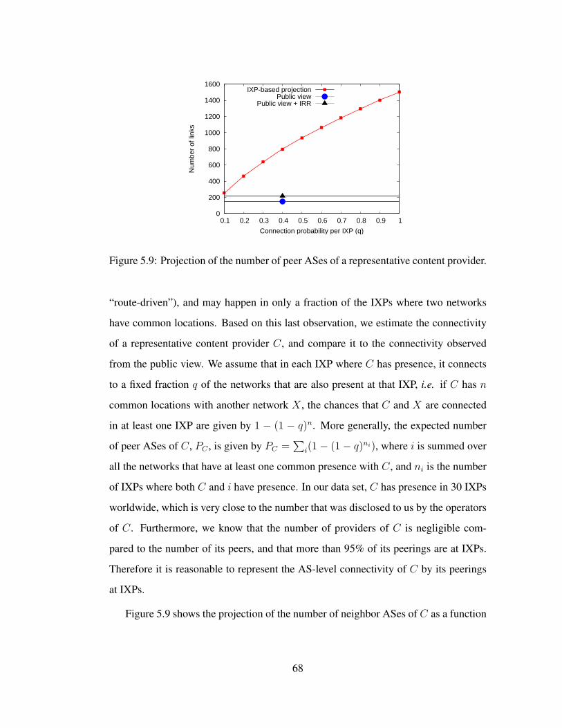
0

200

400

600

800

1000

1200

1400

1600

0.1 0.2 0.3 0.4 0.5 0.6 0.7 0.8 0.9 1

Num

ber

of li

nks

Connection probability per IXP (q)

IXP-based projectionPublic view

Public view + IRR

Figure 5.9: Projection of the number of peer ASes of a representative content provider.

“route-driven”), and may happen in only a fraction of the IXPs where two networks

have common locations. Based on this last observation, we estimate the connectivity

of a representative content provider C, and compare it to the connectivity observed

from the public view. We assume that in each IXP where C has presence, it connects

to a fixed fraction q of the networks that are also present at that IXP, i.e. if C has n

common locations with another network X , the chances that C and X are connected

in at least one IXP are given by 1 − (1 − q)n. More generally, the expected number

of peer ASes of C, PC , is given by PC =∑

i(1− (1− q)ni), where i is summed over

all the networks that have at least one common presence with C, and ni is the number

of IXPs where both C and i have presence. In our data set, C has presence in 30 IXPs

worldwide, which is very close to the number that was disclosed to us by the operators

of C. Furthermore, we know that the number of providers of C is negligible com-

pared to the number of its peers, and that more than 95% of its peerings are at IXPs.

Therefore it is reasonable to represent the AS-level connectivity of C by its peerings

at IXPs.

Figure 5.9 shows the projection of the number of neighbor ASes of C as a function

68

of the connection probability q at each IXP. For comparison purposes, we also include

the number of neighbor ASes of C as inferred from the public view over a window of

6 months. From discussions with C’s operators, we know that at each IXP, C peers

with about 80-95% of the participants at the IXP (parameter q), and that the total

number of BGP sessions of C is more than 2,000, even though we do not know the

total number of unique peer ASes3. In view of these numbers, the projection in Figure

5.9 seems reasonable, even after taking into account that our IXP membership data

is incomplete. The most striking observation is the amount of connectivity missed

from the public view, which is on the order of thousands of links and represents about

90% of C’s connectivity. This result is not entirely surprising, however, because based

on no-valley policy, the content provider C does not announce its peer-peer links to

anyone, and a peer-peer link is visible only if the public view has a monitor in C, or

in the peer or a customer of the peer. Yet the number of available monitors is much

smaller than the projected total number of C’s peer. We believe this result holds true

for other large content providers, search engines, and content distribution networks.

Trying to close the gap between reality and the public view, we looked for addi-

tional connectivity in the IRR, as described in Section 5.1. We discovered 62 additional

neighbor ASes for C that were not present in the initial set of 155 ASes seen in the

public view. Even though this addition increased the number of covered neighbor ASes

of C to 217, it is still only about 15% of the AS-level connectivity of C.

Summary: The public view misses about 90% of C’s connectivity, and we believe

all of them are invisible peer-peer links, and most of them are likely at IXPs. Using

IRR information reduces the missing connectivity slightly, to 85%. The public BGP

view’s inability to catch these peer-peer links is due to the no-valley policy and the

absence of monitors in the peers or their customers of the content network.

3The number of unique neighbor ASes is less than the total number of BGP sessions, as there existmultiple BGP sessions with the same neighbor AS.

69

5.3.5 Simple stubs

Stub networks are those ASes that do not have customers (or have a very small num-

ber of customers)4. Stubs represent the vast majority of ASes, and they are typically

sorted according to their business rationale into: 1)content, 2)eyeball and 3)simple.

Content networks have heavy outbound traffic, whereas eyeballs are heavy inbound

(e.g. cable/dsl providers). Simple stubs represent enterprise customers such as uni-

versities and small companies. We obtained the AS-level connectivity ground truth of

4 simple stubs by directly contacting their operators. Table 5.2 shows for each net-

work the number of neighbor ASes in the ground truth as reported by the operators, as

well as the number of neighbor ASes captured by the BGP-derived public view. Note

that for public view we use 6 month worth of BGP RIB and updates to accumulate

the topology to account for hidden links that take time to be revealed [72]. Network

D is the only case where there is a perfect match between ground truth and public

view. For network A, there are two neighbors included in public view that were dis-

connected during the 6-month window (false positives). For network B, the public

view was missing a neighbor due to a special agreement in which the routes learned

from the neighbor are not announced to B’s provider. Finally, for network C there was

an extra neighbor in public view that was never connected to C, but appeared in routes

during one day in the 6-month window. We believe this case was originated either by

a misconfiguration or a malicious false link attack.

Summary: The 6-month accumulated public view captured all the customer-provider

links of the stub networks studied. In total, the public view has one false negative (in-

visible link) and 3 false positives, the latter can be eliminated by reducing the interval

of the observation window of public view.

4The details about stub classification are describe in Section 5.4.2

70

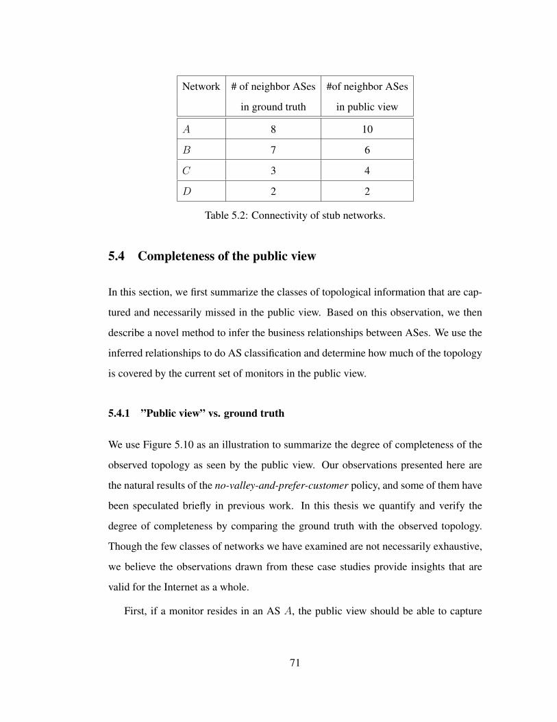
Network # of neighbor ASes #of neighbor ASes

in ground truth in public view

A 8 10

B 7 6

C 3 4

D 2 2

Table 5.2: Connectivity of stub networks.

5.4 Completeness of the public view

In this section, we first summarize the classes of topological information that are cap-

tured and necessarily missed in the public view. Based on this observation, we then

describe a novel method to infer the business relationships between ASes. We use the

inferred relationships to do AS classification and determine how much of the topology

is covered by the current set of monitors in the public view.

5.4.1 ”Public view” vs. ground truth

We use Figure 5.10 as an illustration to summarize the degree of completeness of the

observed topology as seen by the public view. Our observations presented here are

the natural results of the no-valley-and-prefer-customer policy, and some of them have

been speculated briefly in previous work. In this thesis we quantify and verify the

degree of completeness by comparing the ground truth with the observed topology.

Though the few classes of networks we have examined are not necessarily exhaustive,

we believe the observations drawn from these case studies provide insights that are

valid for the Internet as a whole.

First, if a monitor resides in an AS A, the public view should be able to capture

71

all of A’s direct links, including both customer-provider and peer links. However, not

all the links of the AS may show up in a snapshot observation. It takes time, which

may be as long as a few years, to have all hidden customer-provider links exposed by

routing dynamics. Second, a monitor in a provider network should be able to capture

all the provider-customer links between itself and all of its downstream customers, and

a monitor in a customer network should be able to capture all the customer-provider

links between itself and its upstream providers. For example, in Figure 5.10, a monitor

in AS2 can capture not only its direct provider-customer links (2-6 and 2-7), but also

the provider-customer links between its downstream customers (6-8, 6-9, 7-9, and 7-

10). AS5, as a peer of AS2, is also able to capture all the provider-customer links

downstream of AS2 since AS2 will announce its customer routes to its peers. Again,

it can take quite a long time to reveal all the hidden links. Third, a monitor cannot

observe a peer link of its customer, or peer links of its neighbors at the same tier 5. For

example, a monitor at AS5 will not be able to capture the peer link 6-7 or 1-2, because

a peer route is not announced to providers or other peers according to the no-valley

policy. Fourth, to capture a peer link requires a monitor in one of the peer ASes or in a

downstream customer of the two ASes incident to the link. For example, a monitor at

AS9 can observe the peer links 6-7 and 5-2, but not the peer link 1-3 since AS9 is not

a downstream customer of either AS1 or AS3.

The current public view has monitors in all the Tier-1 ASes except one, and that

particular Tier-1 AS has a direct customer AS that hosts a monitor. Applying the

above observations, we can summarize and generalize the completeness of the AS-

level topology captured by the public view as follows.

• Coverage of Tier-1 links: The public view contains all the links of all the Tier-1

ASes.5We assume that the provider-customer links do not form a circle.

72

• Coverage of customer-provider links: There is no invisible customer-provider

link. Thus over time the public view should be able to reveal all the customer-

provider links in the Internet topology, i.e. , the number of hidden customer-

provider links should gradually approach zero with the increase of the observa-

tion period length. This is supported by our empirical findings: in all our case

studies we found all the customer-provider links from BGP data collected over

a few years.

• Coverage of peer links: The public view misses a large number of peer links,

especially peer links between lower tier ASes in the Internet routing hierarchy.

The public view will not capture a peer link A–B unless there is a monitor

installed in either A or B, or in a downstream customer of A or B. Presently, the

public monitors are in about 400+ ASes out of a total over 27,000 existing ASes,

this ratio gives a rough perspective on the percentage of peer links missing from

the public view. Peer links between stub networks (i.e. , links 8-9 and 9-10 in

Figure 5.10) are among the most difficult ones to capture. Unfortunately, with

the recent growth of content networks, it is precisely these links that are rapidly

increasing in numbers.

5.4.2 Network Classification

The observations from the last section led us to a novel and simple method for inferring

the business relationships between ASes, that allow us also to classify ASes in different

types.

73

2


13

45

8

Tier-1

76

9 10

Propagation ofcustomer routes

Figure 5.10: Customer-provider links can

be revealed over time, but downstream

peer links are invisible to upstream mon-

itors.

0.8

0.82

0.84

0.86

0.88

0.9

0.92

0.94

0.96

0.98

1

0 20 40 60 80 100

Fre

quen

cy (

CD

F)

Number of customer ASes downstream

Figure 5.11: Distribution of number of

downstream customers per AS.

1

2 3


65

p

p

4

pinvisiblelink

Figure 5.12: Example of a prefix hijack scenario where AS2 announces prefix p be-

longing to AS1. Because of the invisible peer link AS2–AS3, the number of ASes

affected by the attack is underestimated.

74

5.4.2.1 Inferring AS Relationships

The last section concluded that, assuming routes follow a no-valley policy, monitors

at the top of the routing hierarchy (i.e. those in Tier-1 ASes) are able to reveal all the

downstream provider-customer connectivity over time. This is an important observa-

tion since, by definition, each non-Tier-1 AS is a customer of at least one Tier-1 AS,

then essentially all the provider-customer links in the topology can be observed by

the Tier-1 monitors over time. This is the basic idea of our AS relationship inference

algorithm.

We start with the assumption that the set of Tier-1 ASes is already known6. By

definition of Tier-1 ASes, all links between Tier-1s are peer links, and a Tier-1 AS

is not a customer of any other ASes. Suppose a monitor at Tier-1 AS m reveals an

ASPATH m-a1-a2-...-an. The link m-a1 can be either a provider-customer link, or a

peer link (this is because in certain cases a Tier-1 may have a specially arranged peer

relationship with a lower-tiered AS). However, according to the no-valley policy, a1-

a2, a2-a3, ... , an−1-an must be provider-customer links, because a peer or provider

route should not be propagated upstream from a1 to m. Therefore the segment a2, ...,

an must correspond to a customer route received by a1. To infer the relationship of

m-a1, we note that according to no-valley policy, if m-a1 is a provider-customer link,

this link should appear in the routes propagated from m to other Tier-1 ASes, whose

monitors will reveal this link. On the other hand, if m-a1 is a peer link, it should

never appear in the routes received by the monitors in other Tier-1 ASes. Given we

have monitors in all Tier-1 ASes or their customer ASes, we can accurately infer the

relationship m-a1 by examining whether it is revealed by other Tier-1 ASes. Using

this method, we can first find and label all the provider-customer links, and then label

all the other links revealed by the monitors as peer links.6The list of Tier-1 ASes can be obtained from website such as

http://en.wikipedia.org/wiki/Tier 1 carrier

75

Our algorithm is illustrated in Figure 5.10, where 1, 2, 3, and 4 are known to be

Tier-1s. Suppose AS 2 monitor reveals an ASPATH 2-5-6-8 and another ASPATH 2-

7-9; while monitors at AS 4 reveals an ASAPTH 4-2-7-9, but none of 1, 3, 4 reveals

an ASPATH with segment of 2-5-6-8. According to our new method, 5-6, 6-8, and

7-9 are definitely provider-customer links. 2-7 is a provider-customer link since it is

revealed by Tier-1s other than 2, while 2-5 is a peer link since it is not revealed by any

other Tier-1s. Furthermore, suppose AS 6 is a monitor and it reveals link 6-7, and 6-7

is never revealed by Tier-1 ASes 1,2,3, or 4. Then we can conclude that this 6-7 is a

peer link.

From BGP data collected from all the Tier-1 monitors over a 7-month period, we

were able to infer a total of 70,698 provider-customer links. We also noticed that a

small number of these links only existed in routes that had a very short lifetime (less

than 2 days). These cases are most likely caused by BGP misconfigurations (e.g. route

leakages) or route hijacks, as described in [61]. After filtering all the routes with a

lifetime less than 2 days over the 7-month measurement period, we excluded 5,239

links, ending up with a total of 65,459 provider-customer links. Note that even though

our relationship inference has the advantage of being simple, its accuracy can still be

improved. For instance, we could use the algorithm in [42] to select a maximal set of

AS paths that do not create cycles in relationships and are valley-free, and only con-

sider such relationships as valid. Note that out algorithm differs from the classic Gao’s

algorithm [39] in several ways. First, our algorithm is able to infer all the customer

provider relations based only in a very limited number of sources (the Tier-1 routers).

Second, contrary to [39], we do not rely on node degree to infer peer relationships. In

fact, the node degree is a variable of the monitor set, and that is the main reason why

[39] produces so distinct results with varying monitor sets. Our inference of peer rela-

tionships is purely based on the no-valley premise that peer routes are not propagated

upstream, therefore we believe our inference results are more accurate.

76

5.4.2.2 AS classification

AS classification schemes are typically based on each AS’s node degree (the num-

ber of neighbors) or the number of prefixes originated. However, the degree can be

misleading since it is a mix of providers, peers and customers in one count, and the

number of prefixes originated is not very reliable either since the length of the prefixes

is different and the routes carried downstream are not accounted. With the inferred

provider-customer relations in hand, we decided to use the number of downstream

customer ASes (or “customer cone”) as also defined in [34]. Figure 5.11 shows the

distribution of the number of downstream customers per AS. We note that over 80%

of the ASes have no customers, and a noticeable fraction of ASes have a very small

number of customers. We label as stub those ASes with 4 or less customers, which

encompass about 92% of the ASes. This should correspond to end networks which

either don’t provide transit or have very limited transit to few local customers, e.g.

universities providing transit to small local research facilities. Based on the knee of

the distribution in Figure 5.11, we label as small ISPs those ASes with between 5 and

50 downstream customers. They correspond to about 6% of the total ASes. The re-

maining non-tier-1 ASes in the long tail are labeled as large ISPs. Table 5.4 shows the

number of ASes in each class. We analyzed the sensitivity of the classification thresh-

olds by changing their values by some delta, and did not notice significant difference

in the end result.

5.4.3 Coverage of the public view

With our new method for AS relationship inference and AS classification, we now

attempt a rough quantification of the completeness of the AS topology as observed by

the public view. According to our observations in 5.4.1, a monitor can uncover all

the upstream connectivity over time. For example, in Figure 5.10, a monitor at AS

77

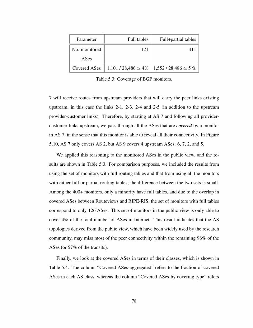
Parameter Full tables Full+partial tables

No. monitored 121 411

ASes

Covered ASes 1,101 / 28,486 ' 4% 1,552 / 28,486 ' 5 %

Table 5.3: Coverage of BGP monitors.

7 will receive routes from upstream providers that will carry the peer links existing

upstream, in this case the links 2-1, 2-3, 2-4 and 2-5 (in addition to the upstream

provider-customer links). Therefore, by starting at AS 7 and following all provider-

customer links upstream, we pass through all the ASes that are covered by a monitor

in AS 7, in the sense that this monitor is able to reveal all their connectivity. In Figure

5.10, AS 7 only covers AS 2, but AS 9 covers 4 upstream ASes: 6, 7, 2, and 5.

We applied this reasoning to the monitored ASes in the public view, and the re-

sults are shown in Table 5.3. For comparison purposes, we included the results from

using the set of monitors with full routing tables and that from using all the monitors

with either full or partial routing tables; the difference between the two sets is small.

Among the 400+ monitors, only a minority have full tables, and due to the overlap in

covered ASes between Routeviews and RIPE-RIS, the set of monitors with full tables

correspond to only 126 ASes. This set of monitors in the public view is only able to

cover 4% of the total number of ASes in Internet. This result indicates that the AS

topologies derived from the public view, which have been widely used by the research

community, may miss most of the peer connectivity within the remaining 96% of the

ASes (or 57% of the transits).

Finally, we look at the covered ASes in terms of their classes, which is shown in

Table 5.4. The column “Covered ASes-aggregated” refers to the fraction of covered

ASes in each AS class, whereas the column “Covered ASes-by covering type” refers

78

Type ASes Monitored Covered ASes

ASes aggregated by covering type

Tier-1 9 8 9 (100%) 8

Large ISP 436 45 337 (77.3%) 954

Small ISP 1,829 36 629 (34.4%) 269

Stubs 26,209 37 126 (0.5%) 160

Table 5.4: Coverage of BGP monitors for different network types.

to the total number of ASes covered by the monitors in each class. For instance, 77.3%

of the large ISPs are covered by monitors, and monitors in large ISPs cover a total of

954 total ASes. The numbers in the table indicate that Tier-1s are fully covered, large

ISPs are mostly covered, small ISPs remain largely uncovered (just 34.4%), and stubs

are almost completely uncovered (99.5%). These results are due to the fact that most

of the monitors reside in the core of the network. In order to cover a stub, we would

need to place a monitor in that stub, which is infeasible due to the very large number

of stubs in Internet.

5.5 Discussion

The defects in the inferred AS topologies, as revealed by our case studies, may have

different impacts on the different research projects and studies that use an inferred AS

topology. In the following, we use a few specific examples to illustrate some of the

problems that can arise.

Stub AS growth rates and network diameter: Given that the public view captures

almost all the AS nodes and customer-provider links, it provides an adequate data

source for studies on AS-topology metrics including network diameter; growth rates

79

and trends for the number of stub ASes; and quantifying customer multihoming (where

multihoming here does not account peer links).

Other graph-theoretic metrics: Given that the public view is largely inadequate in

covering peer links, and given that these peer links typically allow for shortcuts in

the data plane, relying on the public view can clearly cause major distortions when

studying generic graph properties such as node degrees, path lengths, node clustering,

etc.

Impact of prefix hijacking: Prefix hijacking is a serious security threat facing In-

ternet and happens when an AS announces prefixes that belong to other ASes. Recent

work on this topic [53, 100, 22, 92] evaluates the proposed solutions by using the in-

ferred AS topologies from the public view. Depending on the exact hijack scenario, an

incomplete topology can lead to either an underestimate or overestimate of the hijack

impact. Figure 5.12 shows an example of a hijack simulation scenario, where AS2

announces prefix p that belongs to AS1. Because of the invisible peer link 1–2, the

number of impacted ASes is underestimated, i.e. ASes 3,5 and 6 are believed to pick

the route originated by AS1, whereas in reality they would pick the more preferred

peer route coming from the hijacker AS2. At the same time, an incomplete topology

could also lead simulations to overestimate the impact of a hijack. For example, the

content network C considered in Section 5.3 has a large number of direct peers who

are unlikely to be impacted by a hijack from a remote AS, so missing 90% of C’s peer

links in the topology would significantly overestimate the impact of such a hijack. On

the other hand, if C is a hijacker, then the incomplete topology would result in a vast

underestimation of the impact.

Relationship inference/path inference: Several studies have addressed the problem

of inferring the relationship between ASes based on observed routing paths [39, 85,

63]. There can be cases where customer-provider links are wrongly inferred as peer

80

links based on the observed set of paths, creating a no-valley violation. Knowledge

of the invisible peer links in paths could avoid some of these errors. The path infer-

ence heuristics [63, 67, 68] are also impacted by the incompleteness problem, mainly

because they a priori exclude all paths that traverse invisible peer links.

Routing resiliency to failures: Studies that address robustness properties of the

Internet under different failure scenarios (e.g., see [35, 92]) also heavily depend on

having a complete and accurate AS-level topology, on top of which failures are sim-

ulated. One can easily envision scenarios where two parts of the network are thought

to become disconnected after a failure, while in reality there are invisible peer links

connecting them. Given that currently inferred AS maps tend to miss a substantial

number of peer links, robustness-related claims based these inferred maps need to be

viewed with a grain of salt.

Evaluation of new inter-domain protocols: The evaluation of new inter-domain

routing protocols also heavily relies on the accuracy of the AS-level topology over

which a new protocol is supposed to run. For instance, [87] proposes a new protocol

where a path-vector protocol is used among Tier-1 ASes, and all the ASes under each

Tier-1 run link-state routing. The design is based on an assumption that customer trees

of Tier-1 ASes are largely disjoint, and violations of this assumption are handled as

rare exceptions. However, in view of our findings, there are a substantial number of

invisible peer links interconnecting ASes at lower tier and around the edge of Internet,

therefore connectivity between different customer trees becomes the rule rather than

the exception. We would imagine the performance of the proposed protocol under

complete and incomplete topologies to be different, possibly quite significantly.

81

CHAPTER 6

Path Exploration and Internet Topology

In this chapter we study how the topology structure and relationship between different

networks constrain the path exploration process that occurs in BGP.

6.1 BGP Path Exploration

A number of previous analytical and measurement studies ([51, 52, 62]) have shown

the existence of BGP path exploration and slow convergence in the operational Internet

routing system, which can potentially lead to severe performance problems in data

delivery. Path exploration suggests that, in response to path failures or routing policy

changes, some BGP routers may try a number of transient paths before selecting a

new best path or declaring unreachability to a destination. Consequently, a long time

period may elapse before the whole network eventually converges to the final decision,

resulting in slow routing convergence. An example of path exploration is depicted in

Figure 6.1, where node C’s original path to node E (path 1) fails due to the failure of

link D-E. C reacts to the failure by attempting two alternative paths (paths 2 and 3)

before it finally gives up. The experiments in [51, 52, 62] show that some BGP routers

can spend up to several minutes exploring a large number of alternate paths before

declaring a destination unreachable.

The analytical models used in the previous studies tend to represent worst case sce-

narios of path exploration [51, 52], and the measurement studies have all been based

82

D

A B

C

E

3

1

2

X

Figure 6.1: Path exploration triggered by a fail-down event.

on controlled experiments with a small number of beacon prefixes. In the Internet op-

erational community there exist various different views regarding whether BGP path

exploration and slow convergence represent a significant threat to the network perfor-

mance, or whether the severity of the problem, as shown in simulations and controlled

experiments, would be rather rare in practice. A systematic study is needed to quantify

the pervasiveness and significance of BGP slow convergence in the operational routing

system.

6.2 Methodology and Data Set

Previous measurement results on BGP slow convergence were obtained through con-

trolled experiments. In these experiments, a small number of “beacon” prefixes are

periodically announced and withdrawn by their origin ASes at fixed time intervals [11,

13], and the resulting routing updates are collected at remote monitoring routers and

analyzed. In addition to generate announcements and withdrawals (Tup and Tdown

events), one can also use a beacon prefix to generate Tlong events by doing AS prepend-

ing [51]. For a given beacon prefix, because one knows exactly what, when, and where

83

is the root cause of each routing update, one can easily measure the routing conver-

gence time by calculating the difference between when the root cause is triggered and

when the last update due to the same root cause is observed. Although routing up-

dates for beacon prefixes may also be generated by unexpected path changes in the

network, those updates can be clearly identified through the use of anchor prefixes as

explained later in this section. Unfortunately one cannot assess the overall Internet

routing performance from observing the small number of existing beacon prefixes.

Our observation of routing dynamics is based on a set of routers termed monitors,

that propagate their routing table updates to collector boxes, which store them in disk

(e.g. RouteViews[15]). To obtain a comprehensive understanding of BGP path ex-

plorations in the operational Internet, we first cluster routing updates from the same

monitor and for the same prefix into events, sort all the routing events into several

classes, and then measure the duration and number of paths explored for each class of

events. Our task is significantly more difficult than measuring the convergence delay

of beacon prefixes for the following reasons. First, there is no easy way to tell whether

a sequence of routing updates is due to the same, or different root causes in order

to properly group them into events. Second, upon receiving an update for a prefix,

one cannot tell what is the root cause of the update, as is the case with beacon pre-

fixes. Furthermore, when the path to a given destination prefix changes, it is difficult

to determine whether the new path is a more, or less, preferred path compared to the

previous one, i.e. whether the prefix experiences a Tshort or a Tlong event in our event

classification.

To address the above problems, we take advantage of beacon updates to develop

and calibrate effective heuristics and then apply them to all the prefixes. In the rest of

this section, we first describe our data set, then discuss how we use beacon updates to

validate a timer-based mechanism for grouping routing updates into events, and how

84

we use beacon updates to develop a usage-based path ranking method which is then

used in our routing event classifications.

6.2.1 Data Set and Preprocessing

To develop and calibrate our update grouping and path ranking heuristics, we used

eight BGP beacons, one from PSG [11] (psg01), the other seven from RIPE [13]

(rrc01, rrc03, rrc05, rrc07,rrc10, rrc11 and rrc12). All the eight beacon prefixes are

announced and withdrawn alternately every 2 hours. We preprocessed the beacon up-

dates following the methods developed in [62]. First, we removed from the update

stream all the duplicate updates, as well as the updates that differ only in COMMU-

NITY or MED attribute values, because these updates are usually caused by internal

dynamics inside the last-hop AS. Second, we used the anchor prefix of each beacon to

detect routing changes other than those generated by the beacon origins. An anchor

prefix is a separate prefix announced by a beacon prefix’s origin AS, and is never with-

drawn after its announcement. Thus it serves as a calibration point to identify routing

events that are not originated by the beacon injection/removal mechanism. Because the

anchor prefix shares the same origin AS, and hopefully the same routing path, with the

beacon prefix, any routing changes that are not associated with the beacon mechanism

will trigger routing updates for both the anchor and the beacon prefixes. To remove

all beacon updates triggered by such unexpected routing events, for each anchor prefix

update at time t, we ignore all beacon updates during the time window [t−W, t+W ].

We set W ’s value to 5 minutes, as the results reported in [62] show that the number of

beacon updates remains more or less constant forW > 5 minutes. After the above two

steps of preprocessing, beacon updates are mainly comprised of those triggered by the

scheduled beacon activity at the origin ASes.

To assess the degree of path exploration for all the prefixes in the global routing

85

table, we used the public BGP data collected from 50 full-table monitoring points by

RIPE [14] and RouteViews [15] collectors during the months of January and Febru-

ary 2006. We used the data from January to evaluate the different path comparison

metrics and we later analyzed the events in both months. We removed from the data

all the updates that were caused by BGP session resets between the collectors and the

monitors, using the minimum collection time method described in [97]. Those updates

correspond to BGP routing table transfers between the collectors and the monitors, and

therefore should not be accounted in our study of the convergence process.

The 50 monitors were chosen based on the fact that each of them provided full

routing tables and continuous routing data during our measurement period. One month

was chosen as our measurement period based on the assumption that ISPs are unlikely

to make many changes of their interconnectivity within one month period, so that we

can assume the AS level topology did not change much over our measurement time

period, an assumption that is used in our AS path comparison later in the thesis.

6.2.2 Clustering Updates into Events

Some of the previous BGP data analysis studies [79, 25, 38] developed a timer-based

approach to cluster routing updates into events. Based on the observation that BGP

updates come in bursts, two adjacent updates for the same prefix are assumed to be due

to the same routing event if they are separated by a time interval less than a threshold

T . A critical step in taking this approach is to find an appropriate value for T . A value

that is too high can incorrectly group multiple events into one. On the other hand, a

value that is too low may divide a single event into multiple ones. Since the root causes

of beacon routing events are known, and the beacon update streams contain little noise

after the preprocessing, we use beacon prefixes to find an appropriate value for T .

Figure 6.2 shows the distribution of update inter-arrival times of the eight beacon

86

prefixes as observed from the 50 monitors. All the curves start flattening out either

before or around 4 minutes (the vertical line in the figure). If we use 4 minutes as

the threshold value to separate updates into different events, i.e. T = 4 minutes, in

the worst case (rrc01 beacon) we incorrectly group about 8% of messages of the same

event into different events; this corresponds to the inter-arrival time difference between

the cutting point of the rrc01 curve at 4 minutes and the horizontal tail of the curve. The

tail drop of all the curves at 7200 seconds corresponds to the 2-hour interval between

the scheduled beacon prefix activities 1.

Although the data for the beacon updates suggests that a threshold of T = 4 min-

utes may work well for grouping updates into events, no single value of T would be a

perfect fit for all the prefixes and all the monitors. Thus we need to assess how sensitive

our results may be with the choice of T = 4 minutes. Figure 6.3 compares the result

of using T = 4 minutes with that of T = 2 minutes and T = 8 minutes for clustering

the updates of all the prefixes collected from all the 50 monitors during our one-month

measurement period. Let E(m, p, 4) be the number of events identified by monitor m

for prefix p using T = 4 minutes; E(m, p, 2) and E(m, p, 8) are similarly defined but

with T = 2 minutes and T = 8 minutes respectively. Figure 6.3 shows the distribution

of |E(m, p, 8)−E(m, p, 4)| and |E(m, p, 2)−E(m, p, 4)|, which reflects the impact of

using a higher or lower timeout value, respectively. As one can see from the figure, in

about 50% of the cases the three different T values result in the same number of events,

and in more than 80% of the cases the results from using the different T values differ

by at most 2 events. Based on the data we can conclude that the result of event cluster-

ing is insensitive to the choice of T = 4 minutes. This observation is also consistent

1The psg01 curve reaches a plateau earlier than the other curves, indicating that it suffers less fromslow routing convergence. However one may note its absence of update inter-arrivals between 100seconds and 3600 seconds, followed by a high number of inter-arrivals around 3600 seconds. As hintedin [62], this behavior could be explained by BGP’s route flat damping, and one hour is the defaultmaximum suppression time applied to an unstable prefix when its announcement goes through a routerwhich enforces BGP damping.

87

0

0.1

0.2

0.3

0.4

0.5

0.6

0.7

0.8

0.9

1

1 10 100 1000 10000

CC

DF

Inter-arrival time (s)

psg01rrc01rrc03rrc12

rrc{05,07,10,11}

Figure 6.2: CCDF of inter-arrival times of

BGP updates for the 8 beacon prefixes as

observed from the 50 monitors.

0.5

0.6

0.7

0.8

0.9

1

0 1 2 3 4 5 6

Fre

quen

cy (

CD

F)

Difference in number of events per [monitor,prefix]

2 min8 min

Figure 6.3: Difference in number of events

per [monitor,prefix] for T=2 and 8 min-

utes, relatively to T=4 minutes, during one

month period.

88

Tdown TshortTup Tlong

Same Path

Observed Events

Path Disturbance Path Change

Tpdist Tequal Tspath

Figure 6.4: Event taxonomy.

with previous work. For example [38] experimented with various timeout threshold

values between 2 minutes and 16 minutes, and found no significant difference in the

clustering results. In the rest of the thesis, we use T = 4 minutes.

6.2.3 Classifying Routing Events

After the routing updates are grouped into events, we classify the events into different

types based on the effect that each event has on the routing path. Let us consider two

consecutive events n and n+ 1 for the same prefix observed by the same monitor. We

define the path in the last update of event n as the ending path of event n, which is

also the starting path for event n+ 1. Let pstart and pend denote an event’s starting and

ending paths, respectively, and ε denote the path in a withdrawal message (representing

an empty path). If the last update in an event is a withdrawal, we have pend = ε. Based

on the relation between pstart and pend of each event, we classify all the routing events

into one of the following categories as shown in Figure 6.4 2.

1. Same Path (Tspath): A routing event is classified as a Tspath if its pstart = pend,

and every update in the event reports the same AS path as pstart, although they

may differ in some other BGP attribute such as MED or COMMUNITY value.

Tspath events typically reflect the routing dynamics inside the monitor’s AS.

2To establish a valid starting state, we initialize pstart for each (monitor,prefix) pair with the pathextracted from the routing table of the corresponding monitor.

89

2. Path Disturbance (Tpdist): A routing event is classified as Tpdist if its pstart =

pend, and at least one update in the event carries a different AS path. In other

words, the AS path is the same before and after the event, with some transient

change(s) during the event. Tpdist events are likely resulted from multiple root

causes, such as a transient failure closely followed by a quick recovery, hence

the name of the event type. When multiple root causes occur closely in time,

the updates they produce also follow each other very closely, and no timeout

value would be able to accurately separate them out by the root causes. In our

study we identify these Tpdist events but do not include them in the convergence

analysis.

3. Path Change: A routing event is classified as a path change if its pstart 6= pend.

In other words, the paths before and after the event are different. Path change

events are further classified into five categories, based on whether the destina-

tion becomes available or unavailable, or changed to a more preferred or less

preferred path, at the end of the event. Let pref(p) represent a router’s prefer-

ence of path p, with a higher value representing a higher preference.

• Tup: A routing event is classified as a Tup if its pstart = ε. A previously

unreachable destination becomes reachable through path pend by the end of

the event.

• Tdown: A routing event is classified as Tdown if its pend = ε. That is, a

previously reachable destination becomes unreachable by the end of the

event.

• Tshort: A routing event is classified as Tshort if its pstart 6= ε, pend 6= ε and

pref(pend) > pref(pstart), indicating a reachable destination has changed

the path to a more preferred one by the end of the event.

90

• Tlong: A routing event is classified as a Tlong event if its pstart 6= ε, pend 6=

ε and pref(pend) < pref(pstart), indicating a reachable destination has

changed the path to a less preferred one by the end of the event.

• Tequal: A routing event is classified as Tequal if its pstart 6= ε, pend 6= ε and

pref(pend) = pref(pstart). That is, a reachable destination has changed

the path by the end of the event, but the starting and ending paths have the

same preference.

A major challenge in event classification is how to differentiate between Tlong and

Tshort events, a task that requires judging the relative preference between two given

paths. Individual routers use locally configured routing policies to choose the most

preferred path among available ones. Because we do not have precise knowledge of the

routing policies, we must derive effective heuristics to infer a routers’ path preference.

It is possible that our heuristics label two paths with equal preference, in which case

the event will be classified as Tequal. However, a good path ranking heuristic should

minimize such ambiguity.

6.2.4 Comparing AS Paths

If a routing event has non-empty pstart and pend, then the relative preference between

pstart and pend determines whether the event is a Tlong or Tshort. In the controlled

experiments using beacon prefixes, one can create such events by manipulating AS

paths. For example in [51], AS paths with length up to 30 AS hops were used to

simulate Tlong events.

However in general there has been no good way to infer routers’ preferences among

multiple available AS paths to the same destination. Given a set of available paths,

a BGP router chooses the most preferred one through a decision process. During

91

this process, the router usually considers several factors in the following order: local

preference (which reflects the local routing policy configuration), AS path length, the

MED attribute value, IGP cost, and tie-breaking rules. Some of the previous efforts in

estimating path preference tried to emulate a BGP router’s decision process to various

degrees. For example, [51, 52, 38] used path length only. Because BGP is not a

shortest-path routing protocol, however, it is known that the most preferred BGP paths

are not always the shortest paths. In addition, there often exist multiple shortest paths

with equal AS hop lengths. There are also a number of other efforts in inferring AS

relationship and routing policies. However as we will show later in this section, none

of the existing approaches significantly improves the inference accuracy.

To infer path preference with a high accuracy for our event classification, we took

a different approach from all the previous studies. Instead of emulating the router’s de-

cision process, we propose to look at the end result of the router’s decision: the usage

time of each path. The usage time is defined as the cumulative duration of time that

a path remains in the router’s routing table for each destination (or prefix). Assuming

that the Internet routing is relatively stable most of the time and failures are recovered

promptly, then most preferred paths should be used most and thus remain in the routing

table for the longest time. Given our study period is only one month, during this time

period it is unlikely that significant changes happened to routing policies and/or ISP

peering connections in the Internet. Thus we conjecture that relative preferences of

routing paths remained stable for most, if not all, the destinations during our study pe-

riod. Figure 6.5 shows the path usage time distribution for the monitor with IP address

12.0.1.63 (AT&T). The total number of distinct ASPATH-prefix pairs that appeared in

this router’s routing table during the month is slightly less then 650,000 (correspond-

ing to about 190,000 prefixes). About 23% of the ASPATH-prefix pairs (the 150,000

on the left side of the curve) stayed in the table for the entire measurement period, and

about 500,000 ASPATH-prefix pairs appeared in the routing table for only a fraction

92

1

10

100

1000

10000

100000

1e+06

1e+07

0 100000 200000 300000 400000 500000 600000

Pat

h U

sage

Tim

e (s

)

ASPATH-Prefix pair

Figure 6.5: Usage time per ASPATH-Prefix for router 12.0.1.63, Jan 2006.

of the period, ranging from a few days to some small number of seconds.

We compare this new Usage Time based approach with three other existing meth-

ods for inferring path preference: Length, Policy, and Policy+Length. Usage Time

uses the usage time to rank paths. Length infers path preference according the AS path

length. Policy is derives path preference based on inferred inter-AS relationships. We

used the algorithm developed in [39] to classify the relationships between ASes into

customer, provider, peer, and sibling. A path that goes through a customer is preferred

over a path that goes through a peer, which is preferred over a path that goes through

a provider 3. Policy+Length infers path preference by using the policies first, and then

using AS length for those paths that have the same AS relationship.

One challenge in conducting this comparison is how to verify the path ranking re-

sults without knowing the router’s routing policy configurations. We tackle this prob-

lem by leveraging our understanding about Tdown and Tup events. During Tdown events,

routers explore multiple paths in the order of decreasing preference; during Tup events,

routers explore paths in the order of increasing preference. Since we can identify Tdown

and Tup events fairly accurately, we can use the information learned from these events

to verify the results from different path ranking methods.

3We ignore those cases in which we could not establish the policy relation between two ASes. Suchcases happened in less than 1% of the total paths.

93

In an ideal scenario where paths explored during a Tdown (or Tup) event follow a

monotonically decreasing (or increasing) preference order, we can take samples of ev-

ery consecutive pair of routing updates and rank order the paths they carried. However

due to the difference in update timing and propagation delays along different paths,

the monotonicity does not hold true all the time. For example, we observed path with-

drawals appearing in the middle of update sequences during Tdown events. Therefore,

instead of comparing the AS paths carried in adjacent updates during a routing event,

we compare the paths occurred during an event with the stable path used either be-

fore or after the event. Figure 6.6 shows our procedure in detail. All the updates in

the figure are for the same prefix P . Before the Tup event occurs, the router does

not have any route to reach P . The first four updates are clustered into a Tup event

that stabilizes with path p4. After p4 is in use for some period of time, the prefix P

becomes unreachable. During the Tdown event, paths p5 and p6 are tried before the

final withdrawal update. From this example, we can extract the following pairs of

path preference: pref(p1) < pref(p4), pref(p2) < pref(p4), pref(p3) < pref(p4),

pref(p5) < pref(p4), and pref(p6) < pref(p4).

After extracting path preference pairs from Tdown and Tup events, we apply the

four path ranking methods in comparison to the same set of routing updates and see

whether they produce the same path ranking results as we derived from Tdown and

Tup events. We keep three counters Ccorrect, Cequal and Cwrong for each method. For

instance, in the example of Figure 6.6, if a method results in p1 and p2 being worse than

p4, and p3 having the same preference of p4 (equal), then for the Tup event we have

Ccorrect = 2 , Cequal = 1 and Cwrong = 0. Likewise, for the Tdown event, if a method

results in p5 being better than p4 and p6 being equal to p4, then we have Ccorrect = 0,

Cequal = 1 and Cwrong = 1. To quantify the accuracy of different inference methods,

we define Pcorrect = Ccorrect

Ccorrect+Cequal+Cwrong. We use Pcorrect as a measure of accuracy in

our comparison.

94

Time

p1 p3p2

Tup

p6 Wp5

Tdown

p4

Figure 6.6: Validation of path preference metric.

0

10

20

30

40

50

60

70

80

90

100

Usage TimePolicy+LengthPolicyLength

Fre

quen

cy (

%)

(a) Tup

CorrectEqual

Wrong

0

10

20

30

40

50

60

70

80

90

100

Usage TimePolicy+LengthPolicyLength

Fre

quen

cy (

%)

(b) Tdown

CorrectEqual

Wrong

Figure 6.7: Comparison between Ccorrect,Cequal and Cwrong of length , policy and us-

age time metrics for (a) Tup and (b) Tdown events of beacon prefixes.

0.1

0.2

0.3

0.4

0.5

0.6

0.7

0.8

0.9

1

5 10 15 20 25 30 35 40 45

Pco

rrec

t

Number of monitors

LengthPolicy

Policy+LengthUsage Time

Figure 6.8: Comparison between accuracy of length, policy and usage time metrics.

95

To compare the four different path ranking methods, we first applied them to our

beacon data set which contains updates generated by Tup and Tdown events, and com-

puted the values of Ccorrect, Cequal and Cwrong for each of the four methods. Figure

6.7 shows the result. As one can see from the figure, Length works very well in rank-

ing paths explored during Tdown events, giving 93% correct cases and 5% equal cases.

However, it performs much worse in ranking the paths explored during Tup events,

producing 40% correct cases and 40% wrong cases. During Tdown events, many “in-

valid” paths are explored and they are very likely to be longer than the stable path.

However during Tup events, only “valid” paths are explored and their preferences are

not necessarily based on their path lengths.

Policy performs roughly equally for ranking paths during Tdown and Tup events.

It does not make many wrong choices, but produces a large number of equal cases

(around 70% of the total). This demonstrates that the inferred AS relationship and

routing policies provide insufficient information for path ranking. They do not take

into account many details, such as traffic engineering, AS internal routing metric, etc.,

that affect actual routes being used. Compared with Length, Policy+Length has a

slightly worse performance with Tdown events, and a moderate improvement with Tup

events. Our observations are consistent with a recent study that concludes that per-AS

relationships is not fine-grained enough to compute routing paths correctly [68].

Usage Time works surprisingly well and outperforms the other three in both Tdown

and Tup events. Its Pcorrect is about 96.3% in Tup and 99.4% in Tdown events. Its Cequal

value is 0 in both Tup and Tdown events. This is because we are measuring the path

usage time using the unit of second, which effectively puts all the paths in strict rank

order. We also notice that for Tup events, about 3.7% of the comparisons are wrong,

whereas for Tdown events this number is as low as 0.6%. We believe this noticeably

percentage of wrong comparisons in Tup events is due to path changes caused by topo-

96

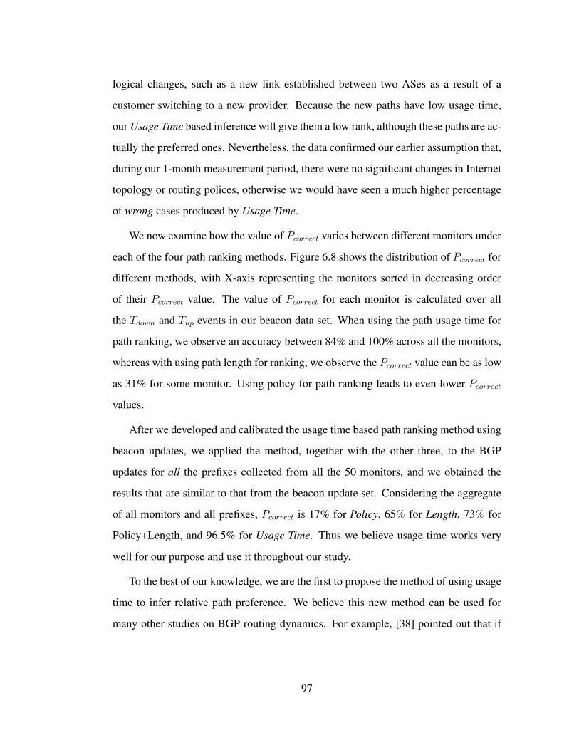
logical changes, such as a new link established between two ASes as a result of a

customer switching to a new provider. Because the new paths have low usage time,

our Usage Time based inference will give them a low rank, although these paths are ac-

tually the preferred ones. Nevertheless, the data confirmed our earlier assumption that,

during our 1-month measurement period, there were no significant changes in Internet

topology or routing polices, otherwise we would have seen a much higher percentage

of wrong cases produced by Usage Time.

We now examine how the value of Pcorrect varies between different monitors under

each of the four path ranking methods. Figure 6.8 shows the distribution of Pcorrect for

different methods, with X-axis representing the monitors sorted in decreasing order

of their Pcorrect value. The value of Pcorrect for each monitor is calculated over all

the Tdown and Tup events in our beacon data set. When using the path usage time for

path ranking, we observe an accuracy between 84% and 100% across all the monitors,

whereas with using path length for ranking, we observe the Pcorrect value can be as low

as 31% for some monitor. Using policy for path ranking leads to even lower Pcorrect

values.

After we developed and calibrated the usage time based path ranking method using

beacon updates, we applied the method, together with the other three, to the BGP

updates for all the prefixes collected from all the 50 monitors, and we obtained the

results that are similar to that from the beacon update set. Considering the aggregate

of all monitors and all prefixes, Pcorrect is 17% for Policy, 65% for Length, 73% for

Policy+Length, and 96.5% for Usage Time. Thus we believe usage time works very

well for our purpose and use it throughout our study.

To the best of our knowledge, we are the first to propose the method of using usage

time to infer relative path preference. We believe this new method can be used for

many other studies on BGP routing dynamics. For example, [38] pointed out that if

97

after a routing event, the stable path is switched from P1 to P2, the root cause of the

event should lie on the better path of the two. The study used length-only in their path

ranking and the root cause inference algorithm produced a mixed result. Our result

shows that using length for path ranking gives only about 65% accuracy, and usage

time can give more than 96% accuracy. Using usage time to rank path can potentially

improve the results of the root cause inference scheme proposed in [38].

6.3 Characterizing Events

After applying the classification algorithm to BGP data, we count the number of Tdown

events observed by each monitor as a sanity check. A Tdown event means that a pre-

viously reachable prefix becomes unreachable, suggesting that the root cause of the

failure is very likely at the AS that originates the prefix, and should be observed by all

the monitors. Therefore, we expect every monitor to observe roughly the same number

of Tdown events. Figure 6.9 shows the number of Tdown events seen by each monitor.

Most monitors observe similar number of Tdown events, but there are also a few outliers

that observe either too many or too few Tdown events. Too many Tdown events can be

due to failures that are close to monitors and partition the monitors from the rest of the

Internet, or underestimation of the relative timeout T used to cluster updates. Too few

Tdown events can be due to missing data during monitor downtime, or overestimation

of the relative timeout T . In order to keep consistency among all monitors, we decided

to exclude the head and tail of the distribution, reducing the data set to 32 monitors.

Now we examine the results of event classification. Tables 6.1 and 6.2 show the

statistics for January and February respectively for each event class, including the total

number of events, the average event duration, the average number of updates per event,

and the average number of unique paths explored per event. We exclude Tequal events

from the table since their percentage is negligible. Comparing the results from the two

98

0

200000

400000

600000

800000

1e+06

1.2e+06

0 5 10 15 20 25 30 35 40 45

Num

ber

of T

dow

n ev

ents

Monitor ID

Figure 6.9: Number of Tdown events per monitor.

No. of Events Duration No. of No. of

(×106) (second) Updates Paths

Tup 3.39 45.26 2.30 1.59

Tdown 3.35 116.34 4.10 1.95

Tshort 7.37 31.32 1.71 1.27

Tlong 8.04 69.93 2.52 1.62

Tpdist 15.51 174.19 4.66 2.33

Tspath 23.24 38.91 1.52 1.00

Table 6.1: Event Statistics for Jan 2006 (31 days)

99

No. of Events Duration No. of No. of

(×106) (second) Updates Paths

Tup 2.88 42.54 2.20 1.54

Tdown 2.85 118.98 4.00 1.90

Tshort 8.09 39.68 2.46 1.51

Tlong 8.94 67.26 2.51 1.70

Tpdist 16.01 190.79 4.80 2.31

Tspath 20.44 30.42 1.44 1

Table 6.2: Event Statistics for Feb 2006 (28 days)

0

0.1

0.2

0.3

0.4

0.5

0.6

0.7

0.8

0.9

1

0 50 100 150 200 250 300

Fre

quen

cy (

CD

F)

Event duration (s)

TupTdownTshortTlongTpdist

Figure 6.10: Duration of events for January

2006.

0

0.1

0.2

0.3

0.4

0.5

0.6

0.7

0.8

0.9

1

0 50 100 150 200 250 300

Fre

quen

cy (

CD

F)

Event duration (s)


Figure 6.11: Duration of events for Febru-

ary 2006.

100

0

0.1

0.2

0.3

0.4

0.5

0.6

0.7

0.8

0.9

1

1 2 3 4 5 6

Fre

quen

cy (

CD

F)

Number of updates per event


Figure 6.12: Number of Updates per Event,

January 2006.

0

0.1

0.2

0.3

0.4

0.5

0.6

0.7

0.8

0.9

1

0 1 2 3 4

Fre

quen

cy (

CD

F)

Number of ASPATHs explored per event


Figure 6.13: Number of Unique Paths Ex-

plored per Event, January 2006.

0

0.1

0.2

0.3

0.4

0.5

0.6

0.7

0.8

0.9

1

0 50 100 150 200 250 300

Fre

quen

cy (

CD

F)

Event duration (s)


Figure 6.14: Duration of events for unsta-

ble prefixes, January 2006.

0

0.1

0.2

0.3

0.4

0.5

0.6

0.7

0.8

0.9

1

0 50 100 150 200 250 300

Fre

quen

cy (

CD

F)

Event duration (s)


Figure 6.15: Duration of events for stable

prefixes, January 2006.

101

months, we note that the values are very close, as can also be observed by comparing

the distribution of event duration on Figures 6.10 and 6.11. Given this similarity, we

will base our following analysis on January data, although the same observations apply

to February.

There are three observations. First, the three high-level event categories in Figure

6.4 have approximately the same number of events: Path-Change events are about 36%

of all the events, Same-Path 34% and Path-Disturbance 30%. Breaking down Path-

Change events, we see that the number of Tdown balances that of Tup, and the number

of Tlong balances that of Tshort. This makes sense since Tdown failures are recovered

with Tup events, and Tlong failures are recovered with Tshort events.

Second, the average duration of different types of events can be ordered as follows:

Tshort < Tspath ' Tup < Tlong � Tdown < Tpdist4. Figure 6.10 shows the distributions

of event durations, 5 which also follow the same order. Note that the shape of the curves

is stepwise with jumps at multiples of around 26.5 seconds. The next section will

explain that this is due to the MinRouteAdvertisementInterval (MRAI) timer, which

controls the interval between consecutive updates sent by a router. The default range

of MRAI timer has the average value of 26.5 seconds, making events last for multiples

of this value. Table 6.1 also shows that Tpdist events have the longest duration, the most

updates and explore the most unique paths. This suggests that Tpdist likely contains two

events very close in time, e.g., a link failure followed shortly by its recovery. A study

[65] on network failures inside a tier-1 provider revealed that about 90% of the failures

on high-failure links take less that 3 minutes to recover, while 50% of optical-related

failures take less than 3.5 minutes to recover. Therefore there are many short-lived

network failures and they can very well generate routing events like Tpdist. On the

4The order of Tspath and Tshort average durations invert on February 2006, even though the valuesremain very close to each other.

5The Tspath curve is omitted from the figure for clarity.

102

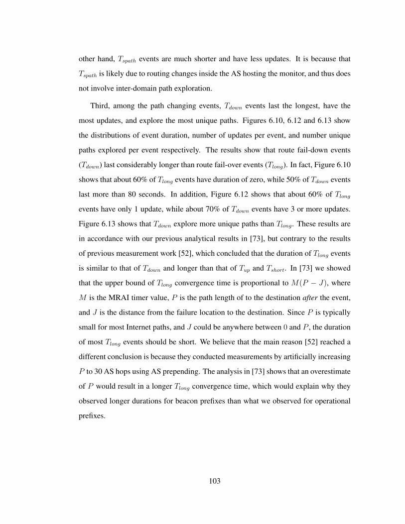
other hand, Tspath events are much shorter and have less updates. It is because that

Tspath is likely due to routing changes inside the AS hosting the monitor, and thus does

not involve inter-domain path exploration.

Third, among the path changing events, Tdown events last the longest, have the

most updates, and explore the most unique paths. Figures 6.10, 6.12 and 6.13 show

the distributions of event duration, number of updates per event, and number unique

paths explored per event respectively. The results show that route fail-down events

(Tdown) last considerably longer than route fail-over events (Tlong). In fact, Figure 6.10

shows that about 60% of Tlong events have duration of zero, while 50% of Tdown events

last more than 80 seconds. In addition, Figure 6.12 shows that about 60% of Tlong

events have only 1 update, while about 70% of Tdown events have 3 or more updates.

Figure 6.13 shows that Tdown explore more unique paths than Tlong. These results are

in accordance with our previous analytical results in [73], but contrary to the results

of previous measurement work [52], which concluded that the duration of Tlong events

is similar to that of Tdown and longer than that of Tup and Tshort. In [73] we showed

that the upper bound of Tlong convergence time is proportional to M(P − J), where

M is the MRAI timer value, P is the path length of to the destination after the event,

and J is the distance from the failure location to the destination. Since P is typically

small for most Internet paths, and J could be anywhere between 0 and P , the duration

of most Tlong events should be short. We believe that the main reason [52] reached a

different conclusion is because they conducted measurements by artificially increasing

P to 30 AS hops using AS prepending. The analysis in [73] shows that an overestimate

of P would result in a longer Tlong convergence time, which would explain why they

observed longer durations for beacon prefixes than what we observed for operational

prefixes.

103

6.3.1 The Impact of Unstable Prefixes

So far we have been treating all destination prefixes in the same way by aggregating

them in a single set in our measurements. However, previous work[79] showed that

most of routing instabilities affect a small number of unstable prefixes, and popular

destinations (with high traffic volume) are usually stable. Therefore, it might be the

case that the results we just described are biased towards those unstable prefixes, since

these prefixes are associated with more events. In order to verify if this is the case, we

classify each prefix p into one of two classes, based on the number of events associated

with it. If we let E be the median of the distribution of the number of events per prefix

E(p), then we can classify each prefix p in: (1) unstable if E(p) ≥ E, or (2) stable if

E(p) < E. From the 205,980 prefixes in our set, only 28,954 (or 14%) were classified

as unstable, i.e. 14% of prefixes were responsible for 50% of events. In Figures 6.14

and 6.15 we show the distribution of event duration for unstable and stable prefixes

respectively. Note that not only are these two distributions very similar, but they are

also very close to the original distribution of the aggregate in Figure 6.10. Based on

these observations, we believe there is no sensitive bias in the aggregated results shown

before.

6.4 Policies, Topology and Routing Convergence

In this section we compare the extent of slow convergence across different prefixes

and different monitors to examine the impacts of routing polices and topology on slow

convergence.

104

6.4.1 MRAI Timer

In order to make fair comparisons of slow convergence observed by different monitors,

we need to be able to tell whether a monitor enables MRAI timer or not. The BGP

specification (RFC 4271 [78]) defines the MinRouteAdvertisementInterval (MRAI) as

the minimum amount of time that must elapse between two consecutive updates sent

by a router regarding the same destination prefix. Lacking MRAI timer may lead to

significantly more update messages and longer global convergence time [40]. Even

though it is a recommended practice to enable the MRAI timer, not all routers are

configured this way. Since MRAI timer will affect observed event duration and number

of updates, for the purpose of studying impacts of policies and topology, we should

only make comparisons among MRAI monitors, or among non-MRAI monitors, but

not between MRAI and non-MRAI monitors.

By default the MRAI timer is set to 30 seconds plus a jitter to avoid unwanted

synchronization. The amount of jitter is determined by multiplying the base value

(e.g., 30 seconds) by a random factor which is uniformly distributed in the range [0.75,

1]. Assuming routers are configured with the default MRAI values, we should (1) not

observe consecutive updates spaced by less than 30 × 0.75 = 22.5 seconds for the

same destination prefix, and (2) observe a considerable amount of inter-arrival times

between 22.5 and 30 seconds, centered around the expected value, 30× 0.75+12

= 26.5

seconds.

For each monitor, we define a Non-MRAI Likelihood, LM , as the probability of

finding consecutive updates for the same prefix spaced by less than 22 seconds. Figure

6.16 shows LM for all the 50 monitors in our initial set. Clearly, there are monitors

with very high LM and monitors with very small LM . The curve has a sharp turn,

hinting a major configuration change. Based on this, we decided to set LM = 0.05 as

a threshold to differentiate MRAI and non-MRAI monitors. Those with LM < 0.05

105

0

0.1

0.2

0.3

0.4

0.5

0.6

5 10 15 20 25 30 35 40 45 50

Pr

[inte

r-ar

rival

< x

sec

]Monitor ID

22 seconds10 seconds

Figure 6.16: Determining MRAI configuration.

are classified as MRAI monitors, and those with LM ≥ 0.05 are classified as non-

MRAI monitors. However, there could still be cases of non-MRAI monitors with

MRAI timer configuration just slightly bellow the RFC recommendation, and would

therefore be excluded using our method. In order to assure this was not the case, we

show in Figure 6.16 the curve corresponding to the probability of finding consecutive

updates spaced by less than 10 seconds. We note that the 10-second curve is very close

to the 22-second curve, and therefore we are effectively only excluding monitors that

depart significantly from the 30-second base value of the RFC.

Using this technique, we detect that 15 routers from the initial set of 50 are non-

MRAI (see the vertical line in Figure 6.16), and 10 of them are part of the set of 32

routers we used in previous section. We will use this set of 32-10=22 monitors for the

next subsection to compare the extent of slow convergence across monitors.

6.4.2 The Impact of Policy and Topology on Routing Convergence

Internet routing is policy-based. The “no-valley” policy [39], which is based on inter-

AS relationships, is the most prevalent one in practice. Generally, most ASes have rela-

tionships with their neighbors as provider-customer or peer-peer. In provider-customer

106

relationship, the customer AS pays the provider AS to get access service to the rest of

the Internet; in peer-peer relationship, the two ASes freely exchange traffic between

their respective customers. As a result, a customer AS does not forward packets be-

tween its two providers, and a peer-peer link can only be used for traffic between the

two incident ASes’ customers. For example, in Figure 6.19, paths [C E D], [C E F] and

[C B D] all violate the “no-valley” policy and generally are not allowed in the Internet.

Based on AS connectivity and relationships, the Internet routing infrastructure can

be viewed as a hierarchy.

• Core: consisting of a dozen or so tier-1 providers forming the top level of the

hierarchy.

• Middle: ASes that provide transit service but are not part of the core.

• Edge: stub ASes that do not provide transit service (they are customers only).

We collect an Internet AS topology [99], infer inter-AS relationships using the al-

gorithm from [94], and then classify all ASes into these three tiers. Core ASes are

manually selected based on their connectivity and relationships with other ASes [99];

Edge ASes are those that only appear at the end of AS paths; and the rest are middle

ASes. With this classification, we can locate monitors and prefix origins with regard

to the routing hierarchy.

Our set of 22 monitors consists of 4 monitors in the core, 15 in the middle and 3

at the edge. We would like to have a more representative set of monitors at the edge,

but we only found these many monitors in this class with consistent data from the

RouteViews and RIPE data archive. The results presented in this subsection might not

be quantitatively accurate due to the limitation of monitor set, but we believe they still

illustrate qualitatively the impact of monitor location on slow convergence.

107

In the previous section we showed that Tdown events have both the longest conver-

gence time and the most path exploration from all path change events. Furthermore,

in a Tdown event, the root cause of the failure is most likely inside the destination AS,

and thus all monitors should observe the same set of events. Therefore, the Tdown

events provide a common base for comparison across monitors and prefixes, and the

difference between convergence time and the number of updates should be most pro-

nounced. In this subsection we examine how the location of prefix origins and moni-

tors impact the extent of slow convergence.

Figure 6.17 shows the duration of Tdown events seen by monitors in each tier. The

order of convergence time is core < middle < edge, and the medians of convergence

times are 60, 84 and 84 seconds for core, middle and edge respectively. Taking into

account that our edge monitor ASes are well connected: one has 3 providers in the core

and the other two reach the core within two AS hops, we believe that in reality edge

will generally experience even longer convergence times than the values we measured.

Figure 6.18 shows that monitors in the middle and at the edge explore 2 or more paths

in about 60% of the cases, whereas monitors in the core explore at most one path in

about 65% of the cases.

In a Tdown event, the monitor will not finish the convergence process until it has

explored all alternative paths. Therefore, the event duration depends on the number of

alternative paths between the event origin and the monitor. In general, due to no-valley

policy [39], tier-1 ASes have fewer paths to explore than lower tier ASes. For example,

in Figure 6.19, node D (representing a tier-1 AS) has only one no-valley path to reach

node G (path 4), while node E has three paths to reach the same destination: paths 1,2

and 3. In order to reach a destination, tier-1 ASes can only utilize provider-customer

links and peer-peer links to other tier-1s, but a lower tier AS can also use customer-

provider links and peer-peer links in the middle tier, which leads to more alternative

108

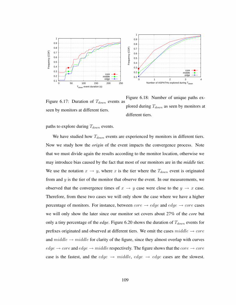
0.1

0.2

0.3

0.4

0.5

0.6

0.7

0.8

0.9

1

0 50 100 150 200 250

Fre

quen

cy (

CD

F)

Tdown event duration (s)

coremiddle

edge

Figure 6.17: Duration of Tdown events as

seen by monitors at different tiers.

0.1

0.2

0.3

0.4

0.5

0.6

0.7

0.8

0.9

1

0 1 2 3 4

Fre

quen

cy (

CD

F)

Number of ASPATHs explored during Tdown

coremiddle

edge

Figure 6.18: Number of unique paths ex-

plored during Tdown as seen by monitors at

different tiers.

paths to explore during Tdown events.

We have studied how Tdown events are experienced by monitors in different tiers.

Now we study how the origin of the event impacts the convergence process. Note

that we must divide again the results according to the monitor location, otherwise we

may introduce bias caused by the fact that most of our monitors are in the middle tier.

We use the notation x → y, where x is the tier where the Tdown event is originated

from and y is the tier of the monitor that observe the event. In our measurements, we

observed that the convergence times of x → y case were close to the y → x case.

Therefore, from these two cases we will only show the case where we have a higher

percentage of monitors. For instance, between core → edge and edge → core cases

we will only show the later since our monitor set covers about 27% of the core but

only a tiny percentage of the edge. Figure 6.20 shows the duration of Tdown events for

prefixes originated and observed at different tiers. We omit the cases middle → core

and middle → middle for clarity of the figure, since they almost overlap with curves

edge→ core and edge→ middle respectively. The figure shows that the core→ core

case is the fastest, and the edge → middle, edge → edge cases are the slowest.

109

Peer PeerProvider Customer

A B

C D

E F

G

CORE

MIDDLE

EDGE

1

2

3

4

Figure 6.19: Topology example.

0.1

0.2

0.3

0.4

0.5

0.6

0.7

0.8

0.9

1

0 50 100 150 200 250

Fre

quen

cy (

CD

F)

Tdown event duration (s)

core → coreedge → core

edge → middleedge → edge

Figure 6.20: Duration of Tdown events ob-

served and originated in different tiers.

0.1

0.2

0.3

0.4

0.5

0.6

0.7

0.8

0.9

1

0 1 2 3

Fre

quen

cy (

CD

F)

Number of paths explored during Tdown

core → coreedge → core

edge → middleedge → edge

Figure 6.21: Number of paths explored

during Tdown events observed and origi-

nated in different tiers.

Tdown duration (s)

core→core 54

middle→core 60

edge→core 61

middle→middle 83

edge→edge 85

edge→middle 87

Figure 6.22: Median of duration of Tdown

events observed and originated in different

tiers.

110

This observation is also confirmed by Figure 6.21, which shows the number of paths

explored during Tdown. Table 6.22 lists the median durations of Tdown events originated

and observed at different tiers. Events observed by the core have shortest durations,

which confirms our previous observation (Figure 6.17). Note that the edge → edge

convergence is slightly faster than the edge → middle convergence. We believe this

happens because, as mentioned before, our set of edge monitors are very close to

the core. Therefore, they may not observe so much path exploration as the middle

monitors, which may have a number of additional peer links to reach other edge nodes

without going through the core.

Note that we expect that the edge → edge case reflects most of the slow routing

convergence observed in the Internet because about 80% of the autonomous systems

in the Internet are at the edge, and about 68% of the Tdown events are originated at the

edge, as will be shown in the next subsection.

6.4.3 Origin of Fail-down Events

We will now examine where the Tdown events are originated in the Internet hierarchy.

Since we expect the set of Tdown events be common to all the 32 monitors of our data set

(section 6.3), we will use in this subsection a single monitor, the router 144.228.241.81

from Sprint. Note that similar results are obtained from other monitors.

Because our data set spans over 1 month period, we do not know if during this time

there was any high-impact event that triggered an abnormal number of Tdown failures,

which could bias our results if we simply use daily count or hourly count. Instead,

Figure 6.23 plots the cumulative number of Tdown events as observed by the monitor

during January 2006, and the time granularity is second. The cumulative number of

events grows linearly, with an approximate constant number of 3,600 Tdown events per

day. This uniform distribution along the time dimension seems also to suggest that

111

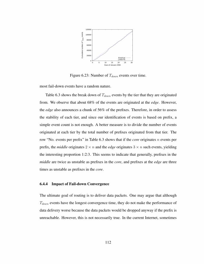
0

20000

40000

60000

80000

100000

120000

0 5 10 15 20 25 30

Cum

ulat

ive

num

ber

of T

dow

n ev

ents

Days of January 2006

EmpiricalLinear Fit

Figure 6.23: Number of Tdown events over time.

most fail-down events have a random nature.

Table 6.3 shows the break down of Tdown events by the tier that they are originated

from. We observe that about 68% of the events are originated at the edge. However,

the edge also announces a chunk of 56% of the prefixes. Therefore, in order to assess

the stability of each tier, and since our identification of events is based on prefix, a

simple event count is not enough. A better measure is to divide the number of events

originated at each tier by the total number of prefixes originated from that tier. The

row “No. events per prefix” in Table 6.3 shows that if the core originates n events per

prefix, the middle originates 2× n and the edge originates 3× n such events, yielding

the interesting proportion 1:2:3. This seems to indicate that generally, prefixes in the

middle are twice as unstable as prefixes in the core, and prefixes at the edge are three

times as unstable as prefixes in the core.

6.4.4 Impact of Fail-down Convergence

The ultimate goal of routing is to deliver data packets. One may argue that although

Tdown events have the longest convergence time, they do not make the performance of

data delivery worse because the data packets would be dropped anyway if the prefix is

unreachable. However, this is not necessarily true. In the current Internet, sometimes

112

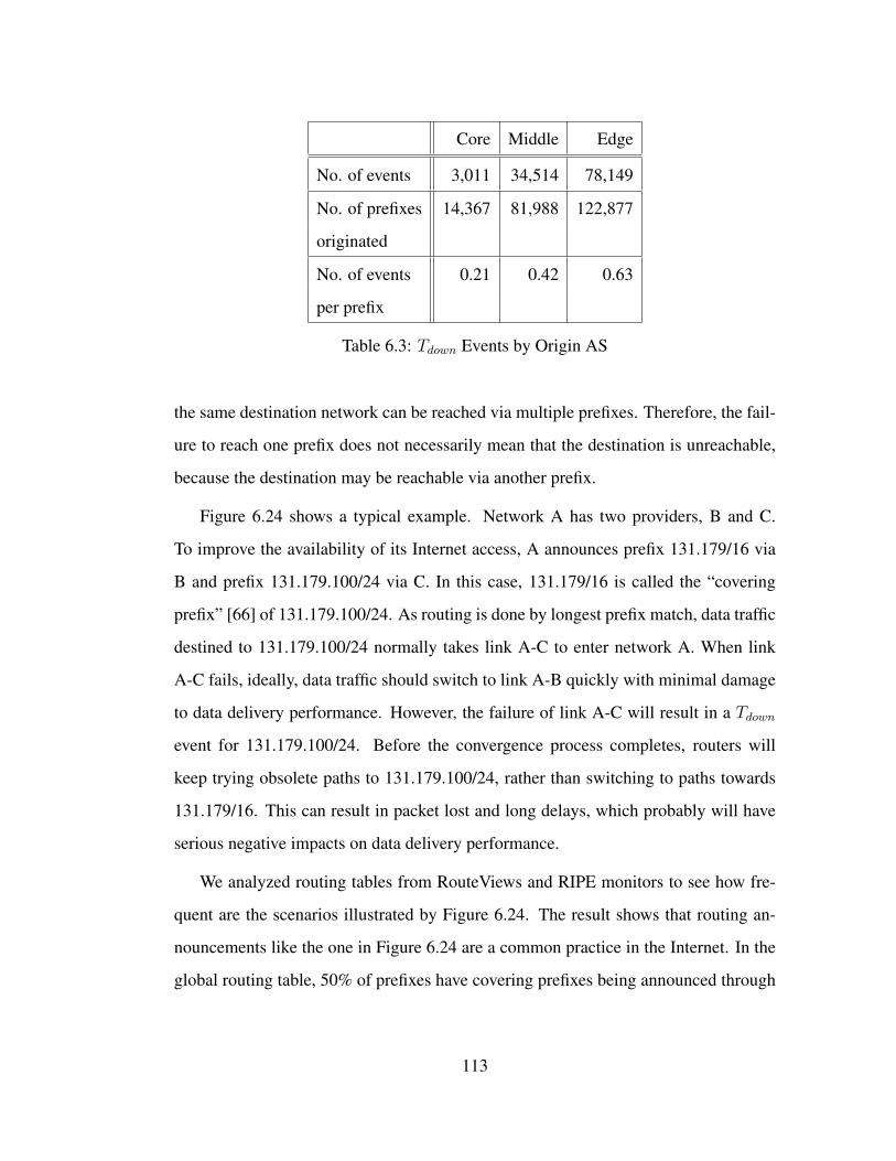
Core Middle Edge

No. of events 3,011 34,514 78,149

No. of prefixes 14,367 81,988 122,877

originated

No. of events 0.21 0.42 0.63

per prefix

Table 6.3: Tdown Events by Origin AS

the same destination network can be reached via multiple prefixes. Therefore, the fail-

ure to reach one prefix does not necessarily mean that the destination is unreachable,

because the destination may be reachable via another prefix.

Figure 6.24 shows a typical example. Network A has two providers, B and C.

To improve the availability of its Internet access, A announces prefix 131.179/16 via

B and prefix 131.179.100/24 via C. In this case, 131.179/16 is called the “covering

prefix” [66] of 131.179.100/24. As routing is done by longest prefix match, data traffic

destined to 131.179.100/24 normally takes link A-C to enter network A. When link

A-C fails, ideally, data traffic should switch to link A-B quickly with minimal damage

to data delivery performance. However, the failure of link A-C will result in a Tdown

event for 131.179.100/24. Before the convergence process completes, routers will

keep trying obsolete paths to 131.179.100/24, rather than switching to paths towards

131.179/16. This can result in packet lost and long delays, which probably will have

serious negative impacts on data delivery performance.

We analyzed routing tables from RouteViews and RIPE monitors to see how fre-

quent are the scenarios illustrated by Figure 6.24. The result shows that routing an-

nouncements like the one in Figure 6.24 are a common practice in the Internet. In the

global routing table, 50% of prefixes have covering prefixes being announced through

113

A

B C

131.179/16 131.179.100/24

X

Provider Customer

Figure 6.24: Case where Tdown convergence disrupts data delivery.

a different provider, and are therefore vulnerable to the negative impacts caused by

fail-down convergence. A recent study [47] showed that about 50% of VOIP glitches

as perceived by end users may be caused by BGP slow convergence.

114

CHAPTER 7

Prefix Hijacking and Internet Topology

In this chapter we study how different hijack attacks launched from very distinct places

in the network have different impact, and this impact depends on both the location of

the attacker and the location of the target network.

7.1 Prefix Hijacking

A prefix hijack occurs when an AS announces prefixes that it does not own. Now,

suppose AS-6 wrongly announces the prefix that belongs to AS-1, as shown in Figure

7.1. Note that AS-5 previously routed through AS-3 to reach AS-1. On receiving a

customer route through AS-6, it prefers the customer route over the peer route and

hence believes the false route. This is an example of a prefix hijack, in which a false

origin AS-6 announces a prefix it does not own, and deceives AS-5. In current routing

practice, it is difficult for an AS to differentiate between a true origin and a false origin.

Even though Internet Routing Registries (IRR) provide databases of prefix ownership,

the contents are not maintained up-to-date, and not all BGP routers are known to check

these databases. Hence, when presented multiple paths to reach the same prefix, a BGP

router will often choose the best path regardless of who originates this prefix, thus

allowing hijacked routes to propagate through the Internet. Prefix hijacks can be due to

malicious attacks or router mis-configurations. When legitimate data traffic is diverted

to the false origin, the data may be discarded, resulting in a traffic blackhole, or be

115

exploited for malicious purposes. A recent study [76] reported that some spammers

hijack prefixes in order to send spams without revealing their network identities.

The hijack depicted in Figure 7.1 is called a false origin prefix hijack, where an

AS announces the exact prefix owned by another AS. Another type of hijack, called

sub-prefix hijack, involves an AS announcing a more specific prefix (e.g. hijacker

announces a /24, when the true origin announces a /16). In this case, BGP routers will

usually treat them as different prefixes and maintain two separate entries in routing

tables. However, due to longest prefix matching in routing table lookups, data destined

to IP addresses in the /24 range will be forwarded to the false origin, instead of the true

origin. Prefix hijack can also involve a false AS link advertised in the AS path without

a change of origin. Our aim in this chapter is to understand that, how the topological

characteristics of two AS nodes announcing the same prefix influence the impact of

the hijack. Studying the impact of sub-prefix hijacks and false link hijacks involves

different considerations and is beyond the scope of this study. In the rest of this thesis,

we use the term prefix hijacks to refer to false origin prefix hijacks. We call the AS

announcing a prefix it does not own as the false origin, and the AS whose prefix is

being attacked as the true origin. Upon receiving the routes from both the false origin

as well as the true origin, an AS that believes the false origin is said to be deceived,

while an AS that still routes to the true origin is said to be unaffected.

7.2 Hijack Evaluation Metrics

For our simulations, we model the Internet topology as a graph, in which each node

represents an AS, and each link represents a logical relationship between two neighbor-

ing AS nodes. Note, two neighboring odes may have multiple physical links between

themselves. However, BGP paths are represented in the form of AS AS links, and

hence we abstract connections between two AS nodes as a single logical link. For

116

4

2

1

3

6

5

Provider CustomerPeer Peer

1

1

Tier-1

True origin False origin

1

Figure 7.1: Hijack scenario.

simplicity, each node owns exactly one unique prefix, i.e. no two nodes announce the

same prefix except during hijack. A prefix hijack at any given time involves only one

hijacker, and the hijacker can target only one node.

To capture the interaction between the entities involved in a hijack, we introduce a

variable β(a, t, v), function of false origin a, true origin t and node v as follows:

β(a, t, v) =

1 : if node v is deceived by false

origin a for true origin t’s prefix

0 : otherwise

(7.1)

Due to the rich connectivity in Internet topology, a node often has multiple equally

good paths to reach the same prefix. Figure 7.1 shows a case where AS-4 has three

equally good paths to reach the same prefix, two to the true origin AS-1 (through AS-2

and AS-3), and one to the false origin AS-6. In our model, we assume a node will

break the tie randomly. Therefore, we define the expected value of β as follows. Let

p(v, n) be the number of equally preferred paths (e.g. same policy, same path length)

from the node v to node n. E.g., in Figure 7.1, p(4, 1) = 2 since AS-4 has two paths

via AS-2 and AS-3 to reach AS-1, and p(4, 6) = 1 since AS-4 has only one route via

AS-5 to reach AS-6. If nodes use random tie-break to decide between multiple equally

117

good preferred paths, then the expected value for β is defined as:

β(a, t, v) =p(v, a)

p(v, a) + p(v, t)(7.2)

yielding β(6, 1, 4) = 13

for the example in the figure. β is the probability of a node v

being deceived by a given false origin a announcing a route belonging to true origin t.

Impact

We use the term impact to measure the attacking power of a node launching prefix

hijacks. We define impact of a node a as the fraction of the nodes that believe the false

origin a during an attack on true origin t. More formally, the impact of a node a is

given by:

I(a) =∑t∈N

∑v∈N

β(a, t, v)

(N − 1)(N − 2)(7.3)

Note that the outer sum is over N −1 true origins (we exclude the false origin) and the

inner sum is over N − 2 nodes (excluding both the false origin and true origin).

Resilience

We use the term resilience to measure the defensive power of a node against hijacks

launched against its prefix. We define the resilience of a node t as the fraction of nodes

that believe the true origin t given an arbritary hijack against t. More formally, the

node resilience R(t) of a node t is given by:

R(t) =∑a∈N

∑v∈N

β(t, a, v)

(N − 1)(N − 2)(7.4)

Note, higher R(t) values indicate better resilience against hijacks, and higher I(a)

values indicate higher impact as an attacker.

118

Relation between Impact and Resilience

The true origin t and false origin a compete with each other to make nodes in the

Internet route to itself. For example in Figure 7.1, false origin AS-6 is hijacking a

prefix belonging to true origin AS-1. In this case, only AS-5 believes the false origin

and AS-4 has a 1/3 chance of being deceived. Therefore, the chances that a node

believes the false origin AS-6 when it hijacks AS-1 is given by 1+1/34

= 13.

Now if AS-1 was to hijack a prefix belonging to AS-6, then AS-5 would still believe

AS-6 and AS-4 will believe it with a probability of 1/3. Thus, in this case, the chances

that a node believes the true origin AS-6 when it is hijacked by AS-1 is 1+1/34

= 13.

We see that the resilience of the node as a true origin is equal to its impact as

a false origin. We note that in our model, when the roles of attacker and target are

switched, the impact of a node becomes its resilience. In the rest of the thesis, we

focus on resilience, while keeping in mind that a highly resilient node can also cause

high impact as a false origin.

7.3 Evaluating Hijacks

In this section, we aim to understand the topological resilience of nodes against prefix

hijacks by performing simulations on an Internet derived topology. We first explain

the simulation setup, followed by the main results of our simulation and the insight

behind the results.

7.3.1 Simulation Setup

For our simulations, we use an AS topology collected from BGP routing tables and

updates, representing a snapshot of the Internet as of Feb 15 2006 (available from

119

[98]). The details of how this topology was constructed are described in [99]. Our

topology consists of 22,467 AS nodes and 63,883 links. We assume each AS node

owns and announces a single prefix to its neighbors. We classify AS nodes into three

tiers: Tier-1 nodes, transit nodes, and stub nodes. To choose the set of Tier-1 nodes, we

started with a well known list, and added a few high degree nodes that form a clique

with the existing set. Nodes other than Tier-1s but provide transit service to other AS

nodes, are classified as transit nodes, and the remainder of nodes are classified as stub

nodes. This classification results in 8 Tier-1 nodes, 5,793 transit nodes, and 16,666 stub

nodes. We classify each link as either customer-provider or peer-peer using the PTE

algorithm[39] and use the no valley prefer customer routing policy to infer routing

paths (also used in previous works such as [95]). We abstracted the router decision

process into the following priorities (1)local policy based on relationship, (2)AS path

length, and (3)random tie-breaker.

Of the 22,467 AS nodes in our topology, we randomly picked 1,000 AS nodes

to represent false origins that would launch attacks on other AS nodes. We checked

the degree distribution of this set of 1,000 AS nodes, and found it to be similar to

the degree distribution of all the AS nodes. For each of the 22,467 AS nodes as a

true origin, we simulated a hijack with the 1,000 false origins. Thus we simulated

22, 467× 1, 000 ' 22.5 million hijack scenarios in total.

7.3.2 Characterizing Topological Resilience

Figure 7.2 shows the distribution of the resilience (average curve) for all the nodes

in our topology from our simulated hijacks. Since the resilience of each node results

from the average over 1,000 attackers, we also show the standard deviation range.

Note, higher values of resilience imply more resilience against hijacks.

This distribution shows that node resilience varies fairly linearly except at the two

120

0

0.2

0.4

0.6

0.8

1

0 5000 10000 15000 20000

Res

ilien

cy

Node ID

Average (µ)µ + σµ - σ

Figure 7.2: Distribution of node resilience.

0

0.1

0.2

0.3

0.4

0.5

0.6

0.7

0.8

0.9

1

0 0.1 0.2 0.3 0.4 0.5 0.6 0.7 0.8 0.9 1

Fre

quen

cy (

CD

F)

Node resiliency

Tier-1sTransits

Stubs

Figure 7.3: Resilience of nodes in different tiers.

extremes. Figure 7.2 also shows that the deviations at the two extremes are quite small

compared to the middle, indicating that some nodes(top left) are very resilient against

hijacks, while some others (bottom right) are easily attacked, regardless of the location

of the false origin.

As a first step in understanding how different nodes differ in their resilience, we

classify nodes into the three classes already described: tier-1, transit and stub and

plot the average resilience distribution (CDF) of each class of nodes in Figure 7.3. We

observe that the resilience distribution is very similar for transits and stubs, with transit

nodes being a little more resilient than stubs.

In contrast, tier-1 nodes show a very different distribution from the stubs and tran-

121

sits. From Figure 7.3 we observe that all the tier-1 nodes have an average resilience

value between 0.4 and 0.5. In addition, we note that about 40% of stubs and 55%

of transit nodes are more resilient than all tier-1 nodes. With tier-1 nodes being the

ones with the highest degree, it is surprising to see that close to 50% of the nodes

in the Internet are more resilient than tier-1s. Next, we explain why tier-1 nodes are

more vulnerable to hijacks than a lot of other nodes and generalize this explanation to

understand the characteristics impacting resilience.

7.3.3 Factors Affecting Resilience

We first understand the resilience of tier-1 nodes with a simple hijack scenario in Fig-

ure 7.4. AS-2, AS-3, AS-4 and AS-5 represent 4 tier-1 nodes inter-connected through

a peer-peer relationship. AS-1 and AS-6 are small ISPs connected to tier-1 AS nodes

through a customer-provider relationship. Finally AS-7 is a multi-homed customer of

AS-1 and AS-6. In Figure 7.4, AS-7 represents the false origin that hijacks a prefix

belonging to a tier-1 node, AS-4.

Recall in no-valley prefer customer policy, a customer route is preferred over a

peer route which in turn is preferred over a provider route. When AS-7 hijack’s AS-

4’s prefix and announces the false route to AS-1 and AS-6, both AS-1 and AS-6 prefer

the hijacked route over the genuine route to AS-4 since its a customer route. AS-1 in

turn announces the hijacked route to its tier-1 providers AS-2 and AS-3. These tier-1

AS nodes, AS-2 and AS-3 now have to choose between a customer route through AS-

1(hijacked route), and a peer route through AS-4 (genuine route). Again due to policy

preference, the tier-1 nodes will choose the customer route which happens to be the

hijacked route. Similarly, AS-5 will also choose the hijacked route. Once big ISPs like

tier-1 nodes are deceived by the hijacker, their huge customer base (many of whom are

single homed) are also deceived, thus causing a high impact. One can see from this

122

example, that the main reason for the low resilience in the case of a hijack on a tier-1

node is that tier-1 nodes inter-connect through peer-peer relationship thus rendering a

genuine route less preferred to other tier-1 nodes than hijacked routes from customers.

The key to high resilience is to make the tier-1 nodes and other big ISPs always

believe the true origin. The way to achieve this is to reach as many tier-1 nodes as

possible using a provider route. In addition, when a node has to choose between two

routes of the same preference, path length becomes a deciding factor, and thus the

shorter the number of hops to reach the tier-1 nodes, the better the resilience. From

our observations from simulation results, we found that the most resilient nodes are

direct customers of many tier-1 nodes and other big ISPs. As an example, in our

simulations, the node with highest resilience is a stub (AS-6432 DoubleClick) directly

connected to 6 tier-1 nodes, having a resilience value of 0.95. The nodes with lowest

resilience were single-home customers, connected to poorly connected providers.

To better understand the influence of tier-1 nodes, we classified the nodes in the

Internet based on the number of direct tier-1 providers. Figure 7.5 shows the distri-

bution of resilience for nodes with different connectivity to Tier-1. Note, the closer

the curve to the right hand side of the figure (x=1), the better the resilience of that set

of nodes. There are about 21,888 nodes with less than 3 connections to Tier-1, and

we observe in Figure 7.5 that these nodes are the least resilient. A total of 379 nodes

are directly connected to 3 Tier-1s and 104 nodes are connected to 4 Tier-1s. Only

88 nodes are connected to more than 4 Tier-1s, and these nodes prove to be the most

resilient, highlighting the role of connecting to multiple tier-1 nodes.

Summary: In this section, we used an Internet scale topology with no-valley prefer

customer policy routing to evaluate the resilience of nodes against random hijackers.

The key to achieve high resilience is to protect tier-1 nodes and other big ISPs from

being deceived by the hijacker. Our main result shows that the nodes that are direct

123

4

2

1

3

6

5

Provider CustomerPeer Peer

Tier-1

7False origin

True origin

4 4

4 4

4

Figure 7.4: Understanding resilience of tier-1 nodes

0

0.1

0.2

0.3

0.4

0.5

0.6

0.7

0.8

0.9

1

0 0.1 0.2 0.3 0.4 0.5 0.6 0.7 0.8 0.9 1

Fre

quen

cy (

CD

F)

Node resiliency

<3 Tier-1s=3 Tier-1s=4 Tier-1s>4 Tier-1s

Figure 7.5: Resilience of nodes with different number of Tier-1 providers.

124

customers of multiple tier-1 nodes are the most resilient to hijacks. On the other hand,

the tier-1 nodes themselves in spite of being so well connected, are much less resilient

to hijack. The next question we seek to answer in Section 7.4 is whether there is

evidence of such behavior in reality, where the routing decision process is much more

complex.

7.4 Prefix Hijack Incidents in the Internet

In this section we examine two hijack events, one from January 2006 which affected

a few tens of prefixes, and the other from December 2004 when over 100,000 prefixes

were hijacked. To gauge the impact of the prefix hijacks, we analyzed the BGP routing

data collected by the Oregon collector of the RouteViews project. The Oregon collec-

tor receives BGP updates from over 40 routers. These 40 routers belong to 35 different

AS nodes (a few AS nodes have more than one BGP monitor) and we consider an AS

as deceived by a hijack if at least one BGP monitor from that AS believes the hijacker.

We call these 35 AS nodes as monitors, as they provide BGP monitoring information

to the Oregon collector. The impact of a hijack is then gauged by the ratio of monitors

in the Internet that were deceived.

7.4.1 Case I: Prefix Hijacks by AS-27506

On January 22, 2006, AS-27506 announced a number of prefixes that did not belong

to it. This hijack incident was believed to be due to operational errors, and most of

the hijacked prefixes were former customers of AS-27506. We observed a total of

40 prefixes being hijacked by AS-27506. These 40 prefixes belonged to 22 unique

ASes. We present two representative prefixes; for the first prefix the false origin could

only deceive a small number of monitors, while for the second prefix the false origin

125

deceived the majority of the monitors. We examine the topological connectivity of the

true origins as compared to that of the false origin and the relation to the true origin’s

resiliency.

7.4.1.1 High Resiliency against Hijack

We examine a hijacked prefix that belongs to the true origin AS-20282. The impact

of hijacking this prefix is just over 10%, that is 4 out of the 35 monitored ASes were

deceived by the hijack. Figure 7.6(a) depicts the connectivity of some of the entities

involved in this hijack incident. The nodes colored in gray are the nodes deceived by

the false origin AS-27506, and the white nodes persisted with the true origin. The

true origin AS-20282 is a direct customer of two tier-1 nodes, AS-701 and AS-3356.

Before the hijack incident, all the 35 monitors used routes containing one of these two

tier-1 ASes as the last hop in the AS path to reach the prefix. The hijacker AS-27506

is a customer of AS-2914, another tier-1 node. When AS-27506 hijacked the prefix,

AS-2914 chose the false customer route from AS-27506 over an existing peer route

through AS-701. The false route was further announced by AS-2914 to other tier-1

peers including AS-701 and AS-3356, however neither of them adopted the new route

because they chose the customer route announced by the true origin AS-20282. Other

tier-1 ASes, such as AS-1239 (not shown in the figure), did not adopt to the false route

from AS-2914 either, most likely because the newly announced false route was 2 hops

in length, the same as that of their existing route through AS-701 or AS-3356, and

the recommended practice suggests to avoid unnecessary best path transitions between

equal external paths [36]. However we note that AS-3130, who is a customer of both

a deceived and an unaffected tier-1 providers, also got deceived, possibly because the

new path {2914, 27506} is shorter than the original path which contained 3 AS hops.

126

701 2914

3356

20282 3130

Tier-1

PeerPeerProvider Customer

true Origin

27506

false origin

(a) High resiliency: Tier-1 provider

2914 preferred the customer route to

false origin 27506 instead of the peer

route. Similarly tier-1 providers 701

and 3356 stayed with their customer

routes to the true origin 20282. Other

tier-1 providers like X received a peer

route to false origin that is no bet-

ter than existing route and did not

change route. 3130 routed to the false

origin since the route via one of its

providers, 2914, was shorter

2914

12006 3130

Tier-1


true Origin

27506

false origin

10910

23011

286

(b) Low resiliency: Tier-1 providers

like Y with a customer route to true

origin 23011 were not deceived by

false origin. Other tier-1 providers

like X received a shorter peer route

through 2914 and hence routed to

false origin. 286 preferred the shorter

route to 27506 via 2914 and was de-

ceived.

Figure 7.6: Case study: AS-27506 as false origin7.4.1.2 Low Resiliency against Hijack

Next, we examine another hijacked prefix which belonged to AS-23011. The average

impact of this hijacked prefix is 0.6, i.e. 21 out of the 35 monitors were deceived by

the hijack. Figure 7.6(b) shows the most relevant entities involved in this prefix hijack.

The true origin of this prefix was an indirect customer of 5 tier-1 ASes (not all of them

are shown in the figure) through its direct providers AS-12006 and AS-10910. The

connectivity of the hijacker is the same as before, and AS-2914 was deceived by the

hijack. The 5 tier-1 ASes on the provider path of the true origin stayed with the route

127

from the true origin AS-23011, however the rest of the tier-1 ASes were deceived this

time, possibly because the peer route to false origin through AS-2914 was shorter than

any other peer route to the true origin. AS-286 is a customer of the providers of both

the true and false origins, and it picked the false route through AS-2914 because it was

shorter. We note that, in this case, the true origin being indirect customers of multiple

tier-1 ASes ensured that those tier-1 ASes themselves did not get deceived, however

due to its longer distance to reach these tier-1 providers (compared to the true origin

in Figure 7.6(a)), other tier-1 ASes and their customers chose the shorter route to the

false origin.

One of the tier-1 providers that propagated the false route is known to verify the

origin of received routes with the Internet Routing Registries (IRR). However, it did not

block the hijack because the registry entries were outdated and still listed AS-27506

as an origin for the hijacked prefixes, and hence the hijack announcements passed the

registry check.

7.4.2 Case II: Prefix Hijacks by AS-9121

In this hijack incident, operational errors led AS-9121 to falsely announce routes to

over 100,000 prefixes on December 24, 2004. We use this case to evaluate the re-

siliency of tier-1 Ases as compared to that of direct customers of multiple tier-1 ASes.

Due to the large number of prefixes being falsely announced, some BGP protection

mechanisms such as prefix filters and maximum prefix limit, where an AS sets an up-

per limit on the number of routes a given neighbor may announce, were triggered and

made an effect on the overall impact. Given that multiple factors were involved in such

a large scale hijack event, it is difficult to accurately model the impact on an AS as a

function of its topological connectivity. Our objective in examining this case is to find

supporting evidence for our observations made in Section 7.3, as opposed to a detailed

128

study over all the hijacked prefixes. Similar to case-1, we observed how many moni-

tors were deceived for each hijacked prefix and used this result to gauge the resiliency

of the true origin AS.

7.4.2.1 Hijacked Tier-1 AS Prefix

In order to understand how tier-1 ASes fared against AS-9121 hijack, we studied the

impact of those hijacked prefixes that belonged to AS-7018, a tier-1 AS. Note that

AS-7018 announced over 1500 prefixes, and the impacts of different prefixes varied

noticeably, with around 7 to 8 monitors being deceived for most prefixes. For our case

study, we examine one of the hijacked prefixes which deceived the majority of the

monitors. Figure 7.7(a) shows the entities involved in the hijack of this tier-1 prefix.

The hijacker AS-9121 was connected to 3 providers, one of which was AS-1239,

a tier-1 AS. The true origin of the prefix in question was AS-7018, another tier-1 AS.

The grey nodes in the figure indicate those deceived by the hijack. All the 3 providers

of AS-9121, namely AS-1239, AS-6762, and AS-1299 were deceived into believing

the false origin. AS-1299 also propagated the false route to its tier-1 AS providers.

From our observations, a total of 19 out of 35 monitors were deceived by this hijack.

7.4.2.2 Hijacked Prefix belonging to Customer of Tier-1s

Next, we see how the AS-9121 hijack incident affected the prefixes belonging to an

AS that was a direct customer of multiple tier-1 ASes. We picked AS-6461 as an

example here because it connected to all the 8 tier-1 ASes. AS-6461 announced over

100 prefixes, 87 of which were hijacked by AS-9121. No more than 2 monitors were

deceived by the false origin of all the hijacked prefixes. Figure 7.7(b) shows the entities

involved in the hijack of one of the prefixes belonging to AS-6461. As before, AS-

6762 believed the false origin and was one of the monitors deceived of all the hijacked

129

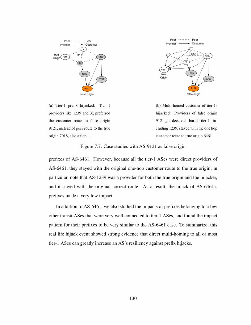
1239

6762

Tier-1


true Origin

9121

false origin

7018

Y

X

1299

(a) Tier-1 prefix hijacked: Tier 1

providers like 1239 and X, preferred

the customer route to false origin

9121, instead of peer route to the true

origin 7018, also a tier-1.

1239

6762

Tier-1


true Origin

9121

false origin

X

12996461

(b) Multi-homed customer of tier-1s

hijacked: Providers of false origin

9121 got deceived, but all tier-1s in-

cluding 1239, stayed with the one hop

customer route to true origin 6461

Figure 7.7: Case studies with AS-9121 as false origin

prefixes of AS-6461. However, because all the tier-1 ASes were direct providers of

AS-6461, they stayed with the original one-hop customer route to the true origin; in

particular, note that AS-1239 was a provider for both the true origin and the hijacker,

and it stayed with the original correct route. As a result, the hijack of AS-6461’s

prefixes made a very low impact.

In addition to AS-6461, we also studied the impacts of prefixes belonging to a few

other transit ASes that were very well connected to tier-1 ASes, and found the impact

pattern for their prefixes to be very similar to the AS-6461 case. To summarize, this

real life hijack event showed strong evidence that direct multi-homing to all or most

tier-1 ASes can greatly increase an AS’s resiliency against prefix hijacks.

130

7.5 Discussion

It has been long recognized that prefix hijacking can be a serious security threat to the

Internet. Several hijack prevention solutions have been proposed, such as SBGP [46],

so-BGP [69], and more recently the effort in the IETF Secure Inter-Domain Routing

Working Group [16]. These proposed solutions use cryptographic-based origin au-

thentication mechanisms, which require coordinated efforts among a large number of

organizations and thus will take time to get deployed. Meanwhile prefix hijack inci-

dents occur from time to time and our work provides an assessment of the potential

impacts of these incidents. Several hijack detection systems have also been developed,

for example MyASN[80] and PHAS[54]. However since these systems are reactive in

nature, it is still important for network customers to understand the relations between

their networks’ topological connectivity and the potential vulnerability in face of prefix

hijacks.

Our simulation and analysis show that AS nodes with large node-degrees (e.g.,

tier-1 networks) are not the most resilient against hijacks of their own prefixes. An AS

can gain high resiliency against prefix hijacks by being direct or indirect customers

of multiple tier-1 providers with the shortest possible AS paths. Conversely, such

customer AS nodes can also make the most impact over the entire Internet, if they

inject false routes into the Internet. This finding suggests that securing the routing

announcements from the major ISPs alone is not effective in curbing a high impact

attack, and that it is even more important to watch the announcements from lower-tier

networks with good topological connectivity.

On the other hand, customer networks that are far away from their indirect tier-1

providers can be greatly affected if their prefixes get hijacked. These topologically

disadvantaged AS nodes are in the most need for investigating other means to pro-

tect themselves. Subscribing to prefix hijack detection systems, such as MyASN and

131

PHAS, would be helpful. To reduce the transient impact during the detection delay,

one may also look into another proposed solution called PGBGP [45], which is briefly

described in Section 8.

Note that the topological connectivity required for resiliency against prefix hijacks

is different from that required for fast routing convergence [71]. Fast convergence

benefits from fewer alternative paths when the routes change, thus prefixes announced

by tier-1 providers meet the requirement well; while hijack resiliency benefits from

being a direct or indirect customer of a large number of tier-1 providers, thus prefixes

are better hosted by well connected non-tier-1 AS nodes.

We would like to end this discussion by stressing the importance of understand-

ing prefix hijack impacts, even when the protection mechanisms are put in place. Our

evaluations on an Internet scale topology in Section 7.3 used a no-valley prefer cus-

tomer routing policy and showed that tier-1 AS nodes are not very resilient to hijacks

of their own prefixes since other tier-1 AS nodes prefer customer routes to false origin.

However, in reality a tier-1 AS may use various mechanisms, such as Internet Routing

Registries (IRR), to check the origin of a prefix before forwarding the route. Such

mechanisms would probably boost the resiliency of tier-1 AS nodes being hijacked.

On the other hand, these protection mechanisms can also fail or backfire, thus expos-

ing the vulnerability of a network. As we saw in case I of Section 7.4, most of the

hijacked prefixes were the former customers of the false origin AS and were recorded

in the Internet Routing Registry (IRR), which was not updated. Outdated registries

resulted in false routes being propagated to the rest of the Internet.

Another example of a protection mechanism is the maximum prefix filter in BGP

that allows an AS to configure the maximum number of routes received from a neigh-

bor. Thus, by limiting the total number of routes received from a neighbor, an AS

can limit the damage in case of the neighbor announcing false routes. In case II from

132

Section 7.4, AS-9121 announced over 100,000 false routes and one of its neighbors,

AS-1299, had a max prefix set to a relatively low value. AS-1299 believed only 1849

routes directly from AS-9121, but since the max prefix limit is per neighbor, AS-

1299 received hijacked routes from other neighbors as well. It learned a total of over

100,000 bad routes from all the neighbors combined, thus infecting a major portion

of its routing table [74]. These examples show how easily protection mechanisms can

fail due to human errors, underlining the need to understand the impact of hijacks in

face of protection failures, and the need to protect networks by multiple means such as

PGBGP and PHAS.

133

CHAPTER 8

Related Work

8.1 Internet Topology Modeling

Three main types of data sets have been available for AS-level topology inference: (1)

BGP tables and updates, (2) traceroute measurements, and (3) Internet Routing Reg-

istry (IRR) information. BGP tables and updates have been collected by the University

of Oregon RouteViews project [15] and by RIPE-RIS in Europe [14]. Traceroute-based

datasets have been gathered by CAIDA as part of the Skitter project [17], by an EU-

project called Dimes [82], and more recently by the iPlane project [57]. Other efforts

have extended the above measurements by including data from the Internet Routing

Registry [27, 83, 96]. However, studies that have critically relied on these topology

measurements have rarely examined the data quality in detail, thus the (in)sensitivity

of the results and claims to the known or suspected deficiencies in the measurements

has largely gone unnoticed.

Chang et al. [27, 30, 26] were among the first to study the completeness of com-

monly used BGP-derived topology maps; later studies [99, 77, 96], using different data

sources, yielded similar results confirming that 40% or more AS links may exist in the

actual Internet but are missed by the BGP-derived AS maps. He et al. [96] report an

additional 300% of peer links in IRR compared to those extracted from BGP data, how-

ever this percentage is likely inflated since they only took RIB snapshots from 35 of

the ∼700 routers providing BGP feeds to RouteViews and RIPE-RIS. All these efforts

134

have in common that they try to incrementally close the completeness gap, without first

quantifying the degree of (in)completeness of currently inferred AS maps. This thesis

relies on the ground truth of AS-level connectivity of different types of ASes to shed

light on what and how much is missing from the commonly-used AS maps and why.

Dimitropoulos et al. [34] use AS adjacencies as reported by several ISPs to validate an

AS relationship inference heuristic. They found that most links reported by ISPs that

are not in the public view are peer links. In contrast to their work, most of our findings

are inferred from iBGP tables, router configs, and syslog records collected over time

from thousands of routers. Our approach yields an accurate picture of the ground truth

as far as BGP adjacencies are concerned and allows us to verify precisely for each AS

link x, why x was missing from public view. Lastly, in view of the recent work [81]

that concludes that an estimated 700 route monitors would suffice to see 99.9% of all

AS-links, our approach shows that such an overall estimate comes with an important

qualifier: what is important is not the total number of monitors, but their locations

within the AS hierarchy. In fact, our findings suggest a simple strategy for placing

monitors to uncover the bulk of missing links, but unfortunately researchers have in

general little input when it comes to the actual placement of new monitors.

8.2 Path Exploration

There are two types of BGP update characterization work in the literature: passive

measurements [49, 50, 48, 90, 21, 58, 79, 93, 38], and active measurements [51, 52,

62]. The work presented in this thesis belongs to the first category. We conducted a

systematic measurement to classify routing instability events and quantify path explo-

ration for all the prefixes in the Internet. Our measurement also showed the impact of

AS’s tier level on the extent of path explorations.

Existing measurements of path exploration and slow convergence have all been

135

based on active measurements [51, 52, 62], where controlled events were injected into

the Internet from a small number of beacon sites. These measurement results demon-

strated the existence of BGP path exploration and slow convergence, but did not show

to what extent they exist on the Internet under real operational conditions. In contrast,

in this thesis we classify routing events of all prefixes, as opposed to a small number of

beacon sites, into different categories, and for each category we provide measurement

results on the updates per event and event durations. Given we examine the updates

from multiple peers for all the prefixes in the global routing table, we are able to iden-

tify the impact of AS tier levels on path exploration. Regarding the relation between

the tier levels of origin ASes, our results agree with previous active measurement work

[52] (using a small number of beacon sites) that prefixes originated from tier-1 ASes

tend to experience less slow convergence compared to prefixes originated from lower

tier ASes. Moreover, our results also showed that, for the same prefix, routers of dif-

ferent AS tiers observe different degree of slow convergence, with tier-1 ASes seeing

much less than lower tier ASes.

Existing passive measurements have studied the instability of all the prefixes. The

focuses have been on update inter-arrival time, event duration, and location of insta-

bility, and characterization of individual updates [49, 50, 48, 90, 21, 58, 79, 93, 38].

There is no previous work on classifying routing events according to their effects (e.g.

whether path becomes better or worse after the event). This thesis describe a novel path

preference heuristic based on path usage time, and studied in detail the characteristics

of different classes of instability events in the Internet.

Our approach shares certain similarity with [79, 93, 38] in that we all use a timeout-

based approach to group updates into events. Such an approach can mistakingly group

updates of multiple root causes that happened close to each other or overlapped in

time into a single event. As we discussed earlier, the events in our Path-Disturbance

136

category can be examples of grouping updates of overlap root causes, because the path

to a prefix changed at least twice, and often more times, during one event. We moved

a step forward by detecting and separating these overlapping events into a different

category. It is most likely that those Path-Change events with very long durations are

also overlapping events, and one possible way to identify them is to set a time threshold

on the event duration, which we plan to do in the future.

8.3 Prefix Hijacking

Previous efforts on prefix hijacking can be broadly sorted into two categories: hijack

prevention and hijack detection. Generally speaking, prefix hijack prevention solutions

are based on cryptographic authentications [86, 69, 46, 56, 84] where BGP routers

sign and verify the origin AS and AS path of each prefix. In addition to added router

workload, these solutions require changes to all router implementations, and some

of them also require a public key infrastructure. Due to these obstacles, none of the

proposed prevention schemes is expected to see deployment in near future.

A number of prefix hijack detection schemes have been developed recently [80, 54,

75, 45]. A commonality among these solutions is that they do not use cryptographic-

based mechanisms. In [75], any suspicious route announcements received by an AS

trigger verification probes to other AS nodes and the results are reported to the true

origin. In PGBGP [45], each router monitors the origin AS nodes in BGP announce-

ments for each prefix over time; any newly occurred origin AS of a prefix is considered

anomalous, and the router avoids using anomalous routes if the previously existing

route to the same prefix is still available. Different from the above en route detection

schemes, MyASN[80] is an offline prefix hijack alert service provided by RIPE. A

prefix owner registers the valid origin set for a prefix, and MyASN sends an alarm via

regular email when any invalid origin AS is observed in BGP routing updates. PHAS

137

[54] is also an off-path prefix hijack detection system which uses BGP routing data

collected by RouteViews and RIPE. Instead of asking prefix owners to register valid

origin AS sets as is done by MyASN, PHAS keeps track of the origin AS set for each

announced prefix, and sends hijack alerts via multiple path email delivery to the true

origin.

Unlike the prevention schemes, a hijack detection mechanism provides only half

of the solution: after a prefix hijack is detected, correction steps must follow. A recent

proposal called MIRO [95] gives end users the ability to perform correction after

detecting a problem. MIRO is a new inter-domain routing architecture that utilizes

multiple path routing. In MIRO, AS nodes can negotiate alternative routes to reach a

given destination, potentially bypassing nodes affected by hijack attacks.

The work presented in this thesis can be considered orthogonal to all the existing

efforts in the area. It examines the relation between an AS node’s topological con-

nectivity and its resiliency against false route attacks, or conversely, an AS node’s

topological connectivity and its impact as a launching pad for prefix hijacks.

138

CHAPTER 9

Conclusion

Assessing the quality of inferred AS-level Internet topology maps is an important and

difficult problem. There have been generally accepted notions that the public view

is good at capturing customer-provider links but may miss peering links. However,

there has been no systematic effort to provide hard evidence to either confirm or dis-

miss these notions. This thesis represents an important step towards addressing this

challenging problem. Recognizing that it is impractical to obtain a complete AS topol-

ogy through currently pursued data collection efforts, we approach the problem from

a new and different angle: obtaining the ground truth of sample ASes’ connectivity

structures and comparing them with the AS connectivity inferred from publicly avail-

able data sets. A key benefit we derive from this new way of tackling the problem is

that we gain a basic understanding of not only what parts of the actual topology may

be missing from the inferred ones, but also how severe the incompleteness problem

may be.

A critical aspect of our search for the ground truth of AS-level Internet connectivity

and of the proposed pragmatic approach to constructing realistic and viable AS maps

is that they both treat ASes not as generic nodes but as objects with a rich, important,

and diverse internal structure. Exploiting this structure is at the heart of this work. The

nature of this AS-internal structure permeates our definition of “ground truth” of AS-

level connectivity, our analysis of the available data sets in search of this ground truth,

our detailed understanding of the reasons behind and importance of the deficiencies

139

of commonly-used AS-level Internet topologies, and our proposed efforts to construct

realistic and viable maps of the Internet’s AS-level ecosystem. Faithfully account-

ing for this internal structure can also be expected to favor the constructions of AS

maps that withstand scrutiny by domain experts. Such constructions also stand a better

chance to represent fully functional and economically viable AS-level topologies than

models where the interconnections between different ASes are solely determined by

independent coin tosses. Validating the consistency of an approach to understanding

the AS-level Internet that utilizes the network-intrinsic meaning of what a node and

a link represents clearly requires extra efforts and creativity and will therefore feature

prominently in our future research efforts in this area.

The Internet is becoming flat, meaning the paths are becoming shorter and more

networks establish direct connectivity to avoid upstream costs and speed up content

delivery to customers. It’s important to understand the dependency between routing

protocol properties and this evolving trend. In this thesis we have studied two of these

properties: BGP path exploration and resiliency to prefix hijacks. As the connectivity

denseness of the network increases, we expect to see the values of path exploration to

increase as well, because there will be more possible paths to explore between lower

tier networks to reach other lower tier networks. On the other hand, our insights from

the prefix hijack analysis are particularly relevant to make connectivity recommenda-

tions to minimize the impact of prefix hijacks. In this case, the most resilient scenario

would be to connect directly to all the Tier-1 networks. We are currently developing

a solution to recover from hijack attacks based on this insight, and this is also part of

our future work.

140

REFERENCES

[1] AOL peering requirements. http://www.atdn.net/settlement free int.shtml.

[2] AT&T peering requirements. http://www.corp.att.com/peering/.

[3] CERNET BGP feeds. http://bgpview.6test.edu.cn/bgp-view/.

[4] European Internet exchange association. http://www.euro-ix.net.

[5] Geant2 looking glass. http://stats.geant2.net/lg/.

[6] Good practices in Internet exchange points.http://www.pch.net/resources/papers/ix-documentation-bcp/ix-documentation-bcp-v14en.pdf.

[7] Internet Routing Registry. http://www.irr.net/.

[8] Packet clearing house IXP directory. http://www.pch.net/ixpdir/Main.pl.

[9] PeeringDB website. http://www.peeringdb.com/.

[10] Personal Communication with Bill Woodcock@PCH.

[11] PSG Beacon List.

[12] Regional Internet Registry data. ftp://www.ripe.net/pub/stats.

[13] RIPE Beacon List.

[14] RIPE routing information service project. http://www.ripe.net/.

[15] RouteViews routing table archive. http://www.routeviews.org/.

[16] Secure Inter-Domain Routing (SIDR) Working Group.http://www1.ietf.org/html.charters/sidr-charter.html.

[17] Skitter AS adjacency list. http://www.caida.org/tools/measurement/skitter/as adjacencies.xml.

[18] Skitter destination list. http://www.caida.org/analysis/topology/macroscopic/list.xml.

[19] The Abilene Observatory Data Collections.http://abilene.internet2.edu/observatory/data-collections.html.

[20] Reka Albert and Albert-Laszlo Barabasi. Topology of evolving networks: localevents and universality. Physical Review Letters, 85(24):5234–5237, 2000.

141

[21] David Andersen, Nick Feamster, Steve Bauer, and Hari Balakrishnan. Topologyinference from bgp routing dynamics. In ACM SIGCOMM Internet Measure-ment Workshop (IMW), 2002.

[22] Hitesh Ballani, Paul Francis, and Xinyang Zhang. A study of prefix hijackingand interception in the Internet. In Proc. of ACM SIGCOMM, 2007.

[23] Albert-Laszlo Barabasi and Reka Albert. Emergence of scaling in random net-works. Science, 286(5439):509–512, 1999.

[24] T. Bu and D. Towsley. On distinguishing between Internet power law topologygenerators. In Proc. of IEEE INFOCOM, 2002.

[25] D. Chang, R. Govindan, and J. Heidemann. The temporal and topological char-acteristics of BGP path changes. In Proc. of the Int’l Conf. on Network Proto-cols (ICNP), November 2003.

[26] H. Chang. An Economic-Based Empirical Approach to Modeling the InternetInter-Domain Topology and Traffic Matrix. PhD thesis, University of Michigan,2006.

[27] H. Chang, R. Govindan, S. Jamin, S. J. Shenker, and W. Willinger. Towardscapturing representative AS-level Internet topologies. Elsevier Computer Net-works Journal, 2004.

[28] H. Chang, S. Jamin, and W. Willinger. Inferring AS-level Internet topologyfrom router-level path traces. In SPIE ITCom, 2001.

[29] H. Chang, S. Jamin, and W. Willinger. To peer or not to peer: modeling theevolution of the Internet’s AS-level topology. In Proc. of IEEE INFOCOM,2006.

[30] H. Chang and W. Willinger. Difficulties measuring the Internet’s AS-levelecosystem. In Annual Conference on Information Sciences and Systems(CISS’06), pages 1479–1483, 2006.

[31] Hyunseok Chang, Sugih Jamin, and Walter Willinger. Internet connectivity atthe AS-level: an optimization-driven modeling approach. In Proc ACM SIG-COMM MoMeTools workshop, 2003.

[32] Qian Chen, Hyunseok Chang, Ramesh Govindan, Sugih Jamin, Scott Shenker,and Walter Willinger. The origin of power-laws in Internet topologies revisited.In Proc. of IEEE INFOCOM, 2002.

142

[33] Brent Chun, David Culler, Timothy Roscoe, Andy Bavier, Larry Peterson,Mike Wawrzoniak, and Mic Bowman. Planetlab: an overlay testbed for broad-coverage services. ACM SIGCOMM Computer Comm. Review (CCR), 33(3):3–12, 2003.

[34] Xenofontas Dimitropoulos, Dmitri Krioukov, Marina Fomenkov, Bradley Huf-faker, Young Hyun, kc claffy, and George Riley. As relationships: inferenceand validation. ACM SIGCOMM Comput. Commun. Rev., 2007.

[35] Danny Dolev, Sugih Jamin, Osnat Mokryn, and Yuval Shavitt. Internet re-siliency to attacks and failures under bgp policy routing. Computer Networks,50(16):3183–3196, 2006.

[36] S. Sangli E. Chen. Avoid BGP Best Path Transitions from One Externalto Another. Internet Draft, IETF, June 2006. http://www.ietf.org/internet-drafts/draft-ietf-idr-avoid-transition-04.txt.

[37] M. Faloutsos, P. Faloutsos, and C. Faloutsos. On power-law relationships of theinternet topology. In Proc. of ACM SIGCOMM, 1999.

[38] Anja Feldmann, Olaf Maennel, Z. Morley Mao, Arthur Berger, and BruceMaggs. Locating internet routing instabilities. In Proc. of ACM SIGCOMM,2004.

[39] Lixin Gao. On inferring autonomous system relationships in the Internet.ACM/IEEE Transactions on Networking, 2001.

[40] Timothy G. Griffin and Brian J. Premore. An experimental analysis of bgpconvergence time. In Proc. of the Int’l Conf. on Network Protocols (ICNP),2001.

[41] B. Halabi and D. McPherson. Internet Routing Architectures. Cisco Press, 2ndedition, 2000.

[42] Benjamin Hummel and Sven Kosub. Acyclic type-of-relationship problems onthe internet: an experimental analysis. In ACM IMC, 2007.

[43] G. Huston. AS Number Consumption. The ISP Column, September 2005.

[44] Y. Hyun, A. Broido, and kc claffy. On third-party addresses in traceroute paths.In Proc. of Passive and Active Measurement Workshop (PAM), 2003.

[45] J. Karlin, S. Forrest, and J. Rexford. Pretty good bgp: Protecting bgp by cau-tiously selecting routes. Technical Report TR-CS-2005-37, University of NewMexico, Octber 2005.

143

[46] S. Kent, C. Lynn, and K. Seo. Secure Border Gateway Protocol. IEEE Journalof Selected Areas in Communications, 18(4), 2000.

[47] Nate Kushman, Srikanth Kandula, and Dina Katabi. Can you hear me now?!: itmust be BGP. SIGCOMM Comput. Commun. Rev., 37(2):75–84, 2007.

[48] C. Labovitz, A. Ahuja, and F. Jahanian. Experimental study of Internet stabilityand wide-area network failures. In Proceedings of FTCS99, June 1999.

[49] C. Labovitz, G. Malan, and F. Jahanian. Internet Routing Instability. In Proc. ofACM SIGCOMM, September 1997.

[50] C. Labovitz, R. Malan, and F. Jahanian. Origins of Internet routing instability.In Proc. of IEEE INFOCOM, 1999.

[51] Craig Labovitz, Abha Ahuja, Abhijit Abose, and Farnam Jahanian. Delayed In-ternet routing convergence. IEEE/ACM Transactions on Networking, 9(3):293– 306, June 2001.

[52] Craig Labovitz, Abha Ahuja, Roger Wattenhofer, and Srinivasan Venkatachary.The impact of Internet policy and topology on delayed routing convergence. InProc. of IEEE INFOCOM, April 2001.

[53] M. Lad, R. Oliveira, B. Zhang, and L. Zhang. Understanding the resiliency ofInternet topology against false origin attacks. In Proc. of IEEE DSN, 2007.

[54] Mohit Lad, Dan Massey, Dan Pei, Yiguo Wu, Beichuan Zhang, and LixiaZhang. PHAS: A prefix hijack alert system. In 15th USENIX Security Sym-posium, 2006.

[55] Lun Li, David Alderson, Walter Willinger, and John Doyle. A first-principlesapproach to understanding the Internet’s router-level topology. In Proc. of ACMSIGCOMM, 2004.

[56] S.W. Smith M. Zhao and D. Nicol. Aggregated path authentication for efficientbgp security. In 12th ACM Conference on Computer and Communications Se-curity (CCS), November 2005.

[57] H. Madhyastha, T. Isdal, M. Piatek, C. Dixon, T. Anderson, A. Krishnamurthy,and A. Venkataramani. iPlane: an information plane for distributed services. InProc. of OSDI, 2006.

[58] Olaf Maennel and Anja Feldmann. Realistic BGP traffic for test labs. InProc. of ACM SIGCOMM, 2002.

144

[59] Priya Mahadevan, Dimitri Krioukov, Kevin Fall, and Amin Vahdat. Systematictopology analysis and generation using degree correlations. In Proc. of ACMSIGCOMM, 2006.

[60] Priya Mahadevan, Dmitri Krioukov, Marina Fomenkov, Xenofontas Dim-itropoulos, k c claffy, and Amin Vahdat. The Internet AS-level topology: threedata sources and one definitive metric. ACM SIGCOMM Computer Comm. Re-view (CCR), 2006.

[61] R. Mahajan, D. Wetherall, and T. Anderson. Understanding BGP Misconfigu-ration. In In Proc. of ACM SIGCOMM, 2002.

[62] Z. Morley Mao, Randy Bush, Tim Griffin, and Matt Roughan. BGP beacons.In ACM SIGCOMM Internet Measurement Conference (IMC), 2003.

[63] Z. Morley Mao, Lili Qiu, Jia Wang, and Yin Zhang. On AS-level path inference.In Proc. SIGMETRICS, 2005.

[64] Zhuoqing Morley Mao, Jennifer Rexford, Jia Wang, and Randy H. Katz. To-wards an accurate AS-level traceroute tool. In Proc. of ACM SIGCOMM, 2003.

[65] Athina Markopoulou, Gianluca Iannaccone, Supratik Bhattacharyya, Chen-NeeChuah, and Christophe Diot. Characterization of failures in an IP backbone. InIEEE Infocom, Hong Kong, 2004.

[66] Xiaoqiao Meng, Zhiguo Xu, Beichuan Zhang, Geoff Huston, Songwu Lu, andLixia Zhang. IPv4 address allocation and BGP routing table evolution. In ACMSIGCOMM Computer Communication Review (CCR) special issue on InternetVital Statistics, Janurary 2005.

[67] Wolfgang Muhlbauer, Anja Feldmann, Olaf Maennel, Matthew Roughan, andSteve Uhlig. Building an AS-topology model that captures route diversity. InProc. of ACM SIGCOMM, 2006.

[68] Wolfgang Muhlbauer, Steve Uhlig, Bingjie Fu, Mickael Meulle, and Olaf Maen-nel. In search for an appropriate granularity to model routing policies. In Proc.of ACM SIGCOMM, 2007.

[69] J. Ng. Extensions to BGP to Support Secure Origin BGP. ftp://ftp-eng.cisco.com/sobgp/drafts/draft-ng-sobgp-bgp-extensions-02.txt, April 2004.

[70] Ricardo Oliveira, Dan Pei, Walter Willinger, Beichuan Zhang, and Lixia Zhang.In Search of the elusive Ground Truth: The Internet’s AS-level ConnectivityStructure. In Proc. ACM Sigmetrics, 2008.

145

[71] Ricardo Oliveira, Beichuan Zhang, Dan Pei, Rafit Izhak-Ratzin, and LixiaZhang. Quantifying Path Exploration in the Internet. In ACM Internet Mea-surement Conference (IMC), October 2006.

[72] Ricardo Oliveira, Beichuan Zhang, and Lixia Zhang. Observing the evolutionof Internet AS topology. In ACM SIGCOMM, 2007.

[73] Dan Pei, , Beichuan Zhang, Daniel Massey, and Lixia Zhang. An analysisof path-vector routing protocol convergence algorithms. Computer Networks,50(3):398 – 421, 2006.

[74] Alin C. Popescu, Brian J. Premore, and Todd Underwood. Anatomy of a leak:AS 9121. NANOG-34, May 2005.

[75] Sophie Qiu, Fabian Monrose, Andreas Terzis, and Patrick McDaniel. Efficienttechniques for detecting false origin advertisements in inter-domain routing. InSecond workshop on Secure Network Protocols (NPSec), 2006.

[76] Anirudh Ramachandran and Nick Feamster. Understanding the network-levelbehavior of spammers. In Proceedings of ACM SIGCOMM, 2006.

[77] Danny Raz and Rami Cohen. The Internet dark matter: on the missing links inthe AS connectivity map. In Proc. of IEEE INFOCOM, 2006.

[78] Y. Rekhter, T. Li, and S. Hares. Border Gateway Protocol 4. RFC 4271, InternetEngineering Task Force, January 2006.

[79] Jennifer Rexford, Jia Wang, Zhen Xiao, and Yin Zhang. BGP routing stabilityof popular destinations. In ACM SIGCOMM Internet Measurement Workshop(IMW), 2002.

[80] RIPE. Routing information service: myASn System.http://www.ris.ripe.net/myasn.html.

[81] Matthew Roughan, Simon Jonathan Tuke, and Olaf Maennel. Bigfoot,sasquatch, the yeti and other missing links: what we don’t know about the asgraph. In ACM IMC, 2008.

[82] Yuval Shavitt and Eran Shir. DIMES: Let the Internet measure itself. ACMSIGCOMM Computer Comm. Review (CCR), 2005.

[83] G. Siganos and M. Faloutsos. Analyzing BGP policies: Methodology and tool.In Proc. of IEEE INFOCOM, 2004.

[84] B. R. Smith, S. Murphy, and J. J. Garcia-Luna-Aceves. Securing the bordergateway routing protocol. In Global Internet’96, November 1996.

146

[85] L. Subramanian, S. Agarwal, J. Rexford, and R. Katz. Characterizing the inter-net hierarchy from multiple vantage points. In INFOCOM, 2002.

[86] L. Subramanian, V. Roth, I. Stoica, S. Shenker, and R. H. Katz. Listen andwhisper: Security mechanisms for bgp. In Proceedings of ACM NDSI 2004,March 2004.

[87] Lakshminarayanan Subramanian, Matthew Caesar, Cheng Tien Ee, Mark Han-dley, Morley Mao, Scott Shenker, and Ion Stoica. HLP: a next generation inter-domain routing protocol. In Proc. ACM SIGCOMM, 2005.

[88] W. B. Norton. The art of peering: the peering playbook, 2002.

[89] Lan Wang, Malleswari Saranu, Joel M. Gottlieb, and Dan Pei. UnderstandingBGP session failures in a large ISP. In Proc. of IEEE INFOCOM, 2007.

[90] Lan Wang, Xiaoliang Zhao, Dan Pei, Randy Bush, Daniel Massey, AllisonMankin, S. F. Wu, and Lixia Zhang. Observation and analysis of BGP behav-ior under stress. In ACM SIGCOMM Internet Measurement Workshop (IMW),2002.

[91] X. Wang and D. Loguinov. Wealth-based evolution model for the Internet AS-level topology. In Proc. of IEEE INFOCOM, 2006.

[92] J. Wu, Y. Zhang, Z. Mao, and K. Shin. Internet routing resilience to failures:analysis and implications. In Proc. of ACM CoNext, 2007.

[93] Jian Wu, Zhuoqing Morley Mao, Jennifer Rexford, and Jia Wang. Finding aneedle in a haystack: Pinpointing significant BGP routing changes in an IP net-work. In Symposium on Networked System Design and Implementation (NSDI),May 2005.

[94] Jianhong Xia and Lixin Gao. On the evaluation of AS relationship inferences.In Proc. of IEEE GLOBECOM, December 2004.

[95] Wen Xu and Jennifer Rexford. Miro: multi-path interdomain routing. In SIG-COMM, pages 171–182, 2006.

[96] Y. He, G. Siganos, M. Faloutsos, S. V. Krishnamurthy. A systematic frameworkfor unearthing the missing links: measurements and impact. In Proc. of NSDI,2007.

[97] Beichuan Zhang, Vamsi Kambhampati, Mohit Lad, Daniel Massey, and LixiaZhang. Identifying BGP Routing Table Transfers. In ACM SIGCOMM Miningthe Network Data (MineNet) Workshop, August 2005.

147

[98] Beichuan Zhang, Raymond Liu, Dan Massey, and Lixia Zhang. Internet Topol-ogy Project. http://irl.cs.ucla.edu/topology/.

[99] Beichuan Zhang, Raymond Liu, Daniel Massey, and Lixia Zhang. Collect-ing the Internet AS-level topology. ACM SIGCOMM Computer Comm. Review(CCR), 2005.

[100] Changxi Zheng, Lusheng Ji, Dan Pei, Jia Wang, and Paul Francis. A light-weight distributed scheme for detecting IP prefix hijacks in real-time. In Proc.of ACM SIGCOMM, 2007.

148

understanding the internet as-level structure

Documents