Understanding the Broad Institute’s GSEA and hands-on training with the software Presented by Alan E. Berger, Ph.D.

Lowe Family Genomics Core, School of Medicine, Johns Hopkins University

September 30, 2014 NIH Building 10 FAES Classroom 1

Loca

tions

of g

enes

in

1 g

ene

set

• Using gene sets, e.g., pathways, GO categories, to interpret microarray (and other) biology data• Using a measure of differential expression for all the genes, rather than a list of distinguished genes• The general approach of the Broad Institute’s GSEA software // comparison with DAVID (NIAID)• The statistics behind GSEA // The data files and formats required to use GSEA• Hands on running the GSEA software (using output data from Partek runs)• Understanding the output files produced by GSEA

The content of this set of slides is derived from several NIH-CIT tutorials on GSEA given by Aiguo Li, Ph.D., NIH-NCI and Alan Berger, Ph.D., in 2007 & 2008, and from slides prepared by Alan Berger and Maggie Cam, Ph.D., NIH-NCI for April and December 2013 NCI-BTEP classes on GSEA

my contact information:Alan E. Bergeraberger9@jhmi.edu410-550-5089

Outline• Functional Analysis of Microarray or RNA-seq Data – Analysis of

Differential Expression Between 2 groups at the Level of Gene Sets– Enrichment of gene sets in a list of “distinguished” genes (e.g., DAVID)– Gene set methods using all the available expression data – Broad Institute’s Gene Set Enrichment Analysis (GSEA)– How GSEA measures differential expression for each set of genes– Controlling effects of multiple comparisons in GSEA (False Discovery Rate (FDR))– The Broad Institute library of groups of gene sets (MSigDB)– What files are needed for GSEA and their required formats– User options and installing and running GSEA

• Hands-on running GSEA– Loading the required GSEA data files for an example cancer dataset– Using the GSEA GUI interface: Parameter selection– Rank-based analysis (submitting a measure of differential expression for each gene)– Understanding the GSEA outputs: judging statistical and biological significance

Background

• Genome-wide expression profiling with microarrays or RNA-sequencing has become an effective frequently used technique in molecular biology

• Interpreting the results to gain insights into biological mechanisms remains a major challenge

• For a typical two group comparison, e.g., tumor vs. normal, treated vs. control, a standard approach has been to produce a list of differentially expressed genes (DEGs)

• One also might obtain a list of “Distinguished Genes” from examining correlation of gene expression with a pertinent clinical variable, or from differences in methylation

Criteria for Differential Expression of a Gene

• Statistically significant differential expression – by t-test, multi-way ANOVA, etc.– P-value cut-off: require, e.g., p ≤ 0.01, but see FDR (which will

impose more stringent requirement for p-values)

• Satisfactory false discovery rate (FDR) – What fraction of the DEG list is false positives?– Benjamini-Hochberg procedure for estimating the FDR is a

common choice (e.g., require FDR ≤ 0.1 or 0.2).

• Sufficient level of fold change (FC)– require |FC| ≥ 1.5 or 2

(common convention: groups A, B, gene g with average expression levels A, B; FC A /B when A ≥ B ; FC -B /A when B ≥ A )

DEG lists II

• Large fraction of “Present” (above background) calls for the expression values in the group with the higher average expression level for that probe – 80% but require 3 out of 3 when group size = 3– If this is not satisfied for a given probe, do not do any statistical testing on

it. – This avoids false positives based on noise, and also reduces the number of

comparisons N used in calculating the FDR.– Can see very high correlations with a clinical variable with 0 Present calls

• Specific criteria and cutoffs depend on the platform, user preference and the biological situation (e.g., would like “reasonable amount” of mRNA and |FC| ≥ 2 for qRT-PCR verification)

Challenges in Interpreting Gene Microarray Data

• Even with DEG lists of upregulated and of down-regulated genes, still need to accurately extract valid biological inferences. Cutoff for inclusion in DEG lists is somewhat arbitrary.

• May obtain a long list of statistically significant genes without any obvious unifying biological theme

• May have few individual genes meeting the threshold for statistical significance

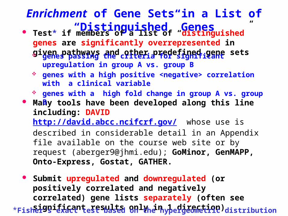
Enrichment of Gene Sets in a List of “Distinguished” Genes Test* if members of a list of “distinguished” genes are significantly

overrepresented in given pathways and other predefined gene sets

Many tools have been developed along this line including: DAVID http://david.abcc.ncifcrf.gov/ whose use is described in considerable detail in an Appendix file available on the course web site or by request (aberger9@jhmi.edu); GoMinor, GenMAPP, Onto-Express, Gostat, GATHER.

Submit upregulated and downregulated (or positively correlated and negatively correlated) gene lists separately (often see significant results only in 1 direction)

But note that Gene Set methods can only report enrichment for gene sets that are already in the library of gene sets being examined.

genes passing the criteria for significant upregulation in group A vs. group B genes with a high positive <negative> correlation with a clinical variable genes with a high fold change in group A vs. group B

*Fisher’s exact test based on the hypergeometric distribution along with FDR estimation

• 10,000 distinct genes in microarray platform

• 200 genes in the pathway S (2% of the genome).

• 50 genes in the “distinguished” list

• 6 genes of the distinguished gene list actually were in S

• One would expect on average to have 1 gene of a random list of 50 genes being in the pathway S.

• Here have 6 genes from the distinguished list in S. The hypergeometric distribution provides the p-value for this event (the probability that by chance one would have this many (6) or more genes of a randomly chosen list of 50 genes being in the pathway S). p = 0.00045

Example: gene list enriched in a gene set S

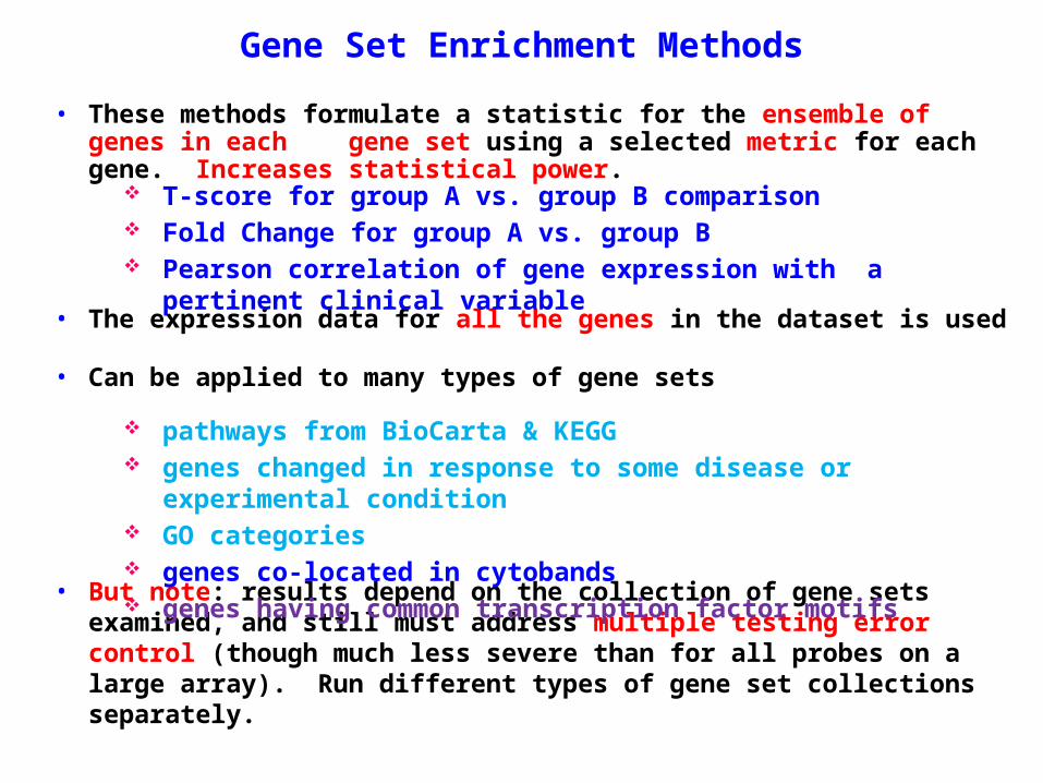
• These methods formulate a statistic for the ensemble of genes in each gene set using a selected metric for each gene. Increases statistical power.

• The expression data for all the genes in the dataset is used

• Can be applied to many types of gene sets

• But note: results depend on the collection of gene sets examined, and still must address multiple testing error control (though much less severe than for all probes on a large array). Run different types of gene set collections separately.

Gene Set Enrichment Methods

T-score for group A vs. group B comparison Fold Change for group A vs. group B Pearson correlation of gene expression with a pertinent clinical variable

pathways from BioCarta & KEGG genes changed in response to some disease or experimental condition GO categories genes co-located in cytobands genes having common transcription factor motifs

Some References for Gene Set Methods

1. Gene Set Enrichment Analysis (GSEA): Subramanian et al., A knowledge-based approach for interpreting genome-wide expression profiles, PNAS 2005, 102:15545; note Lamb et al., The Connectivity Map…, Science 2006, 313:1929. (see Broad Institute web page for this and other software)

2. PAGE: Parametric Analysis of Gene-Set Enrichment: Kim and Volsky, BMC Bioinformatics 2005, 6:144 (uses the average of the measure of differential expression (DE) of genes in a gene set, and values of DE over the chip to get a gene set z-score).

3. Systematic consideration of the issues in formulating and evaluating gene set methods: Ackermann and Strimmer, A general modular framework for gene set enrichment analysis, BMC Bioinformatics 2009, 10:47

4. Systematic consideration of the issues in formulating and evaluating gene set methods: Varemo, Nielsen and Nookaew, Enriching the gene set analysis of genome-wide data by incorporating directionality of gene expression and combining statistical hypotheses and methods, Nucleic Acids Research 2013 Mar 22 [Epub ahead of print]

GSEA Overview -- Workflow

GSEA is a computational method that determines whether an a priori

defined set of genes shows statistically significant, concordant

differences between two biological states (e.g. phenotypes).

text and figure from the Broad Institute web pages for GSEA : http://www.broad.mit.edu/gsea/index.html the current version of the figure at the Broad site is slightly different from the one above

The Broad Institute GSEA Documentation Main Page

The Broad GSEA web site has extensive information

Three Main Components in GSEA

Algorithm Software implementation (Broad Institute) Database of gene sets:

o Molecular signature database (MSigDB at the Broad Institute) containing collections of gene sets of interest

o Utilities mapping chip features to genes (e.g., Illumina or Affymetrix probe set IDs to HUGO gene symbols)

ES<0

Get ranked list L of all thegenes on the chip based on a chosen

measure, e.g., FC or Tscore, of the difference of

their expression levels between the phenotypes A & B under study, e.g., tumor vs. normal

Multiple hypothesis testing (MHT) error control for multiple S’s using

the estimated false discovery rate (FDR)

Analyze significance of this Kolmogorov-Smirnov

type statistic by permutation testing

For each gene set S:

find the location of each gene sin S within L

L

bands are locations in L of genes from S

+FC

-FC

ES>0

Generate enrichment score ES for S based

on running-sum statistic:“reward” presence of s

toward top or bottom of L

GSEA: Gene Set Enrichment Analysis

runn

ing

sum

L

ES(S) value of maximum deviation from 0 of the running sum

Enrichment Score (ES) Calculation

S = sum of fold changes for genes in gene set (S) (e.g., 100) N = no. of genes in the array (e.g., 1020)NH = no. of genes in the gene set (S) (e.g., 20)

Hits: Genes S +|FC| / Misses: Genes S -1/(N-NH)

Contribution to running sum for ES

Hits+|FC| /

Misses-1/(N-NH)

Running sum for ES

… … … …

Start with ranked list (L) of genes that are in (Hit) or not in (Miss) a gene set (S), using fold change (FC) as example metric

Hit +0.15 +0.15 0.15

Hit +0.12 +0.12 0.27

Miss -0.001 -0.001 0.269

Hit +0.09 +0.09 0.359

Hit +0.08 +0.08 0.439

Miss -0.001 -0.001 0.438

Ranked List(L)

15

12

10

9

8

6

FC

runn

ing

sum

L

The running enrichment score for a positive ES gene set from the P53 GSEA example data set

Zero crossing of ranking metric values

ES(S)

runn

ing

enric

hmen

t sc

ore

underlying running enrichment score figure copied from http://www.broadinstitute.org/gsea/datasets.jspp53 dataset (gene set is lairPathway)

+ -

locations of genes in S

p53 WT p53 MUT

The running enrichment score for a negative ES gene set from the P53 GSEA example data set

Zero crossing of ranking metric values

ES(S) ru

nnin

g en

richm

ent

scor

e

running enrichment score figure copied from http://www.broadinstitute.org/gsea/datasets.jspp53 dataset (gene set is BRCA_UP)

+ -

locations of genes in S

p53 WT p53 MUT

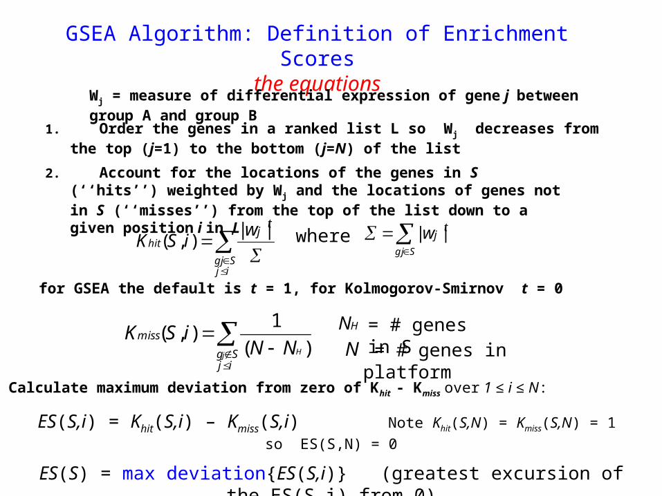
GSEA Algorithm: Definition of Enrichment Scoresthe equations

ES(S,i) = Khit(S,i) – Kmiss(S,i) Note Khit(S,N) = Kmiss(S,N) = 1 so ES(S,N) = 0

ES(S) = max deviation{ES(S,i)} (greatest excursion of the ES(S,i) from 0)

Wj = measure of differential expression of gene j between group A and group B

3. Calculate maximum deviation from zero of Khit - Kmiss over 1 ≤ i ≤ N:

ijSgj

hit

tjw

iSK||

),(

ijSg

miss

j HNNiSK

)(

1),(

for GSEA the default is t = 1, for Kolmogorov-Smirnov t = 0

HN = # genes in S = # genes in platformN

Sgj

tjw ||where

2. Account for the locations of the genes in S (‘‘hits’’) weighted by Wj and the locations of genes not in S (‘‘misses’’) from the top of the list down to a given position i in L

1. Order the genes in a ranked list L so Wj decreases from the top (j=1) to the bottom (j=N) of the list

If have at least 7 samples in each of the 2 groups, do sample label permutations to get statistics; otherwise

do gene set “permutations”

Gene Set PermutationFor a given gene set S (count of genes in S = s), each permutation is the random selection of s genes from all genes in the genome which have a probe on the platform, forming a random gene set S The corresponding enrichment score ES(S, ) = ES(S) is calculated from the original expression matrix using S

If ES(S) > 0, the resulting empirical p-value for S is the fraction of the ES(S, ) values that equal or exceed the actual enrichment score ES(S). The p-value is the fraction of time one would get an enrichment score ≥ ES(S)) just by random chance (estimated using the randomly sampled sets S) (and similarly for ES(S) < 0)

Testing the Significance of ES using Sample Label Permutations:

do 1000 sample label permutations * - for each permutation i randomly shuffle the labels of which sample is in which group while leaving the rest of the expression matrix fixed, and recalculate {DE(g)} and then the enrichment score for each S

perm

utati

on

num

ber

*actually want at least 7 samples in each group for sample label permutation, else do gene permutation

{ES(S,1)}{ES(S,2)}

{ES(S,4)}{ES(S,3)}

compute the differential expression value for each gene (DE(g)), and then the ES(S) values for all the gene sets

gene expression matrix, sample labels indicate phenotype group

Testing the Significance of ES

Significance of the observed ES(S) is compared with the set of empirical null distribution scores ES(S,) computed with the randomly assigned phenotypes or random gene sets.

G T1 T2 T3 T4 N1 N2 N3 N4

:1000 x

Histogram of 1000 ES(S,) Scores

ES(S,1)G T4 N3 N4 T3 T1 T2 N1 N2

G T3 N2 T1 N3 T4 N4 T2 N1

G N4 T4 N1 N3 T3 T4 N2 T1ES(S,2)ES(S,3)

:

ES(S,1000)

ES(S)

ESNULL(S):null distribution for ES(S)

ES(S)

The empirical, nominal p-value for each ES(S) is then calculated relative to the null distribution for ES(S): p = fraction of ES(S,) values ≥ ES(S)

How normalized enrichment scores (NES) are calculated from ES (using the NES helps normalize out effect of different gene set sizes)

mean{ES(S, ) values with the same sign as ES(S)}

original ES(S) NES(S)

Histogram of the ES(S,) values for a given S from the permutations

ES(S,)

mean{ES(S, ) values with the same sign as

ES(S, k)}

ES(S, k)

NES(S, k)

For each permutation and gene set S, compute NES(S, ) to use in computing the FDR:

ES(S)

ES(S,)

ES(S,1)

ES(S,3)ES(S,2)

GSEA returns two lists of gene sets: {S with NES > 0} and {S with NES < 0} (each sorted by NES value)

NES > 0, descending order

NES < 0, ascending order

If one has a list of the form A = {all gene sets S with NES(S) ≥ NES*}# with NES* a chosen value, one would like to estimate what fraction of the gene sets in A are false positives. This is called the False Discovery Rate (FDR) for A.

GSEA uses the collection {NES(S, k)} of NES values from the permutations as an empirical null distribution to estimate the FDR.

The {NES(S, k)} values estimate the pattern of NES values one would see if there was no difference between the 2 groups being examined.

Actual NES(S) values that “stand out” (are far enough out on a tail of the histogram of the {NES(S, k)} values) are considered to be true positives.

# and similarly for the case of all gene sets S with NES(S) ≤ NES* for some fixed value NES*

Histogram of NES(S, ) Scores

NES(S,)

NES*

NES(S,) ≥ NES*

False Discovery Rate (FDR) q value for each gene set S

Histogram of NES(S, ) Scores

NES(S,)

NES*

NES(S,) ≥ NES*F fraction of the positive NES(S,) ≥ NES*

Create a histogram of all NES(S, ), over all S and . Use this null distribution to compute an FDR q value for each NES(S) > 0* . Denote NES(S) by NES*FDR q value for S: D(S) = {gene sets with NES ≥ NES* }

estimate of # of false positives in D(S)

size of D(S) = # of S with NES(S) ≥ NES*

Histogram of NES(S) Scores

NES(S)

NES*

NES(S) ≥ NES*

NS+ # of gene sets with NES(S)

> 0

= F NS+ *

*similarly for NES(S) < 0

q

Dataset:

Wegener’s granulomatosis (WG)* vs. normal controls (C)41 patients, 23 controlsexpression data in PBMCs

* (now officially: granulomatosis with polyangiitis)

Example GSEA output

GSEA output: gene sets upregulated in WG

Gene set associated with immature neutrophils

note the WG dataset was from PBMCs

Note large number of genes in the gene set at the top of the complete ranked list (relative to gene set size)

DAVID output for WG dataset The collection of gene sets used in the run really matters