IFASD-2013-000

UNCERTAINTY QUANTIFICATION FOR LCO USING ANHARMONIC BALANCE METHOD

R. Hayes1 and S. Marques2

1r.hayes04@qub.ac.uk

2s.marques@qub.ac.ukSchool of Mechanical and Aerospace EngineeringQueen’s University Belfast, Belfast, UK, BT9 5AH

Keywords: flutter, optimization, stochastic, transonic.

Abstract: The harmonic balance method is an attractive solution for the computationof periodic flows and can be used as an alternative to classical time-marching methods,at a reduced computational cost. The current paper investigates using the HarmonicBalance (HB) method for LCO simulations under uncertainty. The HB formulation isused in conjuction with a non-intrusive polynomial-chaos (NIPC) approach to propagatevariability in parameters. Results show the potential of the HB approach together withNIPC to represent uncertainty in nonlinear dynamical systems at a fraction of the cost ofperforming time accurate simulations.

1 INTRODUCTION

As design complexity increases or new materials and novel technologies are introducedto new airframes, empirical methods become increasingly difficult to apply, hence a clearneed for physics based modeling tools has emerge. Aeroelasticity in particular is a goodillustration of this trend and a clear need for physics based modeling tools has beenidentified in [1]. Furthermore, predicting aeroelastic stability of an aircraft should alsoidentify the consequences of variability or uncertainty in model parameters, as discussedby Pettit [2]. In recent work, the authors investigated both these issues and demonstratedthe significant impact of structural variability on transonic flutter predictions [3,4]. Whennonlinearities are present, the amplitude of oscillation can become limited and originatinglimit cycle oscillations. This is also a problem of considerable practical interest and welldocumented for in-service aircraft [5, 6].

The presence of nonlinearities, either structural or aerodynamic, poses additional chal-lenges both in terms of complexity and computational resources. Two promising ap-proaches aimed at improving the efficiency of such simulations without compromisingthe underlying physics driving the oscillatory behaviour are: model reduction techniquesbased on the centre manifold theorem which has been applied to predict LCO on nonlin-ear structures [7]; harmonic balance (HB) based methods have also proven successful inpredicting LCO efficiently [6, 8], an overview for different variations of harmonic balancemethods, such as high-dimensional, incremental HB or elliptic HB method is given byDimitriadis [9].

As for flutter, LCO also proved to be sensitive to several parameters, which makes the useof stochastic tools attractive to this problem [7, 10–12]. In this work, a High-DimensionHarmonic Balance (HDHB) formulation is exploited to propagate variability in LCO sim-ulations, HDHB methods have been proved capable of representing the effects of non-linearities accurately and at a reduced cost; the impact of parametric variability is then

1

quantified using a Non-Intrusive Polynomial Chaos (NIPC) approach. The paper willsummarize the HDHB formulation adapted for 1 and 2 degrees of freedom dynamicalsystems, this is followed by the description of the probabilistic approach based on non-intrusive polynomial chaos expansions, which is capable of producing statistical outputdue to multiple parameter’s variability. The impact of variability on the responses ampli-tudes and motion frequency is assessed.

2 HARMONIC BALANCE FORMULATION

The harmonic balance formulation used in this work was proposed by Hall et al. [13]for time-periodic flow problems, this methodology was adapted to nonlinear dynamicalsystems by Liu et al. [14] and is summarize next. Consider a generic structural systemwhose behaviour can be described using a simple equation of motion given by:

Mx+Cx+Kx = F sin (ωt) (1)

where M, C, K, represent the mass, damping and stiffness of the system and F is anexternal force. The solution of (1) can be approximated to be a truncated Fourier seriesof NH harmonics with a fundamental frequency ω.

x(t) ≈ x0 +

NH∑

n=1

(x2n−1 cos(nωt) + x2n sin(nωt)) (2)

The first and second derivatives of x(t) with respect to time can be found to be:

x(t) ≈

NH∑

n=1

(−nωx2n−1 sin(nωt) + nωx2n cos(nωt)) (3)

x(t) ≈

NH∑

n=1

(−(nω)2x2n−1 cos(nωt)− (nω)2x2n sin(nωt)) (4)

By substituting these Fourier series back into (1) and collecting terms associated witheach harmonic a system of equations can be assembled to relate the dynamic propertiesto the Fourier coefficients. This algebraic system consists of 2NH+1 equations which canbe conveniently displayed in vector form.

(Mω2A2 +CωA+KI)X = F H (5)

where

X =

x0

x1

x2

x3...

x2NH

(2NH+1)×1

and H =

0010...0

(2NH+1)×1

Matrix A reconstructs the Fourier series from the harmonic balancing. Although im-plementing the classical Harmonic Balance approach is straightforward here, derivinganalytical solutions for the Fourier coefficients can be cumbersome or even impossible

2

for complex nonlinearities thus rendering the classical HB method inefficient for applica-tion to many practical problems [8]. The High Dimensional Harmonic Balance (HDHB)method overcomes these issues by casting the problem in the time domain where theFourier coefficients are related to 2NH + 1 equally spaced sub-time levels throughout onetemporal period using a constant transformation matrix which yields

X = EX and H = EH (6)

where:

X =

x(t0)x(t1)...

x(t2NH)

, H =

sin t0sin t1...

sin t2NH

, with ti =i2π

2NH + 1(i = 0, 1, 2, ..., 2NH)

Expressions for the transformation matrix E and its inverse E−1 which can be used torelate the time domain variables back to the Fourier coefficients ie. X = E−1X can befound in reference [14]. Using these transformation matrices system (6) can be cast in thetime domain.

(Mω2D2 +CωD+KI)X = F H (7)

where D = E−1AE. Equation (7) represents the HDHB system and can be solved usingeither pseudo-time marching or Newton-Raphson approaches. Two cases are studied inthis work, firstly a one degree of freedom Duffing oscillator and secondly a two degree offreedom pitch/plunge aerofoil with a cubic restoring force in pitch.

3 STOCHASTIC MODELING

The system of equations shown in (7), can be used to describe nonlinear time periodicdynamical systems; it also allows solving for quantities of interest such as frequencyand amplitude of oscillations. This enables the HDHB method to be an efficient wayof propagatig uncertainties in nonlinear systems . The approach used in this paper isbased on a non-intrusive polynomial chaos method. NIPC have been used successfullyin different aeroelastic problems [15–18], where sampled points from the parameter spaceare used to reconstruct a “polynomial expansion”. The basic equation for the truncatedpolynomial chaos expansion (PCE) can be expressed as:

u(z) =

nb∑

i=1

αiΨi(ξ(z)) (8)

where z represents the set of uncertain parameters, in this case making M = M(z),C = C(z), K = K(z), u is the response of interest, αi are polynomial coefficients, thebasis functions Ψi represent orthogonal polynomials based on the random variables ξ. Therandom variable ξ is obtained by an appropriate transformation of the original variablesz. The orthogonal polynomials used to define the basis function, Ψ, depend on type of therandom variables, for example in the case of normal distributions, Hermite polynomials aretypically used, whereas for uniformly distributed inputs Legendre polynomials are chosen.For a specified order of the polynomial, P , a set of P + 1 vectors ξi for i = 0, 1, 2, ..., Pare used in the approximation. Hosder et al. [17] suggest latin hypercube sampling to

3

estimate the expansion coefficients αi by solving the following linear system:

Ψ0(ξ0) Ψ1(ξ0) · · · ΨP (ξ0)Ψ0(ξ1) Ψ1(ξ1) · · · ΨP (ξ1)

......

. . ....

Ψ0(ξP ) Ψ1(ξP ) · · · ΨP (ξP )

α0

α1...αP

=

u0(z)u1(z)...

uP (z)

(9)

With the regression model built, Monte-Carlo analysis can be used with the regressionmodel to obtain the statistic quantities of interest, usually 104 − 106 samples are enoughto obtain consistent outputs.

4 RESULTS

In this study, the effects of uncertainty of various system parameters on the responseof two models exhibiting limit cycle oscillations is investigated, a one degree of freedomDuffing oscillator and a two degree of freedom aerofoil.

4.1 Duffing Oscillator

The case shown by Liu et al. [14] was chosen for this investigation to provide an initialtest case containing a nonlinear parameter, in this case a cubic stiffness variation. Thegoverning equation for the Duffing oscillator in its most common form is given by:

mx+ dx+ kx+ αx3 = F sin(ωt) (10)

where α denotes the cubic component of the system stiffness. This system is non-dimensionalised to the form:

x′′ + 2ζx′ + x+ x3 = F sin(ωτ) (11)

where ζ is the damping coefficient and τ is non-dimensionalised time with respect to thesystem’s natural frequency given by τ = ω0t. This system is solved using a standardordinary differential equation solver in Matlab (ode45) and provides the baseline timemarching results used to assess the performance of the HDHB method. The applicationof the HDHB method to (10) yields the system in the frequency domain:

(mω2A2 + dωA+ kI)Qx + αRx = F H (12)

where Qx,Rx and H are the Fourier coefficients of displacement, cubic displacement non-linearity and the external force respectively. By casting the problem in the time domainas shown before the system can be given as:

(mω2D2 + dωD+ kI)Qx + αQ3x = F H (13)

Here (13) is solved using a Newton-Raphson scheme in the main body of this work. Afourth order Runge-Kutta scheme is also implemented for comparison.

The parameters of interest for this case are the external forcing properties, non-dimensionalstrength and frequency. The effects of variations in these two parameters on the responseamplitude was examined using both time domain and HDHB methods. The periodicmotion of the oscillator is highly nonlinear when subject to the conditions of interest and

4

Non-dimensional Time

Non

-dim

ensi

onal

Dis

plac

emen

t

0 0.5 1 1.5 2

-1

-0.5

0

0.5

1

Time marching1 Harmonics2 Harmonics3 Harmonics5 Harmonics7 Harmonics

Figure 1: Varying number of harmonics when ω = 0.5 and F = 1.25

thus the behaviour is composed of multiple harmonics. Figure 1 shows the convergenceto the time marching results when an increasing number of harmonics is employed in theHDHB analysis. Five harmonics were used here as it is the lowest number of harmonicsthat provide adequate maximum amplitudes. The structural parameters used here are:structural mass, m = 1kg, linear and cubic stiffness coefficients, k and α = 1 and dampingratio, ζ = 0.1. The non-dimensional force magnitude, F and frequency, ω were assignedmean values of 1.25 and 0.6 respectively. Both parameters are given a variation of ±10%using a uniform distribution about each of their corresponding mean values.

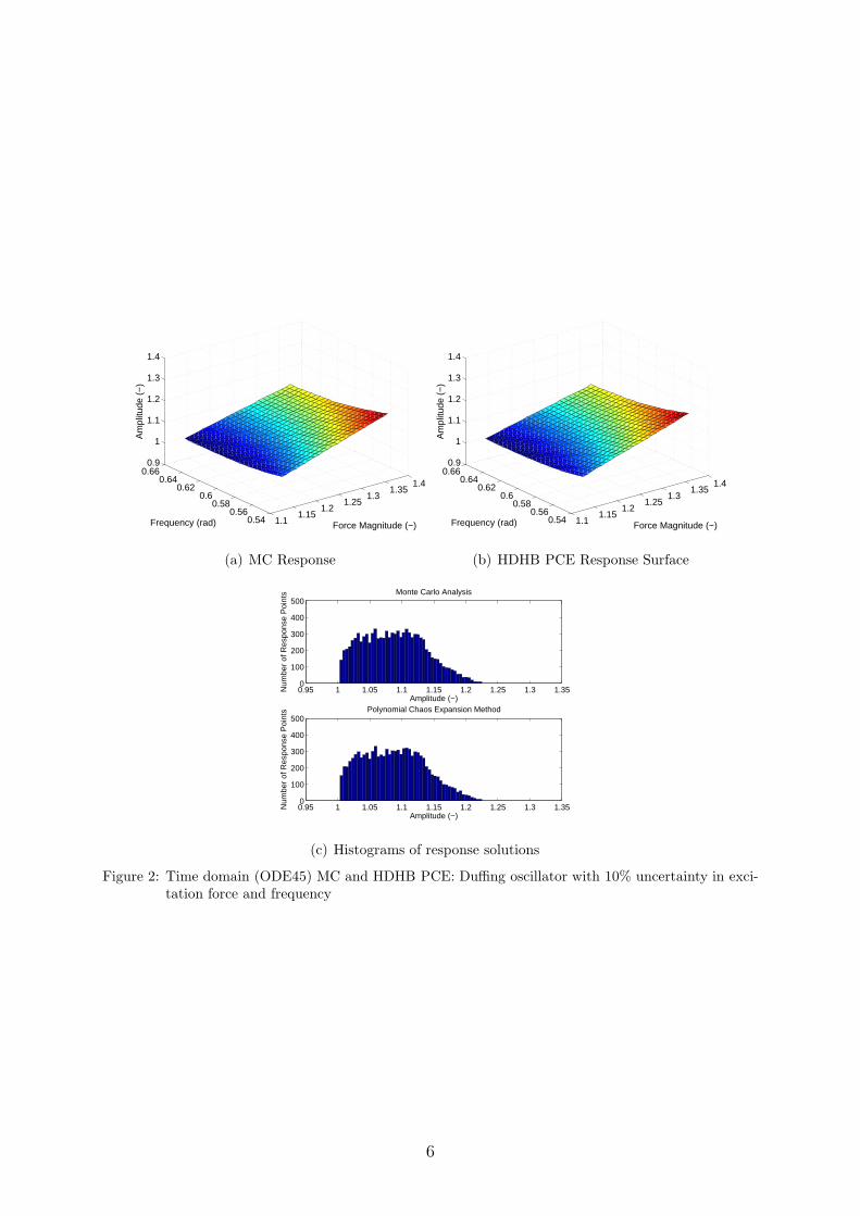
The described polynomial chaos expansion model was compared with a Monte Carloanaylsis consisting of 10000 latin hypercube sample points for both the time domain andHDHB approaches. The number of sample points used is dependent on the number of un-certain variables and the order of the interpolating polynomial function. For the Duffingoscillator a fifth order polynomial expansion was implemented where 44 latin hypercubesample points were employed with a supplementary 8 sample points at the corners andedge midpoints of the parametric space to improve robustness near the boundaries. Figure2 compares the Monte-Carlo, time integration, response with the response surface gener-ated from the HDHB polynomial chaos expansion (PCE). It is clear that the PCE methodhas successfully replicated the behaviour of the system displayed by the MC simulations.It can be seen that amplitude of the response is affected by both the magnitude andfrequency of the applied force in an almost linear manner at these conditions, despite thehighly nonlinear properties of the motion itself. The histograms in Figure 2(c) show thefrequencies of the amplitude values over the response surface and highlight the excellentagreement between the MC and HDHB-PCE methods.

The results for the HDHB PCE method shown in Figure 2 and are almost identical tothat of the time marching solutions. It was found that the ±10% variation in excitation

5

1.11.15

1.21.25

1.31.35

1.4

0.540.56

0.580.6

0.620.64

0.660.9

1

1.1

1.2

1.3

1.4

Force Magnitude (−)Frequency (rad)

Am

plitu

de (

−)

(a) MC Response

1.11.15

1.21.25

1.31.35

1.4

0.540.56

0.580.6

0.620.64

0.660.9

1

1.1

1.2

1.3

1.4

Force Magnitude (−)Frequency (rad)

Am

plitu

de (

−)

(b) HDHB PCE Response Surface

0.95 1 1.05 1.1 1.15 1.2 1.25 1.3 1.350

100

200

300

400

500

Amplitude (−)

Num

ber

of R

espo

nse

Poi

nts Monte Carlo Analysis

0.95 1 1.05 1.1 1.15 1.2 1.25 1.3 1.350

100

200

300

400

500

Amplitude (−)

Num

ber

of R

espo

nse

Poi

nts Polynomial Chaos Expansion Method

(c) Histograms of response solutions

Figure 2: Time domain (ODE45) MC and HDHB PCE: Duffing oscillator with 10% uncertainty in exci-tation force and frequency

6

Table 1: Duffing oscillator: Amplitude properties

Amplitude property Time marching HDHB methodMC mean 1.088173 1.088094PCE mean 1.088032 1.088066MC std deviation 4.701390× 10−2 4.804260× 10−2

PCE std deviation 4.703094× 10−2 4.799290× 10−2

Table 2: Duffing oscillator: Computational times

Time (s)Method MC PCETime marching 9984 272HDHB, NR 115 4HDHB, Euler 1880 48HDHB, RK4 7075 181

magnitude and frequency gives an amplitude response range of 1.0885+13.5%−7.2% . Table 1

shows the mean and standard deviation of the amplitude of the motion found by thedifferent methods. It is clear that in this case all methods used here provide very similarresults, note that the standard deviation is slightly higher for the HDHB method but thisimproves marginally with additional harmonics.

For comparison the HDHB system was also solved using an Euler pseudo-time marchingscheme and a fourth order Runge-Kutta (RK4) scheme where the results were identicalto the Newton-Raphson (NR) method so they are not shown here. The computationaltime associated with each method is displayed in Table 2 which clearly demonstratesthe potential associated with HDHB and PCE alike. By implementing PCE in a HDHBsystem solved by a Newton-Raphson scheme time savings of over 99.95% can be achievedrelative to time marching Monte carlo analysis.

4.2 Pitch-Plunge Aerofoil

In this section a typical aerofoil section restricted to pitch and plunging motions is anal-ysed. The test case used is described in detail by Lee et al. [19]. The equations of motioncan be written as:

ξ + xαα+ 2ζξω

U∗ξ +

(

ω

U∗

)2

kξξ = −1

πµCL(τ) + P (τ)

b

mU2(14)

xα

r2αξ + α + 2ζα

1

U∗α +

(

1

U∗

)2

(kαα + βαα3) =

2

πµr2αCM(τ) +

Q(τ)

mU2r2α(15)

where ξ is the non-dimensional plunge displacement of the elastic axis and α is pitch.After the introduction of four new variables, w1, w2, w3, w4 the equations of motion canbe written as:

c0ξ′′ + c1α

′′ + c2ξ′ + c3α

′ + c4ξ + c5ξ3 + c6α + c7w1 + c8w2 + c9w3 + c10w4 = f(τ) (16)

d0ξ′′ + d1α

′′ + d2α′ + d3α+ d4α

3 + d5ξ′ + d6ξ + d7w1 + d8w2 + d9w3 + d10w4 = g(τ) (17)

f(τ) and g(τ) represent part of the generalized aerodynamic forces and damp out withtime hence are not part of the periodic solution. The nonlinearity is considered only in

7

the pitch degree of freedom therefore c5 = 0. Expressions for the other coefficents aregiven in [19]. Implementing the HDHB approach to (16-17) a system in the frequencydomain can be created.

(c0ω2A2 + c2ωA+ c4I)Qξ + (c1ω

2A2 + c3ωA+ c6I)Qα + c7Qw1. . .

+c8Qw2+ c9Qw3

+ c10Qw4= 0

(d0ω2A2 + d5ωA+ d6I)Qξ + (d1ω

2A2 + d2ωA+ d3I)Qα + d7Qw1. . .

+d8Qw2+ d9Qw3

+ d10Qw4+ d4Mα = 0

(ωA+ ǫ1I)Qw1− Qα = 0

(ωA+ ǫ2I)Qw2− Qα = 0

(ωA+ ǫ1I)Qw3− Qξ = 0

(ωA+ ǫ2I)Qw4− Qξ = 0

(18)

as shown by Liu et al. [14], the system can be simplified to:

(A2 −B2B1−1A1)Qα + d4E(E

−1Qα)3= 0 = R(ω, αi), i = 0, 2, 3, ..., 2NH (19)

Unlike the Duffing oscillator the frequency of the response of the aerofoil is not constrainedby an external excitation, hence it must be treated as a variable in conjunction with theamplitude properties in order to capture the true behaviour of the system. This is achievedby letting α1 = 0 which will affect only the phase of the solution thus creating a systemof 2NH + 1 equations with 2NH unknowns. The frequency can then be simultaneouslysolved along with the Fourier coefficients using a Newton-Raphson scheme given by:

Sn+1 = Sn− λJ−1Rn (20)

where Sn is the solution vector at iteration n, λ is a relaxation parameter for increasedstability, J−1 is the inverse Jacobian of the system and Rn is the residual of (19) at iter-ation n. The solution and residual vectors are given by:

Sn =

ω

α0

α2...

α2NH

n

and Rn =

R0

R1

R2...

R2NH

n

4.2.1 Limit Cycle Oscillation Uncertainty Quantification

The system parameters used in this section are ω = 0.2, µ = 100, ah = 0.5, xα = 0.25,rα = 0.5 and ζα = ζξ = 0. A ±10% variation using a uniform distribution was imposed onthe linear and cubic stiffness coefficient with mean values of 1.0 and 3.0 respectively. Thesystem undergoes a supercritical Hopf-bifurcation as a function of the linear stiffness. Asthe bifurcation is a non-smooth function, it is difficult to be accurately represented by apolynomial function so a higher order polynomial is required by the PCE model. Howeverwith polynomials of increasing order stability and convergence degrades as shown in Figure3, requiring a higher number of samples.

To increase the performance of the polynomial interpolation more sample points wereadded including extra samples at the variable boundaries which is shown in Figure 3. It

8

0.9

0.95

1

1.05

1.1

1.15

2.6

2.8

3

3.2

3.4

0

1

2

3

4

5

6

Linear Stiffness coeff (−)Cubic Stiffness coeff. (−)

Pitc

h A

mpl

itude

(de

g)

(a) MC response

0.9

0.95

1

1.05

1.1

1.15

2.6

2.8

3

3.2

3.4

−2

0

2

4

6

Linear Stiffness coeff (−)Cubic Stiffness coeff. (−)

Pitc

h A

mpl

itude

(de

g)

(b) PCE O = 2, 28 samples

0.9

0.95

1

1.05

1.1

1.15

2.7

2.8

2.9

3

3.1

3.2

3.3

3.4

−1

0

1

2

3

4

5

6

7

Linear Stiffness coeff (−)Cubic Stiffness coeff. (−)

Pitc

h A

mpl

itude

(de

g)

(c) PCE O = 5, 52 samples

0.9

0.95

1

1.05

1.1

1.15

2.72.8

2.93

3.13.2

3.33.4

−1

0

1

2

3

4

5

6

7

Linear Stiffness coeff (−)Cubic Stiffness coeff. (−)

Pitc

h A

mpl

itude

(de

g)

(d) PCE O = 7, 80 samples (employedmodel)

Figure 3: Effect of PCE order, O on response surface generation

9

Table 3: Aerofoil: Computational times

Time (s)Method MC PCETime marching 1989 126HDHB, NR 136 9

was found that a 5th-7th order polynomial provides a reasonable approximation of theresponse surface. A much more efficient adaptive procedure was proposed in reference [11]and will be considered in the future.

The HDHB method employed just one harmonic in this as the LCO behaviour is purelysinusoidal in the absence of external forces. The statistical properties of the responses forpitch and frequency are shown in Figure 4. Both pitch and frequency variability are wellcaptured by the PCE approximation. After the bifurcation point the frequency appearsto decrease linearly (or close to it) however below the linear flutter speed the frequencyincreases rapidly as the amplitude of oscillation approaches zero. The frequency variationshows an almost constant standard deviation as U∗ increases. On the other hand, thevariability of the pitch amplitude is much more nonlinear, it starts by increasing but asit above U∗ ≈ 6.5 it becomes less sensitive to the uncertain parameters. As indicatedby Figure 3, there is a very abrupt change in behaviour for a critical value of the linearstiffness leading to higher variability of the response in the vicinity of this point.

The computational times for the aerofoil are shown in Table 3 which again show thepotential time savings using both HDHB and PCE methods to analyse system behaviourunder uncertainty. Note that PCE method is slower than in the Duffing oscillator due tothe increased number of sample points and the use of a higher order of polynomial. Despitethis time savings of 99.5% can still be achieved whilst obtaining results of reasonableaccuracy.

5 CONCLUSIONS & OUTLOOK

The influence of uncertainties in two nonlinear dynamical systems was investigated, a onedegree of freedom Duffing oscillator with uncertainties in excitation force and frequencyand a two degree of freedom aerofoil in incompressible, inviscid flow with uncertainties inboth linear and cubic stiffness coefficents in pitch. Both systems were simulated using timemarching and high dimensinal harmonic balance (HDHB) methods where a non-intrusivepolynomial chaos method (PCE) was implemented and compared with Monte Carlo (MC)results. The HDHB method showed real potential by modelling the system at a smallfraction of the cost associated with time marching methods. The PCE method provedextremely effective for smooth response surfaces exhibited by the Duffing oscillator andshowed significant reductions in cost in comparison with the Monte Carlo analyses. Thelimitations of PCE were highlighted when the non-smooth behaviour of the aerofoil wasexamined when reproducing the bifurcation feature proved difficult and stability issuesoccurred at the variable boundaries. It was demonstrated that by using PCE on a HDHBmodel time savings of over 99.5% with respect to a time marching MC analysis can beachieved while maintaining reasonable accuracy.

10

6.2 6.3 6.4 6.5 6.6 6.7 6.8 6.9 70

2

4

6

8

10

12

14

16

18

U*

α [°

]

DeterministicPCE − Mean ± 2σMC − Mean

(a) Pitch Amplitude Variation

6.2 6.3 6.4 6.5 6.6 6.7 6.8 6.9 70.078

0.079

0.08

0.081

0.082

0.083

0.084

0.085

0.086

0.087

0.088

U*

ω [r

ad/s

]

Deterministic

PCE − Mean ± 2σ

MC − Mean

(b) Frequency Variation

13.5 14 14.5 15 15.5 16 16.5 17 17.5 180

100

200

300

400

500

600

Pitch Amplitude (deg)

Num

ber

of R

espo

nse

Poi

nts

Monte Carlo Analysis

13.5 14 14.5 15 15.5 16 16.5 17 17.5 180

100

200

300

400

500

600

Pitch Amplitude (deg)

Num

ber

of R

espo

nse

Poi

nts

Polynomial Chaos Expansion Method

(c) Pitch Amplitude Histogram - U∗ = 6.9

0.078 0.079 0.08 0.081 0.082 0.083 0.084 0.085 0.0860

50

100

150

200

250

300

350

Frequency (rad/s)

Num

ber

of R

espo

nse

Poi

nts

Monte Carlo Analysis

0.078 0.079 0.08 0.081 0.082 0.083 0.084 0.085 0.0860

50

100

150

200

250

300

350

Frequency (rad/s)

Num

ber

of R

espo

nse

Poi

nts

Polynomial Chaos Expansion Method

(d) Frequency Histogram - U∗ = 6.9

Figure 4: Aerofoil Response subject to 10% variations in linear and cubic stiffness coefficents

11

6 REFERENCES

[1] Noll, T. E., Brown, J. M., Perez-Davis, M. E., et al. (2004). Investigation of thehelios prototype aircraft mishap. Tech. rep., NASA.

[2] Janardhan, S. and Grandhi, R. (2004). Uncertainty quantification in aeroelasticity:Recent results and research challenges. Journal of Aircraft, 41(5), 1217–1229.

[3] Marques, S., Badcock, K., Khodaparast, H., et al. (2010). Transonic aeroelasticstability predictions under the influence of structural variability. Journal of Aircraft,47(4), 1229–1239.

[4] Marques, S., Badcock, K., Khodaparast, H., et al. (2012). How structural modelvariability influences transonic aeroelastic stability. Journal of Aircraft, 49(5), 1189–1199.

[5] Bunton, R. and Denegri, C. (2000). Limit cycle characteristics of fighter aircraft.Journal of Aircraft, 37(5), 916 – 918.

[6] Thomas, J., Dowell, E., Hall, K., et al. (2004). Modeling limit cycle oscillationbehavior of the f-16 fighter using a harmonic balance approach. Tech. rep., AIAA.Presented at the AIAA/ASME/ASCE/AHS/ASC Structures, Structural Dynamics,and Materials Conference.

[7] Badcock, K. J., Khodaparast, H., Timme, S., et al. (2011). Calculating the influenceof structural uncertainty on aeroelastic limit cycle response. AIAA paper 2011-1741, AIAA. Presented at the 52nd AIAA/ASME/ASCE/AHS/ASC Structures,Structural Dynamics, and Materials Conference.

[8] Liu, L., Dowell, E., and Thomas, J. (2007). A high dimensional harmonic balanceapproach for an aeroelastic airfoil with cubic restoring forces. Journal of Fluids andStructures, 23(3), 351 – 363. ISSN 0889-9746. doi:10.1016/j.jfluidstructs.2006.09.005.

[9] Dimitriadis, G. (2008). Continuation of higher-order harmonic balance solutionsfor nonlinear aeroelastic systems. Journal of Aircraft, 45(2), 523–537. doi:10.2514/1.30472.

[10] Beran, P. S., Pettit, C. L., and Millman, D. R. (2006). Uncertainty quantificationof limit-cycle oscillations. Journal of Computational Physics, 217(1), 217 – 247.ISSN 0021-9991. doi:10.1016/j.jcp.2006.03.038. ¡ce:title¿Uncertainty Quantificationin Simulation Science¡/ce:title¿.

[11] Meitour, J. L., Lucor, D., and Chassaing, J. (2010). Prediction of stochastic limit cy-cle oscillations using an adaptive polynomial chaos method. Journal of Aeroelasticityand Structural Dynamics, 2(1), 3–22.

[12] Witteveen, J. A., Loeven, A., Sarkar, S., et al. (2008). Probabilistic collocation forperiod-1 limit cycle oscillations. Journal of Sound and Vibration, 311(12), 421 – 439.ISSN 0022-460X. doi:10.1016/j.jsv.2007.09.017.

[13] Hall, K., Thomas, J., and Clark, W. (2002). Computation of unsteady nonlinear flowsin cascades using a harmonic balance technique. AIAA Journal, 40(5), 879–886.

12

[14] Liu, L., Thomas, J., Dowell, E., et al. (2006). A comparison of classical and highdimensional harmonic balance approaches for a duffing oscillator. Journal of Compu-

tational Physics, 215(1), 298 – 320. ISSN 0021-9991. doi:10.1016/j.jcp.2005.10.026.

[15] Manan, A. and Cooper, J. (2009). Design of composite wings including uncertainties:A probabilistic approach. Journal of Aircraft, 46(2), 601–607, doi: 10.2514/1.39138.

[16] Allen, M. and Camberos, J. (2009). Comparison of uncertainty propagation / re-sponse surface techniques for two aeroelastic systems. AIAA Paper 2009-2269, AIAA.Presented at the AIAA/ASME/ASCE/AHS/ASC Structures, Structural Dynamics,and Materials Conference, Palm Springs, California.

[17] Hosde, S., Walters, R., and Balch, M. (2010). Point-collocation nonintrusive poly-nomial chaos method for stochastic computational fluid dynamics. AIAA Journal,48(12), 2721–2730, doi: 10.2514/1.39389.

[18] Marques, S. and Badcock, K. (2011). Stochastic optimisation of transonic aeroelas-tic structures. IFASD 2011-17, AAAF. Presented at the International Forum forAeroelasticity and Structural Dynamics, Paris, France.

[19] Lee, B., Liu, L., and Chung, K. (2005). Airfoil motion in subsonic flow with strongcubic nonlinear restoring forces. Journal of Sound and Vibration, 281(35), 699 – 717.ISSN 0022-460X. doi:10.1016/j.jsv.2004.01.034.

13