uncertainty and climate change

Environmental and Resource Economics 22: 3–39, 2002.© 2002 Kluwer Academic Publishers. Printed in the Netherlands.

3

Uncertainty and Climate Change

GEOFFREY HEAL1 and BENGT KRISTRÖM2

1Columbia Business School, New York, NY 10027, USA (E-mail: [email protected])2SLU-Umeå, 901 83 Umeå, Sweden

Abstract. Uncertainty is pervasive in analysis of climate change. How should economists allow forthis? And how have they allowed for it? This paper reviews both of these questions.

Key words: climate change, risk, uncertainty

1. Overview

The extent to which the earth’s climate will change as a result of human activityis still unclear. Although the basic science is well-understood and now seemsconfirmed by the data available, the precise magnitudes of the various effects thatcontribute to the climate regime are not yet known. The most recent assessment bythe UN Intergovernmental Panel on Climate Change (IPCC), the Third AssessmentReport (TAR), has for the first time made an explicit attempt to give an indicationof the degrees of uncertainty associated with its various predictions.1 The TARgives an indication of the degree of confidence that the leading authorities in thefield of climate change have in their forecasts. In some cases it is clear that, whilethe sign of an impact is clearly known, there remains massive uncertainty aboutthe size, with the range of possible magnitudes involving differences of severalhundred percent. This is illustrated by the IPCC’s widely-quoted range for thepossible change in global mean temperature, which goes from 1.5 to 6 degreescentigrade.2 In the TAR the IPCC classifies its findings according to the degree ofconfidence in them. It recognizes five different confidence levels, ranging from veryhigh (≥95%) through high (67 ≤ X ≤ 95%) medium (33 ≤ X ≤ 67%) to very low(≤5%). Most of its major findings are assigned one of these probability rankings,which in general are assumed to correspond to Bayesian subjective probabilities.In cases in which a Bayesian characterization is considered inappropriate, largelybecause the state of knowledge is too primitive, the IPCC TAR uses a four-wayclassification (Table I). This classification distinguishes four cases: the most certainis a high level of agreement between scientists and a substantial amount of evidenceon the issue, but not enough to distinguish between the competing theories: theopposite case is low agreement about the alternative theories and little evidenceto distinguish between them. They characterize this as a situation where theanalysis has to be “speculative”. So while there is widespread agreement that our

4 GEOFFREY HEAL AND BENGT KRISTRÖM

Table I. IPCC TAR classifications.

Level of Amount of evidence (observations, model output, theory, etc.)

agreement Low High

High Established but incomplete Well-established

Low Speculative Competing explanations

climate is changing, there remains uncertainty about the possible magnitude of thechange.

As economists, it is not only uncertainty about the underlying climate sciencethat should be of concern to us. Ultimately we are interested in the impact ofclimate change on human societies, and this involves knowing not only how theclimate may alter but also how changes in the climate regime translate into impactsthat matter for humans. How do climate changes translate into changes in agri-cultural production, into changes in the ranges of disease vectors, into changesin patterns of tourist travel, even into feelings of well-being directly associatedwith the state of the climate? So we are concerned here about the outcome of aprocess with at least two stages: stage one is a change in the climate regime andstage two is the translation of this into changes in things that matter directly tous. Even if we knew exactly what the climate would be in 2050, we still wouldface major economic uncertainties because we currently do not know how alteredclimate states map into human welfare.

In assessing the economics of climate change there are therefore at least twosources of uncertainty – what the climate will be, and what any given changedclimate will mean in economic terms. We can think of these as the scientific uncer-tainties analyzed by the IPCC’s TAR, and the uncertainties about climate impacts.In fact there is a third stage, uncertainty about the policies that we will chooseto control emissions over the coming decades. So in trying to forecast what theclimate will be at a future date such as 2050 we have not only to forecast how theclimate system will respond to human influence but also what that influence willbe: what policies will be chosen in the interim.

In total, we seem to have to take account of scientific uncertainty, impactuncertainty and policy uncertainty. Possible policy responses to climate changetake two forms: mitigation, i.e., actions that reduce the flow of greenhouse gasesinto the atmosphere and, thereby, change the probability distribution over futureclimate states; and adaptation – actions that reduce the damages associated witha given climate state.3 Both provide sources of uncertainty. In the domain ofmitigation, perhaps the most prominent source of uncertainty is institutional: willthe international community adopt aggressive mandates to restrict emissions ofgreenhouse gases? Will the institutions that implement these mandates be efficient,i.e., will the marginal cost of net reductions in emissions be roughly equal across

UNCERTAINTY AND CLIMATE CHANGE 5

all sources and sinks? What technical changes will appear to reduce the costs ofmitigation? Adaptation likewise involves uncertainty about the different optionsthat will become available, and their costs.

The IPCC TAR goes further and recognizes no less than five stages of uncer-tainty, as a result of breaking down the scientific uncertainty into sub categories. Itsfive categories are uncertainty about emission scenarios (i.e. about anthropogenicemissions of greenhouse gases), about the responses of the carbon cycle to theseemissions, about the sensitivity of the climate to changes in the carbon cycle, aboutthe regional implications of a global climate scenario, and finally uncertainty aboutthe possible impacts on human societies. We have noted the first of these – uncer-tainty about emissions scenarios. And we aggregate the next three (concerningthe response of the carbon cycle, the sensitivity of the climate system and theregional implications of global scenarios) as these are all “scientific uncertainty”from the perspective of an economist. This leaves the final category of uncertaintyas impacts.The TAR has a diagram that shows the degree of uncertainty rising aswe move through these five stages, with the error bars growing from stage to stage.

Uncertainty can of course be reduced through learning. This consideration leadsto a second-order, or meta- form of uncertainty: what new information will berevealed to resolve the present uncertainties? To what extent can and will researchaccelerate the pace of learning? Given the possibility of future learning, issues ofirreversibility and quasi-option value may become salient.

This discussion suggests clearly that any economic analysis of climate changeshould include uncertainty as a central feature. Yet a review of the literature showsthat the bulk of the work to date has been deterministic, though there are exceptionsand the trend is changing. If uncertainty is central then attitudes towards risk andthe degree of risk aversion will presumably be central parameters. Institutions forrisk-shifting will also be important, and the possibility that some changes are irre-versible and that we may learn more about them with the passage of time suggeststhat real option values may also matter in the analysis of policy measures. Anotheranalytically interesting feature of climate change is that the risks are not exogenous,as in many models of uncertainty in economics, but are generated by our own activ-ities. This endogeneity of the risks raises questions about the use of markets andinsurance for hedging some of the risks associated with possible climate change:there is the macro-level equivalent of moral hazard here. Finally, as many authorshave remarked, the time horizon implicit in climate change is very long indeed,measured in centuries, far longer than economists are used to. Uncertainties arealmost inevitably large when decisions involve such long time horizons. In sum: inanalyzing climate change policies, attitudes towards risk will be important, as maybe the values of maintaining certain options open.

Endogeneity of risks may pose some problems for the use of certain types offinancial institutions, and the length of the time horizon will pose a challenge toour normal ideas about discounting.4 As the preceding discussion indicates, theeconomic problem of climate management cleaves (usefully, if imperfectly) into


four parts. Section 2 summarizes what climate scientists can tell us about the mainsources of uncertainty in the relationship between greenhouse gas emissions andfuture climate states. Section 3 addresses the relationship between future climatestates and impacts on human welfare. Section 4 sets out the basic economic issues,and summarizes some calculations indicative of the possible importance of keyeconomic parameters. In section 5 we set out a very general model that seems toincorporate most of the central issues. This model is too complex to be solvedanalytically, and we then review the models that have actually been solved todate, most of which can be seen as special cases of this framework. In subsequentsections we look at a range of issues relating to the management of climate risksby economic institutions such as financial markets, and the impact of uncertaintyand the endogeneity of risks on these institutions.

2. Uncertainty in the TAR

To set the stage, we begin by surveying the area where economics has the leastdirect relevance: understanding the relationship between greenhouse gas buildupand possible future climate states. What can the scientific community tell us aboutthese relationships, and with what degree of certainty? The basic physics of climatechange is well-understood and not controversial, and has been known for over acentury. Uncertainties arise when applying the physical principles via complexcomputer models with many parameters that have to be estimated or calibratedfrom inadequate data sets. These are issues to which economists can surely relate!

So most of the central numerical estimates are subject to considerable error,as indicated by the flagship prediction of the IPCC that global mean temperaturewill change by between 1.5 and 6 degrees centigrade by 2100 relative to 1990 –a difference of a factor of four between the top and bottom of the range. To befair we have to recall that this is a 100 year forecast – how many economistswould want to put their names to forecasts for 2100? Probably we would findthat the range of social and economic uncertainties is even greater if we were tothink about it. Many of the uncertainties that appear in the forecasts arise naturallyfrom the length of the time horizon considered combined with the uncertaintiesin the model parameters. Specific issues that make an additional contribution touncertainty include the impacts of aerosols – fine particles in the air often causedby pollution – on the condensation of water vapor and the formation of clouds, andmore generally the formation of clouds. Clouds reflect sunlight back into space andso control warming to some degree, and little is understood numerically about theirformation, though it is known that fine particles in the air provide nuclei on whichwater droplets can form and start the process of cloud formation.

A rather different source of uncertainty is the possible failure of the thermo-haline circulation system in the north Atlantic: this is the technical name for theGulf Stream that brings hot water from the tropical regions to northern Europe.This massive heat transfer is largely responsible for the comparatively benign


climate of northern Europe relative to those of other regions at the same latitude,and there is evidence that during past climate fluctuations this system has stopped,leading to massive cooling in Europe. Computer models do indicate that atmo-spheric warming by greenhouse gases could switch off this massive heat transfersystem, with dramatic results for the climates of many densely populated regions.5

However, the IPCC assigns a “low” probability to this. The fact that something is alow probability event does not of course mean that it does not matter economically– if the consequences are sufficiently dramatic then this may more than compensatefor the low likelihood and mean that the expected loss is still significant. So theIPCC’s comment that something is “low probability” does not mean that as socialscientists we should neglect it; this depends on the consequences.

Other issues that are still not resolved at the scientific level concern the behaviorof terrestrial carbon sinks at higher temperatures and carbon dioxide concentra-tions, and also the behavior of the oceans both as heat sinks and as carbon sinks.As the oceans sequester more carbon than the terrestrial biosphere and are a majorelement in the planet’s heat transfer system, this lack of detailed understandingtranslates into a significant source of uncertainty.

3. Climate Change and Human Welfare

Changes in climate have effects on human welfare through many pathways. Todate most studies have considered the impact of climate change on agriculturalproductivity and on sea level and indeed have more or less equated the overallimpact of climate change with these impacts. We are beginning to see that thisis probably a very restricted and limited view of climate change and its humanimpacts. There are suggestions emerging that climate has an impact on economicdevelopment and on the pattern of economic growth. There are also suggestionsthat climate affects human welfare directly, not via agricultural output or economicdevelopment but as an argument of the utility function. Climate changes will alsoaffect the occurrence of extreme events and the geographical range of many diseasevectors such as the malarial pathogens.

David Landes (1998) includes climate as one of the key factors in his widelyread (and controversial) “The Wealth and Poverty of Nations”. Tropical diseases,access to water, the propensity to natural disasters, etc. present regions like Africawith a handicap, according to Landes. He also presents an account of geographersand others who marshalled climate as the key variable to explain economic differ-ences. In a similar vein is a recent study by Horowitz (2001). He carried out aregression that addresses the relationship across countries between average annualtemperature and GDP per head, looking at the income-temperature relationshipfor a cross-section of 156 countries in 1999. As is well known, hotter countriesare poorer on average. The widespread belief is that this relationship is mostlyhistorical; that is, due to a past effect of climate. Acemoglu, Johnson, and Robinson(2001) have recently made great gains in identifying a specific historical path for


this relationship. They posit that mortality rates of early colonizing settlers had aprofound effect on the institutions that were set up in those colonies. These institu-tional differences persist to this day, they argue, and have strong effects on currentincomes. Because colonial mortality and average temperature are highly correlated,the mortality-income relationship also manifests itself as an income-temperaturerelationship. Horowitz argues that there is, however, sufficient evidence to warrantcontinued examination of the income-temperature relationship. He finds a strongincome-temperature relationship within OECD countries, a result that does notappear to be predicted by the colonial mortality model. He also finds that theincome-temperature relationship is essentially the same within the OECD and non-OECD countries, a striking yet unremarked and as-yet unexplained result. Finallyhe finds a strong income-temperature relationship within the fifteen countries of theformer Soviet Union, where colonial institutions would seem to have been wipedout. His best measure of the effect of temperature on income, after accountingfor the influence of colonial mortality, is that a one percent increase in temperatureleads to a −0.9 percent decrease in per capita income. Thus, a temperature increaseof 3 degrees Fahrenheit would result in a 4.6 percent decrease in world GNP. Theresult is striking. While the result is only suggestive – there is no causal mechanismoffered – it suggests that there is a relationship between temperature and economicproduction, and that changes in temperature may, then, create first-order changesin economic output and welfare.

Similar conclusions are emerging from other related studies. Gallup, Sachsand Mellinger (1998) have suggested that tropical climates make economic devel-opment more difficult, via reduced agricultural productivity and added diseaseburden. They do not specifically comment on the economic consequences ofclimate change but an implication of their findings is surely that as “tropical”climates become more widespread then so will their economic disadvantages.Similar conclusions are suggested by Gavin and Hausman (1998). All of the resultsthat tie climate to economic development are tentative and are too preliminaryto form the basis for quantitative estimates of welfare impacts. They represent amechanism through which climate change can have economic consequences whichhas been little explored to date, and consequently is a source of uncertainty in anyestimates of climate change impacts.

3.1. DIRECT EFFECTS ON HUMAN WELL-BEING

There is a clear connection between weather, climate, and how well people feel.We dislike very cold climates and very hot ones, and possibly also very humidones. There are probably good reasons for these likes and dislikes, founded inevolutionary biology. In this context, Maddison and Bigano (2000) find that themost popular tourist destinations are those offering temperatures of around 88 ◦F(31 ◦C): this appears to be an “ideal temperature”, at least for the inhabitants ofwestern Europe. Lise and Tol (2001) find similar results. They carry out a cross-


section analysis on destinations of OECD tourists and a factor and regressionanalysis on holiday activities of Dutch tourists, to find optimal temperatures attravel destination for different tourists and different tourist activities. Globally,OECD tourists prefer a temperature of 21 ◦C (= 70 ◦F) (average of the hottest monthof the year) at their choice of holiday destination. This finding and Maddison’sresults indicate that, under a scenario of gradual warming, tourists would spendtheir holidays in different places than they currently do. It also suggests that astemperatures change as a result of global warming there could be a loss of welfarein some regions just because of the climate change itself and quite independentlyof any consequences for economic activity.

It seems a very safe assumption that human preferences about temperature arebiologically determined and are likely, therefore, to be stable over time. This isnot to deny that temperature preferences may well exhibit cross-sectional variationacross cultures and ethnic groups. Insofar as people are biologically or culturallyadapted to particular climes, change may be bad per se. In some sense this is just anextension of the argument that plants and animals that are adapted to certain climateconditions will suffer from climate change. Humans are just one of many speciesof animals, albeit an unusually disruptive one, and so in principle are subject to thesame effects. The direct effects of climate on human welfare are probably the leastexplored of all effects so far, and could be some of the more important, especiallyfor populations in areas where agriculture will not be greatly affected by a changedclimate regime. They are therefore a major source of uncertainty.

4. The Economic Framework

That discount rates and attitudes to the far future matter in assessing climate changehas always been clear. Now it should also be clear that risk aversion will matter aswell. An important implication of this is that even though an event is very unlikely,if it is costly and we are risk averse we may invest significantly in avoiding it orinsuring against it. By way of illustration, our houses rarely burn down, yet mostof us insure them against this event on terms that are actuarially unfair.

In the context of climate change there is a real potential for learning overtime. Global circulation models have been greatly refined and enhanced since theirfirst use in analyzing climate change, and this has improved our understanding ofwhat might happen. There are many other ways in which our understanding mightimprove in the future. We might learn about cleaner energy production technolo-gies, or about novel methods of carbon sequestration. Over several decades thechanges in our understanding of these possibilities could be far-reaching. Signifi-cant changes in our understanding of these possibilities could alter the relativemerits of different economic policies. As an illustration, Lackner et al. (1999) haveproposed the sequestration of carbon dioxide by using calcium hydroxide, andthe scrubbing of emission gases from fossil fuel plants using the same chemical(spraying tropical waters with iron filings is another geoengineering suggestion,


see Keith (2000) for a review). The possibility of implementing this on a large scaleis still speculative and will remain so for some years, but this discussion offers atantalizing glimpse of the kind of qualitative technological change that might occurwithin the next few decades.

4.1. IRREVERSIBILITY

It is also likely that many of the changes in climate, and changes in the naturalenvironment driven by climate change, will be irreversible. The consequences ofthis possible irreversibility have been discussed at great length, if rather incon-clusively, so it is important to understand the underlying issues. Changes in theclimate may in themselves be irreversible: once the climate regime in an area haschanged, it may not be possible to restore the original. The most notable case ofthis arises from the possible change in the path of the Gulf Stream, a possibility thatwe mentioned as one of the biggest sources of uncertainty in forecasting climateregimes. The issue here is that the climate system is a complex nonlinear dynam-ical system and like most such systems has several possible equilibrium states orattractors. Each has a basin of attraction – a set of initial conditions within whichit is stable, in the sense that if the initial conditions are within the basin then thesystem moves to that equilibrium. Stresses on the system, such as human changesto the mix of gases in the atmosphere, could possibly move the climate systemfrom one basin of attraction to another. Moving from one configuration of the GulfStream to another would be an example of this. Once the system is in a new basinof attraction it is not obvious that we could move it back to the original, so such achange may be irreversible.

Possible irreversibilities may also arise because the climate is determined byinteractions between the atmosphere, the oceans and the biosphere. Changes inthe climate might lead to changes in oceans or the biosphere that would make therestoration of the original configuration impossible. For example, the climate of theAmazonian region is created in part by the forests there; trees in the forest transpirevast quantities of moisture into the air and contribute to the humidity of the region.Were the region to become hotter and drier, these trees would die and consequentlythe soils would change. Reducing the concentration of greenhouse gases in theatmosphere would then probably not restore the original climate to the Amazonianregion because the forest would have died and could not be restarted, and was akey element of the original climate system. Another irreversible aspect of climatechange would be the melting of the west antarctic ice sheet, which would lead to asignificant and rapid increase in sea levels globally.

Issues of how far climate changes could be reversed by reducing greenhousegas concentrations have not been extensively studied, although in most economicmodels they are modelled as if the changes in climate can eventually be reversed,even if slowly. Even if changes in the climate were to be reversible, there are otherassociated changes that might not be. For example, climate changes might drive


certain species extinct if their habitats are destroyed: indeed increased extinctionrates are a widely-forecast consequence of climate change. Extinction is self-evidently not a reversible process. At a more mundane level, climate changewill alter plant and animal communities in ways that may make it impossibleto reestablish the original community even if the components are not extinct. Inthis vein, an expected consequence of climate change is the death of some coralreefs. This will lead to changes in marine communities that will not be reversibleon human timescales. This combination of potential for learning together withirreversibilities is the classical breeding ground for real option values. If climatechange or its consequences are indeed irreversible and there is a chance of learningmore over time, then there may be a real option value associated with preserving thepresent climate regime, i.e. with freezing all actions that are likely to contribute toclimate change. This real option value could reinforce the widely-cited but seldomanalyzed “precautionary principle,” a nostrum to the effect that we should avoidmaking possible environmental changes until we are sure of their consequences.However, confusingly, there is another possible real option value at work here.Suppose that substantial sunk costs must be incurred to begin the process of abatinggreenhouse gas emission and avoiding or minimizing climate change. The return tothis investment is the avoidance of climate change and if we learn about the valueof this over time then there is also a real option value associated with postponinginvestment in greenhouse gas abatement. So there could also be an “inverse precau-tionary principle” at work here suggesting that we avoid costly policies requiringirreversible investments until we are really sure that they are needed.

Striking a balance here is made more complex by the fact that it is not onlythe time horizons that are long, but also the time lags in many parts of the system.Both climate and economic systems are likely to respond very slowly to policiesimplemented to change greenhouse gas emissions. So even if a forceful greenhousegas abatement policy were implemented tomorrow, its impact might not be felt onemission levels until 2010 or later, and the consequences for the climate of a reduc-tion in GHG flows beginning in 2010 or later would be slight prior to 2020 at thevery earliest. There would be further lags between changes in climate trends and thetrends in the factors that affect humans – agriculture, diseases, etc. Consequentlythere is an argument that as there is a real risk that the climate will be seriouslyperturbed by human action by say 2040, and as the lags in the systems that linkour policies to the outcomes that matter are so long, then we have a responsibilityto start taking actions now, as actions taken later will be too late to avoid harm tothose living in 2040.

By now it is clear that setting out a convincing analytical framework for climatepolicy choices is a challenge: the intrinsic uncertainties enter in many differentways. Next we take a look at how these issues could in principle be captured, andhow they have actually been captured, in the literature to date.


4.2. PRELIMINARY CALCULATIONS: THE VALUE OF AVOIDING CLIMATE

CHANGE

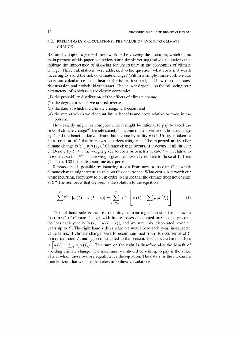
Before developing a general framework and reviewing the literature, which is themain purpose of this paper, we review some simple yet suggestive calculations thatindicate the importance of allowing for uncertainty in the economics of climatechange. These calculations were addressed to the question: what costs is it worthincurring to avoid the risk of climate change? Within a simple framework we cancarry out calculations that illustrate the issues involved, and how discount rates,risk aversion and probabilities interact. The answer depends on the following fourparameters, of which two are clearly economic:

(1) the probability distribution of the effects of climate change,(2) the degree to which we are risk averse,(3) the date at which the climate change will occur, and(4) the rate at which we discount future benefits and costs relative to those in the

present.How exactly might we compute what it might be rational to pay to avoid the

risks of climate change?6 Denote society’s income in the absence of climate changeby I and the benefits derived from this income by utility u (I ). Utility is taken tobe a function of I that increases at a decreasing rate. The expected utility afterclimate change is

∑j pju

(Ij

).7 Climate change occurs, if it occurs at all, in year

C. Denote by δ ≤ 1 the weight given to costs or benefits at date t + 1 relative tothose at t , so that δt−1 is the weight given to those at t relative to those at 1. Then(1 − δ) × 100 is the discount rate as a percent.

Suppose that it possible by incurring a cost from now to the date C at whichclimate change might occur, to rule out this occurrence. What cost x is it worth ourwhile incurring, from now to C, in order to ensure that the climate does not changeat C? The number x that we seek is the solution to the equation

C∑t=1

δt−1 [u (I ) − u (I − x)] =T∑

t=C+1

δt−1

u (I ) −

∑j

pju(Ij

) (1)

The left hand side is the loss of utility in incurring the cost x from now tothe time C of climate change, with future losses discounted back to the present:the loss each year is [u (I ) − u (I − x)], and we sum this, discounted, over allyears up to C. The right hand side is what we would lose each year, in expectedvalue terms, if climate change were to occur, summed from its occurrence at C

to a distant date T , and again discounted to the present. The expected annual loss

is[u (I ) − ∑

j pju(Ij

)]. This sum on the right is therefore also the benefit of

avoiding climate change. The maximum we should be willing to pay is the valueof x at which these two are equal: hence the equation. The date T is the maximumtime horizon that we consider relevant to these calculations.


As a concrete illustration, we can think of x as the extra cost of moving asfast as possible to energy based on non-fossil sources, such as solar, geothermalor biomass. As these technologies develop, this cost will decline: we assumethat it is zero by the time at which climate change would occur, which in theillustrative calculations is taken to be fifty years hence. Obviously there aresome heroic assumptions here. Climate change is taken to be a discrete event.Preventive expenditures are assumed to be constant. But nevertheless the numbersare interesting.

4.2.1. Results

Below we present values of x for some illustrative parameter values and indicatetheir sensitivity to the assumptions. What we should be willing to pay, x, isexpressed as a percent of the income level8 I , which is taken to be 10. The calcula-tions are only illustrative: we do not know enough about the costs or probabilitiesof climate change to make presenting a best estimate of x a useful exercise. The keyconclusion is that for some parameter values that must be within the set consideredpossible, one might wish to spend up to 8.13% of national income on avoidingclimate change. For other parameter values that are also possible, the number maybe 0.1%. Even this is a big number in absolute terms. The most critical parameterin these calculations is an economic parameter, the discount rate, which rarelyfeatures in policy discussions. The index of risk aversion is also very influential.

A reasonable functional form for the utility functions u (I ), widely usedin empirical studies of behavior under uncertainty, is the family of functionsdisplaying constant relative risk aversion: the index of relative risk aversion (IRRA)for u (I ) at income I is −Iu′′/u′ where u′ and u′′ are the first and second derivativesof u respectively. This is a measure of willingness to pay to avoid risk. Functionsfor which this index is constant are of the form I a for a > 0, −I a for a < 0,and log(I ). A reasonable range of empirical values for the index of relative riskaversion is from 2 to 6.

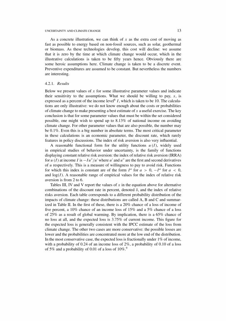
Tables III, IV and V report the values of x in the equation above for alternativecombinations of the discount rate in percent, denoted δ, and the index of relativerisks aversion. Each table corresponds to a different probability distribution of theimpacts of climate change: these distributions are called A, B and C and summar-ized in Table II. In the first of these, there is a 20% chance of a loss of income offive percent, a 10% chance of an income loss of 15% and a 5% chance of a lossof 25% as a result of global warming. By implication, there is a 65% chance ofno loss at all, and the expected loss is 3.75% of current income. This figure forthe expected loss is generally consistent with the IPCC estimate of the loss fromclimate change. The other two cases are more conservative: the possible losses arelower and the probabilities are concentrated more at the low end of the distribution.In the most conservative case, the expected loss is fractionally under 1% of income,with a probability of 0.24 of an income loss of 2%, a probability of 0.10 of a lossof 5% and a probability of 0.01 of a loss of 10%.9


Table II. Alternative probability distributions.

Probability

Loss A B C

2% 0.24

5% 0.2 0.24 0.1

10% 0.01

15% 0.1 0.10

20% 0.01

25% 0.05

0 0.65 0.65 0.65

E. loss 3.75% 2.99% 0.99%

Table III. Willingness-to-pay for distribution A.

IRRA 0 1 2 3 4 5 6

δ

1 5.74 6.07 6.42 6.81 7.22 7.66 8.13

2 2.15 2.32 2.50 2.72 2.96 3.23 3.54

3 1.05 1.13 1.23 1.35 1.48 1.64 1.82

4 0.56 0.61 0.66 0.73 0.81 0.89 1.00

5 0.31 0.34 0.37 0.41 0.45 0.50 0.56

As mentioned, the date for climate change C is assumed to be fifty years, andwe take the upper limit of the sum of benefits T to be 1000.

The tables III, IV and V report the results of solving the equation for x for theseprobability distributions and a range values for the discount rate (from 1% to 5%)and for the IRRA (from 0 to 6).

Can we pin down more precisely the most appropriate parameter ranges? Thequestion of risk aversion has not been studied in the context of climate change.However there are many empirical studies of risk aversion in finance, and therange of values for the IRRA considered to be appropriate there runs from 2 to6. The issue of the right discount rate is a controversial one: one of the foundersof dynamics economics, Frank Ramsey (1928) declared in a paper that is still inmany ways definitive that “discounting of future utilities is unethical, and arisespurely from a weakness of the imagination.”10 This implies a discount rate of zero,which in turn implies a willingness to spend from 15% to 30% of income to preventglobal warming. Most contemporary commentators have implicitly disagreed withRamsey, in many cases without clearly stating their reasons, and for the very longtime horizons involved in climate change have worked with discount rates of 1%


Table IV. Willingness-to-pay for distribution B.

IRRA 0 1 2 3 4 5 6

δ

1 4.44 4.61 4.78 4.96 5.15 5.35 5.56

2 1.66 1.75 1.84 1.95 2.06 2.18 2.31

3 0.81 0.86 0.91 0.96 1.02 1.09 1.16

4 0.43 0.46 0.49 0.51 0.55 0.59 0.63

5 0.24 0.26 0.27 0.29 0.31 0.33 0.36

Table V. Willingness-to-pay for distribution C.

IRRA 0 1 2 3 4 5 6

δ

1 1.65 1.68 1.70 1.72 1.74 1.77 1.79

2 0.62 0.63 0.64 0.65 0.67 0.68 0.69

3 0.30 0.30 0.31 0.32 0.33 0.33 0.34

4 0.16 0.16 0.17 0.17 0.18 0.18 0.18

5 0.09 0.09 0.09 0.10 0.10 0.10 0.10

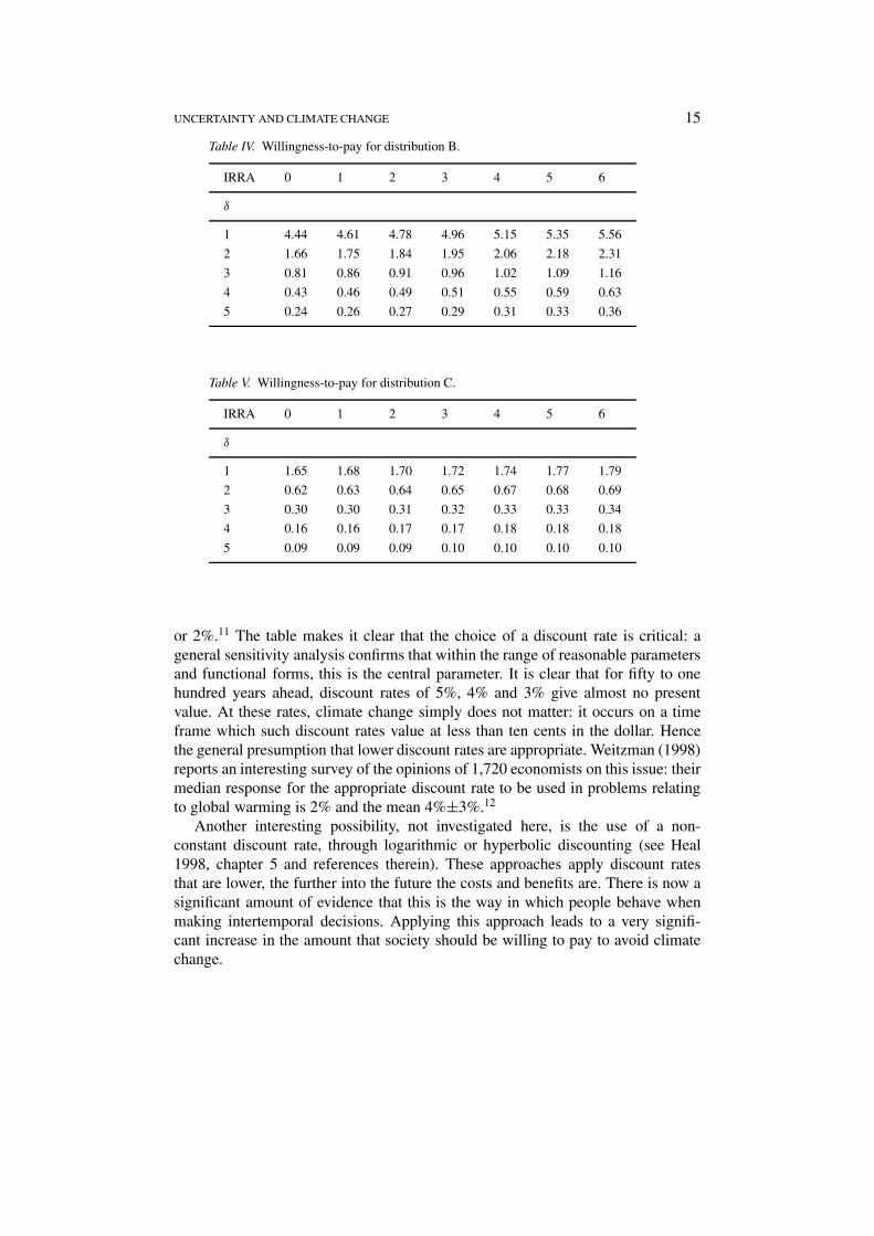
or 2%.11 The table makes it clear that the choice of a discount rate is critical: ageneral sensitivity analysis confirms that within the range of reasonable parametersand functional forms, this is the central parameter. It is clear that for fifty to onehundred years ahead, discount rates of 5%, 4% and 3% give almost no presentvalue. At these rates, climate change simply does not matter: it occurs on a timeframe which such discount rates value at less than ten cents in the dollar. Hencethe general presumption that lower discount rates are appropriate. Weitzman (1998)reports an interesting survey of the opinions of 1,720 economists on this issue: theirmedian response for the appropriate discount rate to be used in problems relatingto global warming is 2% and the mean 4%±3%.12

Another interesting possibility, not investigated here, is the use of a non-constant discount rate, through logarithmic or hyperbolic discounting (see Heal1998, chapter 5 and references therein). These approaches apply discount ratesthat are lower, the further into the future the costs and benefits are. There is now asignificant amount of evidence that this is the way in which people behave whenmaking intertemporal decisions. Applying this approach leads to a very signifi-cant increase in the amount that society should be willing to pay to avoid climatechange.


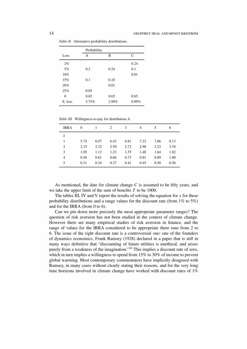
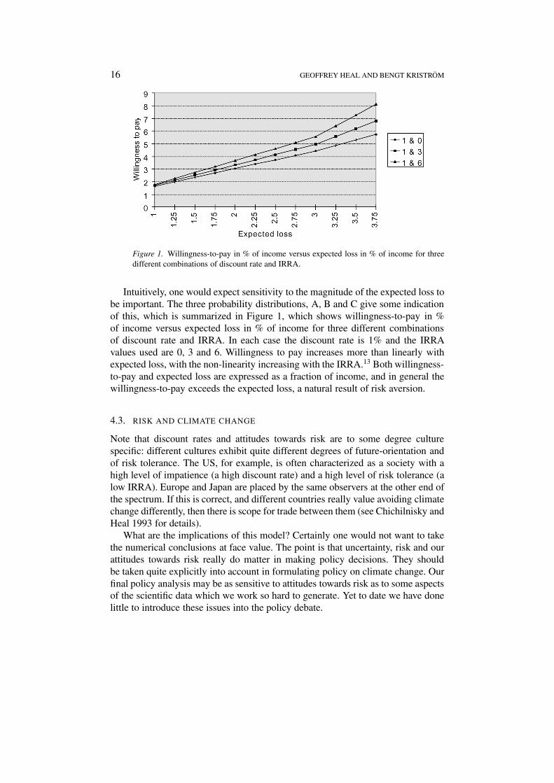
Figure 1. Willingness-to-pay in % of income versus expected loss in % of income for threedifferent combinations of discount rate and IRRA.

Intuitively, one would expect sensitivity to the magnitude of the expected loss tobe important. The three probability distributions, A, B and C give some indicationof this, which is summarized in Figure 1, which shows willingness-to-pay in %of income versus expected loss in % of income for three different combinationsof discount rate and IRRA. In each case the discount rate is 1% and the IRRAvalues used are 0, 3 and 6. Willingness to pay increases more than linearly withexpected loss, with the non-linearity increasing with the IRRA.13 Both willingness-to-pay and expected loss are expressed as a fraction of income, and in general thewillingness-to-pay exceeds the expected loss, a natural result of risk aversion.

4.3. RISK AND CLIMATE CHANGE

Note that discount rates and attitudes towards risk are to some degree culturespecific: different cultures exhibit quite different degrees of future-orientation andof risk tolerance. The US, for example, is often characterized as a society with ahigh level of impatience (a high discount rate) and a high level of risk tolerance (alow IRRA). Europe and Japan are placed by the same observers at the other end ofthe spectrum. If this is correct, and different countries really value avoiding climatechange differently, then there is scope for trade between them (see Chichilnisky andHeal 1993 for details).

What are the implications of this model? Certainly one would not want to takethe numerical conclusions at face value. The point is that uncertainty, risk and ourattitudes towards risk really do matter in making policy decisions. They shouldbe taken quite explicitly into account in formulating policy on climate change. Ourfinal policy analysis may be as sensitive to attitudes towards risk as to some aspectsof the scientific data which we work so hard to generate. Yet to date we have donelittle to introduce these issues into the policy debate.


In fact the role of risk and uncertainty in an analysis of policy towards climatechange goes much further. There are several dimensions of this role that meritparticular comment: these are the endogeneity of the risks that we face, and thefact that the risks are substantially unknown. Endogeneity of the risks is clear fromthe fact that they are anthropogenic: we create them as a result of our social andeconomic activity. It is human activity that drives biodiversity loss, climate changeand ozone depletion. That the associated risks are substantially unknown is alsoclear from the brief discussions above. Another difficult characteristic of climaterisks is that a large number of people face the same risks – the risks are correlatedacross large communities. This means that standard insurance models, relying asthey do on independent risks, are probably not appropriate as mechanisms formanaging the risks. It also means that we cannot argue, as for many risks (followingArrow and Lind 1970), that at the social level risks can be neglected as they affectindividuals and are independent and so in the aggregate cancel out.

5. A General Model

Clearly we have to work with a stochastic dynamic model in which the chance ofclimate change is affected by, and affects, economic activity and welfare. The mostnatural and widely-used model seems to be an extension of the standard optimalgrowth model along the following lines. Output is produced from capital stocksand other inputs, primarily labor. The capital stocks should include both phys-ical capital and natural capital, as some of the most important possible impactsof climate change are on the productivity of natural capital, for example on theproductivity of land or of fisheries or the value that can be generated from skiresorts. Climate change could affect land values by changing rainfall patterns,changing access to river flow, or changing the range of agricultural pathogens.

The output can as usual be consumed or invested: production also leads to aflow of greenhouse gases that cumulate into a stock. The size of this stock drivesthe probability of climate change, and so can affect output. The state of the climatecan also affect welfare directly, as we may derive well-being from the climate – wemay prefer mild dry climates to hot wet ones, for example. And it can affect humanhealth via factors like the range of disease vectors. There is evidence that the rangeof malaria has increased in parts of the world in response to changes in climate andduring El Nino events the ranges of diseases such as Dengue fever appear to varyin response to changed climate conditions.

Mathematically we are looking at a system like the following:

c + K + A + S = f (K,G) (2)

u = u (c,G) (3)

G = e (K,A) − σ (S) (4)

where K is a vector of manufactured and natural capital stocks, c is consumption, Gis the stock of greenhouse gases, S is the capital invested in carbon sequestration,


A is investment in minimizing greenhouse gas emissions and a dot over a vari-able denotes a time derivative. Some key functional relationships here, f (K,G),e (K,A) and u (c,G) are known only with some degree of uncertainty, at leastas far as the roles of the greenhouse gas stock G and of the abatement capitalA are concerned. The dynamics of the greenhouse gas are shown by the thirdequation and this indicates that accumulations of certain types of capital – manu-factured capital K – can affect the output of greenhouse gases. For example, thestock of coal-powered electricity generating plants affects the output of carbondioxide. This relationship may be moderated by investment in capital A designedto minimize the output of greenhouse gases – for example by investment in plantsdesigned to use fossil fuels more efficiently or to capture greenhouse gases ratherthan allowing them to escape into the atmosphere. It is also possible to invest insequestering greenhouse gases, for example by growing forests: the rate of sequest-ration depends on the capital invested in this activity. For a constant climate regimewe clearly need G = 0 which implies that e (K,A) = σ (S), the rates of emissionand sequestration are equal.

These considerations lead to a model that in a deterministic context is relativelytractable. Without the complications of uncertainty we would seek to solve theproblem:

max∫ ∞

0u (ct ,Gt ) e

−rt dt

subject to

Gt = e (Kt, At ) − σ (S) and

Kt = f (Kt,Gt ) − ct − a − s

where s = S (the rate of investment in the sequestration of greenhouse gases) anda = A. The discount rate is r. The presence of four state variables – greenhousegases G, productive capital K, sequestration capital S and GHG mitigation capitalA – makes this a complex problem but one that is nevertheless tractable to somedegree. We can solve it by writing out the Hamiltonian and then deriving the firstorder conditions in a completely standard way:

H = u (ct ,Gt ) e−rt + λe−rt [e (Kt, At ) − σ (S)]

+µe−rt[f (Kt ,Gt ) − ct − a − s

] + νe−rt [s] + ξe−rt [a]

From the choice of control variables we have

∂u

∂c= µ = ν = ξ (5)

and then the adjoint variables follow the differential equations:

λ − rλ = − ∂u

∂G− µ

∂f

∂G(6)


µ − rµ = −λ∂e

∂K− µ

∂f

∂K(7)

ν − rν = λ∂σ

∂S(8)

ξ − rξ = −λ∂e

∂A(9)

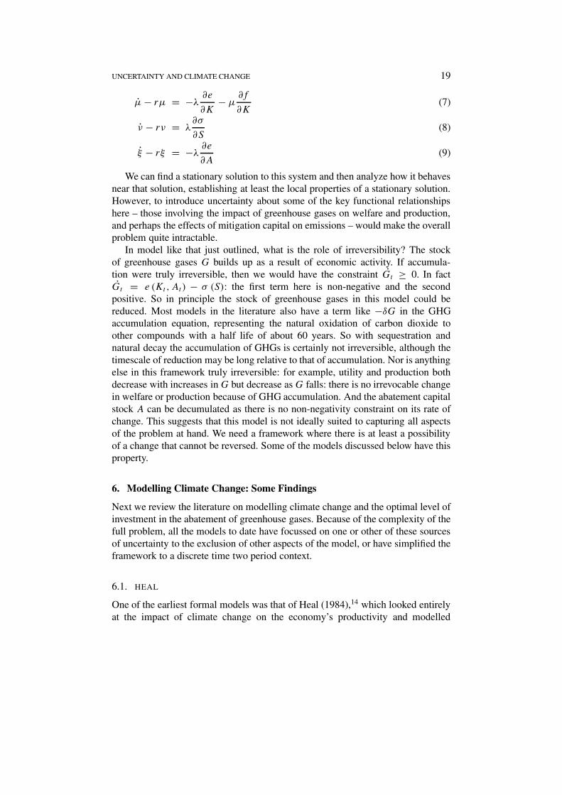
We can find a stationary solution to this system and then analyze how it behavesnear that solution, establishing at least the local properties of a stationary solution.However, to introduce uncertainty about some of the key functional relationshipshere – those involving the impact of greenhouse gases on welfare and production,and perhaps the effects of mitigation capital on emissions – would make the overallproblem quite intractable.

In model like that just outlined, what is the role of irreversibility? The stockof greenhouse gases G builds up as a result of economic activity. If accumula-tion were truly irreversible, then we would have the constraint Gt ≥ 0. In factGt = e (Kt , At ) − σ (S): the first term here is non-negative and the secondpositive. So in principle the stock of greenhouse gases in this model could bereduced. Most models in the literature also have a term like −δG in the GHGaccumulation equation, representing the natural oxidation of carbon dioxide toother compounds with a half life of about 60 years. So with sequestration andnatural decay the accumulation of GHGs is certainly not irreversible, although thetimescale of reduction may be long relative to that of accumulation. Nor is anythingelse in this framework truly irreversible: for example, utility and production bothdecrease with increases in G but decrease as G falls: there is no irrevocable changein welfare or production because of GHG accumulation. And the abatement capitalstock A can be decumulated as there is no non-negativity constraint on its rate ofchange. This suggests that this model is not ideally suited to capturing all aspectsof the problem at hand. We need a framework where there is at least a possibilityof a change that cannot be reversed. Some of the models discussed below have thisproperty.

6. Modelling Climate Change: Some Findings

Next we review the literature on modelling climate change and the optimal level ofinvestment in the abatement of greenhouse gases. Because of the complexity of thefull problem, all the models to date have focussed on one or other of these sourcesof uncertainty to the exclusion of other aspects of the model, or have simplified theframework to a discrete time two period context.

6.1. HEAL

One of the earliest formal models was that of Heal (1984),14 which looked entirelyat the impact of climate change on the economy’s productivity and modelled


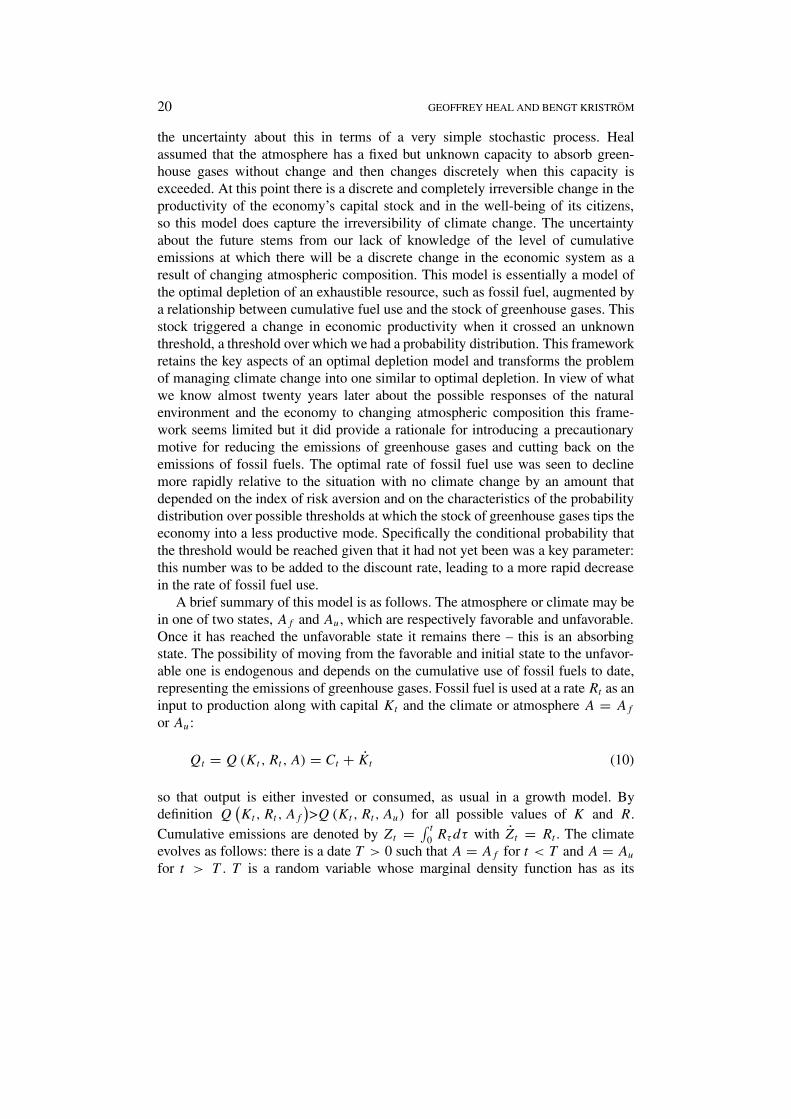
the uncertainty about this in terms of a very simple stochastic process. Healassumed that the atmosphere has a fixed but unknown capacity to absorb green-house gases without change and then changes discretely when this capacity isexceeded. At this point there is a discrete and completely irreversible change in theproductivity of the economy’s capital stock and in the well-being of its citizens,so this model does capture the irreversibility of climate change. The uncertaintyabout the future stems from our lack of knowledge of the level of cumulativeemissions at which there will be a discrete change in the economic system as aresult of changing atmospheric composition. This model is essentially a model ofthe optimal depletion of an exhaustible resource, such as fossil fuel, augmented bya relationship between cumulative fuel use and the stock of greenhouse gases. Thisstock triggered a change in economic productivity when it crossed an unknownthreshold, a threshold over which we had a probability distribution. This frameworkretains the key aspects of an optimal depletion model and transforms the problemof managing climate change into one similar to optimal depletion. In view of whatwe know almost twenty years later about the possible responses of the naturalenvironment and the economy to changing atmospheric composition this frame-work seems limited but it did provide a rationale for introducing a precautionarymotive for reducing the emissions of greenhouse gases and cutting back on theemissions of fossil fuels. The optimal rate of fossil fuel use was seen to declinemore rapidly relative to the situation with no climate change by an amount thatdepended on the index of risk aversion and on the characteristics of the probabilitydistribution over possible thresholds at which the stock of greenhouse gases tips theeconomy into a less productive mode. Specifically the conditional probability thatthe threshold would be reached given that it had not yet been was a key parameter:this number was to be added to the discount rate, leading to a more rapid decreasein the rate of fossil fuel use.

A brief summary of this model is as follows. The atmosphere or climate may bein one of two states, Af and Au, which are respectively favorable and unfavorable.Once it has reached the unfavorable state it remains there – this is an absorbingstate. The possibility of moving from the favorable and initial state to the unfavor-able one is endogenous and depends on the cumulative use of fossil fuels to date,representing the emissions of greenhouse gases. Fossil fuel is used at a rate Rt as aninput to production along with capital Kt and the climate or atmosphere A = Af

or Au:

Qt = Q(Kt, Rt, A) = Ct + Kt (10)

so that output is either invested or consumed, as usual in a growth model. Bydefinition Q

(Kt,Rt , Af

)>Q(Kt, Rt, Au) for all possible values of K and R.

Cumulative emissions are denoted by Zt = ∫ t

0 Rτdτ with Zt = Rt . The climateevolves as follows: there is a date T > 0 such that A = Af for t < T and A = Au

for t > T . T is a random variable whose marginal density function has as its


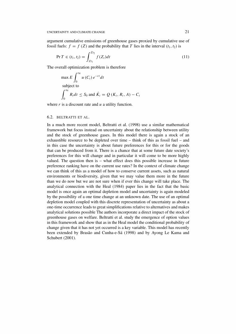
argument cumulative emissions of greenhouse gases proxied by cumulative use offossil fuels: f = f (Z) and the probability that T lies in the interval (t1, t2) is

PrT ∈ (t1, t2) =∫ Zt2

Zt1

f (Zt)dt (11)

The overall optimization problem is therefore

maxE

∫ ∞

0u (Ct) e

−rt dt

subject to∫ ∞

0Rtdt ≤ S0 and Kt = Q(Kt, Rt , A) − Ct

where r is a discount rate and u a utility function.

6.2. BELTRATTI ET AL.

In a much more recent model, Beltratti et al. (1998) use a similar mathematicalframework but focus instead on uncertainty about the relationship between utilityand the stock of greenhouse gases. In this model there is again a stock of anexhaustible resource to be depleted over time – think of this as fossil fuel – andin this case the uncertainty is about future preferences for this or for the goodsthat can be produced from it. There is a chance that at some future date society’spreferences for this will change and in particular it will come to be more highlyvalued. The question then is – what effect does this possible increase in futurepreference ranking have on the current use rates? In the context of climate changewe can think of this as a model of how to conserve current assets, such as naturalenvironments or biodiversity, given that we may value them more in the futurethan we do now but we are not sure when if ever this change will take place. Theanalytical connection with the Heal (1984) paper lies in the fact that the basicmodel is once again an optimal depletion model and uncertainty is again modeledby the possibility of a one time change at an unknown date. The use of an optimaldepletion model coupled with this discrete representation of uncertainty as about aone-time occurrence leads to great simplifications relative to alternatives and makesanalytical solutions possible The authors incorporate a direct impact of the stock ofgreenhouse gases on welfare. Beltratti et al. study the emergence of option valuesin this framework and show that as in the Heal model the conditional probability ofchange given that it has not yet occurred is a key variable. This model has recentlybeen extended by Brasão and Cunha-e-Sá (1998) and by Ayong Le Kama andSchubert (2001).


6.3. KELLY AND KOLSTAD

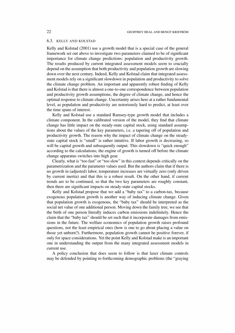
Kelly and Kolstad (2001) use a growth model that is a special case of the generalframework set out above to investigate two parameters claimed to be of significantimportance for climate change predictions: population and productivity growth.The results produced by current integrated assessment models seem to cruciallydepend on the assumption that both productivity and population growth are slowingdown over the next century. Indeed, Kelly and Kolstad claim that integrated assess-ment models rely on a significant slowdown in population and productivity to solvethe climate change problem. An important and apparently robust finding of Kellyand Kolstad is that there is almost a one-to-one correspondence between populationand productivity growth assumptions, the degree of climate change, and hence theoptimal response to climate change. Uncertainty arises here at a rather fundamentallevel, as population and productivity are notoriously hard to predict, at least overthe time spans of interest.

Kelly and Kolstad use a standard Ramsey-type growth model that includes aclimate component. In the calibrated version of the model, they find that climatechange has little impact on the steady-state capital stock, using standard assump-tions about the values of the key parameters, i.e. a tapering off of population andproductivity growth. The reason why the impact of climate change on the steady-state capital stock is “small” is rather intuitive. If labor growth is decreasing, sowill be capital growth and subsequently output. This slowdown is “quick enough”according to the calculations; the engine of growth is turned off before the climatechange apparatus switches into high gear.

Clearly, what is “too fast” or “too slow” in this context depends critically on theparametrization and the parameter values used. But the authors claim that if there isno growth in (adjusted) labor, temperature increases are virtually zero (only drivenby current inertia) and that this is a robust result. On the other hand, if currenttrends are to be continued, so that the two key parameters are roughly constant,then there are significant impacts on steady-state capital stocks.

Kelly and Kolstad propose that we add a “baby tax” to a carbon-tax, becauseexogenous population growth is another way of inducing climate change. Giventhat population growth is exogenous, the “baby tax” should be interpreted as thesocial net value of one additional person. Moving down the family tree, we see thatthe birth of one person literally induces carbon emissions indefinitely. Hence theclaim that the “baby tax” should be set such that it incorporate damages from emis-sions in the future. The welfare economics of population growth raises profoundquestions, not the least empirical ones (how is one to go about placing a value onthose yet unborn?). Furthermore, population growth cannot be positive forever, ifonly for space considerations. Yet the point Kelly and Kolstad make is an importantone in understanding the output from the many integrated assessment models incurrent use.

A policy conclusion that does seem to follow is that laxer climate controlsmay be defended by pointing to forthcoming demographic problems (the “graying


Europe” is a case in point). Bringing uncertainty proper into a model with similarcharacteristics may turn the Kelly and Kolstad argument on its head, at leastaccording to Pizer (1998), to which we now turn.

6.4. PIZER

Pizer’s (1998) model allows for many different states of nature, includes econo-metric estimates of key technology and preference parameters (rather than “bestguesses”) and has consistent welfare aggregation of uncertain utilities.15 Arepresentative consumer maximizes a Von Neumann-Morgenstern utility func-tion within a stochastic growth model that has a climate component (from theDICE-model). The utility function has constant relative risk aversion and a fixedutility discount rate is assumed. Production (Cobb-Douglas technology) is a func-tion of capital and augmented labor. Net labor productivity is related to thecosts of controlling damages; essentially a quadratic damage cost function isused (for temperature changes less than about 10 degrees Celsius). Exogenouslabor productivity is a random walk (in logarithms). This formulation impliesthat exogenous productivity growth slows down over time (and begins at about1.3%, according to Pizer’s estimates). Population growth, which is exogenous,is modelled in a similar manner. Emissions are proportional to BAU-output andendogenous emission reductions. A simple climate module completes the model.

The empirical model encompasses a rich set of different uncertainties,including uncertainty utility, cost and technology parameters, as well as parametersdescribing the development of carbon dioxide in the atmosphere. The econometricmodel combines data with a prior distribution over the parameters, i.e. Bayesiananalysis is used. Data from the national accounts covering the US over the period1952-1992 are used to estimate structural parameters, such as time preference,productivity growth and capital share. In this way, the marginal distribution of eachparameter is obtained, which then provides a coherent way of describing parameteruncertainty.

According to Pizer (1998), the impact of general parameter uncertainty showsmost clearly in the long-run; short-run responses are rather similar, whether or notuncertainty is included. He finds that productivity slowdown encourages stricteroptimal regulation, thus reversing the Kelly and Kolstad conclusion. The expla-nation is, according to Pizer, related to how damages are discounted. Slowerproductivity growth tends to depress interest rates (this follows from the Eulerequation). Consequently, if damages are discounted with a lower discount rate, thepresent value of those damages is higher. Thus, from the point of view of “today”the value of avoiding climate damages in the future gets a relatively higher value.

A puzzling result is that if best-guessed parameter values are imposed, thisproduces a path with lower welfare, compared to the case when uncertainty isexplicitly handled. It appears as if the stricter policy associated with uncertaintycase wins more often than it loses, because the gains from avoiding large losses in


a bad state of the world, outweigh the cost of overcompliance in the good states.This is related to Weitzman’s (1974) price versus quantity result. In Pizer’s (1998)model, the marginal benefit curve is relatively flat compared to the marginal costcurve. If follows from Weitzman (1974) that taxes tend to give lower efficiencylosses, compared to a quantity instrument, in such settings (see Dasgupta (1982)for a useful discussion of instrument choice under uncertainty). The propositionthat tax instruments are to be preferred in climate policy has some general support,see e.g. Toman (2001).

Finally, we note that the model appears to be rather sensitive to climate para-meters. This seems, at least, to be true for the original DICE-model and there aregood reasons to believe that this conclusion carries over. An important parameteris the climate sensitivity, which is set to 2.9 degrees Celsius in the standard DICEmodel. It is allowed to vary in Pizer’s model according to a uniform 5-point distri-bution on the interval (1.5–4.5). Keller et al. (2000) illustrate the key role played bythis parameter in their analysis of potential thermohaline collapse, within a slightlymodified DICE-model.

6.5. IRREVERSIBILITY, OPTION VALUES AND PRECAUTION

There is a group of papers that focus on the modeling of irreversibility and thepossibility of an option value, as discussed above. These include Fisher and Narain(2002), Gollier et al. (2000), Kolstad (1996a, b), Pindyck (2000), Ulph and Ulph(1997), and several others.16 We group them together because they have manypoints in common. In an interesting and provocative paper, Ulph and Ulph focusdirectly on the question of whether there are option values associated with thepreservation of the existing climate system. As already noted, the preconditionsnecessary for the existence of an option value seem to be satisfied in the contextof climate change. We expect to learn about the costs of climate change and aboutthe costs of avoiding it over the next decades. And we expect that some of thedecisions that we could take will have consequences that are irreversible. These arethe hallmarks of decisions that give rise to option values associated with conserva-tion – the pioneering studies by Arrow and Fisher (1974) and by Henry (1974a, b)have exactly these properties. But although these conditions are necessary for theexistence of option values they are not sufficient. Kolstad uses a similar frameworkand asks a similar question: it is to his paper that we owe the observation that thereis another possible real option value at work here. If substantial sunk costs mustbe incurred to begin the process of abating greenhouse gas emission and avoidingor minimizing climate change, if the return to this investment is the avoidanceof climate change, and if we learn about the value of this over time, then thereis also a real option value associated with postponing investment in greenhousegas abatement. So in Kolstad’s model, which like the general model above hasboth GHG accumulation and investment in abatement capital, there are two optionvalues acting in opposition in this framework. Both Ulph and Ulph and Kolstad


use a result of Epstein’s (1980) which can be applied to the analysis of learningand option values: this is in some sense a generalization of the famous papers byHenry and Arrow and Fisher and gives conditions that are necessary and sufficientfor the existence of option values. Ulph and Ulph and Kolstad give conditionsunder which there are option values associated with the preservation of the existingclimate regime, and it is clear that these conditions are quite restrictive – althoughthere is no suggestion that they are necessary. Ulph and Ulph, Kolstad and Fisherand Narain specialize to discrete time two or three period models in order to findsolutions. In the Epstein result, and some others based on it, the third derivative ofthe utility function is a key variable: an inequality involving this third derivativedetermines whether or not there is an option value. In other problems involvingchoice under uncertainty the third derivative of the utility function has also beena key variable and Gollier et al. (reviewed below) give this an intuitive interpreta-tion. Fisher and Narain have a more encouraging outcome: in their formulation theindex of relative risk aversion is the important parameter. Their paper has a goodsummary of earlier results in its introduction, and makes an interesting observationabout irreversibility of investment in abatement capital: they note that there are twopossible interpretations here. One is to measure irreversibility by the durability ofthe capital, as in the Kolstad paper: the other is to define investment in abatementcapital as irreversible if that capital is “non-shiftable” in the terminology of optimalgrowth theorists (Arrow and Kurz 1970) – i.e. if it cannot be consumed or used insome other sector. Fisher and Narain note that the consequences of irreversibilityof abatement investment depend on which of these definitions one uses, and thatthey are somewhat more intuitive if one uses the conventional optimal growth inter-pretation of irreversibility. Fisher and Narain also compare results with exogenousand endogenous climate risks – i.e. in the cases where the probability distribution ofdamages due to greenhouse gas accumulation is affected by the stock of greenhousegases. The other papers take this distribution to be exogenous.

Pindyck works with the most general of the models in this category, usinga multi-period stochastic optimal growth model. Not surprisingly he gives onlynumerical solutions, and offers a very appropriate summary of the issues and ofwhy it proves difficult to reach firm conclusions about the nature and directionof option values. He comments that “I have focused largely on a one-time policyadoption to reduce emissions of a pollutant. If the policy imposes sunk costs onsociety, and if it can be delayed, there is an opportunity cost of adopting thepolicy now rather than waiting for more information. This is analogous to theincentive to wait that arises with irreversible investment decisions. In the caseof environmental policy, however, this opportunity cost must be balanced againstthe opportunity “benefit” of early action – a reduced stock of pollutant that mightdecay only slowly, imposing irreversible costs on society.” He goes on to makecomments that are specific to his particular model structure, but are neverthelessenlightening on how things work in this context. “In the simple models presentedin this paper, an increase in uncertainty, whether over future costs and benefits of


reduced emissions, or over the evolution of the stock of pollutant, leads to a higherthreshold for policy adoption. This is because policy adoption involves a sunk costassociated with a discrete reduction in the entire trajectory of future emissions,whereas inaction over any small time interval only involves continued emissionsover that interval. . . . The validity of this result depends on the extent to whichenvironmental policy is indeed irreversible, in the sense of involving commitmentsto future flows of sunk costs.” An interpretation of this seems to be that if policiesare flexible and do not necessarily involve commitments to their continuation overlong periods, then the asymmetry that he finds would vanish and there would nolonger be a tendency of greater uncertainty to favor a more cautious adoption ofpolicies. This in turn suggests that we need to spend more time than we havethinking about the design of policies in this area, and in particular ensuring thatthey are flexible and permit changes in response to new information.

Gollier et al. (2000) tackle a similar set of questions but from a slightly differentperspective. They use the idea of the “precautionary principle” as the organizingtheme of their work. They quote the 1992 Rio Declaration (Article 15) as a state-ment of this: “where there are threats of serious and irreversible damage, lack offull scientific certainty shall not be used as a reason for postponing cost-effectivemeasures to prevent environmental degradation.” The reference to scientific uncer-tainty here implies, for the authors, the possible resolution of this uncertainty byresearch and learning. Most economists, if asked to think of a justification for thisprinciple, would probably couch it in terms of learning, irreversibilities and optionvalues, so intuitively we think we two are related. Gollier et al note that in factthe precautionary principle can be given a formal justification without invokingirreversibilities, just assuming a stock damage effect and possible learning overtime. They consider two economies that are identical except in the way the infor-mation structure evolves over time. They then say that the precautionary principleholds if in the economy in which more information becomes available over time wedo not invest less in damage prevention: for them the essence of the precautionaryprinciple is a positive relationship between information acquisition and precaution.They note, as in most of the models already discussed, that there are two contra-dictory effects. One is that we invest less in prevention in the economy which maylearn more because this investment may be inefficient: when we know more wemay be able to choose better investments. They describe this as the “learn thenact” strategy. The opposing tendency is generated by the fact that if we follow thisstrategy then the risk that society faces in the future will be greater. The principleresult of the Gollier et al paper is that the balance between these two effects dependson the shape of the utility function and in particular on whether or not societyshows “prudence”. Prudence is equivalent to a positive third derivative of the utilityfunction: a prudent person increases her savings in the face of an increase in therisk associated with future revenues (Kimball 1990). For a class of utility functionsGollier et al. give necessary and sufficient conditions for the precautionary prin-ciple to hold, but note that outside of this class there are no general results. They


then go on to consider the relationship between the precautionary principle andirreversibility.

In a very interesting paper, Carpenter, Ludwig and Brock (1999) set out a radi-cally different approach. Their paper is not in fact about climate change: the titleis “Management of Eutrophication for Lakes Subject to Potentially IrreversibleChange.” The problem addressed can be summarized as follows. In a farmingregion, such as the mid West of the USA, phosphorous P is applied as a fertilizerto the land around a lake and some of it runs from there into the lake. In sufficientconcentration in the lake, it can cause a change in the biological state of the lake,to a potentially stable state of eutrophication in which the lake is unproductive formost human uses. So eutrophication is irreversible. The response to P concentrationis highly non-linear and the concentration of P depends not only on the runoff butalso on temperature and rainfall, which are random. How should we manage therunoff of P over time to maximize the expected discounted value of benefits netof the costs of P mitigation? This problem has all the structure of the climateproblem: indeed as we said in the first discussion of irreversibilities, the climatesystem is a complex nonlinear dynamical system that may change regime underhuman perturbation. This is exactly what Carpenter, Ludwig and Brock modeltreats, though for a more finite problem. They talk about the concept of resilience,“the capacity of a non-linear system to remain within a stability domain. . . .” Thisconcept has been widely used in mathematical ecology. They model the dynamicsof the interacting lake and agricultural systems as a nonlinear dynamical systemwith several different locally stable states, one of which is highly unattractive.Avoiding this state is costly, so that there are trade-offs to be made. And thestochasticity of the weather means that the problem has to be seen in probabilisticterms. An interesting conclusion that these authors reach is the following: “Animportant lesson from this analysis is a precautionary principle. If P inputs arestochastic, lags occur in implementing P input policy, or decision makers are uncer-tain about lake response to altered P inputs, then P input targets should be reduced.In reality, all of these factors – stochasticity, lags, uncertainty – occur to somedegree. Therefore, if maximum economic benefit is the goal of lake management,P input levels should be reduced below levels derived from traditional limnologicalmodels. The reduction in P input targets represents the cost a decision maker shouldbe willing to pay as insurance against the risk that the lake will recover slowly ornot at all from eutrophication. This general result resembles those derived in thecase of harvest policies for living resources subject to catastrophic collapse.” Theygo on to say that “We believe that the precautionary principle that emerges fromour model applies to a wide range of scenarios in which maximum benefit is soughtfrom an ecosystem subject to hysteretic or irreversible changes.”

The model of Carpenter and coauthors seems very readily applicable to climatechange: as we have noted above, the climate system may in some respects beirreversible and in some aspects it can be modelled as a dynamical nonlinearsystem with several basins of attraction – this is the way in which climate modelers


represent the alternative states of thermohaline circulation and the Gulf Stream.And even if we are dealing with aspects of the climate system that do not havethis characteristic, the changes in ecosystems driven by the climate are very likelyto have exactly the characteristics considered by Carpenter, Ludwig and Brock(1999). So considering the climate system and its ecological consequences, whichis what is relevant from the social and economic perspective, this seems like aproductive framework. In this context the precautionary principle enunciated byCarpenter, Ludwig and Brock (1999) is thought-provoking. Little as clear as thishas emerged from the other models cited here. Their result is suggestive of thecertainties of the early papers of Arrow-Fisher and Henry. In part this probablyreflects the advantages of modelling the system’s dynamics explicitly, and perhapsalso reflects the fact that the Carpenter et al. omits – quite legitimately in theircontext – one issue that is central to the work of Kolstad, Ulph and Ulph andothers cited above. This is the need to make a durable investment in greenhousegas abatement. In controlling the runoff of P there is no equivalent: the applicationof P can be controlled on a day-to-day basis and can be decreased without priorinvestments in capital equipment. In Pindyck’s terms, policy is flexible. It wouldbe of great interest to know whether the Carpenter, Ludwig and Brock results wouldsurvive the need for investment to control P runoff.

7. Climate Change and Risk Management

Next we discuss the institutional framework with which we could manage therisks arising from climate change. Economists have two standard models of risk-allocation in a market economy. The more general is that of Arrow and Debreu,in which agents trade “contingent commodities”. The alternative is the model ofinsurance via risk-pooling in large populations. Neither can address fully all theparticular characteristics of global environmental risks. In particular, both assumethe risks to be known in some sense, and to be exogenous.

In the Arrow-Debreu framework there is a set of “states of nature.” The probabi-lities of these being realized are exogenous and these states represent the sourcesof uncertainty. Classically one thinks of events such as earthquakes and meteorstrikes. Their occurrences are assumed to be exogenous to the economic system,and not affected by economic activity. Agents in the economy are allowed totrade commodities contingent on the values of these exogenous variables. Theseare called “state-contingent commodities”. With a complete set of markets forstate-contingent commodities, the first theorem of welfare economics holds foreconomies under uncertainty: an ex-ante Pareto efficient allocation of resources canbe attained by a competitive economy with uncertainty about exogenous variables.

Arrow showed that efficiency can in fact be attained by using a mixture ofsecurities markets and markets for non-contingent commodities, so that a completeset of contingent commodity markets is not required. This observation provides anatural and important role for securities markets in the allocation of risk-bearing.


The securities used are contracts that pay one unit if and only if a particular stateoccurs. While the contingent contract approach is in principle all-inclusive andcovers most conceivable cases of uncertainty, in practical terms there are caseswhere it can be impossible to implement. It can be very demanding in terms of thenumber of markets required. For example, if agents face individual risks (i.e., riskswhose probabilities vary from individual to individual), then in a population of100 similar agents each of whom faces two possible states, the number of marketsrequired would be 2100 (see Chichilnisky and Heal 1998). The number of marketsrequired is so large as to make the contingent contract approach unrealistic.

The use of insurance markets for pooling risks is a less general but more prac-tical alternative. This requires that populations be large and that the risks be small,similar and statistically independent. The law of large numbers then operates andthe frequency of occurrence of an insured event in a large sample of agents approx-imates its frequency in the population as a whole. To be precise, assume that each ofN people faces a loss of L with probability π , and an insurance company insuresthem against this loss. Assume the losses are independent. The loss rate for thepopulation is the expected claims divided by the total insurance offered. A 95%confidence interval for this is just π ±

√π[1−π%]√

Nso that the loss rate converges

to the actuarial probability as the population increases. There is thus a role forinsurance companies to act as intermediaries and pool large numbers of similarbut statistically independent risks. In so doing they are able via aggregation andthe use of the law of large numbers to neutralize the risks faced by many similaragents. The main references on this are Arrow and Lind (1970) and Malinvaud(1972, 1973).

The insurance approach is at a disadvantage when risks are correlated. Whenlarge numbers are likely to be affected at once, risk-pooling will not work. Howeverit does have the advantage relative to the contingent market approach of econom-izing dramatically on the number of markets needed. In the above example, onlytwo mutual insurance contracts and 2809 securities would be needed instead of2100 contingent contracts.

7.1. UNKNOWN RISKS

When risks are allocated by trading state-contingent commodities securities, or byrisk-pooling and insurance, it is very important that agents know, or believe thatthey know, the relative frequencies of the states of nature, at least approximately.This is obvious when trading insurance contracts. The actuarial calculations neededto set insurance premia can only be performed if the parties believe that the relativefrequencies of the insured events are approximately known.

In the Arrow-Debreu approach, it suffices to think of agents maximizingexpected utility to appreciate the need for them to know, or at least behave as ifthey know, the relative frequencies of exogenous states. These frequencies are theweights placed on their utilities from state-dependent consumption. The point is


simple: if agents can not assign relative frequencies then their preferences are notwell-defined and they cannot act to maximize expected utility.

As we have noted above, in the context of such risks as climate change, ozonedepletion and in particular biodiversity loss this is probably much too demanding.Agents, even experts, do not know the frequencies of different states, and recognizethat they do not know them. The reviews by Roughgarden and Schneider (1999)and the IPCC TAR of expert judgements on the impact of climate changes empha-sizes this. They recognize that there are several different opinions about what theseare, but feel unable to choose definitively between these alternatives. In such acase, it is natural to think of the frequency distribution over environmental changesas a state of the world, a risk, in the Savage sense: we do not know what valueit will assume, and whatever value this is, it affects economic activity. Ignorancethen assumes the role of a collective risk, and can be treated by the use of state-contingent markets.

Chichilnisky and Heal (1993, 1998) formalize this type of situation in a simplegeneral equilibrium model. Each agent faces the risk of being in one of severalstates (e.g. healthy or sick, productive or unproductive, environmentally impover-ished or not, etc.). No-one knows what will be the true frequency distribution ofaffected agents. A probability is assigned to each of several frequency distributionsthought to be possible. A typical probability distribution of this type might state forexample that there is a 10% chance that 90% of the population will be harmed byglobal warming, a 25% chance that 50% of the population will be harmed, etc. Theprobability distribution over alternative frequency distributions may be differentfrom individual to individual. Again this is consistent with the expert opinions onclimate change summarized by Roughgarden and Schneider.

In this framework, we have two levels of uncertainty. The first level of uncer-tainty is collective: what is the distribution of agents who are harmed in theeconomy? Will 90% be harmed, or only 30%? This is a question about theaggregate incidence of the phenomenon over the population as a whole. This riskrepresents or arises from our lack of knowledge of the phenomena at stake.

The second level of uncertainty is individual: it is uncertainty about whether agiven agent is harmed or not by climate change. It devolves about questions suchas: given that 90% of the population will be harmed or environmentally impover-ished, will a particular agent be harmed or not? The issue here is: contingent ona particular overall incidence of the phenomenon, who are the agents who will beaffected?

Chichilnisky and Heal (1998) suggests an institutional structure which usestwo types of financial instruments which are tailored to these two aspects ofthe problem. These can lead to efficient allocation in the face of such risks.One instrument is a mutual insurance contract to deal with the risks faced byagents or communities contingent on each possible distribution of harmful effectsworldwide. A mutual insurance contract is an agreement between parties subjectto similar risks that those who are harmed will be compensated by the others.


Examples are agricultural cooperatives of the type recorded in Europe at least sincethe fifteenth century, and the nineteenth century U.K. workers’ associations andfriendly societies. These involved agreements between a group of workers that ifone were sick and unable to work, he or she would be compensated by the others.In the present context, one could think of groups of communities subject to thepossible impact of climate change, with those unharmed compensating the others.Making the terms of such a mutual insurance contract contingent on the distri-bution of harmful effects worldwide means that there is a different compensationagreement between the parties for each possible aggregate distribution of harmfuleffects. To know what compensation is due in any particular case, the parties havefirst to assess the distribution of harmful effects globally, and on the basis of thisdecide which mutual insurance contract to apply.

Having dealt with individual risks by mutual insurance, we still face collectiverisks. We need statistical securities to deal with these collective risk induced byuncertainty about the overall distribution of adverse effects. Arrow securities aredefined as securities that pay one dollar if and only if a particular state of theworld occurs. Statistical securities pay one dollar if and only if there is a particularfrequency of affected parties in the population, i.e., if and only if there is a partic-ular statistical state, a state of the economy with specified statistical characteristics.As already noted, the incidence of impacts on the population as a whole is beingtreated as a “state of the world” in the Arrow-Debreu sense. We treat each possibledistribution of adverse affects as a distinct collective state (called a statistical state),and use securities markets to enable parties to transfer wealth between these states.One statistical security is needed for each possible distribution of adverse effectsworldwide, because to attain Pareto efficiency each separate state must be coveredby a security. The core of the results in Chichilnisky and Heal is that with unknownrisks we can trade securities contingent on statistical states and this can allow theuncertainty introduced by alternative probability distributions to be fully hedged.

There are two features of the results which are of general interest. One isthe development of a framework for achieving efficient allocations in the faceof uncertain individual risks. Given rapid changes in technology with potentiallyfar-reaching environmental impacts and health effects, the problem of providinginsurance against such risks is particularly important. It is a matter of very activeconcern in the insurance industry. The second interesting feature is the way acombination of securities markets and insurance markets can be used to provide arelatively simple institutional structure for dealing with unknowable risks. Currenttrends in the securitization of certain risks are consistent with this analysis. InChichilnisky and Heal (1998) it is shown that under certain simplifying assump-tions this framework will lead to an efficient allocation of risks in a competitivegeneral equilibrium model. Subsequently Klimpel and Requate (2000) generalizedthese results.

Another radically different approach to the fact that risks are unknown hasbeen explored by Henry and Henry (2000). A central feature of their analysis is


an explicit recognition that we do not have a complete probability distributionover possible climate change events and consequences. There may be changes andconsequences that we have not yet envisaged. In such a case the probabilities thatwe assign to the events about which we do have information must sum to less thanone, to leave room for the unknown events. So what we have to work with is ameasure on the set of known possible events, whose integral is less than one. Andeven on the events about which we know something, it is possible that our beliefscan not be described by a measure that satisfies the conditions that are needed for itto be a part of a probability distribution: they may be too imprecise for this. Imple-menting these observations, which seem quite compelling in the climate changecontext, requires that we work within the framework of non-additive probabilitieson the state space. The prerequisites for following such arguments in detail aremore demanding than those for most of the literature that we have reviewed, so wewill merely mention this approach, which to us looks particularly promising, andnote that it provides another context in which one can formalize a precautionaryprinciple. Precautionary behavior is now motivated in part by the possibility ofevents and outcomes that we cannot characterize. One is reminded of Hamlet’sthoughts on death:

The dread of something after deathThat undiscovered country from whose bourn

No traveller returns, puzzles the willAnd makes us rather bear those ills we have

Than fly to others that we know not of

Shakespeare seems to have anticipated the precautionary principle here.

7.2. ENDOGENOUS RISKS

The risks we face in environmental change are not only not well known: theyare also not exogenous. Almost by definition, they are endogenous and are deter-mined by our behavior. In effect we both create states of nature and determinethe probability distributions over these. By creating the states of nature we meanthat human actions make possible states of the planetary systems that would nototherwise occur. For example, human actions are leading to patterns of land useand of species diversity that certainly would not have occurred without our actions:intensive agriculture is a form of land use that would not have arisen without humanactivity, and the transportation of exotic species, a major threat to biodiversity, isalso uniquely a product of the patterns of human activity.

In all of the classical models of risk management discussed above, it is assumedthat the risks faced are exogenous: that is, they are not affected by human actions.At the microeconomic level, the fact that human actors can affect the probabilitiesof the risks that they face has long been recognized as a serious problem for theoperation of insurance markets, under the title of moral hazard. The focus in this


literature has been on the fact that offering insurance to a person may lead herto behave in a way that alters the risk that she faces. Deductibles and co-insurancehave been the recommended solutions to the problems that this creates for attainingan efficient allocation of the risks – although they do not lead to a first best outcome.

More recently there has been a literature on endogenous uncertainty in a generalequilibrium context.17 This literature has addressed the issues that arise whenagents are uncertain about the values of endogenous variables. A good exampleis provided by uncertainty about the values of stock prices or of exchange rates.The natural question is whether we can use the device of trading state-contingentcontracts to handle this uncertainty. In this case the contracts would have to becontingent on the prices about which agents are uncertain. These have been termedprice contingent contracts, or PCSs. It is possible to construct an institutionalframework within which trading price-contingent contracts will lead to a fully effi-cient insurance of the risks associated with uncertainty about prices, and this leadsquite naturally to a general equilibrium theory of the role and pricing of derivativesecurities. The framework involves trading securities contingent on the prices thatare realized at equilibrium in a market for PCSs that operates before the market forgoods and services opens. Heal (1995) considers an exchange economy augmentedby the possibility of trading price contingent securities which pay a specified sumif and only if the equilibrium price vector assumes a specified value. Prices playthe role played by “states of nature” in the Savage framework, so the determinationof the state is endogenous. Agents have expectations about possible prices, andtrade price contingent securities to insure price risks. They use these securities toexchange income in price states in which they are well off for income in states inwhich they are badly off. Before an equilibrium price emerges agents trade thesesecurities, shifting income across price states. This changes their endowments inthe exchange economy, which now become price contingent.

How does this relate to the endogeneity of environmental uncertainty? Thesimilarity is that the possible environmental states and their probabilities are deter-mined by human actions, indeed in part by the equilibrium of our economicsystem and the environmental impacts of the selected activities. The analogywith endogenous price uncertainty suggests an approach based on trading secur-ities contingent on the environmental states before these are realized. This wouldinvolve markets on which we trade securities that pay dependent on the amount ofclimate change and its location and timing, or on the state of the ozone layer in agiven year, or on the state of biodiversity. So we would have markets for climatebonds, or ozone bonds or biodiversity bonds. In case this sounds exotic, note thatWall Street already trades hurricane bonds, earthquake bonds, catastrophe futures,Act-of-God bonds and a few others. All of these exist for the purpose of shiftingthe risks associated with environmental phenomena.

How would such instruments work and what would they contribute? Thepayoffs from these bonds would shift endowments around in a way that dependedon the state of the environment, making the distribution of endowments in the


rest of the economic system contingent on the state of the environment, just asPCSs make the distribution of endowments contingent on the vector of equilib-rium prices in a general equilibrium model with price uncertainty. Given a stateof the environment and a distribution of endowments resulting from environment-contingent bonds, trade would then occur as normal and would lead under the rightconditions to an efficient allocation of resources.

By following the arguments in Heal (1995), we can show that this system hasa competitive equilibrium at which all agents are insured to precisely the degreethat they want against the risks associated with not knowing what the states ofthe environment and economy will be. The markets for securities contingent on thestate of the environment and the economy will provide an efficient allocation of therisks arising from environmental uncertainty. The kinds of markets we have in mindhere are exemplified by markets in which one can insure against a certain levelof climate change and its economic consequences, captured in the model by theenvironmental state and the price vector. Such markets do not currently exist, butmarkets for securities continent on the state of the environment do exist, in the formof hurricane bonds and weather swaps. There is currently a proposal to introducea tradable index of the state of the ENSO (El Nino-Southern Oscillator) cycle,which would be a move closer to a general security whose payoff depends on thestate of the climate system. Note that although these markets would allocate effi-ciently the risks of environmental change, they would not lead to a Pareto efficientallocation, as the externalities associated with behavior that affects the climate arenot corrected. That would require a separate set of policy instruments, such as theclassical corrective taxes and subsidies or the use of tradable permits. In the formalmodel referred to here, there is no explicit connection between the acts of any oneagent and the probabilities of the states so that these externalities are not addressed.However, if corrective taxes or equivalents (such as permit markets) were in place,then the outcome of these markets would be a Pareto efficient allocation.

8. Conclusion

Climate change involves uncertainties in a breathtaking number of dimensions,including, but not limited to, the fields of natural science and economics. Thispaper tries to show why economic analysis that explicitly incorporates uncertaintygives some valuable insights into the policy issues raised by the possibility ofclimate change. True, even if the underlying problems were deterministic, thenthe economics of this issue would pose many interesting challenges, but formalanalysis of decision making under uncertainty must certainly play a dominant rolein any economic discussion about climate change policy.

A first point that we make may seem self-serving to non-economists, yet itsimportance is often overlooked in a discussion that gravitates too much towardsthe scientific uncertainties. Both empirical and theoretical studies show that weshould worry not only about disentangling nature’s true blueprint but also about


uncertainties that are intrinsic to the economic system, such as discount rates,growth rates and the rate of technological advance. After all, the engine of growthis a driver of climate change and understanding the relevant parts of the economicsystem should help us make better predictions. Our survey of some of the relevantempirical evidence does bring this point home rather forcefully.

There is a significant economic literature on irreversibilities, option values andthe value of flexibility, and this literature plays a dominant role in our discussions.A key insight from this literature is that option values have two dimensions: thereis a value of waiting for more information in order not to destroy irreversibly somenatural process, but there is also a value of waiting to invest scarce resources inabatement technology. While the relevant empirical evidence on option values isscarce, to say the least, economic theory gives some useful leads on where to lookfurther and why one needs to strike a balance between countervailing forces.

To this we must add the sobering fact that there are future unknown risksthat will require scarce economic resources. Somehow we need to find a balancebetween allocating resources to risks that are known today and to future unknownrisks. As Wildawsky (1988, p. 217) eloquently put it “Insofar as we today shouldconsider the welfare of future generations, our duty lies not in leaving them exactlythe social and environmental life we think they ought to have, but rather in makingit possible for them to inherit a climate of open choices. That is, in leaving behinda larger level of general fluid resources to be redirected as they, not we, seefit.” Climate policy that properly takes into account the value of flexibility andadaptation seems to be the most promising way of satisfying this recommendation.

Acknowledgement

We are grateful to Max Auffhammer, Claude Henry, Mark Machina and Art Smallfor valuable comments and suggestions on this paper.

Notes

1. An earlier review of the extent and nature of uncertainty in climate forecasting can be found inRoughgarden and Schneider (1999).

2. To be fair to the climate science community we should probably think of the change in temper-ature as a variation in the earth’s absolute temperature, which is about 280 degrees Kelvin, sothat we are looking at uncertainty that is only a couple of percentage points of the absolutetemperature. Mason (1995) provides a perspective on the development of climate modelling.Note that anthropogenic emissions are only a fraction of what is added each year in termsof carbon. This does not simplify the task of predicting the consequences for the climate ofhuman-made carbon reductions that are likely to be some fraction of current emissions.

3. Interestingly, the first two IPCC Assessment Reports did not discuss adaptation. This omis-sion has been attributed to political pressure from the environmental lobby. As the Columbiasociologist Steve Rayner has quipped, “Environmentalists don’t want to talk about adaptationfor the same reason Southern Baptists don’t want to talk about birth control,” i.e., out of concernthat the act of talking about these measures might be construed as an acceptance of the sinful


behavior leading to their necessity. See Kane and Shogren (2000) for a summary on adaption andmitigation arguments. They make the important point that adaption and mitigation are linked.Indeed, the Kyoto-protocol posits world-wide (but not global) mitigation efforts. Combiningmitigation and adaption, however, would seem to afford the same climate improvement at lessercost. They also note that attempts to ”assess risk levels solely in terms of natural science may bemisleading and costly; adaption and mitigation are endogenous to the integrated system . . .”

4. For a recent summary of the environmental economics literature on endogenous risk, see Crockerand Shogren (2003).

5. A numerical analysis of the economics of a potential collapse of the thermohaline circulationsystem, using a modified version of DICE (Nordhaus 1994), is in Keller, Tan, Morel, and Brad-ford (2000). An expanded version of this work that also include e.g. learning effects, arrives atthe same conclusion, namely that significant reductions of carbon emissions may be worthwhile.See Keller, K. , Bolker, B.M. and D.F. Bradford, ”Uncertain Thresholds and Economic OptimalGrowth”. www.princeton.edu/˜bradford/kellerbolker.pdf. This is to be compared with severalwell-known empirical models, DICE is an example, that predict rather modest costs of climatechange. More on this later in the paper.

6. The calculations that follow are taken from work in progress by Geoffrey Heal and Yun Lin,Columbia University.

7. If there is climate change, then income drops from I to Ij with probability pj , where clearlyIj ≤ I and

∑j pj ≤ 1. This can be weakened to allow an income drop on the average, in order

to include a possibility for income increases. With risk aversion, people would still be willing topay to avoid the change. Thanks to Mark Machina for pointing this out.

8. Because of the choice of functions for which the IRRA is constant, the ratio x/I is independentof the value of I , so that we do not need to think hard in choosing a value for I .

9. For an interesting review of the available evidence on the probabilities of loss from climatechange see Roughgarden and Schneider (1999), who take a range of expert opinions and fit asystematic probability density function to these. Geoffrey Heal is in the process of recomputingthis model with the probability-of-loss function given in Roughgarden and Schneider (1999).

10. As Arrow (1995, p. 16) points out, however: “When Ramsey was in a less moral mode he infact agreed [that the pure rate of time preference is positive]”. Arrow refers to Ramsey (1931,p. 291).

11. For a general discussion of these issues, see Heal (1998). Cline (1992) is an empirical study thatindicates the sensitivity of a choice to the discount rate.

12. Weitzman asks for a constant discount rate, although as Heal (1998) points out, the consumptiondiscount rate is not necessarily constant over the time spans considered (several centuries). Thisfollows from the Euler equation of a standard Ramsey problem. A slowing down of economicgrowth entails, for example, a lower consumption discount rate, if the utility discount rate istaken to be constant (in a steady-state the consumption discount rate and the utility discount rateare equal). In this view, it becomes difficult to state the discount rate for long-run, large, projects.

13. Note that only three points on each curve are “real”, those corresponding to expected losses of1%, 3% and 3.75%: the rest are interpolations.

14. Early related work appears in Cropper (1976) and Dasgupta and Heal (1974).15. Well-known models in this literature include the DICE-model (Nordhaus 1994) and the Global

2100 model (Manne and Richels 1992). For a survey, see e.g. the special issue of Energy Journal,1999. Nordhaus and Boyer (2000) compares several integrated models, including RICE-99 andDICE-99.

16. See also the early and influential papers by Malinvaud (1969) and Freixas and Laffont (1984),the results of which are incorporated in many of the papers that we review. Another recent paperthat we do not review in detail for reasons of space is Torvanger (1997).

17. For dynamic general equilibrium models that includes endogenous probability for climaticcatastrophes, including cost-benefit rules, see e.g. Backlund et al. (2000).


References

Acemoglu, D., S. Johnson and J. A. Robinson (2001), ‘The Colonial Origins of ComparativeDevelopment: An Empirical Investigation’, American Economic Review 91(5), 1369–1401.

Arrow, K. J. (1995), ‘Intergenerational Equity and the Rate of Discount in Long-Term Social Invest-ment’, IEA World Congress, December 1995. Stanford, Department of Economics, WorkingPaper 97-005. http://www-econ.stanford.edu/faculty/workp/swp97005.html.

Arrow, K. J. and A. C. Fisher (1974), ‘Environmental Preservation, Uncertainty and Irreversibility’,Quarterly Journal of Economics 88(2), 312–319.

Arrow, K. J. and M. Kurz (1970), Public Investment, the Rate of Return, and Optimal Fiscal Policy.Published by the Johns Hopkins Press for Resources for the Future Inc.

Arrow, K. J. and R. C. Lind (1970), ‘Uncertainty and the Evaluation of Public Investment Decisions’,American Economic Review 60(3), 364–378.

Ayong Le Kama, A. D. and K. Schubert, ‘Growth, Environment and Uncertain Future Preferences’,Working Paper, EUREQua, Université de Paris I.

Backlund, K., B. Kriström, K.-G. Löfgren and E. Samakovlis (2000), ‘Global Warming and DynamicCost-Benefit Analysis Under Uncertainty: An Economic Analysis of Forest SequestrationOptions’, Working Paper, Department of Forest Economics, SLU-Umeå.

Beltratti, A., G. Chichilnisky and G. M. Heal (1998), ‘Uncertain Future Preferences and Conser-vation’, in G. Chichilnisky, G. M. Heal and A. Vercelli, eds., Sustainability: Dynamics andUncertainty. Dordrecht: Kluwer.

Brasão, A. and M. Cunha-e-Sá (1998), ‘Optimal Growth, Uncertain Future Preferences and Preserva-tion’, Universidade Nova de Lisboa, Faculdada de Economia. Paper Presented at the First WorldCongress, EARE/EAERE, Venice, June 25–27.

Carpenter, S. R., D. Ludwig and W. A. Brock (1999), ‘Management of Eutrophication for LakesSubject to Potentially Irreversible Change’, Ecological Applications 9(3), 751–771.

Chichilnisky, G. and G. M. Heal (1993), ‘Global Environmental Risks’, Journal of EconomicPerspectives 7(4), 65–86.

Chichilnisky, G. and G. M. Heal (1998), ‘Catastrophe Futures: Financial Markets for UnknownRisks’, in G. Chichilnisky, G. M. Heal and A. Vercelli, eds., Sustainability: Dynamics andUncertainty. Dordrecht: Kluwer.

Cline, W. (1992), The Economics of Global Warming. The Institute for International Economics(www.iie.com).

Crocker, T. D. and J. F. Shogren (forthcoming), ‘Choosing Environmental Risk’, in H. Folmer andT. Tietenberg, eds., The International Yearbook of Environmental and Resource Economics.Cheltenham, UK: Edgar Elgar.

Cropper, M. L. (1976), ‘Regulating Activities with Catastrophic Environmental Effects’, Journal ofEnvironmental Economics and Management 4(1), 1–15.

Daily, G. (1997), Nature’s Services: Societal Dependence on Natural Ecosystems. Washington, D.C.:Island Press.

Dasgupta, P. (1982), The Control of Resources. Oxford: Basil Blackwell.Dasgupta, P. and G. M. Heal (1974), ‘The Optimal Depletion of Exhaustible Resources’, Symposium,

Review of Economic Studies, 3–28.Epstein, L. G. (1980), ‘Decision Making and the Temporal Resolution of Uncertainty’, International

Economic Review 21(2), 269–283.Fisher, A. C. and U. Narain (2002), ‘Global Warming, Endogenous Risk and Irreversibility’, Working

Paper, Department of Agricultural and Resource Economics, UC Berkeley.Freixas, X. and J. J. Laffont (1984), ‘On the Irreversibility Effect’, in M. Boyer and R. Kihlstrom,

eds., Bayesian Models in Economic Theory. Dordrecht: Elsevier.


Gavin, M. and R. Hausman (1998), ‘Nature, Development and Distribution in Latin America:Evidence on the Role of Geography, Climate and Natural Resources’, IADB, Inter-AmericanDevelopment Bank. August, IADB, Research Department Working Paper No. 378.

Gallup, J. L., J. D. Sachs and A. D. Mellinger (1998), NBER Working Paper No. W6849.Gollier, C., B. Jullien and N. Treich (2000), ‘Scientific Progress and Irreversibility: an Economic

Interpretation of the “Precautionary Principle” ’ Journal of Public Economics 75, 229–253.Heal, G. M. (1984), ‘Interaction Between Economy and Climate: A Framework for Policy Design

Uncertainty’, in V. K. Smith and A. D. White, eds., Advances in Applied Microeconomics, Vol 2.JAI Press.

Heal, G. M. (1995), ‘Equilibrium with Derivatives: Price Contingent Securities and ResourceAllocation’, Columbia Business School Working Paper.

Heal, G. M. (1998), Valuing the Future: Economic Theory and Sustainability. New York: ColumbiaUniversity Press.

Henry, C. (1974a), ‘Option Values in the Economics of Irreplaceable Assets’, Review of EconomicStudies. Symposium on the Economics of Exhaustible Resources, 89–104.

Henry, C. (1974b), ‘Investment Decisions under Uncertainty: the Irreversibility Effect’, AmericanEconomic Review 64(6), 1005–1012.

Henry, C. and M. Henry (2000), ‘Formalization and Applications of the Precautionary Principle’,Working Paper, Laboratoire d’Econometrie, Ecole Polytechnique, France.

Horowitz, J. K. (2001), ‘The Income-Temperature Relationship in a Cross-Section of Countries andits Implications for Global Warming’, University of Maryland, February 14, U of MarylandWorking Paper No. 01-02.

Intergovernmental Panel on Climate Change (IPCC), http://www.ipcc.ch/pub/wg1TARtechsum.pdf.Kane, S. and J. Shogren (2000), ‘Linking Adaption and Mitigation in Climate Change Policy’,

Climate Change 45(1), 75–101.Keith, W. D., ‘Geoengineering the Climate: History and Prospect’, Annual Reviews of Energy and

the Environment 25(1), 245–284.Keller, K., K. Tan, M. M. F. Morel and D. F. Bradford (2000), ‘Preserving the Ocean Circulation:

Implications for Climate Policy’, Climatic Change 47(1–2), 17–42.Kelly, D. and C. D. Kolstad (2001), ‘Malthus and Climate Change: Betting on a Stable Population’,

Journal of Environmental Economics and Management 41(1), 135–161.Kimball, M. S. (1990), ‘Precautionary Saving in the Small and in the Large’, Econometrica 58(1),

53–73.Klimpel, S. and T. Requate (2000), ‘Financial Markets for Unknown Risks if Beliefs Differ’, Geneva

Papers of Risk and Insurance Theory 25(1), 29–49.Kolstad, C. D. (1996a), ‘Fundamental Irreversibilities in Stock Externalities’, Journal of Public

Economics 60(2), 221–233.Kolstad, C. D. (1996b), ‘Learning and Stock effects in Environmental Regulation: The Case of

Greenhouse Gas Emissions’, Journal of Environmental Economics and Management 31(1), 1–18.Lackner, K., P. Grimes and H.-J. Ziock (1999), ‘Carbon Dioxide Extraction from the Air?’ Working

Paper, Los Alamos National Laboratory.Landes, D. (1998), The Wealth and Poverty of Nations. New York: W.W. Norton.Lise, W. and R. S. J. Toll (2001), ‘Impact of Climate on Tourist Demand’, Vrije Universiteit

Amsterdam (Free University), FEEM Working Paper, No. 48.Maddison, D. and A. Bigano (2000), ‘The Amenity Value of The Italian Climate’, Working Paper,

Centre for Social and Economic Research on the Global Environment, University CollegeLondon and University of East Anglia, http://www.cserge.ucl.ac.uk/publications.html.

Malinvaud, E. (1969), ‘First Order Certainty Equivalence’, Econometrica 37(4), 706–718.Malinvaud, E. (1972), ‘The Allocation of Individual Risks in Large Markets’, Journal of Economic

Theory 4(2), 312–328.


Malinvaud, E. (1973), ‘Markets for an Exchange Economy with Individual Risks’, Econometrica41(3), 383–409.

Manne, A. S. and R. G. Richels (1993), Buying Greenhouse Insurance: The Economic Costs of CO2Emission Limits. Cambridge: MIT Press.

Mason, B. J. (1995), ‘Predictions of Climate Changes Caused by Man-Made Emissions of Green-house Gases’, Contemporary Physics 36(5), 299–319.

Nordhaus, W. D. (1994), Managing the Global Commons: The Economics of Climate Change.Cambridge, MA: MIT Press.

Nordhaus, W. D. and J. Boyer (2000), Warming the World: Economic Models of Global Warming.Cambridge, MA: MIT Press.

Oi, W. (1995), ‘Safety at What Price?’, American Economic Review 85(2), 67–71.Pindyck, R. S. (2000), ‘Irreversibilities and the Timing of Environmental Policy’, Resource and

Energy Economics 22(3), 233–260.Pizer, W. A. (1998), ‘Optimal Choice of Policy Instrument and Stringency under Uncertainty: The

Case of Climate Change’, Discussion Paper, RFF, August.Roughgarden, T. and S. H. Schneider (1999), ‘Climate Change Policy: Quantifying Uncertainties for

Damages and Optimal Carbon Taxes’, Energy Policy 27, 415–429.Ramsey, F. P. (1928), ‘A Mathematical Theory of Saving’, Economic Journal 38(152), 543–559.Ramsey, F. P. (1931), ‘Epilogue’, in R. B. Braithwaite, ed., The Foundations of Mathematics and

Other Logical Essay. London: Routledge and Kegan Paul. As quoted by Arrow (1995).Toman, M. A. (2001), ‘Economic Analysis and the Formulation of US Climate Policy’, Resources

for the Future Discussion Paper.Torvanger, A. (1997), ‘Uncertain Climate Change in an Intergenerational Model’, Environmental and

Resource Economics 9(1), 103–124.Ulph, A. and D. Ulph (1997), ‘Global Warming, Irreversibility and Learning’, Economic Journal

107(442), 636–650.Weitzman, M. L. (1974), ‘Prices vs. Quantities’, Review of Economic Studies 41(4), 477–491.Weitzman, M. L. (1998), ‘Gamma Discounting’, Paper presented at the 1998 Summer Environmental

Meetings of the NBER. See also M. L. Weitzman (1998), ‘Discounting the Far Distant Future’,Journal of Environmental Economics and Management (November) 36(3), 201–208.

Wildavsky A. (1988), Searching for Safety. Transaction Publishers, New Brunswick, NJ. As quotedby Oi (1995).

uncertainty and climate change

Documents