ULTRA LOW NOISE FIBER OPTICACOUSTIC SENSOR FOR UNDERWATER

APPLICATIONS

a thesis submitted to

the graduate school of engineering and science

of bilkent university

in partial fulfillment of the requirements for

the degree of

master of science

in

electrical and electronics engineering

By

Saban Bilek

August, 2015

ULTRA LOW NOISE FIBER OPTIC ACOUSTIC SENSOR FOR

UNDERWATER APPLICATIONS

By Saban Bilek

August, 2015

We certify that we have read this thesis and that in our opinion it is fully adequate,

in scope and in quality, as a thesis for the degree of Master of Science.

Prof. Dr. Ekmel Ozbay(Advisor)

Assoc. Prof. Dr. F. Omer Ilday

Assoc. Prof. Dr. Arif Sanlı Ergun

Approved for the Graduate School of Engineering and Science:

Prof. Dr. Levent OnuralDirector of the Graduate School

ii

ABSTRACT

ULTRA LOW NOISE FIBER OPTIC ACOUSTICSENSOR FOR UNDERWATER APPLICATIONS

Saban Bilek

M.S. in Electrical and Electronics Engineering

Advisor: Prof. Dr. Ekmel Ozbay

August, 2015

Fiber optic sensor have many advantages over the conventional sensor technolo-

gies such as electromangnetic compatibility, light weight, flexible geometric de-

sign, sensing signal at a remote point and no electrical signal at the signal detec-

tion point, easy sensor multiplexing,compatibility to fiber optic communication.

Experimental studies have been available for underwater acoustic sensor with us-

ing fiber optics. In this thesis mandrel type interferometric fiber optic acoustic

sensor design is analyzed in terms of noise performance characteristics and design

parameters’ contribution to noise performance is evaluated.

Acoustic signals create phase change at the fiber optic acoustic probe and

phase change is detected by using an interferometer. Experimental setup is used

to emulate the design of the sensor and different components are used to evaluate

the effect on the noise performance. Phase generated carrier method is evaluated

for phase detection method.

Finally noise measurement is done with a experimental setup emulating the

design. Noise level is measured around -100 db re rad/√Hz and responsivity of

the sensor(-140 dB re rad/µPa) is used to convert noise unit to pressure units

and 40 dB re µPa/√Hz noise level in terms of pressure is obtained. This level of

noise floor is close to sea sate 0 (SS0) noise level of the ocean. Sea state 0 is the

state where there is no wind, wave or shipping traffic. This state is the lowest

possible ambient noise available in the ocean and it is quite rare to find such state

of the ocean. Therefore self noise of the designed fiber optic acoustic sensor is

not the limiting factor for acoustic signal detection. Any signal over the ambient

noise of the ocean can be detected using the designed fiber optic acoustic sensor.

Keywords: fiber optic acoustic sensor, interferometric sensors.

iii

OZET

SUALTI UYGULAMALARI ICIN ULTRA DUSUKGURULTULU FIBER OPTIK SENSOR

Saban Bilek

Elektrik Elektronik Muhendisligi, Yuksek Lisans

Tez Danısmanı: Prof. Dr. Ekmel Ozbay

Agustos, 2015

Fiber optik sensorler geleneksel sensor teknolojilerine gore elektromanyetik uyum-

luluk, hafiflik, esnek geometrik tasarım, uzak noktada sinyal algılama, sinyal

algılama alanında elektriksel baglantı bulunmaması, sensor cogullama kolaylıgı

ve fiber optik iletisim ile uyumluluk gibi bircok avantaja sahiptir. Fiber optik

teknolojilerin su altı akustik alanında kullanımına yonelik deneysel calısmalar

mevcuttur. Bu tezde mandrel tipi interferometrik su altı akustik sensorlerin

tasarımları gurultu performansı acısından ve tasarım parametrelerinin gurultu

performansı uzerindeki etkileri acısından incelenmistir.

Akustik sinyaller fiber optik prob uzerinde faz degisimi olusturmaktadır ve

faz degisimi interferometre yardımı ile algılanmaktadır. Deneysel bir duzenek ile

sensor tasarımı emule edilmis ve farklı komponentler kullanılarak gurultu per-

formansı uzerindeki etkileri incelenmistir. Faz algılama metodu olarak fazda

uretilmis tasıyıcı metodu incelenmistir.

Son olarak tasarımı emule eden deneysel bir duzenek ile gurultu olcumu

yapılmıstır. Gurultu seviyesi yaklasık -100 db re rad/√Hz civarında olculmustur

ve sensor hassasiyeti (-140 dB re rad/µPa) kullanılarak gurultu birimi basınca

cevrilmis ve yaklasık 40 dB re µPa/√Hz gurultu seviyesi elde edilmistir. Bu

seviye deniz durumu 0 (SS0) okyanus ortam gurultu seviyesine yakındır. Deniz

durumu 0 seviyesi ruzgar, dalga ve gemi trafiginin olmadıgı durumdur. Bu du-

rumda deniz ortam gurultusu en dusuk seviyededir ve bulunması cok ender bir

durumdur. Bu yuzden tasarlanan fiber optik sensorun sinyal algılaması kendi

ic gurultusu ile degil ortam gurultusu ile sınırlıdır. Ortam gurultusu uzerindeki

herhangibir akustik sinyal tasarlanan fiber optik akustik sensor ile algılanabilir.

Anahtar sozcukler : fiber optik akustik sensor, interferometrik sensorler.

iv

Acknowledgement

It is my pleasure to express my deepest gratitude to my advisor Prof. Dr. Ekmel

Ozbay for his continuous support, patience, motivation, guidance and under-

standing throughout my study.

I would like to thank the members of the thesis committee, Assoc. Prof. Dr.

F. Omer Ilday and Assist. Prof. Dr. Arif Sanlı Ergun, for being part of my thesis

committee.

I would also like to to thank Levent Budunoglu for his guidance and motivation

throughout my study.

I would also like to thank Meteksan Savunma Electrooptic Systems Engineer-

ing group, for providing me the lab equipment and devices to use for my thesis. I

also would like to acknowledge that my thesis is related to FOAAG ( Fiber Optic

Acoustic Sensor Development) project of SSM. My work is focused on analyzing

the noise performance of the designed sensor. I have used some knowledge that

I have acquired during the project for my thesis.

I would also would like to thank my father, my mother and my brother for

their endless support throughout my education and professional life. They always

have been very understanding and full of moral support.

Finally I would like to thank my lovely wife, Gulbeyaz, and my daughter soon

to be born, for their endless support and patience through out my work.

v

vi

To Gulbeyaz and my daughter...

Contents

1 Introduction 1

1.1 Organization of Thesis . . . . . . . . . . . . . . . . . . . . . . . . 2

2 Analysis of Self Noise 4

2.1 Overview of Underwater Fiber Optic Acoustic Sensing . . . . . . 4

2.2 Noise Performance of Interferometric Fiber Optic Acoustic Sensors 11

2.2.1 Interferometer Imbalance . . . . . . . . . . . . . . . . . . . 11

2.2.2 Laser Source Phase Noise . . . . . . . . . . . . . . . . . . 14

2.2.3 Laser Source Relative Intensity Noise . . . . . . . . . . . . 15

2.2.4 Detector Noise . . . . . . . . . . . . . . . . . . . . . . . . 16

3 Optical Noise Characterization 17

3.1 Interferometer Imbalance . . . . . . . . . . . . . . . . . . . . . . . 17

3.2 Laser Source . . . . . . . . . . . . . . . . . . . . . . . . . . . . . 19

3.3 Photodetector . . . . . . . . . . . . . . . . . . . . . . . . . . . . . 21

vii

CONTENTS viii

3.4 Interferometer Type . . . . . . . . . . . . . . . . . . . . . . . . . 23

4 Phase Detection Methods 26

4.1 Phase Generated Carrier Method . . . . . . . . . . . . . . . . . . 29

5 Ultra Low Noise Fiber Optic Acoustic Sensors for Underwater

Applications 35

6 Conclusion 46

A Code 55

A.1 PGC arctangent method . . . . . . . . . . . . . . . . . . . . . . . 55

List of Figures

2.1 a) Frustrated total internal refraction b) Lateral misalignment c)

Micro bending type of fiber optic acoustic sensors. Arrows shows

fiber movement direction due to perturbation . . . . . . . . . . . 5

2.2 Drum shaped fiber optic acoustic sensor . . . . . . . . . . . . . . 6

2.3 Mandrel Type Fiber Optic Acoustic Sensor . . . . . . . . . . . . 7

2.4 a) Airbacked Mandrel Type b) Cross section of the mandrel . . . 8

2.5 Mach- Zender interferometer configuration . . . . . . . . . . . . . 9

2.6 Michelson interferometer configuration . . . . . . . . . . . . . . . 10

2.7 Interferometer of sensor and reference arm electromagnetic fields . 12

2.8 Coherence of laser after propagating coherence length . . . . . . 14

3.1 Noise Contribution of the Interferometer Imbalance Measurement

Setup . . . . . . . . . . . . . . . . . . . . . . . . . . . . . . . . . 18

3.2 Noise Contribution of the Interferometer Imbalance . . . . . . . . 19

3.3 Noise Contribution of the Laser Source . . . . . . . . . . . . . . . 20

ix

LIST OF FIGURES x

3.4 Noise Contribution of Detector . . . . . . . . . . . . . . . . . . . 22

3.5 Mach-Zender interferometer noise measurement setup . . . . . . 23

3.6 Michelson interferometer noise measurement setup . . . . . . . . . 24

3.7 Noise Contribution of the Interferometer Type . . . . . . . . . . 25

4.1 Interferometric output with phase bias φe and small signal phase

change δφ . . . . . . . . . . . . . . . . . . . . . . . . . . . . . . . 27

4.2 Phase compensation in Mach-Zender interferometer . . . . . . . . 28

4.3 Phase Generated Carrier- Arctangent Algorithm . . . . . . . . . . 31

4.4 Fringe Counting for Correcting Large Phase Signals . . . . . . . . 32

4.5 Random phase signal and demodulated phase signal with PGC

method . . . . . . . . . . . . . . . . . . . . . . . . . . . . . . . . 33

4.6 Spectrum of detector output . . . . . . . . . . . . . . . . . . . . 34

5.1 Spectral noise levels and noise sources in the ocean . . . . . . . . 36

5.2 Noise Measurement Setup . . . . . . . . . . . . . . . . . . . . . . 41

5.3 Picture of the Noise Measurement Setup . . . . . . . . . . . . . . 42

5.4 Noise Level of the Designed Fiber Optic Acoustics . . . . . . . . . 43

5.5 Phase amplitude linearity . . . . . . . . . . . . . . . . . . . . . . 44

5.6 Phase amplitude linearity with frequency change . . . . . . . . . . 45

List of Tables

3.1 Laser Source Parameters . . . . . . . . . . . . . . . . . . . . . . . 20

3.2 Detector Parameters . . . . . . . . . . . . . . . . . . . . . . . . . 21

5.1 Sea state, wind speed and wave height . . . . . . . . . . . . . . . 37

5.2 Frequency, wavelength and maximum usable range . . . . . . . . 39

5.3 General usage of sound spectrum . . . . . . . . . . . . . . . . . . 40

xi

Chapter 1

Introduction

Over the past few decades telecommunication industry has experienced a big leap

and become more reliable with higher performance and lower price. Fiber optic

communication has been leading the revolution of telecommunication industry.

Consequently, there has been excessive investment and research focus on fiber

optics and optoelectronics, which has resulted mass production of various fiber

optic and optoelectronic components. Fiber optic sensor technology has benefited

from the improvement of fiber optic communication technology, because most of

the components used and technological developments are overlapping with fiber

optic communication technology and both technologies are feeding each other.

Fiber optic sensors have major advantages over the conventional sensors, such

as light weight, flexible geometric design, electromagnetic interference immunity,

no electrical connection at the sensing point, compatible with fiber optic commu-

nication, easy to multiplex. Underwater acoustic sensing, strain sensing, rotation

sensing (gyroscopes), chemical/biomedical sensing, temperature sensing are the

main areas in which fiber optic sensor technology has successful sensors. [1]

Application examples of fiber optic sensors are as follows: Strain sensors used

to monitor structure health of the buildings, bridges, tunnels, dams, pipelines.

These sensors are used for early warning system to prevent major failure of the

1

structure. [2, 3, 4, 5] Acoustic, vibration and pressure sensors are used in down

hole oil and gas explorations [6, 7, 8], seabed and towed military surveillance

[9, 10], medical applications such as ultrasound and blood pressure measurement

[11, 12, 13]. Temperature sensors are used in monitoring transformer, power

cables and transmission lines [14, 15], detecting oil and gas leakage in pipelines

[16, 17, 18]. Gas, chemical and particle sensors are used for detecting gases

and chemical like methane, carbon dioxide, ammonia, chloroform [19, 20, 21].

Inertial sensors are used for navigation, control and guidance systems in robots,

cars, missiles and aircraft and helicopters [22, 23, 24].

Fiber wounded hydrophone type sensors was one of the first applications for

underwater fiber optic sensor applications. In the 1980s first field trials have

been done for hydrophone type of sensors. Array of hydrophones are used as hull

sensor on submarines for surveillance systems and linear arrays are used as towed

arrays and for harbour protection systems. [25]

1.1 Organization of Thesis

In this work noise analysis of a mandrel type underwater fiber optic acoustic

sensor has been done, parameters effecting the performance is analyzed. Exper-

imental work has been done to support theoretical work and a recipe has been

developed to design ultra low noise underwater fiber optic sensors.

In chapter 2, background for mandrel type hydrophone type of underwater

fiber optic sensors is given.

In chapter 3, experimental results are given to evaluate the design components

of a mandrel type fiber optic acoustic underwater sensor. Experimental setups

are installed to emulate the sensor design and by changing the components of the

design one by one effects on the noise performance is evaluated.

In chapter 4, phase detection method is given. PGC (Phase Generated Carrier)

2

method will be analyzed. Using MATLAB, PGC method will be modeled and

this model will be analyzed.

In chapter 5, noise sources available in the ocean and noise levels of the ocean

are analyzed. Noise performance of the designed fiber optic acoustic sensor is

evaluated by measuring noise level of en experimental setup emulating the design.

Noise performance of the designed fiber optic sensor is evaluated comparing with

noise levels of the ocean.

In chapter 6, performance of designed sensor will be evaluated. Possible oper-

ational scenarios will be discussed.

3

Chapter 2

Analysis of Self Noise

2.1 Overview of Underwater Fiber Optic Acous-

tic Sensing

Fiber optics sensors have been used in military and seismic applications. Man-

drel type fiber optic acoustic sensors have successful examples in oil industry to

monitor seismic motions in oil bed reservoirs [26]. Properties such as easy mul-

tiplexing and remote sensing enables fiber optic hydrophones to be tailored in

arrays covering km’s range and these sensor arrays are used as surveillance sys-

tems for protecting ports and harbours, offshore facilities from terrorist activities.

Fiber optic hydrophone type of sensors have succesful use in military applications

as towed arrays which is used in harbour protection.[27] Flexible geometrical de-

sign enables fiber optic sensor to be use in different tactical scenarios, one good

example of this is the hull array sonar used in Virginia Class Submarine [28]

Fiber optic acoustic sensors can be classified in two main groups, intensity de-

tection based sensors and phase detection based sensors. Intensity based sensors

generally composed of a mechanical/optical design, in which perturbation caused

by the acoustic signal changes the coupling efficiency of the light that is passing

through or reflected from the sensor and light intensity detected from the sensor

4

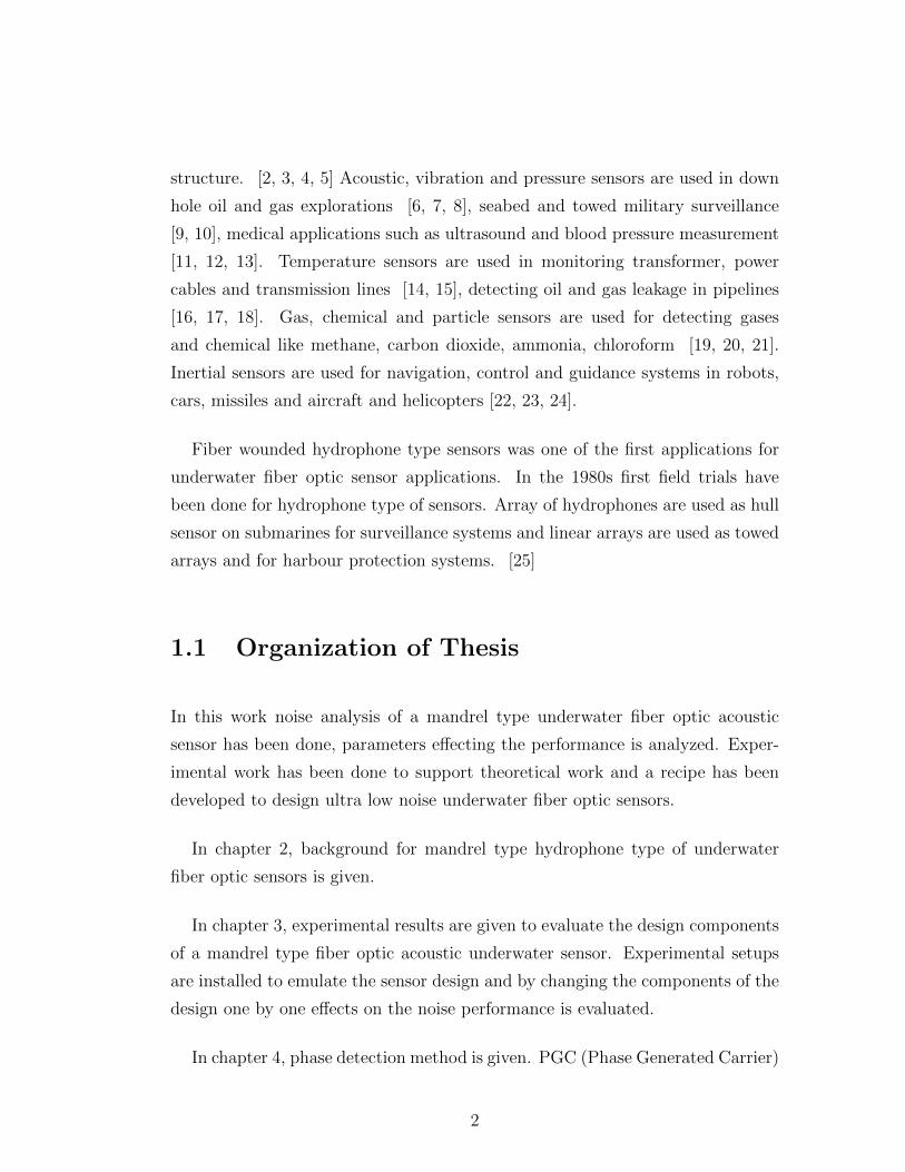
Figure 2.1: a) Frustrated total internal refraction b) Lateral misalignment c)Micro bending type of fiber optic acoustic sensors. Arrows shows fiber movementdirection due to perturbation

changes. Frustrated total internal refraction, lateral misalignment, micro bending

type of sensors can be given example for intensity based fiber optic acoustic sen-

sors. [29] Since the intensity based fiber optic sensors works on a loss mechanism,

they are limited with the minimum optical power that can be detected and in

order to have a very high sensitive sensor, very small optical powers have to be

detected, because of dynamic range and the sensitivity of the intensity based fiber

optic sensors are limited with the detector that is used and their performance is

not as good as the phase detection based fiber optic acoustic sensors.

Phase detection based fiber optic acoustic sensors detects acoustic signals by

5

strain generated by the pressure change on fiber optic cable. Strain on fiber

optic cable cause refractive index change and physical length change. As a result

optical path and phase of the light passing through the fiber changes. In this

work I will concentrate on phase detection based fiber optic acoustic sensors.

Fractional phase change in fiber optic sensors due to pressure change ∆P is given

as;

∆φ

φ∆P=

1

∆P

(εz −

n2eff

2[εr(p11 + p12) + εzp12]

)(2.1)

where εz and εr are axial and radial component of strain, p11 and p12 are the

Pockel’s coefficients, φ=neffkL is the total phase, k = 2πλ

, λ is the wavelength and

L is the fiber length. First term in the equation represents the contribution from

the length change of the fiber and the second term represents the contribution

coming from the refractive index change caused by the elastooptic effect. [30]

Figure 2.2: Drum shaped fiber optic acoustic sensor

In order to amplify the responsivity of the sensor there are two common ap-

proaches. First one is to amplify the strain by a mechanical encapsulation on

the sensing fiber. Drum like structures are used to amplify the strain on sensing

fiber. One end of the drum is fixed and the other has a flexible membrane and

6

the sensing fiber passes through the drum. As the pressure change on the drum,

membrane moves back and forth pulling the sensing fiber and exerting strain on

sensing fiber. There is a trade of in this type of sensors, using large membrane

to increase responsivity of the sensor, decreases the mechanical resonance of the

flexible membrane to very low frequencies. At frequencies higher than the reso-

nance frequency responsivity of the sensor drops dramatically. Hence it is difficult

to have wide bandwidth high sensitivity sensors with drum configuration.

Figure 2.3: Mandrel Type Fiber Optic Acoustic Sensor

Other approach to increase the responsivity of the fiber optic acoustic sensor is

to increase the length of sensing fiber. Mandrel type of sensors are good example

of this approach. Sensing fiber is wound on a solid mandrel. As the pressure on

the mandrel changes, mandrel does the breathing motion and radially extends and

contracts. Breathing motion exerts strain on sensing fiber. As the length of the

fiber wound on mandrel increases responsivity of the sensor increases, but you can

not increase radius and length of the mandrel to increase the fiber winding area,

this will decrease the mechanical resonance. Size of the mandrel is limited by the

detection bandwidth. Resonance frequency should be higher than the maximum

detection frequency. Winding fiber more than one layer is one way to increase

fiber length but, as the fiber layer on the mandrel increases, mandrel becomes

7

more stiff and breathing motion is restricted. As a result the responsivity of the

sensor decreases.

Figure 2.4: a) Airbacked Mandrel Type b) Cross section of the mandrel

Mechanical design of the sensor and Young’s modulus of the material deter-

mines the resonance frequency of the mandrel and deflection of the mandrel

against the pressure change, therefore the responsivity of the fiber optic sen-

sor. Youngs modulus defines the elasticity of the material, therefore having a low

Young modulus results high sensitivity. Putting a concentric hole inside the man-

drel increases the deflection against the pressure change but in return robustness

of the sensor decreases and under deep water conditions because of the high static

pressure mandrel may get structurally damaged and collapse. Without compro-

mising the robustness of the sensor, a foaming layer with low Young modulus

is used over a stiff mandrel and the responsivity is increased with the flexibility

of the foaming layer and the integrity of the of the sensor is ensured with the

stiff mandrel. Sensing fiber wound on the mandrel has to be protected from the

corrosion of the sea water, for that purpose a whole sensor should molded with

a thin polymer layer which is compliant with the sensor and should not decrease

the sensitivity of the fiber optic sensor. Design of the sensor mandrel is composed

of first selecting mandrel, foaming and molding layer materials and then deter-

mining the mechanical dimensions such as length of the mandrel, inner and outer

diameter of the mandrel which specifies the resonance frequency of the sensor. By

optimizing the design parameters maximum deflection of the mandrel structure

8

against pressure change is obtained for a specific detection bandwidth. Breathing

motion of the mandrel stretches the sensing fiber wound on the mandrel resulting

phase change of the laser passing through the fiber. Responsivity of the fiber

optic acoustic sensors are generally defined in dB re 1 rad/µPa unit and by in-

creasing the responsivity of the sensor, higher phase change will be obtained for

the same pressure change. [31, 32]

Figure 2.5: Mach- Zender interferometer configuration

Phase change in laser passing through the fiber can not be detected directly

since photodetectors with 1014 Hz bandwidth does not exist. In order to detect

the phase change caused by the acoustic signal an interferometer with the same

length reference arm is used to convert phase change to intensity modulation.

One arm of the interferometer is isolated from the acoustic signal and mixed with

the sensing arm and phase difference between the reference and the sensing arms

converted into intensity modulation by the interferometer. Michelson and Mach-

Zender interferemeters commonly used. Michelson interferometer uses one cou-

pler which divides the laser source in two arms, sensor and reference arms. Laser

passing through the sensor and reference arms reflected from the mirrors and

transverse the same path than mixed at the coupler and directed to the detector.

Same coupler is used for both dividing and recombining the laser. Mach-Zender

interferemoter uses two couplers one for dividing the signal and the second coupler

is used for combining the lasers coming through the sensor and reference arms.

9

Figure 2.6: Michelson interferometer configuration

Combined signals directed to detectors. Laser transverse in forward direction

in Mach-Zender interferometer, whereas in Michelson interferometer laser trans-

verse in both forward and backward directions. Michelson interferometers looks

like the folded version of Mach-Zender interferometer and in terms of optical loss

budget they are similar, however there are differences. Michelson interferometer

uses one coupler less than the Mach-Zender interferometer and it is physically

easier to package. Due to the fact that laser passes twice from both reference and

sensor arms optical phase shift due to the acoustic signal is doubled. Michelson

interferometer configuration depends on the reflection mechanism, therefore it is

sensitive to other reflections such as Rayleigh scattering induced back reflections

and forms unintended interference which significantly contributes to noise of the

system. On the other hand Mach-Zender interferometer has more components

and lower responsivity compared to Michelson interferometer, but it is immune to

scattering mechanisms in terms of noise performance since laser transverse only

in forward direction in Mach-Zender interferometer configuration.

Performance of a sensor can be evaluated in terms of responsivity, noise perfor-

mance and dynamic range. Responsivity of the phase detection based underwater

10

acoustic sensors determined by the optomechanical design of the sensor head as

given above. Dynamic range of a sensor is determined by the minimum and max-

imum acoustic signal levels that can be detected. Minimum detectable pressure

level is determined by both responsivity and the noise performance of the sensor.

MinimumDetectablePressure(µPa/

√Hz

)=SystemNoiseLevel

(rad/√Hz

)Responsivity (rad/µPa)

(2.2)

2.2 Noise Performance of Interferometric Fiber

Optic Acoustic Sensors

In this work, noise performance of an interferometric fiber optic acoustic sensor

will be analyzed, this type of sensors are composed of an interferometer, laser

source, photodetectors and sensor probe. Effects of the parameters such as phase

noise of the laser source, relative intensity noise of the laser source, interferometer

imbalance, and detector noise will be analyzed in the preceding sections.

2.2.1 Interferometer Imbalance

Monochromatic light can be modeled as a scalar wave ψ(r, t) where it is a function

of time, t and spatial position r. Electric field and magnetic field components of

light satisfies the following scalar wave equation derived from Maxwell’s equa-

tions.

52ψ (r, t) =1

c2δ2ψ (r, t)

δt2(2.3)

where 52 is the Laplacian operator and c is the speed of light. Any function

that satisfies the above equation can represent optical waves. Light propagating

11

through a single mode fiber can be modeled as a monochromatic plane wave for

the sake of simplicity and it is mathematically represented as,

ψ (~r, t) = E0exp(i(~k.~r − 2πυt

))(2.4)

where E0 is the amplitude of the field, ~k is the propagation wave vector and υ

is the frequency of the light. Assume planar wave is propagating in z direction,

wave function simplifies and becomes E0exp (i (kz − wt)) where w = 2πυ is the

angular frequency of the light. [33]

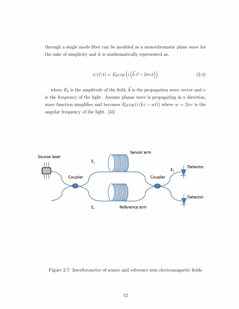
Figure 2.7: Interferometer of sensor and reference arm electromagnetic fields

12

Interference of light propagating through the reference arm and sensor arm

can be given as;

Et = Esexp (i (kLs − wt+ φs)) + Erexp (i (kLr − wt+ φr)) (2.5)

where Es, Er are the amplitude of the electromagnetic field in sensor arm and

reference arm, Ls and Lr are the length of sensor arm and reference arm of the

interferometer and φs and φr are the phase changes of sensor and reference arms.

Photodetectors can only detect the intensity of light since the frequency of the

light is very high. The intensity of the light is proportional to time averaged

value of the squared electric field. Iα〈E.E∗〉. Intensity of the light detected at

the detector can be calculated as below.

IT = 〈(Es + Er) . (Es + Er) ∗〉 =| Es |2 + | Er |2 +2Re (EsE∗r ) (2.6)

=| Es |2 + | Er |2 +2 | Es || Er | cos (φs − φr + k (Ls − Lr)) (2.7)

The light intensity at the output of the interferometer is not addition of inten-

sities coming from sensing arm and reference arms. Reference arm of the fiber

optic sensor is used to balance the interferometer and isolated from the acoustic

signal, therefore we assume that φr=0, there is no phase change due to acoustic

signals in reference arm. The intensity at the output of the interferometer is given

as,

IT = Is + Ir + 2√IsIrcos (φs + k (∆L)) (2.8)

where ∆L is the difference of the sensing arm length and the reference arm

length. As it can be seen from the above expression path imbalance has role in the

interferometer output. When we look at the expression above, path imbalance

term is added to the phase signal coming from sensing arm of the interferometer.

Therefore, we can interpret that path imbalance directly effects the phase noise

of the interferometric fiber optic acoustic sensor.

13

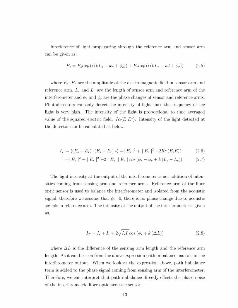
2.2.2 Laser Source Phase Noise

Although the laser sources are known as single frequency light sources, they do

have certain linewidth (lw) which results the corruption of phase coherence of the

photons leaving the laser after propagating a certain distance. The distance in

which the phase coherence is substantially preserved is defined as the coherence

length. Coherence length is calculated as,

Lcoherence = cτcoherence =c

πlw(2.9)

where c is the speed of light and τcoherence coherence time. Depending on the

linewidth of the laser coherence length can change dramatically.

Figure 2.8: Coherence of laser after propagating coherence length

Laser phase noise is due to the fluctuations of optical phase. As it can be seen

from the coherence schematic above, linewidth of the laser is one of the reason

for phase noise. Linewidth and the laser phase noise used as if they represent

the same thing, but in reality linewidth of the laser is determined by the low

frequency component of the phase noise. In many cases linewidth is given as the

phase noise of the laser, but in some applications complete phase noise spectrum

of the laser is used. [34] In two beam interferometers noise power at the output of

14

the interferometer is proportional to the coherence time of the laser source. [35]

Therefore noise of an interferometric fiber optic sensor is directly effected from

the linewidth of the laser source, or phase noise of the laser source.

2.2.3 Laser Source Relative Intensity Noise

Relative intensity noise(RIN) is the term defining the intensity flactuations of

the laser source. It is defined as variation of the power normalized to the average

power. The optical power of a laser source can be define as;

P (t) = P + δPRIN =δP

P(2.10)

RIN =δP

P(2.11)

average power and a zero mean δP fluctuating around the average power.

Statistical description of the relative intensity noise is defined as the Fourier

transform of the aotucorrelation of the intensity noise which gives a power spectral

density as a function of frequency.

S (f) =2

P 2

∫ ∞−∞〈δP (t) δP (t+ τ)〉 exp (i2πfτ)dτ (2.12)

The units of power spectral density of the RIN is in Hz−1, generally it is also

given in logarithmic units as dBc/Hz. Datasheets of the commercial products

commonly gives root mean square RIN parameter which is the square root of the

power spectral density integrated over an interval of [f1,f2].

RIN rms =δP

P rms=

√∫ f2

f1S (f) df (2.13)

In fiber optic sensing, interferometers are used to convert phase change to

intensity modulation. Phase change is demodulated from the intensity by using

15

different methods. Laser intensity noise adds noise to intensity modulation at the

output of the interferometer and spoils the demodulated phase term. Therefore,

having a lower laser intensity noise will improve the noise performance of a fiber

optic interferometric sensor.

2.2.4 Detector Noise

Photodetector noise is composed of shot noise, dark current and thermal noise

but commercial products gives noise equivalent power (NEP) parameter to rep-

resent the noise of the photodetectors. When there is no light illuminated on

the detector, the optical power value that makes SNR one is defined as the NEP

parameter. NEP parameter is calculated as,

NEP =inoiseR

(2.14)

where, inoise is the spectral current noise at the output of the detector when

there is no light illuminated and R is the responsivity of the photodetector. The

unit of NEP is given as W/√Hz.

Photodetector is used to convert optical signal to electrical signal. During this

conversion, detector noise is added to electrical signal representing the output of

the interferometers. This electrical signal is used to demodulate the phase change

caused by the sensing unit of the fiber optic acoustic sensor. Therefore, choosing

a detector with lower NEP value will improve the noise performance of the fiber

optic acoustic sensor.

16

Chapter 3

Optical Noise Characterization

In this chapter, experimental setups will be constructed to compare the effects

of the design parameters on the noise performance of the fiber optic acoustic

sensors. For this purpose complete sensor system will not be constructed but

similar experimental systems will be constructed emulate the sensor system and

effects of the design parameters will be analyzed.

3.1 Interferometer Imbalance

Interferometer imbalance is one of the parameters that is effecting the noise of

an interferometric fiber optic acoustic sensor. In order to analyze effect of the

interferometer imbalance the below experimental setup is constructed. As the

laser source PS-NLL model numbered product of Teraxion is used. It is a narrow

linewidth (≤ 5kHz) laser source with center wavelength at 1550nm. At the out-

put of the laser source an isolator is used to block the back reflections that can

spoil the stability of the laser. VOA (variable optical attenuator) is used to adjust

the power level for preventing detector saturation. Mach-Zender type interferom-

eter is used, and two 50/50 coupler is used to construct the interferometer. First

coupler is used to divide laser source in two arms and the second coupler is used

17

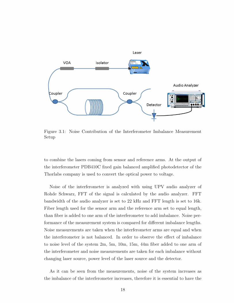
Figure 3.1: Noise Contribution of the Interferometer Imbalance MeasurementSetup

to combine the lasers coming from sensor and reference arms. At the output of

the interferometer PDB410C fixed gain balanced amplified photodetector of the

Thorlabs company is used to convert the optical power to voltage.

Noise of the interferometer is analyzed with using UPV audio analyzer of

Rohde Schwarz, FFT of the signal is calculated by the audio analyzer. FFT

bandwidth of the audio analyzer is set to 22 kHz and FFT length is set to 16k.

Fiber length used for the sensor arm and the reference arm set to equal length,

than fiber is added to one arm of the interferometer to add imbalance. Noise per-

formance of the measurement system is compared for different imbalance lengths.

Noise measurements are taken when the interferometer arms are equal and when

the interferometer is not balanced. In order to observe the effect of imbalance

to noise level of the system 2m, 5m, 10m, 15m, 44m fiber added to one arm of

the interferometer and noise measurements are taken for each imbalance without

changing laser source, power level of the laser source and the detector.

As it can be seen from the measurements, noise of the system increases as

the imbalance of the interferometer increases, therefore it is essential to have the

18

Figure 3.2: Noise Contribution of the Interferometer Imbalance

imbalance of the interferometer as small as possible. For this purpose a reference

mandrel is used to balance the interferometer and same length of fiber is wound

over the reference mandrel. Responsivity of a mandrel type fiber optic acoustic

sensor is increased by increasing the fiber length wound over the sensing mandrel.

Assuming 44m fiber is used for the sensing mandrel, if a reference mandrel is not

used to balance noise floor of the sensor system increases from 10−6V/√Hz to

10−4V/√Hz meaning 40dB increase in the noise floor.

3.2 Laser Source

Laser source used in the fiber optic acoustic sensor is effecting the noise per-

formance of the sensor system because of the phase noise and RIN of the laser.

Since it is impossible to tune phase noise and RIN parameters of a laser, I have

used three different laser sources to see the effect on the noise floor of the sys-

tem. First one is PSL-450 from Princeton Lightwave company, which has the

19

Figure 3.3: Noise Contribution of the Laser Source

worst linewidth value 12nm corresponding to approximately 1.5THz. Second

laser source is the EM4 high power DFB laser of the Gooch&Housego company

which has low RIN value (-150dBc/Hz ) and 1Mhz linewidth. Third laser source

is Pure Spectrum-Narrow Linewidth Laser (PS-NLL) of the Teraxion company

which has very narrow linewidth, 5kHz, and RIN value of this laser is -130dBc/Hz.

Parameters of the lasers can be seen at the table.

Table 3.1: Laser Source ParametersPSL 450 EM4 DFB Laser Teraxion PS-NLL

RIN - -150dBc/Hz -130dBc/HzLinewidth 1.5 THz 1Mhz 5kHz

Measurements are taken with balanced Mach-Zender interferometer and for

each laser source and power levels are set to the same level at the output of the

interferometer by using variable optical attenuator. At the output of the inter-

ferometer PDB410C fixed gain balanced amplified photodetector of the Thorlabs

company is used and noise of the setup is measured with UPV audio analyzer. As

20

it can be seen from the Figure 3.3 quality of the laser source is effecting the sys-

tem noise performance. Worst noise measurement is taken with PSL- 450 laser.

This laser has 12nm linewidth and RIN parameter is not given for this laser.

Best noise performance is taken with low linewidth PS-NLL laser, which has the

lowest linewidth value. It is obvious that the laser source is effecting the noise

performance of fiber optic acoustic sensors. It can be interpreted that having a

lower linewidth laser source results lower noise floor, but it is difficult to interpret

the effect of the RIN of the laser source on the noise performance of the sensor

system. In order to analyze the effect of RIN on the noise performance of fiber

optic acoustic sensors, measurement with different laser sources having similar

linewidth and different RIN values should be taken. What we have learned from

these measurements is that laser source with low linewidth should be used to get

low noise performance underwater fiber optic acoustic sensors.

3.3 Photodetector

Photodetector used in the fiber optic acoustic sensor is the part where the laser

intensity is converted into electrical signals, since the bandwidth of the current

detector technology is not enough to catch the phase change, interferometers are

used to convert the phase change into intensity modulation. Commercial detec-

tors have NEP (noise equivalent power) value in their datasheet to represent the

noise performance and responsivity values to conversion gain from light intensity

to voltage.

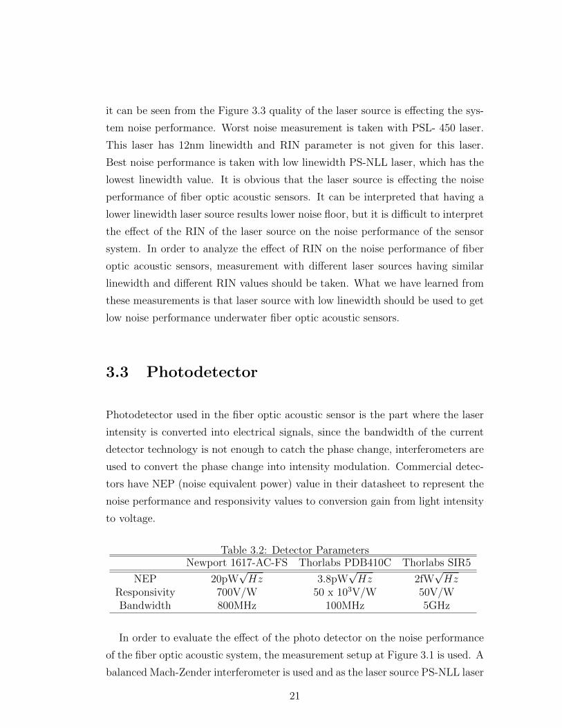
Table 3.2: Detector ParametersNewport 1617-AC-FS Thorlabs PDB410C Thorlabs SIR5

NEP 20pW√Hz 3.8pW

√Hz 2fW

√Hz

Responsivity 700V/W 50 x 103V/W 50V/WBandwidth 800MHz 100MHz 5GHz

In order to evaluate the effect of the photo detector on the noise performance

of the fiber optic acoustic system, the measurement setup at Figure 3.1 is used. A

balanced Mach-Zender interferometer is used and as the laser source PS-NLL laser

21

of the Teraxion company is used. Noise of the system is measured with UPV audio

analyzer of the Rohde&Schwarz company and FFT parameters are the same as

before. Three different photodetectors are used and noise measurements are taken

for each detector. First detector is the balanced InGaAs PIN detector with fixed

gain, Newport 1617-AC-FS, of Newport company, which has 800MHz bandwidth,

700V/W responsivity and 20pW√Hz NEP. Second detector is the PDB410C

of the Thorlabs company. This detector is an amplified InGaAs PIN detector

with 100MHz bandwidth, 50 x 103V/W responsivity and 3.8pW√Hz NEP. Third

detector is SIR5 InGaAs PIN detector of the Thorlabs company, which has 5GHz

bandwidth, 50V/W responsivity and 2fW√Hz NEP. This detector does not have

an amplifier but 50 ohm termination and it is powered from a battery.

Figure 3.4: Noise Contribution of Detector

Measurement results shows that the NEP value of the detector is determining

the noise floor of the fiber optic acoustic sensor, with the same measurement setup

lower NEP parameter results lower noise floor. One has to notice that NEP value

is given as noise spectral density, NEP value is multiplied with the square root

of the bandwidth to calculate noise of the detector. Using higher bandwidth

than the required bandwidth results extra noise. When we look at the noise

22

measurements SIR5 has the lowest noise floor, however it is not an amplified

detector and responsivity of the detector is lower than the other detectors. Since

the responsivity is lower, more optical power is needed to obtain the same voltage

level. Noise level obtained with SIR5 detector is quite low, it can be detected

with an audio analyzer, but with a standard electronic circuit you should either

add an amplifier circuit to increase the voltage level which will add extra noise,

or optical power should be increased.

In order to have the optimum performance for a fiber optic acoustic sensor

system, detector with minimum NEP value and maximum responsivity should

be used and the bandwidth of the detector shouldn’t be more than the required

bandwidth.

3.4 Interferometer Type

One main part of the fiber optic acoustic sensor is the interferometer that is used

to convert phase change of the laser in to intensity modulation. Mach-Zender and

Michelson interferometers are two common interferometer types that are used in

the fiber optic acoustic sensor design.

Figure 3.5: Mach-Zender interferometer noise measurement setup

23

Figure 3.6: Michelson interferometer noise measurement setup

Schematic figures for Michelson and Mach-Zender noise measurement setups

are seen above. In both measurement setups, PS-NLL laser source of the Teraxion

company is used and PDB410C fixed gain balanced amplified photodetector of

Thorlabs is used as the detector. Noise measurements are taken with UPV audio

analyzer of the Rohde&Schwarz, and FFT bandwidth is set to 22kHz and FFT

length is set to 16k for both noise measurements. For both interferometer systems

power levels reaching to the detector is adjusted to the same level.

Michelson interferometer seems like the folded version of the Mach-Zender

interferometer, the laser on the both sensor and reference arms are reflected back

and mixed with same coupler that divides the laser in two arms. Because of this,

laser travels the same path twice and physical length of the imbalance is multiplied

by two for Michelson interferometer. Therefore, adding 1m of fiber length to

one arm results 2m imbalance at the interferometer. Michelson interferometer

depends on the reflection of the laser in both arms, therefore it is sensitive to

other reflections such as impurity, Rayleigh induced back scattering and these

reflections become extra noise sources for the system.

Mach-Zender interferometer has forward laser propagation, hence it is more

24

Figure 3.7: Noise Contribution of the Interferometer Type

immune to Rayleigh scattering type of noise sources. But on the other hand,

Mach-Zender interferometer has more components and since laser pass through

the sensor arms once it has half the sensitivity compared to Michelson interfer-

ometer.

Looking at the noise measurements of Mach-Zender and Michelson interfer-

ometer setups , we observe similar noise floor levels except the lower frequencies.

Michelson interferometer has higher noise level at lower frequencies and this might

be the result of the sensitivity of the Michelson interferometer to scattering mech-

anisms. It can be claimed that Mach-Zender interferometer is more robust than

the Michelson interferometer in terms of the noise performance.

25

Chapter 4

Phase Detection Methods

Interferometric fiber optic detectors are evaluated by measuring phase difference

between a reference and sensor arms. Intensities at the output of the interferom-

eter changes with respect to phase difference ( δφ = φs − φr ). Intensity at the

output of the interferometer is given as,

I1 = Is + Ir + 2√IsIrcos (δφ) (4.1)

I2 = Is + Ir − 2√IsIrcos (δφ) (4.2)

where Ir and the Is are the intensities at the reference and sensor arm of the

interferometer. A more general representation is given as,

I1,2 = I0 (1± V cos (δφ)) (4.3)

where I0 = Ir + Is is the average power of the laser source, V is the visibility

of the interferometer which is defined as 2√IsIr/ (Ir + Is). Output of the inter-

ferometer is nonlinearly changes with the phase difference between the arms of

26

the interferometer, cosine term represents the nonlinear relation of phase change

to output of the interferometer. [36]

Figure 4.1: Interferometric output with phase bias φe and small signal phasechange δφ

Environmental effects have low frequency noise effect on the phase term which

can be represented as the phase bias point φe, this value drifts slowly with time

and phase bias point changes by slowly with time. Phase change coming from the

difference of the phases of reference and sensor arms can be represented as the

small signal phase change δφ. When the phase bias is at the odd multiples of π/2,

interferometer is at the quadrature point of phase bias and shows linear response

to small signal phase difference δφ. When the phase bias is at the multiple

values of π cosine term is at either maximum or minimum phase bias point and

interferometer exhibits nonlinear behaviour resulting distortion in small signal

phase changes.

Environmental effects changes slowly and phase bias moves away from quadra-

ture points to nonlinear points where small signal response is perturbated and

signal fading occurs.[37] One method to overcome the signal fading is to use active

27

control of phase bias point by adding a phase compensators to interferometer. [38]

Phase compensation is done either with a phase modulator or a piezoelectrically

stretched coiled fiber.

Figure 4.2: Phase compensation in Mach-Zender interferometer

Quadrature phase bias points are when both output of the interferometer

is equal. Outputs of the interferometer are I1 = I0 − V cos (δφ) and I1 =

I0 +V cos (δφ). Differential output of the interferometer is used as error term and

a closed loop feedback system is installed to keep the phase bias at the quadra-

ture point. Compensators at the interferometer actively corrects the phase bias

by adding phase to one arm of the interferometer. By using compensators low

frequency noise stemming from the environmental effects can be corrected and

nonlinear perturbation from the output of the interferometric sensor can be elim-

inated. Highest frequency noise signal that can be corrected is limited with the

bandwidth of the closed loop feedback. In order to have a successfull phase de-

tection with phase compensation method, noise frequency and the sensor signal

should be separate from each other.

28

Piezoelectrically stretched fiber coils and phase compensators are bulky and

heavier than the sensor itself. Another major disadvantage of compensator

method is multiplexing sensor arrays. Since this method is a closed loop sys-

tem tracking the error term and keeping the phase bias on the quadrature point,

when array of sensors are multiplexed compensators for each sensor element must

be used and the complexity of the control electronics is multiplied by the sensor

number.

4.1 Phase Generated Carrier Method

Phase Generated Carrier (PGC) method is a passive open loop technique. This

technique introduces a phase modulation outside the signal bandwidth. Mod-

ulation signal carries the signal of interest to sidebands and upconverts them,

therefore eliminates the low frequency noise. [39] Light intensity at the output of

the interferometer can be written as;

I0 = A+Bcos (θ (t)) (4.4)

where, A and B are the constants representing the average intensity and the

visibility of the interferometer and θ (t) is representing the time varying phase

difference between the arms of the interferometer. When a sinusoidal modula-

tion signal with a frequency ω0 and amplitude C is applied to one arm of the

interferometer, intensity at the output of the interferometer becomes,

I0 = A+Bcos (Csin (ω0t) + φ (t)) (4.5)

where the amplitude of the modulation signal C is defined as the modulation

depth and ω0 is the carrier frequency of the PGC method. Carrier signal is

generated with a phase modulator or piezoelectrically stretched fiber coil. The

signal of interest is represented with φ (t). If we expand intensity in terms of

29

Bessel functions we get,

I0 = A+B

((J0 (t) + 2

∞∑k=1

(−1)k J2k (C) cos (2kω0t)

)cos (φ (t))

)

−B((

2∞∑k=0

(−1)k J2k+1 (C) cos ((2k + 1)ω0t)

)sinφ (t)

)(4.6)

I0 = A+B ((J0(C) + 2J2(C)cos(2ω0t) + 2J4(C)cos(4ω0t) + ...) cos(φ(t)))

−B ((2J1(C)sin(ω0t) + 2J3(C)sin(3ω0t) + ...) sin(φ(t))) (4.7)

where Jn(C) terms are the Bessel functions of the first kind. Intensity of

the interferometer is multiplied with cos(ω0t) and cos(2ω0t) functions and first

and second harmonic of the carrier signal with its sidebands are downconverted.

Downconverted signals are lowpass filtered to eliminate higher harmonics and two

baseband signals are generated. [40]

L1 = KJ1(C)sin(φ(t)) (4.8)

L1 = KJ2(C)cos(φ(t)) (4.9)

where K is the constant coming from the intensity amplitude. If we set the

modulation depth to C = 2.63, then coefficients of cos(φ(t)) and sin(φ(t)) be-

comes equal. J1=J2 Phase term φ(t) can be found by calculating the arctangent

of ratio of the baseband signals when C = 2.63

φ(t) = tan−1(KJ1(C)sin(φ(t))

KJ2(C)cos(φ(t))

)= tan−1

(sin(φ(t))

cos(φ(t))

)(4.10)

Downconverted baseband signals give sine and cosine of the interested phase

30

signal. Ratio of the baseband signals equals to the tangent of the phase signal,

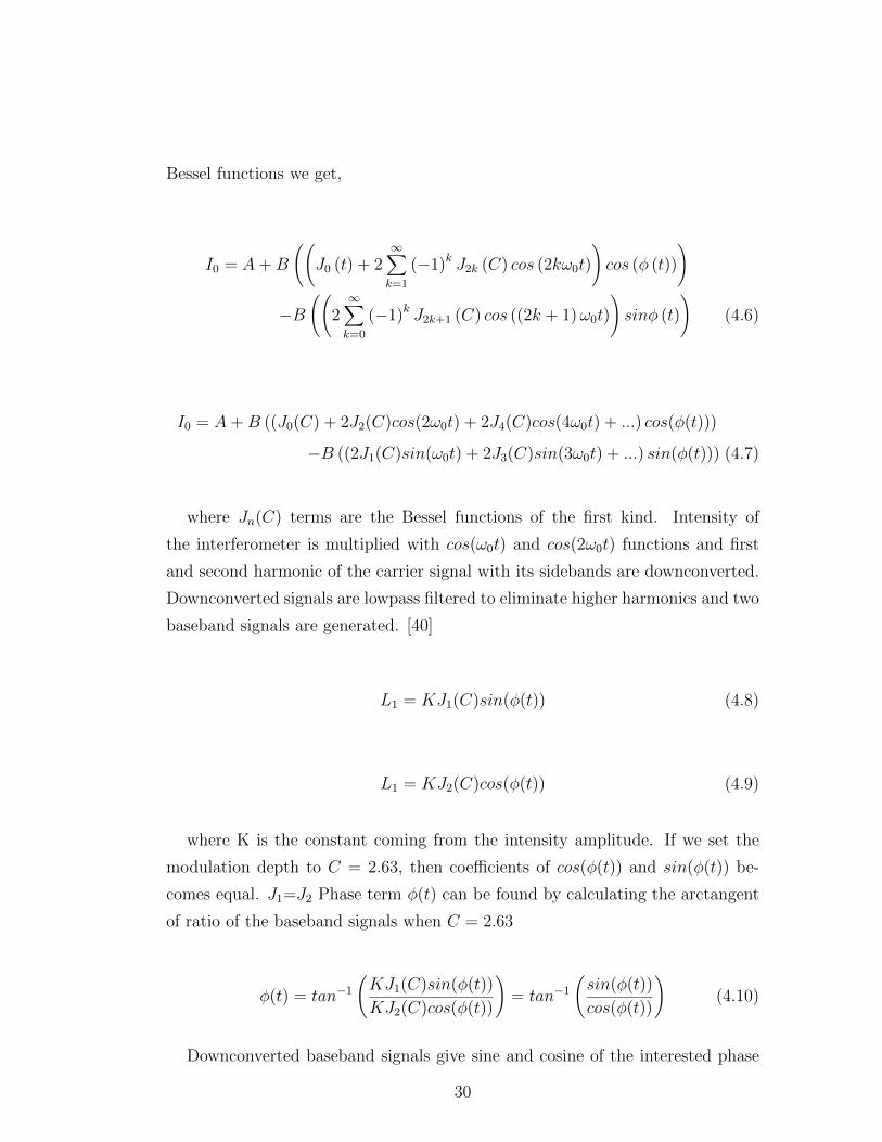
by calculating the arctangent value phase signal is obtained. [41]

Figure 4.3: Phase Generated Carrier- Arctangent Algorithm

Arctangent operation gives phase values between −π ≤ φ ≤ π. When phase

signal is larger than π or smaller than −π, it is wrapped over the unit circle

and phase value abrubtly jumps 2π, continuity of the signal is disturbed. Small

phase signals are demodulated without distrubting the signal shape, but for large

phase signals these abrubt jumps adds extra noise to the detected phase signal.

Therefore, dynamic range of the sensor becomes limited by one period of unit

circle, 2π.

In order to correct the large phase signals fringe counter is used. Signs of the

baseband signals, sin (φ) and cos (φ), are used to find the region of the phase sig-

nal and fringe count value is hold in the memory. When implementing the fringe

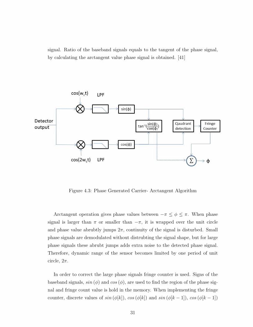
counter, discrete values of sin (φ[k]), cos (φ[k]) and sin (φ[k − 1]), cos (φ[k − 1])

31

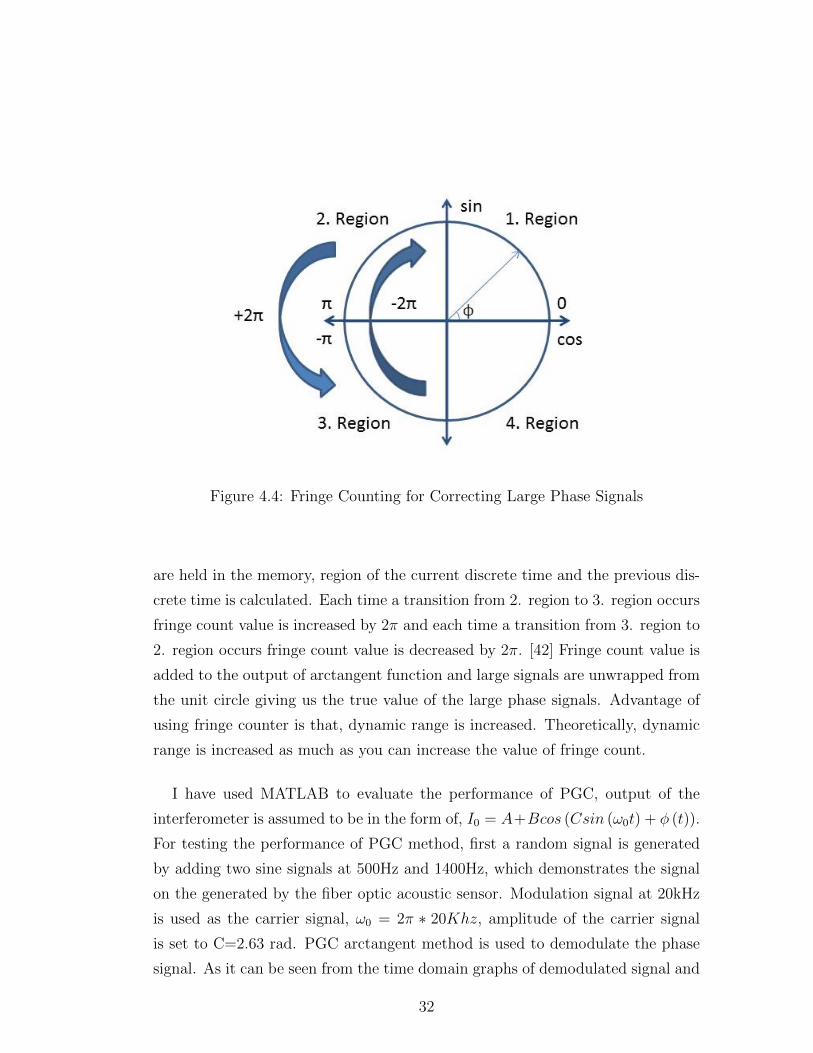
Figure 4.4: Fringe Counting for Correcting Large Phase Signals

are held in the memory, region of the current discrete time and the previous dis-

crete time is calculated. Each time a transition from 2. region to 3. region occurs

fringe count value is increased by 2π and each time a transition from 3. region to

2. region occurs fringe count value is decreased by 2π. [42] Fringe count value is

added to the output of arctangent function and large signals are unwrapped from

the unit circle giving us the true value of the large phase signals. Advantage of

using fringe counter is that, dynamic range is increased. Theoretically, dynamic

range is increased as much as you can increase the value of fringe count.

I have used MATLAB to evaluate the performance of PGC, output of the

interferometer is assumed to be in the form of, I0 = A+Bcos (Csin (ω0t) + φ (t)).

For testing the performance of PGC method, first a random signal is generated

by adding two sine signals at 500Hz and 1400Hz, which demonstrates the signal

on the generated by the fiber optic acoustic sensor. Modulation signal at 20kHz

is used as the carrier signal, ω0 = 2π ∗ 20Khz, amplitude of the carrier signal

is set to C=2.63 rad. PGC arctangent method is used to demodulate the phase

signal. As it can be seen from the time domain graphs of demodulated signal and

32

Figure 4.5: Random phase signal and demodulated phase signal with PGCmethod

the randomly generated signal, randomly generated signal can be demodulated

perfectly with PGC method.

There are few key point in PGC method that has to be taken carefully. Carrier

signal should be at least two time larger than the highest frequency of interest.

Since carrier signal and the second harmonic of the carrier signal is used to de-

modulate the phase signal. Acoustic signals are upconverted by the carrier signal

and its second harmonic signal. If the two times the highest frequency acoustic

signal has higher frequency than the carrier frequency, upconverted signals will

mix and demodulation will fail. Spectrum of the signal at the output of the

detector is shown schematically below.

33

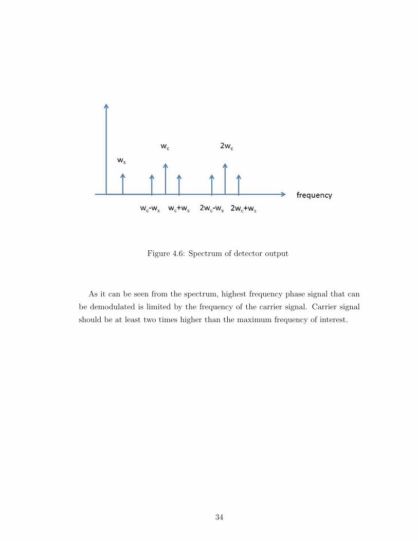
Figure 4.6: Spectrum of detector output

As it can be seen from the spectrum, highest frequency phase signal that can

be demodulated is limited by the frequency of the carrier signal. Carrier signal

should be at least two times higher than the maximum frequency of interest.

34

Chapter 5

Ultra Low Noise Fiber Optic

Acoustic Sensors for Underwater

Applications

Noise is a key parameter when evaluating the performance of an underwater

acoustic sensor. In order to detect an acoustic signal at the point of the sensor,

signal strength should be higher than the noise sources. For a passive underwater

acoustic sensor main noise sources can be defined as ambient noise, self noise of

the sensor and vessel noise. Self noise of the sensor is the noise source that is

stemming from the sensor itself. Ambient noise is the noise that is coming from

the sea and vessel noise is the noise source that occurs from the propellers and

propulsion machinery of the platform that is carrying the underwater acoustic

sensor. [43, 44] Since the noise source are not correlated with each other, total

RMS (root mean square) noise can be calculated by adding squares of the mean

noise sources than calculating the square root of the sum.

〈ntotal〉 =√〈nselfnoise〉2 + 〈nvesselnoise〉2 + 〈nambientnoise〉2 (5.1)

Passive underwater acoustics sensors are used for listening the acoustic signals

35

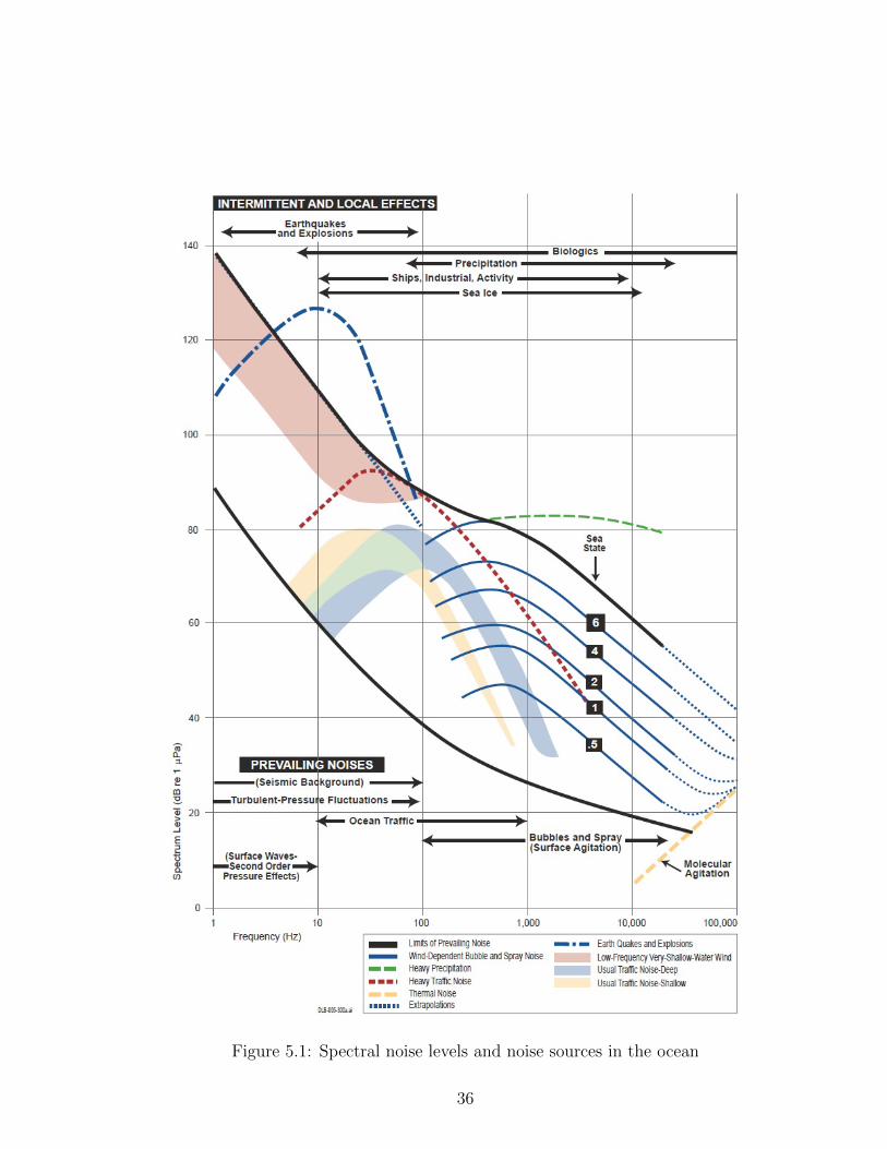
Figure 5.1: Spectral noise levels and noise sources in the ocean

36

generated by a target. Highest noise source is the one determining the noise level.

Self noise of the sensor can be improved by improving the design of the sensor.

In order to improve the performance of an underwater acoustic sensor, self noise

of the sensor should be lower than the ambient noise of the sea and vessel noise.

Spectral distribution of the ambient noise of the ocean and its sources are

shown in the figure. Noise in the ocean is present because of the effects coming

from the surface of the sea, seismic noise coming from the bottom of the sea, tur-

bulance and molecular motion inside sea and the living creatures in the sea. Noise

contribution from the seismic disturbances coming from the seabed contributes

to the low frequency spectrum of the ambient noise. [45]

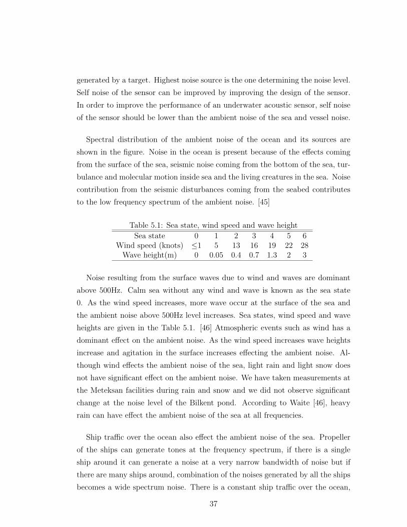
Table 5.1: Sea state, wind speed and wave height

Sea state 0 1 2 3 4 5 6Wind speed (knots) ≤1 5 13 16 19 22 28

Wave height(m) 0 0.05 0.4 0.7 1.3 2 3

Noise resulting from the surface waves due to wind and waves are dominant

above 500Hz. Calm sea without any wind and wave is known as the sea state

0. As the wind speed increases, more wave occur at the surface of the sea and

the ambient noise above 500Hz level increases. Sea states, wind speed and wave

heights are given in the Table 5.1. [46] Atmospheric events such as wind has a

dominant effect on the ambient noise. As the wind speed increases wave heights

increase and agitation in the surface increases effecting the ambient noise. Al-

though wind effects the ambient noise of the sea, light rain and light snow does

not have significant effect on the ambient noise. We have taken measurements at

the Meteksan facilities during rain and snow and we did not observe significant

change at the noise level of the Bilkent pond. According to Waite [46], heavy

rain can have effect the ambient noise of the sea at all frequencies.

Ship traffic over the ocean also effect the ambient noise of the sea. Propeller

of the ships can generate tones at the frequency spectrum, if there is a single

ship around it can generate a noise at a very narrow bandwidth of noise but if

there are many ships around, combination of the noises generated by all the ships

becomes a wide spectrum noise. There is a constant ship traffic over the ocean,

37

which has a contribution to ambient noise level of the sea. Even if there is no

ship traffic, no rain or wind or snow, no seismic disturbances, there will be still

ambient noise due to molecular motions of the ingredients of sea and the noise

due to fishes and plants living in the sea.

Evaluating an underwater acoustic sensor, self noise is good indication of per-

formance, if the self noise of the sensor is higher than the ambient noise, the

sensor noise will limit the minimum detectable pressure. If the self noise is better

than the ambient noise, minimum detectable pressure will be limited with the

ambient noise.

Velocity of an acoustic signal is determined by the properties of the propagation

medium such as density ρ and the elasticity modulus E. For fluids compressibility

χ is used to calculate the propagation speed of acoustic signal. Compressibility

χ is the inverse of elasticity modules E.

c =

√E

ρ=

√1

χρ(5.2)

In sea water propagation speed of acoustic signals is approximately c=

1500m/sec, but depending on the depth, pressure, salinity and temperature prop-

agation speed changes. Since the ocean is not an homogenous medium in terms of

salinity and temperature, propagation speed changes in the ocean. For example

after sunrise water in the sea starts to warm up from the surface and density of

the water changes from surface to down, which leads to a gradient of propagation

speed.

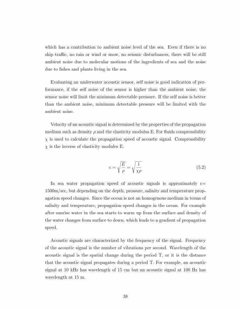
Acoustic signals are characterized by the frequency of the signal. Frequency

of the acoustic signal is the number of vibrations per second. Wavelength of the

acoustic signal is the spatial change during the period T, or it is the distance

that the acoustic signal propagates during a period T. For example, an acoustic

signal at 10 kHz has wavelength of 15 cm but an acoustic signal at 100 Hz has

wavelength at 15 m.

38

λ = cT =c

f(5.3)

Frequency of the acoustic signal also effects the attenuation of the signal, size

of the acoustic signal generators, target acoustic response. Frequency of the signal

determines the size of the wavelength, if the target is smaller than the wavelength

of the acoustic signal reflected energy gets smaller. Therefore, a specific target can

reflect more energy at smaller wavelengths. Acoustic signal generators becomes

larger as the frequency of the acoustic signal gets smaller.

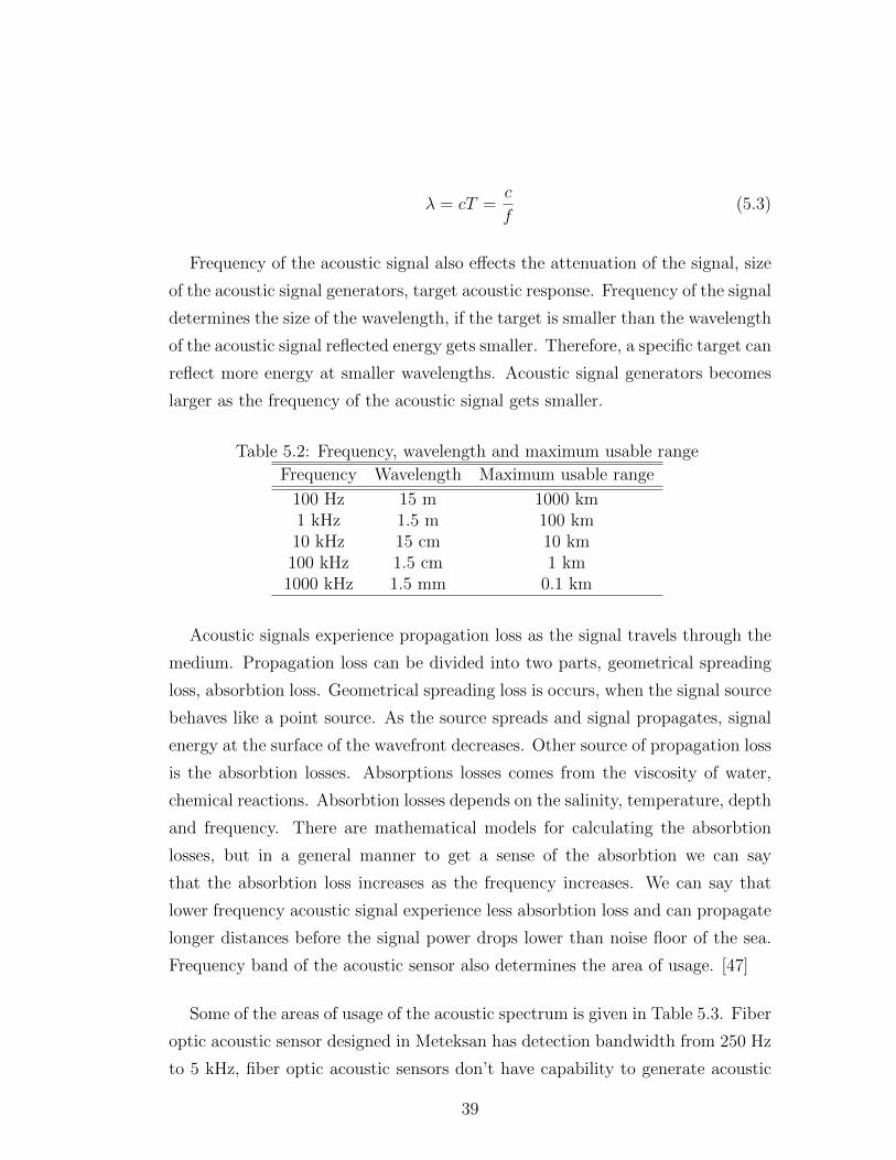
Table 5.2: Frequency, wavelength and maximum usable range

Frequency Wavelength Maximum usable range

100 Hz 15 m 1000 km1 kHz 1.5 m 100 km10 kHz 15 cm 10 km100 kHz 1.5 cm 1 km1000 kHz 1.5 mm 0.1 km

Acoustic signals experience propagation loss as the signal travels through the

medium. Propagation loss can be divided into two parts, geometrical spreading

loss, absorbtion loss. Geometrical spreading loss is occurs, when the signal source

behaves like a point source. As the source spreads and signal propagates, signal

energy at the surface of the wavefront decreases. Other source of propagation loss

is the absorbtion losses. Absorptions losses comes from the viscosity of water,

chemical reactions. Absorbtion losses depends on the salinity, temperature, depth

and frequency. There are mathematical models for calculating the absorbtion

losses, but in a general manner to get a sense of the absorbtion we can say

that the absorbtion loss increases as the frequency increases. We can say that

lower frequency acoustic signal experience less absorbtion loss and can propagate

longer distances before the signal power drops lower than noise floor of the sea.

Frequency band of the acoustic sensor also determines the area of usage. [47]

Some of the areas of usage of the acoustic spectrum is given in Table 5.3. Fiber

optic acoustic sensor designed in Meteksan has detection bandwidth from 250 Hz

to 5 kHz, fiber optic acoustic sensors don’t have capability to generate acoustic

39

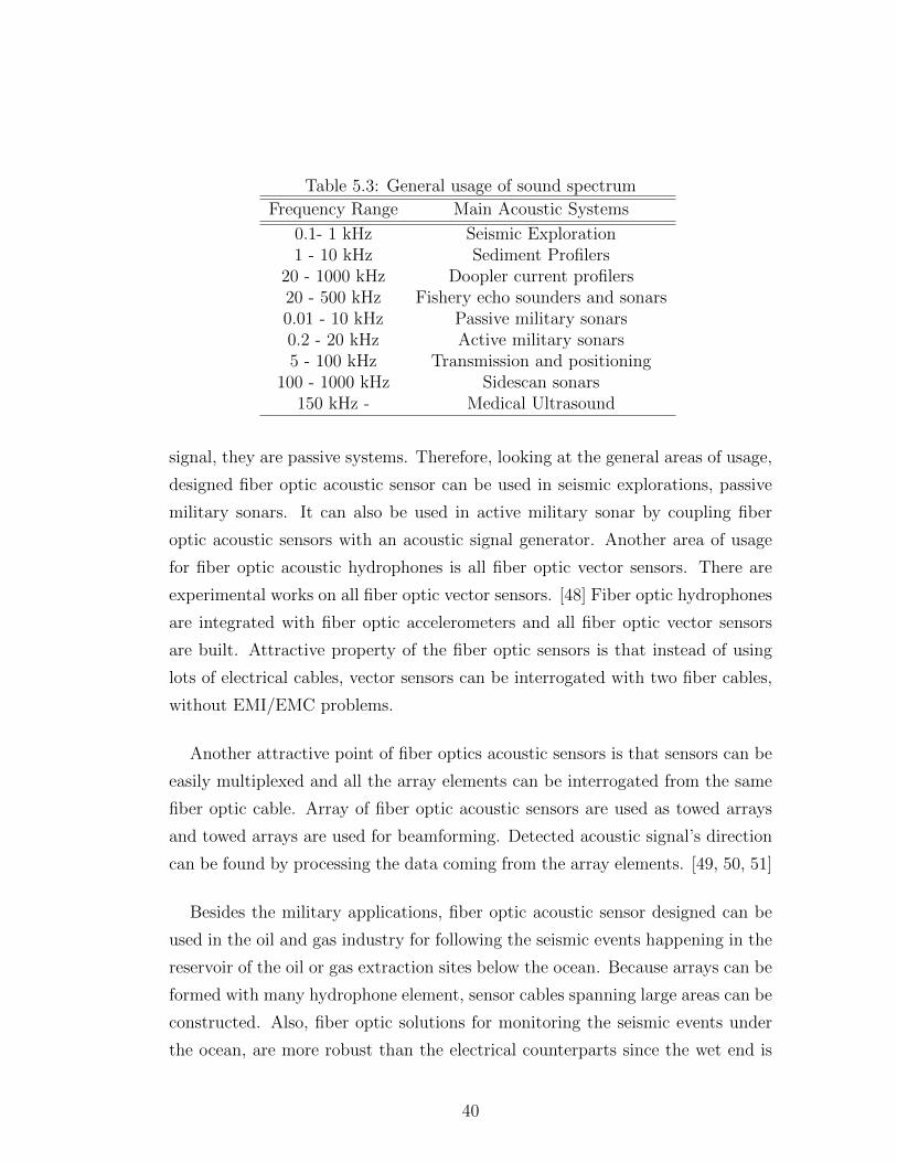
Table 5.3: General usage of sound spectrum

Frequency Range Main Acoustic Systems

0.1- 1 kHz Seismic Exploration1 - 10 kHz Sediment Profilers

20 - 1000 kHz Doopler current profilers20 - 500 kHz Fishery echo sounders and sonars0.01 - 10 kHz Passive military sonars0.2 - 20 kHz Active military sonars5 - 100 kHz Transmission and positioning

100 - 1000 kHz Sidescan sonars150 kHz - Medical Ultrasound

signal, they are passive systems. Therefore, looking at the general areas of usage,

designed fiber optic acoustic sensor can be used in seismic explorations, passive

military sonars. It can also be used in active military sonar by coupling fiber

optic acoustic sensors with an acoustic signal generator. Another area of usage

for fiber optic acoustic hydrophones is all fiber optic vector sensors. There are

experimental works on all fiber optic vector sensors. [48] Fiber optic hydrophones

are integrated with fiber optic accelerometers and all fiber optic vector sensors

are built. Attractive property of the fiber optic sensors is that instead of using

lots of electrical cables, vector sensors can be interrogated with two fiber cables,

without EMI/EMC problems.

Another attractive point of fiber optics acoustic sensors is that sensors can be

easily multiplexed and all the array elements can be interrogated from the same

fiber optic cable. Array of fiber optic acoustic sensors are used as towed arrays

and towed arrays are used for beamforming. Detected acoustic signal’s direction

can be found by processing the data coming from the array elements. [49, 50, 51]

Besides the military applications, fiber optic acoustic sensor designed can be

used in the oil and gas industry for following the seismic events happening in the

reservoir of the oil or gas extraction sites below the ocean. Because arrays can be

formed with many hydrophone element, sensor cables spanning large areas can be

constructed. Also, fiber optic solutions for monitoring the seismic events under

the ocean, are more robust than the electrical counterparts since the wet end is

40

in all fiber and the electrical parts such as interrogators, laser drivers are isolated

from water. There are successful examples of fiber optic acoustic sensors used in

reservoir monitoring.[52, 53, 54]

After evaluating the possible areas of usage for the fiber optic acoustic sensor

designed, performance of the sensor will be evaluated. First noise performance

of the fiber optic acoustic sensor will be evaluated. Noise measurement setup is

given below.

Figure 5.2: Noise Measurement Setup

Since the electronic card that will be used to interrogate the fiber optic acoustic

sensor is not completed, noise measurement are taken with OPD4000 optical

phase modulator of Optiphase company. OPD4000 uses phase generated carrier

method to demodulate the phase signal. Rest of the noise measurement setup

is used to emulate the fiber optic acoustic sensor system. Noise measurement

setup is designed as close as possible to the actual design of the sensor system to

reflect the real performance. Fiber optic part of the measurement setup is seen in

Figure 5.3. After laser input, an isolator is added to protect the laser source from

backreflections. Variable optical attenuator is used to adjust the power level used

41

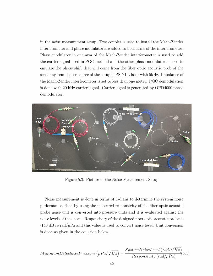
in the noise measurement setup. Two coupler is used to install the Mach-Zender

interferometer and phase modulator are added to both arms of the interferometer.

Phase modulator in one arm of the Mach-Zender interferometer is used to add

the carrier signal used in PGC method and the other phase modulator is used to

emulate the phase shift that will come from the fiber optic acoustic prob of the

sensor system. Laser source of the setup is PS-NLL laser with 5kHz. Imbalance of

the Mach-Zender interferometer is set to less than one meter. PGC demodulation

is done with 20 kHz carrier signal. Carrier signal is generated by OPD4000 phase

demodulator.

Figure 5.3: Picture of the Noise Measurement Setup

Noise measurement is done in terms of radians to determine the system noise

performance, than by using the measured responsivity of the fiber optic acoustic

probe noise unit is converted into pressure units and it is evaluated against the

noise levels of the ocean. Responsivity of the designed fiber optic acoustic probe is

-140 dB re rad/µPa and this value is used to convert noise level. Unit conversion

is done as given in the equation below.

MinimumDetectablePressure(µPa/

√Hz

)=SystemNoiseLevel

(rad/√Hz

)Responsivity (rad/µPa)

(5.4)

42

Figure 5.4: Noise Level of the Designed Fiber Optic Acoustics

Measured noise level is given in Figure 5.4. Measurement is done in the lab

environment, therefore there are peaks in the spectrum which comes from the

environment. Left axis of the measurement is the noise density in terms of radians

and right axis of the measurement is the noise density in terms of pressure. Noise

level above 100 Hz is close to 40 dB re µPa/√Hz which is close to sea state zero

of the ocean noise. Sea state zero is the state where there is no wind or wave and

no shipping traffic noise. It is almost impossible to find such state of the ocean.

Therefore, it is safe to say that noise level of the designed sensor is lower than

the ambient noise of the ocean. Contribution of the self noise of the fiber optic

acoustic sensor is negligible compared to the contribution of the ambient noise.

Acoustic signal detection by the designed fiber optic acoustic sensor is limited by

the ambient noise of the ocean. Improving the noise level further to lower levels

will not improve the performance of signal detection, because the ambient noise

is limiting the signal detection.

43

After measuring the noise level of the fiber optic acoustic sensor, phase change

with different amplitudes are applied at 1 kHz with the phase modulator which

emulates the fiber optic acoustic probe. By changing the amplitude of the phase

shift with phase modulator, demodulated phase amplitudes from the audio ana-

lyzer is recorded. In order to calculate the percentage linearity absolute value of

the percentage error is subtracted from 100. Percentage linearity is calculated as

below.

Linearity(%) = 100− Abs(ActualV alue−DetectedV alue) ∗ 100

ActualV alue(5.5)

Figure 5.5: Phase amplitude linearity

As the amplitude of the phase shift is changed, we observe from the measure-

ments that linearity of the sensor stays over 97 percents. Phase shift will occur

when the acoustic signal is detected by the fiber optic acoustic probe. As the

amplitude of the acoustic signal increases, detected signal stays linear.

Linearity of the fiber optic acoustic sensor in frequency is tested by changing

the frequency of the phase signal given from the phase modulator emulating

44

Figure 5.6: Phase amplitude linearity with frequency change

the fiber optic acoustic probe. Phase signal with amplitude 3.8 rad is applied

at different frequencies and percentage linearity of the detected phase signal is

calculated. Percentage linearity of the acoustic signal from 250 Hz to 3 kHz is

above 98 percent.

45

Chapter 6

Conclusion

Fiber optic sensor have many advantages over the counter technology sensors,

such as EMI immunity, low weight, flexible geometric design, no electrical con-

nection at the remote sensing point. Fiber optic sensor are being used in many

areas. Acoustic sensing, strain sensing, temperature sensing, magnetic field sens-

ing, rotation sensing, chemical/biomedical sensing are main areas where fiber

optic sensor are being used.

In this thesis, mandrel type fiber optic acoustic underwater sensors are an-

alyzed in terms of their noise performance. Experimental work and simulation

have been done to evaluate the design parameters of the mandrel type fiber optic

acoustic sensors.

In order to emulate fiber optic acoustic sensor experimental setups are con-

structed and experiments to analyze noise performance characteristics have been

done. Experiments have shown us that using a high quality laser source, which

has low phase noise and low RIN value, lowers the noise of the interferometer.

Experimental results also have shown us that imbalance of the interferometer

increases the noise level at the output of the interferometer. Interferometer type

used in the design of the mandrel type fiber optic sensor also effects the noise

at the output of the interferometer. Mach-Zender type interferometer have lower

46

noise level at lower frequencies compared to Michelson type of interferometers.

Photodetector used at the design of the fiber optic sensor also effects the noise

performance of the sensor. Lower NEP value detector gives lower noise floor

but responsivity of the photodetector is also important in terms of power budget

of the laser source. When using a lower responsivity photodetector laser power

should be increased in order to get meaningful voltage values at the output of

the detector. Therefore choosing a detector with a lower NEP value and higher

responsivity will be best solution for both noise performance of the sensor and

power budget of the laser source.

Performance of the fiber optic acoustic sensor is evaluated by it noise perfor-

mance, dynamic range and responsivity. Responsivity of the sensor is determined

by mechanical design of the mandrel, fiber length used on the sensor. Dynamic

range of the sensor is determined by the maximum and minimum acoustic signal

that can be detected. PGC method used to demodulate the phase change of the

interferometer has very large dynamic range because of fringe counting property.

Noise level of the fiber optic acoustic sensor should be compared with the envi-

ronmental noise of the medium it will be used. Ambient noise of the ocean is

effected by various effects. Noise levels are defined with sea states which defines

the noise level in different climatic conditions.

Noise level of the design is measured by using commercial product since the

electronic cards is not completed. While measuring the noise level an experi-

mental setup is installed to emulate the design. Low phase noise laser is used

with Mach-Zender interferometer, and the path imbalance of the interferometer

is set to less than one meter. Measured noise level about -100 dB rad/√Hz

above 100 Hz. Using the responsivity of the noise level measured in terms of

radians converted to pressure units. Responsivity of the designed sensor is -140

dB re rad/µPa, which gives noise level about 40 dB re µPa/√Hz noise level.

This noise level is equal to the noise level of the ocean at sea state zero (SS0).

Sea state zero is the level when there is no wind, wave or shipping traffic noise.

Therefore any signal above the ambient noise level of the ocean can be detected

with the designed fiber optic acoustic sensor. Noise level of the designed sensor

is lower than the ambient noise of the ocean, which means signal detection is

47

not limited with the sensor noise but it is limited with the ambient noise of the

ocean. Finally, linearity of the sensor against amplitude and frequency is tested

and measurement have shown the linearity is over 97 percent for both frequency

change and amplitude change.

48

Bibliography

[1] A. D. Kersey, “A review of recent developments in fiber optic sensor tech-

nology,” Optical Fiber Technology, vol. 2, no. 3, pp. 291 – 317, 1996.

[2] K. Kuang, R. Kenny, M. Whelan, W. Cantwell, and P. Chalker, “Embedded

fibre bragg grating sensors in advanced composite materials,” Composites

Science and Technology, vol. 61, no. 10, pp. 1379–1387, 2001.

[3] X. Pan, D. Liang, and D. Li, “Optical fiber sensor layer embedded in smart

composite material and structure,” Smart materials and structures, vol. 15,

no. 5, p. 1231, 2006.

[4] S. Melle, K. Liu, et al., “Wavelength demodulated bragg grating fiber optic

sensing systems for addressing smart structure critical issues,” Smart Mate-

rials and Structures, vol. 1, no. 1, p. 36, 1992.

[5] R. Maaskant, T. Alavie, R. Measures, G. Tadros, S. Rizkalla, and A. Guha-

Thakurta, “Fiber-optic bragg grating sensors for bridge monitoring,” Cement

and Concrete Composites, vol. 19, no. 1, pp. 21–33, 1997.

[6] A. D. Kersey, “Optical fiber sensors for permanent downwell monitoring

applications in the oil and gas industry,” IEICE transactions on electronics,

vol. 83, no. 3, pp. 400–404, 2000.

[7] G. Shiach, A. Nolan, S. McAvoy, D. McStay, C. Prel, and M. Smith, “Ad-

vanced feed-through systems for in-well optical fibre sensing,” in Journal of

Physics: Conference Series, vol. 76, p. 012066, IOP Publishing, 2007.

49

[8] T. Yamate, “Fiber optic sensors for the exploration of oil and gas,” in 19th

International Conference on Optical Fibre Sensors, pp. 700438–700438, In-

ternational Society for Optics and Photonics, 2008.

[9] J. Dakin, C. Wade, and M. Henning, “Novel optical fibre hydrophone array

using a single laser source and detector,” Electronics Letters, vol. 20, no. 1,

pp. 53–54, 1984.

[10] S. Goodman, S. Foster, J. Van Velzen, and H. Mendis, “Field demonstration

of a dfb fibre laser hydrophone seabed array in jervis bay, australia,” in

20th International Conference on Optical Fibre Sensors, pp. 75034L–75034L,

International Society for Optics and Photonics, 2009.

[11] D. Tosi, M. Olivero, and G. Perrone, “Low-cost fiber bragg grating vibroa-

coustic sensor for voice and heartbeat detection,” Applied optics, vol. 47,

no. 28, pp. 5123–5129, 2008.

[12] J. Dorighi, S. Krishnaswamy, and J. D. Achenbach, “Response of an embed-

ded fiber optic ultrasound sensor,” The Journal of the Acoustical Society of

America, vol. 101, no. 1, pp. 257–263, 1997.

[13] P. Morris, P. Beard, and A. Hurrell, “Development of a 50 mhz optical fibre

hydrophone for the characterisation of medical ultrasound fields,” in Proc.

IEEE Ultrasonics Symp, vol. 9, pp. 1747–1750, 2005.

[14] J. Deng, H. Xiao, W. Huo, M. Luo, R. May, A. Wang, and Y. Liu, “Optical

fiber sensor-based detection of partial discharges in power transformers,”

Optics & Laser Technology, vol. 33, no. 5, pp. 305–311, 2001.

[15] G. Yilmaz and S. E. Karlik, “A distributed optical fiber sensor for tempera-

ture detection in power cables,” Sensors and Actuators A: Physical, vol. 125,

no. 2, pp. 148–155, 2006.

[16] M. Nikles, B. H. Vogel, F. Briffod, S. Grosswig, F. Sauser, S. Luebbecke,

A. Bals, and T. Pfeiffer, “Leakage detection using fiber optics distributed

temperature monitoring,” in Smart Structures and Materials, pp. 18–25,

International Society for Optics and Photonics, 2004.

50

[17] B. Vogel, C. Cassens, A. Graupner, and A. Trostel, “Leakage detection sys-

tems by using distributed fiber optical temperature measurement,” in SPIE’s

8th Annual International Symposium on Smart Structures and Materials,

pp. 23–34, International Society for Optics and Photonics, 2001.

[18] D. Inaudi and B. Glisic, “Long-range pipeline monitoring by distributed

fiber optic sensing,” Journal of pressure vessel technology, vol. 132, no. 1,

p. 011701, 2010.

[19] B. Culshaw, G. Stewart, F. Dong, C. Tandy, and D. Moodie, “Fibre optic

techniques for remote spectroscopic methane detectionfrom concept to sys-

tem realisation,” Sensors and actuators B: chemical, vol. 51, no. 1, pp. 25–37,

1998.

[20] W. Cao and Y. Duan, “Optical fiber-based evanescent ammonia sensor,”

Sensors and Actuators B: Chemical, vol. 110, no. 2, pp. 252–259, 2005.

[21] R. Jorgenson and S. Yee, “A fiber-optic chemical sensor based on surface

plasmon resonance,” Sensors and Actuators B: Chemical, vol. 12, no. 3,

pp. 213–220, 1993.

[22] S. Oho, H. Kajioka, and T. Sasayama, “Optical fiber gyroscope for auto-

motive navigation,” Vehicular Technology, IEEE Transactions on, vol. 44,

no. 3, pp. 698–705, 1995.

[23] E. Udd and W. B. Spillman Jr, Fiber optic sensors: an introduction for

engineers and scientists. John Wiley & Sons, 2011.

[24] O. Celikel, “Construction and characterization of interferometric fiber op-

tic gyroscope (ifog) with erbium doped fiber amplifier (edfa),” Optical and

quantum electronics, vol. 39, no. 2, pp. 147–156, 2007.

[25] A. Stockbridge, “Fiber optic hydrophones (april 2011),”

[26] J. De Freitas, “Recent developments in seismic seabed oil reservoir monitor-

ing applications using fibre-optic sensing networks,” Measurement Science

and Technology, vol. 22, no. 5, p. 052001, 2011.

51

[27] D. Hill and P. Nash, “Fiber-optic hydrophone array for acoustic surveillance

in the littoral,” in Defense and Security, pp. 1–10, International Society for

Optics and Photonics, 2005.

[28] J. H. Cole, C. Kirkendall, A. Dandridge, G. Cogdell, and T. Giallorenzi,

“Twenty-five years of interferometric fiber optic acoustic sensors at the naval

research laboratory,” in Washington Academy of Sciences, vol. 90, pp. 40–57,

2004.

[29] G. Wild and S. Hinckley, “Acousto-ultrasonic optical fiber sensors: overview

and state-of-the-art,” Sensors Journal, IEEE, vol. 8, no. 7, pp. 1184–1193,

2008.

[30] C. D. Butter and G. Hocker, “Fiber optic strain gauge,” Fiber Optics Weekly

Update, p. 245, 1978.

[31] J.-i. Im and Y. Roh, “A finite element analysis of an interferometric optical

fiber hydrophone with a concentric composite mandrel including a foaming

layer,” The Journal of the Acoustical Society of America, vol. 106, no. 3,

pp. 1363–1368, 1999.

[32] K. Yin, M. Zhang, T. Ding, L. Wang, Z. Jing, and Y. Liao, “An investigation

of a fiber-optic air-backed mandrel hydrophone,” Optics Communications,

vol. 281, no. 1, pp. 94–101, 2008.

[33] M. C. Teich and B. Saleh, “Fundamentals of photonics,” Canada, Wiley

Interscience, p. 3, 1991.

[34] R. Paschotta, “Noise in laser technology,” Optik & Photonik, vol. 4, no. 2,

pp. 48–50, 2009.

[35] B. Moslehi, “Noise power spectra of optical two-beam interferometers in-

duced by the laser phase noise,” Lightwave Technology, Journal of, vol. 4,

no. 11, pp. 1704–1710, 1986.

[36] C. Kirkendall, “Overview of high performance fiber optic sensing,” in Lasers

and Electro-Optics, 2002. CLEO’02. Technical Digest. Summaries of Papers

Presented at the, pp. 393–vol, IEEE, 2002.

52

[37] S. K. Sheem, T. G. Giallorenzi, and K. Koo, “Optical techniques to solve

the signal fading problem in fiber interferometers,” Applied Optics, vol. 21,

no. 4, pp. 689–693, 1982.

[38] D. Jackson, R. Priest, A. Dandridge, and A. B. Tveten, “Elimination of

drift in a single-mode optical fiber interferometer using a piezoelectrically

stretched coiled fiber,” Applied Optics, vol. 19, no. 17, pp. 2926–2929, 1980.

[39] A. Dandridge, A. B. Tveten, and T. G. Giallorenzi, “Homodyne demodula-

tion scheme for fiber optic sensors using phase generated carrier,” Microwave

Theory and Techniques, IEEE Transactions on, vol. 30, no. 10, pp. 1635–

1641, 1982.

[40] T. R. Christian, P. A. Frank, and B. H. Houston, “Real-time analog and

digital demodulator for interferometric fiber optic sensors,” in 1994 North

American Conference on Smart Structures and Materials, pp. 324–336, In-

ternational Society for Optics and Photonics, 1994.

[41] J. Bush, A. Cekorich, and C. K. Kirkendall, “Multichannel interferometric

demodulator,” in Third Pacific Northwest Fiber Optic Sensor Workshop,

pp. 19–29, International Society for Optics and Photonics, 1997.

[42] A. Cekorich, “Demodulator for interferometric sensors,” in SPIE Photonics

East, vol. 99, pp. 3860–50, 1999.

[43] J. U. Robert, “Principles of underwater sound,” New York: McGraw-Hill

Book Company, 1983.

[44] R. J. Urick, “Ambient noise in the sea,” tech. rep., DTIC Document, 1984.

[45] D. Bradley and R. Stern, “Underwater sound and the marine mammal acous-

tic environment: A guide to fundamental principles,” US Marine Mammal

Commission.(12 December 2011, 2008.

[46] A. D. Waite and A. Waite, Sonar for practising engineers, vol. 3. Wiley

London, 2002.

[47] X. Lurton, An introduction to underwater acoustics: principles and applica-

tions. Springer Science & Business Media, 2002.

53

[48] J. Wang, H. Luo, Z. Meng, and Y. Hu, “Experimental research of an all-

polarization-maintaining optical fiber vector hydrophone,” Journal of Light-

wave Technology, vol. 30, no. 8, pp. 1178–1184, 2012.

[49] Z. Meng, Y. Hu, M. Ni, S. Xiong, R. Zhang, X. Li, G. Stewart, F. Dong, and

B. Culshaw, “Development of a 32-element fiber optic hydrophone system,”

in Optics East, pp. 114–119, International Society for Optics and Photonics,

2004.

[50] W. Zhang, F. Li, and Y. Liu, “Field test of an eight-element fiber laser

hydrophone array,” in OFS2012 22nd International Conference on Optical

Fiber Sensor, pp. 8421AX–8421AX, International Society for Optics and

Photonics, 2012.

[51] C. Kirkendall, T. Barock, A. Tveten, and A. Dandridge, “Fiber optic towed

arrays,” tech. rep., DTIC Document, 2007.

[52] J. Langhammer-Optoplan, “A step towards the optical oil field,”

[53] J. T. Kringlebotn, H. Nakstad, and M. Eriksrud, “Fibre optic ocean bottom

seismic cable system: from innovation to commercial success,” in Proc. SPIE,

vol. 7503, pp. 75037U–1, 2009.

[54] J. Langhammer, H. Nakstad, M. Eriksrud, A. Berg, E. Ronnekleiv, O. H.

Waagaard, M. Thompson, et al., “Fibre optic reservoir monitoring: field

trials and results,” in Offshore Technology Conference, Offshore Technology

Conference, 2008.

54

Appendix A

Code

A.1 PGC arctangent method

clear;

f sampling= 500000;

dt=1/(f sampling);

NFFT=4*8192;

t=[dt:dt:NFFT*dt];

fs=500; % frequency of the acoustic signal

fp=20000; % frequency of the PGC carrier signal

A=1; B=1; C=2.62; D=3;

%phase signal which will be demodulated

teta= D*(sin(2*pi*fs*t)+sin(2*pi*1400*t));

55

%signal at the output of the detector

intensity= A+B*cos(C*cos(2*pi*fp*t)+teta);

% downconversion

j1=intensity.*cos(2*pi*fp*(t-1));

j2=intensity.*cos(2*2*pi*fp*(t-1));

% calculating the filter coefficients

wc1=fp/(2*f sampling);

[b1,a1]=butter(5,wc1,’low’);

%filtered jacobians

jf1=filter(b1,a1,j1);

jf2=filter(b1,a1,j2);

%arctangent calculation

arctangent=atan(jf1./jf2);

%finding the region of the angle

bolge=j1;

for i=1:length(jf1)

if(sign(jf1(i))==1)

if(sign(jf2(i))==1)

bolge(i)=1;

56

arctangent(i)= arctangent(i)-pi; else

bolge(i)=2;

arctangent(i)= arctangent(i);

end

else

if(sign(jf2(i))==1)

bolge(i)=4;

arctangent(i)= pi+ arctangent(i);

else

bolge(i)=3;

arctangent(i)= arctangent(i);

end

end

end

phi=arctangent;

%fringe counting

fr count=0;

for j=2:length(jf1)

if (bolge(j-1)-bolge(j))== 3

57

fr count=fr count+1; end

if bolge(j-1)-bolge(j)== -3

fr count=fr count-1; end

phi(j)=arctangent(j)+2*pi*fr count;

end

figure(1) subplot(2,1,1) plot(t(3000:9000),teta(3000:9000)) xlabel(’time’) ti-

tle(’phase signal’) grid on

subplot(2,1,2) plot(t(3000:9000),phi(3000:9000)) xlabel(’time’)

title(’demodulated phase signal’)

grid on

wc1=8000/(2*f sampling); [b,a]=butter(5,wc1,’low’); phi=filter(b,a,phi);

j1 fft=fft((j1),NFFT)/NFFT;

j2 fft=fft((j2),NFFT)/NFFT;

intensity fft=fft((intensity),NFFT)/NFFT; teta fft=fft((teta),NFFT)/NFFT;

phi fft=fft((phi),NFFT)/NFFT; arctangent fft=fft((arctangent),NFFT)/NFFT;

f = f sampling/2*linspace(0,1,NFFT/2+1);

figure(2);

plot(f/1000,2*abs(phi fft(1:NFFT/2+1)),f/1000,2*abs(teta fft(1:NFFT/2+1)))

xlabel(’frekans (kHz)’);

58