uh copy lestii, buikdtng · pdf filerectangular waveguide ... 4 comparison of theory and...
TRANSCRIPT
ESD-TR 67-279
UH
ESO RECORD COPY ESD ACCESSION UST DFTIIRNTO. —.— *L .. J *V- RETURN TO.
SCIENTIFIC & TECHNICAL INFORMATION DIVISION lESTIi, BUIkDtNG 12U
ESTl Call No.
Copy No. cys.
MUTUAL COUPLING STUDY
George F. Farrell, Jr.
Prepared by
General Electric Company Heavy Military Electronics Department
Court Street Syracuse, New York
G.E. Purchase Order No. EH-40039
31 March 1967
Prepared for
Lincoln Laboratory Lexington, Massachusetts
Lincoln Laboratory Order No. PO C-487
BOO (rfStfo

35us document hm been approved for pabHc release and its distribution is unlimited.
MUTUAL COUPLING STUDY
George F. Farrell, Jr.
Prepared by
General Electric Company Heavy Military Electronics Department
Court Street Syracuse, New York
G.E. Purchase Order No. EH-40039
31 March 1967
Prepared for
Lincoln Laboratory Lexington, Massachusetts
PRIME CONTRACT AF 19(628)-5167
Lincoln Laboratory Order No. PO C-487
13


FOREWORD
An error affecting only the triangular grid was pointed out in the defining equations for
the radiation admittance just shortly before publication of this report. That error has been
corrected and the equations as they are given in the appendix are now correct. As a result,
the numbers given in the body of the report for any quantity pertaining to the triangular grid
are wrong and should not be used for any design purpose. The error is one of magnitude
only and does not affect the validity of the comparison of mode amplitude with mode ampli-
tude if the comparison is restricted to ordering the modes relative to one another. The
numbers given for these quantities should not be compared with experiment. A valid com-
parison with experiment is given in the text (Figure 5) for the triangular grid and this was
done with the corrected equations. The error did not in any way affect the rectangular grid.

TABLE OF CONTENTS
Section Title
I INTRODUCTION
II EXTERNAL MODE STUDY
III STUDY OF THE MATRIX
IV STUDY OF THE INTERNAL MODES
V CONCLUSIONS
VI REFERENCES
APPENDIX A Derivation of the Mutual Coupling in an Infinite Array of Rectangular Waveguide Horns
1
3
13
23
41
43
45
LIST OF ILLUSTRATIONS
Figure Title Page
1 Array Geometry 6
2 A Map of the Real Part of Hn(p, P) and the Number of Iterations (M) Necessary for Convergence as a Function of p and P 10
3 The Filling of the "Empty Matrix" 14
4 Comparison of Theory and Experiment for an E-Plane Scan of an Array of Square Waveguides on a Square Grid 38
5 Comparison of Theory and Experiment for an H-Plane Scan of an Array of Rectangular Waveguides on a Triangular Grid 39
ii
LIST OF TABLES
Table Title Page
1 Order of the Waveguide LSE Modes by Propagation Constant 5
M 2 Hn(p, P) = ]T kmn(p, P) for n = 0 12
m=-M 3 Absolute Values of the Elements in Part of the Matrix 15
4 Approximate Main and Subdiagonal Matrix Element Values 16
5 Constancy of Main Diagonal Element with p or q 17
6 Comparison of a Full Matrix with an Empty Matrix for a Rectangular Grid Array 18
7 Comparison of Full and Empty Matrix at Four Points in Sine Theta Space for a Rectangular Grid Array 20
8 Full and Empty Matrix Solutions for the Radiation Admittance Along an E-Plane Cut on a Square Grid Array of Square Waveguides 21
9 E Plane Cut on a Square Grid Array of Square Waveguides; Comparison of Advanced Theory with the Simple Grating Lobe Series 24
10 Mode Admittance Contributions for a Triangular Grid Array at H-Plane sin 0 = 0.5 26
11 Triangular Grid Mode Comparison Based Upon Mode Amplitude Squared for H-Plane Scan 28
12 Mode Comparison Based Upon Mode Amplitude Squared for E-Plane Scan 30
13 Triangular Grid Mode Comparison Based Upon Mode Amplitude Squared for Intercardinal Scan 31
14 Triangular Grid Mode Order 32
15 Rectangular Grid Mode Comparison Based Upon Mode Amplitude Squared for H-Plane Scan 33
16 Rectangular Grid Mode Comparison Based Upon Mode Amplitude Squared for E-Plane Scan 34
17 Rectangular Grid Mode Comparison Based Upon Mode Amplitude Squared for Intercardinal Scan 35
18 Rectangular Grid Mode Order 36
19 Mode Admittance Contributions for a Triangular Grid Array at H-Plane sin 9 = 0. 5 37
iii
ACKNOWLEDGMENT
The author wishes to thank Mr. Bliss Diamond of Lincoln Laboratories, Lexington,
Mass. for his interest and efforts in checking over the derivation of the defining equations
for the radiation admittance.
iv
ABSTRACT
This report gives the complete derivation (in an appendix) of the radiation admittance
of a rectangular waveguide acting as an element in an infinite phased array. The derived
equations are capable of predicting the experimentally observed anomalous notch that has
been found to exist in arrays composed of large waveguides. The defining equations demon-
strate that it is the existence of nonpropagating higher order modes inside the element
waveguides that determine the behavior of an infinite array.
It was the purpose of this study to determine what waveguide modes were important
for a reasonably confident prediction of the radiation admittance of a rectangular waveguide
in an array. It is shown that the number of modes needed for this is not excessively great,
but that more are needed if it is desired to predict the position of an anomalous notch with
any great degree of confidence.


MUTUAL COUPLING STUDY
SECTION I
INTRODUCTION
In recent years, a very considerable effort has been made by a number of workers to
determine the effects on the radiation characteristics of a radiating element when it is
placed in an array of other such elements. It has been found that the radiation impedance
(or admittance) of an element in an array, in addition to having a variation with the scan
angle of the array, exhibits a strong dependency upon the spacing between elements, the
type of grid on which the element is placed, the size and shape of the element, and the
proximity of the element to the edge of a finite array. It has been discovered that when an
array becomes sufficiently large, a centrally located element does not have a measurably
altered characteristic with further increase in the physical size of the array. For such a
situation, one is free to consider the element as lying in an infinite array environment.
One of the first efforts to analyze an infinite array in terms of the field in the aperture
of an element was that of Edelberg and Oliner (Ref. 1), who considered an infinite rectan-
gular array of slots or rectangular waveguides. They assumed that the aperture field was
in the TE10 mode only, without regard to element size or the angle to which the array was
scanned. Experiments, however, indicated that if the waveguide element was sufficiently
large, at least for the triangular grid, then a notch could appear in the element pattern at
scan angles somewhat less than those corresponding to a visible grating lobe formation.
Such a notch was not predicted by the grating lobe series approach, which was based upon
the existence of only the TE10 mode in the waveguide aperture. Farrell and Kuhn (Ref. 2)
have been able to predict the experimentally observed anomaly at least for the triangular
grid array of waveguide horns by including in their analysis the possibility of higher order
modes inside the elemental waveguide.
The purpose of this study was to determine which internal waveguide modes and how
many external free space modes are necessary using Farrell and Kuhn's analysis (see
Appendix) to adequately predict the behavior of a rectangular waveguide acting as an ele-
ment in a phased array for any arbitrary scan angle of the array. Both rectangular and
triangular grid geometries were to be considered, as well as the aspect ratio of the ele-
mental horn. The purpose was to be accomplished by successively running the computer
program developed by Farrell and Kuhn at each of several sine theta locations with varying

numbers of both internal (or waveguide) modes and external (or array-space) modes until
the predicted admittance exhibited a sensibly stationary character with any increase in the
number of modes. This numerical process was to be supplemented by analytical work
when possible.
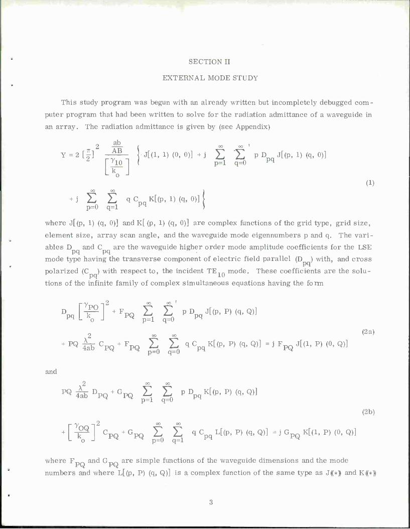
SECTION II
EXTERNAL MODE STUDY
This study program was begun with an already written but incompletely debugged com-
puter program that had been written to solve for the radiation admittance of a waveguide in
an array. The radiation admittance is given by (see Appendix)
2 — ( oo oo »
Y=2[|] -£^- [j[(l, 1) (0, 0)] +] £ *Z P D J[(p, 1) (q, 0)] r^lO] C P=l q=0 pq
L o J (1)
OO OO \
+ j L E qC K[(p, 1) (q, 0)] p=0 q=l Pq )
where j[(p, 1) (q, 0)] and K[ (p, 1) (q, 0)] are complex functions of the grid type, grid size,
element size, array scan angle, and the waveguide mode eigennumbers p and q. The vari-
ables D and C are the waveguide higher order mode amplitude coefficients for the LSE
mode type having the transverse component of electric field parallel (D ) with, and cross
polarized (C ) with respect to, the incident TE1Q mode. These coefficients are the solu-
tions of the infinite family of complex simultaneous equations having the form
•y -»2 oo oo Dpq[v] +FPQ £ 5 PDpqj[(P'P)(q'Q)]
+ ** 4aF CPQ + FPQ S £ q Cpq K[(P' P) <q> Q)] = j FPQ J[(1' P) <0' Q)] (2 a)
and
^^b^Q^PQ £> £ P Dpq K[(p, P) (q, Q)] ^ ^ p=l q=0 ^n
2
(2b)
[ Iff ] CPQ + GPQ ?0 S q Cpq L[(P> P) (q> Q)] = j GPQ K[(1> P) (0, Q)1
where Fpo and Gpo are simple functions of the waveguide dimensions and the mode
numbers and where L[(p, P) (q, Q)] is a complex function of the same type as J((*> and K((*))

above. The manner in which the waveguide modes have been defined allows us to designate
a mode as being of dominant polarization (MD) or of cross polarization (MC). In a waveguide
that is 0.6A. wide and 0.2667A. high, the modes are ordered by propagation constant as shown
in Table 1. It will turn out, however, that the final waveguide mode order will depend upon
the scan position in sine theta space rather than directly upon the waveguide propagation
constant.
The complex functions J((*)), K ((*)), and L((*)) have very similar forms, so that the
study of the convergence properties of any one of them is adequate for all three. The
simplest of the three was the one chosen for investigation. It is
OO 00-2 0
\—1 abk' o m=-°° n=-°°
(3)
• S (p) S (P) S (q) S (Q)
where
MW sin
S (p) = m^7 [¥-*]
m -w ß
m _ v L m\
ko B
ö - designate grid type mn r
X = sin 0cos <p
Y = sin 0 sin <f>

TABLE 1
ORDER OF THE WAVEGUIDE LSE MODES BY PROPAGATION CONSTANT
Dominant Cross Propagation Constant
p q MD. l
i =
MC. i
i =
v k
0
1 0 0 — jO.5527
2 0 1 — 1.3333
0 l — 1 1.5860
1 l 2 2 1.7916
3 0 3 — 2.2913
2 l 4 3 2.3007
3 l 5 4 2.9606
4 0 6 — 3.1797
0 2 — 5 3.6141
4 1 7 6 3.6914
1 2 8 7 3.7089
2 2 9 8 3.9799
5 0 10 — 4.0448
3 2 11 9 4.3945
5 1 12 10 4.4583
4 2 13 11 4.9166
5 2 14 12 5.5157
0 3 — 13 5.5353
1 3 15 14 5.5977
2 3 16 15 5.7807
3 3 17 16 6.0737
4 3 18 17 6.4614
0 4 — 18 7.4329
1 4 19 19 7.4795
2 4 20 20 7.6175

s -y
ZZI7 ^=7 a. Rectangular Grid
ZZ37
- / ^/yf /
-►X
^Z7
t Z
z^Z7
♦ ,' y y -7^ -►X
/ 7 / 7 b. Triangular Grid
ZZ37 / 7
Figure 1. Array Geometry
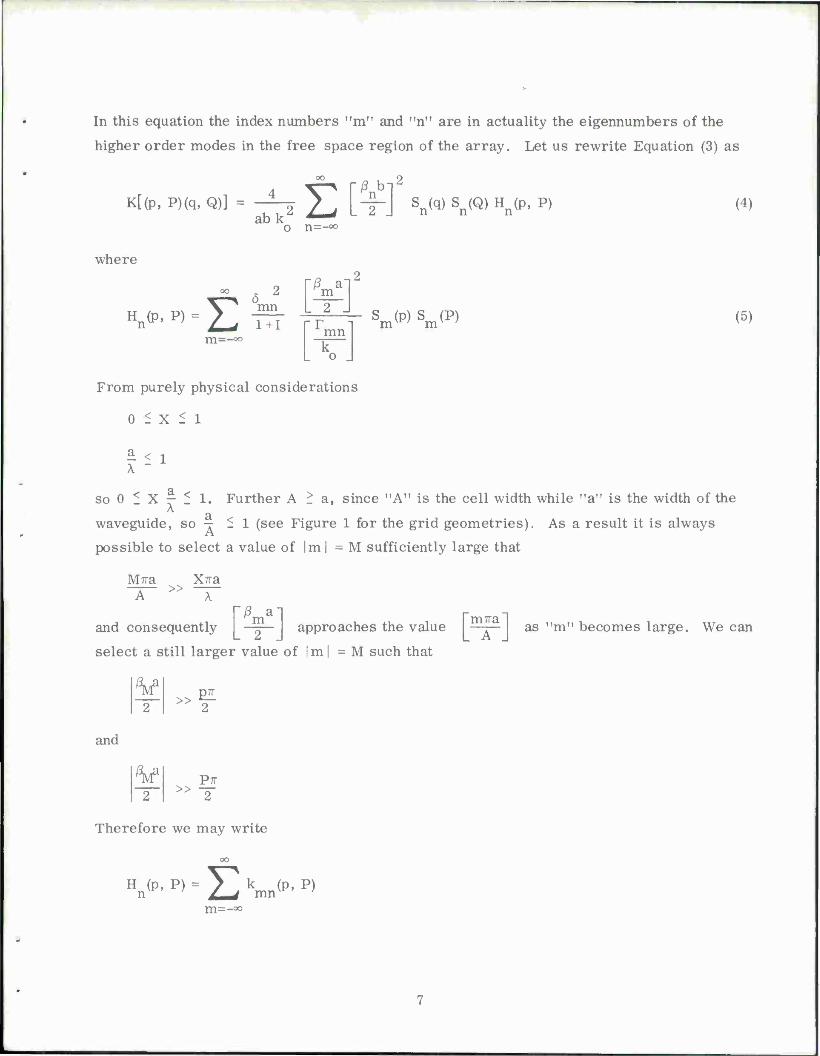
In this equation the index numbers "m" and "n" are in actuality the eigennumbers of the
higher order modes in the free space region of the array. Let us rewrite Equation (3) as
ß b^z
K[(p, P)(q, Q)] = ^2 J [-f-] Sn(q) Sn(Q) ^(p, P) (4)
o n=-°°
where
Hn(p, P) = ö 2
mn E m=-°°
m L 2 _
1+1 mn S (p) S (P) (5)
From purely physical considerations
0 < X < 1
Q
so 0 5 X — 5 1. Further A > a, since "An is the cell width while "a" is the width of the * a
waveguide, so 7 11 (see Figure 1 for the grid geometries). As a result it is always
possible to select a value of |m | = M sufficiently large that
M7ra X7ra
and consequently 'ß a ^m
L 2 . rm7ral approaches the value —r— as "m" becomes large. We can
select a still larger value of I m | = M such that
>> pjr
and
V >> P7T
Therefore we may write
Hn(p, P) = Ek (p, P) mnv '
m=-°o

-M M
X) kmn(P' P) + 2 kmn(P' P> + ]£ kmn^ P> m=-°o
AI
m=-M
m=-M m=M
k (p, P)
12 % > o cos
(6)
[jraj Z-^ 1 + 1
2m7ra 27rXa _ (p+P)7r COS I ——-
L A - COS (P-PK
m=M m :^
k _ o J
- 1
Consequently
Hn(P, P) Ä
M
m=-M
provided only that
Yu kmn(P> P)
M »
M »
pA 2a
PA 2a
since the sum on "m" from M to °° decreases at least as fast as l/M . For the summation
on MnM we have from pure physical considerations
0 < Y < 1
so 0 f Y — 5 1. Further B > b, since "B" is the height of the cell whereas "b" is the h
height of the encompassed waveguide, so ^ 5 1. As a result it is always possible to select
a value of In I = N sufficiently large that
NTrb Y?rb -BT^ —
and consequently I -y- approaches the value ^TD" as "n" becomes large. We can
select a still larger value of |n | = N such that

0Nb » SE
and
W » Q7T
Therefore we may write
K[(p, P)(q, Q)] =-f- S L^J k2ab
o n=-°o
ßj> Sn(q) Sn(Q) Hn(p, P)
k2ab o n=-°°
^ kn[(p, P)(q, Q)]
k2ab o
-N N
y^ kn[(p, P)(q, Q)] + ^2 kJ (P» p>ft' Q] n=-oo n=-N
^kn[(p, P)(q, Q)]
n=N
(7)
N
k ab . __ o * n=-N
J^ kn[(p, P)(q, Q)]
rBl2yHn^P)
L 7Tb J Z-/ 2
- COS
n=N
(q-Q)^
N
2n7rb cos cos 2?rYb (q+Q) !]
k ab o n=-N
2 kn[<P' P><q' Q>J

w.v.
0.018 42
-0.015 $ -0.006 SS: 0.001 x£x£ A0.004 ^vXy -0.000 xyvo.no |+ 57 S+ 38 = 63 S 63 /19
Figure 2. A Map of the Real Part of H (p, P) and the Number of Iterations (M)
Necessary for Convergence as a Function of p and P
10

provided only that
N »as. N »SS M » 2b , IN » 2b
q since the sum on "n" from N to °° decreases at least as fast as 1/N .
Equation (5) was programmed for computer solution and data was obtained for n = 0,
with a range for p and P from 0 to 7. The value of the sum was printed out for each value
of ± m to a maximum absolute value of M = 80, at each of 10 points in sine theta space.
For the purpose of evaluating the resulting mass of data, it was assumed that the accumu-
lated value of the sum at |m I =80 was the true value of the sum and that the sum had
converged at some smaller value of Im I if the attained value were within 0. 01 percent of
the final value. Figure 2 is a map of the final value of the sum of Equation (5) and the
value of "M" at which it was assumed to have converged. Figure 2 is for a representative A B point in sine theta space (X = 0.3 = Y) for a rectangular grid having — = 0.667, — = 0.3333,
ab A A and rectangular waveguides having - = 0. 6 and - = 0.2667. Table 2 is a sample case for
A A which p = 1, P = 3. The conclusion that was drawn from the mass of data in general and
which is borne out by Figure 2 is that the maximum values for H (p, P) occur when p = P,
and are attained with relatively few terms. Large values for H (p, P) are obtained with
only a few terms when both p and P are 2 or less and if p ^ P. Smaller values are obtained
within a reasonable number of terms if p (or P) is zero or unity, when P (or p) is 3 or
greater. Insignificant values for the sum H (p, P) occur everywhere else but each requires
a very large number of terms. In the unshaded region it is easily seen that M need not
exceed 32 for all values of P less than or equal to 5.
11
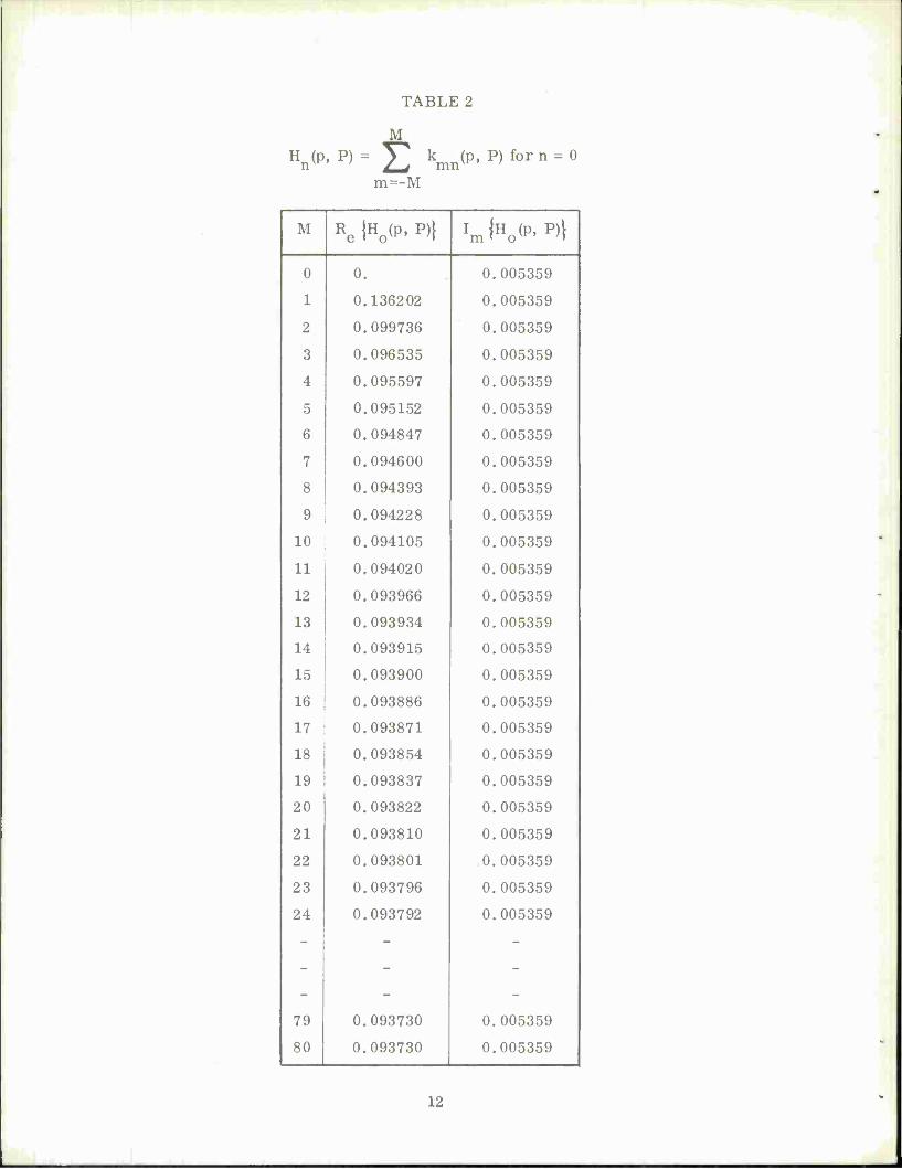
TABLE 2
M Hn(P' P) = 2 kmn(P' P) for n = °
m=-M
M Re lHo<P' P>1 ImlHo(P»P)l
0 0. 0.005359
1 0.136202 0.005359
2 0.099736 0.005359
3 0.096535 0.005359
4 0.095597 0.005359
5 0.095152 0.005359
6 0.094847 0.005359
7 0.094600 0.005359
8 0.094393 0.005359
9 0.094228 0.005359
10 0.094105 0.005359
11 0.094020 0.005359
12 0.093966 0.005359
13 0.093934 0.005359
14 0.093915 0.005359
15 0.093900 0.005359
16 0.093886 0.005359
17 0.093871 0.005359
18 0.093854 0.005359
19 0.093837 0.005359
20 0.093822 0.005359
21 0.093810 0.005359
22 0.093801 0.005359
23 0.093796 0.005359
24 0.093792 0.005359
79 0.093730 0.005359
80 0.093730 0.005359
12
-
SECTION III
STUDY OF THE MATRIX
Equation (3) exhibits a symmetry of form in m, p, P versus n, q, Q so that a function
H (q, Q) could have been considered instead of the H (p, P) given by Equation (5), and the
general results expressed above would have been essentially the same. Therefore, we may
expect the major values for K[(p, P)(q, Q)] of Equation (3) to occur when p = P and q = Q,
also when p, P, q, Q are all small (say ^ 2), and also when p (or P) and q (or Q) are either
zero or unity for larger values of P (or p) and Q (or q), say greater than 2. For all other
values of p, P, q, Q we may expect the value of K[(p, P)(q, Q)] to become almost vanishingly
small. If it is assumed that these other values of p, P, q, Q yield such small values that
they may justifiably be assumed to be identically zero, then the matrix for the left-hand side
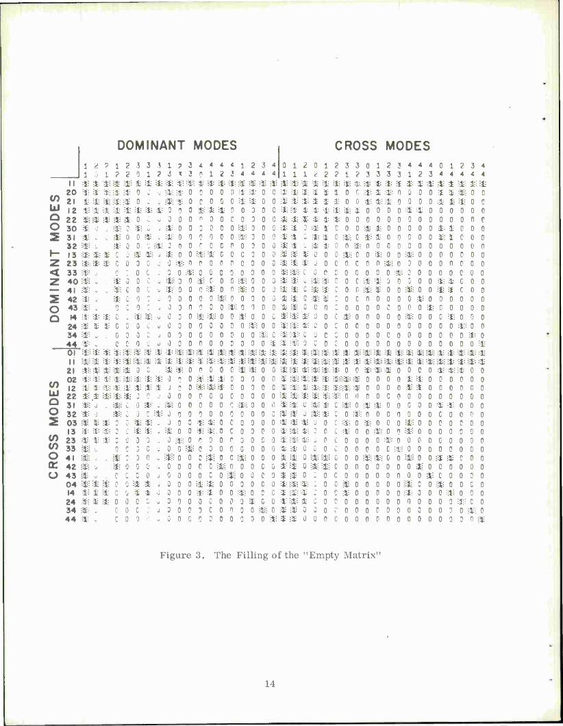
of Equations (2) will look like what is shown in Figure 3 where the O's and lfs denote "blank"
and "filled" matrix elements, respectively. Figure 3 was computed for 19 dominant (MD = 19)
and 20 cross (MC =20) modes inside the waveguide aperture. On this basis, of the 1521
possible elements only 533 need to be calculated. If it is assumed that all elements are
equally laborious to calculate, even if the value is vanishingly small, then there is a 65 per-
cent reduction in both time and labor in computing the matrix by retaining only the indicated
elements and by setting the other elements to zero.
Table 3 is a portion of the matrix for the left-hand side of Equations (2) where the upper
left quadrant is for the D^^ part of Equation (2a), the upper right is for the C^^. part of
Equation (2a), the lower left quadrant is for the D,,^ part of Equation (2b), and the lower
left is for the Cm part of Equation (2b). The portion of the matrix given was computed with
M equal to 30 for the same grid as is shown in Figure 2 and at the sine theta point X = 0.4 =Y.
The magnitude of the elements of the matrix bears out the expectation that the major values
should occur when p = P and q = Q. Most of the other values that are given are very small
except when p, P, q, Q are all small, for which case the elements are slightly larger, as is
also the case when p (or P) and q (or Q) are either zero or unity. This is also in keeping
with the expectation mentioned above.
There are some very interesting characteristics that show up in the matrix. Table 4 is
a list of the approximate absolute value of the elements along the main diagonal and along the
two subdiagonals of the matrix a part of which is shown in Table 3. Inspection of the table
will show that for the "dominant" modes there is a more or less constant value for the main
diagonal matrix element associated with a particular value of "p," regardless of the value
13
Id Q O
O Q
ÜJ Q O
C/) <n a <r o
DOMINANT MODES
ii 20 21 12 22 30 « 31 ft 32 «: 13 * 23 * 33 ft:
40 fti 41 BB 42 Üi 43 !$l 14 Ü
24 I« 34 $: 44 fti 01 II
21 02 12
&i fti; * :t
22 Ü 31 fti 32 m 03 ft 13 i 23 ft 33 a-j 41 fti 42 ft; 43 ft 04 fti 14 £ 24 & 34 & 44 *
i 7 1 0 1 2 * >$! Ü ii: £ ft ü; ü üi; & ü il ft ft *
; - fti w . ü
;* s c
i Hi v _ ft!
n
if: if; G Hi ü C - . 0
c if; üi *; ii ft * * Ü $ * ti 1 S; it; li i üi m u . ü; J fti Hi ft a 5:«; : * ft 3
0 - - ;*
g . C * * c £ ii c ii ft c
c c
2 3 2 0 Üi £ ft 0 ft o üi ü i 0 o si; 0 0 0 o J ft 0 3 : o 0 0 0 o 0 0 C 0 ; ii; 0 0 0 0 C 0
ft; ft m ft; ü o üi ü; ;li ft * J
0 0 C 0 o ü 0 ii 0 o 0 c 0 3
3 3 1 1 2 3 ü üi ü - . ft; : j ft;
* g; 0 : v o ü J i* ill J ü;
•j ft; 3 fti J Ü o j o C J 0 2 - m •J i ir : ü o : J o 3; u o C u 0 G J 0 G u 0
fti it ft ft ft ii
0 . Ü ü ü o Ü it J c - o ft . ft; : i# J
ii . J it; - ü 3 . 0 C « 0 o . m 0 v 0
? 3 * 3 *;ft; ft o Üi o
ft: 0 0 fti 3 0
m m ü m * o n 0 3 0 0 0 0 0 3 0 0 0 0 0 ft; o o ft; o o
J 0 i 0 0 3 ü 3 J 3
0 C
4 4 B 1 i ft 0 0 P 0 mm " 3 3 0 I? 0 c o ÜÜ
P 0 0 0 £ 0 0 1 0 0 0 3 ü ft;
G 0 C 0 P 0 ft ft S fti p o ill ft i*i Üi
P 0 0 0 0 0 Ü Si * ü: n 3 C 3 o m P 0 0 c ü ft Ü: Ü 3 c 3 C n 3
4 4 2 3 ü ü 0 0 0 0 ii o 0 P
C 0 0 0 0 0 üi o o ft o o 0 3 0 0 0 0 mm fti ft 0 c
o fti 0 c 0 0 P 0 0 n 0 0
1 2 3 4 4 4
ft ft ft ft ft 0 ü ü o 3 3 0 3 i 3 ft; 3 3 3 C 3 C 3 3 3 fti 3 3 .fti 3 C
0 3 3 3 0 0 Ü G 3 0 fti 3 o 3 ft; 3 3 B ü fti ft
ii ü G 3 3 0 3 3 3 m 3 3 3
3 3 0 3
m 3 3 0 3 C 3 0 C 3 3 C $; 3 3 3 Ü 3 3 0 ft: 3 3 3
CROSS MODES
ii ft 3 ft 3 ft c ü o ft 0 ii 0 ft o ü 3 ft 3 ü 3 S; 3 ft J ü i
1 2 3 in ü a 1 ü ü i ft ü i ft i ft Ü g $ Ü 3 :* i - ft * - ft ft li 3 ü ii: J
ft:: C ü m ^ ft: Ü C ii; ü 3 :*;
ft Ü 3 c Ü '■■i :i:
ü ft ft; ft
ö ü o J C 3i 3 ii il *
0 ft 3 ft 3 ü: 0 ü: o ft 3 a o i; 3 * 3 ü: C Ü G ft C ft Ü Ü
i-lii Ü Ü ft; ü e •{*;; C Ü fti 0 c ;ü; Ü: i3i; ü ü fti i3i 4i iii iiii ft: ft ill; ft ft; ü üi üi ft: ü fti ft J ft; ft ft: J fti (ti 3 ft; a; J ii 0 0 ft o ft; ;* o ;*: ft o ; ;ü; ft; : ft; ft : üi i ö iJ; 3 3 :Jt- 0 Ü
1 2 2 2 Ü Ü Ü 1 1 st
:i ;i; 1: ft i c Ü c
:i o 0 0 0 c P G ft D Ü C $ : o : 3 G 0 C c : o : ft ft ft; ft ü ii ii; m ii; m i; ft-; i c ii c 0 0 p 0
3 3 1 2 ii $: P G 0 0 ü; $ 0 3 0 0 ft: C P ii: fti c P c
Ü 3 0 P
t
c c
ü; G ii; C 3 C 0 G 0 C 0 G 3 C P C
0 G 0 0 ü ü ft ü o P
ft; ft ft; ft
p fi üi 3 o ft:
ft: 3 :ft P
P 0 P 0 D 3 ft ft
G C 0
0 3 ft Si i: o o it ti n o n o ft ft: n P n P P o
&; ii ii: c 0 P ft 0 $; o 0 p ft:
P 3 P 0 0 n p
3 4 3 1 ii & 0 0 9 3 3 ft 0 3 0 0 0 3 P 3 0 fti 0 3
£i 3 0 0 p ft; 0 3 0 P 0 fti 0 o 0 0 0 0 iii: Ü! ft; * 0 3
4 4 2 3 i ft 0 3
ü o 3 ii; 0 0 0 G 0 0 0 0 fti ft; SEI C 0
0 1 2 4 4 4
ft i üi it ü fti ü i ü 0 G 0 0 0 0 * li 0 li; I G 0 0 0 G 0 P o n p 0 0 G ü; g c Ü :f C 3 3 C 0
3 4 4 4 ÜÜ 0 0
p ii; P üi G 0 üi 0
G iü 0 0 0 o o;ft p üi; G G 0 0 0 0
i; o o ü C 0
c 0
c i|i: o 0 0 iii: o G o 0 0 0 ii ii m fti ft Ü: ii 1?i ii GOG
0 0 I 0 0 0 0 0
ü iü o C 0 0 C 0 0
Hi; o o o ;ü o o 3 ü; 0 3 0 0 0 3
0 0 0 0 0 0 D 0 0 0 ii: 0 o ü :i:ft ft: ft
0 0 G
p 0 p p p p 0 0 G 0
C 0 C 0 G 0 ft: o n g
Figure 3. The Filling of the "Empty Matrix"
14

TABLE 3
ABSOLUTE VALUES OF THE ELEMENTS IN PART OF THE MATRIX
en
[V pq PQV 11 20 21 12 22 01 11 21 02 12 22 10
11
20
21
12
22
0.51 0.1
2.89
0.02
0.06
2.78
0.02
0.004
0.006
0.65
0.023
0.005
0.059
0.031
0.022
3.16
0.06
0.11
0.29
0.025
0.047
2.41
0.15
0.12
0.08
0.01
0.047
0.15
5.06
0.005
0.12
0.023
0.06
0.05
0.06
0.56
0.078
0.036
0.011
5.72
0.10
0.005
0.24
0.14
0.05
11.4
0.29
0.26
0.12
0.12
0.02
0.246
0.372
0.252
0.079
0.839
0.107
0.04
0.027
0.04
0.01
0.02
0.02
0.35
0.011
0.054
01
11
21
02
12
22
0.025
2.41
0.06
0.024
0.16
0.013
0.11
0.39
0.53
0.17
0.20
1.45
0.11
0.1
5.06
0.043
0.019
0.24
0.005
0.039
0.003
0.027
5.72
0.048
0.01
0.004
0.07
0.25
0.09
11.43
3.75 0.43
3.07
0.38
0.13
0.57
0.16
0.06
0.29
3.42
0.09
0.15
0.40
0.23
0.13
0.11
24.3
0.057
0.28
0.12
0.13
23.7
0.038
0.07
0.23
0.50
0.16
23.7
0.95
0.19
0.51
0.29
0.19
0.26
1.11 0.17

TABLE 4
APPROXIMATE MAIN AND SUBDIAGONAL MATRIX ELEMENT VALUES
PQ Main Diagonal
Both Subdiagonals Dominant Cross
01 — 3.75 —
11 0.51 3.07 2.41
20 2.89 — —
21 2.78 3.42 5.06
02 — 24.26 —
12 0.65 23.66 5.72
22 3.16 23.66 11.43
30 9.39 — —
31 8.78 3.9 7.91
32 9.56 23.78 17.21
03 — 57.73 —
13 0.63 56.66 8.74
23 3.26 56.76 17.47
33 9.75 56.96 26.25
40 18.56 — —
41 17.55 4.14 10.90
42 18.54 23.89 23.02
43 18.86 57.13 35.07
04 — 106.5 —
14 0.63 105.2 11.93
24 3.35 105.2 23.84
34 9.97 105.2 35.75
44 19.23 105.2 47.66
16
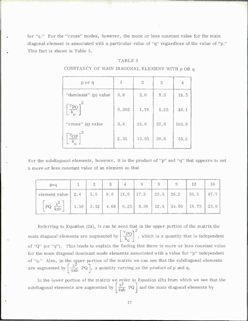
for "q." For the "cross" modes, however, the more or less constant value for the main
diagonal element is associated with a particular value of "q" regardless of the value of "p."
This fact is shown in Table 5.
TABLE 5
CONSTANCY OF MAIN DIAGONAL ELEMENT WITH p OR q
p or q 1 2 3 4
"dominant" (p) value 0.6 3.0 9.5 18.5
\[¥f 0.305 1.78 5.25 10.1 L o J
"cross" (q) value 3.8 24.0 57.0 105.0
"TOP" 2
2.51 13.05 30.6 55.2 L o J
For the subdiagonal elements, however, it is the product of "p" and "q" that appears to set
a more or less constant value of an element so that
p*q 1 2 3 4 6 8 9 12 16
eh 3ment val
x2 1 ^Äb.
ue 2.4
1.56
5.5
3.12
8.0
4.68
11.0
6.25
17.3
9.36
23.5
12.5
26.2
14.05
35.5
18.75
47.7
25.0
Referring to Equation (2a), it can be seen that in the upper portion of the matrix the i2
main diagonal elements are augmented by m- which is a quantity that is independent
of "Q" (or "q"). This tends to explain the finding that there is more or less constant value
for the main diagonal dominant mode elements associated with a value for "p" independent
of "q." Also, in the upper portion of the matrix we can see that the subdiagonal elements
are au gmented by -jV PQ , a quantity varying as the product of p and q.
In the lower portion of the matrix we refer to Equation (2b) from which we see that the r X2 1 subdiagonal elements are augmented by ^-r- PQ and the main diagonal elements by
17

TABLE 6
COMPARISON OF A FULL MATRIX WITH AN EMPTY MATRIX FOR A RECTANGULAR GRID ARRAY
4- = 0.6666, 5 = 0.3333, f = 0.6000, £ = 0.2666 A A A A
AT SINE THETA SPACE POINT
X = 0.500, Y = 0.750
p Q
Full Matrix Empty Matrix
G B G B
Dominant Mode Contribution
11 0 1.350472 0.012931 1.350472 0.012931
Principal Polarization Contribution
1 1 -0.398926 0.142121 -0.392068 0.132788
2 0 -0.021533 0.016890 -0.023566 0.016588
2 1 -0.588906 0.354161 -0.577752 0.344447
1 2 -0.039054 -0.013363 -0.036654 -0.011529
2 2 0.006181 -0.001933 0.003594 -0.001816
3 0 0.006367 0.003354 0.007999 -0.005562
3 1 0.007268 -0.001699 -0.004212 -0.008395
3 2 0.000152 0.000182 0.000187 -0.000224
1 3 -0.032859 0.005586 -0.031-12 0.005581
2 3 -0.076873 0.039342 -0.077453 0.038602
3 3 0.002627 0.000462 0.000232 -0.003091
Cross-Pol arization Contri buttons
0 1 -0.065360 0.090943 -0.068132 0.090361
1 1 0.035677 0.020559 0.035948 0.022415
2 1 -0.070353 0.266874 -0.069723 0.260815
0 2 0.000266 0.001105 -0.000260 0.000816
1 2 0.000852 0.004222 0.000353 0.004340
2 2 0. 000462 -0.002700 -0.000049 -0.001513
3 1 0.002122 -0.004717 -0.003549 -0.001461
3 2 0.000033 -0.000103 -0.000195 0.000073
0 3 -0.002189 0.002859 -0.000920 0.001242
1 3 0.003863 0.004180 0.003610 0.004183
2 3 -0.008335 0.038746 -0.008757 0.038766
3 3 0.000558 -0.001825 -0.002111 -0.000378
Total 0.112513 0.982060 0.105982 0.939979
18
m- 2
The augmentation of the subdiagonal elements is obviously again a product of p o
and q. The augmentation of the main diagonal elements in the lower portion of the matrix is
by a quantity which varies with Mq" and not with "p," and tends to explain the finding that
these elements appear to have a more or less constant value associated with a value of "q"
independent of the value of "p."
In both the upper and lower half of the matrix it can be seen that as "p" or "q" become
large, both the main diagonal as well as the subdiagonal elements tend to become quite large.
At the same time the element on the right-hand side of the equation tends to become small.
As a result, one can see that the amplitude coefficient for a mode having MpM or "q" large
can be expected to become relatively small. Therefore, it is reasonable to suppose that the
number of modes necessary to yield an adequately accurate answer should not be excessively
great.
The matrix emptying shown in Figure 3 was incorporated into the source program for
the main problem and tested. Then a sample case for a distant intercardinal point in sine
theta space was computed with both a filled matrix and an empty matrix for the simultaneous
equations of Equations (2). The result (by mode contribution) is shown in Table 6 for a rec- A B a
tangular grid having — = 0.6666, — = 0.3333, and waveguide dimensions - = 0.6000, i A A A
- = 0.2666, and assuming M = 25, at a sine theta position X = 0. 5, Y = 0. 75. Table 7 shows A
the overall result at four other points in sine theta space. It must be pointed out that the
values for mode contributions and the totals for the conductance and susceptance as given in
Tables 6 and 7 are incorrect because there was an error in the computer program by which
they were computed. That error, however, does not invalidate the comparison of the two
conditions of the same matrix since the error effects both conditions equally. It can be seen
from the two tables that (as expected) the empty matrix predicts an answer of very reason-
able accuracy as compared with the answer given by the full matrix. Comparison of the
modes used as shown in Table 6 with the form of the emptied matrix of Figure 3 shows that
the empty matrix solution is accomplished with about 57 percent of the time and labor that
was necessary for the full matrix solution. The emptied matrix method of solving the
simultaneous equations, however, is not without pitfalls because it is possible for it to pre-
dict a negative conductance in the near vicinity of an anomalous notch. This of course is
physically impossible, but it does indicate the very close proximity of a notch and one could
either accept it as being the notch, or rerun the region of the anomaly with a full matrix.
19
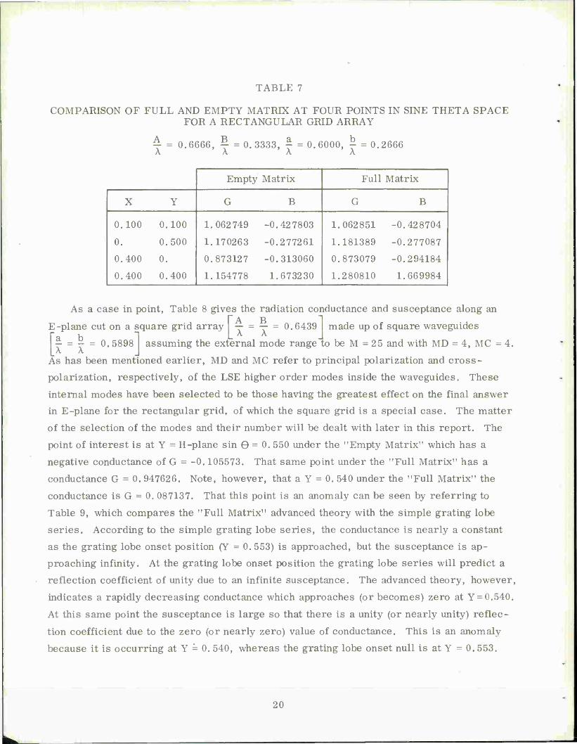
TABLE 7
COMPARISON OF FULL AND EMPTY MATRIX AT FOUR POINTS IN SINE THETA SPACE FOR A RECTANGULAR GRID ARRAY
4 = 0.6666, ^ = 0.3333, ^ = 0.6000, £ = 0.2666 A A A A
Empty Matrix Full Matrix
X Y G B G B
0.100 0.100 1.062749 -0.427803 1.062851 -0.428704
0. 0.500 1.170263 -0.277261 1.181389 -0.277087
0.400 0. 0.873127 -0.313060 0.873079 -0.294184
0.400 0.400 1.154778 1.673230 1.280810 1.669984
As a case in point, Table 8 gives the radiation conductance and susceptance along an [A B — = — = 0.6439 made up of square waveguides
A A = 0.5898 I assuming the external mode range to be M = 25 and with MD = 4, MC = 4.
As has been mentioned earlier, MD and MC refer to principal polarization and cross-
polarization, respectively, of the LSE higher order modes inside the waveguides. These
internal modes have been selected to be those having the greatest effect on the final answer
in E-plane for the rectangular grid, of which the square grid is a special case. The matter
of the selection of the modes and their number will be dealt with later in this report. The
point of interest is at Y = H-plane sin 0=0. 550 under the "Empty Matrix" which has a
negative conductance of G = -0.105573. That same point under the "Full Matrix" has a
conductance G = 0. 947626. Note, however, that a Y = 0. 540 under the "Full Matrix" the
conductance is G = 0. 087137. That this point is an anomaly can be seen by referring to
Table 9, which compares the "Full Matrix" advanced theory with the simple grating lobe
series. According to the simple grating lobe series, the conductance is nearly a constant
as the grating lobe onset position (Y = 0.553) is approached, but the susceptance is ap-
proaching infinity. At the grating lobe onset position the grating lobe series will predict a
reflection coefficient of unity due to an infinite susceptance. The advanced theory, however,
indicates a rapidly decreasing conductance which approaches (or becomes) zero at Y = 0.540.
At this same point the susceptance is large so that there is a unity (or nearly unity) reflec-
tion coefficient due to the zero (or nearly zero) value of conductance. This is an anomaly
because it is occurring at Y = 0. 540, whereas the grating lobe onset null is at Y =0.553.
20
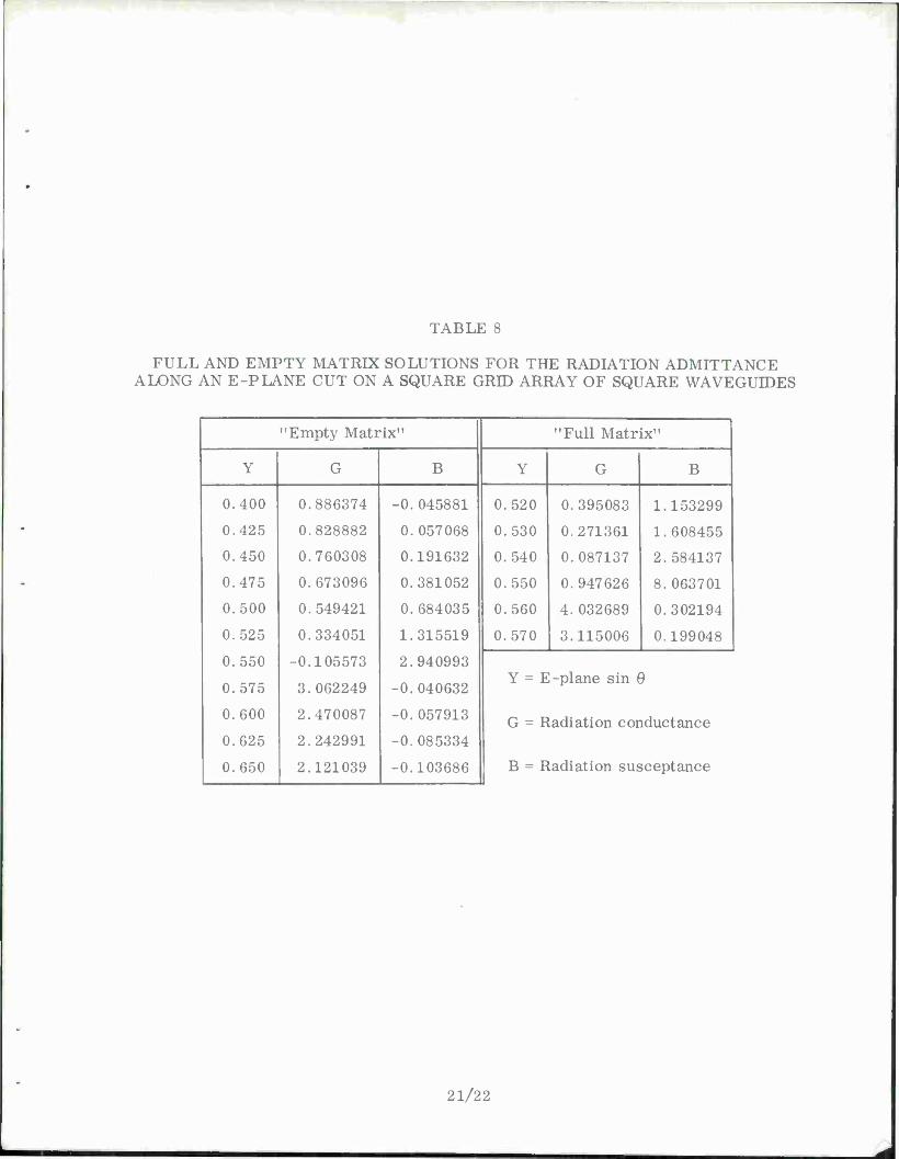
TABLE 8
FULL AND EMPTY MATRIX SOLUTIONS FOR THE RADIATION ADMITTANCE ALONG AN E-PLANE CUT ON A SQUARE GRID ARRAY OF SQUARE WAVEGUIDES
"Empty Matrix" "Full Matrix"
Y G B Y G B
0.400 0.886374 -0.045881 0.520 0.395083 1.153299
0.425 0.828882 0.057068 0.530 0.271361 1.608455
0.450 0.760308 0.191632 0.540 0.087137 2.584137
0.475 0.673096 0.381052 0.550 0.947626 8.063701
0.500 0.549421 0. 684035 0.560 4.032689 0.302194
0.525
0.550
0.334051
-0.105573
1.315519
2.940993
1 0.570 3.115006 0.199048
0.575 3.062249 -0.040632 Y = E-plane sin 9
0.600 2.470087 -0.057913 G = Radiation conductance 0.625 2.242991 -0.085334
0.650 2.121039 -0.103686 B = Radiation susceptance
21/22

SECTION IV
STUDY OF THE INTERNAL MODES
In all of the foregoing discussion no mention has been made concerning what waveguide
modes are necessary to adequately define the final admittance value. With an infinite num-
ber of simultaneous equations to select from for the solution for the mode amplitude coef-
ficients (D and C ) as expressed by Equations (2a) and (2b), the first problem is to include
enough of the higher order modes nearest cutoff in order that the solution of the truncated
set will give values that converge to very nearly the right answer. Prior knowledge of the
values for the coefficients or even their order of importance is completely unavailable.
Unfortunately, the form of the expressions encountered in Equations (2a) and (2b) does not
lend itself to analytically determining which modes are important or how many are needed
for an adequate answer.
At one point in the program it was decided to see if the equations — (2a) and (2b) —
should be reconstituted in terms of the TE and TM modes instead of the LSE modes. The
mode coefficients are related as follows.
D =KTE ^ + H ail pq L M
a pq b J
c =KTE ^-H K] pq L pq b PQ a J
(8)
where E and H are the mode amplitude coefficients for the pq TE and TM modes, pq pq F ^ respectively. The quantity K is one which could have been incorporated into E and H
The substitution of Equations (8) into (1), (2a), and (2b) is quite straightforward, but does
not lead to any simplification. On the contrary, the resulting equations are even more
unwieldy.
The next effort, directed toward finding an analytical convergence criterion for the
simultaneous equations, was an attempt to derive an expression that would relate the change
in the admittance to the change in the mode amplitude coefficients. If this is accomplished
by taking the derivative of Equations (1), (2a), and (2b) with respect to the coefficients,
considering the admittance to be a member of the group, the result is a matrix whose de-
terminant should approach a constant value as the number of modes is increased. This,
however, is almost identical to solving the matrix for Equations (2a) and (2b), substituting
the obtained values for the mode amplitude coefficients into Equation (1), and then insisting
that the admittance "Y" must approach a constant value. Consequently, this effort was also
abandoned.
23

TABLE 9
E-PLANE CUT ON A SQUARE GRID ARRAY OF SQUARE WAVEGUIDES; COMPARISON OF ADVANCED THEORY WITH THE SIMPLE GRATING LOBE SERIES
Simple Grating Lobe Series
Advanced Theory
Y G B G B
0.500 1.102326 0.0427453 - -
0.510 1.096260 0.563385 - -
0.520 1.090177 0.751856 0.395083 1.153299
0.530 1.084084 1.044166 0.271361 1.608455
0.540 1.077990 1.612427 0.087137 2.584137
0.550 1.071903 4.065890 0.947626 8.063701
0.560 4.017475 -0.439213 4.032689 0.302194
0.570 3.027679 -0.436978 3.115006 0.199048
0.580 2.668593 -0.434826 - -
0.590 2.472502 -0.432759 - -
0.600 2.346421 -0.430781 _ _
It was decided to attack the problem on a numerical basis. To do so, the defining
equations for the admittance and mode amplitude coefficients were programmed for computer
solution in such a way as to include the possibility of exciting all dominant polarization and
all cross-polarization higher order LSE waveguide modes which have either eigennumber of
the defining pair (p, q) equal to or less than 4 and including zero. As a consequence, there
are 19 "dominant" and 20 "cross" higher order modes to be considered inside the wave-
guides. In the array-space region is was decided, on the basis of the information presented
in the unshaded portion of Figure 2, that the range of the external eigennumbers should be
-30 < m < 30, -30 < n < 30 in order to adequately accommodate either internal eigennumber
(p or q) being equal to 4. This gives a total of 3721 external modes being taken into account.
24

The output data at each point in sine theta space consisted of the complex amplitude
coefficient for each mode and the associated contribution to the radiation admittance as well
as the absolute value of their product. Since the mode amplitude coefficient is essentially
equivalent to voltage, the product of mode amplitude coefficient and mode admittance con-
tribution has the units of current. This last was computed because it was felt that since the
mode contributions are essentially admittances in parallel, then those modes having the
greatest current would be the ones of greatest importance. That this concept is not valid
can be seen by considering the P, Q = 2, 4 mode which from Table 10 has an |AMP*Y I =
0.0637. Note that the mode P, Q = 1, 2 has an |AMP*Y| = 0.3632. If now the mode am-
plitude coefficients for these two modes are compared, we find that they are not too
different and, in fact, the former is the larger. Suppose a selection criterion were
assumed where only those modes having an | AMP*Y I greater than five percent of that of
the dominant mode (P, Q = 1, 0) were to be considered. Obviously the P, Q = 2, 4 mode
would be dropped from consideration. This, however, would be an error because Equations
(2) show that the amplitude of any one mode is a function of the values of all of the others.
Consequently, in any process of truncation of the infinite set of simultaneous equations, the
omission of any mode having a substantial amplitude coefficient will very adversely affect
the accuracy of all of the others, upon solution of the truncated set. The same argument
holds for rejecting the possible selection criterion based upon the amplitude of the mode
contribution to the radiation admittance.
The remaining quantity suitable for selection is the mode amplitude coefficient itself.
A few trial-and-error manipulations suggested that the best way to handle the selection was
to work with the square of the absolute value. That this is a pertinent choice may be recog-
nized by noting that the waveguide mode energy is equal to the square of the mode voltage
amplitude coefficient times the wave admittance, the latter of which is a quantity varying
approximately inversely as the propagation constant. Since, from Table 1, the propagation
constants for the modes of interest are all of roughly the same order, we can safely ignore
them for our purposes. Squaring the value automatically tends to enhance the larger ampli-
tude values and to very sharply suppress those that are small. It was decided to select on
the basis of the results obtained for the maximum number of modes that could be accommo-
dated by the available computer (IBM 7094). The computer runs were made at a single
point in each of H-plane, E-plane, and one intermediate plane for each of three grid sizes
25
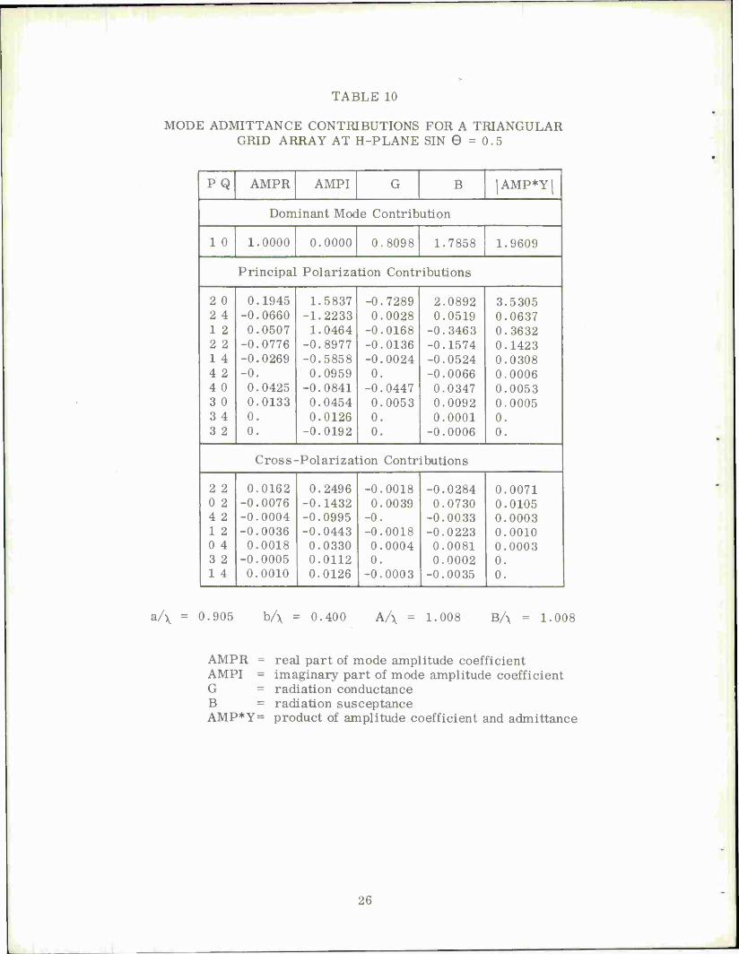
TABLE 10
MODE ADMITTANCE CONTRIBUTIONS FOR A TRIANGULAR GRID ARRAY AT H-PLANE SIN 0 = 0.5
PQ AMPR AMPI G B |AMP*Y|
Dominant Mode Contribution
1 0 1.0000 0.0000 0.8098 1.7858 1.9609
Principal Polarization Contributions
2 0 0.1945 1.5837 -0.7289 2.0892 3.5305 2 4 -0.0660 -1.2233 0.0028 0.0519 0.0637 1 2 0.0507 1.0464 -0.0168 -0.3463 0.3632 2 2 -0.0776 -0.8977 -0.0136 -0.1574 0.1423 1 4 -0.0269 -0.5858 -0.0024 -0.0524 0.0308 4 2 -0. 0.0959 0. -0.0066 0.0006 4 0 0.0425 -0.0841 -0.0447 0.0347 0.0053 3 0 0.0133 0.0454 0.0053 0.0092 0.0005 3 4 0. 0.0126 0. 0.0001 0. 3 2 0. -0.0192 0. -0.0006 0.
Cross-Polarization Contributions
2 2 0.0162 0.2496 -0.0018 -0.0284 0.0071 0 2 -0.0076 -0.1432 0.0039 0.0730 0.0105 4 2 -0.0004 -0.0995 -0. -0.0033 0.0003 1 2 -0.0036 -0.0443 -0.0018 -0.0223 0.0010 0 4 0.0018 0.0330 0.0004 0.0081 0.0003 3 2 -0.0005 0.0112 0. 0.0002 0. 1 4 0.0010 0.0126 -0.0003 -0.0035 0.
a/\ = 0.905 b/\ = 0.400 A/\ = 1.008 B/\ = 1.008
AMPR = real part of mode amplitude coefficient AMPI = imaginary part of mode amplitude coefficient G = radiation conductance B = radiation susceptance AMP*Y= product of amplitude coefficient and admittance
26

for both rectangular and triangular grid. For each plane, the values for each grid size
corresponding to a given mode were added, in order to obtain a composite value valid for
several grids and waveguide sizes. Doing this will also tend to average out small varia-
tions in the order for one grid size relative to another. The mode order for that scan plane
was determined by the value of that mode's sum in relation to the other mode sums. These
data are shown in Tables 11, 12, and 13 for the triangular grid and in Tables 15, 16, and 17
for the rectangular grid. Tables 14 and 18 are the final mode order for each of the three
scan planes for the triangular grid and the rectangular grid, respectively.
The problem at this point is to effectively use the data presented in Tables 14 and 18.
It was decided that if a value for a mode in the two tables above exceeded one percent of
the Dominant Mode (TE10) value of 3.0, then that mode should be included in the set for the
simultaneous solution of Equations (2) after truncation. This one percent level is indicated
by the short line in each column in both tables. The modes were accordingly incorporated
into the computer program. Table 10 is an excerpt from the 19 "dominant" and 20 "cross"
case for an H-plane point. Table 19 is a similar table for the same H-plane point except
that the modes are limited to those specified by Table 14 for the triangular grid. Table 10,
if it were all present, would give a total radiation admittance of Y = 0. 011997 + j 3. 429789.
Table 19 gives Y = 0. 030419 + j 3.238305. The difference between these amounts to an
error in the absolute value of less than six percent. For the same grid at an E-plane point
(x = o, y = 0.5), the 19 and 20 gives Y = 1.602131 + j 0.221731 and the modes of Table 14
give Y = 1. 594270 + j 0.219018. At an intercardinal point (x = 0.23, y = 0.23) not far from
the grating lobe circle, the results are, for the 19 and 20, Y = 0.283723 + j 1.826422 versus
Y = 0. 342088 + j 1. 329688 for the suggested number of modes. The error for the inter-
cardinal point is about 24.6 percent in the absolute value of the admittance. This could
easily be improved by including only a few more modes from the table for the mode order
(Table 14).
The suggested number of modes (Table 18) was tested by making an E-plane cut for a
rectangular grid as shown in Figure 4. This is the same array and the same cut that was
discussed in association with Tables 8 and 9 in the last paragraph of the previous section.
It was pointed out that the notch shown in Table 3 by the "Advanced Theory" is an anomalous
27

TABLE 11
TRIANGULAR GRID MODE COMPARISON BASED UPON MODE AMPLITUDE SQUARED FOR H-PLANE SCAN
X = H-plane sin 0
a/\=0.905,b/x=0.4 a/>=0.75,b/v=0.333 a/\=0.6364,b/\=0.2828 PQ A/\=1.008,B/\=1.008 A/\=0.8333, B/\=0.833 A/\=0.7071, B/>=0.7071 Sum*
X = 0.5, Y=0 X = 0.7, Y=0 X= 0.7, Y=0
Principal Polarization
1 1 0. 0. 0. 0. 2 0 2.5459 0.1258 0.0409 2.7126 1 2 1.0976 0.2608 0.1356 1.3993 3 0 0.0023 0.0029 0.0009 0.0061 1 3 0. 0. 0. 0. 1 4 0.3437 0.0912 0.0514 0.4863 3 1 0. 0. 0. 0. 2 2 0.8119 0.0605 0.0267 0.8991 2 1 0. 0. 0. 0. 4 0 0.0089 0.0020 0.0008 0.0117 2 4 1.5009 0.0063 0.0082 1.5154 3 2 0.0004 0. 0. 0. 4 1 0. 0. 0. 0. 3 3 0. 0. 0. 0. 2 3 0. 0. 0. 0. 4 2 0.0092 0.0035 0.0021 0.0148 3 4 0.0002 0.0004 0. 0.0006 4 3 0. 0. 0. 0.
Cross-Polarization
1 1 0. 0. 0. 0. 0 1 0. 0. 0. 0. 3 1 0. 0. 0. 0. 2 1 0. 0. 0. 0. 1 2 0.0020 0.0014 0.0001 0.0035 0 2 0.0205 0.0022 0.0009 0.0236 2 2 0.0626 0.0069 0.0029 0.0724 4 1 0. 0. 0. 0. 1 3 0. 0. 0. 0. 3 2 0.0001 0.0007 0. 0.0008 4 2 0.0099 0.0033 0.0016 9.0148 3 3 0. 0. 0. 0. 1 4 0.0002 0.0001 0. 0.0002 0 4 0.0011 0.0001 0. 0.0012 3 4 0. 0. 0. 0. 0 3 0. 0. 0. 0. 2 3 0. 0. 0.
0.
* Sum of the Three Grids PQ Mode Value
28
one because it is occurring inside of the grating lobe onset position and of the notch predicted
by the simple grating lobe series. Insofar as the experimental curve is concerned, all that
can be said is that the "Advanced Theory" agrees with the experiment better than does the
simple grating lobe series. This poor agreement may be due to the array being too small
even at 13 x 13.
The suggested number of modes (Table 14) was tested by making an H-plane cut for a
triangular grid, as shown in Figure 5. Here the anomalous notch is far enough inside the
H-plane onset position of the grating lobe that it is readily obvious. There are three
"Advanced Theory" predictions depicted on this figure, all of which predict a notch. The
curve for one dominant and no cross modes is with the TE~n mode only. The curve with
five dominant and one cross is the suggested list to the lines (Table 14), and the predicted
notch is somewhat farther out in sine theta space. The other curve is the first eight
dominant and the first seven cross from the suggested list and predicts a notch nearly like
that of the TE20 only. It is apparent from this result that selecting the modes only to the
one-percent level in Table 14 is inadequate to give a stationary prediction for the notch
even though the radiation admittance is relatively stationary.
29
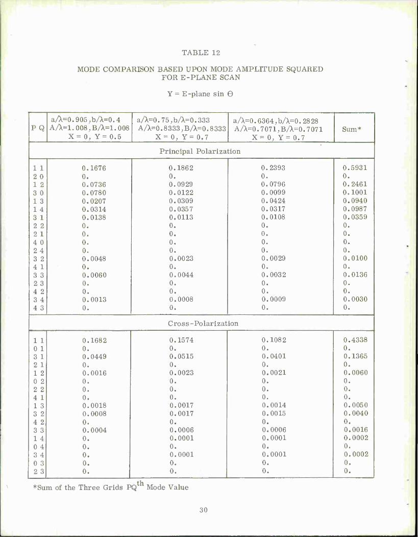
TABLE 12
MODE COMPARISON BASED UPON MODE AMPLITUDE SQUARED FOR E-PLANE SCAN
Y = E-plane sin 0
aA=0.905,b/X=0.4 a/X=0.75,b/X=0.333 a/X=0.6364,b/X=0.2828 PQ A/X=1.008,B/X=1.008 1 A/X=0.8333,B/X=0.8333 A/X=0.7071, B/X=0.7071 Sum*
X= 0, Y= 0.5 X= 0, Y= 0.7 X= 0, Y= 0.7
Principal Polarization
1 1 0.1676 0.1862 0.2393 0.5931 2 0 0. 0. 0. 0. 1 2 0.0736 0.0929 0.0796 0.2461 3 0 0.0780 0.0122 0.0099 0.1001
1 1 3 0.0207 0.0309 0.0424 0.0940 1 4 0.0314 0.0357 0.0317 0.0987 3 1 0.0138 0.0113 0.0108 0.0359 2 2 0. 0. 0. 0. 2 1 0. 0. 0. 0. 4 0 0. 0. 0. 0. 24 0. 0. 0. 0. 3 2 0.0048 0.0023 0.0029 0.0100 4 1 0. 0. 0. 0. 3 3 0.0060 0.0044 0.0032 0.0136 2 3 0. 0. 0. 0. 4 2 0. 0. 0. 0. 3 4 0.0013 0.0008 0.0009 0.0030 4 3 0. 0. 0. 0.
Cross -Polarization
1 1 0.1682 0.1574 0.1082 0.4338 0 1 0. 0. 0. 0. 3 1 0.0449 0.0515 0.0401 0.1365 2 1 0. 0. 0. 0. 1 2 0.0016 0.0023 0.0021 0.0060 0 2 0. 0. 0. 0. 2 2 0. 0. 0. 0. 4 1 0. 0. 0. 0. 1 3 0.0018 0.0017 0.0014 0.0050 3 2 0.0008 0.0017 0.0015 0.0040 4 2 0. 0. 0. 0. 3 3 0.0004 0.0006 0.0006 0.0016 14 0. 0.0001 0.0001 0.0002 04 0. 0. 0. 0. 3 4 0. 0.0001 0.0001 0.0002 0 3 0. 0. 0. 0. 2 3 0. 0. 0. 0.
*Sum of the Three Grids PQ Mode Value
30
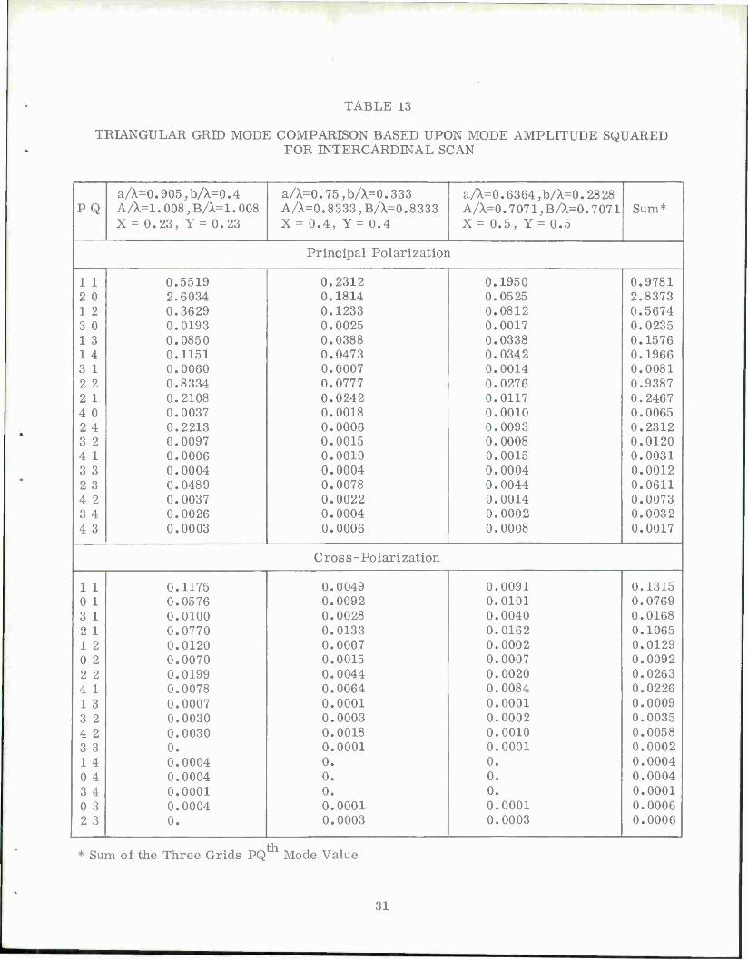
TABLE 13
TRIANGULAR GRID MODE COMPARISON BASED UPON MODE AMPLITUDE SQUARED FOR INTERCARDIN AL SCAN
a/X=0.905,b/X=0.4 1 a/X=0.75,b/X=0.333 a/X=0.6364,b/X=0.2828 PQ A/X=1.008,B/X=1.008 A/X=0.8333,B/X=0.8333 A/X=0.7071,B/X=0. 7071 Sum*
X = 0.23, Y= 0.23 X= 0.4, Y= 0.4 X = 0.5, Y= 0.5
Principal Polarization
1 1 0.5519 0.2312 0.1950 0.9781 2 0 2.6034 0.1814 0.0525 2.8373 1 2 0.3629 0.1233 0.0812 0.5674 3 0 0.0193 0.0025 0.0017 0.0235 1 3 0.0850 0.0388 0.0338 0.1576 14 0.1151 0.0473 0.0342 0.1966 3 1 0.0060 0.0007 0.0014 0.0081 2 2 0.8334 0.0777 0.0276 0.9387 2 1 0.2108 0.0242 0.0117 0.2467 4 0 0.0037 0.0018 0.0010 0.0065 24 0.2213 0.0006 0.0093 0.2312 3 2 0.0097 0.0015 0.0008 0.0120 4 1 0.0006 0.0010 0.0015 0.0031 3 3 0.0004 0.0004 0.0004 0.0012 23 0.0489 0.0078 0.0044 0.0611 4 2 0.0037 0.0022 0.0014 0.0073 3 4 0.0026 0.0004 0.0002 0.0032 4 3 0.0003 0.0006 0.0008 0.0017
Cross-Polarization
1 1 0.1175 0.0049 0.0091 0.1315 0 1 0.0576 0.0092 0.0101 0.0769 3 1 0.0100 0.0028 0.0040 0.0168 2 1 0.0770 0.0133 0.0162 0.1065 1 2 0.0120 0.0007 0.0002 0.0129 0 2 0.0070 0.0015 0.0007 0.0092 2 2 0.0199 0.0044 0.0020 0.0263 4 1 0.0078 0.0064 0.0084 0.0226 1 3 0.0007 0.0001 0.0001 0.0009 3 2 0.0030 0.0003 0.0002 0.0035 4 2 0.0030 0.0018 0.0010 0.0058 3 3 0. 0.0001 0.0001 0.0002 14 0.0004 0. 0. 0.0004 0 4 0.0004 0. 0. 0.0004 3 4 0.0001 0. 0. 0.0001 0 3 0.0004 0.0001 0.0001 0.0006 2 3 0. 0.0003 0.0003 0.0006
* Sum of the Three Grids PQth Mode Value
31
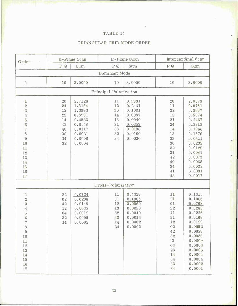
TABLE 14
TRIANGULAR GRID MODE ORDER
Order H-Plane Scan E-Plane Scan Intercardinal Scan
P Q Sum PQ Sum PQ Sum
Dominant Mode
0 10 3.0000 10 3.0000 10 3.0000
Principal Polarization
1 20 2.7126 11 0.5931 20 2.8373 2 24 1.5154 12 0.2461 11 0.9781 3 12 1.3993 30 0.1001 22 0.9387 4 22 0.8991 14 0.0987 12 0.5674 5 14 0.4863 13 0.0940 21 0.2467 6 42 0.0.48 31 0.0359 24 0.2312 7 40 0.0117 33 0.0136 14 0.1966 8 30 0.0061 32 0.0100 13 0.1576 9 34 0.0006 34 0.0030 23 0.0611
10 32 0.0004 30 0.0235 11 32 0.0120 12 31 0.0081 13 42 0.0073 14 40 0.0065 15 34 0.0032 16 41 0.0031 17 43 0.0017
Cross-Polarization
1 22 0.0724 11 0.4338 11 0.1315 2 3
02 42
0.0236 0.0148
31 12
0.1365 21 01
0.1065 0.0769 0.0060
4 12 0.0035 13 0.0050 22 0.0263 5 04 0.0012 32 0.0040 41 0.0226 6 32 0.0008 33 0.0016 31 0.0168 7 14 0.0002 14 0.0002 12 0.0129 8 34 0.0002 02 0.0092 9 42 0.0058
10 32 0.0035 11 13 0.0009 12 03 0.0006 13 23 0.0006 14 14 0.0004 15 04 0.0004 16 33 0.0002 17 34 0.0001
32

TABLE 15
RECTANGULAR GRID MODE COMPARISON BASED UPON MODE AMPLITUDE SQUARED FOR H-PLANE SCAN
X = H-plane sin 0
a/X=0.6,b/X=0.2667 a/X=0.5898,b/X=0.5898 a/X=0.6364,b/X=0.6364 PQ A/X=0.666,B/X=0.333 A/X=0.6439 ,B/X=0.6439 A/X=0.7071, B/X=0.7071 Sum*
X = 0.4, Y= 0 X= 0.5, Y= 0 X= 0.375, Y= 0
Principal Polarization
1 1 0. 0. 0. 0. 1 2 0.0155 0.0042 0.0058 0.0255 14 0.0083 0.0028 0.0037 0.0148 1 3 0. 0. 0. 0. 2 0 0.0069 0.0105 0.0412 0.0586 4 0 0.0002 0.0003 0.0003 0.0008 2 1 0. 0. 0. 0. 3 0 0.0014 0.0011 0.0017 0.0042 3 1 0. 0. 0. 0. 3 2 0. 0. 0. 0. 2 2 0.0001 0. 0. 0.0001 2 3 4 2 4 1 3 3 4 3 2 4 3 4
Cross -Polarization
1 1 0. 0. 0. 0. 3 1 0. 0. 0. 0. 1 2 0. 0. 0.0002 0.0002 0 1 2 1 3 2 4 1 1 4 2 2 0 2 1 3 3 3 3 4 2 3 4 2 0 3
1 4 3 |
♦Sum of the Three Grids PQ Mode Value
33
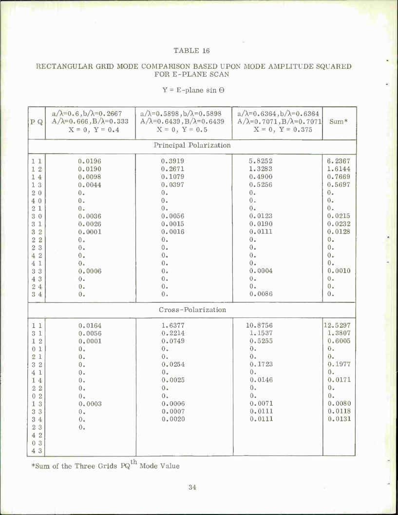
TABLE 16
RECTANGULAR GRID MODE COMPARISON BASED UPON MODE AMPLITUDE SQUARED FOR E-PLANE SCAN
Y = E-plane sin 9
a/X=0.6,b/X=0.2667 a/X=0.5898,b/X=0.5898 a/X=0.6364,b/X=0.6364 PQ A/X=0.666,B/X=0.333 A/X=0.6439, B/X=0.6439 A/X=0.7071,B/X=0.7071 Sum*
X= 0, Y= 0.4 X= 0, Y= 0.5 X= 0, Y= 0.375
Principal Polarization
1 1 0.0196 0.3919 5.8252 6.2367 1 2 0.0190 0.2671 1.3283 1.6144 14 0.0098 0.1079 0.4900 0.7669 1 3 0.0044 0.0397 0.5256 0.5697 2 0 0. 0. 0. 0. 4 0 0. 0. 0. 0. 2 1 0. 0. 0. 0. 3 0 0.0036 0.0056 0.0123 0.0215 3 1 0.0026 0.0015 0.0190 0.0232 3 2 0.0001 0.0016 0.0111 0.0128 2 2 0. 0. 0. 0. 2 3 0. 0. 0. 0. 4 2 0. 0. 0. 0. 4 1 0. 0. 0. 0. 3 3 0.0006 0. 0.0004 0.0010 4 3 0. 0. 0. 0. 24 0. 0. 0. 0. 3 4 0. 0. 0.0086 0.
Cross-Polarization
1 1 0.0164 1.6377 10.8756 12.5297 3 1 0.0056 0.2214 1.1537 1.3807 1 2 0.0001 0.0749 0.5255 0.6005 0 1 0. 0. 0. 0. 2 1 0. 0. 0. 0. 3 2 0. 0.0254 0.1723 0.1977 4 1 0. 0. 0. 0. 1 4 0. 0.0025 0.0146 0.0171 2 2 0. 0. 0. 0. 0 2 0. 0. 0. 0. 1 3 0.0003 0.0006 0.0071 0.0080 3 3 0. 0.0007 0.0111 0.0118 3 4 0. 0.0020 0.0111 0.0131 2 3 0. 4 2 0 3 4 3
*Sum of the Three Grids PQ Mode Value
34
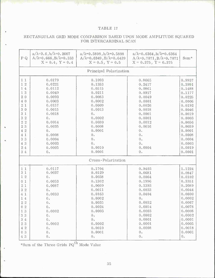
TABLE 17
RECTANGULAR GRID MODE COMPARISON BASED UPON MODE AMPLITUDE SQUARED
- FOR INTERCARDINAL SCAN
a/X=0.6,b/X=0.2667 a/X=0.5898,b/X=0.5898 a/X=0.6364,b/X=0.6364 PQ A/X=0.666,B/X=0.333
X = 0.4, Y= 0.4 A/X=0.6349, B/X=0.6439
X = 0.5, Y= 0.5 A/X=0.7071,B/X=0.7071 X= 0.375, Y= 0.375
Sum*
Principal Polarization
1 1 0.0179 0.1093 0.8665 0.9937 1 2 0.0221 0.1353 0.2417 0.3991 1 4 0.0112 0.0515 0.0861 0.1488 1 3 0.0049 0.0211 0.0917 0.1177 2 0 0.0093 0.0083 0.0049 0.0225 4 0 0.0003 0.0002 0.0001 0.0006 2 1 0.0157 0.0009 0.0026 0.0192 3 0 0.0015 0.0013 0.0018 0.0046 3 1 0.0018 0. 0.0001 0.0019 3 2 0. 0.0002 0.0001 0.0003 2 2 0.0014 0.0030 0.0012 0.0056
t. 2 3 0.0035 0.0008 0.0016 0.0059 4 2 0. 0.0001 0. 0.0001 4 1 0.0008 0. 0. 0.0008 3 3 0.0004 0. 0. 0.0004 4 3 0.0003 0. 0. 0.0003 24 0.0005 0.0010 0.0004 0.0019 3 4 0. 0.0001 0. 0.0001
Cross-Polarization
1 1 0.0117 0.1704 0.9403 1.1224 3 1 0.0037 0.0129 0.0681 0.0847 1 2 0. 0.0038 0.0064 0.0102 0 1 0.0053 0.1302 0.1996 0.3351 2 1 0.0087 0.0609 0.1393 0.2089 3 2 0. 0.0011 0.0033 0.0044 4 1 0.0033 0.0163 0.0404 0.0600 1 4 0. 0.0002 0. 0.0002 2 2 0. 0.0035 0.0032 0.0067 0 2 0. 0.0024 0.0054 0.0078 1 3 0.0002 0.0003 0.0003 0.0008 3 3 0. 0. 0.0002 0.0002 3 4 0. 0. 0.0001 0.0001 2 3 0.0002 0.0002 0.0001 0.0005 4 2 0. 0.0010 0.0008 0.0018 0 3 0. 0.0001 0. 0.0001 4 3 0. 0. 0. 0.
- *Sum of the Three Grids PQ1 Mode Value
35
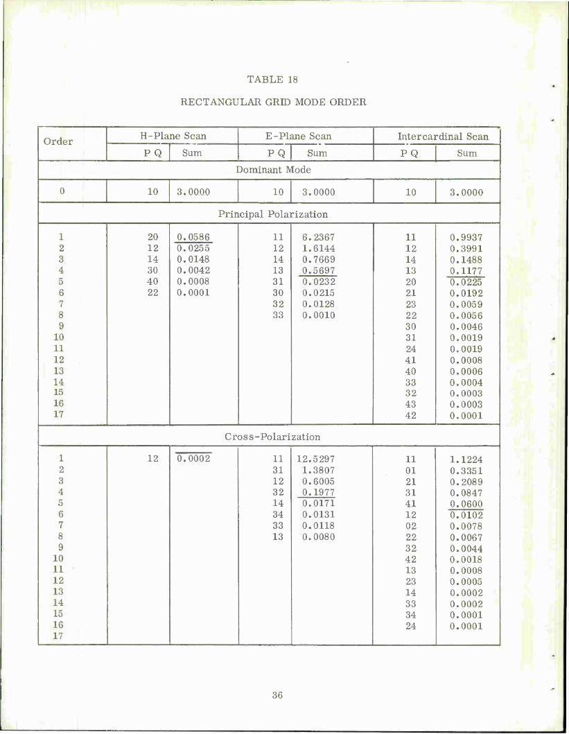
TABLE 18
RECTANGULAR GRID MODE ORDER
Order H-Plane Scan E-Plane Scan Inter cardinal Scan
PQ Sum PQ Sum PQ Sum
Dominant Mode
0 10 3.0000 10 3.0000 10 3.0000
Principal Polarization
1 2
20 12
0.0586 11 12
6.2367 1.6144
11 12
0.9937 0.3991 0.0255
3 14 0.0148 14 0.7669 14 0.1488 4 30 0.0042 13 0.5697 13 0.1177 5 40 0.0008 31 0.0232 20 0.0225 6 22 0.0001 30 0.0215 21 0.0192 7 32 0.0128 23 0.0059 8 33 0.0010 22 0.0056 9 30 0.0046
10 31 0.0019 11 24 0.0019 12 41 0.0008 13 40 0.0006 14 33 0.0004 15 32 0.0003 16 43 0.0003 17 42 0.0001
Cr oss-Polarization
1 12 11 12.5297 11 1.1224 0.0002 2 31 1.3807 01 0.3351 3 12 0.6005 21 0.2089 4 32 0.1977 31 0.0847 5 14 0.0171 41 0.0600 6 34 0.0131 12 0.0102 7 33 0.0118 02 0.0078 8 13 0.0080 22 0.0067 9 32 0.0044
10 42 0.0018 11 13 0.0008 12 23 0.0005 13 14 0.0002 14 33 0.0002 15 34 0.0001 16 24 0.0001 17
36
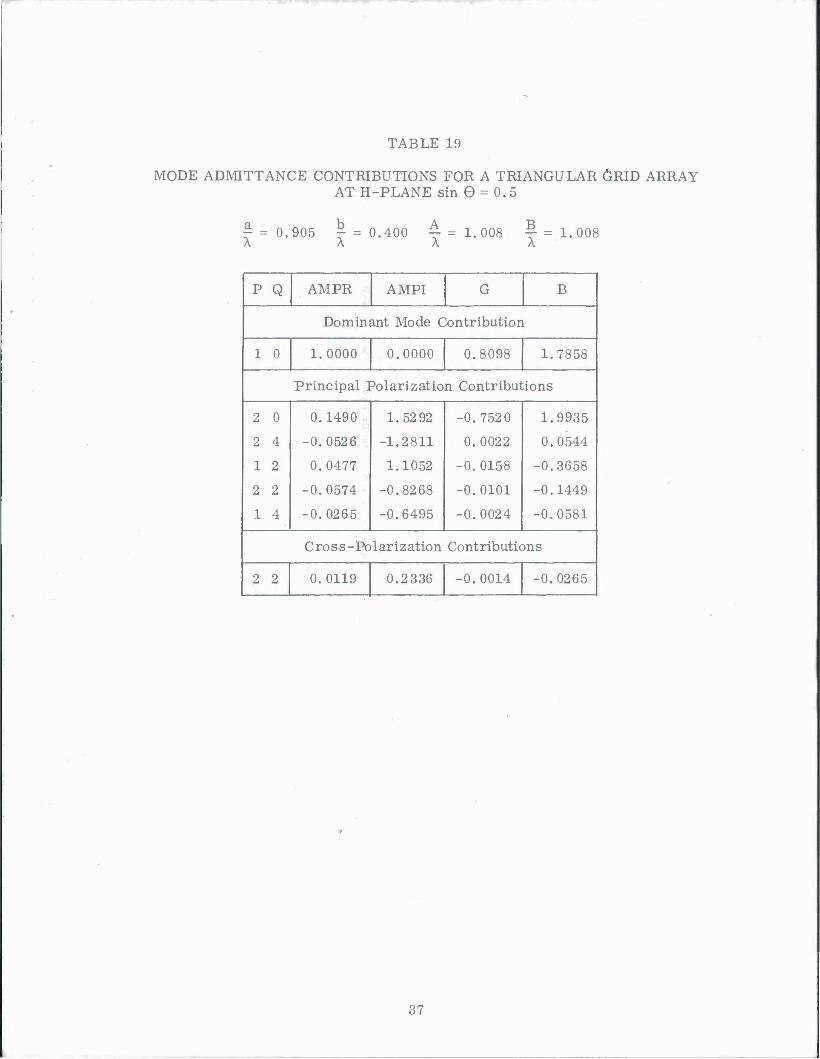
TABLE 19
MODE ADMITTANCE CONTRIBUTIONS FOR A TRIANGULAR ÖRID ARRAY AT H-PLANE sin 9 = 0.5
f = 0.905 ^=0.400 4=1.008 5. = 1.008 A A A A
P Q AMPR AMPI G B
Dominant Mode Contribution
1 0 1.0000 0.0000 0.8098 1.7858
Principal Polarization Contributions
2 0
2 4
1 2
2 2
1 4
0.1490
-0.0526
0.0477
-0.0574
-0.0265
1.5292
-1.2811
1.1052
-0.8268
-0.6495
-0.7520
0.0022
-0.0158
-0.0101
-0.0024
1.9935
0.0544
-0.3658
-0.1449
-0.0581
Cross-Polarization Contributions
2 2 0.0119 0.2336 -0.0014 -0.0265
37

0.4 0.5 E- PLANE SIN 6
Figure 4. Comparison of Theory and Experiment for an E-Plane Scan of an Array of Square Waveguides on a Square Grid
38

I.
00
or UJ H
<
< or
0.3 0.4 0.5 H-PLANE (SINE THETA)
Figure 5. Comparison of Theory and Experiment for an H-Plane Scan of an Array of Rectangular Waveguides on a Triangular Grid
39/40
SECTION V
CONCLUSIONS
The waveguide higher order modes in the order of decreasing importance are given in
Tables 14 and 18 for triangular grid and rectangular grid, respectively. These tables were
compiled on the basis of the square of the absolute value of the mode amplitude coefficients
obtained from solutions of simultaneous equations having 19 dominant polarization and 20
cross-polarization modes. The short lines in the columns represent the one-percent level
as compared with the incident mode amplitude.
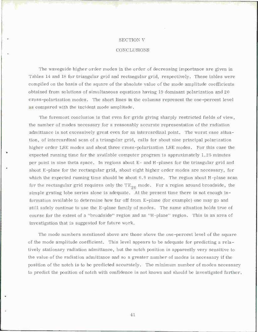
The foremost conclusion is that even for grids giving sharply restricted fields of view,
the number of modes necessary for a reasonably accurate representation of the radiation
admittance is not excessively great even for an intercardinal point. The worst case situa-
tion, of intercardinal scan of a triangular grid, calls for about nine principal polarization
higher order LSE modes and about three cross-polarization LSE modes. For this case the
expected running time for the available computer program is approximately 1.25 minutes
per point in sine theta space. In regions about E- and H-planes for the triangular grid and
about E-plane for the rectangular grid, about eight higher order modes are necessary, for
which the expected running time should be about 0.8 minute. The region about H-plane scan
for the rectangular grid requires only the TE 0 mode. For a region around broadside, the
simple grating lobe series alone is adequate. At the present time there is not enough in-
formation available to determine how far off from E-plane (for example) one may go and
still safely continue to use the E-plane family of modes. The same situation holds true of
course for the extent of a "broadside" region and an "H-plane" region. This is an area of
investigation that is suggested for future work.
The mode numbers mentioned above are those above the one-percent level of the square
of the mode amplitude coefficient. This level appears to be adequate for predicting a rela-
tively stationary radiation admittance, but the notch position is apparently very sensitive to
the value of the radiation admittance and so a greater number of modes is necessary if the
position of the notch is to be predicted accurately. The minimum number of modes necessary
to predict the position of notch with confidence is not known and should be investigated further.
41

The analytical and numerical work concerning the range over which the external eigen-
numbers should extend shows that if an eigennumber of the pair for the internal waveguide
modes is equal to 4 then the associated external eigennumber should have a range of ±30.
At the present time, the available computer program is written to take the most conserva-
tive view that if any internal mode has either eigennumber of the pair equal to 4, then both
external eigennumbers should have a range of ±30 for all members of the matrix for the
simultaneous equations. For example, the matrix element for which P, Q = 4, 2 and p, q =
1, 2 is currently computed with -30 < n - 30 and so has 3720 terms in the double sum for
the element. Reference to Figure 2 indicates that with P = 4 and p = 1, then M = 14, so
-14 S m ^ 14, and with Q = 2 and q = 2 then N = 10 so -10 < n 5 10. So doing would give
only 609 terms in the double sum for that same element. This possible reduction in labor
and computer running time should be investigated further.
42
SECTION VI
REFERENCES
1. Edelberg, S., and Oliner, A.A., "Mutual Coupling Effects in Large Antenna Arrays:
Part I - Slot Arrays," IRE Transactions on Antennas and Propagation, Vol. AP-8,
pp. 286-297, May 1960.
2. Farrell, G.F. Jr., and Kuhn, D.H., "Mutual Coupling Effects of Triangular-Arrays
by Modal Analysis," IEEE Transactions on Antennas and Propagation, Vol. AP-14,
pp. 652-654, September 1966.
3. This experimental curve was furnished by courtesy of Lincoln Laboratory, Lexington,
Massachusetts.
43/44
APPENDIX A
DERIVATION OF THE MUTUAL COUPLING IN AN INFINITE ARRAY OF RECTANGULAR WAVEGUIDE HORNS
The problem is solved by constructing Fourier Series expansions in terms of the normal
modes for the field components in both the free space region and in the element waveguide.
Both TE and TM modes are required in the free space region to account for the total far-
field distribution (Ref. 1), and are included in the free space Fourier representation. For
completeness, both TE and TM modes are also included in the waveguide series expansion.
Fourier methods are then employed to enforce the continuity of the total fields across the
boundary of the face of the array.
The radiation admittance equation as obtained by this method consists of the so-called
grating lobe series for the dominant mode of the waveguide, plus correction terms. Each
correction term is the product of a higher order waveguide mode amplitude coefficient and
a series having a form similar to the grating lobe series. The higher order waveguide
mode amplitude coefficients are obtained from the solution of a family of simultaneous
equations which are derived concurrently with the admittance equation. It is obvious, there-
fore, that the problem may not be solved exactly, because in practice one is forced to
truncate the grating lobe series, and there is also a practical limit to the number of wave-
guide modes that one would with to consider. Fortunately, the range of eigennumbers over
which the grating lobe series needs to be summed is not excessively large, and only a few
waveguide modes need to be considered in order to obtain reasonable accuracy.
Figures la and lb show the rectangular array and triangular array, respectively. In
both cases the unit cell is outlined by a rectangle, the dimensions of which are the units of
the lattice periodicity in the two directions. Since the lattice is periodic, each mode of the
field in the free space region of the array has a form governed by Floquet's theorem. A
suitable form is
2mjrl . [. . 2n7r"| ,-j |> * ¥] x -J k + -=- y TT Z , y B I J mn ,. .. e L _J e L ^ Je (A-l)
where
k = k sin 0cos ib X o
k = k sin 0sin ib y o ^
k = |s
45
and where k A and k B are the phase shifts between adjacent lattice units in the x and y
directions, respectively.
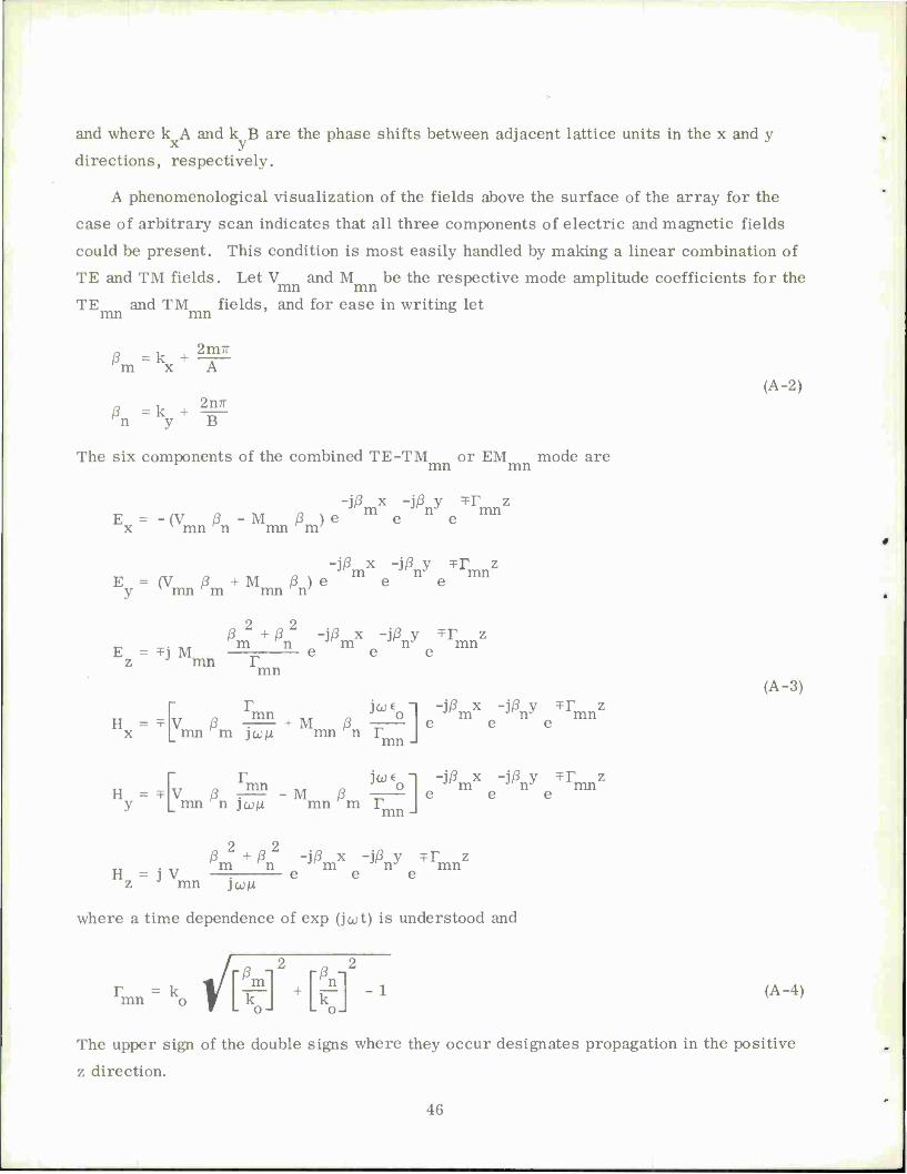
A phenomenological visualization of the fields above the surface of the array for the
case of arbitrary scan indicates that all three components of electric and magnetic fields
could be present. This condition is most easily handled by making a linear combination of
TE and TM fields. Let V and M be the respective mode amplitude coefficients for the mn mn ^ * TE and TM fields, and for ease in writing let mn mn ö
ß =k +^ m x A
ß -k + ^ n y B
The six components of the combined TE-TM or EM mode are ^ mn mn
-j/3 x -iß y TT z ^ /TT n Tv/r n v HI n mn E = - (V ß - M ß ) e e e x v mn Kn mn 'm'
-\ß x -iß y Tr z TI n a x m n mn
E=(V ß + M ß ) e e e y v mn m mn n7
ß 2 + ß2 -iß x -jß y *r z „ .. „ m Kn Ä
JMm JKnJ mn E = =FJ M —- e e e z J mn T mn
T jo;e 1 — i/3 x -j/3 y TT z ™M J ~ ' JKm JfnJ mn e e e j ß _*™ + M p _o mn'm JQ;M mn ^n Tmn J
H = =F V j3 ^ - M ß —-M y L1™1 n jw/x mn'm T J
r JOJ€ -i -j/3 x — jy3 y TT z e e e
mn
ß 2 + ß2 -iß x -iß y TT Z Mm Kn JAm *"nJ mn H = j V —: e e e
z J mn jcüM
where a time dependence of exp (jut) is understood and
*.-MW*Sf-'
(A-2)
(A-3)
(A-4)
The upper sign of the double signs where they occur designates propagation in the positive
z direction.
46

Six components of field can also be expected inside the aperture of the element wave-
guide, and will be treated as a linear combination of TE and TM modes with respective
mode amplitude coefficients E and H . The six field components have the form pq pq
E = -TE ^ - H H] COS ^ sin 9EL /W x _pqb pqa_ a b
E = [E EI + H f-~\ sin E* cos <&- e^ y |_ Pq a PQ b J a b
rELi2 + rai]2 Ty z
E =TH LsJ LbJ_staE«8togae M Z W ^pq a b
H = T X
y iw€ -l TV z n p7T 'pq __ q7r J r | . p7rx q7ry ^ rpq E ^- .-" + H %- sin ^— cos ^t~ e
pq a jcüM PQ b ypq J a b
[y - icü€ -i xy z _ q7r *pq __ p7r JW r I pro . q7iy + rpq E tr -r-" - H — cos ^— sin ~^- e HM
pq b jw/i Pq a y J a b
(A-5)
rEEi2 + rail2 Ty z H = -E i«4 ^ cos EH* cos SE e M
z pq jwjLt a b
relative to the lower left-hand corner of the element waveguide. A time dependence of
exp (jout) is understood, and
ypq = \ V[S]2 + ffi]a-r <A"6> where e is the relative dielectric constant in the waveguide.
It is assumed that energy is incident from inside the element waveguides with an ampli-
tude of unity and in the dominant TE mode having p = 1 and q = 0, and so the wave has its
"principal" polarization in the y-direction. It is further assumed that the wave is reflected
from the plane of the surface of the array with a voltage reflection coefficient R. The total
transverse field can now be written for the entire cross section represented by the array
space cell. It is assumed that the outline of the free space cell extends in both directions
from the face of the array.
47
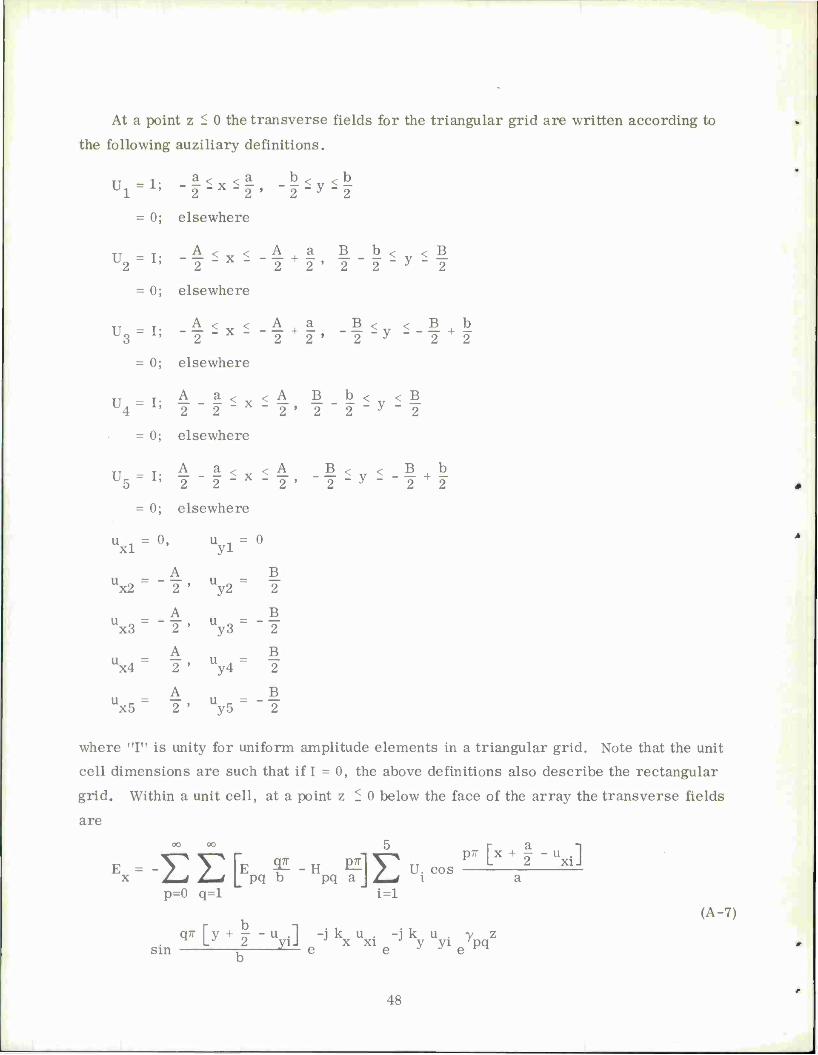
At a point z 5 0 the transverse fields for the triangular grid are written according to
the following auziliary definitions.
u1 = i
= 0
U2 = I
= 0
U3 = I
= 0
u4 = i
= 0
U5=I
_a<x <a _b<v <b 2~" "2 •
elsewhere
2 "y "2
_ £1 < B b < „ < B v x ^ - —- + — _ _ _ ^ v ^ —
elsewhere
B _A< < Aa B < < "2"X""2 2 ' ~ 2 ~y ~ 2 2
elsewhere
- - - < x < - 2 2
elsewhere
A 2
A i < < A 2 " 2 " X " 2
= 0; elsewhere
uxl = 0, uyl = 0
A B Ux2 2 ' Uy2 2
A B Ux3 ~ 2 ' Uy3 "2
A B Ux4 2 ' Uy4 2
A B Ux5 2 ■ Uy5 "2
B b < < B 2 " 2 " y " 2
_B< <_B+b 2 y 2 2
where "I" is unity for uniform amplitude elements in a triangular grid. Note that the unit
cell dimensions are such that if I = 0, the above definitions also describe the rectangular
grid. Within a unit cell, at a point z 5 0 below the face of the array the transverse fields
are
. cos x Z-rf L-J L pq b pq a J Z-rf i p=0 q=l i=l
q71" Ty + 77 - u .1 -j k u. -ik u. y z . n LJ 2 viJ x xi J v vi rPQ
p7r [x + f - uxi]
sin
(A-7)
48

[- 7. nz T- „z"l w-^ 7r | x + - - u . I -jku. -jku. e 10 + Re 10 J K-^2 u. sin -I ^—2ESi e X Xl e y yi
KX+f-Uxi]
E = e y L
i=l
oo oo t 5 r_ a
L~d L-J | pq a pq b J L-J I a p=l q=0 i=l
q71" I y + Ö - u .1 -iku. -iku. y z cos
Ly 2 Y±! e x X1 e y yl e pq
b
- 7- nz y.. nz~| y1 n —-^ 7T |~x + f- - u .1 -jku. -jku. H = - I e 10 - Re 10 J I 3 V U. sin -I ? Si e x xi e * * x L J a jojju Z—' i a
i=l
5
+ £-* Z—/ pq a JCJM pq b y Z—/ i a p=l q=0 pq i=l
q^Ty + ö - u -1 -j k u . -j k u . y z n LJ 2 viJ x xi J v vi 'PQ
(A-7)
cos . _Jiie X Xle y yiP
y Lf ZJ L pq b jwfi pq a y_ J Z-f i a p=0 q=l pq i=l
sin Q71" Ty + K ~ u -1 -jku. -jku. y z _. 1/ 2 viJ . x xi J v Vi PQ
where y y ^ signifies that the mode p=l, q=0 is to be excluded from the summation.
p=l q=0
The summations with "i" as the index accommodate the partial waveguide apertures at the
four corners of the unit cell in their proper phases relative to the waveguide at the center
of the cell by virtue of the definitions given above.
Within a unit cell, at a point z - 0 in the free space region above the face of the array,
the transverse fields are
JZ+ JZ- -j ß x -j ß y - r z E=TVrv ß -M ß le m e n e mn (A-8) x £ma ' * L mn ^n mn pmJ v '
—OO —OO
49
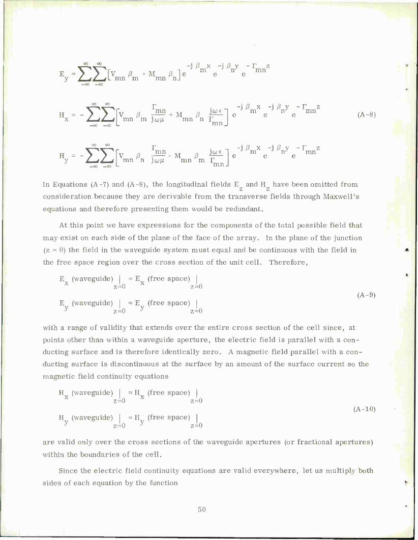
AA -jßx-jßy-r z T^ X^^Vir a , ix/r o 1 m n mn E = 7 7 V ß + M ß e e e y / JS J\ mn m mn nJ
H = - YT> /a ^ + M ^ ^1 e"3 ^ e"° ^ e" ^ (A-8) _oo -00 L mnj
H = -yy> ß J=5- y Z—/Z—rf mn ^n jcu/n mnrm T
—00 —00 •— n J
_ -3 /3 x -3 ß y - r z - M j3_ ^— I e e e
mn.
In Equations (A-7) and (A-8), the longitudinal fields E and H have been omitted from z z
consideration because they are derivable from the transverse fields through Maxwell's
equations and therefore presenting them would be redundant.
At this point we have expressions for the components of the total possible field that
may exist on each side of the plane of the face of the array. In the plane of the junction
(z = 0) the field in the waveguide system must equal and be continuous with the field in
the free space region over the cross section of the unit cell. Therefore,
E (waveguide) I = E (free space) x z=0 x z=0
(A-9) E (waveguide) = E (free space) I
y z=0 y z=0
with a range of validity that extends over the entire cross section of the cell since, at
points other than within a waveguide aperture, the electric field is parallel with a con-
ducting surface and is therefore identically zero. A magnetic field parallel with a con-
ducting surface is discontinuous at the surface by an amount of the surface current so the
magnetic field continuity equations
H (waveguide) = H (free space) x z=0 x z=0
(A-10) H (waveguide) = H (free space)
y z=0 y z=0
are valid only over the cross sections of the waveguide apertures (or fractional apertures)
within the boundaries of the cell.
Since the electric field continuity equations are valid everywhere, let us multiply both
sides of each equation by the function
50

j£rx )ßsy e e
orthogonal to the free space set, and integrate over the cell cross section. The result
of the integration on the free space side of the equations is zero except when r = m and
s = n, from which we obtain expressions for
V ß - M ß mn n mn m
and
V ß + M ß mn m mn n
from the E and E continuity equations, respectively. These are readily solved for
V and M , but first let us define the following functions, mn mn
Sm»>"
S„M ■
M-lfY
m2 - kf
(A-ll)
ö =1+1 cos mir cos n7r mn
where as before "I" is unity for a triangular grid and zero for a rectangular grid. As a
result
v - ' -^- ft mn " AB mn
. 7T 2 , ß ß -1 7T
<1 + R)[ä] ä 2 2 Sm'1'g.',"e
m n (A-12)
a ' m 2.2
~ oo oo
^y^y" TE 32L . H fill SE . s <p) S (q) e"J
- L-jL-J L pq b pq aj 2 m^' nVM/ 2 J 2
e
^m n p=0 q=l
^ OO OO j
u ß ß V"^X~^ + T-
m ^0 T^y TE ^ + H 9ll EL • s (p) S (q) e"3 g2 / J f J |_ pq a pq b J 2 mVF/ nVM/
'm+'n
_iE2L _iSE 2 J 2
e ] 51
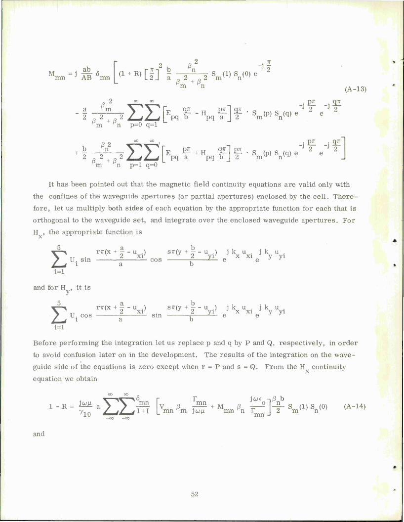
M = J TIT Ö mn J AB mn
2 ß2 -jS
<1+R>[f] I p7^ V1) Sn<°> e 2
m n (A-13)
a m X \ TT. Q71" TT P71" I q^ . o , v o , v 2 J 2 2 ^2 2
Mm pn p=0 q=l [E
Mf-«pq?]¥'=n,<P>V'>
pm n p=l q=0
It has been pointed out that the magnetic field continuity equations are valid only with
the confines of the waveguide apertures (or partial apertures) enclosed by the cell. There-
fore, let us multiply both sides of each equation by the appropriate function for each that is
orthogonal to the waveguide set, and integrate over the enclosed waveguide apertures. For
H , the appropriate function is x
5 a b X~^ r7T(x + - - u .) S7T(y + - - u .) jk u . jk u . V TT «<« 2 xi' _o u 2 yv J x xi J y yi / U. sin cos r *— e e J J
/ * i a b i=l
and for H , it is y
5 a b > . , . , Er7T(x + — - u .) S7T(y + — - u .) lk u. ik u. v 2 xr VJ 2 yr J x xi J y yi U. cos sin r J— e e J J
l a b i=l
Before performing the integration let us replace p and q by P and Q, respectively, in order
to avoid confusion later on in the development. The results of the integration on the wave-
guide side of the equations is zero except when r = P and s = Q. From the H continuity x equation we obtain
oo oo v "W ^ r r icü€ -iß b
1_R= mL&Y?jmL [v ß nm+M ß p>l-L s (1) S (0) (A-14) y10 / >/ -.l+T I mn pm )uß mnpn r J 2 mv ' nv
and
mn —oo —oo
52

^PQ a jo)M PQ b TpQ
<5 r r jw«-,0b P7T \~^ X ^ mn r,r o mn = j2tOQ 1~ . / * * ' i +T mn ^m JCJJU mn Kn r 2 v
P7T Q7T Jo J p
• S (P) S (Q) e * e mv ' nv '
where
£OQ = 1 ifQ = °
= 2 otherwise
From the H continuity equation we get
Qi !PQ H P* 3ctf<r ^PQ b jwM " PQ a ypQ
oo oo
-oo -oo
ö r- r iü;€ -> j3 a o r mn
a» » « > u,_ i cut -i p a. 7T X^ X mn |TT O mn ., 0
J o 1 m .. ifl,
-^ *-^ ^- 11111 "J
. P7T . Q7T J 2 J 2 S (P) S (Q) e e
mv ' nv '
where
,op = i ItP-O
= 2 otherwise
Let us now consider the substitution of V and M from Equations (A-12) and (A-13) mn mn into Equations (A-14), (A-15), and (A-16). After having done so, we can define anew pair
of amplitude coefficients.
_. p_7T . q7T
C =ä-J— rE 3ZL-H Ei-ie"] 2 e'J 2
pq 7T 1 + R L pq b pq a J v '
-i £ -j as. D = ä l rE EE + H SET e
2 e 2 (A-18) pq IT 1 + R L pq a pq b J
53

UNCLASSIFIED
Security Classification
DOCUMENT CONTROL DATA - R&D (Security classification of title, body of abstract and indexing annotation must be entered when the overall report is classified)
I. ORIGINATING ACTIVITY (Corporate author)
General Electric Company under P.O. No. C-487
2a. REPORT SECURITY CLASSIFICATION
I fnclassificd 2b. GROUP
None 3. REPORT TITLE
Mutual Coupling Study
4. DESCRIPTIVE NOTES (Type of report and Inclusive dates)
Technical Report
5. AUTHOR(S) (Last name, first name, initial)
Farrell, George F., Jr.
6. REPORT DATE
31 March 1967
7«. TOTAL NO. OF PAGES
64
7b. NO. OF REFS
3
8a. CONTRACT OR GRANT NO.
AF 19(628)-5167 b. PROJECT NO.
ARPA Order 498
9a. ORIGINATOR'S REPORT NUMBER(S)
GE Purchase Order No. EH-40039
9b. OTHER REPORT NO(S) (Any other numbers that may be assigned this report)
ESD-TR-67-279
10. AVAILABILITY/LIMITATION NOTICES
Distribution of this document is unlimited.
11. SUPPLEMENTARY NOTES
None
12. SPONSORING MILITARY ACTIVITY
Advanced Research Projects Agency, Department of Defense
13. ABSTRACT
This report gives the complete derivation (in an appendix) of the radiation admittance of a rectangular waveguide acting as an element in an infinite phased array. The derived equations are capable of predicting the experimentally observed anomalous notch that has been found to exist in arrays composed of large waveguides. The defining equations demonstrate that it is the existence of nonpropagating higher order modes inside the element waveguides that deter- mine the behavior of an infinite array.
It was the purpose of this study to determine what waveguide modes were important for a reasonably confident prediction of the radiation admittance of a rectangular waveguide in an array. It is shown that the number of modes needed for this is not excessively great, but that more are needed if it is desired to predict the position of an anomalous notch with any great degree of confidence.
14. KEY WORDS
phased arrays waveguide couplers rectangular waveguide
UNCLASSIFIED
Security Classification


GENERAL ELECTRIC