anomalous rainfall over southwest western australia …web.maths.unsw.edu.au/~alexg/pubs/anomalous...

Anomalous Rainfall over Southwest Western Australia Forced by Indian Ocean SeaSurface Temperatures

CAROLINE C. UMMENHOFER AND ALEXANDER SEN GUPTA

Climate Change Research Centre, University of New South Wales, Sydney, New South Wales, Australia

MICHAEL J. POOK

Centre for Australian Weather and Climate Research, CSIRO, Hobart, Tasmania, Australia

MATTHEW H. ENGLAND

Climate Change Research Centre, University of New South Wales, Sydney, New South Wales, Australia

(Manuscript received 11 September 2007, in final form 19 December 2007)

ABSTRACT

The potential impact of Indian Ocean sea surface temperature (SST) anomalies in modulating midlati-tude precipitation across southern and western regions of Australia is assessed in a series of atmosphericgeneral circulation model (AGCM) simulations. Two sets of AGCM integrations forced with a seasonallyevolving characteristic dipole pattern in Indian Ocean SST consistent with observed “dry year” (PDRY) and“wet year” (PWET) signatures are shown to induce precipitation changes across western regions of Australia.Over Western Australia, a significant shift occurs in the winter and annual rainfall frequency with thedistribution becoming skewed toward less (more) rainfall for the PDRY (PWET) SST pattern. For southwestWestern Australia (SWWA), this shift primarily is due to the large-scale stable precipitation. Convectiveprecipitation actually increases in the PDRY case over SWWA forced by local positive SST anomalies. Amechanism for the large-scale rainfall shifts is proposed, by which the SST anomalies induce a reorgani-zation of the large-scale atmospheric circulation across the Indian Ocean basin. Thickness (1000–500 hPa)anomalies develop in the atmosphere mirroring the sign and position of the underlying SST anomalies. Thisleads to a weakening (strengthening) of the meridional thickness gradient and the subtropical jet during theaustral winter in PDRY (PWET). The subsequent easterly offshore (westerly onshore) anomaly in the thermalwind over southern regions of Australia, along with a decrease (increase) in baroclinicity, results in thelower (higher) levels of large-scale stable precipitation. Variations in the vertical thermal structure of theatmosphere overlying the SST anomalies favor localized increased convective activity in PDRY because ofdifferential temperature lapse rates. In contrast, enhanced widespread ascent of moist air masses associatedwith frontal movement in PWET accounts for a significant increase in rainfall in that ensemble set.

1. Introduction

The seasonal to interannual variability in precipita-tion in the midlatitudes is generally assumed to be pre-dominantly driven by internal atmospheric dynamics.In contrast to the strong air–sea coupling in the tropics,the ocean’s role in forcing extratropical atmosphericvariability is often regarded to be of minor importance.

Kushnir et al. (2002) review the present understandingof the extratropical ocean’s role in modulating atmo-spheric circulation. They find that in addition to a directthermal response in the atmospheric boundary layer tosea surface temperature (SST) anomalies, there is alsoevidence for a significant modulation of the large-scaleatmospheric circulation. However, relative to the atmo-sphere’s internal variability the ocean-induced changesare small. Nevertheless, a wealth of studies have beeninspired by the possibility of utilizing the longer persis-tence of anomalies in the ocean, which in turn mightmodulate extratropical atmospheric variability, for im-proving seasonal to interannual climate forecasts

Corresponding author address: Caroline Ummenhofer, ClimateChange Research Centre, School of Mathematics and Statistics,University of New South Wales, Sydney, NSW 2052, Australia.E-mail: [email protected]

1 OCTOBER 2008 U M M E N H O F E R E T A L . 5113

DOI: 10.1175/2008JCLI2227.1

© 2008 American Meteorological Society

JCLI2227

(Kushnir et al. 2002, and references therein). A few ofthese studies show clear evidence that the extratropicalocean has a major effect on the large-scale atmosphericcirculation (e.g., Czaja and Frankignoul 1999; Rodwellet al. 1999; Sterl and Hazeleger 2005). Many more stud-ies demonstrate the overriding importance of the atmo-sphere’s internal variability, particularly in controllingprecipitation on interannual to seasonal time scales(e.g., Harzallah and Sadourny 1995; Rowell 1998;Watterson 2001). There is general agreement that amarked contrast exists between the tropics, where60%–80% of climate variability is SST forced, and themidlatitudes, where only about 20% can be attributedto SST forcing (Kushnir et al. 2002). In this study, wepresent evidence for regional midlatitude precipitationbeing significantly affected by extratropical SST on sea-sonal to interannual time scales in an atmospheric gen-eral circulation model (AGCM). This study is moti-vated by previous observational and modeling work byEngland et al. (2006), who find that precipitation oversouthwest Western Australia (SWWA) can be linked toa recurring SST dipole pattern in the Indian Ocean.

The first proposed link between Australian rainfallvariability and SST was made by Priestley and Troup(1966) and further explored by Streten (1981, 1983).Nicholls (1989) describes a gradient in SST between theIndonesian region and the central Indian Ocean that ishighly correlated with winter rainfall, extending fromthe northwest to the southeast of Australia. However,he cautioned against assuming causality, that is, that theSST pattern was forcing the rainfall changes. To deter-mine whether SST anomalies could be regarded as thecause of rainfall variations, Voice and Hunt (1984) car-ried out AGCM experiments where the atmospherewas forced by SST anomalies similar to those found byStreten (1981, 1983). However, they find conflicting re-sults, especially in the southern regions of Australia.Frederiksen et al. (1999) use multidecadal AGCMsimulations forced with observed global SST to split therainfall variance over Australia into components result-ing from SST forcing and internal variability. In theirexperiments, the SST forcing seems to be most influen-tial over the tropical northern part of the country.Ansell et al. (2000) find that observed rainfall in south-ern regions of Australia has a stronger link with varia-tions in mean sea level pressure (MSLP) than with In-dian Ocean SST. However, Frederiksen and Balgovind(1994) use an enhanced SST gradient reminiscent of theone described by Nicholls (1989) in AGCM simulationsand record an increased frequency of northwest cloudbands and associated winter rainfall over an area ex-tending from the northwest to the southeast of thecountry. For similar regions over Australia, Ashok et

al. (2003) link positive Indian Ocean dipole (IOD)events with a reduction in winter rainfall leading to abaroclinic response in the atmosphere resulting inanomalous subsidence. Applying an enhanced meridi-onal SST gradient in the eastern Indian Ocean, Fred-eriksen and Frederiksen (1996) demonstrate an equa-torward shift of storm-track instability modes over theAustralian region and an increase in the baroclinicity.

For SWWA, Smith et al. (2000) find neither IndianOcean SST nor MSLP to be closely linked with ob-served interannual rainfall variability (though they pro-pose that both play a role in long-term trends in theregion). More recently, England et al. (2006) identify acharacteristic SST pattern and a reorganization of thelarge-scale wind field over the Indian Ocean region as-sociated with anomalous rainfall years in SWWA inboth observations and a multicentury coupled climatemodel simulation. They find dry (wet) years in SWWAassociated with cold (warm) SST anomalies in the east-ern Indian Ocean off the northwest shelf of Australiaand warm (cold) anomalies in the subtropical IndianOcean. Concurrently, an acceleration (deceleration) ofthe anticyclonic basin-wide wind field exists withanomalous offshore (onshore) moisture advection overSWWA. However, it could not be conclusively demon-strated that the SST anomalies were forcing the SWWArainfall anomalies, or were just symptomatic of thechanged wind field. In this latter case, the wind fieldchanges would be the primary cause of both the pre-cipitation and SST anomalies (for SST, air–sea heat fluxanomalies would also play a role). The goal of this studyis to address the question of whether the SST patternsdescribed by England et al. (2006) are capable of driv-ing SWWA precipitation anomalies using an ensembleset of AGCM simulations.

SWWA is characterized by a Mediterranean-type cli-mate dominated by wet winters and dry summers(Drosdowsky 1993). During summer, the influence ofthe subtropical high pressure belt dominates over thisregion. The axis of the subtropical ridge moves equa-torward in autumn and is located near the northernboundary of SWWA (approximately 30°S) during thewinter months (Gentilli 1972). As a consequence, moistwesterly winds prevail over SWWA from late autumninto spring. Rainfall associated with the maritime west-erlies is enhanced by topography and by the regularpassage of cold fronts and associated depressions (e.g.,Gentilli 1972; Wright 1974; IOCI 2001). There is a gen-eral decrease in rainfall rate from south to north overthe SWWA region, but rainfall increases slightly fromwest to east across the coastal plain, before decliningsteadily inland of the Darling Scarp (Wright 1974).

SWWA and its surroundings maintain a considerable

5114 J O U R N A L O F C L I M A T E VOLUME 21

proportion of Australia’s agricultural production,which is heavily dependent on the winter rainfall. Sincethe 1970s, a dramatic decrease of about 20% has oc-curred in autumn and early winter rainfall. This is as-sociated with an even bigger (about 40%) drop instream inflow into dams (IOCI 2001). The rainfall de-cline in SWWA, which is the topic of many observa-tional and modeling studies, has been linked to changesin large-scale MSLP (Allan and Haylock 1993; IOCI2001), shifts in synoptic systems (Hope et al. 2006),changes in baroclinicity (Frederiksen and Frederiksen2005, 2007), the Southern Annular Mode (Li et al. 2005;Cai and Cowan 2006; Li 2007), land cover changes (Pit-man et al. 2004; Timbal and Arblaster 2006), and an-thropogenic forcing (Cai and Cowan 2006; Timbal et al.2006), among others, with a combination of several fac-tors most likely playing a role. In light of these exacer-bated conditions and the need for difficult water man-agement decisions, a better understanding of seasonalto interannual rainfall variability in the region is im-perative. This is particularly the case because tradi-tional Australian predictors for rainfall variability, suchas the Southern Oscillation index, have very limitedskill over SWWA (Smith et al. 2000; IOCI 2001). Im-provements in seasonal rainfall forecasting, as providedpotentially by the greater persistence of oceanic versusatmospheric precursors, could therefore prove valu-able.

The existence of Indian Ocean precursors for sea-sonal forecasting of Australian climate has been pro-posed in previous studies. Ashok et al. (2003) suggestthat links between the IOD and anomalous rainfall inaffected regions could help improve predictions inthose areas. To improve seasonal forecasts for betteragricultural management in a southeastern Australiancropping region, McIntosh et al. (2007) incorporate in-formation on the combined states of the IOD and ElNiño–Southern Oscillation (ENSO). The only skillfulforecast application of the ENSO–IOD configurationthey found is in the transition from an El Niño withpositive IOD phase (e.g., in 2006), which gives an ap-proximately 90% likelihood of moving to a more favor-able rainfall pattern over southeastern Australia in thefollowing year (Peter McIntosh 2007, personal commu-nication). In a coupled general circulation model simu-lation, Watterson (2001) finds that the wind anomaliesdriving rainfall variability over Australia are not asso-ciated with any long-term oceanic precursor. Accord-ingly, he argues, little predictability can be gained fromSST–rainfall relationships, because rainfall in Australiais, excepting associations with ENSO, not forced bySST (Watterson 2001). In this study, using AGCMsimulations, we will show that Indian Ocean SST

anomalies can indeed give rise to changed thermalproperties in the atmosphere, modulate the large-scaleatmospheric circulation, and thus ultimately cause pre-cipitation changes on seasonal to interannual timescales. AGCM simulations forced by SST anomaliesthat are representative of a dry (wet)-case scenario forSWWA allow us to identify causative links that mightnot be possible using correlation analyses alone.

The remainder of the paper is structured as follows:In section 2, the reanalysis data and the climate modelare described, as is the experimental setup and the sta-tistical techniques for analyzing the model output. Sec-tion 3 provides an assessment of the suitability of themodel for the present study. Section 4 describes theseasonal evolution of SST anomalies used in the per-turbation experiments. The induced changes in precipi-tation in the experiments are presented in section 5. Insection 6, changes in thermal properties of the atmo-sphere and circulation anomalies forced by the pertur-bations are described, and a mechanism is proposed,explaining the shifts in the rainfall distribution. Section7 summarizes the findings.

2. Data and data analysis

a. Reanalysis data

To assess the model’s suitability for the presentstudy, long-term mean fields in the model arecompared to observations across the region forsea level pressure (SLP), surface winds, atmosphericthickness, and precipitation. Data from the 40-yr Euro-pean Centre for Medium-Range Weather Forecasts(ECMWF) Re-Analysis (ERA-40) at a 2.5° latitude–longitude resolution is used for monthly SLP and sur-face wind fields for the 1960–2001 period (Uppala et al.2005). The performance of the ECMWF operationalforecasts over the Indian Ocean region is assessed byNagarajan and Aiyyer (2004). The thickness data for1000–500 hPa and total and convective precipitation aretaken from the National Centers for EnvironmentalPrediction–National Center for Atmospheric Research(NCEP–NCAR) reanalysis (NNR; Kalnay et al. 1996;Kistler et al. 2001) for the same period of 1960–2001.The large-scale monthly precipitation data are takenfrom the Climate Prediction Center (CPC) MergedAnalysis of Precipitation (CMAP; Xie and Arkin 1996)climatology at a 2.5° latitude–longitude resolution forthe 1979–2001 period. It combines several diversedatasets, including gauge-based analyses from theGlobal Precipitation Climatology Center, predictionsby the operational forecast model of ECMWF, andthree types of satellite estimates. Across the Australiancontinent, precipitation observations are based on the


gridded SILO data produced by the Australian Bureauof Meteorology with 0.5° latitude–longitude resolutiondescribed in detail by Jeffrey et al. (2001).

b. Climate model

The climate model used for our experiments is theNCAR Community Climate System Model, version 3(CCSM3), run in uncoupled atmosphere-only mode.The atmospheric component of CCSM3, the Commu-nity Atmosphere Model, version 3 (CAM3), uses aspectral dynamical core, a T42 horizontal resolution(approximately 2.8° latitude–longitude), and 26 verticallevels. The CCSM3 model, and its components and con-figurations are described in Collins et al. (2006), withmore CAM3-specific details described in Hurrell et al.(2006). Several studies assess the model’s performanceand suitability for applications in climate research rel-evant for the present study, in particular, in regard tothe representation of the hydrological cycle (Hack et al.2006), tropical Pacific climate variability (Deser et al.2006), ENSO variability (Zelle et al. 2005), and mon-soon regimes (Meehl et al. 2006). Several biases in themodel have been documented, most notably those as-sociated with the tropical Pacific climate, that is, theintertropical convergence zone (ITCZ), South Pacificconvergence zone (SPCZ; e.g., Zhang and Wang 2006),and ENSO spatial and temporal variability (e.g., Deseret al. 2006). These issues will be revisited and assessedin the context of this study in section 3a.

c. Experimental setup

The perturbation experiments were conducted usingthe NCAR CCSM3 run with the monthly SST clima-tology after Hurrell et al. (2006), which is based onReynolds SST (Smith and Reynolds 2003, 2004) andHadley Centre anomalies (Rayner et al. 2003). An 80-yr integration forced by the 12-month climatology wastaken as the control experiment (CNTRL). Two sets ofperturbation experiments were carried out whereanomalous SST patterns were superimposed onto theclimatology. These perturbations were derived fromcomposites of observed average monthly SST anoma-lies for years defined as being extremely dry/wet overSWWA (30°–35°S, 115°–120°E) by England et al.(2006), that is, exceeding �1 standard deviation in theirrainfall time series. Because of the expectation that theresultant atmospheric response would be small com-pared to the natural variability, the anomalies ofEngland et al. (2006) were scaled by a factor of 3. Scal-ing the composite SST pattern by this factor moreclosely represents the magnitude of SST anomalies en-countered during any particular extreme year (for de-

tails, see section 4, cf. Figs. 1, 2). The seasonal evolutionof the SST anomalies thus derived for the perturbeddry-year case (PDRY) is shown as an example in Fig. 1.No perturbations are applied outside the Indian Oceandomain, that is, the magnitude of the SST anomalies iszero there, as seen in Fig. 1. Though not an exact mirrorimage of PDRY, anomalies for the wet-year case (PWET;figure not shown) demonstrate the same general fea-tures of the opposite polarity. Perturbation runs werestarted from a variety of years spanning the control runand integrated from the start of January for one year.The ensemble set consisted of 60 positive and 60 nega-tive 1-yr integrations.

d. Data analysis and statistical methods

For the purposes of our analysis, two regions aredefined over which climate variables are averaged. Thefirst represents SWWA, delimited by lines of latitudeand longitude at 30°S, 35°S, 115°E, and 120°E (as indi-cated in Fig. 4c). This limited region contains 11 � 11observational and 3 � 3 model grid boxes. A secondregion more broadly representative of the subtropicalarea of Western Australia (WA) is delimited by lines oflatitude and longitude at 21°–35°S, 115°–130°E (thislarger area contains 6 � 6 model grid points; see Fig.4d). The tropical north of WA is excluded for the analy-sis, because it is characterized by a very different rain-fall regime dominated by summer monsoons.

The nonparametric Mann–Whitney rank test is usedto determine the significance level at which the rainfallfrequency distribution in a particular region (SWWAand WA) in the perturbed cases differs from the control(von Storch and Zwiers 1999). Throughout the study,we use a two-tailed t test to determine the significanceof the spatial anomaly fields. This test estimates thestatistical significance at which the anomalies in PDRY

and PWET are distinguishable from the CNTRL at eachgrid point.

3. Model validation and assessment

a. Atmospheric circulation

To assess the suitability of the model for the presentstudy, the mean annual and seasonal states of key at-mospheric variables across the Indian Ocean region arecompared between the observations and the model.Annual SLP, surface winds, and thickness are shown inFig. 3. Seasonal long-term means of these variableswere also evaluated and generally demonstrated goodqualitative agreement with observations (figures notshown).

The long-term annual mean SLP field in the model


FIG. 1. Monthly SST anomaly (°C) superimposed as a perturbation on the climatologicalSST in the dry-year case (PDRY). Perturbation values outside the Indian Ocean domain are setto zero, that is, forcing in those regions simply follows the climatological SST.


Fig 1 live 4/C

FIG. 2. Observed monthly SST anomaly (°C) during 2006, which was a dry year in SWWA.


Fig 2 live 4/C

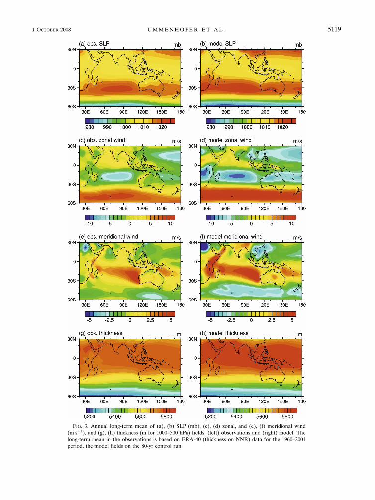
FIG. 3. Annual long-term mean of (a), (b) SLP (mb), (c), (d) zonal, and (e), (f) meridional wind(m s�1), and (g), (h) thickness (m for 1000–500 hPa) fields: (left) observations and (right) model. Thelong-term mean in the observations is based on ERA-40 (thickness on NNR) data for the 1960–2001period, the model fields on the 80-yr control run.


Fig 3 live 4/C

captures the overall Southern Hemisphere patternswith a distinct meridional SLP gradient (Figs. 3a,b).However, the pattern is overly zonally symmetric(across all seasons) in the midlatitudes compared to theobservations (Sen Gupta and England 2006), resultingin an exaggerated meridional SLP gradient (Hurrell etal. 2006). The seasonal cycle in the movement of thesubtropical high pressure belt and the circumpolartrough agrees well with observations, though the latteris too deep and positioned too far equatorward in win-ter (Hurrell et al. 2006). The overall pattern of sub-tropical easterlies and midlatitude westerlies at the sur-face across the Indian Ocean region is captured in themodel (Figs. 3c,d). However, as before, the zonal com-ponent in the model is slightly overestimated, with apositive bias in the midlatitude westerlies for the lati-tude band of 35°–60°S compared to the observations,especially south of Australia and toward New Zealand(Hurrell et al. 2006), and an overly strong easterly windfield across the central Indian Ocean, over northernparts of Australia and extending eastward. In the sub-tropical easterlies this is especially apparent in the win-ter half of the year (figure not shown). The meridionalwind field in the model closely matches the observa-tions (Figs. 3e,f), with only a slightly enhanced north-erly (southerly) component in the latitude band of 40°–60°S (along eastern Africa). The observed seasonalcycle of strengthening southerly winds across much ofthe Indian Ocean during the winter months is also wellrepresented in the model (figure not shown). The me-ridional gradient in thickness is captured very well bythe model, and the differences to the observations aresmall (Figs. 3g,h).

Several biases in the model have been documentedpreviously; most notably, there is a spurious secondITCZ south of the equator in the Pacific and hence apoor simulation of the SPCZ (Zhang and Wang 2006).This is a problem common to many atmospheric gen-eral circulation models (Meehl and Arblaster 1998;Hurrell et al. 2006). The positive bias in the tropicalPacific rainfall in both branches of the ITCZ signifiesan overly vigorous hydrological cycle there (Collins etal. 2006). The double-ITCZ problem has been linked toa bias in SST in the equatorial Pacific region (Arblasteret al. 2002; Zhang and Wang 2006). This relates to thespatial pattern of ENSO in the coupled model extend-ing too far west in the Pacific Ocean and being toonarrowly confined to the equator (Deser et al. 2006). Inthe atmosphere-only mode, these biases are less pro-nounced and Deser et al. (2006) speculate that theycontribute to the ENSO frequency in the coupledmodel being too high (2–2.5 yr; e.g., Collins et al. 2006;Deser et al. 2006) relative to the observed frequencies

(3–8 yr; e.g., Kiehl and Gent 2004; Zelle et al. 2005;Collins et al. 2006). So, for the scope of the presentstudy and considering our focus on Indian Ocean vari-ability, the general structure and variability in the tropi-cal Pacific is sufficiently well captured by the model.

b. Precipitation

In Fig. 4, the model precipitation across the IndianOcean basin is compared to observed estimates basedon CMAP data (Xie and Arkin 1996). Because clima-tologies of observed rainfall differ considerably on bothregional and local scales, differences to the modelshould be taken as qualitative only (Hurrell et al. 2006).The model represents broad patterns of annual meanprecipitation across the Indian Ocean basin well, withincreased rainfall in the tropics and lower rainfall in theregion of the subtropical high pressure belt across theeastern Indian Ocean and over Australia, as well asAfrica (Figs. 4a,b). However, the model shows exces-sive rainfall over the Indonesian Archipelago and theBay of Bengal compared to the observations, becausethe tropical maximum remains north of the equatorthroughout the year (Hurrell et al. 2006). In contrast,the high-rainfall region in the central equatorial IndianOcean receives too little rainfall. The latter discrepancyis associated with the simulation of a double ITCZ, thatis, the persistence of ITCZ-like precipitation north ofthe equator throughout the year (Hack et al. 2006),which is a problem common to many general circula-tion models (e.g., Meehl and Arblaster 1998; Hurrell etal. 2006; Zhang and Wang 2006; Zhang et al. 2007). Thelow-rainfall region in the eastern subtropical IndianOcean is too dry in the model to the west of Australia,while south of 40°S the model is too wet across theentire Indian Ocean basin compared to the observa-tions, related to a positive bias poleward of the extra-tropical storm tracks (Hack et al. 2006). Meehl et al.(2006) assess the seasonally varying rainfall associatedwith monsoonal regimes across the tropical IndianOcean in CCSM3 in detail. They find the major mon-soonal wind features and associated precipitationmaxima to be well simulated in the model. Future workwill explore impacts of the characteristic SST patternused in this study on precipitation across the wider In-dian Ocean region.

Across Australia (Figs. 4c,d) the overall rainfall dis-tribution, with wetter coastal regions especially alongthe northern and eastern coastline, and a very dry in-terior, is simulated well, although the contrast is weakerthan observed. In particular, the increased rainfall inthe tropical north extends too far inland, as can be seenin Fig. 6b of Meehl et al. (2006). Notwithstanding theseshortcomings, the seasonal cycle with the associated


FIG. 4. Annual long-term mean of (a)–(d) rainfall (mm yr�1) fields across (a), (b) the Indian Ocean basin and (c), (d) magnified overthe Australian continent with the (left) observations and (right) model. The long-term mean in the observations in (a) is based onCMAP data for the 1979–2001 period, in (c) on the SILO data for 1960–2001, and in (b) and (d) on the model fields from the 80-yrcontrol run (though for ease of comparison between observed and model, only the first 40 yr of the control are shown). The dashedbox in (c) indicates the area used to derive the (e) observed and (f) model SWWA precipitation time series shown as annual values.The dashed box in (d) depicts the area termed WA. (g) The long-term seasonal cycle in precipitation for the observations (solid) andmodel (dashed). (h) The power spectral density shows the observed (model) variance for the dominant cycles in blue (red), with thedashed lines indicating a 95% confidence level according to white noise.


Fig 4 live 4/C

precipitation regimes across the Australian continent(i.e., winter rainfall in the south, summer monsoonalrainfall in the north) compare very favorably with ob-servations (figure not shown). Despite a few regionalrainfall deficiencies in the model, useful inferences canstill be made regarding mechanisms for change in thesimulations.

The time series for SWWA rainfall in the observa-tions and the model (Figs. 4e,f) were derived for theregion outlined by the boxes in Figs. 4c,d (for detailsalso see section 2d). On average, the SWWA regionrecords 540 mm yr�1 in the observations, while only 360mm yr�1 are received in the model. The lower rainfallin the model is characteristic of climate models, consid-ering its coarser resolution relative to the observations.The standard deviation of 74 mm yr�1 in the observa-tions compares with 48 mm yr�1 in the model. How-ever, a more appropriate metric of variability, the co-efficient of variation (i.e., ratio of standard deviationand mean), demonstrates good agreement, with 0.137and 0.133 for the observations and model, respectively.This indicates a comparable variability in SWWA rain-fall on interannual time scales between observationsand CAM3.

In line with the modeled annual mean precipitation,the amplitude of the seasonal cycle in the total precipi-tation is reduced over a large part of the year (May–November) in the model relative to the observations(Fig. 4g). However, the phase of the seasonal cycle withthe majority of the rainfall falling in May–September iswell reproduced. Model precipitation is given as thecombination of stable large-scale and convective com-ponents. While the SILO dataset does not distinguishbetween these components, they are available as part ofthe NNR and are compared to the model components(figure not shown). For both the model and observa-tions, the contribution of large-scale precipitation isconsiderably less than that resulting from convection.In the observations, convective rainfall occurs predomi-nantly in winter (April–October), while it is moreevenly distributed across the year in the model becauseof overestimated summer levels. The model large-scaleprecipitation in contrast is slightly higher than that ob-served throughout the year, though it reproduces theobserved seasonal cycle of enhanced rainfall duringApril–August. Overall, the model has a higher propor-tion of total rainfall resulting from large-scale precipi-tation. Further investigation into the parameterizationof precipitation in the model for convective and large-scale rainfall, and a detailed comparison with the NNRis beyond the scope of this study. Because broad fea-tures of the relative contribution of the two compo-nents and their seasonal cycle agree between the model

and observations, it seems reasonable to assume thatthe model is sufficiently realistic in terms of SWWAprecipitation to be a useful tool to investigate precipi-tation characteristics. This is further suggested by aspectral analysis of SWWA rainfall showing coincidentpeaks in model and observed time series (Fig. 4h; peaksat 2–3 and 10 yr are significant at the 95% confidencelevel).

4. Seasonal evolution of the SST perturbation

The SST anomalies used in the perturbation experi-ments are based on characteristic observed SST pat-terns identified by England et al. (2006). The monthlyvarying SST anomalies averaged across their anoma-lous dry years in SWWA are shown in Fig. 1. They formthe basis for the PDRY run. England et al. (2006) founda characteristic tripole pattern in Indian Ocean SST [forthe specific location of the poles see Fig. 5 in Englandet al. (2006)], consisting of one pole off the shelf to thenorthwest of Australia extending northwestward toSumatra (P1; centered near 15°S, 120°E), a second poleof opposite polarity in the central subtropical IndianOcean (P2; near 30°S, 100°E), and a third pole of thesame sign as P1 to the southeast of Madagascar (P3;near 40°S, 50°E). In the remainder of the paper we willrefer to those poles as P1, P2, and P3. This patterngradually forms over the course of the year, becomingmost prominent in late winter/early spring. Though notyet fully formed, the cold SST anomalies at P1 appearas early as January. In contrast, the warm anomalies atP2 are briefly revealed during January and February,but then weaken again until in May when they re-emerge and become a persistent feature. The anomaliesin all three poles intensify until October. From Novem-ber onward, anomalies in P1 decline, while the warmSST of P2 extends northward and covers the entire In-dian Ocean north of 30°S by December. The seasonalevolution of the SST perturbation during PWET shows asimilar spatial and temporal development to PDRY, withSST anomalies of opposite polarity (figure not shown).

It is of interest to compare the seasonal evolution ofthe pattern and magnitude of the composite SSTanomalies used in the PDRY simulation (Fig. 1) with theSST anomalies in a particular dry year in SWWA,namely 2006. The SWWA growing season (May–October) in 2006 was the driest ever recorded for manyof the agricultural areas in Western Australia(DAFWA 2006). The SST anomalies of that specificdry year were not incorporated into the PDRY forcingfield, because only extreme years prior to 2003 wereincluded in the England et al. (2006) composites. Theseasonal evolution of SST anomalies in 2006 (Fig. 2)


broadly matches those in Fig. 1, both spatially and tem-porally, and in magnitude. In 2006, the SST anomaliesat P1 and P2 intensified over the course of the yearreaching maximum values of up to �1°C in winter/earlyspring, which is of comparable magnitude to the per-turbations in the same months (up to �1.2°C). Theclose match between the composite SST anomaliesused as forcing and the 2006 SST anomalies demon-strates that the forcing is not of an unrealistically largemagnitude. The use of the composite pattern for theforcing, rather than the pattern of a single year, allowsmore general inferences about other anomalous dry/wet years to be made. Similarly in 2005, a year withabove-average precipitation across SWWA, themonthly SST anomalies across the Indian Ocean closelymirror the PWET SST pattern (figures not shown), bothtemporally and spatially, and with anomalies of a com-parable magnitude. This provides some limited evi-dence that the SST perturbations we apply represent arecurring SST pattern over the Indian Ocean. Correla-tion of the SWWA rainfall and Indian Ocean SST alsoreveals a qualitatively similar pattern with the threepoles apparent (figure not shown). An empirical or-thogonal function analysis of observed Indian OceanSST (not shown) confirms this, with the second mode(the first mode represents the warming of the IndianOcean) explaining 16% of the total variance in SST(Santoso 2005). This is of the same order of magnitudeas the SST variance accounted for by the IOD (12%;Saji et al. 1999). The identification of the effects of thispattern on regional climate conditions is therefore ofconsiderable importance.

As pointed out by England et al. (2006), the locationand evolution of the poles in the Indian Ocean SSTshown here (Figs. 1 and 2) are distinct from previousdefinitions of characteristic SST patterns, some ofwhich have been linked to Australian rainfall. How-ever, some similarities with previous SST patterns existboth in the tropics and subtropics of the Indian Ocean.The evolution of P1 in PDRY is similar to the easternpole of the tropical IOD shown by Saji et al. (1999) intheir Fig. 2, especially in the second half of the year.The subtropical Indian Ocean dipole (SIOD) of Beheraand Yamagata (2001) in their Fig. 4 is displaced to thewest relative to our poles, with their warm SST anoma-lies located over the western edge of P2 and overlap-ping P3, and their cold pole to the west of P1 and lessclearly defined. In addition, their SIOD SST anomaliesreach their maximum earlier in the year (around Feb-ruary/March) compared to July–October in this study.The broad features of SST anomalies associated withthe first rotated principal component of Australian an-

nual precipitation in Fig. 3 in Nicholls (1989) broadlyagree with our PDRY perturbation pattern (Fig. 1),though most closely during the August–October pe-riod. In light of the distinctiveness of our SST patternsfrom previous studies, both spatially and temporally,and their link to SWWA rainfall (England et al. 2006),it is of interest to explore the precipitation anomaliesacross western regions of Australia induced by theseSST perturbations in an AGCM.

5. Precipitation changes

a. SWWA

We first assess the impact of the changed SST fieldsin the perturbation experiments on the rainfall distri-bution in the more limited SWWA region (Fig. 4c). Themodel rainfall distributions over SWWA across the en-semble members in PDRY and PWET relative to CNTRLare shown in Figs. 5 and 6, summed over differentmonths. The model separates large-scale and convec-tive precipitation, providing a first indication of likelycauses in any shift in the rainfall distribution (based onall months) between PDRY and PWET. The large-scaleannual rainfall distribution is shifted toward low (high)rainfall amounts for PDRY (PWET) relative to the CNTRL(both are significant at the 99% confidence level; seeFigs. 5a,b). This is especially apparent at the upper endof the rainfall distribution for years receiving in excessof 150 mm yr�1: while in the CNTRL case 8% of theyears receive 150–170 mm yr�1, none of the years inPDRY record more than 150 mm yr�1, but in 25% of theyears in PWET this threshold is passed (annual rainfallof 150–170 mm yr�1 occurring in 13% of the years,70–190 mm yr�1 in 7%, and 190–210 mm yr�1 in 5%).When focusing on the main rainfall season for SWWA,the period (May–September) during which 70% of theannual rainfall occurs, the same trends are observed,namely, a significant reduction (increase) is seen in thenumber of ensemble members receiving in excess of100 mm of rainfall during May–September for the PDRY

(PWET) case (Figs. 5c,d). For austral winter (June–August; Figs. 5e,f), only 5% of winters in the PDRY casereceive more than 65 mm, while this occurs in 9% ofwinters in the CNTRL and 32% in the PWET case.Overall, a consistent shift in the large-scale annual andseasonal rainfall distribution is observed, with the up-per end of the distribution losing (gaining) a dispropor-tionate number of events for the dry (wet) cases.

The frequency distribution for convective rainfallover SWWA shows less consistent shifts (Fig. 6), withan apparent asymmetry between PDRY and PWET. Anincrease in the number of years with high convective


precipitation is observed for the PDRY case (Figs.6a,c,e). This trend is significant at the 99% confidencelevel for the January–December, May–September, andJune–August periods. In contrast, the convective rain-fall distribution for PWET does not differ significantlyfrom the CNTRL. A mechanism explaining this asym-metry, whereby the PDRY forcing actually induces anincrease in convective rainfall, will be proposed in sec-tion 6.

b. Western Australia

We focus now on a larger area across WA, excludingthe tropical north of the state (see Fig. 4d). For this

larger region, shifts in rainfall distribution are evidentfor both the large-scale and convective precipitationand are of the same sign. Figure 7 presents the fre-quency distribution of total rainfall for WA. Now, theentire frequency distribution pattern for the annual to-tal rainfall is clearly shifted toward lower (higher) rain-fall amounts in the PDRY (PWET) case relative to theCNTRL (significant at the 99% confidence level; Figs.7a,b). The shifts for the May–September and June–August are less prominent, though still significant asindicated (Figs. 7c–f). This can be attributed to the factthat as we extend the investigated area farther inland,we move from a region with predominant winter pre-

FIG. 5. Frequency distribution of large-scale rainfall spatiallyaveraged across SWWA: rainfall amount (mm) summed for themonths of (top) January–December, (middle) May–September,and (bottom) June–August for (left) PDRY and (right) PWET cases.The shaded gray rainfall distribution represents the CNTRL (nor-malized to the number of ensemble members in PDRY/PWET),while PDRY and PWET are indicated with black outlines. The fol-lowing significance levels hold, as determined by a Mann–Whitney test: (a) 99%, (b) 99%, (c) 99%, (d) 95%, (e) 90%, and(f) 95%.

FIG. 6. Frequency distribution of convective rainfall spatiallyaveraged across SWWA: rainfall amount (mm) summed for themonths of (top) January–December, (middle) May–September,and (bottom) June–August for (left) PDRY and (right) PWET cases.The shaded gray rainfall distribution represents the CNTRL (nor-malized to the number of ensemble members in PDRY/PWET),while PDRY and PWET are indicated with black outlines. The fol-lowing significance levels hold, as determined by a Mann–Whitney test (if nothing indicated, below 80%): (a) 99%, (c) 99%,(d) 80%, and (e) 99%.


cipitation toward a more uniform distribution through-out the year. This means that the prominent shifts inannual rainfall distribution (Figs. 7a,b) are accumulatedover the whole year. Furthermore, the opposing trendsin convective and large-scale precipitation seen inSWWA are not apparent for the larger region WA.This relates most likely to the fact that with increasingdistance inland, the impact of the warm SST at P2,giving rise to localized convective upward motionand enhanced convective rainfall in SWWA duringPDRY, is averaged away. The asymmetry in the convec-tive rainfall over SWWA, not seen in the analysis forWA, will be investigated in more detail in section 6,

when the atmospheric dynamics leading to the changedrainfall distribution are explored.

c. Seasonal variability

The seasonal cycle in SWWA and WA rainfall in theperturbed cases is further investigated for the differentrainfall types. The total monthly large-scale rainfallover each region is presented in Fig. 8, showing a no-table reduction (increase) in PDRY (PWET). In contrast,when including convective events, the total rainfall (fig-ure not shown) in PDRY shows an intensification of theseasonal cycle with enhanced winter precipitation(May–August) and a reduction in autumn, relative tothe CNTRL. This amplification of the seasonal cycle inPDRY can be attributed to the positive (negative)changes in the convective winter (autumn) rainfall,

FIG. 7. Frequency distribution of total rainfall spatially aver-aged across Western Australia: rainfall amount (mm) summed forthe months of (top) January–December, (middle) May–September, and (bottom) June–August for (left) PDRY and (right)PWET cases. The shaded gray rainfall distribution represents theCNTRL (normalized to the number of ensemble members inPDRY/PWET), while PDRY and PWET are indicated with black out-lines. The following significance levels hold, as determined by aMann–Whitney test: (a) 99%, (b) 99%, (c) 95%, (d) 99%, (e)90%, and (f) 99%.

FIG. 8. Long-term seasonal cycle in model large-scale precipi-tation in the CNTRL (black), PDRY (red), and PWET (blue) runsover (a) SWWA and (b) Western Australia.


Fig 8 live 4/C

while the annual cycle in large-scale rainfall remainsunchanged. In contrast, PWET is characterized byslightly wetter conditions in both rainfall types through-out the year, particularly in summer and autumn. So, inthe PDRY case, a further enhancement of the predomi-nant winter precipitation occurs, driven largely by anincrease in convective rainfall, while the amplitude ofthe seasonal cycle in PWET rainfall is reduced. Asabove, the seasonal cycle of SWWA large-scale pre-cipitation in the perturbed cases overall follows theCNTRL (Fig. 8a), though with a notable reduction(increase) in PDRY (PWET). For WA, although the sea-sonal cycle for large-scale precipitation also re-mains unchanged in the perturbed cases relative to theCNTRL, the rainfall amounts in each month deviateconsiderably more from the CNTRL than for thesmaller region of SWWA. That is, in all months prior toNovember the large-scale precipitation in PDRY (PWET)consistently lies below (above) the CNTRL fields (Fig.8b).

6. Mechanisms and atmospheric dynamics

To understand the mechanism responsible for the ob-served local and regional rainfall changes we now in-vestigate large-scale atmospheric anomalies. Both ther-mal properties and circulation characteristics are ex-plored across the Indian Ocean and adjacentlandmasses during the dry and wet ensemble of experi-ments.

a. Thermal anomalies in the atmosphere

The seasonal thickness anomalies in Fig. 9 provide ameasure of the thermal properties in the lower atmo-sphere and resultant atmospheric flow. The seasonalevolution of the PDRY thickness anomalies (Figs. 9a,c,e)follows the evolution of the underlying SST anomalies(Fig. 1). In concert with the cold SST anomalies, nega-tive thickness anomalies occur over the eastern IndianOcean, south of Australia, and across parts of Australiaduring the first 3 months of the year. Warm SSTanomalies in the central subtropical Indian Ocean startestablishing the characteristic dipole pattern (P1 andP2) from May onward (Fig. 9; although individualmonths are not shown). This is followed by the forma-tion of a positive thickness anomaly extending from thecentral subtropical Indian Ocean across southern re-gions of Australia, including SWWA, from July on-ward. During the winter months until October, the pat-tern of negative, positive, and negative thicknessanomalies across the Indian Ocean (extending from the

northeast toward the southwest), reflects the sign andpositions of P1, P2, and P3 in SST anomalies, respec-tively. The combination of the three poles leads to aneasterly anomaly in the thermal wind across theSWWA region. This would lead to a weakening of thesubtropical jet that normally reaches peak strength dur-ing the winter months, resulting in weaker interactionswith low pressure disturbances and cold fronts movingthrough the region. This could account for the reduc-tion in large-scale rainfall during PDRY and is particu-larly prominent during the winter months (Figs. 5c,e).The positive thickness anomaly over SWWA persistsuntil October.

The development of the thickness anomalies duringPWET over the eastern Indian Ocean and Australia(Figs. 9b,d,f) is, on a broad scale, the reversal of thePDRY evolution. Positive thickness anomalies dominateuntil April across the Indian Ocean region and Austra-lia. Simultaneous with a strengthening of the PWET SSTdipole structure in May (figure not shown), warm thick-ness anomalies strengthen over the P1 location to thenorthwest of Australia. At the same time, cold thick-ness anomalies develop in the subtropical Indian Oceanoff the coast of SWWA. The meridional gradient inthickness between the tropics (P1) and subtropics (P2)further intensifies over the following months. This rep-resents an intensification of the underlying seasonalcycle. The intersecting line between positive and nega-tive anomalies to the north and south, respectively,passes through SWWA, extending toward the south-east. It moves farther north in September, with negativeanomalies covering all southern regions of Australia.

The monthly thickness anomalies in both PDRY andPWET show the greatest response in the May–September period when the majority (close to 75%) ofthe annual SWWA precipitation falls. Hence, for theremainder of this study, we will focus on the May–September months. The thermal structure through theatmosphere arising from the SST perturbations isshown in cross-sections at 32°S in Fig. 10 averaged overthe May–September period. The characteristic struc-ture of cold (warm) SST anomalies at P1, warm (cold)anomalies at P2, and cold (warm) anomalies at P3 forPDRY (PWET) is apparent (Figs. 10a,b). The location ofthe cross section at 32°S is indicated by the black line inFigs. 10a,b and directly traverses the center of P2, whilealso showing some influences of P3. The warm tem-perature anomalies at P2 in PDRY penetrate to a heightof more than 4 km (Fig. 10c), with the maximum in-creases in temperature below 2 km (about 800 hPa). Incontrast, the cold anomalies at P2 in PWET only reach toa height of 2 km and are capped by warm anomalies


aloft (Fig. 10d). This asymmetry seems reasonable, be-cause warm surface anomalies will produce a more un-stable air column that has the ability to mix the warmair higher into the atmosphere than the cold anomalies.This may explain the increase in convective rainfallover SWWA seen in PDRY (Fig. 6c), but not in PWET

(Fig. 6d), because the convective activity in the formerwould be stronger likely because of the enhanced tem-perature lapse rate through a deep atmospheric col-umn. By way of contrast, the thermal structure in Fig.10d seems more favorable for episodes of slow wide-spread ascent and associated rain, as warm, moist air isforced to move southward over the cold SST anomalyby an eastward-moving trough. The asymmetry mayadditionally affect circulation anomalies arising from

changes in the thermal properties of the atmosphere.This is investigated below.

b. Circulation anomalies in the atmosphere

Circulation anomalies in the atmosphere are shownin Fig. 11 for horizontal winds at 500 hPa and verticalvelocity at 700 hPa during the May–September periodfor PDRY and PWET, respectively. Broadly speaking,anomalies in the horizontal winds relate to changes inthe large-scale stable precipitation, while vertical veloc-ity anomalies mostly are associated with convectiverainfall. During PDRY, there is a weakening of the an-ticyclonic circulation over the Indian Ocean basin (Fig.11a). This is especially apparent in a reduction in the

FIG. 9. Average seasonal thickness (m, for 1000–500 hPa) anomaly for (left) PDRY and (right) PWET, relative to the CNTRL for the(a), (b) March–May, (c), (d) June–August, and (e), (f) September–November seasons. Dashed lines indicate significant anomalies atthe 90% confidence level as estimated by a two-tailed t test.


Fig 9 live 4/C

easterly wind field over the eastern Indian Ocean at10°–20°S. Over southern regions of Australia, easterlyanomalies occur as well, resulting in anomalous off-shore flow over SWWA. In contrast during PWET, en-hanced onshore flow and westerly anomalies dominateover the Australian continent south of 20°S (Fig. 11b).The weakened (strengthened) onshore wind anomaliesare consistent with the sign and position of the reduced(enhanced) gradient in thickness resulting from the un-derlying cold (warm) SST anomalies at P1 and warm(cold) anomalies at P2 during PDRY (PWET). The sur-face horizontal circulation anomalies induced by theSST perturbations in this study (figure not shown)closely mirror anomalous surface winds associated withdry/wet SWWA rainfall years in observations (Englandet al. 2006).

Significant anomalies in vertical velocity (Figs. 11c,d)are mainly confined to the tropics, being positive (nega-tive) over the equatorial eastern Indian Ocean andparts of the Indonesian Archipelago during PDRY

(PWET). This reduction (enhancement) in rising motionover the equatorial Indian Ocean during PDRY (PWET)is located above the underlying cold (warm) SSTanomalies at P1. Significant vertical velocity anomalies

over the P2 pole occur in the PDRY case only. Thisindicates a reduction in subsidence off the SWWAcoast (Fig. 11c). Again, this helps to explain the signif-icant increase in convective rainfall over SWWA forPDRY (Fig. 6c), but not for PWET (Fig. 6d).

A further indication of stability in the atmosphere isprovided by the Eady growth rate, a measure of thebaroclinic instability in the atmosphere. The Eadygrowth rate was calculated according to Paciorek et al.(2002), using the vertical gradient in horizontal windspeed and the Brunt–Väisälla frequency as a measureof static stability. It provides an indication of the de-velopment of low pressure systems (Risbey et al. 2007,manuscript submitted to Int. J. Climatol.), which areassociated with increased rainfall. Mean states of theEady growth rate in the model during winter (figure notshown) compare well with observations (e.g., Fig. 5 inRisbey et al. 2007, manuscript submitted to Int. J. Cli-matol.). During the May–September period in PDRY,negative anomalies in Eady growth rate extendingacross southern regions of Australia indicate a reduc-tion in baroclinicity and hence a lower formation rate ofinstabilities (Fig. 12a). An increase in instabilities isseen over northern regions of Australia and the eastern

FIG. 10. (a), (b) SST perturbation and (c), (d) cross section of air temperature anomalies for the (left) PDRY and(right) PWET case averaged over the May–September period (°C). The 32°S location of the cross section in (c), (d)is marked by black lines in (a), (b). Dashed lines in (c), (d) indicate significant anomalies at the 90% confidencelevel as estimated by a two-tailed t test.


Fig 10 live 4/C

FIG. 11. Anomalies of (a), (b) winds at 500 hPa (m s�1) and (c), (d) vertical velocity at 700 hPa (Pa s�1) for the (left) PDRY and (right)PWET case averaged over the May–September period (positive, being downward). Black vectors in (a), (b) and dashed lines in (c), (d)indicate significant anomalies at the 90% confidence level as estimated by a two-tailed t test.

FIG. 12. Anomalies of Eady growth rate (day�1) for the (a) PDRY and (b) PWET case averaged over the May–September period.Dashed lines indicate significant anomalies at the 90% confidence level as estimated by a two-tailed t test. Positive (negative) valuesindicate an increase (decrease) in baroclinicity and development of more (less) instabilities.


Fig 11 and 12 live 4/C

Indian Ocean over the 10°–20°S latitude band, coincid-ing with the westerly wind anomalies there (Fig. 11a).The positive anomalies in Eady growth rate duringPWET are centered over SWWA and the adjacent In-dian Ocean region, representing a local enhancementof baroclinicity with increased instabilities just offshoreof SWWA (Fig. 12b). The location of the increasedbaroclinicity over the P2 cold SST anomalies duringPWET hints at their role in forcing the increased large-scale rainfall recorded over SWWA. In contrast, re-duced instability is observed overlying the P1 region offthe northwest shelf of Australia. Under an enhancedSST gradient in the eastern Indian Ocean reminiscentof the PWET forcing, Frederiksen and Frederiksen(1996) find increased baroclinicity and an equatorwardshift of storm-track instability modes over southern re-gions of Australia. This is consistent with the resultspresented here.

7. Summary and conclusions

In this study we have used AGCM simulations toassess the way Indian Ocean SST anomalies modulatemidlatitude precipitation across southern and westernregions of Australia. This represents an extension ofprevious work by England et al. (2006) who find ex-tremes in SWWA rainfall associated with characteristicSST patterns and reorganization in the large-scale at-mospheric circulation across the Indian Ocean. Here,we have presented evidence that these composite SSTpatterns significantly affect SWWA and WA precipita-tion in ensemble sets of AGCM simulations. We havealso proposed a mechanism for the observed rainfallshifts resulting from changes in the large-scale generalcirculation.

Good agreement between the model mean fields andreanalysis data on annual and seasonal time scales in-dicates that the model represents the general atmo-spheric circulation across the Indian Ocean region suit-ably well. Over the Australian continent, the seasonalrainfall distribution associated with the monsoons inthe north in summer and winter rainfall in the south ofthe country are well captured, though some regionalbiases exist (e.g., Meehl et al. 2006). Over the studyregion of SWWA, interannual variability and the sea-sonal cycle of the observed and model rainfall is com-parable, although the long-term means in the model arelower than those observed. Despite certain biases in themodel regarding tropical Pacific climate (e.g., Zhangand Wang 2006; Deser et al. 2006) and a slight enhance-ment of zonal flow at midlatitudes (Sen Gupta and

England 2006; Hurrell et al. 2006), the model performssufficiently well over the Indian Ocean and Australianregion to justify its use in the present study.

The monthly varying Indian Ocean SST compositepatterns used as perturbations in the AGCM simula-tions appear to represent a realistic and recurring SSTpattern (Santoso 2005). This is evidenced by the closematch in the spatial and temporal evolution of the dry-year SST perturbation (Fig. 1) and the SST anomaliesduring 2006, which are not included in the compositefields (Fig. 2). The characteristic dipole pattern, whichis distinct in location and temporal evolution from pre-vious definitions of dipoles in the Indian Ocean (e.g.,Saji et al. 1999; Behera and Yamagata 2001), developswith cold (warm) SST anomalies in the eastern IndianOcean over the northwest shelf of Australia (P1) andwarm (cold) anomalies in the central subtropical IndianOcean (P2) during dry (wet) years in SWWA, reachingmaximum values in late winter/early spring (Fig. 1).

Significant changes occur in the distribution ofSWWA and WA precipitation in the perturbation ex-periments with the modified SST patterns (PDRY andPWET). In particular,

1) A consistent shift in winter and annual large-scalestable precipitation over SWWA is recorded, withthe upper end of the distribution losing (gaining) adisproportionate number of events in PDRY (PWET).

2) An apparent asymmetry is seen in the response ofwinter and annual convective precipitation inSWWA, with an increase in PDRY convective rain-fall, while no significant changes are apparent inPWET.

3) For WA, a shift of the entire rainfall distributiontoward the low (high) end of the distribution is ob-served for PDRY (PWET), for both convective andlarge-scale precipitation.

To understand the mechanism(s) responsible forthese rainfall changes, we investigated anomalies inthermal properties of the atmosphere and in the gen-eral circulation. Thickness anomalies of the same signand position as the underlying SST anomalies at P1 andP2 develop in the perturbation experiments, intensify-ing toward late winter and extending across southernregions of Australia (Fig. 9). This leads to a weakening(intensification) of the meridional thickness gradientand the subtropical jet during the winter in PDRY

(PWET), with a coincident easterly (westerly) anomalyin the thermal wind over southern regions of Australia.The anomalously offshore (onshore) winds overSWWA (Figs. 11a,b) could thus contribute to a reduc-


tion (increase) in large-scale rainfall. In the observedrecord, Ansell et al. (2000) similarly associate variations(and trends) in SWWA rainfall with modulations in thesubtropical high pressure belt and a shift of the circum-polar trough. However in their study, links with Indianand Pacific Ocean SST are weak compared to the vari-ability of the large-scale atmospheric circulation, whilewe demonstrate that the reorganization in the generalatmospheric circulation arises as a result of the changedSST fields in the AGCM simulations.

A measure of the baroclinic stability in the atmo-sphere, and hence its disposition toward the develop-ment of rain-bearing low pressure systems, is providedby the Eady growth rate (Paciorek et al. 2002). A re-duction (increase) in the Eady growth rate (Fig. 12)indicates a lower (higher) formation rate of baroclinicinstabilities over southern and western regions of Aus-tralia during PDRY (PWET), consistent with the large-scale rainfall changes. Hope et al. (2006) also linkedtrends in baroclinicity and reduced frequency of passingtroughs across the region with the observed rainfall de-crease in SWWA. Similarly, Frederiksen and Frederik-sen (2005, 2007) suggest that these decreases resultedfrom changes in the intensity and southward deflectionof regions of cyclogenesis resulting from a decline inmidlatitude baroclinicity. Over the Australian region,they find a 30% decrease in the growth rate of leadingSouthern Hemisphere cyclogenesis modes associatedwith a reduction in the vertical mean meridional tem-perature gradient, and in the peak upper-troposphericjet stream zonal winds at 30°S. Here, we have demon-strated that such changes can be forced by anomalousSST patterns over the Indian Ocean.

The asymmetry in convective precipitation can berelated to anomalies in the thermal properties of theatmosphere (Fig. 10), with the warm underlying SST atP2 during PDRY penetrating higher into the atmosphere(resulting from an enhanced temperature lapse rate)than the cold PWET anomalies. The vertical thermalstructure in PDRY thus could favor localized increases inconvective activity, as seen in the increase in convectiverainfall over SWWA and the reduction in large-scalerainfall. On the other hand, both the circulation andthermal anomalies in PWET may enhance widespreadascent of moist air masses associated with frontal move-ment, as evidenced by increases in large-scale precipi-tation in that ensemble set.

Considering the significant drop in precipitation inSWWA since the 1970s (e.g., Allan and Haylock 1993;IOCI 2001; Timbal et al. 2006) and the projections forits continuation over the coming decades (Cai et al.2003; Timbal 2004; Cai and Cowan 2006; Hope 2006), it

is of interest to relate our findings on interannual rain-fall variations in SWWA to long-term trends. Recentchanges in the large-scale Southern Hemisphere gen-eral circulation have been described in several studies.These include trends in the SAM toward its high-indexphase (e.g., Li et al. 2005; Cai and Cowan 2006; Hendonet al. 2007), a consistent poleward shift in the zones ofstrong baroclinicity (Yin 2005), reductions in the den-sity of low pressure systems (Smith et al. 2000), shifts inthe subtropical jet (Frederiksen and Frederiksen 2005),and the reduced intensity of cyclogenesis (Frederiksenand Frederiksen 2005, 2007), among others. In thisstudy, we have identified mechanisms by which thesefactors, driven by SST, modulate precipitation, both ata regional scale for SWWA and over interannual timescales. It is thus possible that the ocean plays a vital rolein driving these atmospheric circulation changes thathave led to longer-term trends in SWWA rainfall, es-pecially as recent Indian Ocean SST trends favor a ten-dency toward the PDRY thermal gradient (England etal. 2006). This is supported by other studies. For ex-ample, Smith et al. (2000) suggest that long-termSWWA rainfall variability is influenced by coupled air–sea interactions across the South Indian Ocean, linkingSST and MSLP. Frederiksen and Balgovind (1994)demonstrated a connection between the frequency ofnorthwest cloud bands and Indian Ocean SST gradi-ents.

In summary, we have presented evidence that IndianOcean SST is indeed instrumental in forcing midlati-tude rainfall changes over regions of southern and west-ern Australia. The characteristic SST pattern we inves-tigate is thus not simply symptomatic of the changedwind field, but it could also play an important role inmodulating the atmospheric circulation and rainfallanomalies. These findings are in contrast with someprevious work on midlatitude rainfall in general (Kush-nir et al. 2002, and references therein), and for the Aus-tralian region in particular (Watterson 2001, though hisexperiments do not employ a scaled SST forcing). Wedo not dispute the main hypothesis of Watterson(2001)—that interannual variations in seasonal rainfallare primarily driven by internal atmospheric mecha-nisms. However, this does not rule out the possibility ofsignificant modulation by Indian Ocean SST forcing.Indeed Watterson (2001) refers to other GCM studiesthat find a proportion of the rainfall variance beingexplained by SST variability. Our results suggest amodest, yet significant, change in the frequency distri-bution for rainfall (i.e., the extreme events) resultingfrom SST anomalies, which is not necessarily capturedby a total rainfall metric. It still remains an open ques-


tion as to what initially drives the formation of the char-acteristic SST anomaly pattern (e.g., internal ocean dy-namics, ocean–atmosphere coupling), but this is beyondthe scope of the present study and will be exploredelsewhere. In a separate study, we will further investi-gate the implications of the present findings on improv-ing predictability of SWWA rainfall. Considering thelonger persistence of temperature anomalies in theocean, as opposed to the higher-frequency variability inthe atmosphere, we are hopeful that the mechanismpresented here can help improve seasonal rainfall pre-dictions, and thus ultimately aid in water managementdecisions in SWWA. In addition, the relative influenceof the individual SST poles and the lead time of pre-dictability warrant further investigation; these will beexplored separately in a future study.

Acknowledgments. Use of the NCAR’s CCSM3model is gratefully acknowledged. The CMAP precipi-tation, NNR data, and NOAA_ERSST_V2 SST datawere provided by NOAA/OAR/ESRL PSD, Boulder,Colorado, through their Web site (online at http://www.cdc.noaa.gov), and the ERA-40 data were provided bythe ECMWF. The model simulations were run at theAustralian Partnership for Advanced Computing Na-tional Facility. The manuscript benefitted from helpfuldiscussions with Peter McIntosh and James Risbey, andcomments by three anonymous reviewers. CCU wassupported by the University of New South Wales undera University International Postgraduate Award, ASGand MHE by the Australian Research Council, andMJP partially by the Managing Climate Variability Pro-gram of Land and Water, Australia, and the CSIROWealth from Oceans National Research Flagship.

REFERENCES

Allan, R. J., and M. R. Haylock, 1993: Circulation features asso-ciated with the winter rainfall decrease in Southwestern Aus-tralia. J. Climate, 6, 1356–1367.

Ansell, T. J., C. J. C. Reason, I. N. Smith, and K. Keay, 2000:Evidence for decadal variability in southern Australian rain-fall and relationships with regional pressure and sea surfacetemperature. Int. J. Climatol., 20, 1113–1129.

Arblaster, J. M., G. A. Meehl, and A. M. Moore, 2002: Interde-cadal modulation of Australian rainfall. Climate Dyn., 18,519–531.

Ashok, K., Z. Guan, and T. Yamagata, 2003: Influence of theIndian Ocean Dipole on the Australian winter rainfall. Geo-phys. Res. Lett., 30, 1821, doi:10.1029/2003GL017926.

Behera, S. K., and T. Yamagata, 2001: Subtropical SST dipoleevents in the southern Indian Ocean. Geophys. Res. Lett., 28,327–330.

Cai, W., and T. Cowan, 2006: SAM and regional rainfall in IPCCAR4 models: Can anthropogenic forcing account for south-west Western Australian winter rainfall reduction? Geophys.Res. Lett., 33, L24708, doi:10.1029/2006GL028037.

——, P. H. Whetton, and D. J. Karoly, 2003: The response of theAntarctic Oscillation to increasing and stabilized atmosphericCO2. J. Climate, 16, 1525–1538.

Collins, W. D., and Coauthors, 2006: The Community ClimateSystem Model version 3 (CCSM3). J. Climate, 19, 2122–2143.

Czaja, A., and C. Frankignoul, 1999: Influence of the North At-lantic SST on the atmospheric circulation. Geophys. Res.Lett., 26, 2969–2972.

DAFWA, 2006: Seasonal update, November 2006. Department ofAgriculture and Food, Government of Western Australia, 10pp. [Available online at http://www.agric.wa.gov.au/content/lwe/cli/seasonalupdatenov06.pdf.]

Deser, C., A. Capotondi, R. Saravanan, and A. S. Phillips, 2006:Tropical Pacific and Atlantic climate variability in CCSM3. J.Climate, 19, 2451–2481.

Drosdowsky, W., 1993: An analysis of Australian seasonal rainfallanomalies: 1950–1987. I: Spatial patterns. Int. J. Climatol., 13,1–30.

England, M. H., C. C. Ummenhofer, and A. Santoso, 2006: Inter-annual rainfall extremes over southwest Western Australialinked to Indian Ocean climate variability. J. Climate, 19,1948–1969.

Frederiksen, C. S., and R. C. Balgovind, 1994: The influence ofthe Indian Ocean/Indonesian SST gradient on the Australianwinter rainfall and circulation in an atmospheric GCM.Quart. J. Roy. Meteor. Soc., 120, 923–952.

——, and J. S. Frederiksen, 1996: A theoretical model of Austra-lian Northwest cloudband disturbances and Southern Hemi-sphere storm tracks: The role of SST anomalies. J. Atmos.Sci., 53, 1410–1432.

——, and ——, 2005: Mid-1970s changes in the Southern Hemi-sphere winter circulation. Indian Ocean Climate InitiativeStage 2: Report of Phase I Activity, Indian Ocean ClimateInitiative, 7–11.

——, D. P. Rowell, R. C. Balgovind, and C. K. Folland, 1999:Multidecadal simulations of Australian rainfall variability:The role of SSTs. J. Climate, 12, 357–379.

Frederiksen, J. S., and C. S. Frederiksen, 2005: Decadal changes inSouthern Hemisphere winter cyclogenesis. CSIRO Marineand Atmospheric Research Paper 002, 35 pp.

——, and ——, 2007: Interdecadal changes in Southern Hemi-sphere winter storm track modes. Tellus, 59A, 599–617.

Gentilli, J., 1972: Australian Climate Patterns. Thomas Nelson, 285pp.

Hack, J. J., J. M. Caron, S. M. Yeager, K. W. Oleson, M. M. Hol-land, J. E. Truesdale, and P. J. Rasch, 2006: Simulation of theglobal hydrological cycle in the CCSM Community Atmo-sphere Model Version 3 (CAM3): Mean features. J. Climate,19, 2199–2221.

Harzallah, A., and R. Sadourny, 1995: Internal versus SST-forcedatmospheric variability as simulated by an atmospheric gen-eral circulation model. J. Climate, 8, 474–495.

Hendon, H. H., D. W. J. Thompson, and M. C. Wheeler, 2007:Australian rainfall and surface temperature variations asso-


ciated with the Southern Hemisphere Annular Mode. J. Cli-mate, 20, 2452–2467.

Hope, P. K., 2006: Projected future changes in synoptic systemsinfluencing southwest Western Australia. Climate Dyn., 26,765–780.

——, W. Drosdowsky, and N. Nicholls, 2006: Shifts in the synopticsystems influencing southwest Western Australia. ClimateDyn., 26, 751–764.

Hurrell, J. W., J. J. Hack, A. S. Phillips, J. Caron, and J. Yin, 2006:The dynamical simulation of the Community AtmosphereModel version 3 (CAM3). J. Climate, 19, 2162–2183.

IOCI, 2001: Second research report—Towards an understandingof climate variability in south western Australia. SecondResearch Phase of the Indian Ocean Climate Initiative,204 pp.

Jeffrey, S. J., J. O. Carter, K. B. Moodie, and A. R. Beswick, 2001:Using spatial interpolation to construct a comprehensive ar-chive of Australian climate data. Environ. Model. Softw., 16,309–330.

Kalnay, E., and Coauthors, 1996: The NCEP/NCAR 40-Year Re-analysis Project. Bull. Amer. Meteor. Soc., 77, 437–471.

Kiehl, J. T., and P. R. Gent, 2004: The Community Climate Sys-tem Model, version 2. J. Climate, 17, 3666–3682.

Kistler, R., and Coauthors, 2001: The NCEP–NCAR 50-Year Re-analysis: Monthly means CD-ROM and documentation. Bull.Amer. Meteor. Soc., 82, 247–267.

Kushnir, Y., W. A. Robinson, I. Blad, N. M. J. Hall, S. Peng, andR. Sutton, 2002: Atmospheric GCM response to extratropicalSST anomalies: Synthesis and evaluation. J. Climate, 15,2233–2256.

Li, Y., 2007: Changes of winter extreme rainfall over SouthwestWestern Australia and the linkage to the Southern AnnularMode. Proc. 10th Int. Meeting on Statistical Climatology,Beijing, China, Chinese Academy of Sciences, 15–16.

——, W. Cai, and E. P. Campbell, 2005: Statistical modeling ofextreme rainfall in southwest Western Australia. J. Climate,18, 852–863.

McIntosh, P. C., M. J. Pook, J. S. Risbey, S. N. Lisson, and M.Rebbeck, 2007: Seasonal climate forecasts for agriculture:Towards better understanding and value. Field Crops Res.,104, 130–138, doi:10.1016/j.fcr.2007.03.019.

Meehl, G. A., and J. M. Arblaster, 1998: The Asian–Australianmonsoon and El Niño–Southern Oscillation in the NCARClimate System Model. J. Climate, 11, 1356–1385.

——, ——, D. M. Lawrence, A. Seth, E. K. Schneider, B. P. Kirt-man, and D. Min, 2006: Monsoon regimes in the CCSM3. J.Climate, 19, 2482–2495.

Nagarajan, B., and A. R. Aiyyer, 2004: Performance of theECMWF operational analyses over the tropical IndianOcean. Mon. Wea. Rev., 132, 2275–2282.

Nicholls, N., 1989: Sea surface temperatures and Australian win-ter rainfall. J. Climate, 2, 965–973.

Paciorek, C. S., J. S. Risbey, V. Ventura, and R. D. Rosen, 2002:Multiple indices of Northern Hemisphere cyclone activity,winters 1949–99. J. Climate, 15, 1573–1590.

Pitman, A. J., G. T. Narisma, R. A. Pielke Sr., and N. J. Holbrook,2004: Impact of land cover change on the climate of south-

west Western Australia. J. Geophys. Res., 109, D18109,doi:10.1029/2003JD004347.

Priestley, C. H. B., and A. J. Troup, 1966: Droughts and wet pe-riods and their association with SST. Aust. J. Sci., 29, 56–57.

Rayner, N. A., D. E. Parker, E. B. Horton, C. K. Folland, L. V.Alexander, D. P. Rowell, E. C. Kent, and A. Kaplan, 2003:Global analyses of sea surface temperature, sea ice, and nightmarine air temperature since the late nineteenth century. J.Geophys. Res., 108, 4407, doi:10.1029/2002JD002670.

Rodwell, M. J., D. P. Rowell, and C. K. Folland, 1999: Oceanicforcing of the wintertime North Atlantic Oscillation and Eu-ropean climate. Nature, 398, 320–323.

Rowell, D. P., 1998: Assessing potential seasonal predictabilitywith an ensemble of multidecadal GCM simulations. J. Cli-mate, 11, 109–120.

Saji, N. H., B. N. Goswami, P. N. Vinayachandran, and T. Yama-gata, 1999: A dipole mode in the tropical Indian Ocean. Na-ture, 401, 360–363.

Santoso, A., 2005: Evolution of climate anomalies and variabilityof Southern Ocean water masses on interannual to centennialtimescales. Ph.D. thesis, University of New South Wales, 326pp.

Sen Gupta, A., and M. H. England, 2006: Coupled ocean–atmosphere–ice response to variations in the Southern An-nular Mode. J. Climate, 19, 4457–4486.

Smith, I. N., P. McIntosh, T. J. Ansell, C. J. C. Reason, and K.McInnes, 2000: Southwest western Australian winter rainfalland its association with Indian Ocean climate variability. Int.J. Climatol., 20, 1913–1930.

Smith, T., and R. Reynolds, 2003: Extended reconstruction ofglobal sea surface temperatures based on COADS data(1854–1997). J. Climate, 16, 1495–1510.

——, and ——, 2004: Improved extended reconstruction of SST(1854–1997). J. Climate, 17, 2466–2477.

Sterl, A., and W. Hazeleger, 2005: The relative roles of tropicaland extratropical forcing on atmospheric variability. Geo-phys. Res. Lett., 32, L18716, doi:10.1029/2005GL023757.

Streten, N. A., 1981: Southern Hemisphere sea surface tempera-ture variability and apparent associations with Australianrainfall. J. Geophys. Res., 86 (C1), 485–497.

——, 1983: Extreme distributions of Australian annual rainfall inrelation to sea surface temperature. J. Climatol., 3, 143–153.

Timbal, B., 2004: Southwest Australia past and future rainfalltrends. Climate Res., 26, 233–249.

——, and J. M. Arblaster, 2006: Land cover change as an addi-tional forcing to explain the rainfall decline in the south westof Australia. Geophys. Res. Lett., 33, L07717, doi:10.1029/2005GL025361.

——, ——, and S. Power, 2006: Attribution of the late-twentieth-century rainfall decline in southwest Australia. J. Climate, 19,2046–2062.

Uppala, S. M., and Coauthors, 2005: The ERA-40 re-analysis.Quart. J. Roy. Meteor. Soc., 131, 2961–3012.

Voice, M. E., and B. G. Hunt, 1984: A study of the dynamics ofdrought initiation using a global general circulation model. J.Geophys. Res., 89, 9504–9520.

von Storch, H., and F. W. Zwiers, 1999: Statistical Analysis inClimate Research. Cambridge University Press, 484 pp.


Watterson, I. G., 2001: Wind-induced rainfall and surface tem-perature anomalies in the Australian region. J. Climate, 14,1901–1922.

Wright, P., 1974: Seasonal rainfall in southwestern Australia andthe general circulation. Mon. Wea. Rev., 102, 219–232.

Xie, P., and P. A. Arkin, 1996: Analyses of global monthly pre-cipitation using gauge observations, satellite estimates, andnumerical model predictions. J. Climate, 9, 840–858.

Yin, J. H., 2005: A consistent poleward shift of the storm tracks insimulations of 21st century climate. Geophys. Res. Lett., 32,L18701, doi:10.1029/2005GL023684.

Zelle, H., G. J. van Oldenborgh, G. Burgers, and H. Dijkstra,2005: El Niño and greenhouse warming: Results from en-semble simulations with the NCAR CCSM. J. Climate, 18,4669–4683.

Zhang, G. J., and H. Wang, 2006: Toward mitigating the doubleITCZ problem in NCAR CCSM3. Geophys. Res. Lett., 33,L06709, doi:10.1029/2005GL025229.

Zhang, X., W. Lin, and M. Zhang, 2007: Toward understandingthe double Intertropical Convergence Zone pathology incoupled ocean-atmosphere general circulation models. J.Geophys. Res., 112, D12102, doi:10.1029/2006JD007878.


anomalous rainfall over southwest western australia …web.maths.unsw.edu.au/~alexg/pubs/anomalous...

Documents