RECURSOS Y BIBLIOTECA

“Aggregate Costs of Gender Gaps in the Labor Market: A

Quantitative Estimate” (2014) (está en inglés)

Este artículo examina los efectos cuantitativos de las brechas de género

en el espíritu empresarial y la participación laboral en la productividad

agregada y el ingreso per cápita.

Para ello, Marc Teignier y David Cuberes parten de la simulación de un

modelo de elección ocupacional donde los hombres y las mujeres tienen

la misma distribución de talento, pero, como consecuencia de las

barreras impuestas sobre las oportunidades laborales de las mujeres,

entre las que se encuentra la brecha salarial en el mercado laboral,

tiene como consecuencia impactos más allá de la participación de las

mujeres en el mercado laboral.

Fuente: Universidad de Barcelona

Aggregate Costs of Gender Gaps in the Labor Market: A Quantitative Estimate Marc Teignier David Cuberes

Col.lecció d’Economia E14/308

UB Economics Working Papers 2014/308

Aggregate Costs of Gender Gaps in the Labor

Market: A Quantitative Estimate

Abstract: This paper examines the quantitative effects of gender gaps in entrepreneurship and labor force participation on aggregate productivity and income per capita. We simulate an occupational choice model with heterogeneous agents in entrepreneurial ability, where agents choose to be workers, self-employed or employers. The model assumes that men and women have the same talent distribution, but we impose several frictions on women's opportunities and pay in the labor market. In particular, we restrict the fraction of women participating in the labor market. Moreover, we limit the number of women who can work as employers or as self-employed and, finally, women who become workers receive a lower wage. Our model shows that gender gaps in entrepreneurship and in female workers' pay affect aggregate productivity negatively, while gender gaps in labor force participation reduce income per capita. Specifically, if all women are excluded from entrepreneurship, average output per worker drops by almost 12% because the average talent of entrepreneurs falls down, while if all women are excluded from the labor force income per capita is reduced by almost 40%. In the cross-country analysis, we find that gender gaps and their implied income losses differ importantly across geographical regions, with a total income loss of 27% in Middle East and North Africa and a 10% loss in Europe..

JEL Codes: E2, J21, J24, O40. Keywords: Span of control, Aggregate productivity, Entrepreneurship talent, Gender inequality.

Marc Teignier Facultat d'Economia i Empresa Universitat de Barcelona David Cuberes University of Sheffield

Acknowledgements: We thank seminar participants at Universitat Autonoma de Barcelona, University of Sheffield, University of Birmingham, Bank of Italy, Clemson University, Universitat de Barcelona, University of Cagliari, The World Bank, Washington State University, as well as conference participants at the “Structural Change, Dynamics, and Economic Growth”, and the helpful comments of Xavier Gine, Ian Gregory-Smith, Xavier Raurich, Curtis Simon, Robert Tamura and Montserrat Vilalta-Bufí. Teignier acknowledges financial support from Spanish Ministry of Economy and Competitiveness, Grant ECO2012-36719, and from Generalitat of Catalonia, Grant SGR2009-1051. All remaining errors are ours.

ISSN 1136-8365

1 Introduction

Although recent decades have witnessed a signi�cant drop in gender gaps both in developed

and developing countries, the prevalence of gender inequality is still high, especially in South

Asia, the Middle East and North Africa.1 These gaps are present in the labor market, where

women typically receive lower wages, are underrepresented in certain occupations, and work

fewer hours than men,2 as well as in several other dimensions including education, access to

productive inputs, political representation, or bargaining power inside the household.

One important aspect of gender inequality in the labor market that has not been much

studied is the presence of women in entrepreneurial activities. The World Bank (2001) es-

timates that, in developed countries, the average incidence of females among employers is

less than 30%. Everything else equal, a better use of women's potential in the labor market

is likely to result in greater macroeconomic e�ciency. When they are free to choose their

occupation, for example, the most talented people - independently of their gender - typically

organize production carried out by others, so they can spread their ability advantage over a

larger scale. From this point of view, obstacles to women's access to entrepreneurship reduce

the average ability of a country's entrepreneurs and a�ect negatively the way production is

organized in the economy and, hence, its e�ciency.3

In this paper, we develop and simulate an occupational choice model that illustrates the

negative impact of gender inequality on resource allocation and thus on aggregate productivity

and income per capita. The model is then used to quantify the costs of gender inequality in

the labor market and the e�ects of the existing labor gender gaps in a large sample of both

developed and developing countries. Our theoretical framework is an extension of the span-

of-control model by Lucas (1978). The two new elements in our model are �rst the inclusion

of a third occupation, namely self-employment, on top of employers and workers, as in Gollin

(2008).4 Secondly, we introduce several exogenous frictions that only a�ect women. In the

model, agents are endowed with entrepreneurial talent drawn from a random distribution and

choose their occupation.5 Men are unrestricted in their choices, but the limits imposed to

women's options in the labor market reduce aggregate productivity and income per capita

1See Klasen and Lamanna (2009).2See for instance Blau and Kahn (2007, 2013).3Elborgh-Waytek et al. (2013) also argue that gender inequality may have negative macroeconomic e�ects.

Barsh and Yee (2012) claim that the employment of women on an equal basis would allow companies to makea better use of talent.

4Lucas uses the term �manager� rather than �employer� but we think in our model the latter helps clarifyingthe di�erence between an agent who runs a �rm where other agents work (an employer) and an agent whorun his or her own �rm without any other worker (a self-employed).

5We abstract from the decision of agents to participate or not in the labor market, i.e. all agents wouldlike to work unless they are banned to do so. Implicitly, we shut down, for example, the decision of whetherone of the members of the household optimally chooses to stay out of the labor market. We choose to do sofor simplicity, but also because there is no data on household's allocation of resources for a large sample ofcountries.

2

due to the associated ine�cient allocation of talent across occupations.

The rest of the paper is organized as follows. In Section 2, we brie�y discuss the existing

papers linking labor gender inequality and economic growth, with an emphasis on those most

closely related to our work. The theoretical model is presented in Section 3. Section 4

explains the model simulation and presents the main numerical results. Section 5 discusses

the quantitative implications of our model for a large set of countries, and, �nally, Section 6

concludes.

2 Literature Review

The empirical literature on the two-way relationship between economic growth and gender

inequality is quite large.6 This literature has reached some consensus on the fact that there

is a positive e�ect of increases in income per capita on gender equality and, more relevant to

our paper, a negative e�ect of gender inequality on economic growth.

In the theoretical literature, several studies focus on explaining the e�ects of economic

growth on di�erent gender gaps, for example, Becker and Lewis (1973), Galor and Weil

(1996), Greenwood et al. (2005), Deopke and Tertilt (2009), Fernandez (2009) and Ngai

and Petrongolo (2013). Other papers have focused on the reverse e�ect, i.e. the impact of

gender inequality on growth. These theories are, in most cases, based on the fertility and

children's human capital channels, as in Galor and Weil (1996), and Lagerlöf (2003).7 Galor

and Weil (1996), for example, argue that an increase in women's relative wage increases the

cost of raising children, which lowers population growth, increases children's education levels

and leads to higher labor productivity and growth. In our view, these theoretical papers could

be extended in two directions: �rst, the models could be calibrated and simulated to produce

reasonable estimates of the costs associated to speci�c gender gaps. Second, it is useful to ex-

plore the relevance of a relatively ignored mechanism through which gender inequality reduces

aggregate productivity, namely, the female labor productivity channel.

With respect to the �rst suggested extension, there are very few recent theoretical papers

that have been used to quantify the aggregate costs of gender inequality. Cavalcanti and

Tavares (2011) construct a growth model based on Galor and Weil (1996) in which there is

exogenous wage discrimination against women. When they calibrate their model using U.S.

data, they �nd very large e�ects associated with these wage gaps: a 50 percent increase in

the gender wage gap in their model leads to a decrease in income per capita of a quarter of

the original output. Their results also suggest that a large fraction of the actual di�erence in

6 See, for instance, Goldin (1990), Dollar and Gatti (1999), Tzannatos (1999), or Klasen (2002).7Lagerlöf (2006) calibrates the Galor-Weil model but does not provide a quantitative estimate of the

productivity costs associated with a decrease in gender inequality. Cuberes and Teignier (2014) provide acomprehensive review of the empirical and theoretical literature on the two-directional link between growthand gender gaps.

3

output per capita between the U.S. and other countries is indeed generated by the presence

of gender inequality in wages.

In terms of building theories in which restricting women from certain occupations results in

a loss of aggregate productivity, Esteve-Volart (2009) presents a model of occupational choice

and talent heterogeneit. Her paper �nds that labor market discrimination leads to lower

average entrepreneurial talent and slower female human capital accumulation which, in turn,

has a negative impact on technology adoption, innovation and economic growth. The model,

however, is only used to derive qualitative results but not to perform numerical exercises.

To our knowledge, the only existing quantitative paper that incorporates these two ex-

tensions is Hsieh et al. (2013). Their paper uses a Roy model to estimate the e�ect of the

changing occupational allocation of white women, black men, and black women between 1960

and 2008 on U.S.'s economic growth and �nds that the improved allocation of talent within

the United States accounts for 17 to 20 percent of growth over this period. Our paper di�ers

from theirs in several dimensions. First, we study the e�ects of gender inequality in the labor

market in a large sample of countries, rather than just focusing in one. Second, our theoretical

framework is substantially di�erent from theirs in that we emphasize, although, in a static

framework, the span-of-control element of agents who run �rms.8

3 Model

In this section, we present a general equilibrium occupational choice model where agents

are endowed with a random entrepreneurship skill, based on which they decide to work as

either employers, self-employed, or workers. We assume an underlying distribution of en-

trepreneurial talent in the population, and study the resulting allocation of productive factors

across entrepreneurs and its consequences in terms of aggregate productivity. The model is

based on Lucas (1978), although one important di�erence is that we add the possibility of

working as a self-employed. This addition makes the model better suited to �t the data in

developing countries, where a large fraction of the labor force is indeed self-employed.

3.1 Model Setup

The economy we consider has a continuum of agents indexed by their entrepreneurial talent

x, drawn from a cumulative distribution Γ that takes values between B and z. It is a closed

economy with a workforce of size N and K units of capital. A fraction λ of the labor force

are men, with the remaining 1− λ being women. Labor and capital are inelastically supplied

in the market by consumers and then combined in �rms to produce an homogeneous good.

8Our paper also relates to several recent papers that have used the span-of-control model of Lucas (1978)to study the e�ects of �nancial frictions and other cross-country di�erences on the misallocation of resourcesand productivity. See, for example, Amaral and Quintin (2010), Antunes et al. (2008), Bhattacharya et al.(2013), Buera et al. (2011), Buera and Shin (2013) and Erosa et al. (2010).

4

Agents rent the capital stock they own to �rms in exchange for the rental rate r, and decide

to become either �rm workers, who earn the equilibrium wage rate w, or entrepreneurs, who

earn the pro�ts generated by the �rm they manage. An agent with entrepreneurial talent level

x who chooses to hire n(x) units of labor and rent k(x) units of capital produces y(x) units of

output and earns pro�ts π (x) = y (x)− rk (x)− wn (x), where the price of the homogeneous

good is normalized to one. As in Lucas (1978) and Buera and Shin (2011), the production

function is given by

y (x) = x(k(x)αn(x)1−α)η , (1)

where α ∈ (0, 1) and η ∈ (0, 1). The parameter η measures the �span of control� of en-

trepreneurs and, since it is smaller than one, the entrepreneurial technology involves an element

of diminishing returns. On the other hand, if an agent with talent x becomes self-employed and

chooses to use the amount of capital k (x), his or her pro�ts are given by π (x) = y (x)−rk (x)

and the technology he or she operates is

y (x) = τxk(x)αη, (2)

where τ is a positive parameter that can be larger or smaller than one. As explained below,

this parameter is a useful one when we try to match our model with the data.9

Next we assume that, while men's occupational choices are unrestricted, women face several

exogenous restrictions. The �rst constraint is that only a fraction µ of those women who

would like to be employers are allowed to do so, while a fraction 1− µ is excluded from that

occupation. A second constraint is that a fraction µo of those women who would like to be

self-employed are allowed to do so, while a fraction 1 − µo of those are only allowed to be

workers. Figure 1 illustrates how these constraints are linked to the talent draw of each agent

and what they imply in terms of occupational choice for women.10 The third restriction is

that if women become workers, they receive a lower wage than men since they have to pay

the a cost ψ > 0.11 Finally, the fourth friction we introduce is that only a fraction of women

9The consumption good produced by the self-employed and the capital they use is the same as the oneof the employers. However, in order to write down the market-clearing conditions it is convenient to denotethem y and k, respectively.

10Note that we are not allowing females who are excluded from self-employment to become employers. Wethink this a sensible assumption because it is hard to think of situations in which women are excluded frombeing self-employed but not from being employers, which in the model requires hiring workers and rentingmore capital.

11We assume that this is a deadweight cost, i.e. the cost for the employer is the same when hiring a man ora woman. In other words, the choice of whether to hire a male or female worker does not a�ect the employer'spro�ts because women are in e�ect less productive than men. One justi�cation for this is provided in Becker(1957), where the presence of women in the labor force generates a negative externality on men's utility.Female workers can also be less productive if their skills needed to be workers - not modeled here - are worsethan those of men, perhaps due to gender di�erences in schooling. Finally, one could also interpret ψ as autility cost for female workers, re�ecting the fact that, especially in developing countries, being a worker isassociated with low �exibility in the amount of working hours, generating a cost for women who contemplates

5

Figure 1: Occupational choice map for women

Work as employersWould like to be employers

p y

12zx

Would like to be self‐employed

Work as self‐employed

021 zxz

01 1zx

Work as workers

1

Work as workers

can participate at all in the labor market. Since we do not have a household sector, the rest

of the women have no output in our model.

These constraints on their occupational choices may be the result of pure discrimination

against women or they may re�ect the rational choice of women that, for some reason not

captured in the model, decide not to work as managers or self-employed. Similarly, it could

also re�ect the fact that women have less managerial skills than men - either because of early

discrimination in education or because of a mismatch between the education they acquired

and the skills demanded in the market.12

3.2 Agents' optimization

3.2.1 Employers

Employers choose the labor and capital they hire in order to maximize their current pro�ts

π. The �rst order conditions that characterize their optimization problem are given by

(1− α) ηxk(x)αηn(x)η(1−α)−1 = w, (3)

αηxk(x)αη−1n(x)η(1−α) = r. (4)

the possibility of having children.12We abstract from human capital accumulation decisions in the model.

6

Hence, at the optimum, all �rms have the common capital-labor ratio (5):

k(x)

n(x)=

α

1− αw

r, (5)

where k (x) and n (x) denote the optimal capital and labor levels for an employer with talent

level x. Intuitively, a higher wrratio implies a more intensive use of capital relative to labor.

The solution values for n(x) and k(x) can be obtained combining equations (3) and (5). Both

n(x) and k(x) depend positively on the productivity level x, as equations (6) and (7) show:

n (x) =

[xη(1− α)

(α

1− α

)αηwαη−1

rαη

]1/(1−η)

, (6)

k (x) =

[xηα

(1− αα

)η(1−α)rη(1−α)−1

wη(1−α)

]1/(1−η)

. (7)

3.2.2 Self-employed

When a self-employed agent with talent x chooses the capital to maximize his or her pro�ts,

the �rst order condition of the problem is

τxαηk(x)αη−1 = r (8)

and so the optimal level of capital is given by

k(x) =(τxαη

r

) 11−αη

. (9)

Figure (2) displays the shape of the two pro�t functions and the wage earned by workers.13

3.2.3 Occupational choice

The relevant cuto�s for men and women are displayed in Figure (2). Here we present the

equations that de�ne these thresholds. Men's occupational choices are determined by two

cuto�s. The �rst one, zm1 , de�nes the earnings such that a man is indi�erent between being a

worker and a self-employed, and is given by

w = zm1 k (zm1 )αη − rk (zm1 ) . (10)

13In order to construct this �gure we are implicitly using values for the parameters τ, α, and η, such thatthe three occupations are chosen in equilibrium.

7

Figure 2: The occupational map

x

w

1z 2z

)(xeπ)(xsπ

Workers Self-

employed

Employers

If x ≤ zm1 men choose to become workers, and if x > zm1 they become self-employed or

employers. If they become workers they obviously do not hire any capital or labor input.

Women, on the other hand, face a �xed cost ψ > 0 if they choose to be workers and so their

�rst threshold zf1 is given by

w − ψ = zf1 k(zf1

)αη− rk

(zf1

). (11)

If x ≤ zf1 women choose to become workers, and if x > zf1 they (potentially) become self-

employed or employers.14 As before, both the labor and capital demand for female workers

is zero. The second cuto�, z2, determines the choice between being a self-employed or an

employer. This threshold is the same for men and women and it is given by

τz2k(z2)αη − rk(z2) = z2x(k(z2)αn(z2)1−α)η − rk (z2)− wn(z2) (12)

so that if x > z2 every man becomes an employer and every woman attempts to do so

3.3 Competitive Equilibrium

In equilibrium, the total demand of capital by employers and self-employed must be equal

to the exogenously given aggregate capital endowment K. Assuming an upper bound z on

14We say �potentially� because, as stated above, only a fraction µ0(µ) of women who want to be self-employed(employers) are allowed to be so, respectively.

8

talent,15 this condition is given by

λ

zˆ

z2

k(x)dΓ(x) +

z2ˆ

zm1

k(x)dΓ(x)

+

(1− λ)

µ zˆ

z2

k(x)dΓ(x) + (1− µ)µ0

zˆ

z2

k(x)dΓ(x) + µ0

z2ˆ

zf1

k(x)dΓ(x)

= K/N. (13)

The �rst bracket represents the demand for capital by male employers and male self-employed.

Females' demand for capital is calculated in the second bracket and it has three components.

The �rst one represents women with enough ability to be employers who are allowed to be so.

The second term shows the fraction of women who, after being banned from employership,

they become self-employed. Finally, the third term denotes the demand for capital from

women with enough ability to be self-employed and that are allowed to do so.

In the labor market, the total demand of workers must also be equal to its total supply:

λ

zˆ

z2

n(x)dΓ(x)

+ (1− λ)

µ zˆ

z2

n(x)dΓ(x)

=

λΓ(zm1 ) + (1− λ)[Γ(zf1 ) + (1− µ)(1− µ0)(1− Γ(z2)) + (1− µ0)(Γ(z2)− Γ(zf1 ))

]. (14)

The left-hand-side of this expression represents the labor demand for men with ability above

z2 and women with ability above this same cut-o� that are allowed to be employers. The

right-hand-side is the labor supply. The �rst term is the fraction of men with ability less or

equal to zm1 . The term in brackets has three components: the �rst one is the fraction of least

able women, those with ability below the threshold zf1 . The second term is the fraction of

women with enough ability to be employers but that are excluded from both being employers

(a fraction 1− µ) and self-employed (a fraction 1− µ0). Finally, the last term is the fraction

of women with ability just enough to be self-employed but not to be employers that are not

allowed to work as self-employed.

15In the next section we discuss how, without this bound, the integrals in the equations (13) and (14) arenot well-de�ned.

9

In this economy, aggregate income per capita is equal to total production per capita,

y ≡ Y

N= λ

zˆ

z2

y(x)dΓ(x) +

z2ˆ

zm1

y(x)dΓ(x)

+

(1− λ)

µ zˆ

z2

y(x)dΓ(x) + (1− µ)µ0

zˆ

z2

y(x)dΓ(x) + µ0

z2ˆ

zf1

y(x)dΓ(x)

(15)

where y(x) and y(x) are de�ned in equations (1) and (2), respectively.

A competitive equilibrium in this economy is a triplet of cuto� levels (zm1 , zf1 , z2), a set of

quantities[n (x) , k (x) , k (x)

],∀x, and prices (w, r) such that equations (6) -(14) are satis�ed;

that is agents choose their occupation optimally, entrepreneurs choose the amount of capital

and labor to maximize their pro�ts, and all markets clear.

3.4 Gender Gaps in Labor Force Participation

As discussed in Section 3.1., another type of gender gap that we introduce in the model is

the exclusion of women from the work force, both as entrepreneurs and employees. If we keep

the capital stock �xed, when a fraction of women does not supply labor to the market, output

per worker in our model mechanically increases due to the presence of diminishing returns to

labor. Income per capita, however, decreases. Formally, recalling that N denotes the total

labor force and de�ning P as total population, we have YP

= NPy. With this formulation, it

is then possible to study the impact of reducing the employment-to-population ratio N/P

below 1. Under the assumptions that men represent 50% of the population and that all male

participate in the labor force, Lm = 0.5P . Thus, given that we de�ned λ as the fraction of

men in the labor force, λ ≡ Lm

N, the fraction of females in the labor force over the fraction

of males in the labor force is equal to 1−λλ

and so 1 − 1−λλ

represents the fraction of females

excluded from the labor force.

3.5 Comparative Statics

In this subsection we show qualitatively how the model 's occupational choice is a�ected

by exogenous changes in three of the friction parameters, namely the fraction of women who

can work as employers (µ), the fraction of women who can work as self-employed (µ0), and

the wage loss for women (ψ). Figure (3) shows the qualitative e�ects of a decline in µ and µ0,

while the e�ect of an increase in the wage gap ψ is displayed in Figure (4).

3.5.1 An increase in managerial gender gaps (↓ µ)

A decrease in µ initially generates a decline in the number of employers and hence a decrease

10

Figure 3: E�ects of µ− gap and µo − gap

x

w

1z 2z

Workers Self-

employed

Employers

01 >− µ

ww

)(xeπ)(xsπ

01 >− oµ

Figure 4: E�ects of ψ − gap

xfz1

)(xeπ)(xsπ

Workers Self-

employed

Employers

w

ψ−w

fz2

0>ψψ−'w

11

in the labor demand and the equilibrium wage, which decreases the cuto� z1. Everything else

equal, this results in an increase in pro�ts for the remaining employers, which reduces the

cuto� z2. The e�ect on the demand for capital is ambiguous since the demand from employers

declines but that of the self-employed increases.

3.5.2 An increase in self-employment gender gaps (↓ µ0)

A decrease in µ0 generates a decline in the number of self-employed and hence an increase

in the labor supply, which in turn drives wages down. As in the previous case, this has a

direct negative e�ect on the cuto� z1 as well as an indirect negative e�ect on the cuto� z2,

through its e�ect on the employers' pro�t function. As before, whether the demand for capital

increases or decreases is a quantitative question since there is a negative e�ect from the drop

in self-employed and a positive one from the rise in employers. If it actually decreases, the

cost of renting capital goes down, so both self-employed and employers' pro�ts increase, so

both cuto�s z1 and z2 further decrease.

3.5.3 An increase in wage discrimination (↑ ψ)

An increase in the wage cost ψ shifts female workers' earnings down and, everything else

equal, this makes self-employment a more attractive occupation for women. This decreases

the cuto� zf1 and the associated drop in the labor supply pushes wages up, reducing employers'

pro�ts. At the same time, the demand for capital increases, which pushes the rental price

upwards, reducing pro�ts for both employers and self-employed, and hence increasing the

cuto�s z1 and z2.

4 Model Simulation

4.1 Skill Distribution

To simulate the model, we use a Pareto function for the talent distribution, as in Lucas

(1978) and Buera et al. (2011). As a consequence, the �rm size distribution is also Pareto,

which is consistent with papers showing that the U.S �rm size distribution �ts remarkably

well a Pareto distribution with parameter equal to one, known as Zipf's Law.16

The cumulative distribution of talent is

Γ (x) =1−Bρx−ρ

1−Bρz−ρ, 0 ≤ x ≤ z, (16)

where we assumed an upper bound z on talent, and ρ, B > 0. The density function of talent

is then

γ (x) =ρBρx−ρ−1

1−Bρz−ρ, 0 ≤ x ≤ z. (17)

16See Axtell (2001) and Gabaix (2012).

12

Using equations (6) and (17), we can derive the density function of the �rms' size, n:

s (n) = γ(n−1 (x)

)= γ

(n1−η

η(1− α)

(α

1− α

)−αηw−αη+1

r−αη

)

=ρBρ

1−Bρz−ρn−(1−η)(1+ρ)

(η(1− α)

(α

1− α

)αηwαη−1

rαη

)1+ρ

. (18)

This shows that the distribution of �rms size is also Pareto and, if (1− η) (1 + ρ) = 1, it

satis�es Zipf's law.17

4.2 Model Parametrization

Table 1: Parameter values

Parameter Value Explanation

B 1 Normalization

η 0.79 From Buera and Shin (2011)

ρ 3.76To satisfy Zipf's Law for distributionof �rms' size:− (1− η) (−1− ρ) ≈ 1

α 0.378 To match capital share: αη = 0.3

z 4.96To match average fractionentrepreneurs in data: 2.8%

τ 0.94To match fraction own-account

workers in data: 26.6%, on average

Table (1) shows the parameter values used in the simulations. The parameter B of the

Pareto distribution is normalized to 1, while the parameter η is taken from the literature. On

the other hand, the parameters ρ and α are chosen to match some stylized facts. Finally, the

parameters z and τ are calibrated to minimize the distance between some moments of our

data and the predictions of the model.

Speci�cally, the span-of-control parameter η is set equal to 0.79, following Buera and Shin

(2011).18 The value used for the parameter ρ is set equal to 3.76 so that the talent distribution

satis�es Zipf's Law.19 The capital exponent parameter α is set to 0.38 in order to make αη

equal to 30%, as in Buera and Shin (2011), since 30% is the value typically used for the

17If we use an unbounded Pareto distribution, i.e. z → ∞, we need to assume that ρ > 11−η so that the

integral´ zzx

11−η dΓ(x) is de�ned. This, however, implies 1 + ρ > 1

1−η , which contradicts Zipf's Law for thedistribution of �rms' size. See Appendix A.

18Buera and Shin (2011) choose η to match the fraction of total income of the top �ve per cent of earnersin the U.S. population, which is 30%, given that top earners are are always entrepreneurs in the model and inmost cases in their data.

19This value is not very di�erent than the one used by Buera, Kaboski and Shin (2011), 4.84, which theychoose to match the employment share of the largest 10 percent of establishments in the U.S.

13

aggregate income share of capital and we are considering the entrepreneurs' earnings as labor

income.

The talent upper bound z is set equal to 4.96 to make the world-average share of employers

predicted by the model match the one observed in our data set, which is equal to 2.81%.20

Finally, the self-employed productivity parameter, τ , is assumed to be country-speci�c and it

is estimated in a country-by-country basis to match the fraction of own-account workers in

the data. To derive the results of this section, τ is set equal to 0.94, which is the cross-country

average of the values estimated in Section 5.

4.3 Potential income losses from gender gaps

Table 2 shows the income per worker losses caused by the introduction of the di�erent

gender gaps considered in this paper. As stated above, women are assumed to be identical

to men in all dimensions, so in the absence of gender gaps, their occupational choices are the

same as those of males. When the four gender gaps (µ, µ0, ψ, λ) are introduced, however, the

e�cient allocation is distorted and, as a result, there is a decline in aggregate income per

worker and/or per capita.21

The �rst row shows that the income decline is almost 7% when we exclude all women from

the possibility of being employers, while the second row shows that income falls by about 2%

when all females are excluded from self-employment. When we reduce the wage earned by

females by 50%, on the other hand, income decreases by more than 4%, and when we exclude

all women from the labor market income per capita falls by almost 40%.

When the highest possible µ-gap is introduced, i.e. when no female works as an employer,

our model predicts a 10% fall in the wage rate, a 6.8% fall in the capital rental rate and

output per worker, as well as an increase of about 45% in the fraction of male employers and

42% in the fraction of male self-employed and an increase of 63% in the fraction of female

self-employed. Similarly, when the highest µo-gap is introduced, the fraction of males choosing

to be employers or self-employed increases by about 10%, while the fraction of female workers

increases by 31%. The �nal decrease on the wage rate is about 2.5%, while the fall in the

20The cross-country weighted average of the entrepreneurs' share in the data is computed using data on thevariable Employers from the International Labor Organization, Table 3 - Status in Employment (by sex), asdescribed in the next section. The weights of each country are equal to the country's employment over totalemployment in our sample.

21 As explained before, we refer to the gaps generated by µ and µ0 as the percentage of women excluded

from entrepreneurship and to the one generated by λ as the percentage of women excluded from the labor

force. However, we do not make any claim on whether this exclusion is voluntary or not since there may be

reasons other than discrimination that explain these gaps.

14

Table 2: Potential e�ects of gender gaps

Income loss

Due to highest possible µ-gap(µ = 1 → µ = 0)

6.85%

Due to highest possible µo-gap(µo = 1 → µo = 0)

1.96%

Due to highest possible ψ-gap(ψ = 0 → ψ = 0.5w )

4.25%

Due to highest possible λ-gap(λ = 0.5 → λ = 1)

38.4%

capital rental rate and output per worker is about 2%.

On the other hand, when a wage gap equal to half of the frictionless wage is introduced, the

fraction of self-employed females rises from 23% to 83%, while the fraction of male employers

and self-employed decreases by about 25%. The equilibrium wage rate, in turn, increases by

13.6% while the capital rental rate and output per worker decrease by 4.25%. Finally, the

exclusion of all females from the labor force a�ects income per capita negatively because fewer

people work, even if output per worker increases. In particular, when only men supply their

labor force and the capital stock is constant, the wage rate and output per worker increases

by more than 23% because there are decreasing returns to scale to labor. When taking into

account that only half of the population work, income per capita falls by about 38.4%.

The e�ects of the highest possible µ−gap on the talent distribution and the talent thresh-

olds are presented graphically in Figure 5. Speci�cally, this �gure shows that when women

are not eligible as employers, the density function of employer candidates shifts downwards

while both the employer and self-employed thresholds fall.22

4.4 Interactions between gender gaps

The values in Table 2 correspond to a situation where each gender gap is introduced and

there is no other gap present. The values in Table 3, on the other hand, show that the e�ect

of each gender gap is di�erent depending on the value of the other gaps. As one can see in

column 2, when there are no other gaps, the e�ect of the highest possible µ-gap is an income

loss of almost 7%, but when the µo-gap is as high as possible, the e�ect becomes higher than

10% because women do not use their entrepreneurial talent neither as employers nor as self-

22Note that this �gure is consistent with the illustrative Figure 3.

15

Figure 5: Graphical e�ects of µ− gap

1.4 1.6 1.8 2 2.2 2.4 2.6 2.8 30

0.2

0.4

0.6

0.8

1

1.2

1.4

1.6

Talent level

Fre

quen

cy

Equilibrium talent distribution of employers and self employed with and without μ−gap

Region ofself−employedwhen highestμ−gap

Region of employerswhen no μ−gap

Region of employerswhen highest μ−gap

Region of self−employedwhen no μ−gap

employed. When there is also a ψ-gap equal to one third of the frictionless wage, the e�ect of

the µ-gap increases only slightly to 7.5%. However, when a λ-gap corresponding to λ = 0.75

(i.e. when 2/3 of females are excluded from the labor force), the e�ect of the µ-gap falls to

3%, the reason being that the aggregate e�ect of excluding females from being employers is

smaller the lower is the fraction of females in total labor force.

Similarly, as shown in column 3, the e�ect of the µo-gap rises from 1.96% to 5.6% when it

is interacted with the µ-gap because no female takes advantage of the wage fall by becoming

employer. However, the e�ect of the µo-gap shrinks to 1% when interacted with the λ-gap and

to 0.25% when interacted with the ψ-gap because it almost o�sets all the distortion caused

by the µo-gap in the decision between being a worker or a self-employed. To obtain the total

income loss due to gender gaps in entrepreneurship, one has to compute the e�ect of excluding

all women from both employership and self-employment. This corresponds to adding up the

6.85% in column 1 of Table 2 and the 5.6% in column 2 (or, equivalently, adding up the 10.3%

in column 1 and the 1.96% in column 2) which gives an income loss of 12.3% approximately.

Finally, the e�ect of the ψ-gap (a reduction in female wages by one third) goes from 4.25%

to 5.4% if the µ-gap is also present, but it does not change at all if the µo-gap is present. The

reason for this last result is that ψ does not ine�ciently increase the fraction of self-employed

females because all women are already excluded from self-employment. When we add the

λ-gap, the cost of the ψ-gap becomes 2.2% since there are less women in the labor force and,

16

Table 3: Income losses due to each gender gap when other gaps are present

E�ects µ-gap E�ects µo-gap E�ects ψ-gap

No other gaps 6.85% 1.96% 4.25%

µ-gap also present(µ = 1 → µ = 0)

5.6% 5.4%

µo -gap also present(µo = 1 → µo = 0)

10.3% 0%

ψ-gap also present(ψ=0 → ψ=1

3w )

7.5% 0.25%

λ-gap also present(λ=0.5 → λ=0.75)

3% 1% 2.2%

therefore, the aggregate e�ects are smaller.

5 Cross-country analysis

In this section, we use labor market data for 126 countries from the International Labor

Organization (KILM, 7th Edition Table 3 - Status in Employment, by sex) for the latest

available year. The variables used are the labor force participation, the number of employers,

and the number of own-account workers (which we identify as self-employed in our paper),

all of them by gender. Speci�cally, the variable Employers is de�ned in KILM as �those who,

working on their own or with a few partners, hold the type of jobs de�ned as self-employment

jobs, and, in this capacity, have engaged, on a continuous basis, one or more persons to work

for them as employee(s)�, while the variable Own-account workers are �those workers who,

working on their own account or with one or more partners, hold the type of job de�ned as

self-employment jobs, and have not engaged on a continuous basis any employees to work for

them.�23

5.1 Country-speci�c parameters

For each country, we compute the parameter τi, which represents the relative productivity

of the self-employed as well as the gender gap parameters, µi, µoi, ψi, and λi. Table 4 gives, for

each parameter, the range of values we obtained and the data moments used in the calculation,

while the values for each speci�c country can be found in Appendix B.24

The parameter λi determines the labor force participation gender gap, which is equal to

23In KILM, the category �self-employed� is subdivided in four groups: employers, own-account workers,members of producers' cooperatives, and contributing family workers. Given the de�nition of each of thesegroups, we have decided that the most sensible choice was to use own-account workers to represent the self-

17

Table 4: Country speci�c parameters

Parameter Value

λi ∈ [50%, 88.8%]Equal to fraction of males inlabor force, for each country

µi ∈ [17%, 100%]Equal to female-male ratioemployers, for each country

µoi ∈ [0%, 100%]To match female-male ratio

self-employed, for each country

ψi∈ [0, 24%]

as a fraction of the wage rateTo match female-male ratioself-employed (if µoi = 1)

τi ∈ [65.5%, 148.4%]To match % self-employed inlabor force, for each country

1− 1−λiλi

, as explained in section 3.4. λi is computed directly from the data and it is equal to

the fraction of males in the country's labor force. It ranges from 0.5 to 0.88, which implies that

the fraction of females excluded from the labor market is between 0% and 86%. Similarly, the

parameter µi, which determines the employers' gender gap 1 − µi, is also computed directly

from the data as the ratio of female to male employers. The smallest value found is 0.17 while

the largest is 1, meaning that the fraction of females excluded from employership ranges from

0% to 83%.

The rest of the country-speci�c parameters, µoi, ψi and τi, are inferred from the data

to simultaneously match some data moments related to the observed occupational choices,

taking into account that these choices are in turn a�ected by other parameters of the model.

In particular, the parameter µo is computed to match the female-to-male ratio of self-employed,

since it determines the self-employed gender gap 1 − µo. The estimated values range from 0

to 1, meaning that the inferred self-employed gap is 0 in some countries and 100% in some

other countries. It turns out that our model does not generate enough female self-employed

to match the data in about 20% of the countries. When this happens, we introduce the wage

gap parameter ψ to match the female-to-male ratio of self-employed perfectly. The largest

wage gap inferred is equal to 24% of the country's equilibrium wage, while for 80% of the

countries - those for which the model predicted enough self-employed to match the data, we

infer a wage gap equal to zero.

Finally, the self-employed relative productivity parameter, τ , is computed to match the

employed in our model, and assume that the rest of the categories are workers.24Appendix D shows the results of our simulations for every country included in the sample. Notable

omissions are the United States, Canada, and China for which the latest version of KILM does not providethe necessary data.

18

fraction of self-employed to employers in each country. It determines the productivity ratio

between a self-employed and an employer with the same entrepreneurial talent renting the

same amount of capital and hiring only one worker. We �nd that it takes values between 0.65

and 1.48, and that it is below one in almost 70% of the countries in our sample, indicating

that for the model to match the data, working as a self-employed must create some kind of

productivity disadvantage.25

5.2 Cross-country results

The cross-country results obtainedare summarized in Table 5 and Figure 6. In Table 5

we split our sample of countries in 7 geographic regions, Central Asia (6), East Asia and

the Paci�c (14), Europe (29), Latin America and the Caribbean (27), Middle East and North

Africa (14), South Asia (8), and Sub-Saharan Africa (28).26 For each region, column (2)

shows the average labor force participation gender gap whereas columns (3) and (4) show the

average gender gaps for employers and self-employed, respectively. The wage gap is displayed

in column (5). The last two columns of the table show how these frictions translate into average

losses in income per capita. The total average income loss is shown in column (6), and column

(7) shows the fraction of this loss generated by the occupational restrictions (including the

wage gap). The di�erence between columns (6) and (7), not shown in the table, would be the

income loss generated by the exclusion of women from the labor market.

Our results suggest the existence of remarkable di�erences in gender gaps across regions,

which lead to signi�cant variation in the implied income losses. The region with the largest

income loss is Middle East and North Africa (MENA) where, according to our estimates, the

total income loss is 27% and the income loss due to occupational choice gaps is 6.9%. South

Asia (SA) has the second largest income losses due to gender gaps, 19.2%, a fourth of which is

due to occupational gaps. Sub-Saharan Africa (SSA), on the other hand, is the region with the

lowest total income loss due to gender gaps, 8.5%, and also with the lowest entrepreneurship

gender gaps, while Europe (EU) is the region with the lowest labor participation gender gap,

15.1%, and the second lowest total income loss, 10.4%.

The total income loss caused by these gender gaps for each country in our sample is shown

in the map of Figure 6. As it is apparent, the countries with the highest costs associated with

gender gaps are located in the Middle East and North Africa, South Asia, and to a lesser

extent, Latin America and the Caribbean.

19

Table 5: Income loss due to gender gaps, by region

LFPGG, avgλ− gap%

Empl.GG, avgµ− gap

%

SelfGG, avg,µo − gap

%

WageGG, avgψ − gap

%

Total incomeloss from

Gender Gaps(%)

Income lossdue to

Entrepr. Gap(%)

CA 21.1 65.9 25.4 1.8 11.3 4.9

EAP 21.6 53.6 48 0 11.8 5

EU 15.1 619 54.4 0 10.4 5.8

LAC 31 53.3 24.3 1.4 14 4.1

MENA 67.6 74.5 53 2.2 27.4 6.9

SA 46.7 54.9 28.6 2.9 19.2 4.9

SSA 15.9 52.7 17.3 3.4 8.5 3.3

Figure 6: World map of total income loss due to gender gaps

[.01,.09](.09,.11](.11,.17](.17,.34]No data

20

6 Conclusion

This paper uses an occupational choice model to quantify the e�ects of gender gaps in the

labor market on aggregate productivity and income per capita. Our numerical results show

that gender gaps in entrepreneurship have signi�cant e�ects on the allocation of resources and

so on aggregate productivity, while the gap from labor force participation has a large e�ect

on income per capita. Speci�cally, if no women worked as an employer or a self-employed, our

model predicts that income per worker would drop by around 12%, while if the labor force

participation of women was zero, income per capita would decrease by almost 40%.

When we carry out the country-by-country analysis, we �nd that there are important

di�erences across countries and geographical regions. To sum up our results, gender inequality

creates an average income loss of 13.5%, which can be decomposed in losses due to gaps in

occupational choices of about 5% and losses due labor force participation gaps of about 8.5%.

The region with the largest income loss due to gender inequality is Middle East and North

Africa, with an average income loss of 27%, followed by South Asia and Latin America and

the Caribbean, with average income losses of 19% and 14%, respectively.

In terms of future research, we are considering to extend this framework in several di�erent

directions. First, introducing a fourth occupational choice, namely subsistence or out-of-

necessity self-employed, in order to capture the fact that in many developing countries some

of the own-account workers may have a lower talent than workers.27 Second, it may be

sensible to relax the assumption that the goods produced by employers and self-employed

are the same ones. For instance, it seems reasonable to think that, in the real world, most

of the goods produced by self-employed belong to the service sector, while employers mostly

produce manufacturing goods. Provided we could �nd data on the the sectoral composition

of countries and the range of di�erent goods produced by employers and self-employed, we

would then be able to recalibrate our model and presumably �nd much larger e�ciency costs

associated to gender gaps in the labor market. A third possible extension would be to introduce

a household production sector in the model leading to a division of labor between husbands

and wives, as in Becker (1981). This could explain some of the observed di�erences in labor

participation and access to entrepreneurship between males and females and help identifying

what fraction of these gaps can be considered gender discrimination. Finally, it would be

interesting to develop a dynamic version of the span-of-control model presented in this paper

25A value of τ above one in country i implies that being a self-employed instead of an employer has aproductivity advantage in country i. This could be due to regulation or other policy-related variables thattreat self-employed and employers di�erently.

26We follow the World Bank to assign each country to a region, with the exception of countries that belongin the Europe and Central Asia group, which we have decided to split in two geographical regions, Europeand Central Asia, since we believe the labor markets in these two regions are very di�erent. The numbers inparentheses indicate the number of countries assigned to each region.

27See, for instance, Poschke (2013).

21

(see, for instance, Caselli and Gennaioli 2012), which would allow us to quantify the e�ects of

gender gaps on fertility as well as physical and human capital accumulation.

7 Acknowledgments

We thank seminar participants at Universitat Autonoma de Barcelona, University of She�eld,

University of Birmingham, Bank of Italy, Clemson University, Universitat de Barcelona, Uni-

versity of Cagliari, The World Bank, Washington State University, as well as conference

participants at the �Structural Change, Dynamics, and Economic Growth�, and the helpful

comments of Xavier Gine, Ian Gregory-Smith, Xavier Raurich, Curtis Simon, Robert Tamura

and Montserrat Vilalta-Bufí. Teignier acknowledges �nancial support from Spanish Ministry

of Economy and Competitiveness, Grant ECO2012-36719, and from Generalitat of Catalonia,

Grant SGR2009-1051. All remaining errors are ours.

References

Amaral, P., and E. Quintin, 2010. �Limited Enforcement, Financial Intermediation and

Economic Development: A Quantitative Assessment,� International Economic Review, 51(3),

785-811.

Antunes, A., T. Cavalcanti, and A. Villamil, 2008. �The E�ect of Financial Repression

and Enforcement on Entrepreneurship and Economic Development.� Journal of Monetary

Economics, 55(2), 278-298.

Axtell, R., 2001. �Zipf Distribution of U.S. Firm Size.� Science 293, 189-194.

Barsh, J., and L. Yee, 2012. �Unlocking the Full Potential of Women at Work.� McKinsey

& Company/Wall Street Journal.

Becker, G. S., 1957. The Economics of Discrimination, University of Chicago Press,

Chicago, IL.

Becker, G. S., 1981. A Treatise on the Family. Harvard University Press, Cambridge, MA.

Becker, G.S., and H.G. Lewis. 1973. On the Interaction between the Quantity and Quality

of Children. Journal of Political Economy 81: S279�S88.

Bhattacharya, D., Guner, N., and Ventura, G., 2013. �Distortions, Endogenous Managerial

Skills and Productivity Di�erences.� Review of Economic Dynamics, 16(1), 11�25.

Blau, F.D., and L.M. Kahn., 2007. The Gender Pay Gap: Have Women Gone as Far as

They Can? Academy of Management Perspectives 21(1): 7.

Blau, F.D., and L.M. Kahn., 2013. Female Labor Supply: Why Is the US Falling Behind?

NBER Working Paper 18702.

22

Buera, F. J., and Y. Shin., 2011. Self-Insurance vs. Self-Financing: A Welfare Analysis of

the Persistence of Shocks.� Journal of Economic Theory 146, 845�862.

Buera, F.J., and Y. Shin, 2013. Financial Frictions and the Persistence of History: A

Quantitative Exploration.� Journal of Political Economy 121(2), 221-272.

Buera, F. J., Kaboski, J. P., and Shin, Y., 2011. �Finance and Development: A Tale of

Two Sectors.� American Economic Review 101(5), 1964�2002.

Caselli, F., and Gennaioli, N., 2012. �Dynastic Management.� Economic Inquiry, forth-

coming.

Cavalcanti, T., and Tavares, J., 2011. �The Output Cost of Gender Discrimination: A

Model-Based Macroeconomic Estimate.� Working paper, Universidades NOVA de Lisboa.

Cuberes, D., and Teignier, M., 2014. �Gender Inequality and Economic Growth: A Critical

Review.� Journal of International Development, forthcoming.

Doepke, M., and M. Tertilt. 2009. Women's Liberation: What's in it for Men? Quarterly

Journal of Economics 124(4): 1541-91.

Dollar D., and Gatti, R., 1999. �Gender Inequality, Income and Growth: Are Good Times

Good for Women?� Policy Research Report on Gender and Development Working Paper

Series No. 1. World Bank, Washington, DC.

Elborgh-Woytek, M. Newiak, K. Kochhar, S. Fabrizio, K. Kpodar, P. Wingender, B.

Clements, and G. Schwartz, 2013. �Women, Work, and the Economy: Macroeconomic Gains

from Gender Equity.� IMF Discussion Note, September 2013.

Doepke, M., and Tertilt, M., 2009. �Women's Liberation: What's in it for Men?� Quarterly

Journal of Economics 124(4), 1541-1591.

Erosa, A., T. Koreshkova, and D. Restuccia (2010): �How Important is Human Capital?

A Quantitative Theory Assessment of World Income Inequality.� Review of Economic Studies

, 77(4), 1421-1449.

Esteve-Volart, B., 2009. �Gender Discrimination and Growth: Theory and Evidence from

India.� Manuscript.

Fernandez, R., 2009. �Women's Rights and Development.� NBER Working Paper No

15355.

Gabaix, X., 2012. �Power Laws in Economics and Finance.� Annual Review of Economics

1, 255-293.

Galor, O., and Weil, D. N., 1996. �The Gender Gap, Fertility, and Growth.� American

Economic Review 85(3), 374�387.

Goldin, C., 1990. Understanding the Gender Gap: An Economic History of American

Women, Cambridge University Press, Cambridge.

Gollin, D., 2008. Nobody's Business but My Own: Self Employment and Small Enterprise

in Economic Development. Journal of Monetary Economics 55(2), 219-233.

23

Greenwood, J., A. Seshadri, and M. Yorukoglu. 2005. Engines of Liberation. Review of

Economic Studies 72: 109-33.

Hsieh, C., Hurst, E., Jones, C., and Klenow, P., 2013. �The Allocation of Talent and U.S.

Economic Growth.� NBER Working Paper No. 18693.

International Labor Organization, Table 3 http://kilm.ilo.org/KILMnetBeta/default2.asp

Klasen, S., 2002. �Low Schooling for Girls, Slower Growth for All? Cross-Country Evidence

on the E�ect of Gender Inequality in Education on Economic Development.� World Bank

Economic Review 16(3), 345�373.

Klasen, S., and Lamanna, F., 2009. �The Impact of Gender Inequality in Education

and Employment on Economic Growth: New Evidence for a Panel of Countries.� Feminist

Economics 15 (3), 91-132.

Lagerlöf, N-P., 2006. �The Galor-Weil Model Revisited: A Quantitative Exercise.� Review

of Economic Dynamics 9(1), 116-142.

Lagerlöf, N-P., 2003. �Gender Equality and Long Run Growth.� Journal of Economic

Growth 8, 403-426.

Lucas Jr., R. E., 1978. �On the Size Distribution of Business Firms.� The Bell Journal of

Economics 9(2), 508-523.

Ngai, R., and Petrongolo, B., 2013. �Gender Gaps and the Rise of the Service Economy.�

CEP DP1204.

Poschke, M., 2013. ��Entrepreneurs out of necessity�: a snapshot.� Applied Economics

Letters 20(7), 658-663.

Tzannatos, Z., 1999. �Women and Labor Market Changes in the Global Economy: Growth

Helps, Inequalities Hurt and Public Policy Matters.� World Development 27 (3), 551-569.

World Bank, 2001. Engendering Development. Washington, DC: World Bank.

24

A Results for Pareto talent distribution

As explained in Section 4, we assume that the entrepreneurial talent of agents is distributed

according to the bounded Pareto distribution

Γ (x) =1−Bρx−ρ

1−Bρz−ρ, for 0 ≤ x ≤ z.

where z denotes the upper bound of the distribution. Using this functional form, we get that

zˆ

z

x1

1−η dΓ(x) =

zˆ

z

x1

1−ηρBρx−ρ−1

1−Bρz−ρdx =

zˆ

z

ρBρ x1

1−η−ρ−1

1−Bρz−ρdx =

ρBρ

11−η − ρ

[z

11−η−ρ − z

11−η−ρ

1−Bρz−ρ

].

B Country-by-country results28

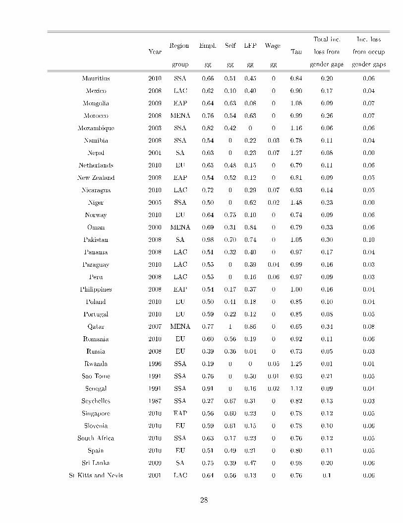
YearRegion Empl. Self LFP Wage

Tau

Total inc. Inc. loss

loss from from occup

group gg gg gg gg gender gaps gender gaps

Algeria 2004 MENA 0.78 0 0.79 0.06 0.94 0.31 0.05

Antigua 2001 LAC 0.49 0.45 0.01 0 0.76 0.05 0.04

Argentina 2010 LAC 0.48 0.33 0.29 0 0.89 0.13 0.04

Armenia 2008 CA 0.92 0.30 0.19 0 0.92 0.13 0.08

Australia 2008 EAP 0.37 0.48 0.17 0 0.79 0.09 0.03

Austria 2010 EU 0.60 0.46 0.14 0 0.74 0.10 0.05

Azerbaijan 2008 CA 0.81 0 0.02 0.07 1.10 0.04 0.04

Bahrain 2010 MENA 0.71 0.95 0.74 0 0.68 0.30 0.07

Bangladesh 2005 SA 0.64 0.65 0.69 0 1.33 0.28 0.08

28Variable 3: World Bank region (EAP: East Asia and Paci�c, EU: Europe, CA: Central Asia, LAC: LatinAmerica and the Caribbean, MENA: Middle East and North Africa, SA: South Africa, SSA: Sub-SaharanAfrica); variable 4: gender gap in employership (fraction of women excluded from employership relative tomen; source: own calculations from ILO data); variable 5: gender gap in self-employment (fraction of womenexcluded from self-employment relative to men; source: own results from ILO data); variable 6: gender gapin labor force participation (fraction of women excluded from the labor force relative to men; source: owncalculations from ILO data); variable 7: wage gender gap (female wage loss relative to males; source: ownresults); variable 8: Relative productivity self-employment (source: own results); variable 9: total income lossdue to gender gaps (source: own results); variable 10: income loss due to gender gaps in occupational choices(source: own results).

25

YearRegion Empl. Self LFP Wage

Tau

Total inc. Inc. loss

loss from from occup

group gg gg gg gg gender gaps gender gaps

Barbados 2004 LAC 0.75 0.57 0.07 0 0.84 0.09 0.07

Belgium 2010 EU 0.61 0.55 0.17 0 0.78 0.11 0.06

Belize 2005 LAC 0.47 0.25 0.48 0 0.90 0.19 0.04

Bhutan 2010 SA 0 0 0.07 0.02 0.98 0.02 0.00

Bolivia 2009 LAC 0.59 0.14 0.19 0 1.00 0.10 0.04

Bostwana 2006 SSA 0.48 0 0.09 0.02 0.98 0.05 0.03

Brazil 2009 LAC 0.52 0.38 0.26 0 0.91 0.13 0.04

Bulgaria 2010 EU 0.53 0.49 0.10 0 0.77 0.08 0.05

Burkina Faso 2006 SSA 0.68 0.61 0.16 0 1.15 0.12 0.07

Cambodia 2008 EAP 0.27 0.54 0 0 1.15 0.04 0.04

Cameroon 2001 SSA 0.47 0 0.03 0.03 1.20 0.03 0.01

Cape Verde 2000 SSA 0.50 0.07 0.15 0 0.97 0.08 0.03

Chad 1993 SSA 0.67 0.31 0.06 0 1.30 0.06 0.04

Chile 2008 LAC 0.47 0.17 0.41 0 0.92 0.17 0.03

Colombia 2010 LAC 0.57 0.08 0.32 0 1.09 0.13 0.03

Congo 2005 SSA 0.68 0 0 0.12 1.25 0.02 0.02

Costa Rica 2010 LAC 0.60 0.25 0.41 0 0.88 0.18 0.05

Cote d'Ivoire 2002 SSA 0.37 0.27 0.22 0 1.17 0.10 0.03

Cyprus 2010 EU 0.82 0.56 0.17 0 0.80 0.13 0.08

Czech Republic 2010 EU 0.64 0.54 0.25 0 0.84 0.14 0.06

Denmark 2010 EU 0.70 0.71 0.09 0 0.73 0.09 0.07

Djibouti 1996 MENA 0.32 0 0.45 0.23 0.99 0.18 0.03

Dominica 2001 LAC 0.47 0.38 0.35 0 0.96 0.15 0.04

Dominic Republic 2010 LAC 0.45 0.59 0.27 0 1.09 0.13 0.05

Ecuador 2010 LAC 0.55 0.02 0.36 0 0.98 0.15 0.03

Egypt 2007 MENA 0.80 0.13 0.73 0 0.82 0.29 0.07

El Salvador 2010 LAC 0.41 0 0.27 0.10 0.95 0.12 0.03

Estonia 2010 EU 0.76 0.68 0 0 0.72 0.08 0.08

Ethiopia 2005 SSA 0.75 0.57 0.14 0 1.11 0.11 0.07

Fiji 2005 EAP 0 0.27 0.56 0 0.97 0.21 0.01

Finland 2010 EU 0.65 0.58 0.06 0 0.78 0.08 0.06

France 2010 EU 0.68 0.65 0.10 0 0.75 0.09 0.07

Gabon 2005 SSA 0.45 0 0.28 0.08 1.11 0.11 0.02

26

YearRegion Empl. Self LFP Wage

Tau

Total inc. Inc. loss

loss from from occup

group gg gg gg gg gender gaps gender gaps

Georgia 2008 CA 0.49 0.39 0.13 0 1.06 0.08 0.04

Germany 2010 EU 0.62 0.57 0.15 0 0.74 0.10 0.06

Greece 2010 EU 0.61 0.35 0.33 0 0.92 0.15 0.05

Grenada 1998 LAC 0.38 0.09 0.32 0 0.86 0.13 0.03

Guatemala 2004 LAC 0.55 0 0.46 0.04 0.98 0.19 0.03

Honduras 2010 LAC 0.31 0 0.43 0.04 1.07 0.16 0.01

Hong Kong 2010 EAP 0.73 0.78 0.10 0 0.75 0.10 0.07

Hungary 2010 EU 0.52 0.56 0.13 0 0.75 0.09 0.05

India 2010 SA 0.67 0.26 0.65 0 1.30 0.26 0.04

Indonesia 2009 EAP 0.66 0.37 0.39 0 1.14 0.17 0.05

Iran 2008 MENA 0.85 0.40 0.80 0 1.03 0.32 0.07

Ireland 2010 EU 0.69 0.79 0.13 0 0.83 0.11 0.07

Israel 2008 MENA 0.75 0.66 0.13 0 0.75 0.11 0.07

Italy 2010 EU 0.58 0.44 0.32 0 0.87 0.15 0.05

Jamaica 2008 LAC 0.45 0.30 0.23 0 1.05 0.11 0.04

Japan 2008 EAP 0.72 0.67 0.29 0 0.75 0.15 0.07

Kazakhstan 2010 CA 0.35 0 0.05 0.02 0.97 0.04 0.02

Korea 2008 EAP 0.59 0.42 0.28 0 0.89 0.14 0.05

Kuwait 2005 MENA 0.76 0.97 0.66 0 0.69 0.27 0.08

Kyrgyzstan 2006 CA 0.56 0.31 0.27 0 1.03 0.13 0.04

Laos 2005 EAP 0.55 0.55 0 0 1.14 0.06 0.06

Latvia 2010 EU 0.49 0.49 0 0 0.74 0.04 0.04

Lebanon 2007 MENA 0.86 0.68 0.67 0 0.95 0.28 0.09

Lesotho 1999 SSA 0 0.13 0.22 0 1.38 0.09 0.01

Liberia 2010 SSA 0.23 0 0 0.06 1.25 0.01 0.01

Lithuania 2010 EU 0.67 0.54 0 0 0.75 0.06 0.06

Luxembourg 2010 EU 0.59 0.53 0.23 0 0.71 0.13 0.05

Madagascar 2003 SSA 0.30 0.32 0.04 0 1.13 0.04 0.03

Malawi 1987 SSA 0.92 0 0 0.10 1.38 0.02 0.02

Malaysia 2010 EAP 0.68 0.49 0.43 0 0.88 0.19 0.06

Maldives 2006 SA 0.76 0 0.42 0.10 0.79 0.19 0.06

Mali 2006 SSA 0.55 0.12 0.18 0 1.14 0.09 0.03

Malta 2010 EU 0.79 0.72 0.48 0 0.80 0.22 0.08

27

YearRegion Empl. Self LFP Wage

Tau

Total inc. Inc. loss

loss from from occup

group gg gg gg gg gender gaps gender gaps

Mauritius 2010 SSA 0.66 0.51 0.45 0 0.84 0.20 0.06

Mexico 2008 LAC 0.62 0.10 0.40 0 0.90 0.17 0.04

Mongolia 2009 EAP 0.64 0.63 0.08 0 1.08 0.09 0.07

Morocco 2008 MENA 0.76 0.54 0.63 0 0.99 0.26 0.07

Mozambique 2003 SSA 0.82 0.42 0 0 1.16 0.06 0.06

Namibia 2008 SSA 0.54 0 0.22 0.03 0.78 0.11 0.04

Nepal 2001 SA 0.03 0 0.23 0.07 1.27 0.08 0.00

Netherlands 2010 EU 0.65 0.48 0.15 0 0.79 0.11 0.06

New Zealand 2008 EAP 0.54 0.52 0.12 0 0.81 0.09 0.05

Nicaragua 2010 LAC 0.72 0 0.29 0.07 0.93 0.14 0.05

Niger 2005 SSA 0.50 0 0.62 0.02 1.48 0.23 0.00

Norway 2010 EU 0.64 0.75 0.10 0 0.74 0.09 0.06

Oman 2000 MENA 0.69 0.31 0.84 0 0.79 0.33 0.06

Pakistan 2008 SA 0.98 0.70 0.74 0 1.05 0.30 0.10

Panama 2008 LAC 0.51 0.32 0.40 0 0.97 0.17 0.04

Paraguay 2010 LAC 0.55 0 0.39 0.04 0.99 0.16 0.03

Peru 2008 LAC 0.55 0 0.16 0.06 0.97 0.09 0.03

Philippines 2008 EAP 0.54 0.17 0.37 0 1.00 0.16 0.04

Poland 2010 EU 0.50 0.41 0.18 0 0.85 0.10 0.04

Portugal 2010 EU 0.59 0.22 0.12 0 0.85 0.08 0.05

Qatar 2007 MENA 0.77 1 0.86 0 0.65 0.34 0.08

Romania 2010 EU 0.60 0.56 0.19 0 0.92 0.11 0.06

Russia 2008 EU 0.39 0.36 0.04 0 0.73 0.05 0.03

Rwanda 1996 SSA 0.19 0 0 0.05 1.25 0.01 0.01

Sao Tome 1991 SSA 0.76 0 0.50 0.01 0.93 0.21 0.05

Senegal 1991 SSA 0.91 0 0.16 0.02 1.12 0.09 0.04

Seychelles 1987 SSA 0.27 0.67 0.31 0 0.82 0.13 0.03

Singapore 2010 EAP 0.56 0.60 0.23 0 0.78 0.12 0.05

Slovenia 2010 EU 0.59 0.61 0.15 0 0.78 0.10 0.06

South Africa 2010 SSA 0.63 0.17 0.23 0 0.76 0.12 0.05

Spain 2010 EU 0.51 0.49 0.21 0 0.80 0.11 0.05

Sri Lanka 2009 SA 0.75 0.39 0.47 0 0.98 0.20 0.06

St Kitts and Nevis 2001 LAC 0.64 0.56 0.13 0 0.76 0.1 0.06

28

YearRegion Empl. Self LFP Wage

Tau

Total inc. Inc. loss

loss from from occup

group gg gg gg gg gender gaps gender gaps

St Vincent and the Grenadines 1991 LAC 0.52 0.34 0.47 0 0.88 0.19 0.04

Suriname 1998 LAC 0.75 0.59 0.52 0 0.86 0.23 0.07

Swaziland 1997 SSA 0.21 0 0.31 0.15 0.84 0.12 0.02

Sweden 2010 EU 0.70 0.68 0.11 0 0.75 0.1 0.07

Switzerland 2010 EU 0.60 0.38 0.16 0 0.74 0.10 0.05

Tanzania 2006 SSA 0.60 0 0 0.03 1.36 0.01 0.01

Thailand 2010 SA 0.60 0.32 0.16 0 1.01 0.1 0.05

Trinidad and Tobago 2005 LAC 0.49 0.42 0.33 0 0.85 0.15 0.04

Tunisia 1994 MENA 0.73 0.47 0.70 0 0.90 0.28 0.07

Turkey 2010 CA 0.81 0.52 0.60 0 0.90 0.25 0.08

Uganda 2003 SSA 0.51 0.24 0 0 1.18 0.03 0.03

United Arab Emirates 2008 MENA 0.80 0.96 0.77 0 0.67 0.31 0.08

United Kingdom 2010 EU 0.60 0.60 0.13 0 0.82 0.1 0.06

Uruguay 2010 LAC 0.53 0.21 0.14 0 0.90 0.09 0.04

Vietnam 2004 EAP 0.57 0.40 0.04 0 1.11 0.06 0.05

Yemen 1999 MENA 0.85 0.35 0.67 0 1.00 0.27 0.07

Zambia 2000 SSA 0.67 0.42 0 0 1.11 0.05 0.05

Zimbabwe 2002 SSA 0.44 0 0.08 0.14 1.08 0.05 0.02

29