uas pkdstl

8/11/2019 uas pkdstl

http://slidepdf.com/reader/full/uas-pkdstl 1/10

Nama : Dila Resti Wahyuni

No. Reg : 5115111691

M.K : Penggunaan Komputer Dalam Sistem Tenaga Listrik

Jawaban Bab 5

(5.1)

A 69-kV, three-phase short transmission line is 16 km long. The line has a per phase series

impedance of 0.125 + j0.4375 per km. Determine the sending end voltage, voltage

regulation, the sending end power, and the transmission efciency when the line delivers.

(a) 70 MVA, 0.8 lagging power factor at 64 kV.

(b) 120 MW, unity power factor at 64 kV.

Use lineperf program to verify your results.

The Line impedance is ( )( )

The receiving end voltage per phase is

√

a. The complex power at the receiving end is

( )

The current per phase is given by

( )

The Sending end voltage is

( )( )( )

The sending end line-to-line voltage magnitude is

( ) √ | | The Sending end power is

( ) ( )( )



Transmission line efficiency is

( )

( )

b. The complex power at the receiving end is

( )

The current per phase is given by

( )

The sending end voltage is( )( )( )

The sending end line to line voltage magnitude is

( ) √ | |

The sending end power is

( ) ( )( )

Transmission line efficiency is

( )

( )



(5.4)

Shunt capacitors are installed receiving end to improve the line performance of problem 5.3.

the line deivers 200MVA, 0,8 lagging power factor at 220 kV

a. determine the total Mvar and the capacitance per phase of the Y-connected capacitors

when the sending end votage is 220 kV. Hint: use (5.85) and (5.86) to compute the power

angel and the receiving end reactive power

b. use lineperf to obtain the compensated line performance

a. The complex load at the receiving end is

( )

For VR(LL) = 220 kV, from (5.85), we have

( )( ) ( ) ( )( )(

Therefore

( )

Or

now from (5.86), we have

( )( )( ) ( ) ( )( )

( )

therefore, the required capacitor Mvar is

| | ( ⁄ )

The required shunt capacitance per phase is

( )( )( )



SOAL 6.2

The values marked are impedances in per unit on a base of 100 MVA. The currents

entering buses 1 and 2 are

I1 = 1:38 - j2:72 pu

I2 = 0:69 - j1:36 pu

(a) Determine the bus admittance matrix by inspection.(b) Use the function Y = ybus(zdata) to obtain the bus admittance matrix. The



2

3

I

I2 j 0,5 j 1,0

0,0125 + j0,0250,01 + j0,03

0,4 + j0,2

1

function argument zdata is a matrix containing the line bus numbers, resistance and

reactance. (See Example 6.1.) Write the necessary MATLAB commands to obtain

the bus voltages.

Converting all impedances to admittances results in the admittance diagram shown in Figure

50

A. Determine the bus admittance matrix by insfection



2

3

I1 I2-j2 -j 1

16 - j3210 - j30

2 - j1

y12

y23 y13

10 – j20

KCL

I1 = y10V1 + y12(V1-V2) + y13 (V1-V3)

I2 = y20V2 + y21(V2-V1) + y23(V2-V3)

0 = y31(V3-V1) + y32(V3-V2)

Rearanging Equattion

I1 = (y10+ y12+ y13)V1- y12V2- y13V3

I2 = -y13V1+(y20+y21+y23)V2- y23V3

0 = -y31V1 – y32V2 + (y31+y32+y33)V3

Admittances

y11 = y10+ y12+ y13 = 20 - j52

y22 = y20+y21+y23 = 26 - j53

y33 = y31+y32+y33 = 28 - j63

y12 = y21 = - y12 = 10 - j20

y13 = y31 = - y13 = 16 - j32

y23 = y32 = - y23 = 10 - j30

1



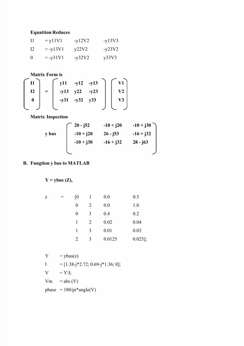
Equattion Reduces

I1 = y11V1 -y12V2 -y13V3

I2 = -y13V1 y22V2 -y23V2

0 = -y31V1 -y32V2 y33V3

Matrix Form is

I1 y11 -y12 -y13 V1

I2 = -y13 y22 -y23 V2

0 -y31 -y32 y33 V3

Matrix Inspection

20 - j52 -10 + j20 -10 + j30

y bus -10 + j20 26 - j53 -16 + j32

-10 + j30 -16 + j32 28 - j63

B. Fungtion y bus to MATLAB

Y = ybus (Z),

z = [0 1 0.0 0.5

0 2 0.0 1.0

0 3 0.4 0.2

1 2 0.02 0.04

1 3 0.01 0.03

2 3 0.0125 0.025];

Y = ybus(z)

I = [1.38-j*2.72; 0.69-j*1.36; 0];

V = Y\I;

Vm = abs (V)

phase = 180/pi*angle(V)



The result is

Y =

20.0000 -52.000i -10.0000 +20.000i -10.0000 +30.000i

-10.0000 +20.000i 26.0000 -53.000i -16.0000 +32.000i

-10.0000 +30.000i -16.0000 +32.000i 28.0000 -63.000i

Vm =

1.0293

1.0217

1.0001

phase =

1.4596

0.9905

-0.0150

uas pkdstl

Documents