u-N12 39 COMUTRTONAL FLUID DYNAMICS ON PRALLEL PROCESSORSCU) /IYALE UNIV NEUJ NAVEN CT DEPT OF CONFUTER SCIENCEWi D GROPP ET AL DEC 87 YALEU/DCS/RR-570 AFOSR-86-9898

UNLSSIFIED F,'G 28/4 M

mUNCLRsEEEEEomm iEE1~hhhEE

'AAK'

4.I

A-vA-

.2.V.-

'A'F.

A-

"A

'A,

"'p

'PA

N'.-A.

-P

A-N'-P

pA-.

VP.A-

n I~ ~HaaI El IIII~ _

- 3L DVI~ 11111 ~-A. Hi **~ ~ ___I - U.' IIIII~p LIP=! =

IL. r liii to~ I i '~

* III I. I AllisIIIIII liii 1.8

liii'A- l*a

II~

I~. - 11111=

-A

-p- 4..--"A-

-P-

-A4-A"

Np-WA..

V..'p

S

sicN

0.!r

'A-(N'A.-

A---A-Vp-

A--.-.

-1~

*hj~

4-.4-

Si ~AVAD ~,AA$-~ *~,.-.-V V V V V V V V V V V V..A- t

%4-% A%/At ~ ~ -A, ~ ;&$~z~~AA. -'<;K-. '.'- - ~ ~

A- . . N' %AV.-y%4 ~

A.. A~~V

'P ~

,_ r,, gl FILE p,

C3)

DTIC

ELECT5

4

. Ivy,-

*,..e €". flf' - w", rr] , . ,- ,.-e -wf.,"

.1 h - * 1 -'I " l -

TV

YALE UNIVERSITYDEPARTMENT OF COMPUTER SCIENCE

88 3 18 03I1~

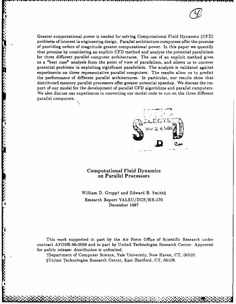
4Greater computational power is needed for solving Computational Fluid Dynamics (CFD)problems of interest in engineering design. Parallel architecture computers offer the promiseof providing orders of magnitude greater computational power. In this paper we quantifythat promise by considering an explicit CFD method and analyze the potential parallelismfor three different parallel computer architectures. The use of an explicit method givesus a "best case" analysis from the point of view of parallelism, and allows us to uncoverpotential problems in exploiting significant parallelism. The analysis is validated againstexperiments on three representative parallel computers. The results allow us to predictthe performance of different parallel architectures. In particular, our results show thatdistributed memory parallel processors offer greater potential speedup. We discuss the im-port of our model for the development of parallel CFD algorithms and parallel computers.We also discuss our experiences in converting our model code to run on the three differentparallel computers.

.-"r, -. rC "7 -

a.Z4 1988

Computational Fluid Dynamicson Parallel Processors

William D. Groppt and Edward B. Smitht

Research Report YALEU/DCS/RR-570December 1987

This work supported in part by the Air Force Office of Scientific Research undercontract AFOSR-86-0098 and in part by United Technologies Research Center. Approvedfor public release: distribution is unlimited.

tDepartment of Computer Science, Yale University, New Haven, CT, 06520.tUnited Technologies Research Center, East Hartford, CT, 06108.

%

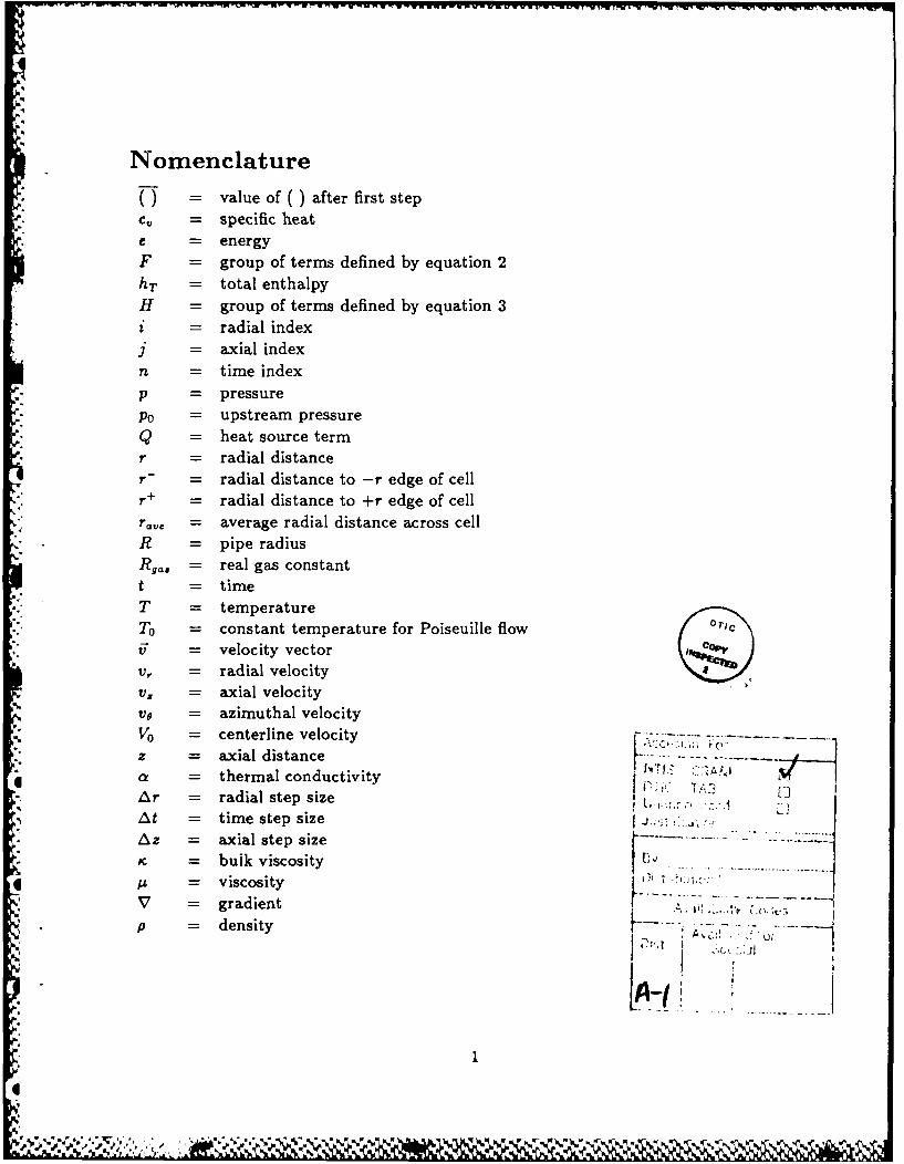
Nomenclature

() = value of ( ) after first step-" c = specific heate = energyF = group of terms defined by equation 2hT = total enthalpyH = group of terms defined by equation 3

= radial index= axial index

n = time indexp = pressure

PO = upstream pressureQ = heat source termr = radial distancer- = radial distance to -r edge of cellr + = radial distance to +r edge of cellrave = average radial distance across cellR = pipe radiusRga, = real gas constantt = time

T = temperatureTo = constant temperature for Poiseuille flowv = velocity vector

Vr = radial velocityv, = axial velocityv6 = azimuthal velocityV0 = centerline velocity . -

z = axial distancea = thermal conductivityAr = radial step size i I -3

At = time step sizeAz = axial step sizeK = bulk viscosity --.A = viscosityV = gradient .. ., .

p = d e n s it y 1.. . o i. ;

4

Introduction

Computational Fluid Dynamics (CFD) problems are among the most demanding scientificcomputing problems in terms of the computational resources they require. Currently,CFD problems are extensively solved on vector supercomputers, primarily Cray and Cyber.While current supercomputers have adequate computational power to solve CFD problemswhich are three dimensional or unsteady or viscous, extending CFD to problems which arethree dimensional and unsteady and viscous requires vastly more computational power.

One example of a computationally intensive CFD problem is modeling the air flow- through an airplane's gas turbine engine. The flow through a gas turbine engine is three

dimensional, unsteady and viscous. Further the geometry is extremely complex includingseveral turbine stages, several compressor stages and a combustor. Gas turbine engineersmust design the entire engine and would simulate the flow through the entire engine if thecapability were available. As an example of the computational intensity of CFD calcula-tions, Rai recently took over 100 hours on a Cray X-NiP to run a 3-dimensional viscous

* unsteady model for the air flow past two stator blades and a single rotor blade of an axialor flow gas turbine [Rai 87]. Although this run time is far too excessive for the use of such

a code in engin- ering design, only part of the gas turbine was modeled. As the Cray isA on of the fastest machines in the world and near the physical limits on the speed of aA uni-processor, no existing computer is fast enough for these calculations.

To speed needed calculations up several orders of magnitude faster supercomputers are% needed in gas turbine engine design. Computer processors, however, are reaching their

physical speed limits. Processor designs appear to be within a single order of magnitude oftheir speed limits due to physical limitations such as the speed of light and gate switchinglimits. Therefore needed throughput cannot be achieved with single processor computers.

inParallel processor computers offer the possibility of achieving the throughput neededfor CFD. Researchers are now investigating the effectiveness of using parallel computersthe the solution of CFD problems [Jame 87,John 87]. The need to understand and exploit

pth architecture of parallel computers, however, makes it unclear whether we can design* parallel algorithms which will achieve the needed throughput for CFD problems.

To test the promise of parallel computers, we consider a model CFD problem andapply it to representatives of several types of parallel computers. This model is based onan explicit difference technique and thus has the greatest opportunities for parallelism (as

Z compared to implicit difference techniques). For each class of parallel computer, we develop* a time complexity model and validate it against our model problem. These complexity

estimates are analytical estimates of the computer time needed to solve a CFD problem.The complexity estimates are expressed in terms of basic machine and problem parameters,such as floating point and communication speeds and number of grid points. From theseestimates, we can estimate the performance of CFD codes on supercomputers utilizingsignificant parallelism.

2

,,mr.- . . . r - u--u" :-, ", - ,T I~ an . .,: '' , - k ; - -. = - ,, a r

Finally, we discuss our experiences in using parallel computers for solving CFD prob-lems.

1 Architectures

A number of different types of parallel architecture computers are available today. Theserun from very fine grain machines such as vector processors and very long instructionword machines to large numbers of almost independent processors. In this paper, we

will consider three architectures which represent an important part of the spectrum ofpossible parallel computers. These are multiple vector processors, tightly coupled MIMDand loosely coupled MIMD.

Multiple vector processors consist of several vector computers operating in parallel.Exchanges of information and synchronization between the processors is facilitated by

special high-speed hardware. Examples are the Cray X-MP, Cray 2, ETA 10, and the* Alliant FX/8, that last of which was used in this study.

Tightly and loosely coupled MIMD computers work on essentially independent data inparallel, with differing kinds of access to each other's data.

Tightly coupled MIMD computers are collections of independent processors which areclosely connected, usually by shared memory. A parallel program running on this typeof machine consists of independent threads of control which may access each other's data

.. -, and can tightly control each other's operation by manipulating this shared data.The advantage of the tightly coupled MIMD approach is that there is no single thread

of control, and hence no a-priori serial execution. There have been a number of machinesof this type built by recent startup companies, such as the Encore Multimax 120, used inthis study and the Sequent Balance series.

Loosely coupled MIMD machines are collections of independent processors which com-municate through some reliable mechanism, but which don't directly share any data. In-stead, all interprocessor sharing of data is done by I/O operations, typically the sendingand receiving of message packets. This provides a measure of programming safety and re-producibility of results often absent in shared memory (tightly coupled MIMD) machines,since all modifications to "shared" data structures is handled explicitly by the programmer,rather than implicitly through a shared memory access. However, most systems currentlyon the market have a high overhead associated with interprocessor communication.

Example machines of this type include the various hypercubes from Intel, NCUBE, andothers, and some research machines, such as the LCAP system of IBM. The systems them-selves vary from a few, fast processors (LCAP) to many slow processors (Intel Hypercube).The Intel Hypercube was used in this study.

.i¢3

2 Finite Difference Algorithms

Finite difference algorithms used in Computational Fluid Dynamics for time accurate cal-culations can be divided into two major types: explicit and implicit.

With explicit finite difference algorithms the value of a variable at the new time isdetermined from the values of the variables at the old time directly (that is explicitly)without dependence on the values at the new time. Practically speaking this means thatthe values of the variables can be determined without solving a system of equations. Thetime step size that can be taken is limited by a time step on the order of the Courant-Freidrichs-Lewy (CFL) criterion (the smallest value of the time for a particle traveling atthe local fluid velocity to cross a finite difference grid interval). In many applications theGFL time step is much smaller (often orders of magnitude smaller) than the time steprequired for accurate calculation of the time variation of the variables.

The model problem studied here uses MacCormack's algorithm [MacC 69] which waschosen for its simplicity and wide familiarity to the CFD community. Major features ofMacCormack's algorithm are:

*An explicit difference scheme which is second order accurate in space and first orderaccurate in time.

a A two step scheme in which the present time values are used to calculate the inter-mediate values in the first step, and the present time and intermediate values areused to calculate the values at the new time.

Implicit finite difference algorithms differ from explicit finite difference algorithms inthat the determination of the values of the variables at the new time depends (implicitly)on the values of the variables at the new time. The advantage of a well-chosen implicitscheme is that numerical stability can be achieved with a time step size much greater thangiven by the explicit CFL limit [Jame 83].

The price to be paid by most implicit schemes is that the solution of a system ofequations is required at each step. Except for the solution of a tightly banded linear

0 system it is often faster to solve the linear system iteratively.We left implicit schemes for later study in order to address the basic question of whether

parallel architecture computers were applicable to solving CFD problems. We intend tostudy implicit schemes and linear solution techniques in future work. The use of sparse ma-trix methods in CFD problems is an area of current research on serial computers [Wigt 85]

as well as on parallel computers.

* 3 Model Problem

Descriptions of the physical model problem, its geometry, its mathematical formulation,and the numerical solution method follow.

4

5,.-.*

0:

The physical model problem we consider is unsteady compressible viscous flow throughan insulated duct. We further assume the flow to be axisymmetric with swirl. A timedependent model problem was chosen for this study since time marching schemes are

generally used in CFD for both steady and unsteady problems. A two dimensional problemwas chosen both to provide a start at physically reasonable models for combustor flow

and to introduce the complexities of multi-dimensional problems. For the model problemstudied here the fluid velocities and pressure are known so that the temperature can beobtained by integrating in time the energy equation which is linear in temperature. Thedensity was obtained from the perfect gas law.

The case studied was obtained from the model problem by assuming Poiseuille flow(parabolic velocity profile and linear pressure gradient) and treating the residual terms asa heat source. Poiseuille flow is an exact solution for steady, incompressible, isothermal,viscous pipe flow. We wished to retain the compressible effects in case they affected the

parallelization of the code. Poiseuille flow does not exactly satisfy the compressible flowequations. There are residual terms which are collectively treated as a heat source. Thusthe solution to the case studied was steady Poiseuille flow and, in particular, constanttemperature. This facilitated debugging.

The geometry of the model problem is a rectangular domain with a tensor productmesh. The left side is the inflow and the right side is the outflow. The top is the insulatedwall, and the bottom is the centerline of the cylinder.

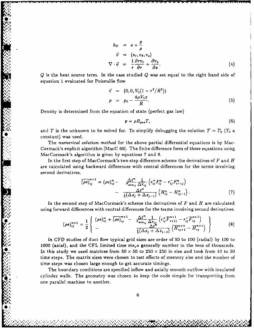
The mathematical formulation of the energy equation in cylindrical coordinates is givenby equations 1 through 6.

dpe 1arF aH-- + -- + - = Q (1)a ar r z

where

F = pvhT - + .) -c(V . Iv,

"a ra 3-A' (2vv.+ ve a v v' v (a v- + 8v 2 \(20- T ar r a) z (2)

and

,H pvhT- a-+ IC(V )v,

:2v-. + V, a~ + a + (3)aVz /z

where

e = p(v. 2 + cuT)

5Pt.

-p%

hT = ep

= (Vr,,vV.)1 arv, v,(

V -- r- ar dz (4)

Q is the heat source term. In the case studied Q was set equal to the right hand side of

equation 1 evaluated for Poiseuille flow

- (0, 0, Vo(1 - r2 /R 2 ))

P IN ~4ttV0z(5.." zV::P P0 R (5)

Density is determined from the equation of state (perfect gas law)

p = pR 9aST, (6)

and T is the unknown to be solved for. To simplify debugging the solution T = To (To a

constant) was used.The numerical solution method for the above partial differential equations is by Mac-

Cormack's explicit algorithm [MacC 691. The finite difference form of these equations usingMacCormack's algorithm is given by equations 7 and 8.

In the first step of MacCormack's two step difference scheme the derivatives of F and H

" are calculated using backward differences with central differences for the terms involvingsecond derivatives.

n"-- + I , _ A t" 1 (r+ F n -r ,..F j'.j_1(pe),, = (pe)7- t r.atj Arq -

Atn H, d.(Ca

j + AH n) - , _ ) . (7 )

In the second step of MacCormack's scheme the derivatives of F and H are calculated

using forward differences with central differences for the terms involving second derivatives.(pe)!' (Pe) n" I- At" 1 (+,",_+ - ,F , )

(pe) ' = At n+1 -+ 1) + (8)L(Azj + Az,_-1)

In CFD studies of duct flow typical grid sizes are order of 50 to 100 (radial) by 100 to1000 (axial), and the CFL limited time steps generally number in the tens of thousands.

In this study we used matrices from 50 x 50 to 250 x 250 in size and took from 10 to 50time steps. The matrix sizes were chosen to test effects of memory size and the number oftime steps was chosen large enough to get accurate timings.

The boundary conditions are specified inflow and axially smooth outflow with insulated

* cylinder walls. The geometry was chosen to keep the code simple for transporting fromone parallel machine to another.

6

0Py'l

4 Time Complexity Model

In order to understand the potential of parallel programming for CFD problems, we needto develop models which will allow us to predict the performance of a parallel computer.Time complexity models are constructed for each of the three classes of parallel computersused in this study. Since the time complexity model is an analytic expression for the

computer time needed to solve a problem, based on fundamental parameters of the modelproblem and the computer, we can use the complexity estimates to predict the performanceof new parallel computers and suggest which architectures offer the most potential for CFD

problems.In this section we will first give some basic definitions, then explain superlinear speedup.

Then we will give time complexity estimates for simple stencils and apply and extend theseestimates to our model problem.

We will denote the time complexity by T(p, n), where p is the number of processors

and the problem is on an n x n mesh. Another useful measure is the speedup, s, defined

by s(p,n) = T(1,n)/T(p,n). In a perfectly parallel algorithm with perfect hardware andsoftware, T(p,n) = T(1,n)/p. Algorithms, hardware, and software are not, however,

perfect and this section is concerned with modeling the "imperfections." We therefore

define the computational efficiency as T(1, n)/(pT(p, n)). A perfect parallel computer andalgorithm has a computational efficiency of 1.

The nature of these imperfections depends on the type of parallel computer. However,

they are related to the access to memory. In a loosely-coupled MIMD parallel processor,it is the interprocessor communication time, which can be thought of as access to remote

- memory, which is important. In a tightly-coupled MIMD parallel processor, it is the accessto shared memory, and the establishment of critical regions (access control to memory)which is important. In a multiple vector parallel processor, it is the access to shared

memory again and cache contention among the processors which is important. In addition,various "non-parallel" operations may reduce the possible speedup.

4.1 Superlinear speedup

As an example of how memory access can affect the time complexity on parallel computers,we discuss a commonly misunderstood phenomena called superlinear speedup. Superlin-

ear speedup is a speedup higher than the speedup of a "perfect" parallel computer andalgorithm-that is, a computational efficiency greater than 1. This effect is real, and it is

caused by "non-linear" features in the description of the parallel computer.In particular, it is evident if the process of breaking the program into a number of

parallel pieces produces smaller pieces which can use the hardware more effectively.An example is a machine where each processor has a memory cache of size C let the

7

I%

time to run a problem of size m on p processors be

T.,(p) = m + g(m,p)P

mpwhere - fm/p if m/p> Cp 0 otherwise.

-"The g represents the time to fill the cache from memory if the cache can not hold the entireS•"problem (i.e., T,(1) = 2m) then, as p -+ 00,

Tm (1) -_ 2,

*5,. (5,)

twice the "perfect" speedup.Now, if instead we insist that m be "large enough", ie., m > pC, then we leave the

regime where the problem fits in the cache, and the speed up is linear:

Tm (1)

pTm(p)

as both p and m go to infinity.This effect is important in modern parallel computers because the relevant "cache size"

has become very large. For example, in a tightly-coupled MIMD shared memory machinelike the BBN Butterfly, the cost for accessing non-local memory is roughly three times thatof local memory. Thus the entire local memory (several megabytes) can be considered the"cache" for the purposes of this argument. This effect can generate anomalous results forsmall problems.

4.2 Time complexity estimates for simple stencils

In order to motivate our choice of complexity model, we first develop a model for finitedifference schemes with 5 and 9 point stencils for the three parallel architectures used in thisstudy. Using these results, we can construct a model which predicts the time complexity

of our model problem. We also discuss some global operations which are present in ourmodel algorithm, and how they are handled on different computer architectures.

We first establish some basic ideas concerning two main classes of parallel programmingstyles: message passing and shared memory. We first describe these two approaches andthen discuss the similarities in terms of both expressiveness and of efficiency.

In a message passing computer, memory access for data on different processors is viainter-processor communication which is handled by explicitly sending a message from oneprocessor to another. There are two major parameters of interest. These are the message

startup time a, and the transfer rate r. To make a and r independent of particularhardware implementations, a and r have been nondimensionalized by dividing by the

8

floating point speed in flops/sec. Thus a is in ops/startup and r is in ops/word. We willdenote the floating point computation rate by f flops/sec.

For the tightly coupled computers, memory access is from shared memory to processorand the three parameters of interest are the memory access time, the speed of a floatingpoint operation and the number of simultaneous memory references. The programmingconstructs used with shared memory machines include barriers and critical regions. Abarrier is a synchronization point which all processors must reach before any of them canproceed. A critical region allows only one process to access and modify data at a time. Ina parallel program, barriers may be used, for example, to wait for all processors to reachthe end of a time step. A critical region may be used to provide a unique do-loop indexto each parallel processor. These are discussed in more detail in, e.g., [Andr 851.

Message passing computers such as the Intel Hypercube and shared memory machinessuch as the Encore Multimax are often considered two completely different types of parallel

. computer. In fact, when viewed in the right way, they are very similar. What distinguishesthem is the relative cost of referencing remote or shared information. The following table

*_ shows the correspondence between the costs of interprocessor communication for the twotypes of machines.

Message Passing Shared Memory

I/0 startup time Cache miss overhead and timeto establish critical regionsand barriers

Transfer rate Memory transfer rate

Each of these machines have different strengths. The shared memory machines have fasteraccess to shared information, but pay a . enalty in terms of higher overheads in the formsof barriers and critical regions. In general, these barriers and critical regions are intrinsicto the multiprocess computation and are therefore unavoidable. Message passing machineshave simpler access control but at a higher cost in sharing data. Barriers and critical regionsare sometimes used with message passing computers; however, the style of programmingnormally used with message passing makes them less important.

Consider the cost of computing a step of an explicit PDE on an n x n (in 2-d) and ann x n x n (in 3-d) grid. This step will usually consist of an estimate of the time step size touse, based on CFL estimates, followed by the application of a local stencil. The estimate ofthe time step requires global information (the solution everywhere); the application of thestencil just local or neighbor information. We describe first the local communication andthen the global communication. Since these effects are most noticable in the context ofmessage passing, we describe them in those terms. However, similar considerations applyto shared memory.

%. .0 ... 1 U lr = i- : : -

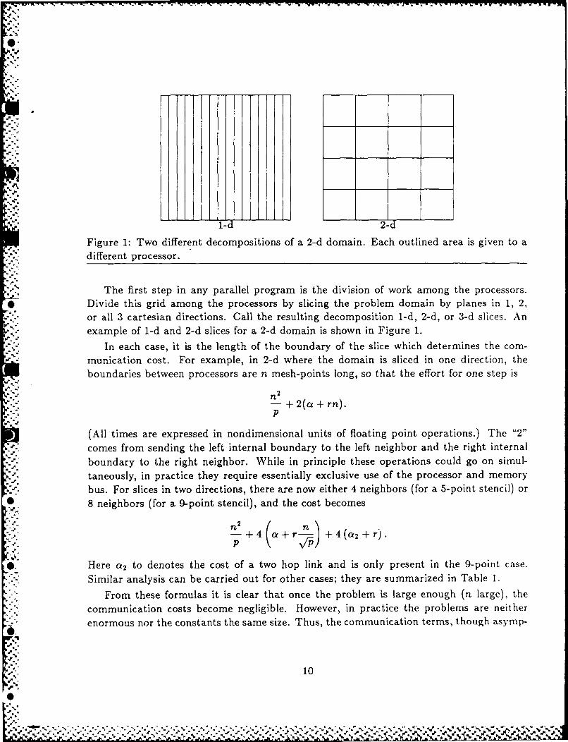
Figure 1: Two different decompositions of a 2-d domain. Each outlined area is given to adifferent processor.

The first step in any parallel program is the division of work among the processors.* Divide this grid among the processors by slicing the problem domain by planes in 1, 2,

or all 3 cartesian directions. Call the resulting decomposition 1-d, 2-d, or 3-d slices. Anexample of 1-d and 2-d slices for a 2-d domain is shown in Figure 1.

In each case, it is the length of the boundary of the slice which determines the com-4,. munication cost. For example, in 2-d where the domain is sliced in one direction, the

boundaries between processors are n mesh-points long, so that the effort for one step is

n + 2(a + rn).p

(All times are expressed in nondimensional units of floating point operations.) The "2"

comes from sending the left internal boundary to the left neighbor and the right internal

boundary to the right neighbor. While in principle these operations could go on simul-

taneously, in practice they require essentially exclusive use of the processor and memory

bus. For slices in two directions, there are now either 4 neighbors (for a 5-point stencil) or

* 8 neighbors (for a 9-point stencil), and the cost becomes

n n+4a+r- J +4(a 2 + r) .

P fP)

*Here a 2 to denotes the cost of a two hop link and is only present in the 9-point case.

Similar analysis can be carried out for other cases; they are summarized in Table 1.

From these formulas it is clear that once the problem is large enough (n large), the

communication costs become negligible. However, in practice the problems are neither

enormous nor the constants the same size. Thus, the communication terms, though asyrnp-

01

4,%

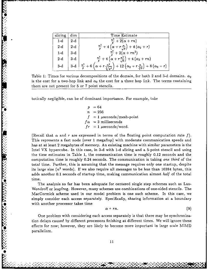
slicing dim Time Estimate

2-d 2-d "2+4(a+rS)+±4(a 2 ±r)1-d 3-d nl3 + 2(a + rn2)2-d 3-d +4 (a + +4 (a 2 + rn)

3-d 3-d !I--6ar +12(a + )+8(as-r

Table 1: Times for various decompositions of the domain, for both 2 and 3-d domains, a 2

is the cost for a two-hop link and a 3 the cost for a three hop link. The terms containingthem are not present for 5 or 7 point stencils.

totically negligible, can be of dominant importance. For example, take

p = 64n = 256f = 1 /iseconds/mesh-point

fa = 3 millisecondsfr = 1 useconds/word.

(Recall that a and r are expressed in terms of the floating point computation rate f).This represents a fast node (over 1 megaflop) with moderate communication speeds andhas at at least 2 megabytes of memory. An existing machine with similar parameters is theIntel VX hypercube. In this case, in 3-d with 1-d slicing and a 5-point stencil and usingthe time estimates in Table 1, the con-munication time is roughly 0.12 seconds and thecomputation time is roughly 0.24 seconds. The communication is taking one third of the

total time. Further, this is assuming that the message requires only one startup, despiteits large size (n 2 words). If we also require all messages to be less than 16384 bytes, thisadds another 0.1 seconds of startup time, making communication almost half of the totaltime.

The analysis so far has been adequate for centered single step schemes such as Lax-Wendroff or leapfrog. However, many schemes use combinations of one-sided stencils. The

MacCormick scheme used in our model problem is one such scheme. In this case, wesimply consider each access separately. Specifically, sharing information at a boundarywith another processor takes time

a + rn. (9)

One problem with considering each access separately is that there may be synchroniza-tion delays caused by different processors finishing at different times. We will ignore theseeffects for now; however, they are likely to become more important in large scale MIMD

parallelism.

-- 11

.

A certain amount of global communication is necessary in these algorithms as well. Forexample, the choice of time step size requires the global value of the maximum velocity. Inaddition, the values of interest in the computation include integrals along the boundary,which may need to be computed across processors. These operations fall into the generalcategory of reductions: taking data from many places and combining it to produce a singleresult.

Reductions are often done using a fast distribution algorithm such as those in [Saad 85],with the operation (maximum or sum) inserted into the distribution. For example, a tree-based distribution algorithm such as those described in [Saad 85] is fast on both sharedmemory and hypercube/message passing computers. In this case, the time to reduce pitems is

(a + r + f) logp

assuming simultaneous send/receives. One potential problem here is possible round-offerror; to avoid that, we reduce upward using the tree to a single node, then distribute that

single value downward to all nodes, again using the tree. The time is then

(2(a + r) + f) logp. (10)

When using a small number of processors and a shared-memory or complete intercon-

nect, it is often easier for a single processor to compute the reduction, then make thatvalue available to all processors. In this case, the time is pf plus the time to establish

two barriers, one before the reduction to insure that the data is ready, and one after it to- insure that the result is ready.

4.3 Time complexity estimates for the model problem

Our model problem is more complicated than a simple 5-point explicit scheme because itis multistep and each step is not centered. However, we can break it down into

o floating point work

- local data exchanges

* global data exchanges.

This form is suitable to a program where the parallelism is expressed explicitly. In our"'"" particular implementation, we can write the total computation time per step as

02T = F- + F2 - + 8"global reduce" + 6 ("send in y" + "send in x") (11)

P Py

where F1 is the floating point time per mesh point for operations on the whole grid, F'is the floating point time per mesh point for operations along one boundary, the grid isn x n, p is the number of processors, and p, is the number of processors in the y direction.

12

%

V.

Using equations 9 and 10 as the communication model, equation 11 becomesT= 2 FI + n n\ /

T - -+(a+r) logp+6 a+ +6 a+r-). (12)P Py P Py

The memory access terms Liii equation are the direct communication terms involving a

and r.

For this local communication model to be applicable, it must be possible to map a gridonto the parallel processor in such a way as to make adjacent slices adjacent in the parallel

processor. We will assume that any 2 or 3-d grid of interest can be efficiently embedded in

the parallel processor. Such embeddings are easy on hypercubes; alternatively, everything

we say here applies equally well to a mesh connected processor of the correct dimension.

For a shared memory machine with sufficient memory bandwidth, the figures are sim-ilar, except the global reduction is done differently, and the overhead of data sharing is

slightly different. In this case, the results aren 2 nT = F 1- + F2- + 16"barriers for reduce" + 6"barriers for data". (13)

P Py

Here, the "barriers" are synchronization points in the code. Depending on the implemen-

tation, these can be order p or log p. Further, it is possible to reduce the number of these

. by using barriers with values [Eise 87].

On a tightly coupled multiple vector processor such as the Alliant FX/8 the work es-

timates are slightly different. In these machines, "close coupling" of the processors allowsthe rapid transfer of information from one processor to another, and extremely fast syn-chronization. On the negative side, since there is no explicit parallelism, the programmer

may be dependent on the Fortran compiler to generate parallel code and it is possible forthere to be substantial amounts of non-parallel code generated. Further, any shared mem-

ory machine suffers from a potential bottleneck in memory access; depending on cache

or register utilization and the exact pattern of operations chosen by the compiler, the

performance may exhibit anything from superlinear speedup to a plateau in performance.

We can model this bottleneck in shared resources such as memory as follows. Let the

computation consist of two parts: one which is arbitrarily parallel, and one which uses the

shared resource. For example, consider a machine with p processors in which p floating

point operations may be done in parallel. However, only k processors may use the shared

memory at any time. Then the time to do a computation has the form

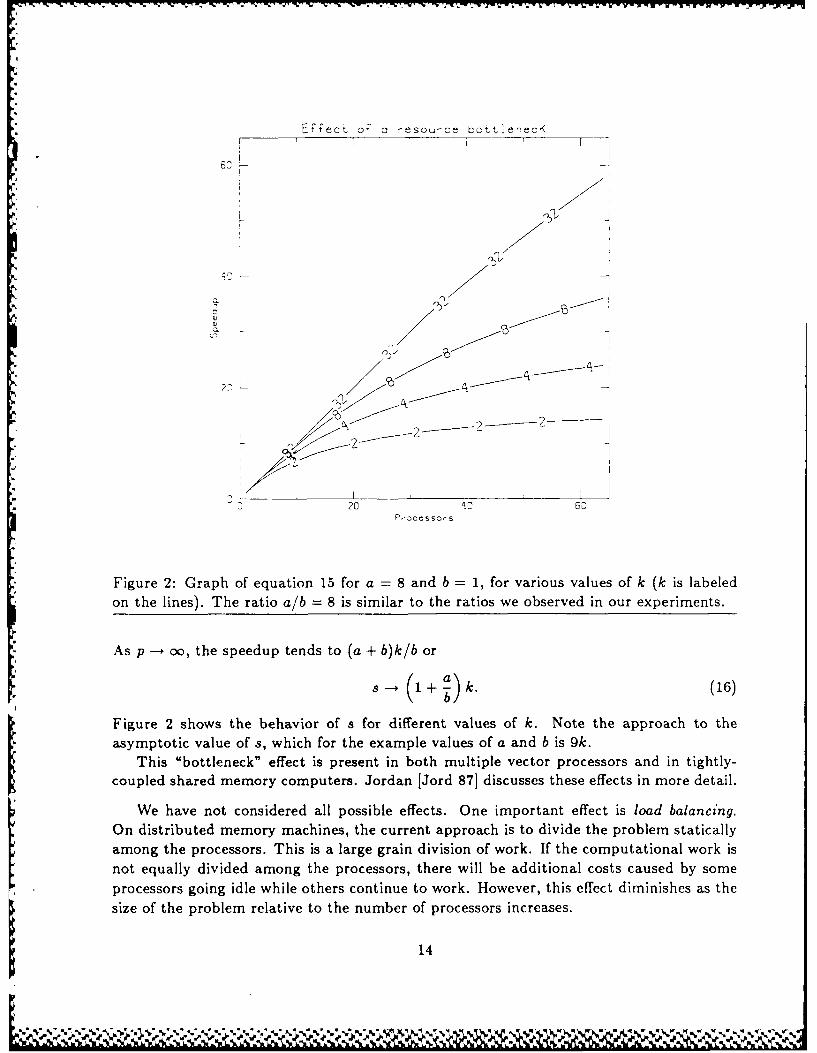
Sa bT p) + .(14)

p min(p,k)

For k = 1, this is the well-known Amdahl's law. The speedup predicted for such a machine

as p gets large (p > k) is

a+ b (a + b)kp (15)S P a+ b ak +bp

p min(pk)

13

A

EFect oT o resou-ct bottle-ecK

2-----

2 2

2 0

Pl-ocesso'-s

*Figure 2: Graph of equation 15 for a 8 and b 1, for various values of k (k is labeled* on the lines). The ratio a/b = 8 is similar to the ratios we observed in our experiments._

As p -- oo, the speedup tends to (a + b)k/b or

S 1~ + a)k. (16)

asymptotic value of s, which for the example values of a and b is 9k.This "bottleneck" effect is present in both multiple vector processors and in tightly-

coupled shared memory computers. Jordan [Jord 87] discusses these effects in more detail.

We have not considered all possible effects. One important effect is load balancing.

On distributed memory machines, the current approach is to divide the problem staticallyamong the processors. This is a large grain division of work. If the computational work isnot equally divided among the processors, there will be additional costs caused by someprocessors going idle while others continue to work. However, this effect diminishes as the

size of the problem relative to the number of processors increases.

14

5 Experimental Results

In this section we show the results of computing our model problem on several differenttypes of architectures.

We ran our model problem on three different parallel computers. An Intel iPSC Hy-percube, an Encore Multimax 120, and an Alliant FX/8. The Intel Hypercube is a looselycoupled MIMD, the Encore is a tightly coupled MIMD, and the Alliant is a multiple vectorprocessor. Each of these represents a different class of parallel computer.

Figures 3, 4, and 5 show the results of our experiments. We have computed fits tothese experiments using the models developed in Section 4. These fits were obtained by anon-linear least-squares fit to the timing data, after scaling the timing data by n 2/p.

5.1 Intel iPSC Hypercube

The Intel iPSC Hypercube is an example of a loosely coupled MIMD computer. The pro-i •cessors are connected in a hypercube architecture, and communicate by sending messages

over a dedicated ethernet link (one per processor-pair). Each processor has 0.5 megabytes

of memory, and on our machine, there is an additional 4.0 megabytes of memory on anattached board.

Figure 3 presents the results of these experiments. Each computation represents 10

time steps over the grid. A fit to the data using equation 12 gives"n "' t2 nT = 0.066- + 0.014- + 0.861 logp + 0.0302(n, + nu) + 0.868, (17)

P P

where nr = n/pz and n. = n/Pu.In Figure 3, we see the effects of the uneven distribution of work among the processors

in the stepped increase in the speedup figures. Each processor has some fixed number of"slices", each of which has roughly n/p: x n/p. mesh points. If p. or py do not divide n,

then some processors have [n/p,] x [n/pJ and some have [n/p,.J x [n/pyJ. The relativedifference is approximately (assuming both p, and Pu don't divide n)

SPu

As the number of processors approaches n, the difference can be very large. The points in

p where there are jumps in the speedup for the 1-d decomposition are just those values of

* p which divide n, as can be seen in Figure 3. Note that the hypercube interconnections arenot of major importance; a 2-d mesh interconnection would give almost the same results.

5.2 Encore Multimax

The Encore Multimax is an example of a shared memory MIMD computer. There aretwo processors per board, along with a cache memory. These boards are connected to

15

Iz

%~ .. %p-~

,. -"N

2eC-pos:t:Cn 0t do-a , f'or n=75 Fit for 1-d decompost:on :i Y

3 - Fit for ',-d s'ioes i L Fit for n = IGO

It for - sices I. -f ,

F7". t ;- 2 - 3. ....

-- .___--___ ___ ____ ____ ___

t0

!30 10

'~-ocss~rsP ocessors0- i sLicos in x + n 50

0 - -d sh:oes In 75- 2-d sLccs o

ot o- :-a dcooposltion (In ,) Fit fo 2-d decomoos:tho, (soco-es;

3C Ft 1 100 Fi t fo T 1I

- - -- Fit -o, n 7 5 ------ Fi for 75

t. . Fit for n 0

,,

fo n 13

200

a ++ ++

,, -. z 30 6 ' :o ' Zlo ' 0P oo ol.~r Pro oe$$o'

I - , = 50 + - n 5o 75

+, _o- : 75 o n :170

. . o - 100

Figure 3: Speed up figures for the Intel iPSC hypercube. The graphs show fits as afunction of decomposition at a fixed problem size, and as a function of problem size forfixed decomposition. The same fit parameters were used in all graphs, and are drawn ascurves.

4.1

*0

.-*-;

-',."16

0'

a very fast bus, on which the shared memory resides. The computer runs UnixTM and

provides a time-sharing environment. One problem when doing timing measurements ina multi-user environment is that any parallel job is competing for processors with otherusers, mailer daemons, etc. Timings are thus somewhat erratic. Further, they don't reflectsynchronization problems well, since idle processes won't use CPU time, and "real time"

measurements are even more inaccurate on a time-sharing system. Thus, our results shownin Figure 4 are at best approximate. However, they do match our speedup estimate very

well with parameters in equation 18, which is a combination of equation 13 and equation 14.

n 2 n 2 n/

T = 0.059- + 0.0080 + 0.08- + 0.29p. (18)p in (p, 0) P.

These parameters give a very good fit to our experimental data as shown in Figure 4.Note that since the onset of the "bottleneck" term is so high, this may be due more to

the availability of processors than to limitations in the hardware. In fact, the Encore bus

is very fast relative to the speed of the processors, and we do not expect to see a significantdegradation for the number of processors available.

5.3 Alliant FX/8

The Alliant FX/8 is an example of a multiple vector processor computer. It has up to eight"computational elements", each of which is a vector processor. These processors share twohigh-speed caches, which in turn have a high speed channel to memory. It is possible forthe processors to exceed speed of the cache.

Computations were done for 51 time steps and mesh sizes of n = 50, 100, 150, 200, and250 on an eight processor Alliant FX/8. Figure 5 shows the speedups observed for variousproblem sizes compared to a fit against Equation 14. The fit used is

T = 0.00645 n 2 + 0.00085 n 2

p min(p, k)'

where k = 2.45. The fit is insensitive to k in the range 2 < k < 3.

The apparent super-linear speedup for two processors shown by the curves in Figure 5

is an artifact of the curve fit, causd by the rapid turn-down in speedup at three processors.

The data in Figure 5 show a dropoff below linear speedup as the number of processorsincreases. This dropoff is due in part to a memory bottleneck. The memory bottleneck

occurs when many processors require the same data from memory. In the Alliant FX/8 each

of the four quadrants of the fast cache memory can be accessed by any two computational

elements (processors) via a crossbar interconnect. When more than two computational

elements try to access the same data there is "cache contention" which is a form of memory

bottleneck. In addition cache and main memory are updated via hardware to maintain

memory system consistency. Thus if more cache memories were added there would be

!17

- I- Fitt -'o P ::: /

Y/

1- Fit 'or py. C "

- Fit o o-:

. Figure 4:SedpfgrsfrteEc e

siz isn = Thi ne laesae h aus fpuedfrta cre h sldln

repireet 4: pefcSpeedup firefo the shreEeitinfonefctsedpa ohl

S10 processors.

~18

O

-V.

-to.

Speedup orn AlIaont FX/Br., .' I I I

at Ln = 50 0n 100 X

" n = 150 -H

I 1

, z 2CO0

S a -250*

q L

".-.

2 49

-.

W Figure 5: Results for the Alliant FX/8. The fit usesT = 0.00645n 2/p + 0.00085n'/min(p, 2.45). The speedup is almost independent of theproblem size. The solid line represents a perfect speedup; note the deviation from this lineby both the experimental results and the theory at around three processors.

19

%0

a memory bottleneck as cache and main memories are updated to maintain consistency.Another part is due to some of the program running in serial (using only a single processor);this is due in part to the Fortran compiler on the Alliant, in a deliberate trade-off betweenease of use and maximum parallelism.

Memory bottleneck will occur in any shared memory parallel computer. Since memorybottleneck will cause a falloff in the speedup curve below linear speedup, it is a verysignificant limitation on shared memory parallel computers for massive parallelism.

5.4 Summary of experimental results

The agreement between the experiments and the complexity estimates is very good. Thecomplexity estimates capture the important contributions to the computation time. Thuswe can use the complexity results to predict performance for differing values of the param-eters, including the number of processors.

In the case of a distributed memory parallel computer, such as the Intel Hypercube,* -the time estimate for the computation has the form shown in equation 12. For simplicity,

we will consider the case p. = ut . Then the estimate can be simplified to

" 2 n nT = F 1 - + F 2 - +8(a+r) logp+12 a+ 1P)

Because of the log p term there is a value of p beyond which adding additional processorsactually slows the computation down. The maximum speed up is achieved when dT/dp

0, and is at

'F2 + 6r + V( F2 + 6r)2 + 32F 1 (a + r)

X/. = n16(a+r)

From this we can see that the the optimal number of processors depends on n. It can beshown that, as n ---- co and with this optimal p, the speedup tends to

An2

* logn"

Thus, the speedup for the distributed memory parallel computer (e.g., Intel Hypercube)increases without bound as the problem size and number of processors grow.

For a shared memory parallel computer, such as the Alliant FX/8 or Encore Multimax,0.. the time estimate for the computation has the form shown in equation 14. (Note that%4" the shape of the Encore and Alliant results are very similar; the terms corresponding to

equation 14 in both cases are the dominant terms.) The predicted speedup is independentof the problem size, as we observed experimentally. The parameters determined by ourexperiments give a maximum possible speedup of roughly 20 for the Alliant and roughly80 for the Encore. Of course, the number of processors available on both the Alliant andthe Encore were picked to match the available memory bandwidths. Other technologies

20

PA A ,P e LWNW

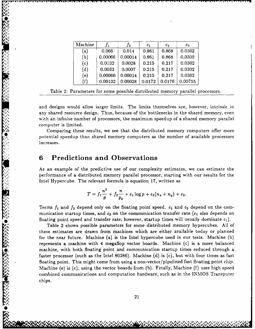
Machine h f2 cl C2 C3

(a) 0.066 0.014 0.861 0.868 0.0302(b) 0.00066 0.00014 0.861 0.868 0.0302(c) 0.0132 0.0028 0.215 0.217 0.0302

(d) 0.0033 0.0007 0.215 0.217 0.0302(e) 0.00066 0.00014 0.215 0.217 0.0302

(f) 0.00132 0.00028 0.0172 0.0176 0.00755

Table 2: Parameters for some possible distributed memory parallel processors.

and designs would allow larger limits. The limits themselves are, however, intrinsic inany shared resource design. Thus, because of the bottlenecks in the shared memory, evenwith an infinite number of processors, the maximum speedup of a shared memory parallelcomputer is limited.

Comparing these results, we see that the distributed memory computers offer more0. potential speedup than shared memory computers as the number of available processors

increases.

6 Predictions and Observations

As an example of the predictive use of our complexity estimates, we can estimate theperformance of a distributed memory parallel processor, starting with our results for theIntel Hypercube. The relevant formula is equation 17, written as

T fl- + f2- + cl logp+ c3(n, + n.) + C2 .P py

Terms f, and f2 depend only on the floating point speed. cl and c2 depend on the com-munication startup times, and c3 on the communication transfer rate (c , also depends onfloating point speed and transfer rate; however, startup times will usually dominate cl).

Table 2 shows possible parameters for some distributed memory hypercubes. All ofthese estimates are drawn from machines which are either available today or plannedfor the near future. Machine (a) is the Intel hypercube used in our tests. Machine (b)represents a machine with 4 megaflop vector boards. Machine (c) is a more balancedmachine, with both floating point and communication startup times reduced through afaster processor (such as the Intel 80386). Machine (d) is (c), but with four times as fastfloating point. This might come from using a non-vector/pipelined fast floating point chip.

Machine (e) is (c), using the vector boards from (b). Finally, Machine (f) uses high speedcombined communications and computation hardware, such as in the INMOS Transputerchips.

21

0

T 7 K T -- 7K; - K 'L- V-.' V- 1 '-V-I

ab c d e fp n T S T S T S T S T S T S

32 250 137 30 9.1 4.5 30 28 10 20 5.3 7.8 3.'4 2564 250 73 57 8.6 4.8 16 50 6.6 31 4 10 1.9 44128 250 41 101 8.6 4.8 9.6 86 4.7 44 3.4 12 1.1 7432 500 527 31 16 11 110 30 32 25 12 14 12 2864 500 268 61 12 13 57 58 18 45 7.9 21 6.2 53128 500 139 119 11 15 30 109 11 76 5.7 30 3.4 97256 500 1175 221 10 16 17 196 7 117 4.5 37 1.9 171

Table 3: Predicted times and speedups for various distributed memory parallel processors.Times are in the column T and speedups are in the column S.

In Table 3 we show the predicted performance of a number of possible distributedmemory parallel computers described in Table 2.

* The relatively poor showing of machines (b) and (e) is due to the large communicationterms, and suggests changes to both the algorithm (to reduce data exchanges) and thehardware (to make communication speeds comparable to floating point speeds). Thefigures for Machine (f) show that if comnmunication speeds (particularly startups, the "a"term) are increased, very respectable speedups can be obtained, even for large number ofprocessors. Similar calculations can be performed for proposed shared memory machines.

It is also interesting to compare the amount of programming work needed to run ourexperiments. In no case was much effort required to modify the original serial code to runon any of the parallel machines. The easiest to run was the Alliant, since the Fortran com-piler on the Alliant automatically makes reasonably good use of the parallelism. Neitherthe Encore nor the Intel machines have such compilers, and each required a small amountof special coding. In addition, the Alliant required some special coding to improve theperformance. The overall efforts were similar.

7 Conclusions

We have shown that significant parallelism is available at least for explicit methods forCFD. Our complexity estimates, validated by our experiments, show speedups limited

V only by the problem size for distributed memory architectures. For shared memory archi-

tectures, bottlenecks at the shared resource constrain the available speedups.In actual practice, our results show that the communications costs associated with

distributed memory parallel computers can seriously degrade the performance of thesesystems. Commercial shared memory computers such as the Alliant FX/8 have achieved

- a better balance of system components, at the (recognized) cost of limited parallelism.Since only massive parallelism has the promise of orders of magnitude increases in speed,

22

we hope that our results and ones like them will stimulate both algorithm and hardwaredesigners to overcome these practical problems.

In this paper we have considered shared memory and distributed memory parallelcomputers. In reality, actual computers are rarely so easily categorized. For example,a computer presenting the programmer with a shared memory model but implementedin hardware with several levels of distributed memory (a hierarchical memory) offers anintermediate form of parallel computer. The significance of our results is that, for signifi-cant parallelism, use of any shared resource that presents a bottleneck must be extremelylimited. The success of the distributed memory code shows that explicit CFD codes canbe easily written in such a form which avoids these bottlenecks.

Acknowledgements

The authors wish to thank James D. Wilson of AFOSR, Michael J. Werle and JosephR. Caspar of UTRC, and Martin H. Schultz of Yale University, for their comments andsuggestions.

References

[Andr 851 Andr6, F., D. Herman, and J.-P. Verjus, Synchronization of Parallel Programs,The MIT Press, Cambridge, 1985.

[Eise 87] Eisenstat, S., private communication, 1987.

[Jame 83] Jameson, A.: Transonic Flow Calculations. Department of Mechanical andAerospace Engineering, MAE Report 1651, Princeton University, July 1983.

[Jame 87] Jameson, A.: Successes and Challenges in Computational Aerodynamics. AIAApaper 87-1184, presented at AIAA 8th Computational Fluid Dynamics Conference,Honolulu, Hawaii, June 9-11, 1987.

[John 87] Johnson, G. M.: Parallel Processing in Fluid Dynamics. ISC Technical Report87003, Institute for Scientific Computing, Fort Collins, Colorado, paper presented atASME Fluids Engineering Conference, Cincinnati, Ohio, June 14-18, 1987.

[Jord 87] Jordan, H. F.: Interpreting Parallel Processor Performance Measurements. SiamJournal on Scientific and Statistical Computing, Volume 8, No. 2, pages s220-s226.

[MacC 69] MacCormack, R. W.: The Effect of Viscosity in Hypervelocity Impact Crater-ing. AIAA Paper No. 69-354, presented at AIAA Hypervelocity Impact Conference,Cincinnati, Ohio, April 30-May 2, 1969.

23

3Rai 87 Rai, M. M.: Unsteady Three-Dirnensional Navier-Stokes Simulations of Tu'lrbineRotor-Stator Interaction. AIAA paper 87-2058, presented at 23rd. Joint AIAA,'ASMEPropulsion Conference, San Diego, California, June 29-July 2, 1987.

[Saad 85] Saad, Y. and M. H. Schultz: Topological Properties of Hypercubes. Yale 'ni-versity Department of Computer Science Research Report Yale/DCS/RR-389, June,1985.

_Wigt 85 Wigton, L. B., N. J. Yu and D. P. Young: GMRES Acceleration of Computa-tional Fluid Dynamics Codes: AIAA paper 85-1494, presented at AIAA 7th Comnpu-

tational Fluid Dynamics Conference, Cincinnati, Ohio, July 15-17, 1985.

24

% .%N

* ~ .. ,~-.-.- - - = - 4-.-- - - - - J -w -. ~ - -. - - - S Sr.q

I

at

I,

I Lvi IF

I

4

.1a, 68Ja.,

'a,

S 0 S 0 0 0 S S S

.%%~~atI~a .~'- V