tyre shear force and moment descriptions and the ‘‘magic

Vehicle System Dynamics 0042-3114/03/3901-027$16.002003, Vol. 39, No. 1, pp. 27–56 # Swets & Zeitlinger

Tyre Shear Force and Moment Descriptions

by Normalisation of Parameters

and the ‘‘Magic Formula’’

R.S. SHARPy,* AND M. BETTELLAy

SUMMARY

Previous work by Radt on the use of normalised parameters to bring economy to the task of measuring,

describing and computing tyre shear forces and parallel works of Pacejka on the ‘similarity method’ are

reviewed, extended and applied. Similarity ideas are used in association with the ‘Magic Formula’. Some

published tyre force and moment results are divided into basic and nonbasic sets. The basic set contains a

notional minimum amount of information from which the full spectrum of results can be obtained by

applying similarity ideas. Calculations are carried out to show how the nonbasic results can be reconstructed

from the basic set. Advantages are obtained by using a novel nonlinear transformation of the longitudinal

and sideslip variables. The results are shown to be qualitatively excellent and quantitatively quite good. Of

course, the accuracy is not as high as with a full Magic Formula treatment but the economy is remarkable.

The process is captured in a MATLAB algorithm, included as an appendix. It is thought that this provides a

useful facility for enabling vehicle dynamics studies of a more generic flavour, in which circumstances

conspire to make high precision of tyre force descriptions inappropriate or impossible.

NOMENCLATURE

a1. . .a7 secondary Magic Formula coefficients

B, C, D, E primary Magic Formula parameters�BB, �CC, �DD, �EE normalised Magic Formula parameters

c�, c� variables in the slip transformations

Ccx tyre longitudinal carcass stiffness

Ccy tyre lateral carcass stiffness

CF� tyre cornering stiffness; function of load

CF� tyre camber stiffness; function of load

CF� tyre longitudinal slip stiffness; function of load

CM� tyre aligning moment stiffness; function of load

* Address correspondence to: R.S. Sharp, Electrical and Electronic Engineering, Imperial College of Science,

Engineering and Medicine, Exhibition Road, London SW7 2BT, U.K. E-mail: [email protected] School of Engineering, Cranfield University, U.K.

f�, f� functions used in slip transformations

Fx tyre longitudinal force

Fy tyre lateral force

Fy0 tyre lateral force for no longitudinal slip, used in

aligning moment calculations

Fz tyre load

Fx max maximum longitudinal force for no sideslip or camber;

function of load

Fy max maximum lateral force for free rolling and no camber;

function of load�FFx ¼ Fx=Fx max normalised longitudinal force�FFy ¼ Fy=Fy max normalised lateral force

�FFs ¼ffiffiffiffiffiffiffiffiffiffiffiffiffiffiffiffi�FF2

x þ �FF2y

qnormalised tyre shear force magnitude for combined slip

g1 constant relating to the influence of camber on peak

sideforce

int�, int� intercept variables in the slip transformations

m�, m� slope variables in the slip transformations

Mz tyre aligning moment

Mz max maximum aligning moment for free rolling and no

camber; function of load�MMz ¼ Mz=Mz max normalised aligning moment

Re tyre rolling radius

Sv vertical shift in Magic Formula

X, x, Y, y slip and force parameters in the Magic Formula

xp slip value for peak force

u forward velocity of tyre centre

� sideslip angle, slip angle

�p sideslip angle for peak sideforce

�Feq equivalent sideslip parameter, accounting for wheel

camber

� camber angle

� longitudinal slip, long slip, slip ratio

�p longitudinal slip for peak braking force

�� ¼ CF� � tan�=Fy max normalised sideslip parameter

��Feq normalised equivalent sideslip parameter for lateral

force, accounting for wheel camber

�� ¼ CF� � �=Fx max normalised longitudinal slip�� ¼

ffiffiffiffiffiffiffiffiffiffiffiffiffiffiffiffiffiffiffiffiffiffiffið��Feq

2 þ ��2p

Þ normalised combined slip��p normalised combined slip for which the force is a

maximum

� function of ��, defining Fx=Fy ratio in combined slip

28 R.S. SHARP AND M. BETTELLA

�0 ¼ �j �� ¼ CF� � Fxmax

CF� � Fymax

function of load;

� tyre spin velocity

1. INTRODUCTION

In respect to the longitudinal and lateral motions of road vehicles, the dominant

component of the external force system is from tyre=road frictional interactions. In

simulating such motions, it is crucial to represent the tyre shear forces with an

accuracy commensurate with the objectives of the simulation and in keeping with the

degree of detail in the treatment of the mass and the mass distribution of the vehicle.

Potentially, tyre force and moment computations are substantial consumers of

simulation time, such that they are virtually never calculated from a fundamental

physical tyre model, within a vehicle simulation, but rather via some empirical

method. The tyre shear force determination and the vehicle simulation are decoupled

in the interests of efficiency. Steady-state tyre forces and moments are regarded as

known functions of longitudinal slip, lateral slip, load, camber angle and possibly

inflation pressure and=or friction coefficient [1–5]. Additional relations may or may

not be included to accommodate tyre transient behaviour.

Contemporary alternative means for describing steady-state properties embrace

Magic Formula methods [6–13], the ‘‘HSRI’’ method [14], the ‘‘STI’’ method [15],

Radt’s methods [4, 16, 17] and Lugner’s method [18] among others. As can be judged

from the number of recent publications on the subject, the Magic Formula methods

are dominant, especially in Europe, and they are systematically gaining ground. They

can be characterised as powerful in terms of capacity for accuracy, time consuming in

terms of computation and very demanding in terms of parameters. The number of

parameters involved and their nature make the tyre testing necessary to derive their

values, lengthy, destructive of tyres themselves, expensive and very specialised.

Optimisation routines may well be needed to identify the parameters.1

In view of the robustness requirements of a vehicle=tyre combination in practice,

many studies in vehicle dynamics need a generically good representation of tyre shear

forces but they are not allied to a particular combination of vehicle, road surface, tyre

make, tyre pressure, tyre=surface temperature and state of wear. The capability of the

full Magic Formula method to rather precisely replicate extensive measurement

results is of little value in such circumstances. Advantages would come from having a

model with many fewer parameters, that are much more easily identified, and that

computes faster.

1 See http://www.automotive.tno.nl/vehicle dynamics; http://www.smithers-scientific.com/vehicle4

TYRE SHEAR FORCE 29

Radt’s ‘nondimensionalisation’ offers such possibilities [4, 16, 17]. Pacejka’s

‘similarity method’ [1, 10] provides an alternative. Normalisation of load and slip

variables is at the core of each scheme. The contention is that many relationships

become one and the same when expressed in normalised form and that the parameters

of the relationships can be determined from comparatively little test data. This paper

is an account of a test of normalisation, allied to the use of the Magic Formula, using

tyre test data from [6]. A portion of the test results included in [6] is used to construct

a full range of forces and moments. These forces and moments can be compared with

those measured ones not used in their prediction. The normalisation process is

necessarily developed, so that a full spectrum of results can be obtained, and useful

information is generated on the trading off of tyre test complexity and cost, parameter

evaluation complexity and accuracy of description of the forces and moments.

2. THE MAGIC FORMULA AND NORMALISATION OF PARAMETERS

The independent variables to be considered are longitudinal slip, �, lateral slip, tan�,

wheel load, Fz, and camber angle, �. Steady-state operation at constant tyre pressure

on a surface of constant friction properties will be presumed. The dependent variables

are longitudinal force, Fx, lateral force, Fy, and aligning moment, Mz. The Magic

Formula originates from [6] and the whole method based on it has moved through

several evolutions subsequently [7–13]. The formula itself is:

yðxÞ ¼ D sin½C arctanfBx EðBx arctanðBxÞÞg� with YðXÞ ¼ yðxÞþþ Sv and x ¼ X þ Sh ð1Þ

In the formula, Y(X) can be sideforce, longitudinal force or aligning moment while

(X) is the longitudinal slip or the sideslip. The longitudinal slip is a measure of the

tyre’s departure from free rolling. It is the ratio of the tread base material’s rearward

velocity and the modulus of the wheel centre forward velocity, given by:

� ¼ ðu þ Re � �Þ=juj ð2Þ

where Re is the tyre’s rolling radius, � is its spin velocity and u is the forward velocity

of its centre. At free rolling, �¼ 0, while for the locked wheel, �¼1. For a spinning

wheel, � will be positive and may rise without limit. The sideslip is the tangent of the

ratio of the negative of the lateral velocity of the notional centre of the contact patch to

the modulus of the forward velocity of the wheel centre. These definitions align with

SAE standards [19].

The basis of the formula is the idea that tyre force and moment curves under pure

slip conditions look like sine curves modified by stretching out the slip values using an

arctangent function. Figure 1 illustrates the relationship between the coefficients in


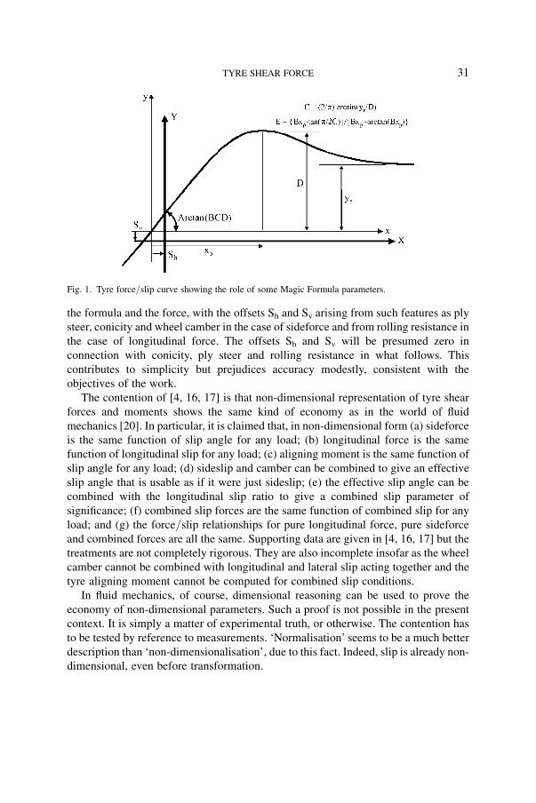
the formula and the force, with the offsets Sh and Sv arising from such features as ply

steer, conicity and wheel camber in the case of sideforce and from rolling resistance in

the case of longitudinal force. The offsets Sh and Sv will be presumed zero in

connection with conicity, ply steer and rolling resistance in what follows. This

contributes to simplicity but prejudices accuracy modestly, consistent with the

objectives of the work.

The contention of [4, 16, 17] is that non-dimensional representation of tyre shear

forces and moments shows the same kind of economy as in the world of fluid

mechanics [20]. In particular, it is claimed that, in non-dimensional form (a) sideforce

is the same function of slip angle for any load; (b) longitudinal force is the same

function of longitudinal slip for any load; (c) aligning moment is the same function of

slip angle for any load; (d) sideslip and camber can be combined to give an effective

slip angle that is usable as if it were just sideslip; (e) the effective slip angle can be

combined with the longitudinal slip ratio to give a combined slip parameter of

significance; (f) combined slip forces are the same function of combined slip for any

load; and (g) the force=slip relationships for pure longitudinal force, pure sideforce

and combined forces are all the same. Supporting data are given in [4, 16, 17] but the

treatments are not completely rigorous. They are also incomplete insofar as the wheel

camber cannot be combined with longitudinal and lateral slip acting together and the

tyre aligning moment cannot be computed for combined slip conditions.

In fluid mechanics, of course, dimensional reasoning can be used to prove the

economy of non-dimensional parameters. Such a proof is not possible in the present

context. It is simply a matter of experimental truth, or otherwise. The contention has

to be tested by reference to measurements. ‘Normalisation’ seems to be a much better

description than ‘non-dimensionalisation’, due to this fact. Indeed, slip is already non-

dimensional, even before transformation.

Fig. 1. Tyre force=slip curve showing the role of some Magic Formula parameters.

TYRE SHEAR FORCE 31

After removing the offsets, D is the peak value. C determines the part of the basic

sine curve used, while B controls the extent of the ‘stretching out’ in the x direction. C

is related to the asymptote ya by:

ya ¼ D sinðC�=2Þ ð3Þ

which can be rearranged to give:

C ¼ ð2=�Þ asinðya=DÞ ð4Þ

BCD is the slope at the origin (the longitudinal slip stiffness, the cornering stiffness or

the aligning stiffness for each of the three cases; longitudinal force=slip ratio,

sideforce=sideslip, aligning moment=sideslip, respectively). This leads to B being

called the ‘stiffness’ factor. E determines the sharpness of the transition from the

adhesion dominated to the sliding dominated region, so that E is referred to as the

‘curvature’ factor. E is related to the slip (xp) at which the ‘force’ is a maximum [8] by:

E ¼ fBxp tanð�=2CÞg=fBxp atanðBxpÞg

Thus, given a sideforce=slip angle curve from experimental trials (or the equivalent

longitudinal force=slip curve), the peak value can be used to yield D, after which the

asymptote gives C and the cornering stiffness gives B. E then comes from xp, the slip

at which the force is the greatest.

For the determination of C, the asymptote to the peak force ratio, ya=D, needs to be

known, implying the need for significant testing at a very high slip. This is very

demanding of rigs and destructive of test tyres, so ya=D may not be known with any

precision in practice. Further, the high slip behaviour, being dependent on frictional

coupling between rubber and surface, is most likely to vary with surface, temperature,

speed and direction (braking or driving). Consequently, it is something of an act of

faith to employ the inevitably limited tyre rig data to the prediction of field results.

Some degree of estimation is involved, however much expenditure of time and

resource occurs. In many vehicle simulation cases, the behaviour of the tyres well

beyond their peak force capabilities will not be of much concern anyway. Inordinate

trouble in the matter will not be warranted. Partly due to these factors, C may be

considered constant, 1.65 for the longitudinal force, 1.3 for the sideforce and 2.4 for

the aligning moment [6]. In [4], a master curve for shear force has C¼ 1.4, while that

for the aligning moment has C¼ 2.3. B, D and E are functions of load on the tyre.

In the original Magic Formula paper [6], the measured longitudinal force against

slip ratio, the sideforce against sideslip and the aligning moment against sideslip were

given for loads of 2, 4, 6 and 8 kN over a full range of pure slips, for what will be

referred to as the ‘nominal’ tyre. Brake force, sideforce and aligning moment were

also given, for 2 and 5 degrees sideslip and a full range of braking slips, ostensibly for

the nominal tyre at one pressure (but see later comments). Twenty-three coefficients

enabling the Magic Formula to match that experimental data closely were also given.


Measurements at modest camber angles were also made but raw results were not

included. However, eight more coefficients related to camber influences were given.

These enable sideforces and aligning torques, including wheel camber effects but for

no longitudinal slip, to be calculated from the formulae. It seems not unreasonable to

regard these computed forces and moments as accurately reproducing the original

(not included) measurements. Later papers on the Magic Formula have not included

tyre force and moment measured results, but have extended the method so that forces

and moments can be obtained for completely general running conditions.

Following Radt [4] and Pacejka [1, 10], the longitudinal force, for any load, is

normalised by dividing by its maximum value for that load, for zero camber and

sideslip. Likewise, the sideforce is normalised by dividing by the maximum lateral

force for the relevant load, for zero camber and free rolling. Similarly, as in Pacejka’s

work, but not in that of Radt, the aligning moment for a given load, is normalised by

dividing by the maximum moment, for free rolling and zero camber, for that load.

Mathematically:

�FFx ¼Fx

Fx max

; �FFy ¼Fy

Fy max

; �MMz ¼Mz

Mz max

ð5Þ

Slip normalisations follow Radt, not Pacejka, although Pacejka’s later method [10] is

only marginally different. The longitudinal slip, for a certain load, is normalised by

multiplying the corresponding longitudinal slip stiffness and dividing by Fxmax.

Similarly, the normalised sideslip is given by multiplying the tangent of the sideslip

angle by the cornering stiffness CF� divided by Fymax. That is:

�� ¼ Cf� � �=Fx max; �� ¼ Cf� � tan�=Fy max ð6Þ

If the normalised longitudinal force is represented as a function of the normalised

longitudinal slip, using the Magic Formula, automatically �DD ¼ 1, while the

parameters �CC and �EE are unchanged from C and E, respectively, by the normalisation

[10]. Also since

�BB � �CC � �DD ¼ d�FFx

d��

� ��!0

¼ d�FFx

dFx

� dFx

d�� d�

d��

� ��!0

¼ 1

Fx max

� CF� �Fx max

CF�¼ 1; it follows that �BB ¼ 1=�CC ð7Þ

Similar arguments apply to the lateral force and the aligning moment, giving the same

results.

The influence of wheel camber on the free rolling, sideslipping tyre, at the modest

camber angles appropriate to cars, is (1) to superimpose a camber thrust on the lateral

force for small slip angles; (2) to influence the peak force obtainable (leaning into a

turn, motorcycle style, is helpful); (3) to marginally reduce the cornering stiffness; and

TYRE SHEAR FORCE 33

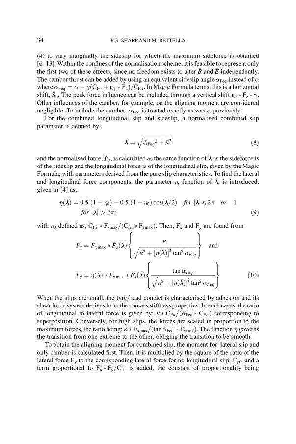
(4) to vary marginally the sideslip for which the maximum sideforce is obtained

[6–13]. Within the confines of the normalisation scheme, it is feasible to represent only

the first two of these effects, since no freedom exists to alter �BB and �EE independently.

The camber thrust can be added by using an equivalent sideslip angle �Feq instead of �where �Feq ¼ �þ �ðCF� þ g1 � FzÞ=CF�. In Magic Formula terms, this is a horizontal

shift, Sh. The peak force influence can be included through a vertical shift g1 � Fz � �.

Other influences of the camber, for example, on the aligning moment are considered

negligible. To include the camber, �Feq is treated exactly as was � previously.

For the combined longitudinal slip and sideslip, a normalised combined slip

parameter is defined by:

�� ¼ffiffiffiffiffiffiffiffiffiffiffiffiffiffiffiffiffiffiffiffiffi��Feq

2 þ ��2

qð8Þ

and the normalised force, �FFs, is calculated as the same function of �� as the sideforce is

of the sideslip and the longitudinal force is of the longitudinal slip, given by the Magic

Formula, with parameters derived from the pure slip characteristics. To find the lateral

and longitudinal force components, the parameter �, function of ��, is introduced,

given in [4] as:

�ð ��Þ ¼ 0:5:ð1 þ �0Þ 0:5:ð1 �0Þ cosð ��=2Þ for j ��j42� or 1

for j ��j > 2� : ð9Þ

with �0 defined as, Cf� � Fxmax=ðCf� � FymaxÞ. Then, Fx and Fy are found from:

Fx ¼ Fx max � �FFsð��Þ�ffiffiffiffiffiffiffiffiffiffiffiffiffiffiffiffiffiffiffiffiffiffiffiffiffiffiffiffiffiffiffiffiffiffiffiffiffiffiffiffiffiffi

�2 þ ½�ð��Þ�2 tan2 �Feq

q8><>:

9>=>; and

Fy ¼ �ð ��Þ � Fy max � �FFsð��Þtan�Feqffiffiffiffiffiffiffiffiffiffiffiffiffiffiffiffiffiffiffiffiffiffiffiffiffiffiffiffiffiffiffiffiffiffiffiffiffiffiffiffiffiffi

�2 þ ½�ð��Þ�2 tan2 �Feq

q8><>:

9>=>; ð10Þ

When the slips are small, the tyre=road contact is characterised by adhesion and its

shear force system derives from the carcass stiffness properties. In such cases, the ratio

of longitudinal to lateral force is given by: � � CF�=ð�Feq � CF�Þ corresponding to

superposition. Conversely, for high slips, the forces are scaled in proportion to the

maximum forces, the ratio being: � � Fxmax=ðtan�Feq � FymaxÞ. The function � governs

the transition from one extreme to the other, obliging the transition to be smooth.

To obtain the aligning moment for combined slip, the moment for lateral slip and

only camber is calculated first. Then, it is multiplied by the square of the ratio of the

lateral force Fy to the corresponding lateral force for no longitudinal slip, Fy0, and a

term proportional to Fx � Fy=Cf� is added, the constant of proportionality being


found by trial and error [10]. The force ratio term describes the process by which the

increasing longitudinal slip causes sliding from the rear of the contact patch, ensuring

that the forces there are primarily longitudinal rather than lateral and diminishing the

aligning moment correspondingly. The added term accounts for carcass compliances

[10] which lead (1) to the lateral force deforming the tyre laterally, giving rise to a

moment from the longitudinal force; and (2) to the longitudinal force influencing the

load distribution through the contact length and thereby the moment arising from

lateral forces. Division by the cornering stiffness accommodates in a simple way

changes in the carcass stiffnesses with loading. As the load increases, so does the

cornering stiffness and the lateral stiffness, until the carcass buckles, after which the

reverse process occurs.2

3. NORMALISED PARAMETER TREATMENT OF SHEAR FORCE

AND MOMENT DATA

3.1. Data Summary

The coefficient values for the nominal tyre from [6] relied upon, converted into SI

units from the original, are given in Table 1.

Secondary coefficients from [6] are sufficient to define the camber stiffnesses

for each standard load and the main influence of the camber on the sideforce peak

is expressed there in the relationship Sv¼ 0.848 � Fz � � (0.848, called g1 above, is

the coefficient a11 in [6] converted into SI units). The camber stiffnesses for the

nominal tyre are 648.3, 1780.2, 3341.9 and 5107.7 N=rad for 2, 4, 6 and 8 kN load,

respectively.

The preferred relationships giving the primary coefficients as functions of tyre load

are:

D ¼ a1 � F2z þ a2 � Fz;

BCD ¼ a3 � sinð2 � atanðFz=a4ÞÞ for the sideforce; ðthis is CF�Þ3

BCD ¼ fFzða3 � Fz þ a4Þg= expða5 � FzÞ for longitudinal force and

self aligning moment; ðthese are CF� and CM�ÞCF� ¼ a6 � F2

z þ a7 � Fz; ð11Þ

�p and �p are linearly related to the wheel load.

�p ¼ 0:13 6:5e 6 � Fz and �p ¼ 0:0786 þ 1:657e 5 � Fz: ð12Þ2 In numerical trials, this term has been found not to make a useful contribution, so the coefficient has been

set to zero.3 This is revised from the original in [6] and can be found in [7] and later versions of the formula.

TYRE SHEAR FORCE 35

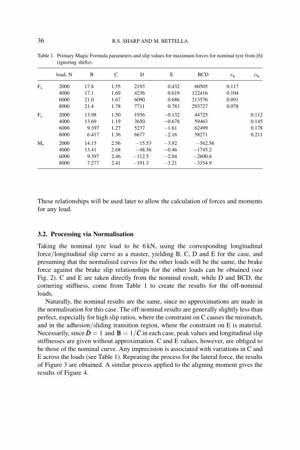
These relationships will be used later to allow the calculation of forces and moments

for any load.

3.2. Processing via Normalisation

Taking the nominal tyre load to be 6 kN, using the corresponding longitudinal

force=longitudinal slip curve as a master, yielding B, C, D and E for the case, and

presuming that the normalised curves for the other loads will be the same, the brake

force against the brake slip relationships for the other loads can be obtained (see

Fig. 2). C and E are taken directly from the nominal result, while D and BCD, the

cornering stiffness, come from Table 1 to create the results for the off-nominal

loads.

Naturally, the nominal results are the same, since no approximations are made in

the normalisation for this case. The off-nominal results are generally slightly less than

perfect, especially for high slip ratios, where the constraint on C causes the mismatch,

and in the adhesion=sliding transition region, where the constraint on E is material.

Necessarily, since �DD ¼ 1 and BB ¼ 1=�CC in each case, peak values and longitudinal slip

stiffnesses are given without approximation. C and E values, however, are obliged to

be those of the nominal curve. Any imprecision is associated with variations in C and

E across the loads (see Table 1). Repeating the process for the lateral force, the results

of Figure 3 are obtained. A similar process applied to the aligning moment gives the

results of Figure 4.

Table 1. Primary Magic Formula parameters and slip values for maximum forces for nominal tyre from [6]

(ignoring shifts).

load, N B C D E BCD �p �p

Fx 2000 17.8 1.55 2193 0.432 60505 0.117

4000 17.1 1.69 4236 0.619 122416 0.104

6000 21.0 1.67 6090 0.686 213576 0.091

8000 21.4 1.78 7711 0.783 293727 0.078

Fy 2000 13.98 1.50 1936 0.132 44725 0.112

4000 13.69 1.19 3650 0.678 59463 0.145

6000 9.397 1.27 5237 1.61 62499 0.178

8000 6.417 1.36 6677 2.16 58271 0.211

Mz 2000 14.15 2.56 15.53 3.92 562.56

4000 13.41 2.68 48.56 0.46 1745.2

6000 9.397 2.46 112.5 2.04 2600.6

8000 7.277 2.41 191.3 3.21 3354.9


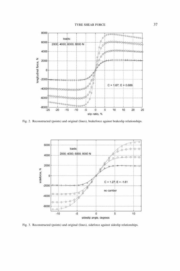
Fig. 2. Reconstructed (points) and original (lines), brakeforce against brakeslip relationships.

Fig. 3. Reconstructed (points) and original (lines), sideforce against sideslip relationships.

TYRE SHEAR FORCE 37

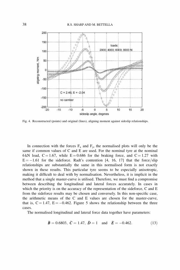
In connection with the forces Fx and Fy, the normalised plots will only be the

same if common values of C and E are used. For the nominal tyre at the nominal

6 kN load, C¼ 1.67, while E¼ 0.686 for the braking force, and C¼ 1.27 with

E¼1.61 for the sideforce. Radt’s contention [4, 16, 17] that the force=slip

relationships are substantially the same in this normalised form is not exactly

shown in these results. This particular tyre seems to be especially anisotropic,

making it difficult to deal with by normalisation. Nevertheless, it is implicit in the

method that a single master-curve is utilised. Therefore, we must find a compromise

between describing the longitudinal and lateral forces accurately. In cases in

which the priority is on the accuracy of the representation of the sideforce, C and E

from the sideforce results may be chosen and conversely. In this non-specific case,

the arithmetic means of the C and E values are chosen for the master-curve,

that is, C¼ 1.47, E¼0.462. Figure 5 shows the relationship between the three

cases.

The normalised longitudinal and lateral force data together have parameters:

�BB ¼ 0:6803; �CC ¼ 1:47; �DD ¼ 1 and �EE ¼ 0:462: ð13Þ

Fig. 4. Reconstructed (points) and original (lines), aligning moment against sideslip relationships.


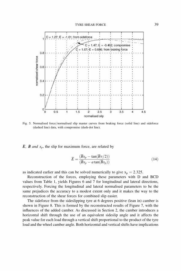
�EE; �BB and xp, the slip for maximum force, are related by

E ¼ ðBxp tanðB�=2ÞÞðBxp a tanðBxpÞÞ

ð14Þ

as indicated earlier and this can be solved numerically to give xp ¼ 2:325.

Reconstruction of the forces, employing these parameters with D and BCD

values from Table 1, yields Figures 6 and 7 for longitudinal and lateral directions,

respectively. Forcing the longitudinal and lateral normalised parameters to be the

same prejudices the accuracy to a modest extent only and it makes the way to the

reconstruction of the shear forces for combined slip easier.

The sideforce from the sideslipping tyre at 6 degrees positive (lean in) camber is

shown in Figure 8. This is formed by the reconstructed results of Figure 7, with the

influences of the added camber. As discussed in Section 2, the camber introduces a

horizontal shift through the use of an equivalent sideslip angle and it affects the

peak value for each load through a vertical shift proportional to the product of the tyre

load and the wheel camber angle. Both horizontal and vertical shifts have implications

Fig. 5. Normalised force=normalised slip master curves from braking force (solid line) and sideforce

(dashed line) data, with compromise (dash-dot line).

TYRE SHEAR FORCE 39

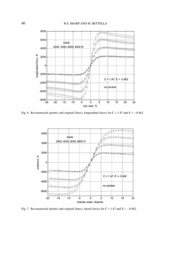
Fig. 6. Reconstructed (points) and original (lines), longitudinal forces for C¼ 1.47 and E¼0.462.

Fig. 7. Reconstructed (points) and original (lines), lateral forces for C¼ 1.47 and E¼0.462.


for the camber stiffness, which we take to be known from the measurements made.

The coefficient g1¼ 0.848, see Section 2, is also taken as known, either by

measurement or a priori knowledge. Then, the horizontal shift implied by converting

the sideslip into an equivalent sideslip including camber is designed to give the

correct tyre camber stiffnesses. The slip angle increment corresponding to unit

camber angle turns out to be:

ðCF� þ g1 � FzÞ=CF�: ð15Þ

Other influences of the camber on the sideforce and on the aligning moment included

in the full Magic Formula [13] are considered insignificant in the present context. A

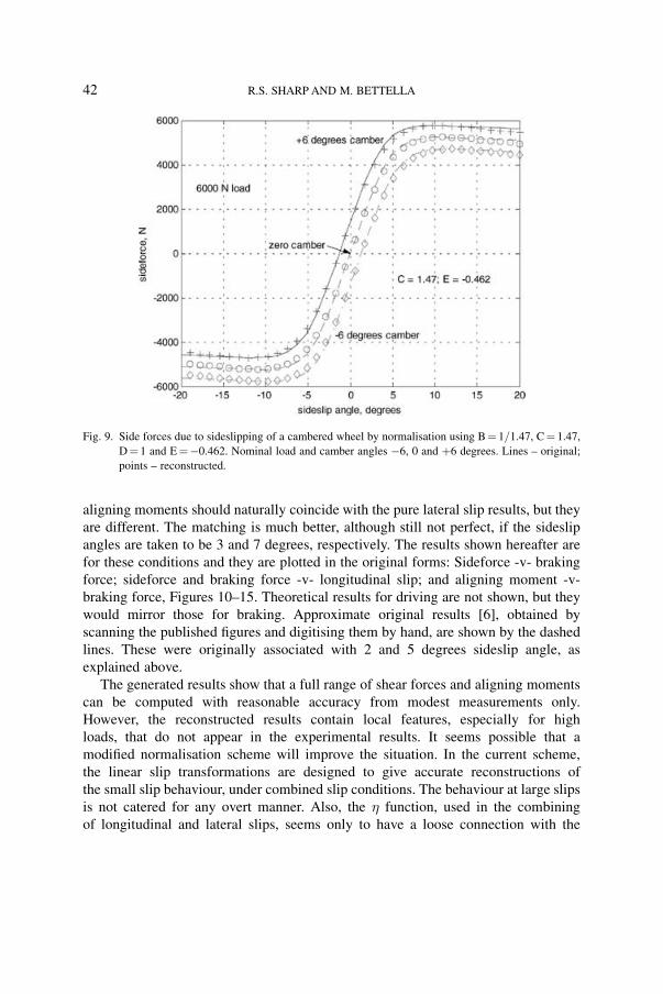
further illustration of the influence of the camber is given in Figure 9, treating the

nominal load and camber angles of 6, 0 and þ6 degrees.

With respect to the comparison of forces and moments under combined slip against

the original measured results [6], a difficulty arises due to certain inconsistencies in

that data. Force and moment results are given for longitudinal slip sweeps at fixed

sideslip angles quoted as 2 and 5 degrees. At zero longitudinal slip, the sideforces and

Fig. 8. Side forces due to sideslipping of a cambered wheel by normalisation using B¼ 1=1.47, C¼ 1.47,

D¼ 1 and E¼0.462. The influences of camber included are (1) through a horizontal shift of the

sideslip ðCF� þ g1 � FzÞ�=CF�; and (2) through a vertical shift g1 �Fz � �. Lines – original; points –

reconstructed.

TYRE SHEAR FORCE 41

aligning moments should naturally coincide with the pure lateral slip results, but they

are different. The matching is much better, although still not perfect, if the sideslip

angles are taken to be 3 and 7 degrees, respectively. The results shown hereafter are

for these conditions and they are plotted in the original forms: Sideforce -v- braking

force; sideforce and braking force -v- longitudinal slip; and aligning moment -v-

braking force, Figures 10–15. Theoretical results for driving are not shown, but they

would mirror those for braking. Approximate original results [6], obtained by

scanning the published figures and digitising them by hand, are shown by the dashed

lines. These were originally associated with 2 and 5 degrees sideslip angle, as

explained above.

The generated results show that a full range of shear forces and aligning moments

can be computed with reasonable accuracy from modest measurements only.

However, the reconstructed results contain local features, especially for high

loads, that do not appear in the experimental results. It seems possible that a

modified normalisation scheme will improve the situation. In the current scheme,

the linear slip transformations are designed to give accurate reconstructions of

the small slip behaviour, under combined slip conditions. The behaviour at large slips

is not catered for any overt manner. Also, the � function, used in the combining

of longitudinal and lateral slips, seems only to have a loose connection with the

Fig. 9. Side forces due to sideslipping of a cambered wheel by normalisation using B¼ 1=1.47, C¼ 1.47,

D¼ 1 and E¼0.462. Nominal load and camber angles 6, 0 and þ6 degrees. Lines – original;

points – reconstructed.


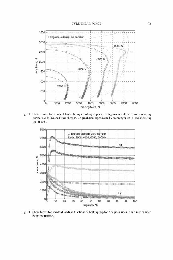
Fig. 10. Shear forces for standard loads through braking slip with 3 degrees sideslip at zero camber, by

normalisation. Dashed lines show the original data, reproduced by scanning from [6] and digitising

the images.

Fig. 11. Shear forces for standard loads as functions of braking slip for 3 degrees sideslip and zero camber,

by normalisation.

TYRE SHEAR FORCE 43

Fig. 12. Aligning moment and longitudinal force for standard loads as functions of braking slip for 3

degrees sideslip and zero camber, by normalisation. Dashed lines show the original data,

reproduced by scanning from [6] and digitising the images.

Fig. 13. Shear forces for standard loads through a complete range of braking slips with 7 degrees sideslip at

zero camber, by normalisation. Dashed lines show the original data, reproduced by scanning from

[6] and digitising the images.


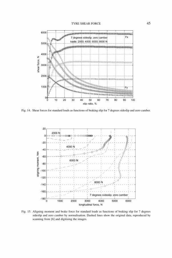
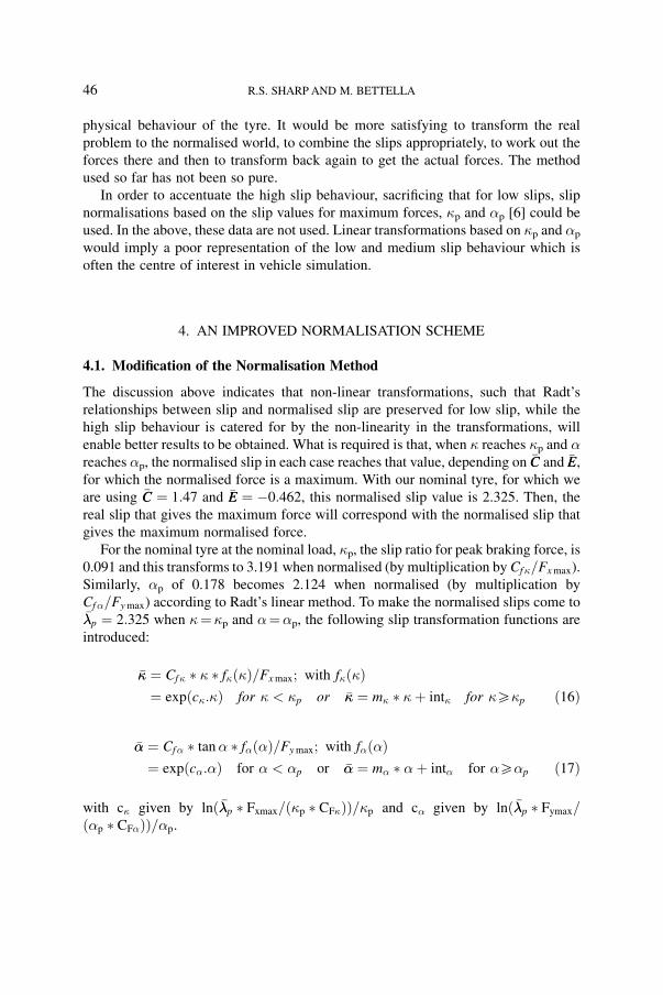
Fig. 14. Shear forces for standard loads as functions of braking slip for 7 degrees sideslip and zero camber.

Fig. 15. Aligning moment and brake force for standard loads as functions of braking slip for 7 degrees

sideslip and zero camber by normalisation. Dashed lines show the original data, reproduced by

scanning from [6] and digitising the images.

TYRE SHEAR FORCE 45

physical behaviour of the tyre. It would be more satisfying to transform the real

problem to the normalised world, to combine the slips appropriately, to work out the

forces there and then to transform back again to get the actual forces. The method

used so far has not been so pure.

In order to accentuate the high slip behaviour, sacrificing that for low slips, slip

normalisations based on the slip values for maximum forces, �p and �p [6] could be

used. In the above, these data are not used. Linear transformations based on �p and �p

would imply a poor representation of the low and medium slip behaviour which is

often the centre of interest in vehicle simulation.

4. AN IMPROVED NORMALISATION SCHEME

4.1. Modification of the Normalisation Method

The discussion above indicates that non-linear transformations, such that Radt’s

relationships between slip and normalised slip are preserved for low slip, while the

high slip behaviour is catered for by the non-linearity in the transformations, will

enable better results to be obtained. What is required is that, when � reaches �p and �reaches �p, the normalised slip in each case reaches that value, depending on �CC and �EE,

for which the normalised force is a maximum. With our nominal tyre, for which we

are using �CC ¼ 1:47 and �EE ¼ 0:462, this normalised slip value is 2.325. Then, the

real slip that gives the maximum force will correspond with the normalised slip that

gives the maximum normalised force.

For the nominal tyre at the nominal load, �p, the slip ratio for peak braking force, is

0.091 and this transforms to 3.191 when normalised (by multiplication by Cf�=Fx max).

Similarly, �p of 0.178 becomes 2.124 when normalised (by multiplication by

Cf�=Fy max) according to Radt’s linear method. To make the normalised slips come to��p ¼ 2:325 when �¼�p and �¼�p, the following slip transformation functions are

introduced:

�� ¼ Cf� � � � f�ð�Þ=Fx max; with f�ð�Þ¼ expðc�:�Þ for � < �p or �� ¼ m� � �þ int� for �5�p ð16Þ

�� ¼ Cf� � tan� � f�ð�Þ=Fy max; with f�ð�Þ¼ expðc�:�Þ for � < �p or �� ¼ m� � �þ int� for �5�p ð17Þ

with c� given by lnð��p � Fxmax=ð�p � CF�ÞÞ=�p and c� given by lnð��p � Fymax=ð�p � CF�ÞÞ=�p.


For continuity of both value and slope of f� and f� through �p and �p, it can be

shown that:

m� ¼ CF�ð1 þ c� � �pÞ expðc� � �pÞ=Fx max and

int� ¼ ðCF� expðc� � �pÞ=Fx max m�Þ�p ð18Þ

and similarly:

m� ¼ CF�ð1 þ c� � �pÞ expðc� � �pÞ=Fy max and

int� ¼ ðCF� expðc� � �pÞ=Fy max m�Þ�p ð19Þ

With these non-linear relationships between slip and normalised slip, it can be

expected that the good small slip behaviour of Radt’s method remains, but that

longitudinal and lateral slips exert equal influence in the normalised world, when the

slips are sufficient to saturate the tyre shear force. A determination of the normalised

shear force on the basis of the normalised resultant slip can be expected to deal fairly

between longitudinal and lateral and a resolution of the normalised shear force

through reference to the normalised slip components can be expected to be

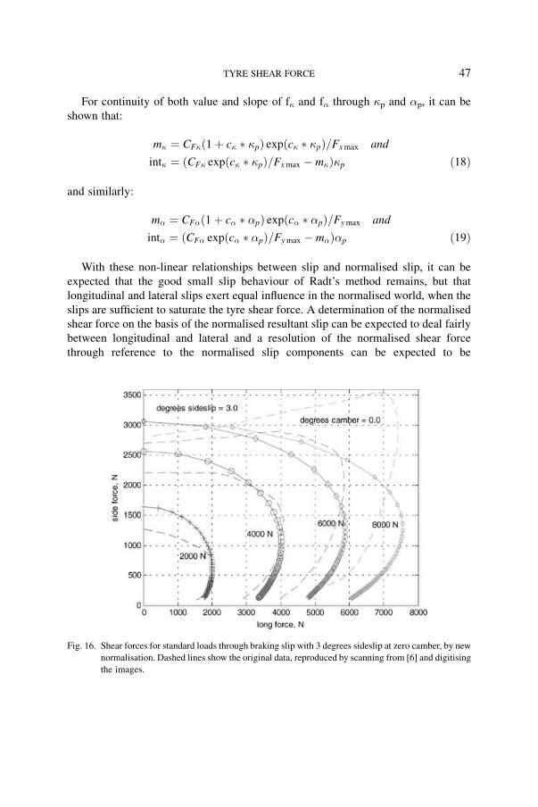
Fig. 16. Shear forces for standard loads through braking slip with 3 degrees sideslip at zero camber, by new

normalisation. Dashed lines show the original data, reproduced by scanning from [6] and digitising

the images.

TYRE SHEAR FORCE 47

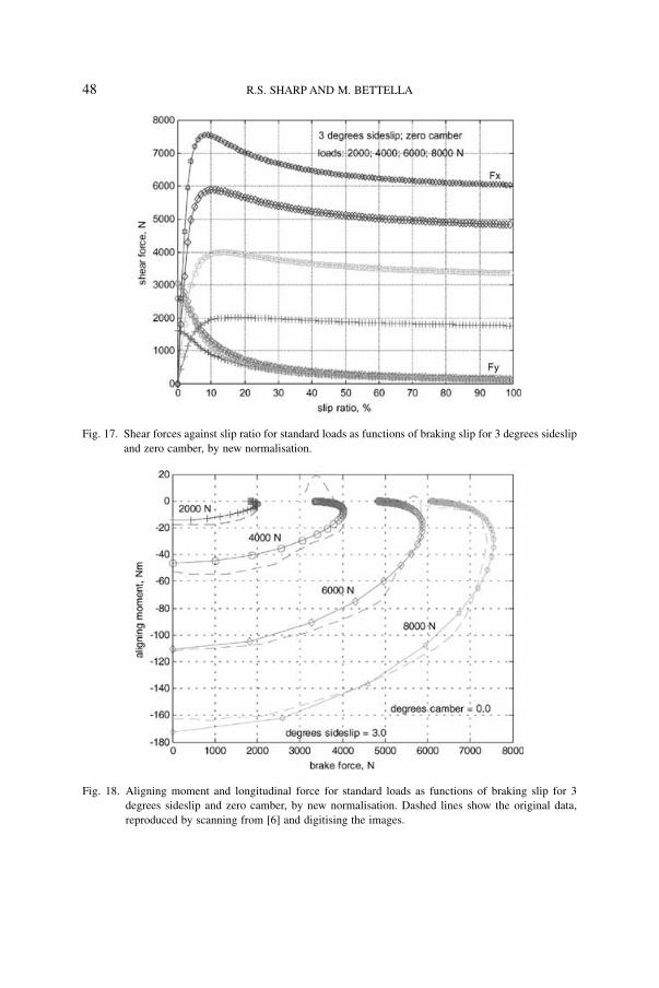
Fig. 17. Shear forces against slip ratio for standard loads as functions of braking slip for 3 degrees sideslip

and zero camber, by new normalisation.


degrees sideslip and zero camber, by new normalisation. Dashed lines show the original data,



reasonable. The somewhat arbitrary function, �, is no longer needed. Consequently,

the normalised force is obtained as:

�FFs ¼ �FFsð��Þ with �FFx ¼ �� FFs=�� and �FFy ¼ �� FFs=��: ð20Þ

Then, de-normalising the force components by reversing the original, simple

normalisation yields:

Fx ¼ Fx max � �FFx and Fy ¼ Fy max � �FFy ð21Þ

4.2. Results from the New Scheme

Repeating the trials that gave rise to the results of Figures 10–15 with the new

algorithm, Figures 16–21 are obtained.

The non-linear longitudinal slip transformation used in the calculations is shown in

Figure 22. The slope at the origin, in each case, is given by the ratio: slip stiffness to

peak force. Then the exponent in the transformation relationship changes that slope

until the slip � reaches �p. For larger slips, the relationship is linear. A corresponding

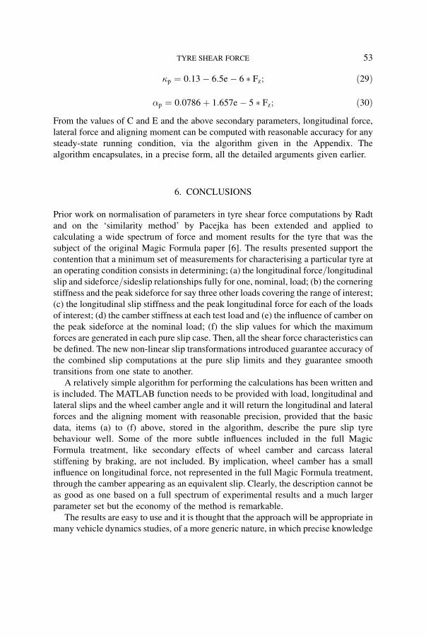
set of curves belongs to the lateral slip transformations (Fig. 23).

Fig. 19. Shear forces for standard loads through a complete range of braking slips with 7 degrees sideslip at

zero camber, by new normalisation. Dashed lines show the original data, reproduced by scanning

from [6] and digitising the images.

TYRE SHEAR FORCE 49

Fig. 20. Shear forces against slip ratio for standard loads as functions of braking slip for 7 degrees sideslip

and zero camber, by new normalisation.


degrees sideslip and zero camber, by new normalisation. Dashed lines show the original data,



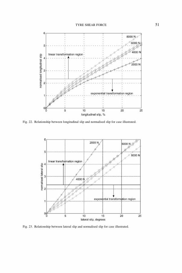
Fig. 22. Relationship between longitudinal slip and normalised slip for case illustrated.

Fig. 23. Relationship between lateral slip and normalised slip for case illustrated.

TYRE SHEAR FORCE 51

5. GENERAL APPLICATION

To see the general application of the process, let us suppose the following scenario: The

nominal load of a tyre is selected, slightly biased towards the high end of its load range,

since it is more important to compute accurately the large forces, when the tyre loading

is relatively high. At the nominal load, a sideslip sweep is conducted and the sideforce

and the aligning moment are measured. Similarly, a longitudinal slip sweep at straight

running is conducted. Any offsets due to rolling resistance and tyre imperfections are

removed from the results. B, C, D and E Magic Formula primary parameters are found

for each of longitudinal force, lateral force and aligning moment. In general, C and E

values for the two forces will be different and, since it is necessary to select one value

of C and one of E only, in order to deal with combined slip effectively, it may be

preferable to select C and E ahead of testing, based on prior knowledge, and to restrict

the testing to small and moderate slip levels. Three other loads are selected and peak

force and moment values and stiffnesses (force and moment derivatives for small slips)

are determined. The slip values for which the forces peak are noted in each case. For

each of the four loads, the camber angle is set to 5 degrees say and the camber thrust is

measured for no sideslip. Also, the peak force is found by performing a local sideslip

sweep near to the peak force value. These measurements with camber give the camber

stiffnesses for each of the four loads and the influence of the camber angle on the peak

lateral force. The measurement database is now complete.

Values for C and E for the forces are fixed first, possibly by compromise between

longitudinal and lateral results or by presumption as mentioned above. C and E values

for the aligning moment at the nominal load are adopted as standard. Then, to enable

the calculation of the other required parameters for any load, secondary parameters

which best describe the primary parameters in terms of load are derived, using the

equations of Section 2. For the data in Table 1 and the camber stiffnesses given, the

following results are obtained:

CF� ¼ fFzð0:00377 � Fz þ 23:731Þg= expð4:744e 5 � FzÞ; ð22Þ

CF� ¼ 63306 � sinð2 � atanðFz=5094ÞÞ; ð23Þ

CM� ¼ fFzð2:135e 4 � Fz 0:0051Þg= expð1:76e 4 � FzÞ; ð24Þ

CF� ¼ 4:861e 5 � Fz2 þ 0:2537 � Fz; ð25Þ

D for Fx ¼ 2:347e 5 � Fz2 þ 1:153 � Fz; ð26Þ

D for Fy ¼ 2:035e 5 � Fz2 þ 0:9966 � Fz; ð27Þ

D for Mz ¼ 2:804e 6 � Fz2 þ 0:001551 � Fz; ð28Þ


�p ¼ 0:13 6:5e 6 � Fz; ð29Þ

�p ¼ 0:0786 þ 1:657e 5 � Fz; ð30Þ

From the values of C and E and the above secondary parameters, longitudinal force,

lateral force and aligning moment can be computed with reasonable accuracy for any

steady-state running condition, via the algorithm given in the Appendix. The

algorithm encapsulates, in a precise form, all the detailed arguments given earlier.

6. CONCLUSIONS

Prior work on normalisation of parameters in tyre shear force computations by Radt

and on the ‘similarity method’ by Pacejka has been extended and applied to

calculating a wide spectrum of force and moment results for the tyre that was the

subject of the original Magic Formula paper [6]. The results presented support the

contention that a minimum set of measurements for characterising a particular tyre at

an operating condition consists in determining; (a) the longitudinal force=longitudinal

slip and sideforce=sideslip relationships fully for one, nominal, load; (b) the cornering

stiffness and the peak sideforce for say three other loads covering the range of interest;

(c) the longitudinal slip stiffness and the peak longitudinal force for each of the loads

of interest; (d) the camber stiffness at each test load and (e) the influence of camber on

the peak sideforce at the nominal load; (f) the slip values for which the maximum

forces are generated in each pure slip case. Then, all the shear force characteristics can

be defined. The new non-linear slip transformations introduced guarantee accuracy of

the combined slip computations at the pure slip limits and they guarantee smooth

transitions from one state to another.

A relatively simple algorithm for performing the calculations has been written and

is included. The MATLAB function needs to be provided with load, longitudinal and

lateral slips and the wheel camber angle and it will return the longitudinal and lateral

forces and the aligning moment with reasonable precision, provided that the basic

data, items (a) to (f) above, stored in the algorithm, describe the pure slip tyre

behaviour well. Some of the more subtle influences included in the full Magic

Formula treatment, like secondary effects of wheel camber and carcass lateral

stiffening by braking, are not included. By implication, wheel camber has a small

influence on longitudinal force, not represented in the full Magic Formula treatment,

through the camber appearing as an equivalent slip. Clearly, the description cannot be

as good as one based on a full spectrum of experimental results and a much larger

parameter set but the economy of the method is remarkable.

The results are easy to use and it is thought that the approach will be appropriate in

many vehicle dynamics studies, of a more generic nature, in which precise knowledge

TYRE SHEAR FORCE 53

of tyre properties is unavailable and in which the results sought will be relatively

insensitive to variations in tyre force details.

A new notation has been contributed, with the intention to make the procedures

more easily understood. The algorithm can be seen to be short. Its computing time

will be short in comparison with many alternatives, although formal trials of this

aspect have not been made.

REFERENCES

1. Clark, S.K.: Mechanics of Pneumatic Tires. NBS Monograph 122, 2nd ed., 1981.

2. Wong, J.Y.: Theory of Ground Vehicles. Wiley, New York, 2nd ed., 1993.

3. Dixon, J.C.: Tires, Suspension and Handling, SAE Inc., Warrendale, PA, 2nd ed., 1996.

4. Milliken, W.F. and Milliken, D.L.: Race Car Vehicle Dynamics. SAE Inc., Warrendale, PA, 1995.

5. Genta, G.: Motor Vehicle Dynamics: Modeling and Simulation. World Scientific Publishing,

Singapore, 1997.

6. Bakker, E., Nyborg, L. and Pacejka, H.B.: Tyre Modelling for Use in Vehicle Dynamics Studies. SAE

Paper 870421, 1987.

7. Bakker, E., Pacejka, H.B. and Lidner, L.: A New Tyre Model with Application in Vehicle Dynamics

Studies. Proc. 4th Int. Conf. Automotive Technologies, Monte Carlo, 1989, SAE paper 890087, 1989.

8. Pacejka, H.B. and Bakker, E.: The Magic Formula Tyre Model. Proc. 1st International Tyre

Colloquium, Delft, 1991. Vehicle System Dynamics 21 (Suppl.) (1991), pp. 1–18.

9. Van Oosten, J.J.M. and Bakker, E.: Determination of Magic Formula Parameters. Proc. 1st

International Tyre Colloquium, Delft, 1991. Vehicle System Dynamics 21 (Suppl.) (1991), pp. 19–29.

10. Pacejka, H.B. and Sharp, R.S.: Shear Force Generation by Pneumatic Tyres in Steady State Conditions:

a Review of Modelling Aspects. Vehicle System Dynamics 20 (1991), pp. 121–176.

11. Schuring, D.J., Pelz, W. and Pottinger, M.G.: The BNPS Model – an Automated Implementation of the

‘‘Magic Formula’’ Concept. Proc. IPC-7 Conf., Phoenix, AZ, 1993.

12. Bayle, P., Forissier, J.F. and Lafon, S.: A New Tyre Model for Vehicle Dynamic Simulations.

Automotive Technologies International, (1993), pp. 193–198.

13. Pacejka, H.B. and Besselink, I.J.M.: Magic Formula Tyre Model with Transient Properties. Proc. 2nd

International Tyre Colloquium, Berlin, 1997. Vehicle System Dynamics 27 (Suppl.) (1997),

pp. 234–249.

14. Bernard, J.E., Segel, L. and Wild, R.E.: Tire Shear Force Generation During Combined Steering and

Braking Maneuvers. SAE Paper 770852, 1977.

15. Allen, R.W. and Szostak, H.T.: Steady State and Transient Analysis of Ground Vehicle Handling, SAE

Paper 870495, 1987.

16. Radt, H.S. and Milliken, W.F.: Non-Dimensionalising Tyre Data for Vehicle Simulation. Road Vehicle

Handling. MEP, London, 1983, pp. 229–240.

17. Radt, H.S. and Glemming, D.A.: Normalization of Tire Force and Moment Data. Tire Science and

Technology, TSTCA 21(2) (1993), pp. 91–119.

18. Lugner, P. and Mittermayr, P.: A Measurement Based Tyre Characteristics Approximation. Proc.

1st International Tyre Colloquium, Delft, 1991. Vehicle System Dynamics 21 (Suppl.) (1991),

pp. 127–144.

19. Vehicle Dynamics Terminology. SAE Paper J670e. Society of Automotive Engineers, Warrendale,

PA, 1976.

20. Nakayama, Y. and Boucher, R.F.: Introduction to Fluid Mechanics. Arnold, London, 1999.


APPENDIX

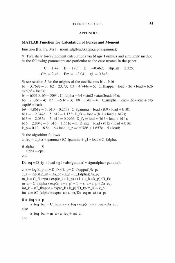
MATLAB Function for Calculation of Forces and Moment

function [Fx, Fy, Mz]¼ norm_alg(load,kappa,alpha,gamma);

% Tyre shear force=moment calculations via Magic Formula and similarity method

% the following parameters are particular to the case treated in the paper

C ¼ 1:47; B ¼ 1=C; E ¼ 0:462; slipm ¼ 2:325;

Cm ¼ 2:46; Em ¼ 2:04; g1 ¼ 0:848;

% see section 5 for the origins of the coefficients b1. . .b16

b1¼ 3.769e 3; b2¼ 23.73; b3¼ 4.744e 5; C_fkappa¼ load � (b1 � loadþ b2)/

exp(b3 � load);

b4¼ 63310; b5¼ 5094; C_falpha¼ b4 � sin(2 � atan(load=b5));

b6¼ 2.135e 4; b7¼5.1e 3; b8¼ 1.76e 4; C_malpha¼ load� (b6� loadþ b7)/

exp(b8� load);

b9¼ 4.861e 5; b10¼ 0.2537; C_fgamma¼ load � (b9 � loadþ b10);

b11¼2.347e 5; b12¼ 1.153; D_fx¼ load � (b11 � loadþ b12);

b13¼2.035e 5; b14¼ 0.9966; D_fy¼ load � (b13 � loadþ b14);

b15¼ 2.804e 6; b16¼ 1.551e 3; D_mz¼ load � (b15 � loadþ b16);

k_p¼ 0.13 6.5e 6 � load; a_p¼ 0.0786þ 1.657e 5 � load;

% the algorithm follows

a_feq¼ alphaþ gamma � (C_fgammaþ g1 � load)=C_falpha;

if alpha¼ ¼ 0

alpha¼ eps;

end

Da_eq¼D_fyþ load � g1 � abs(gamma) � sign(alpha � gamma);

c_k¼ log(slip_m �D_fx=(k_p �C_fkappa))=k_p;

c_a¼ log(slip_m �Da_eq=(a_p �C_falpha))=a_p;

m_k¼C_fkappa � exp(c_k � k_p) � (1þ c_k � k_p)=D_fx;

m_a¼C_falpha � exp(c_a � a_p) � (1þ c_a � a_p)=Da_eq;

int_k¼ (C_fkappa � exp(c_k � k_p)=D_fx-m_k) � k_p;

int_a¼ (C_falpha � exp(c_a � a_p)=Da_eq-m_a) � a_p;

if a_feq < a_p

a_feq_bar¼C_falpha � a_feq � exp(c_a � a_feq)=Da_eq;

else

a_feq_bar¼m_a � a_feqþ int_a;

end

TYRE SHEAR FORCE 55

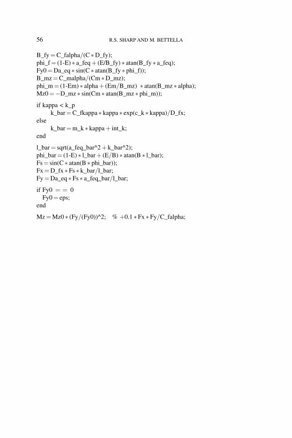
B_fy¼C_falpha=(C �D_fy);

phi_f¼ (1-E) � a_feqþ (E/B_fy) � atan(B_fy � a_feq);

Fy0¼Da_eq � sin(C � atan(B_fy � phi_f));

B_mz¼C_malpha=(Cm �D_mz);

phi_m¼ (1-Em) � alphaþ (Em=B_mz) � atan(B_mz � alpha);

Mz0¼D_mz � sin(Cm � atan(B_mz � phi_m));

if kappa < k_p

k_bar¼C_fkappa � kappa � exp(c_k � kappa)=D_fx;

else

k_bar¼m_k � kappaþ int_k;

end

l_bar¼ sqrt(a_feq_bar^2þ k_bar^2);

phi_bar¼ (1-E) � l_barþ (E=B) � atan(B � l_bar);

Fs¼ sin(C � atan(B � phi_bar));

Fx¼D_fx � Fs � k_bar=l_bar;

Fy¼Da_eq � Fs � a_feq_bar=l_bar;

if Fy0 ¼ ¼ 0

Fy0¼ eps;

end

Mz¼Mz0 � (Fy=(Fy0))^2; % þ0.1 � Fx � Fy=C_falpha;


tyre shear force and moment descriptions and the ‘‘magic

Documents