On the construction of a general numerical tyre shear force model

from limited data

R. S. Sharp* and M. Bettella**

*Department of Electrical and Electronic Engineering, Imperial College of Science,

Technology and Medicine, London SW7 2BT

**Jaguar Cars Engineering Centre, Whitley, Coventry CV3 4LF

Keywords: Tyre, shear force, Magic Formula, normalisation

Abstract: The extension of very limited tyre shear force and moment measured results to

allow the modelling and simulation of quite general motions of automobiles is discussed.

Relying on a recently devised algorithm, that has its basis in Magic Formula and parameter

normalization methods, processes are devised for determining the necessary parameter values

of the algorithm. The method is applied to each of two tyres, having substantially different

natures. Where data is lacking, fundamental knowledge of tyre mechanics is applied to the

problem of obtaining the best values. Results are included to demonstrate the effectiveness

of the processes. Data sets for the particular tyres treated and the algorithm itself are

included.

NOTATION

b1-b16; Magic Formula secondary parameters

Bm, Bx, By, C, Cfκ, Cfα, Cfγ ,Cm, Cmα, Dx, Dy, Dmz, E, Em; Magic Formula primary parameters

Cmz1, Cmz2, Cmz3, Emz1, Emz2, Emz3; polynomial coefficients of expressions for Cm and Em

;,, ECB normalised Magic Formula parameters

Fx, Fy, Mz; longitudinal force, lateral force and aligning moment from tyre

Fz; tyre load

g1; mean ratio of camber stiffness to tyre load

slip_m; normalized slip value for which normalized force is maximum

;, ακ longitudinal slip ratio and sideslip angle

κp, αp; slip ratio and slip angle for maximum shear force in pure slip

1 INTRODUCTION

In vehicle dynamics modelling, representing the tyre shear force system properly with respect

to the purposes of the activity is well known to be vital. Often, however, tyre shear force data

is sparse and it may be prohibitively expensive to obtain directly by measurement. It is

therefore of interest to consider the problem of creating a comprehensive shear force model

from the kind of limited data that often exists [1]. The objective is to use the data, such as it

is, to make a general model that will represent real tyre shear force and moment behaviour

with generic accuracy. It is also implied that any special tyre force characteristics that may

be of interest can be included in the model built, if success is achieved in the main objective.

Several standard vehicle dynamics simulation tests like constant radius turning, the

double lane change or the J-turn roll-over test are almost pure lateral tests. In such cases,

there is more value in a good representation of the lateral force, compared to the longitudinal

one. On the other hand, ma noeuvres dominated by braking or driving demand more accuracy

from the longitudinal force model, while braking in a turn, for example, requires longitudinal

and lateral to be weighted equally.

Recent research [2] has shown that pure slip longitudinal and lateral force data for

several tyre loads can be processed in such a way that combined slip forces are derivable

from them. A combination of the “Magic Formula” [3] and similarity or normalisation

methods [1, 4, 5], together with a new non-linear slip transformation were used. The slip

transformation allows both the low slip and high slip shear forces in combined longitudinal

and lateral slip to be represented with reasonable accuracy, with a guaranteed smooth

transition from braking to cornering. The method involves the adoption of a Magic Formula

master curve to represent both longitudinal and lateral forces. When both of these have been

measured, it is necessary to compromise between the two, in terms of the accuracy of

representation, or to deliberately favour one or the other through the choice of parameter

values. The more isotropic a particular tyre is, the less the compromise becomes.

Most commonly, existing data comes in the form of side force against slip angle and

aligning moment against slip angle for each of several loads, typically four in number [1, 6].

It is comparatively rare to find corresponding longitudinal force against slip ratio results,

partly because some tyre testing rigs are not equipped with braking or driving systems and

therefore they are not capable in this respect. Consequently, the present development is

aimed at taking side force and aligning moment data for several loads and deriving from them

the necessary coefficients to generate a whole spectrum of steady state shear force and

aligning moment characteristics. The coefficients are those of the algorithm, devised in

reference [2] and modified slightly below, which takes load, slip ratio, slip angle and camber

angle and gives back longitudinal force, lateral force and aligning moment.

In section 2, the starting data and the processing necessary to derive the coefficients

for one particular tyre are explained. A full set of coefficients is derived. In section 3, the

coefficients are used to compute combined slip force and moment results and these are

shown. In section 4, a second tyre data set is treated in a similar way and corresponding

results are given. Conclusions are drawn in section 5.

2 DATA AND PROCESSING FOR A RACE TYRE

The starting point is the data for a Goodyear F1 front tyre, 25.0 x 9.0 – 13 (of some years

ago) (given in reference [1], figure 2.46). Both side force and aligning moment data were

scanned and saved as bitmaps. The maps were then read into MATLAB, using “imread”

and sampled and digitized, using “ginput”. The side force data were then used to evaluate C

and E, presumed to be the same for each load [2], b4, b5, relating the cornering stiffness to the

load, and b13 and b14, relating the peak side force to the load. The relevant equations, from

reference [2], are:

)3().(

)2())/arctan(2sin(

)1())}]arctan((arctan{sin[

1413

54

bFbFD

DCBbFbC

BBEBCDF

zzy

yyzf

yyyyy

+=

==

−−=

α

ααα

The optimization routine “fminsearch” with a sum-of-squares-of-errors objective function

was used for this purpose. The original and reconstructed side force / slip angle results are

shown in Fig. 1.

Fig. 1 Original (solid lines) and reconstructed (dotted lines) side force data for Goodyear F1

front tyre, 25.0 x 9.0 – 13 from reference [1], with invariant C and E

Parameter values obtained in the error minimization are: C = 1.4125; E = 0.42922; b4 =

166303; b5 = 3826.8; b13 = -0.00012267; b14 = 1.96015. The reconstruction can be seen to be

of good quality.

The side force – load data is also used to derive a linear relationship between the slip

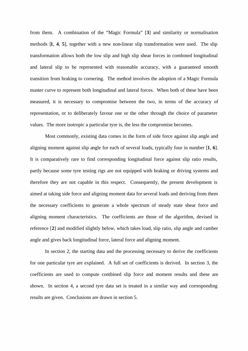
angle for maximum force and load. The former is obtained by solving the equation [2, 3, 5]:

)4()}arctan({

})2tan({

pypy

py

BB

CBE

αα

πα

−

−=

for pα for each load and fitting a straight line to the result. The values and the best fit

straight line, are shown in Fig. 2.

1500 2000 2500 3000 3500 4000 45000.08

0.09

0.1

0.11

0.12

0.13

0.14

0.15

0.16

tyre load, N

slip

ang

le fo

r pea

k fo

rce,

rad

best straight line fit values found from equation 4

Fig. 2 Values of pα from solving (4) given By, C and E for each of the four standard loads,

and its straight line fit: 054238.0.000019463.0 += zp Fα

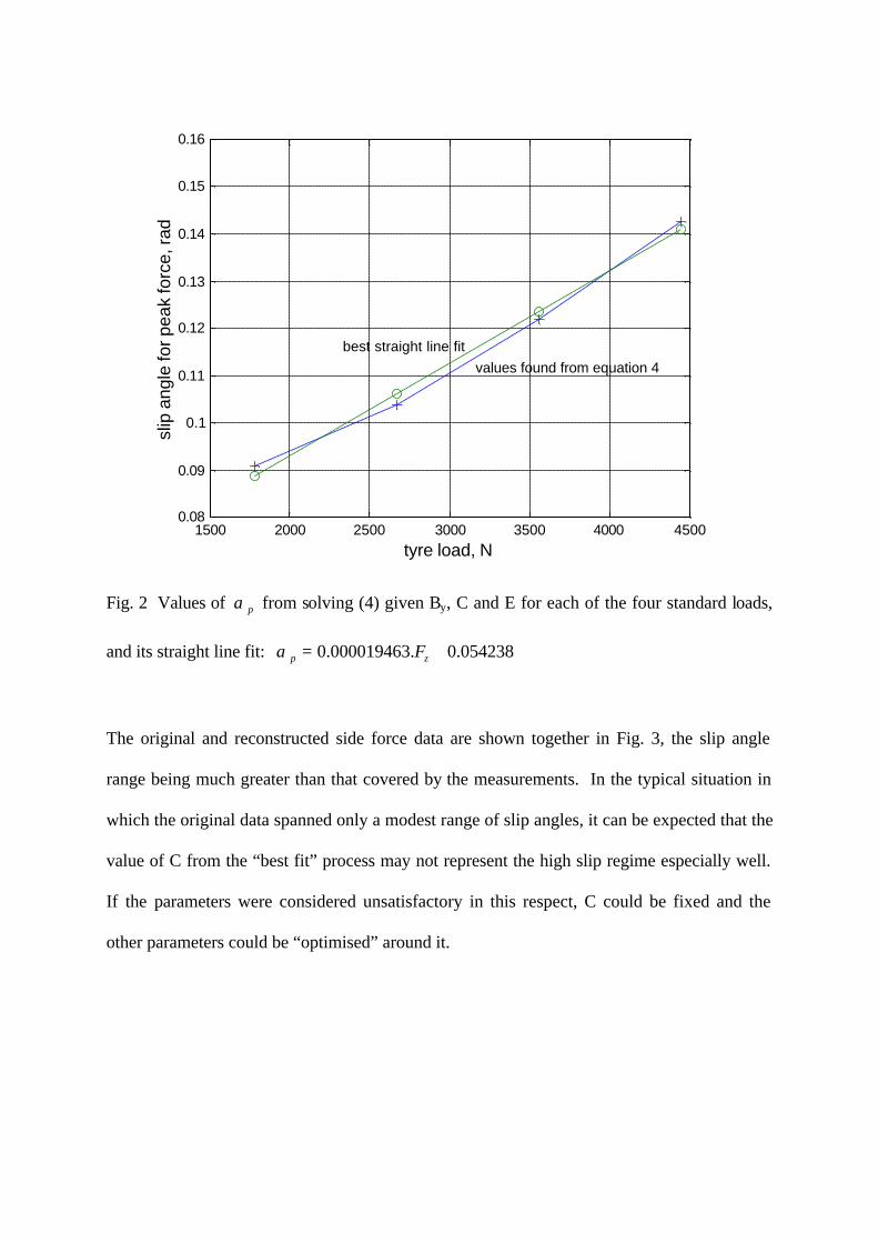
The original and reconstructed side force data are shown together in Fig. 3, the slip angle

range being much greater than that covered by the measurements. In the typical situation in

which the original data spanned only a modest range of slip angles, it can be expected that the

value of C from the “best fit” process may not represent the high slip regime especially well.

If the parameters were considered unsatisfactory in this respect, C could be fixed and the

other parameters could be “optimised” around it.

-15 -10 -5 0 5 10 15-8000

-6000

-4000

-2000

0

2000

4000

6000

8000

sideslip angle, degrees

side

forc

e, N

original datano camber

loads:1780; 2670; 3560; 4450 N

Fig. 3 Side forces as functions of sideslip angle using coefficients from fitting process and

showing original data from reference [1]

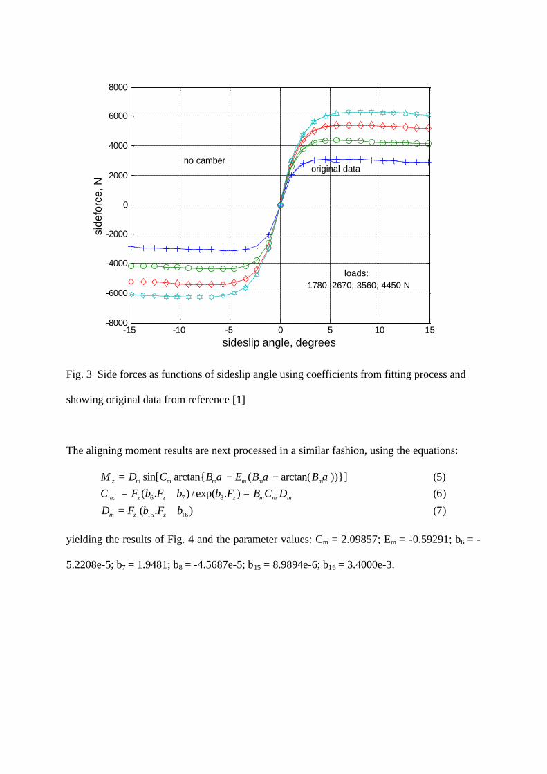
The aligning moment results are next processed in a similar fashion, using the equations:

)7().(

)6().exp(/).()5())}]arctan((arctan{sin[

1615

876

bFbFD

DCBFbbFbFCBBEBCDM

zzm

mmmzzzm

mmmmmmz

+=

=+=−−=

α

ααα

yielding the results of Fig. 4 and the parameter values: Cm = 2.09857; Em = -0.59291; b6 = -

5.2208e-5; b7 = 1.9481; b8 = -4.5687e-5; b15 = 8.9894e-6; b16 = 3.4000e-3.

0 0.02 0.04 0.06 0.08 0.1 0.12-50

0

50

100

150

200

slip angle, rad

alig

ning

mom

ent,

Nm

1780 N2670 N

3560 N

4450 N

Fig. 4 Original (solid lines) and reconstructed (dotted lines) aligning moment data for

Goodyear F1 front tyre, 25.0 x 9.0 – 13 from reference [1], with Cm = 2.099 and Em.= -0.5929

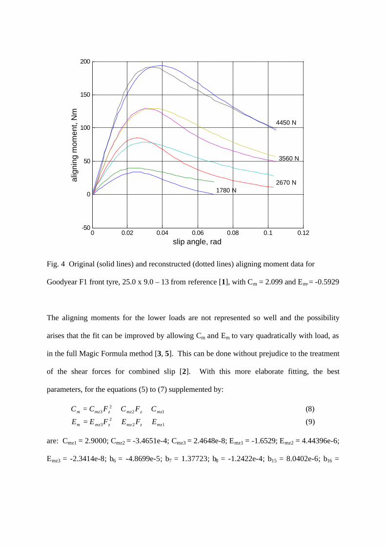
The aligning moments for the lower loads are not represented so well and the possibility

arises that the fit can be improved by allowing Cm and Em to vary quadratically with load, as

in the full Magic Formula method [3, 5]. This can be done without prejudice to the treatment

of the shear forces for combined slip [2]. With this more elaborate fitting, the best

parameters, for the equations (5) to (7) supplemented by:

)9(

)8(

122

3

122

3

mzzmzzmzm

mzzmzzmzm

EFEFEE

CFCFCC

++=

++=

are: Cmz1 = 2.9000; Cmz2 = -3.4651e-4; Cmz3 = 2.4648e-8; Emz1 = -1.6529; Emz2 = 4.44396e-6;

Emz3 = -2.3414e-8; b6 = -4.8699e-5; b7 = 1.37723; b8 = -1.2422e-4; b15 = 8.0402e-6; b16 =

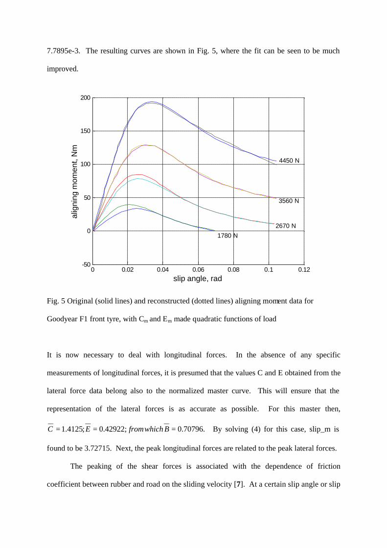
7.7895e-3. The resulting curves are shown in Fig. 5, where the fit can be seen to be much

improved.

0 0.02 0.04 0.06 0.08 0.1 0.12-50

0

50

100

150

200

slip angle, rad

alig

ning

mom

ent,

Nm

1780 N

2670 N

3560 N

4450 N

Fig. 5 Original (solid lines) and reconstructed (dotted lines) aligning moment data for

Goodyear F1 front tyre, with Cm and Em made quadratic functions of load

It is now necessary to deal with longitudinal forces. In the absence of any specific

measurements of longitudinal forces, it is presumed that the values C and E obtained from the

lateral force data belong also to the normalized master curve. This will ensure that the

representation of the lateral forces is as accurate as possible. For this master then,

.70796.0;42922.0;4125.1 === BwhichfromEC By solving (4) for this case, slip_m is

found to be 3.72715. Next, the peak longitudinal forces are related to the peak lateral forces.

The peaking of the shear forces is associated with the dependence of friction

coefficient between rubber and road on the sliding velocity [7]. At a certain slip angle or slip

ratio, the sliding of the rubber tread elements across the road is such that the shear force is

maximized. In the limit when the tyre load is low, the contact between tyre and ground

becomes line contact and the optimum sliding condition longitudinally will be the same as

that laterally. The peak forces will consequently be the same, which implies that b12, for the

longitudinal force, will be equal to b14, for the lateral force with value 1.96015, which value,

incidentally, represents the maximum coefficient of friction between the tyre rubber and the

ground in the rig test conditions. As the tyre load increases and the contact lengthens, the

greater stiffness of the tread base longitudinally will motivate the tread rubber elements

towards the same sliding velocity more in longitudinal slip than in lateral slip. The

consequence of this is that the longitudinal force peak will be higher and the peak will be

sharper [8]. It is estimated here that the peak longitudinal force will be 10% higher than the

peak lateral force for the highest of the standard loads, 4450 N, which implies that b11 = -

9.0889e-5.

It is also characteristic of the peak longitudinal forces that they occur at the same slip

ratio, typically κp = 0.13, irrespective of load. Presuming the same C and E values (1.4125

and 0.42922 respectively) for lateral force, longitudinal force and master curve and knowing

κp allows the calculation of Bx from (4). Bx must be constant, since C, E and κp are load

invariant. This implies that Cfκ, which is Bx.C.Dx varies with load exactly as does Dx, which

implies that b3 = 0, b1 = Bx.C.b11 and b2 = Bx.C.b12. Fig. 6 shows the resulting longitudinal

forces as functions of slip ratio. Now, we are missing only b9, b10 and g1 – all to do with

wheel camber.

-25 -20 -15 -10 -5 0 5 10 15 20 25-8000

-6000

-4000

-2000

0

2000

4000

6000

8000

slip ratio, %

long

itudi

nal f

orce

, N

C = 1.4125; E = 0.42922

loads:1780; 2670; 3560; 4450 N

Fig. 6 Longitudinal forces as functions of slip ratio, using selected parameter values

Camber is assumed to influence peak force according to (g1.Fz.γ). The topic is treated in

reference [1] at figures 2.25 and 2.26. 2.25 is for a fixed load, while 2.26 is for each of four

loads. The force gain due to camber is very variable over load but taking the mean, g1 comes

to 0.75, not so different from the value of 0.848 given in reference [8]. b9 and b10 relate the

load to the camber stiffness. Figures 2.28 and 2.29 of reference [1] apply. Also, in the limit

when the tyre becomes a thin disk, it can be expected that the camber thrust will be equal to

the wheel load multiplied by the tangent of the camber angle. (For such a thin disk brush

type tyre, from loaded free rolling, with straight contact line and no sideforce, imagine the

wheel to be cambered but not so much as to cause sliding in the contact region. Subsequent

rolling will maintain the straight contact line. What was previously the load on the tyre will

now be a force in the plane of the wheel. That force can be resolved into a vertical load equal

to the former load multiplied by the cosine of the camber angle and a camber thrust, which is

the former load multiplied by the sine of the camber angle. The ratio of camber thrust to load

is now the tangent of the camber angle). In the latter case, b9 would be zero while b10 would

be 1, whereas the experimental curves show non-linearity with load, consistent with b10 being

less than 1 and b9 being small but positive. To get a reasonable match with the non-linearity

in figure 2.28, we take b9 = 0.00005 and b10 = 0.5, compared with 0.00004861 and 0.2537

from reference [8].

3 COMBINED SLIP FORCE AND MOMENT RESULTS

These considerations yield a complete data set as follows:

C = 1.4125; B = 1/C; E = 0.42922; slip_m = 3.72715; g1 = 0.75;

Cm = Cmz1+Cmz2*Fz+Cmz3*Fz2 with Cmz1 = 2.9000; Cmz2 = -3.4651e-4; Cmz3 = 2.4648e-8;

Em = Emz1+Emz2*Fz+Emz3*Fz2 with Emz1 = -1.6529; Emz2 = 4.4396e-6; Emz3 = -2.3414e-8;

b1 = -0.0026058; b2 = 56.1982; b3 = 0;

b4 = 166303; b5 = 3826.8;

b6 = -4.8699e-5; b7 = 1.37723; b8 = -1.24221e-4;

b9 = 0.00005; b10 = 0.5;

b11 = -9.0889e-5; b12 = 1.96015;

b13 = -0.0001227; b14 = 1.96015;

b15 = 8.04018e-6; b16 = 7.7895e-3;

κp = 0.13; αp = 0.000019463.Fz+0.054238.

From these data, any steady state shear forces and aligning moments desired can be

generated, via the algorithm, taken from reference [2], given in the Appendix. Examples are

given in Figs 7 to 10.

0 1000 2000 3000 4000 5000 6000 70000

1000

2000

3000

4000

5000

6000

longitudinal force, N

side

forc

e, N

degrees sideslip = 3.0

degrees camber = 0.0

1780 N

2670 N

3560 N

4450 N

Fig. 7 Shear forces for 3 degrees sideslip and no camber, with longitudinal slip varying from

0 to 1 and four loads as shown

0 1000 2000 3000 4000 5000 6000 70000

20

40

60

80

100

120

140

160

180

longitudinal force, N

alig

ning

mom

ent,

Nm

degrees sideslip = 3.0

degrees camber = 0.0

1780 N

2670 N

3560 N

4450 N

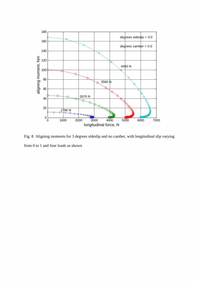
Fig. 8 Aligning moments for 3 degrees sideslip and no camber, with longitudinal slip varying

from 0 to 1 and four loads as shown

0 1000 2000 3000 4000 5000 6000 70000

1000

2000

3000

4000

5000

6000

7000

longitudinal force, N

side

forc

e, N

degrees sideslip = 6.0degrees camber = 0.0

1780 N

2670 N

3560 N

4450 N

Fig. 9 Shear forces for 6 degrees sideslip and no camber, with longitudinal slip varying from

zero to 1 and four loads as shown

0 1000 2000 3000 4000 5000 6000 7000-20

0

20

40

60

80

100

120

longitudinal force, N

alig

ning

mom

ent,

Nm

degrees sideslip = 6.0

degrees camber = 0.0

1780 N

2670 N

3560 N

4450 N

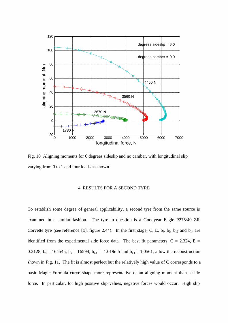
Fig. 10 Aligning moments for 6 degrees sideslip and no camber, with longitudinal slip

varying from 0 to 1 and four loads as shown

4 RESULTS FOR A SECOND TYRE

To establish some degree of general applicability, a second tyre from the same source is

examined in a similar fashion. The tyre in question is a Goodyear Eagle P275/40 ZR

Corvette tyre (see reference [1], figure 2.44). In the first stage, C, E, b4, b5, b13 and b14 are

identified from the experimental side force data. The best fit parameters, C = 2.324, E =

0.2128, b4 = 164545, b5 = 16594, b13 = -1.019e-5 and b14 = 1.0561, allow the reconstruction

shown in Fig. 11. The fit is almost perfect but the relatively high value of C corresponds to a

basic Magic Formula curve shape more representative of an aligning moment than a side

force. In particular, for high positive slip values, negative forces would occur. High slip

force values would be unreasonable with such a representation. Therefore, the value of C is

constrained to 1.65 and a new optimization of the remaining parameters carried out. This

gives almost as good a fit as the original, shown in Fig. 12. Clearly, with forces measured

only up to the peak, C and E can be traded off against each other, without the fit quality

altering much. C can be fixed, if desired, to control the high slip force behaviour of the tyre.

0 0.02 0.04 0.06 0.08 0.1 0.120

1000

2000

3000

4000

5000

6000

7000

8000

9000

slip angle, rad

late

ral f

orce

, N

1802 N

4094 N

6452 N

8704 N

Fig. 11 Reconstructed side forces for best fit C, E, b4, b5, b13 and b14. Solid lines show the

experimental results from reference [1]; Dotted lines show the fitted results

0 0.02 0.04 0.06 0.08 0.1 0.120

1000

2000

3000

4000

5000

6000

7000

8000

9000

slip angle, rad

late

ral f

orce

, N

1802 N

4094 N

6452 N

8704 N

Fig. 12 Side forces for best fit E, b4, b5, b13 and b14 (see below for coefficients) with C

constrained to be 1.65. Dotted lines show the fitted results

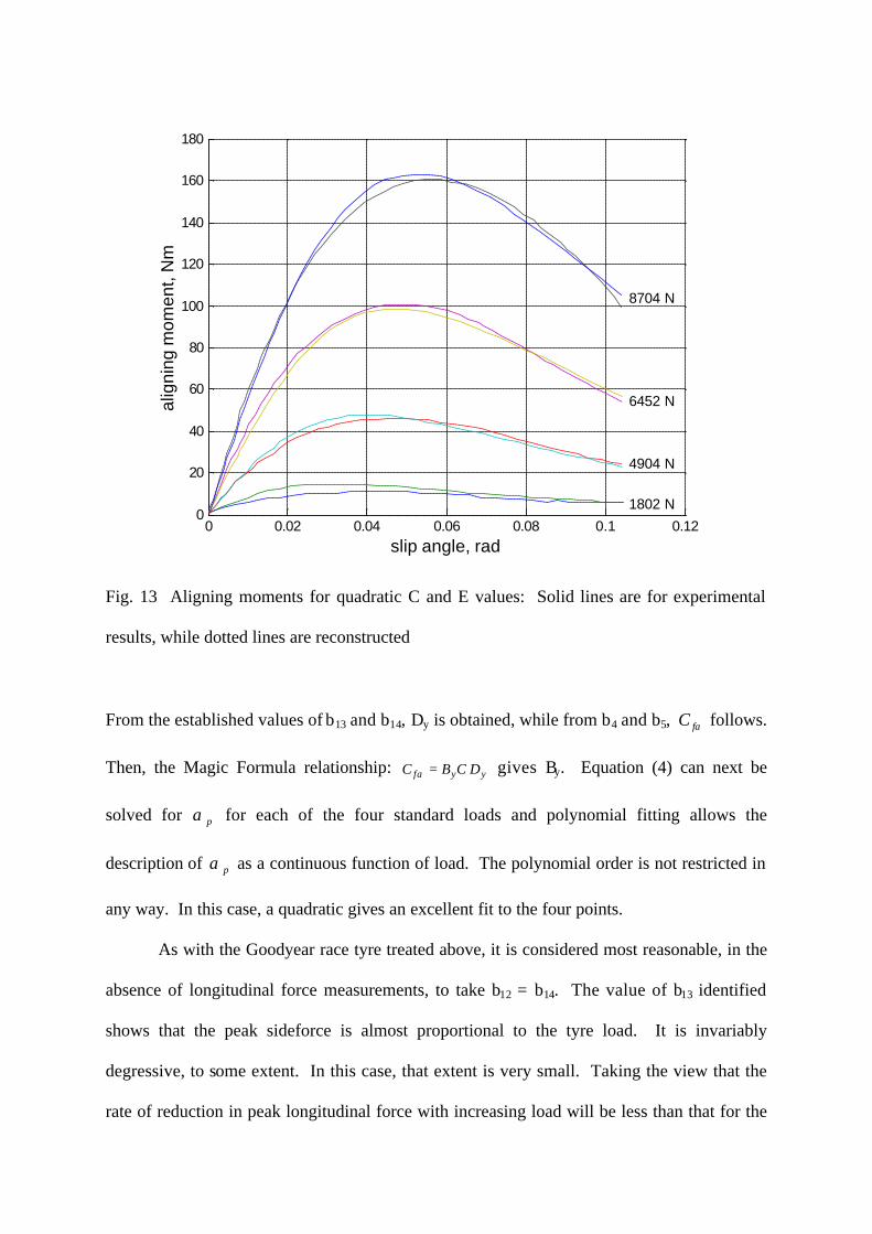
The aligning moment data allows the identification of the quadratic polynomial coefficients

of expressions for Cm and Em and the parameters b6, b7, b8, b15 and b16, with the results shown

in Fig. 13. As with the Goodyear race tyre, the quadratic variation of Cm and Em with load is

necessary to get a good fit.

0 0.02 0.04 0.06 0.08 0.1 0.120

20

40

60

80

100

120

140

160

180

slip angle, rad

alig

ning

mom

ent,

Nm

1802 N

4904 N

6452 N

8704 N

Fig. 13 Aligning moments for quadratic C and E values: Solid lines are for experimental

results, while dotted lines are reconstructed

From the established values of b13 and b14, Dy is obtained, while from b4 and b5, αfC follows.

Then, the Magic Formula relationship: yyf DCBC =α gives By. Equation (4) can next be

solved for pα for each of the four standard loads and polynomial fitting allows the

description of pα as a continuous function of load. The polynomial order is not restricted in

any way. In this case, a quadratic gives an excellent fit to the four points.

As with the Goodyear race tyre treated above, it is considered most reasonable, in the

absence of longitudinal force measurements, to take b12 = b14. The value of b13 identified

shows that the peak sideforce is almost proportional to the tyre load. It is invariably

degressive, to some extent. In this case, that extent is very small. Taking the view that the

rate of reduction in peak longitudinal force with increasing load will be less than that for the

lateral force, little scope is left for varying b11. It must be negative to get the normal

degressive behaviour, while it must be numerically small to compare properly with the lateral

properties. An estimate of b11 giving 4.2% more peak longitudinal force than peak lateral

force at the highest load of 8702 N is made on this basis. Further, a reasonable estimate of

the slip ratio for maximum longitudinal force, bearing in mind the rather strong dependence

of pα on load for this tyre, is that pκ will be proportional to load according to

zp Fe .64282.11176.0 −+=κ .

Putting the relevant values of C, E and pκ into equation (4) allows solving for Bx,

giving xxf DCBasC ..κ and the optimal coefficients b1, b2 and b3 relating Cfκ to load can then be

found via “fminsearch”. Camber influences are dealt with as for the Goodyear race tyre, with

a similar outcome, that g1 = 0.75, b9 = 5e-5 and b10 = 0.5. Slip_m follows from solution of

(4), with C, E and B=1/C given for the normalized Magic Formula.

Now the data set is complete as follows:

C = 1.65; B = 1/C; E = -0.44939; slip_m = 2.0563; g1 = 0.75;

Cm = Cmz1+Cmz2*Fz+Cmz3*Fz2 with Cmz1 = 2.2299; Cmz2 = 7.9288e-5; Cmz3 = 8.8059e-10;

Em = Emz1+Emz2*Fz+Emz3*Fz2 with Emz1 = 0.2852; Emz2 = 1.4025e-5; Emz3 = -1.9189e-10;

b1 = 1.8532e-9; b2 = 18.4831; b3 = 1.5889e-5;

b4 = 163179; b5 = 16433;

b6 = -2.1678e-8; b7 = 0.4772; b8 = -3.4432e-5;

b9 = 0.00005; b10 = 0.5;

b11 = -4.7248e-6; b12 = 1.0588;

b13 = -9.4496e-6; b14 = 1.0588;

b15 = 1.5556e-6; b16 = 5.205e-3;

κp = 1.4282e-6.Fz+0.11757; αp = 3.4735e-10.Fz2-7.03465e-7.Fz+0.10927.

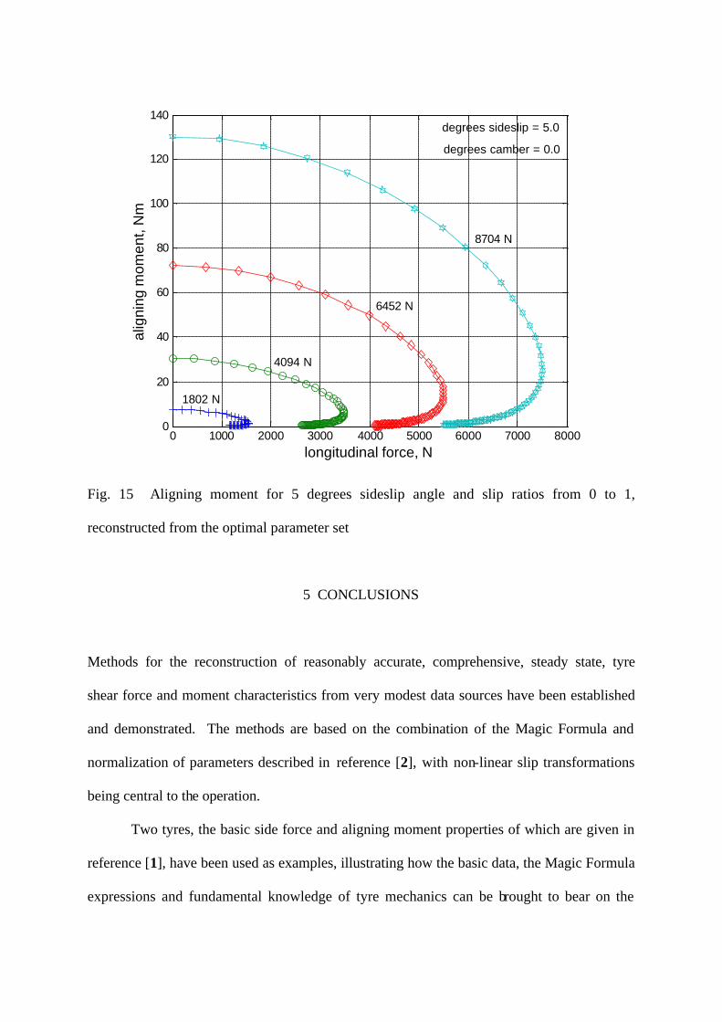
Combined slip forces and aligning moments derivable from this parameter set are

illustrated in Figs 14 and 15 for an arbitrary sideslip angle of 5 degrees (0.0873 rad).

Agreement of the results with the original measurements can be seen to be very good for both

side forces and aligning moments, by comparison of these results with those of Figs 12 and

13 for pure sideslip. The continuity of the forces and moments as the slip ratio increases is

also in evidence and the very high slip behaviour can be seen to be utterly reasonable in a

qualitative sense.

0 1000 2000 3000 4000 5000 6000 7000 80000

1000

2000

3000

4000

5000

6000

7000

8000

longitudinal force, N

side

forc

e, N

degrees sideslip = 5.0

degrees camber = 0.0

1802 N

4094 N

6452 N

8704 N

Fig. 14 Sideforce and braking force for 5 degrees sideslip angle and slip ratios from 0 to 1,

reconstructed from the optimal parameter set

0 1000 2000 3000 4000 5000 6000 7000 80000

20

40

60

80

100

120

140

longitudinal force, N

alig

ning

mom

ent,

Nm

degrees sideslip = 5.0

degrees camber = 0.0

1802 N

4094 N

6452 N

8704 N

Fig. 15 Aligning moment for 5 degrees sideslip angle and slip ratios from 0 to 1,

reconstructed from the optimal parameter set

5 CONCLUSIONS

Methods for the reconstruction of reasonably accurate, comprehensive, steady state, tyre

shear force and moment characteristics from very modest data sources have been established

and demonstrated. The methods are based on the combination of the Magic Formula and

normalization of parameters described in reference [2], with non-linear slip transformations

being central to the operation.

Two tyres, the basic side force and aligning moment properties of which are given in

reference [1], have been used as examples, illustrating how the basic data, the Magic Formula

expressions and fundamental knowledge of tyre mechanics can be brought to bear on the

problem of deriving a good set of parameters. Standard optimization software is needed to

make the method practical. The parameter set is easily convertible to tyre forces and

moments through the algorithm given, which is a small development of that in reference [2].

The shear forces and moments for pure lateral slip are recoverable without significant

distortion, through the normalization and de-normalization processes. The shear forces

associated with longitudinal slip have had to be estimates and results based on these estimates

have been shown to be quantitatively reasonable and qualitatively excellent. The analyst has

some choice in accentuating the accuracy of one or other aspect of the tyre force system. In

the circumstances in which the data used is entirely lateral force and aligning moment results

and parameters are chosen to match those results closely, no loss of precision is implied by

using the combined slip model, if the longitudinal slip values are small.

Comprehensive and useful tyre steady state shear force data can now be derived from

very limited measurements.

References

1 Milliken, W. F. and Milliken, D. L. Race Car Vehicle Dynamics, 1996 (SAE,

Warrendale).

2 Sharp, R. S. and Bettella, M. Tyre shear force and moment descriptions by normalization

of parameters and the “Magic Formula”, Vehicle System Dynamics, in press.

3 Pacejka, H. B. and Bakker, E. The Magic Formula tyre model, Proc. 1st International Tyre

Colloquium (H. B. Pacejka ed.), Delft, 1991, 1-18 (Supplement to Veh. Syst. Dynamics, 21,

Swets and Zeitlinger, Lisse).

4 Radt, H. S. and Glemming, D. A. Normalisation of tire force and moment data, Tire Sci.

and Technol., TSTCA, 1993, 21(2), 91-119.

5 Pacejka, H. B. and Sharp, R. S. Shear force generation by pneumatic tyres in steady state

conditions: a review of modeling aspects, Veh. Syst. Dynamics, 1991, 20, 121-176.

6 Genta, G. Motor Vehicle Dynamics: modeling and simulation, 1997 (World Scientific

Publishing, Singapore).

7 Clark, S. K. Mechanics of Pneumatic Tires 2nd edition, 1981, NBIS Monograph 122

(Washington DC).

8 Bakker, E., Nyborg, L. and Pacejka, H. B. Tyre modelling for use in vehicle dynamics

studies, SAE 870421, 1987.

Appendix – MATLAB function for calculation of forces and moment

function [Fx,Fy,Mz] = norm_alg(fz,kappa,alpha,gamma);

% Tyre shear force / moment calculations via Magic Formula and similarity method

C_fkappa = fz*(b1*fz+b2)/exp(b3*fz);

C_falpha = b4*sin(2*atan(fz/b5));

C_malpha = fz*(b6*fz+b7)/exp(b8*fz);

C_fgamma = fz*(b9*fz+b10);

C_m = C_mz1+(C_mz2+C_mz3*fz)*fz;

D_fx = fz*(b11*fz+b12);

D_fy = fz*(b13*fz+b14);

D_mz = fz*(b15*fz+b16);

E_m = E_mz1+(E_mz2+E_mz3*fz)*fz;

a_feq = alpha+gamma*(C_fgamma+g1*fz)/C_falpha;

if alpha == 0

alpha = eps;

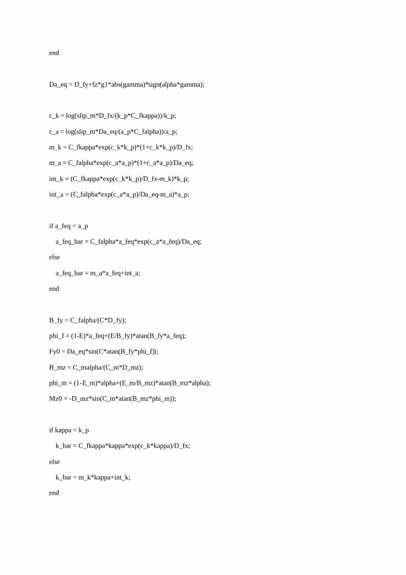
end

Da_eq = D_fy+fz*g1*abs(gamma)*sign(alpha*gamma);

c_k = log(slip_m*D_fx/(k_p*C_fkappa))/k_p;

c_a = log(slip_m*Da_eq/(a_p*C_falpha))/a_p;

m_k = C_fkappa*exp(c_k*k_p)*(1+c_k*k_p)/D_fx;

m_a = C_falpha*exp(c_a*a_p)*(1+c_a*a_p)/Da_eq;

int_k = (C_fkappa*exp(c_k*k_p)/D_fx-m_k)*k_p;

int_a = (C_falpha*exp(c_a*a_p)/Da_eq-m_a)*a_p;

if a_feq < a_p

a_feq_bar = C_falpha*a_feq*exp(c_a*a_feq)/Da_eq;

else

a_feq_bar = m_a*a_feq+int_a;

end

B_fy = C_falpha/(C*D_fy);

phi_f = (1-E)*a_feq+(E/B_fy)*atan(B_fy*a_feq);

Fy0 = Da_eq*sin(C*atan(B_fy*phi_f));

B_mz = C_malpha/(C_m*D_mz);

phi_m = (1-E_m)*alpha+(E_m/B_mz)*atan(B_mz*alpha);

Mz0 = -D_mz*sin(C_m*atan(B_mz*phi_m));

if kappa < k_p

k_bar = C_fkappa*kappa*exp(c_k*kappa)/D_fx;

else

k_bar = m_k*kappa+int_k;

end

l_bar = sqrt(a_feq_bar^2+k_bar^2);

phi_bar = (1-E)*l_bar+(E/B)*atan(B*l_bar);

Fs = sin(C*atan(B*phi_bar));

Fx = D_fx*Fs*k_bar/l_bar;

Fy = Da_eq*Fs*a_feq_bar/l_bar;

if Fy0 == 0

Fy0 = eps;

end

Mz = Mz0*(Fy/(Fy0))^2;

%*** *** ***