Tutorial 8: Frontal crash of a simplified truck model

TTuuttoorriiaall 88

FFrroonnttaall CCrraasshh

ooff aa SSiimmpplliiffiieedd

TTrruucckk MMooddeell

PPrroobblleemm ddeessccrriippttiioonn Outline Frontal crash of a simplified truck model against a rigid wall is

performed. Many of the basic elements needed to perform a full vehicle crash simulation are presented and typical results from such a simulation investigated.

Analysis type(s): Explicit

Element type(s): 3D Shell elements, Rigid Bodies, Beams and Bars

Materials law(s): Elasto-plastic

Model options: Boundary conditions, Spotwelds, Contact

Key results: Stress distributions and Impact forces

Prepared by: Date: Version:

Anthony Pickett, ESI GmbH/Institute for Aircraft Design, Stuttgart January 2008 V4 (Updated May 2012 for Visual-Crash PAM V8.0)

Tutorial 8: Frontal crash of a simplified truck model

Background information

Pre-processor, Solver and Post-processor used:

• Visual Crash PAM: To examine the truck model.

• Analysis (PAM-CRASH Explicit): To perform the explicit Finite Element analysis.

• Visual Viewer: Evaluating the results for contour plots, deformations and time history

information.

Prior knowledge for the exercise

This exercise is not worked through in detail and it is assumed that the reader has gained a good

working knowledge of using VCP from tutorials 1 through 7. The completed model of the simplified truck is provided and is examined using VCP.

Note the model is for teaching purposes and is a very simplified representation of a crash model using

circa 10,000 elements; todays models can typically use several millions of elements and are highly complex.

Problem data and description

Units: kN, mm, kg, ms

Description: The simplified truck model has

approximately 10,000 nodes and elements

in 48 material groups.

Loading: Impact mass of the truck is 1300kg which

impacts the rigid wall at 13,88m/sec.

Material: The materials used are mainly elasto-plastic

mild steel.

Supplied datasets

The completed truck model, including all entities, loadings, contacts and material/part properties is

provided and has the name:

Truck_Front.pc

CCoonntteennttss

Tutorial 8 ............................................................................................................. 1

Frontal Crash of a Simplified Truck Model .............................................................. 1

Problem description .............................................................................................. 1

Background information ........................................................................................ 2

Part 1: Using Visual Crash PAM to examine the simplified truck model .................... 3

Part 2: Examining and visualising some analysis results ......................................... 5

Tutorial 8: Frontal crash of a simplified truck model

Part 1: Using Visual Crash PAM to examine the simplified truck model

Starting Visual-Crash PAM and examining

the model

Start Visual Crash PAM and open the truck

model using Open File, then select the file:

Truck_Front.pc

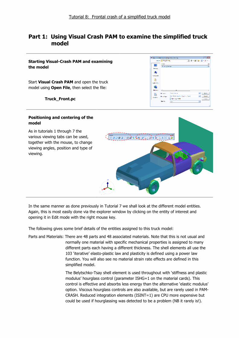
Positioning and centering of the

model

As in tutorials 1 through 7 the

various viewing tabs can be used,

together with the mouse, to change

viewing angles, position and type of

viewing.

In the same manner as done previously in Tutorial 7 we shall look at the different model entities.

Again, this is most easily done via the explorer window by clicking on the entity of interest and

opening it in Edit mode with the right mouse key.

The following gives some brief details of the entities assigned to this truck model:

Parts and Materials: There are 48 parts and 48 associated materials. Note that this is not usual and

normally one material with specific mechanical properties is assigned to many

different parts each having a different thickness. The shell elements all use the

103 ‘iterative’ elasto-plastic law and plasticity is defined using a power law

function. You will also see no material strain rate effects are defined in this

simplified model.

The Belytschko-Tsay shell element is used throughout with ‘stiffness and plastic

modulus’ hourglass control (parameter ISHG=1 on the material cards). This

control is effective and absorbs less energy than the alternative ‘elastic modulus’

option. Viscous hourglass controls are also available, but are rarely used in PAM-

CRASH. Reduced integration elements (ISINT=1) are CPU more expensive but

could be used if hourglassing was detected to be a problem (NB it rarely is!).

Tutorial 8: Frontal crash of a simplified truck model

Initial Velocities: Two initial velocity groups are defined for the car and the wall. The wall is

modelled using a single shell element and its velocities are set to zero by this

option. This shell element is used here for visualisation purposes and as a contact

surface in the segmented rigid wall definition (see later). All nodes in the truck

are given an initial impact velocity of 13.89m/sec.

Pressure faces: Constant internal pressure is applied to the inner surfaces of the tires. This is

reasonably accurate for tyre pressure, but the modern approach is to use an

airbag definition so pressure increases with tyre volume change during impact.

Contacts: The entire truck is placed in one single self contact definition (Type 36). Today,

this is computationally efficient and reliable; but care must be taken to make sure

there is no internal energy increase due to initial penetration of the elements.

This is especially necessary in coarse or approximately meshed models like this

training model. Notice in this model the contact thickness is only 0.5mm in order

to prevent (minimise) shell element initial penetration problems.

A type 34 contact is used to define contact between the vehicle (slave nodes)

and the wall (master elements). The wall is a fully fixed single shell element.

Rigid wall: A rigid wall could be used to define contact between the car and the wall impact

surface. However, this kinematic constraint can cause problems with other

kinematic constraints such as rigid bodies. Recent versions of PAM-CRASH do

data checks to avoid possible conflicts. The wall contact is therefore modelled as

a Type 34 penalty contact.

Rigid bodies: In total of 40 conventional rigid bodies have been defined to provide simple rigid

connection between different parts of the model.

Tied contacts: Two tied contacts have been used to connect coarse to fine meshes and avoid

the need for local remeshing. This can be a useful option, but it should not be

used in areas where important load transfer, or deformation mechanisms, may

occur.

Outputs: In total 11 nodal time history outputs and 6 sections have been defined. These

give time history information of individual nodes and force transfer through

sections of the structure. The information is saved on the .ERF file.

Pam Controls: The usual controls have been specified; however, in order to reduce CPU time

some timestep control options have been imposed (see control option TCTRL).

These timestep controls add some mass and/or modify local element mechanical

properties to meet the user specified minimum timestep limits. These options

must be used with care and some experience is needed.

Tutorial 8: Frontal crash of a simplified truck model

Part 2: Examining and visualising some analysis results The dataset is run with PAM-CRASH and the results are post-processed with Visual Viewer.

For results start Visual Viewer and open the results file, Truck_Front_RESULT.erfh5.

If information on the model units system is requested select MM, K, MS; this is important for plots and

especially if any numerical filters are to be used.

Global energy plots and numerical stability

First, the solution stability should

be checked by examining the

system energy balance. For this

study there is no energy input to

the system during the crash (from

external loads or imposed velocity/

displacements) and therefore the

total energy should be constant.

Plot the three global energy time

histories (Internal, External and

Total) using the options

highlighted. The total energy is

constant indicating a stable

solution.

Deformations

Next it is best to check deformations and contacts to see if results are sensible. The Truck_Front_

RESULT.erfh5 file also contains deformation and contour plots (e.g. plastic strain) at regular states

during the crash. Some example results are shown below.

Tutorial 8: Frontal crash of a simplified truck model

Other time histories

Material energies

A variety of other time history

information is available. The

adjacent plot shows typical

internal energy time history plots

(Entity Type > PART > Mat.

Internal energy) for three

selected materials.

Wall impact force

The wall impact force time

history is obtained from the

appropriate contact force time

history (wall contact).

Section force time histories

The adjacent view shows section

force time histories for three

sections (Entity Type >

SECTION). These are especially

useful to understand the load

transfer mechanisms in the

structure.

Tutorial 8: Frontal crash of a simplified truck model

Nodal time histories

Finally, time history information at nodes is shown with (Entity Type > NODE) and selection of the

required node and component. The displacement and velocity time histories generally have a smooth

shape; the acceleration signal,

however, has a very high

frequency that needs to be

filtered to get a meaningful

curve. The adjacent plot shows

the unfiltered (Acceleration

Magnitude - Component) for one

node, together with the filtered

version of the same data (in

green).

Remark: It is important to activate the Pre-Filter flag in the Pam Controls when using filters in

the post-processing. Also, the correct filter should be selected when comparing results to

filtered test results.

An unstable analysis

As a useful exercise it is suggested to change the

value of hcont in the self contact for this model

from 0.5 to 2.0 mm, export the new dataset

(Truck_Front_Hcont2.pc) and rerun the

analysis.

Investigating the .THP file in Visual Viewer it is

seen that there are sudden jumps in energies at

the start of the simulation. Plotting internal

energies for individual materials can help to

identify the location of this increase; alternatively,

looking at contour plots of plastic strain is another

possibility.

The instabilities are due to local element penetrations in the contact interface, causing temporary high

contact forces and materials plastification. Either the mesh should be ‘cleaned’, or options available in

VCP used to remove the initial penetrations (e.g. Checks > Penetration/ Intersection). The use

of a small hcont value can be effective, but is not really the best solution.