tutorial 6: manual srm data analysis - dia/swath...

SRM Course 2013 Tutorial 6 – Manual SRM data analysis

1

Tutorial 6: Manual SRM data analysis After the generation of a transition list and its measurement by SRM, the next step is quality control and data analysis of your runs. Skyline offers very useful graphical views that allow a fast and straightforward peak intensity and retention time comparison over many SRM runs. Tip! If you plan a large SRM measurement including lots of samples, it is well worth to invest time upfront on defining the optimal transition list for your samples in some refinement runs. This helps to avoid repeated measurement of transitions which are of bad quality or not informative. Tip! Import each data file into Skyline directly after the measurement to monitor data quality, i.e. sensitivity and reproducibility, which allows taking immediate action in case instrument problems occur. Tip! Select a few positive control peptides from the background proteome, which are monitored in each run and allow controlling sample quality and instrument performance over months and years. Ideally, positive control peptides do not change in abundance over the samples, i.e. they should come from housekeeping proteins. This allows normalisation and thus accounting for variability in sample preparation etc. Further, it is useful if these peptides cover a wide abundance range (high, medium, and low abundant peptides). Label-free SRM data analysis For training purposes we will start with label-free data analysis to highlight advantages and disadvantages of each of the workflows, label-free and label-based. 1. Setting up Skyline document

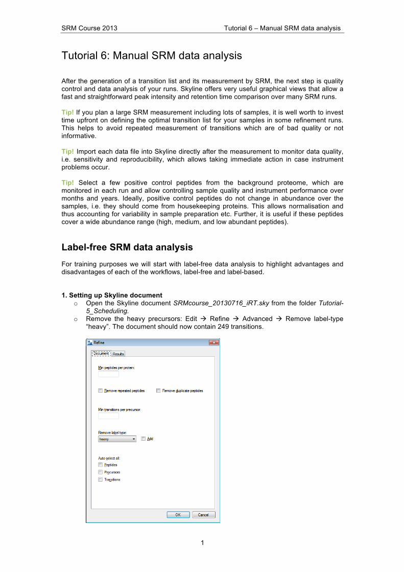
o Open the Skyline document SRMcourse_20130716_iRT.sky from the folder Tutorial-5_Scheduling.

o Remove the heavy precursors: Edit à Refine à Advanced à Remove label-type “heavy”. The document should now contain 249 transitions.


2

o Remove the calibration run: Edit à Manage results à Remove. o Save the Skyline file as SRMcourse_20130717_label-free.sky in the folder Tutorial-

6_ManualAnalysis.

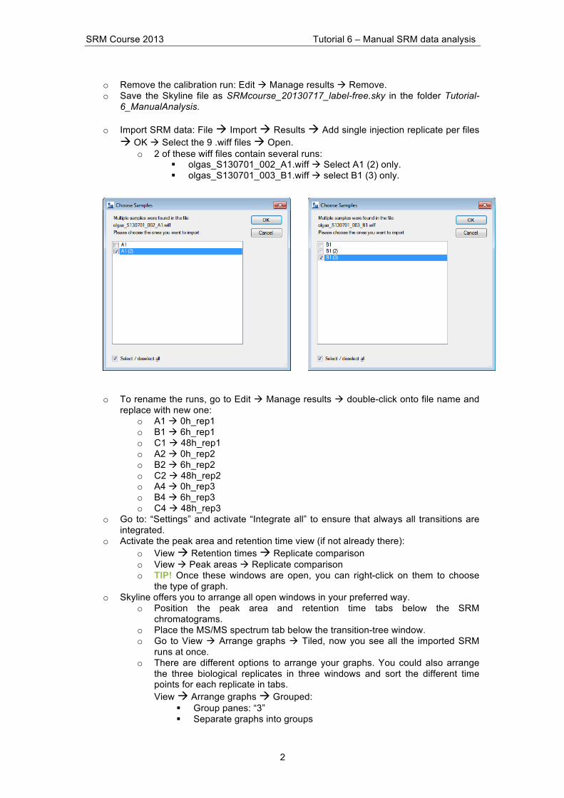
o Import SRM data: File à Import à Results à Add single injection replicate per files à OK à Select the 9 .wiff files à Open.

o 2 of these wiff files contain several runs: § olgas_S130701_002_A1.wiff à Select A1 (2) only. § olgas_S130701_003_B1.wiff à select B1 (3) only.

o To rename the runs, go to Edit à Manage results à double-click onto file name and replace with new one:

o A1 à 0h_rep1 o B1 à 6h_rep1 o C1 à 48h_rep1 o A2 à 0h_rep2 o B2 à 6h_rep2 o C2 à 48h_rep2 o A4 à 0h_rep3 o B4 à 6h_rep3 o C4 à 48h_rep3

o Go to: “Settings” and activate “Integrate all” to ensure that always all transitions are integrated.

o Activate the peak area and retention time view (if not already there): o View à Retention times à Replicate comparison o View à Peak areas à Replicate comparison o TIP! Once these windows are open, you can right-click on them to choose

the type of graph. o Skyline offers you to arrange all open windows in your preferred way.

o Position the peak area and retention time tabs below the SRM chromatograms.

o Place the MS/MS spectrum tab below the transition-tree window. o Go to View à Arrange graphs à Tiled, now you see all the imported SRM

runs at once. o There are different options to arrange your graphs. You could also arrange

the three biological replicates in three windows and sort the different time points for each replicate in tabs. View à Arrange graphs à Grouped:

§ Group panes: “3” § Separate graphs into groups


3

§ Sort order: “Document” § OK.

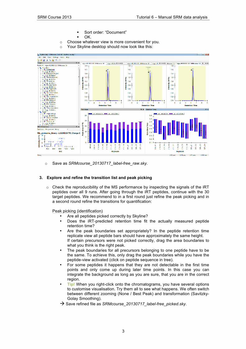
o Choose whatever view is more convenient for you. o Your Skyline desktop should now look like this:

o Save as SRMcourse_20130717_label-free_raw.sky. 3. Explore and refine the transition list and peak picking

o Check the reproducibility of the MS performance by inspecting the signals of the iRT

peptides over all 9 runs. After going through the iRT peptides, continue with the 30 target peptides. We recommend to in a first round just refine the peak picking and in a second round refine the transitions for quantification: Peak picking (identification)

• Are all peptides picked correctly by Skyline? • Does the iRT-predicted retention time fit the actually measured peptide

retention time? • Are the peak boundaries set appropriately? In the peptide retention time

replicate view all peptide bars should have approximately the same height. If certain precursors were not picked correctly, drag the area boundaries to what you think is the right peak.

• The peak boundaries for all precursors belonging to one peptide have to be the same. To achieve this, only drag the peak boundaries while you have the peptide-view activated (click on peptide sequence in tree).

• For some peptides it happens that they are not detectable in the first time points and only come up during later time points. In this case you can integrate the background as long as you are sure, that you are in the correct region.

• Tip! When you right-click onto the chromatograms, you have several options to customise visualisation. Try them all to see what happens. We often switch between different zooming (None / Best Peak) and transformation (Savitzky-Golay Smoothing).

à Save refined file as SRMcourse_20130717_label-free_picked.sky.


4

Transition refinement (quantification) • Are all transitions of good quality and reproducible over the samples? The

relative transition intensity has to be constant over all runs. To visualise this, right-click on the Peak Area tab and select “Normalized to total”.

• If certain transitions/precursors/peptides are of low quality (low intense, not co-eluting with the other transitions, shouldered, etc.) or irreproducible over runs, remove them from the document by deleting them from the transition tree window. Tip! You can bring back deleted transitions/precursors/peptides by right-clicking on the respective parent item à Pick children.

à Save the refined file as SRMcourse_20130717_label-free_refined.sky. 4. Export a custom-defined report

o Export all quantitative data to a .csv file for further processing.

• File à Export à Report • The Report tab offers you a range of predefined report formats. Here we will

generate our own report format: Edit list à Add. • An “Edit Report” window opens.

Note: For detailed information about all options see the Skyline tutorial “Skyline Custom Reports and Results Grids” on the Skyline website.

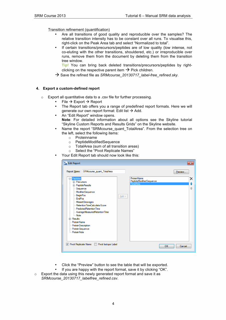
• Name the report “SRMcourse_quant_TotalArea”. From the selection tree on the left, select the following items:

o Proteinname o PeptideModifiedSequence o TotalArea (sum of all transition areas) o Select the “Pivot Replicate Names”

• Your Edit Report tab should now look like this:

• Click the “Preview” button to see the table that will be exported. • If you are happy with the report format, save it by clicking “OK”.

o Export the data using this newly generated report format and save it as SRMcourse_20130717_labelfree_refined.csv.


5

Label-based SRM data analysis So far we have identified and quantified our target peptides without using information of the isotope-labelled reference peptides that were spiked into the samples and measured along with the target peptides. Now we repeat the peak picking and transition refinement by including heavy modifications to your document. o Open the Skyline document SRMcourse_20130717_label-free_raw.sky. o Save it as SRMcourse_20130717_label.sky to the folder Tutorial-6_ManualAnalysis. o Add heavy peptides back into the document: Edit à Refine à Advanced à activate add

check box next to “Add” next to the “Remove label type” field à Select from drop-down menu “heavy””.

o To ensure proper import and matching of light and heavy precursors go to: Edit à Manage results à Reimport.

o Remove heavy iRT peptides: Edit à Refine à Remove missing results. The document should now contain 471 transitions.

o Save the Skyline file as SRMcourse_20130717_label_raw.sky. o Go through all peptides to pick the right peaks (à save as …_picked.sky) and refine the

transitions (à save as …_refined.sky) as described above, this time considering also the information from the heavy channel. Caution! Make sure that the integration boundaries of heavy and light peak groups are the same. To achieve this, only drag the peak boundaries while you have the peptide-view activated (click on peptide sequence in tree).

o Create a new report format called SRMcourse_quant_RatioToStandard by copying the previously generated one (SRMcourse_quant_TotalArea) and replacing “TotalArea” by “RatioToStandard”, which is the ratio of the sum of all transition areas.

o Save the exported report as SRMcourse_20130717_label_refined.csv. Exercises

1. What are advantages and disadvantages of label-free and label-based SRM data analysis?

2. How important is the careful placement of the peak boundaries in label-free compared to label-based data analysis?

3. Why should the ratio between a spike-in and an endogenous peptide ideally be

around 1 for accurate protein quantification?

4. Data analysis in Excel (only if time allows):

Statistics/Excel reminder

• Standard deviation: The standard deviation is a measure of how widely values are dispersed from the average value (the mean). à Standard deviation in Excel: STDEV.S(number1, number2, …)

• Coefficient of variance (CV): Normalise (divide) standard deviation by average and multiply by 100 to obtain the result in %.

Label-free SRM data analysis 1. Remove all iRT peptides and move the 48h columns to the end of the table. 2. Peptide level:


6

a. Calculate the TotalArea ratio of each of the 9 samples to the averaged TotalArea of time point 0h for each peptide.

b. Calculate the average, the standard deviation, and the CV of the TotalArea ratios over the 3 biological replicates per time point.

c. What is the average peptide-level CV over the whole dataset? 3. Protein level:

a. Average the TotalArea ratio of all precursors per protein for each of the 9 samples.

b. Calculate the average protein ratio, the standard deviation, and the CV over the three biological replicates.

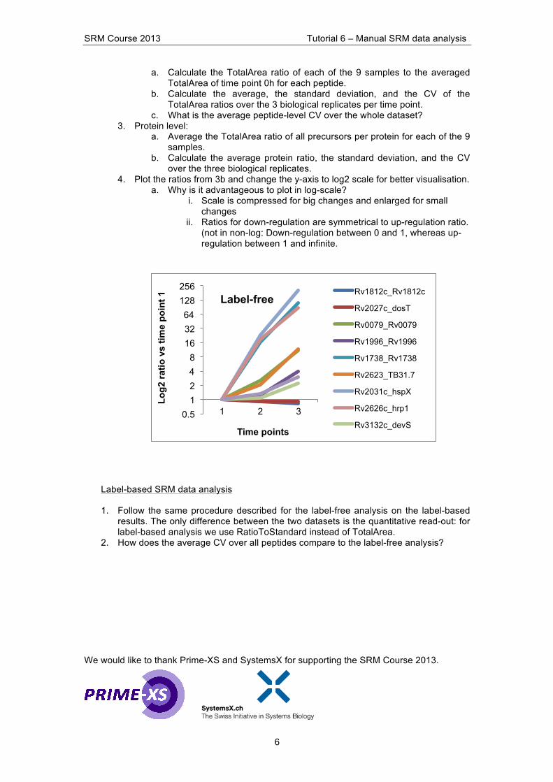
4. Plot the ratios from 3b and change the y-axis to log2 scale for better visualisation. a. Why is it advantageous to plot in log-scale?

i. Scale is compressed for big changes and enlarged for small changes

ii. Ratios for down-regulation are symmetrical to up-regulation ratio. (not in non-log: Down-regulation between 0 and 1, whereas up-regulation between 1 and infinite.

Label-based SRM data analysis

1. Follow the same procedure described for the label-free analysis on the label-based results. The only difference between the two datasets is the quantitative read-out: for label-based analysis we use RatioToStandard instead of TotalArea.

2. How does the average CV over all peptides compare to the label-free analysis? We would like to thank Prime-XS and SystemsX for supporting the SRM Course 2013.

0.5 1 2 4 8

16 32 64

128 256

1 2 3

Log2

ratio

vs

time

poin

t 1

Time points

Label-free Rv1812c_Rv1812c

Rv2027c_dosT

Rv0079_Rv0079

Rv1996_Rv1996

Rv1738_Rv1738

Rv2623_TB31.7

Rv2031c_hspX

Rv2626c_hrp1

Rv3132c_devS

tutorial 6: manual srm data analysis - dia/swath...

Documents