tutorial 2 materials and loading - siamfarm

Tutorial 2 Materials and Loading • Multiple material slope with weak layer • Pore pressure defined by water table • Uniformly distributed external load • Circular slip surface search (Grid search)

Slide v.7.0 Tutorial Manual Tutorial 2: Materials & Loading

Introduction This tutorial will demonstrate how to model a more complex multi-material slope, with both pore water pressure and an external load.

The finished product of this tutorial can be found in the Tutorial 02 Materials and Loading.slim data file. All tutorial files installed with Slide 7.0 can be accessed by selecting File > Recent Folders > Tutorials Folder from the Slide main menu.

Model If you have not already done so, run the Slide Model program by double-clicking on the Slide icon in your installation folder. Or from the Start menu, select Programs → Rocscience → Slide 7.0 → Slide.

If the Slide application window is not already maximized, maximize it now, so that the full screen is available for viewing the model.

Project Settings

Although we do not need to set any Project Settings for this tutorial, let’s briefly examine the Project Settings dialog.

Select: Analysis → Project Settings

Select the Groundwater page from the list at the left of the dialog.

Notice the various methods of defining pore pressure conditions in Slide. For this tutorial, we will be using the default (Groundwater Method = Water Surfaces). This allows pore pressure to be calculated from a Water Table or Piezometric surfaces.

We will be using all of the default selections in Project Settings. However, select the Project Summary page, and enter a Project Title – Materials & Loading Tutorial. Select OK.

2 - 2


Add External Boundary

The first boundary that must be defined for every Slide model is the External Boundary (see the Quick Start Tutorial for a definition of the External Boundary in Slide).

To add the External Boundary, select Add External Boundary from the toolbar or the Boundaries menu.

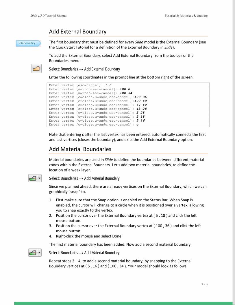
Select: Boundaries → Add External Boundary

Enter the following coordinates in the prompt line at the bottom right of the screen.

Enter vertex [esc=cancel]: 5 0 Enter vertex [u=undo,esc=cancel]: 100 0 Enter vertex [u=undo,esc=cancel]: 100 34 Enter vertex [c=close,u=undo,esc=cancel]:100 36 Enter vertex [c=close,u=undo,esc=cancel]:100 40 Enter vertex [c=close,u=undo,esc=cancel]: 67 40 Enter vertex [c=close,u=undo,esc=cancel]: 43 28 Enter vertex [c=close,u=undo,esc=cancel]: 5 28 Enter vertex [c=close,u=undo,esc=cancel]: 5 18 Enter vertex [c=close,u=undo,esc=cancel]: 5 16 Enter vertex [c=close,u=undo,esc=cancel]: c

Note that entering c after the last vertex has been entered, automatically connects the first and last vertices (closes the boundary), and exits the Add External Boundary option.

Add Material Boundaries

Material boundaries are used in Slide to define the boundaries between different material zones within the External Boundary. Let’s add two material boundaries, to define the location of a weak layer.

Select: Boundaries → Add Material Boundary

Since we planned ahead, there are already vertices on the External Boundary, which we can graphically “snap” to.

1. First make sure that the Snap option is enabled on the Status Bar. When Snap is enabled, the cursor will change to a circle when it is positioned over a vertex, allowing you to snap exactly to the vertex.

2. Position the cursor over the External Boundary vertex at ( 5 , 18 ) and click the left mouse button.

3. Position the cursor over the External Boundary vertex at ( 100 , 36 ) and click the left mouse button.

4. Right-click the mouse and select Done.

The first material boundary has been added. Now add a second material boundary.

Select: Boundaries → Add Material Boundary

Repeat steps 2 – 4, to add a second material boundary, by snapping to the External Boundary vertices at ( 5 , 16 ) and ( 100 , 34 ). Your model should look as follows:

2 - 3


Add Water Table

Now let’s add the water table, in order to define the pore pressure conditions.

Select: Boundaries → Add Water Table

You should still be in Snap mode, so use the mouse to snap the first two vertices to existing External Boundary vertices, and enter the rest of the vertices in the prompt line.

Enter vertex [esc=cancel]: use the mouse to snap to the vertex at 5 28 Enter vertex [u=undo,esc=cancel]: use the mouse to snap to the vertex at 43 28 Enter vertex [u=undo,esc=cancel]: 49 30 Enter vertex [c=close,u=undo,esc=cancel]: 60 34 Enter vertex [c=close,u=undo,esc=cancel]: 66 36 Enter vertex [c=close,u=undo,esc=cancel]: 74 38 Enter vertex [c=close,u=undo,esc=cancel]: 80 38.5 Enter vertex [c=close,u=undo,esc=cancel]: 100 38.5 Enter vertex [c=close,u=undo,esc=cancel]:press Enter or right-click and select Done

You will now see the Assign Water Table dialog.

2 - 4


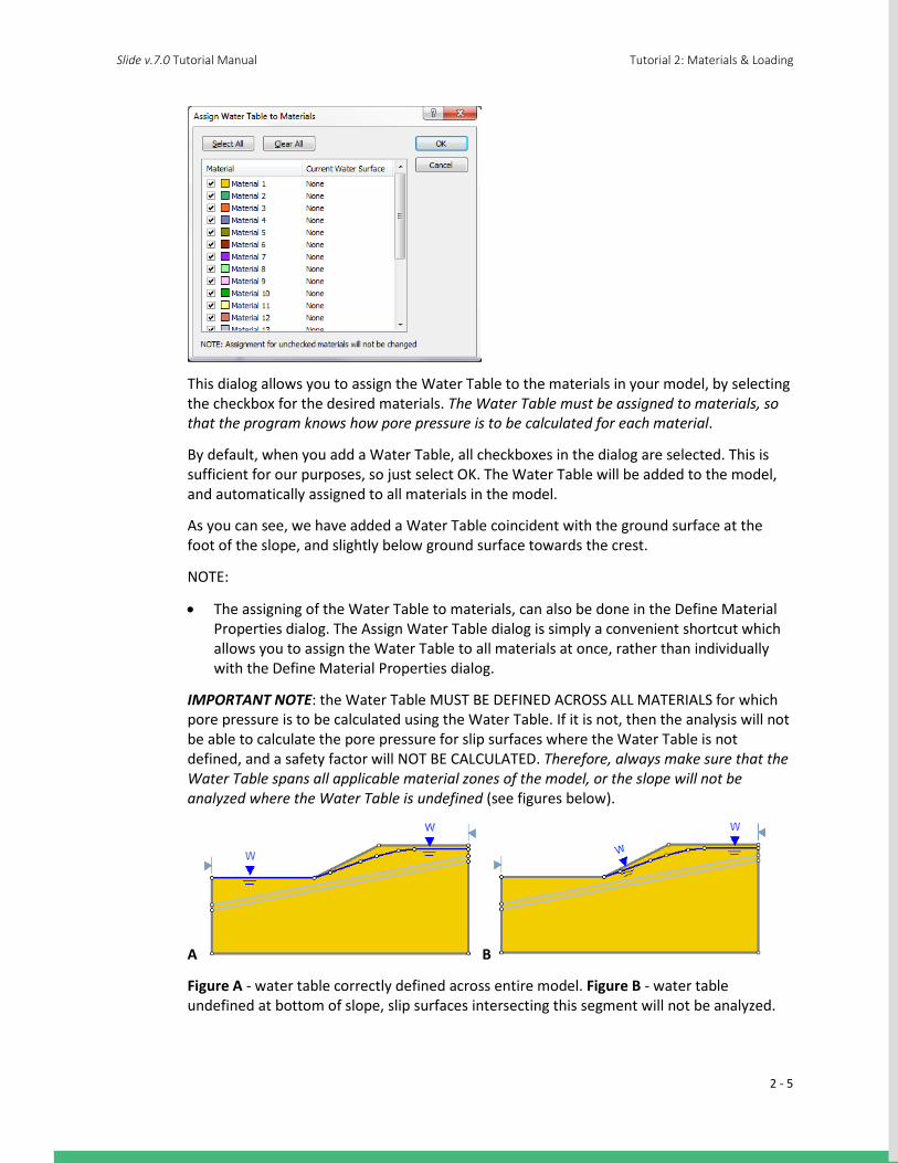
This dialog allows you to assign the Water Table to the materials in your model, by selecting the checkbox for the desired materials. The Water Table must be assigned to materials, so that the program knows how pore pressure is to be calculated for each material.

By default, when you add a Water Table, all checkboxes in the dialog are selected. This is sufficient for our purposes, so just select OK. The Water Table will be added to the model, and automatically assigned to all materials in the model.

As you can see, we have added a Water Table coincident with the ground surface at the foot of the slope, and slightly below ground surface towards the crest.

NOTE:

• The assigning of the Water Table to materials, can also be done in the Define Material Properties dialog. The Assign Water Table dialog is simply a convenient shortcut which allows you to assign the Water Table to all materials at once, rather than individually with the Define Material Properties dialog.

IMPORTANT NOTE: the Water Table MUST BE DEFINED ACROSS ALL MATERIALS for which pore pressure is to be calculated using the Water Table. If it is not, then the analysis will not be able to calculate the pore pressure for slip surfaces where the Water Table is not defined, and a safety factor will NOT BE CALCULATED. Therefore, always make sure that the Water Table spans all applicable material zones of the model, or the slope will not be analyzed where the Water Table is undefined (see figures below).

A B

Figure A - water table correctly defined across entire model. Figure B - water table undefined at bottom of slope, slip surfaces intersecting this segment will not be analyzed.

2 - 5


Add Distributed Load

In Slide, external loads can be defined as either concentrated line loads, or distributed loads. For this tutorial, we will add a uniformly distributed load near the crest of the slope.

Select the Loading & Support workflow tab, and select Add Distributed Load from the toolbar or the Loading menu.

Select: Loading → Add Distributed Load

You will see the Add Distributed Load dialog.

Enter a Magnitude = 50 kPa. Leave all other parameters at their default settings. Select OK.

Now as you move the cursor, you will see a small red cross which follows the cursor and snaps to the nearest point on the nearest boundary.

You may enter the location of the load graphically, by clicking the left mouse button when the red cross is at the desired starting and ending points of the distributed load. However, to enter exact coordinates, it is easier in this case to enter the coordinates in the prompt line.

Enter first point on boundary [esc=quit]: 70 40 Enter second point on boundary [esc=quit]: 80 40

The distributed load will be added to the model after you enter the second point. The distributed load is represented by red arrows pointing normal (downwards, in this case) to the External Boundary, between the two points you entered. The load magnitude is also displayed.

2 - 6


Slip Surfaces

For this tutorial, we will be performing a circular surface Grid Search, to attempt to locate the critical slip surface (i.e. the slip surface with the lowest safety factor).

A Grid Search requires a grid of slip centers to be defined. We will use the Auto Grid option, which automatically locates a grid for the user. Select the Surfaces workflow tab.

Select: Surfaces → Auto Grid

You will see the Grid Spacing dialog.

Enter an interval spacing of 20 x 20. Select OK.

The Grid will be added to the model, and your screen should appear as follows:

NOTE: slip center grids, and the circular surface Grid Search, are discussed in more detail in the Quick Start Tutorial. Please refer to that tutorial, or the Slide Help system, for more information.

2 - 7


Properties

It’s time to define our material properties. Select Define Materials from the toolbar or the Properties menu.

Select: Properties → Define Materials

With the first (default) material selected in the Define Materials dialog, enter the following properties:

• Name = Soil 1 • Unit Weight = 19 • Strength Type = Mohr-Coulomb • Cohesion = 28.5 • Phi = 20 • Water Surface = Water Table • Hu = 1

Enter the parameters shown above. Notice that the Water Surface = Water Table, because we already assigned the Water Table to all materials in the model, with the Assign Water Table dialog, when we created the Water Table. When all parameters are entered for the first material, select the second material, and enter the properties for the weak soil layer.

2 - 8


• Name = weak layer • Unit Weight = 18.5 • Strength Type = Mohr-Coulomb • Cohesion = 0 • Phi = 10 • Water Surface = Water Table • Hu = 1

Enter the properties, and select OK when finished.

Note the following about the Water Parameters:

• Water Surface = Water Table means that the Water Table will be used for pore pressure calculations for the material.

• In Slide, the Hu coefficient is defined as the factor by which the vertical distance to a water table (or piezo line) is multiplied to obtain the pressure head. It may range between 0 and 1. Hu = 1 would indicate hydrostatic conditions. Hu = 0 would indicate a dry soil, and intermediate values are used to simulate head loss due to seepage, as shown in the margin figure.

hp d

Hu = hp / d

2 - 9


Assigning Properties

Since we have defined two materials, it will be necessary to assign properties to the correct regions of the model, using the Assign Properties option.

Select Assign Properties from the toolbar or the Properties menu.

Select: Properties → Assign Properties

You will see the Assign Properties dialog, shown in the margin.

Before we proceed, note that:

• By default, when boundaries are created, Slide automatically assigns the properties of the first material in the Define Material Properties dialog, to all soil regions of the model.

• Therefore, in this case, we only need to assign properties to the weak layer of the model. The soil above and below the weak layer, already has the correct properties, of the first material which we defined.

To assign properties to the weak layer will only take two mouse clicks:

1. Use the mouse to select the “weak layer” soil, in the Assign Properties dialog (notice that the material names are the names you entered in the Define Material Properties dialog).

2. Now place the cursor anywhere in the “weak layer” of the model (i.e. anywhere in the narrow region between the two material boundaries), and click the left mouse button.

That’s it, properties are assigned. Notice that the weak layer zone now has the colour of the weak layer material. Close the Assign Properties dialog by selecting the X in the upper right corner of the dialog (or you can press the Escape key to close the dialog).

TIP: assigning can also be done using a right-click shortcut (right-click in the desired area and the popup menu will have an Assign Material submenu).

We are now finished creating the model, and can proceed to run the analysis and interpret the results.

2 - 10


Compute Before you analyze your model, save it as a file called tutorial02.slim. (Slide model files have a .slim filename extension).

Select: File → Save

Use the Save As dialog to save the file. You are now ready to run the analysis.

Select: Analysis → Compute

The Slide Compute engine will proceed in running the analysis. When completed, you are ready to view the results in Interpret.

2 - 11


Interpret To view the results of the analysis:

Select: Analysis → Interpret

This will start the Slide Interpret program. You should see the following figure.

As you can see, the Global Minimum slip circle, for the Bishop analysis method, passes through the weak layer, and is partially underneath the distributed load.

The weak layer and the external load clearly have an influence on the stability of this model, and the Global Minimum safety factor (Bishop analysis) is 0.797, indicating an unstable situation (safety factor < 1). This slope will require support, or other design modifications, if it is to be stabilized.

Using the drop-list in the toolbar, select other analysis methods, and view the Global Minimum surface for each. In this case, the actual surface, for the methods used (Bishop and Janbu) is the same, although different safety factors are calculated by each method.

In general, the Global Minimum surface will not necessarily be the same surface, for each analysis method. See the Quick Start Tutorial for further discussion about the Global Minimum surface.

Now select the Minimum Surfaces option from the toolbar or the Data menu, in order to view the minimum surface calculated at each grid point in the slip center grid.

Select: Data → Minimum Surfaces

The effect of the weak layer is even more dramatically visible. The minimum circles with the lowest safety factors are all tending to pass through the weak layer, as illustrated in the figure below.

2 - 12


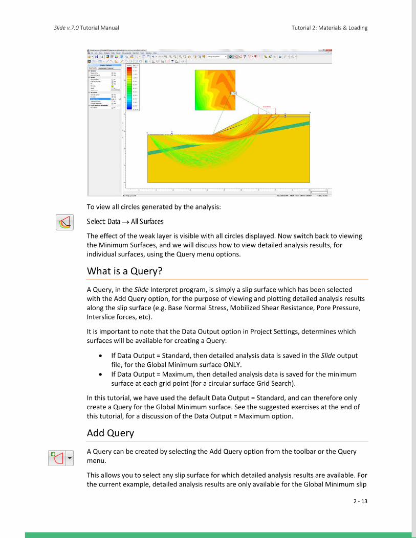
To view all circles generated by the analysis:

Select: Data → All Surfaces

The effect of the weak layer is visible with all circles displayed. Now switch back to viewing the Minimum Surfaces, and we will discuss how to view detailed analysis results, for individual surfaces, using the Query menu options.

What is a Query?

A Query, in the Slide Interpret program, is simply a slip surface which has been selected with the Add Query option, for the purpose of viewing and plotting detailed analysis results along the slip surface (e.g. Base Normal Stress, Mobilized Shear Resistance, Pore Pressure, Interslice forces, etc).

It is important to note that the Data Output option in Project Settings, determines which surfaces will be available for creating a Query:

• If Data Output = Standard, then detailed analysis data is saved in the Slide output file, for the Global Minimum surface ONLY.

• If Data Output = Maximum, then detailed analysis data is saved for the minimum surface at each grid point (for a circular surface Grid Search).

In this tutorial, we have used the default Data Output = Standard, and can therefore only create a Query for the Global Minimum surface. See the suggested exercises at the end of this tutorial, for a discussion of the Data Output = Maximum option.

Add Query

A Query can be created by selecting the Add Query option from the toolbar or the Query menu.

This allows you to select any slip surface for which detailed analysis results are available. For the current example, detailed analysis results are only available for the Global Minimum slip

2 - 13


surface, as discussed in the previous section.

When it is only required to create a Query for the Global Minimum, there are several time-saving shortcuts available. For example:

1. Right-click the mouse anywhere on the Global Minimum slip surface.

NOTE: you may click on the slip surface, or on the radial lines joining the slip center to the slip surface endpoints.

2. Select Add Query from the popup menu, and a Query will be created for the Global Minimum.

3. NOTE that the colour of the Global Minimum surface changes to black, to indicate that a query has been added. (Queries are displayed using black. The Global Minimum, before the query was added, was displayed in green. These colours can be customized in Display Options.)

You will find this a useful and frequently used shortcut for adding a Query for the Global Minimum.

Other shortcuts for adding and graphing Queries are described in the following sections.

Graph Query

The main reason for creating a Query, is to be able to graph detailed analysis results for the slip surface.

This is done with the Graph Query option in the toolbar or the Query menu.

Select: Query → Graph Query

NOTE:

• If only a single query exists, as in the current example, it will automatically be selected as soon as you select Graph Query, and you will immediately see the Graph Slice Data dialog, shown below. If more than one query exists, you will first have to select one (or more) queries, with the mouse.

1. In the Graph Slice Data dialog, select the data you would like to plot from the Primary data drop-list. For example, select Base Normal Stress.

2. Select the Horizontal axis data you would like to use (Distance, Slice number, or X coordinate).

2 - 14


3. Select Create Plot and Slide will create a plot as shown in the following figure.

More Query Shortcuts

Here are more useful shortcuts for adding / graphing Queries (these are left as optional exercises after completing this tutorial):

• If you right-click on the Global Minimum BEFORE a query is created, you can select Add Query, or Add Query and Graph from the popup menu. Or if you right-click AFTER a Query is created, you can select Graph Query or other options.

• Another very quick shortcut – if NO Queries have been created, and you select Graph Query from the toolbar, Slide will automatically create a Query for the Global Minimum, and display the Graph Slice Data dialog.

• Similarly, if you select Show Slices or Query Slice Data, a query will automatically be created for the Global Minimum, if it did not already exist.

2 - 15


Customizing a Graph

After a slice data graph has been created, many options are available to customize the graph data and appearance. These options are available through the sidebar, or the right-click menu.

Chart Properties

Right-click the mouse on a graph, and select Chart Properties. The Chart Properties dialog allows you to change axis titles, minimum and maximum values, etc. This is left as an optional exercise for the user to explore.

Change Plot Data

Right-click the mouse on a graph, and select Change Plot Data. This will display the Graph Slice Data dialog, allowing you to plot different data if you wish, while still remaining in the same view.

Changing the analysis method

After a graph is created, you can even change the analysis method. Simply select a method from the toolbar, and data corresponding to the method will be displayed.

NOTE:

• Depending on the data being viewed, results may or may not vary with analysis method. For example, Slice Weight will NOT vary with analysis method. Base Normal Stress will vary with analysis method.

• Also, “No Data” may be displayed, if the minimum surface for the analysis method chosen, is different from the surface on which you originally added the query.

Close this graph, so that we can demonstrate a few more features of the Slide query menu.

2 - 16


Show Slices

The Show Slices option is used to display the actual slices used in the analysis, on all existing queries in the current view.

Select: Query → Show Slices

The slices are now displayed for the Global Minimum.

Use the Zoom options to get a closer view, so that your screen looks similar to the following figure. Notice that there are 50 slices, which is the default number entered in Project Settings.

The Show Slices option can also be used for other display purposes, as configured in the Display Options in the sidebar or right-click menu. For example:

1. Right-click the mouse and select Display Options. Select the Slope Stability tab. 2. Turn OFF Slice Boundaries, and turn ON Hatch background. Observe the 45 degree

hatch pattern which now fills the failure mass. 3. Change the Fill colour, and select a different Hatch pattern. Experiment with

different combinations of Slice Display Options, and observe the results.

Remember that the Show Slices option only displays the Slice options that are turned ON in the Display Options dialog.

NOTE: the current Display Options can be saved as the program defaults, by selecting the Defaults button in the Display Options dialog, and then selecting “Make current settings the default” in the Defaults dialog.

2 - 17


Query Slice Data

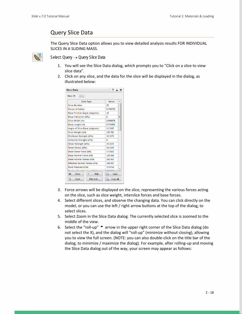
The Query Slice Data option allows you to view detailed analysis results FOR INDIVIDUAL SLICES IN A SLIDING MASS.

Select: Query → Query Slice Data

1. You will see the Slice Data dialog, which prompts you to “Click on a slice to view slice data”.

2. Click on any slice, and the data for the slice will be displayed in the dialog, as illustrated below:

3. Force arrows will be displayed on the slice, representing the various forces acting on the slice, such as slice weight, interslice forces and base forces.

4. Select different slices, and observe the changing data. You can click directly on the model, or you can use the left / right arrow buttons at the top of the dialog, to select slices.

5. Select Zoom in the Slice Data dialog. The currently selected slice is zoomed to the middle of the view.

6. Select the “roll-up” arrow in the upper right corner of the Slice Data dialog (do not select the X), and the dialog will “roll-up” (minimize without closing), allowing you to view the full screen. (NOTE: you can also double-click on the title bar of the dialog, to minimize / maximize the dialog). For example, after rolling-up and moving the Slice Data dialog out of the way, your screen may appear as follows:

2 - 18


7. Maximize the Slice Data dialog, by selecting the “roll-down” arrow, or double-clicking on the title bar of the dialog. Select the Hide / Show buttons, and view the results.

8. The Copy button will copy the current slice data to the Windows clipboard, where it can be pasted into another Windows application (e.g. for report writing).

9. The Filter List button allows you to customize the list of data which appears in the dialog.

10. Close the Slice Data dialog by selecting the X in the upper right-corner of the dialog, or press Escape.

11. Press F2 to Zoom All.

2 - 19


Deleting Queries

Queries can be deleted with the Delete Query option in the toolbar or the Query menu.

A convenient short-cut for deleting an individual query, is to right-click on a query, and select Delete Query. For example:

1. Right-click on the Global Minimum query. (You can right-click anywhere on the slip surface, or on the radial lines joining the slip center to the slip surface endpoints).

2. Select Delete Query from the popup menu, and the query will be deleted. (The Global Minimum is now displayed in green once again, indicating that the query no longer exists).

Show Values Along Surface

Another very useful option for viewing slip surface data is the Show Values Along Surface option. This allows you to visually plot data directly along the Global Minimum slip surface, or any slip surface for which a Query has been created.

Select: Query → Show Values Along Surface

You will see the following dialog.

1. Choose the Slice Data to plot, for example Base Normal Stress.

2. You will see the data plotted along the Global Minimum slip surface as shown in the following figure. The size of the bars represents the relative magnitude of the data on the base of each slice.

2 - 20


3. Choose different Slice Data types and observe the results. 4. Experiment with the various display options in the dialog and observe the results. 5. Choose Slice Data = None and close the dialog.

NOTE: the Show Values Along Surface option is also available as a right-click shortcut. If you right-click on the Global Minimum slip surface, or any other slip surface for which a Query has been created, the Show Values Along Surface option will be available in the popup menu. From the sub-menu you can directly choose a data type to plot, or access the Show Values dialog.

2 - 21


Graph SF along Slope

We will demonstrate one more data interpretation feature of Slide.

Select: Data → Graph SF along Slope

In the following dialog, select Create Plot:

This will create a plot of the factor of safety along the surface of the slope. The factor of safety values are obtained from each slip surface / slope intersection point.

This graph is useful in determing areas of the slope which correspond to slip surfaces with low safety factors, and may possibly be involved in failure. You may find it useful to tile the views horizontally, to view the graph and the slope together.

Select: Window → Tile Horizontally

Use the Zoom options as necessary, to achieve the desired view of the slope, relative to the graph. (Tip: first select Zoom All. Then use Zoom Mouse, and Pan, if necessary, to zoom the slope to the same scale as the graph).

2 - 22


Additional Exercises A safety factor graph, such as the previous figure, can be used to help refine a critical surface search, with the Define Slope Limits option, as suggested in the optional exercise below.

1. Return to the Slide Model program. 2. Use the Define Slope Limits dialog (see the Quick Start tutorial), to define two sets

of Slope Limits, corresponding approximately to the low safety factor areas of the safety factor graph shown in the previous figure.

3. Re-run the analysis, and see if a lower safety factor Global Minimum surface has been located.

Other Search Methods

The Grid Search is not the only search method available in Slide for circular slip surfaces. Other methods can be used. Re-run the analysis using:

• Slope Search method • Auto Refine Search method

and compare results. Experiment with different search method parameters. See the Slide Help system for information about the search methods.

Maximum Data Output Option

While demonstrating the Query options in this tutorial, we have pointed out that a Query could only be created for the Global Minimum surface. This is because we used the Data Output = Standard option in the Project Settings dialog.

If we use the Data Output = Maximum option, then a Query can be created for the minimum safety factor surface at any grid point, since detailed analysis data is then saved for all of these surfaces, and not just for the Global Minimum.

The following suggested exercise will demonstrate the capabilities of Slide when Data Output = Maximum.

1. Return to the Slide Model program, and set Data Output = Maximum in Project Settings.

2. Re-run the analysis. 3. In Slide Interpret, select Add Query from the toolbar or the menu. 4. Now hover the mouse (without clicking) over the slip center grid, or over the slip

surfaces within the slope. As you move the mouse, notice that the nearest corresponding slip surface is highlighted. (Note: it is helpful to turn on the Minimum Surfaces option first, since these are all of the surfaces for which you can create a Query).

5. When a desired slip surface has been located, click the left mouse button, and a Query will be created for that surface.

6. You may repeat steps 3-5, to add any number of Queries for different slip surfaces.

2 - 23


7. When using the Graph Query option (selected from the toolbar or the menu), you may graph multiple Queries on the same plot, by simply selecting the desired queries with the mouse.

NOTE: when Data Output = Maximum, the apparent compute speed may be significantly slower than when Data Output = Standard. Also, the size of the output files will be much larger, due to the large amount of data being stored. Depending on the number of slip surfaces you are analyzing, these differences can be very significant. Data Output = Maximum option should only be used when you wish to view detailed data for surfaces other than the Global Minimum.

That concludes this tutorial. To exit the program:

Select: File → Exit

2 - 24

tutorial 2 materials and loading - siamfarm

Documents