a first tutorial in stata - ncer · a first tutorial in stata ... loading an excel file stan hurn...

A First Tutorial in Stata

Stan Hurn

Queensland University of TechnologyNational Centre for Econometric Research

www.ncer.edu.au

Stan Hurn (NCER) Stata Tutorial 1 / 66

www.ncer.edu.au

Table of contents

1 Preliminaries

2 Loading Data

3 Basic Descriptive Statistics

4 Basic Plotting

5 Simple Data Manipulation

6 Simple Linear Regression

7 Using do files

8 Some Regression ExamplesElectricity DataCalifornia Schools DataFood Expenditure and Income

9 Instrumental Variables EstimationWage DataArtificial Data


Preliminaries

Stata

Stata is a fast, powerful statistical package with

smart data-management facilities,

a wide array of up-to-date statistical techniques,

and an excellent system for producing publication-quality graphs

The bad news is that Stata is NOT as easy to use as some other statisticalpackages, but Version 12 has got a reasonable menu-driven interface. On thewhole the advantages probably outweigh the steepness of the initial learning curve.


Preliminaries

Stata Resources

One of the major advantages to using Stata is that there are a large number ofhelpful resources to be found. For example:

a good web-based tutorial can be found athttp://data.princeton.edu/stata/default.html

a useful introductory book isAn Introduction to Modern Econometrics Using Stata by Christopher F. Baumpublished by Stata Press in 2006


http://data.princeton.edu/stata/default.html

Preliminaries

The Stata 12 Front End for Mac


Preliminaries

The Stata 12 Front End for Windows


Preliminaries

Stata 12 Front End

Stata has an menu bar on the top and 5 internal windows.

The main window is the one in the middle (1 on the previous slide). It givesyou the all output of you operations in Stata.

The Command window (2) executes commands. You can type commandsdirectly in this window as an alternative to using the menu system.

The Review window (3), lists all the operations preformed since openingStata. If you click on one of your past commands, you will see the commandbeing displayed in the Command window and you can re-run it by hitting theenter key.

The Variables window (4) lists the variables in the current dataset (and theirdescriptions). When you double-click on the variable, it appears in theCommand window.

The Properties window (5) gives information about your dataset and yourvariables.


Preliminaries

Changing the Working Directory

To avoid having to specify the path each time you wish to load a data file orrun a Stata program (saved in a ”do” file), it is useful to changed theworking directory so that Stata looks in the directory that you are currentlyworking in.

Click File – Change Working Directory

Browse for the correct directory and select it.

The result is printed out in the Results window and the appropriate Statacommand is echoed in Review window enabling you to reconstruct a ”do”file of you session.


Loading Data

Loading an Existing Stata File

Simply click File – Open and browse for an existing Stata data file.

Stata data files have extensions dta.

Open the file food.dta. You will note that two variables food exp andincome appear in the Variables window of the Stata main page.

In the Properties window you will see the filename food.dta together withsome information about the file. This file has 2 variables, each with 40observations and the size of the file in memory is also given.


Loading Data

Loading an Excel File


Loading Data

Loading an Excel File

Load the Excel file US Macroeconomic Data.xls

Click File – Import – Excel Spreadsheet

Browse for the correct file in the working directory and open it.

Remember to check the radio button asking if you want to use the first rowas variable names.

Changes variable names in Stata is something of a mystery when using theMenu. But using the command window is easy enough.

rename oldname newname

will do the trick. Try it.

NOTE Case matters: if you use an uppercase letter where a lowercase letterbelongs, or vice versa, an error message will display.


Loading Data

Loading a CSV File

Load the CSV file taylor.csv which contains data on the output gap, theinflation gap and the Federal Funds rate for the period 1961:Q1 to 1999:Q4.

Click File – Import – Text data created by a spreadsheet

Browse for the file and load it. You should have data on the variables ffr, infland ygap.

To specify this as time series data we need a series of dates. The date vector(called ”year”) is created using the following commands

generate year = tq(1961q1) + _n-1

To make sure Data understands that this is a time series data set we need totell it to use ”year” as the date vector. The command is

tsset year, quarterly

The Stata menu command is to do this is found on the next slide.


Loading Data

Assigning a Date Vector


Basic Descriptive Statistics

Summary Statistics

Reload the file food.dta.

Now click Statistics and then chooseSummaries, tables, and tests – Summary and descriptive statistics.

Sometimes it is useful to have a look at the histogram of the data. ClickGraphics – Histogram and experiment with some of the options.

Another useful visual tool is the box plot. Click Graphics – Box plot


Basic Plotting

Simple Scatter

Click File – Open and browse for food.dta. This is a Stata data file.

Click Grahics – Twoway and create a simple scatter plot of weekly foodexpenditure versus weekly income.


Basic Plotting

Time Series Plots

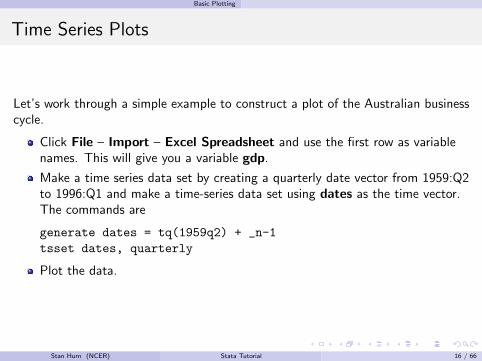
Let’s work through a simple example to construct a plot of the Australian businesscycle.

Click File – Import – Excel Spreadsheet and use the first row as variablenames. This will give you a variable gdp.

Make a time series data set by creating a quarterly date vector from 1959:Q2to 1996:Q1 and make a time-series data set using dates as the time vector.The commands are

generate dates = tq(1959q2) + _n-1

tsset dates, quarterly

Plot the data.


Basic Plotting

Australian GDP


Simple Data Manipulation

Data Transformations

Stata’s basic commands for data transformation are generate and replace.

generate creates a new variable.

replace modifies an existing variable.

Both commands are accessed via the Data menu item on the main Statatoolbar.



generate and replace



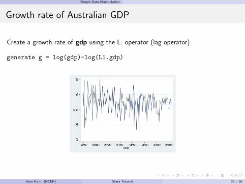
Growth rate of Australian GDP

Create a growth rate of gdp using the L. operator (lag operator)

generate g = log(gdp)-log(L1.gdp)



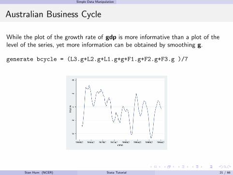
Australian Business Cycle

While the plot of the growth rate of gdp is more informative than a plot of thelevel of the series, yet more information can be obtained by smoothing g.

generate bcycle = (L3.g+L2.g+L1.g+g+F1.g+F2.g+F3.g )/7



Load the food data set

1 Make sure you are in the right working directory (File – Change WorkingDirectory)

2 Load the dataset in food.dta and look at the data characteristics.

3 You can experiment using Statistics – Summaries, tables, and tests –Summary and descriptive statistics but it is simpler to issue the followingcommands from the command window.

describelistbrowsesummarizesummarize food exp, detail



Simple scatter plots

1 Use Grahics – Twoway to create a simple scatter plot of weekly foodexpenditure versus weekly income.

2 Issue the commandtwoway (scatter food exp income)

3 Issue the commandtwoway (scatter food exp income), title(Food Expenditure Data)

4 Issue the commandtwoway (scatter food exp income) (lfit food exp income), title(FittedRegression Line)

The line of best fit is obtained by linear regression of food expenditure on income.We will now explore this in more detail.


Simple Linear Regression

A First Regression

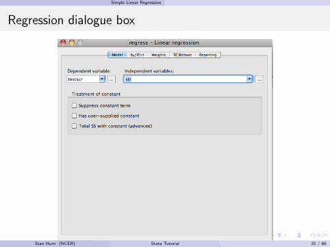
1 Load the data set caschool.dta.

2 Run a regression of the test scores, testscr , against the student-teacher ratio,str . You do this by selecting Statistics – Linear models and related –Linear regression.

3 A dialogue box will pop up which will require you to fill in the dependent andindependent variable.



Regression dialogue box



Regression Results

Stata reports the regression results as follows:

The regression predicts that if class size falls by one student, the test scores willincrease by 2.28 points.



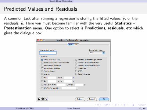
Predicted Values and Residuals

A common task after running a regression is storing the fitted values, y , or theresiduals, u. Here you must become familiar with the very useful Statistics –Postestimation menu. One option to select is Predictions, residuals, etc whichgives the dialogue box



Predicted Values and Residuals

1 Note that the names you choose for the predicted values and/or residualscannot already be taken. Use something obvious like yfit or yhat for thefitted values and res or uhat for the residuals.

2 You can also use the Postestimation option to obtain confidence intervalsfor the prediction using the option Standard errors of the prediction. Savethis as yhatci . The commands. gen yhatu = yhat+1.96*yhatci

. gen yhatl = yhat - 1.96*yhatci

will now generate a 95% confidence interval for the prediction.

3 To be more precise you could use the t-distribution rather than hard-code1.96. The commands are. gen ttail = invttail(e(df_r),0.975)

. gen yhatu = yhat+ttail*yhatci

Note that e(df_r) is the way Stata stores the degrees of freedom for theresiduals and invtttail computes the relevant critical value from thet-distribution.



Predictions with 95% Confidence Interval



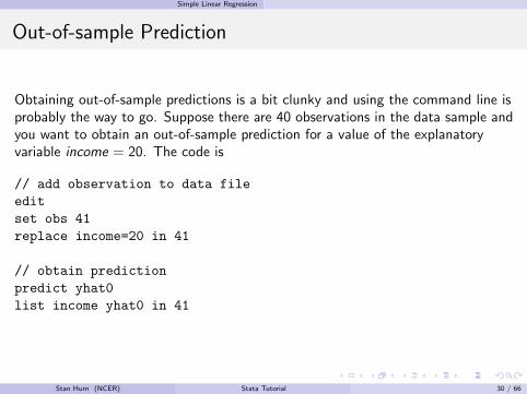
Out-of-sample Prediction

Obtaining out-of-sample predictions is a bit clunky and using the command line isprobably the way to go. Suppose there are 40 observations in the data sample andyou want to obtain an out-of-sample prediction for a value of the explanatoryvariable income = 20. The code is

// add observation to data file

edit

set obs 41

replace income=20 in 41

// obtain prediction

predict yhat0

list income yhat0 in 41



You should explore other visualisation options


Using do files

Using do files

A nice thing about Stata is that there is a simple way to save all your work stepsso you or others can easily reproduce your analysis.

The way to do so is using a so-called do file.

Remember that all Stata does is to execute commands, which you eitherclicked on using the menu or directly typed in the Command window.

A command is just one line of text (or code). If you want to save thiscommand for later use, just copy it (simply click on it in the Review windowand copy the line of text that comes up in the Command window) and pasteit into the do file.

The next slides describe how you can open and use a do file.


Using do files

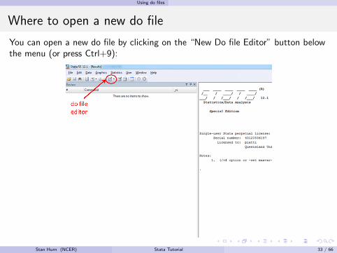
Where to open a new do file

You can open a new do file by clicking on the “New Do file Editor” button belowthe menu (or press Ctrl+9):


Using do files

Using a do file

A do file is just a list of commands. Each command has to start with a new line.Normally you will start your do file telling it which data to load in the first line. Inthe following lines you can then include analysis commands. If you leave a rowempty – no problem. If you want to write comments or text, which are not Statacode, you have to start the row with // or a * symbol; using these symbols tellStata that this line is not to be executed.


Using do files

Executing commands with a do file

If you want to re-run a command from the do file, just highlight the line and pressthe “Execute (do)” button (or press Ctrl+d). If you don’t mark any specific line,Stata will run all the commands in the do file you have currently opened from firstto last. The results of the command(s) are displayed in the main view as if youwere using the menu.


Some Regression Examples Electricity Data

Demand for Residential Electricity

The Excel file elecex.xls has quarterly data on the following variables from1972:02 to 1993:04.

RESKWH = electricity sales to residential customers (million kilowatt-hours)NOCUST = number of customers (thousands)PRICE = electricity tariff (cents/kwh)CPI = consumer price indexINCOME = nominal personal income (millions of dollars)CDD = cooling degree daysHDD = heating degree daysPOP = population (thousands)

Import the data into Stata using the Import wizard. Take care to check the RadioButton asking whether or not to treat the first row as variable names! Once doneyou can save this as elecex.dta for your own convenience.



Time Series Data

Most multiple regression exercises involve data manipulation. This is wherewriting ”do” files is a powerful way of ensuring that you can recover your previouswork and others can reproduce it.

1 This is time series data, so we need to create a date vector set dates as thedate vector.

generate dates = tq(1972q2) + _n-1

tsset dates, quarterly



Data Manipulations

1 Generate the dependent variable:

gen LKWH=log(RESKWH/NOCUST)

2 We want to explain this demand in terms of real per capita income so createthe variable

gen LY=log((100\ast INCOME)/(CPI\ast POP))

3 Another important determinant is price — we want to use the real averagecost of electricity

gen LPRICE=log(100 \ast PRICE/CPI)



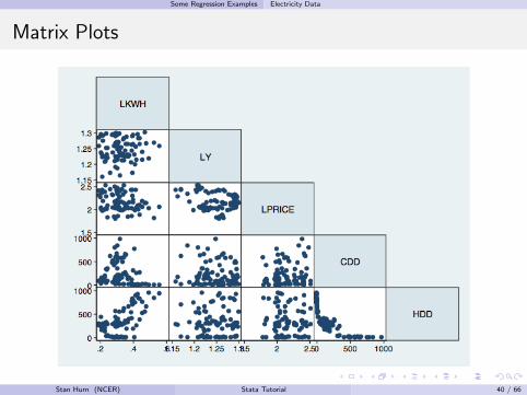
Getting a Feel for the Data

You should always try to understand your data before beginning to model it. Auseful starting point is the Graphics – Scatterplot matrix option. As the namesuggests this creates a matrix of scatterplots of the variables against each other.Hopefully this reveals some pattern to the relationships between the dependentand explanatory variables and no discernible pattern between the explanatoryvariables themselves.



Matrix Plots



Regression Results

The results from running the linear regression of the base model of demand onprice, income and the weather variables are as follows:



ACF and PACF

This is time series data, so one of the problems may be autocorrelation in theresiduals. The autocorrelation function and partial autocorrelation function of theresiduals look as follows



AR(1) Estimation Options

The following dialogue box under the Time Series Prais-Winstein regression allowsyou to correct for autocorrelation in the residuals.



AR(1) output

The results from running the linear regression of the AR(1) model of demand onprice, income and the weather variables are as follows:


Some Regression Examples California Schools Data

California Test Score Data

1 Load the file caschool.dta.

2 Run the regression relating test scores to the student teacher ratio

testscr = β0 + β1str + u

3 The concern is that this equation suffers omitted variable bias which we cancorrect using multiple regression. Try relating test scores to the studentteacher ratio and the percentage of English learners

testscr = β0 + β1str + β2el pct + u

Note that the size of the effect of str is halved!

4 Now try adding expenditure per student to the regression

testscr = β0 + β1str + β2el pct + β3expn stu + u



Presenting Results

This exercise has shown that the coefficient on str in the simple two variablemodel is biased. But the question remains as to how to present this in areasonable way so that we can see the pattern immediately. The answer is to storethe results of the regressions and then to use Stata’s Postestimation menu itemto help organise the presentation of the results.Unfortunately this is going to involve estimating the regressions again and thenusingStatistics – Postestimation – Manage estimation results – Store in memory

After each estimation you will need to name your model. Lets be original and callthem Model1, Model2 and Model3. As you do this, watch how Stata echoes yourcommand and think how easy it would be to use a ”do” file instead.



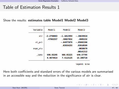
Table of Estimation Results 1

Show the results: estimates table Model1 Model2 Model3

Here both coefficients and standard errors of the various models are summarisedin an accessible way and the reduction in the significance of str is clear.



Table of Estimation Results 2

Further detail on the results: estimates table Model1 Model2 Model3,star(.05 .01 .001)

This is a particularly useful way of summarising the results as the significantcoefficients are marked. Note how str is insignificant in Model 3. Essentially thet-tests on the individual coefficients are interpreted for you!!



Joint Significance Test

Now let’s test the hypothesis that both str and exp stu are zero.The tests are to be found at:Statistics – Postestimation – Tests – Test linear hypotheses

Obviously you are going to have to give Stata some information on whichcoefficients you wish to test. Once you have selected Test linear hypotheses,click on Create and the following dialogue box with appear.



Testing Joint Hypotheses

The result shows that the p-value of the F-test of the joint hypothesis thatβ1 = β3 = 0 is 0.0004 so we would reject the null hypothesis. At least one of strand exp stu is a significant factor in the regression.



Testing Joint Hypotheses for Windows

The result shows that the p-value of the F-test of the joint hypothesis thatβ1 = β3 = 0 is 0.0004 so we would reject the null hypothesis. At least one of strand exp stu is a significant factor in the regression.


Some Regression Examples Food Expenditure and Income

Food Data Set

Study the relationship between food expenditures and incomereg food exp income and plot residuals



Functional Form

It may be that a linear relationship between food expenditures and income isnot a good choice.

Let us try to fit a linear - log model.

food exp = β0 + β1 ln(income) + u

Unfortunately Stata doesn’t recognise ln(income) and you have to generate anew variable, say

gen lincome = log(income)



Fitted Values



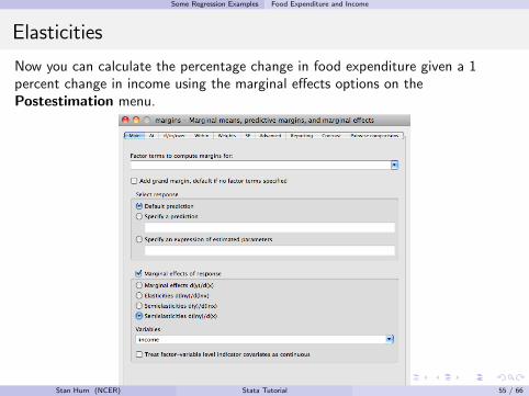
Elasticities

Now you can calculate the percentage change in food expenditure given a 1percent change in income using the marginal effects options on thePostestimation menu.


Instrumental Variables Estimation Wage Data

Wage Data

This example looks at wage data. The datafile is mroz.dta and the focus is onmodelling the wage of married women only. The variables that are important areas follows:

educ = years of schoolingwage = estimated wage from earns., hoursmotheduc = mothers years of schoolingfatheduc = fathers years of schoolingexper = actual labor mkt experlfp = 1 if in labor force, 1975



Estimating a Wage Equation

Suppose we wish to estimate the equation that relates wages to education andexperience:

ln(wage) = β0 + β1educ + β2exper + β3exper 2 + ut .

The problem is that educ may be correlated with u because it is an imperfectproxy for ”ability” and that using OLS may therefore result in biased coefficientestimates.



OLS Results



The IV Estimator

We can now try estimate the regression by IV using mothereduc as an instrumentfor educ . A mother’s education does not itself belong in the daughter’s wageequation, but it is reasonable to propose that more educated mothers are morelikely to have educated daughters.

Click Statistics – Edogenous Covariates – Single-equationinstrumental-variables estimator

This sequence will open a Dialogue Box which will prompt for moreinformation like

1 dependent variable, independent variables, endogenous variables andinstrumental variables;

2 other options for the constant and standard error correction etc.



The IV Estimator



IV Results



Some Observations

1 Although not shown here mothereduc is highly significant in the first-stageregression of the IV estimation indicating it is a strong instrument for educ .

2 The estimated return to education is about 10% lower than the OLSestimate. This is consistent with our earlier theoretical discussion that theOLS estimator tends to over-estimate the effect of a variable if that variableis positively correlated with the omitted factors present in the error term.

3 The standard error on the coefficient on educ is over 2.5 times larger thanthe standard error on the OLS estimate. This reflects the fact that even witha good instrument the IV estimator is not efficient. Of course this situationcan be remedied slightly by adding more valid instruments for educ.


Instrumental Variables Estimation Artificial Data

The Data

The datafile is ivreg2.dta contains 500 artificially generated observations on x , y ,z1 and z2. The variable y is generated as

yt = β0 + β1xt + et , β0 = 3, β1 = 1

withx ∼ N(0, 2) , e ∼ N(0, 1) , cov(x , e) = 0.9 .

Note thatρz1,x = 0.5 ρz2,x = 0.3.



Summary of Estimation Results

Table was generated by using the Postestimation menu option to store resultsand create a table.



Hausman Test

To Implement the Hausman test assuming that you have stored the output fromthe IV and OLS regressions you clickPostestimation – Tests – Hausman specification test



Hausman Test

This indicates a strong rejection of the null hypothesis of exogeneity — indicatingthat cov(x , u) 6= 0 — which we know to be true by construction.


a first tutorial in stata - ncer · a first tutorial in stata ... loading an excel file stan hurn...

Documents