tutorial 03 toppling planar and wedge sliding analysis

Toppling, Planar Sliding, Wedge Sliding 3-1

Toppling, Planar Sliding, Wedge Sliding

This tutorial demonstrates how to perform stability analyses such as toppling, planar sliding and wedge sliding using Dips. The tutorial uses the example file Examppit.dip, which you should find in the Examples folder of your Dips installation folder.

The data has been collected by a geologist working on a single rock face above the first bench in a young open pit mine.

Overall pit slope (45 degrees)

Current floor position

Local bench slopes

The rock face above the current floor of the existing pit has a dip of 45 degrees and a dip direction of 135 degrees. The current plan is to extend the pit down at an overall angle of 45 degrees. This will require a steepening of the local bench slopes, as indicated in the figure above.

The local benches are to be separated by an up-dip distance of 16m. The bench roadways are 4m wide.

Dips v.5.0 Tutorial Manual


Examppit.dip File

First open the Examppit.dip file.

Select: File → Open

Navigate to the Examples folder in your Dips installation folder, and open the Examppit.dip file. Maximize the view.

Figure 1: Examppit.dip data.

The Examppit.dip file contains 303 rows, and the following columns:

• The two mandatory Orientation Columns • A Traverse Column • 5 Extra Columns

Let’s examine the Job Control information for this file.

Job Control

Select: Setup → Job Control



Figure 2: Job Control information for Examppit.dip file.

Note the following:

• the Global Orientation Format is DIP/DIPDIRECTION

• The Declination is 7.5 degrees, indicating that 7.5 degrees will be added to the dip direction of the data, to correct for magnetic declination

• The Quantity Column is NOT used in this file, so each row of the file represents an individual measurement.

Traverses

Let’s inspect the Traverse Information. You can select the Traverses button in the Job Control dialog (the Traverses dialog is also available directly in the Setup menu).

As you can see in the Traverse Information dialog, this file uses only a single traverse:

• The Traverse is a PLANAR traverse, with a DIP of 45 degrees and a DIP DIRECTION of 135 degrees (i.e. the face above the survey bench, as you can read in the Traverse Comment).

• Note that the Traverse Orientation Format is the same as the Global Orientation Format (DIP/DIPDIRECTION), as we would expect for a file with only a single traverse defined.

Select Cancel in the Traverse Information dialog.

Select Cancel in the Job Control dialog.



Pole Plot

Now generate a Pole Plot of the data.

Select: View → Pole Plot

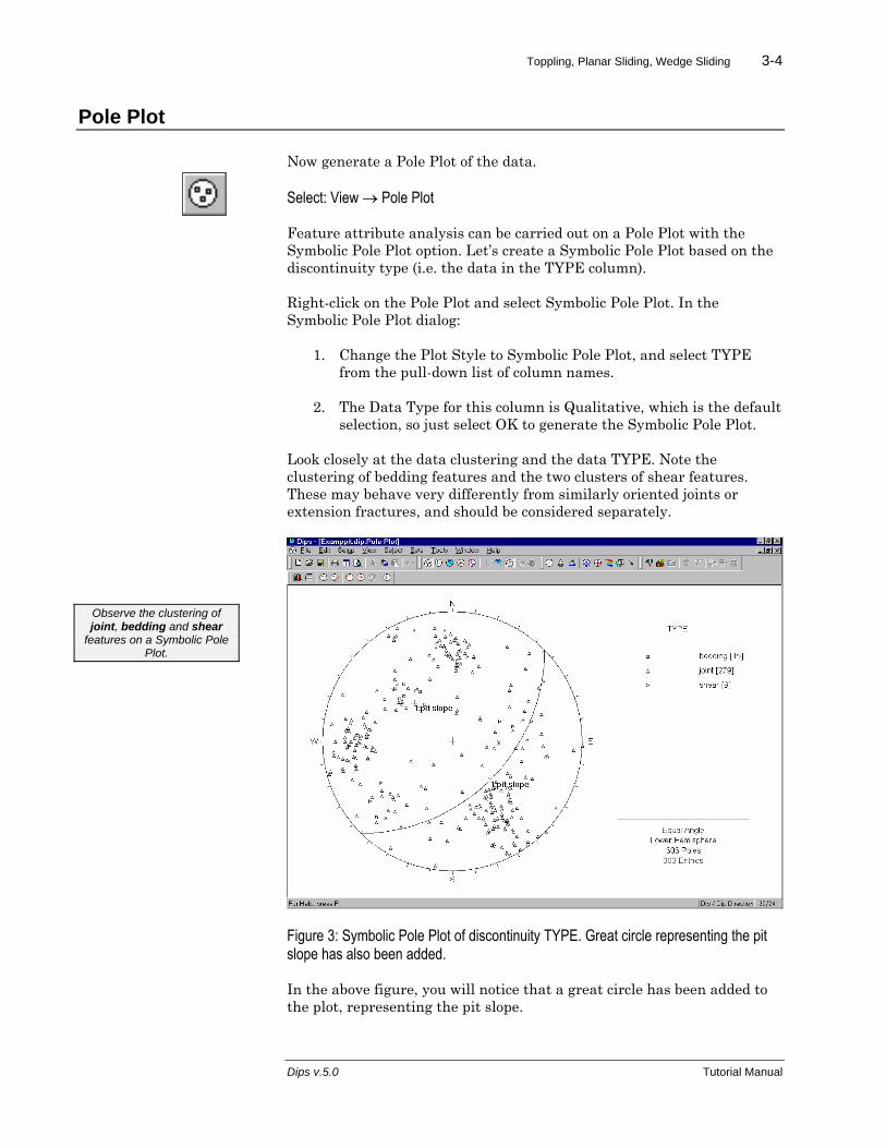
Feature attribute analysis can be carried out on a Pole Plot with the Symbolic Pole Plot option. Let’s create a Symbolic Pole Plot based on the discontinuity type (i.e. the data in the TYPE column).

Right-click on the Pole Plot and select Symbolic Pole Plot. In the Symbolic Pole Plot dialog:

1. Change the Plot Style to Symbolic Pole Plot, and select TYPE from the pull-down list of column names.

2. The Data Type for this column is Qualitative, which is the default selection, so just select OK to generate the Symbolic Pole Plot.

Look closely at the data clustering and the data TYPE. Note the clustering of bedding features and the two clusters of shear features. These may behave very differently from similarly oriented joints or extension fractures, and should be considered separately.

Observe the clustering of joint, bedding and shear

features on a Symbolic Pole Plot.

Figure 3: Symbolic Pole Plot of discontinuity TYPE. Great circle representing the pit slope has also been added.

In the above figure, you will notice that a great circle has been added to the plot, representing the pit slope.



Planes are added to stereonet plots with the Add Plane option, as described below.

Add Plane Before we add the plane, let’s change the Convention. In Dips, orientation coordinates can be displayed in either Pole Vector (Trend/Plunge) format, or Plane Vector format. Right now we want to use the Plane Vector Convention, which for this file is DIP/DIPDIRECTION, since this is the Global Orientation Format.

Use Add Plane to add a great circle representing the pit slope on the stereonet.

To change the Convention, click the left mouse button on the box at the lower right of the Status Bar, which should currently display Trend/Plunge. It should then display Dip / DipDirection. The Convention can be toggled at any time in this manner.

Now let’s add the plane.

Select: Select → Add Plane

1. On the Pole Plot, move the cursor to APPROXIMATELY the coordinates 45 / 135 (Dip / DipDirection). Remember that the cursor coordinates are displayed in the Status Bar.

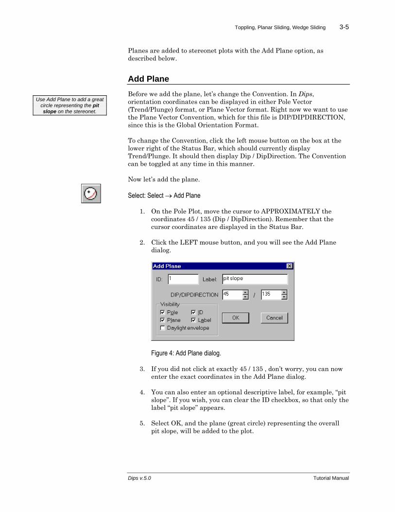
2. Click the LEFT mouse button, and you will see the Add Plane dialog.

Figure 4: Add Plane dialog.

3. If you did not click at exactly 45 / 135 , don’t worry, you can now enter the exact coordinates in the Add Plane dialog.

4. You can also enter an optional descriptive label, for example, “pit slope”. If you wish, you can clear the ID checkbox, so that only the label “pit slope” appears.

5. Select OK, and the plane (great circle) representing the overall pit slope, will be added to the plot.



Contour Plot

Now let’s view the contoured data.

Select: View → Contour Plot

Figure 5: Unweighted Contour Plot of Examppit.dip data.

A useful rule of thumb is that any cluster with a maximum concentration of greater than 6% is very significant. 4-6% represents a marginally significant cluster. Less than 4% should be regarded with suspicion unless the overall quantity of data is very high (several hundreds of poles). Rock mechanics texts give more rigorous rules for statistical analysis of data.

Now let’s apply the Terzaghi Weighting to the data, to account for bias correction due to data collection on the (planar) traverse.

Select: View → Terzaghi Weighting

Observe the change in adjusted concentration for the set nearly parallel to the mapping face (the “bedding plane” joint set).



Observe the effect of bias correction on the bedding plane joint set in particular.

Figure 6: WEIGHTED Contour Plot of Examppit.dip data.

See the Dips Help system for more information about the Terzaghi Weighting procedure used in Dips.

The Terzaghi Weighting option works as a toggle, so re-select the option to restore the original unweighted Contour Plot.

Select: View → Terzaghi Weighting

Contours can be overlaid on a Pole Plot with the Overlay Contours option. Let’s do that now.



Overlay of Contours and Poles

To overlay contours, let’s first view the Pole Plot again.

Select: View → Pole Plot

Note that the Symbolic Pole Plot is still in effect, and does NOT get reset when you switch to viewing other plot types (e.g. the Contour Plot). To overlay contours:

Select: View → Overlay Contours

Let’s change the Contour Mode to Lines, so that the Poles are easier to see.

Select: Setup → Contour Options

In the Contour Options dialog, set the Mode to Lines and select OK.

Figure 7: Overlaid Contours on Pole Plot.

Notice that the Shears in this example are not represented in the contours. This is because the number of mapped shears is small. However, due to the low friction angle and inherent persistence, the shear features may have a dominating influence on stability. It is always important to look beyond mere orientations and densities when analyzing structural data.

Although the SHEARS are not numerous enough to be

represented in the contours, they may have a dominating influence on stability due to

low friction angles and inherent persistence.



Creating Sets

Now use the Add Set Window option to delineate the joint contours, and create four Sets from the four major data concentrations on the stereonet.

Select: Sets → Add Set Window

See the Quick Start Tutorial, the first tutorial in this manual, for instructions on how to create Sets. Also see the Dips Help system for detailed information.

Figure 8: Set Windows formed around the four principal joint sets, using the Add Set Window option.

Note that in Figure 8, the display of the planes was hidden using the Show Planes option. Show Planes can be used at any time to show or hide the planes on any given view.



Failure Modes

We will now proceed with the analysis of 3 potential failure modes of interest – toppling, planar sliding and wedge sliding.

Surface Condition For stability analysis it will be necessary to assume a value for friction angle on the joint surfaces.

For the purpose of estimating a friction angle, we will create a Chart of the data in the SURFACE column of the Examppit.dip file.

Select: Select → Chart

In the Chart dialog, select SURFACE from the pull-down list of columns.

Figure 9: Chart dialog.

For the purpose of our first analysis, which will be a toppling analysis, we are concerned primarily with the joint set at the lower right of the stereonet. Use the Set Filter option in the Chart dialog, to select this Set (in this example, Set ID = 4, yours may be different, depending on the order in which you created the Sets).

Select OK, and the Chart will be created.



View the SURFACE properties and estimate a

friction angle.

Figure 10: Histogram of SURFACE properties for joint set 4.

The joint set illustrated above is predominantly rough (considering both “rough” and “v.rough” features), and so a friction angle of 35 – 40 degrees (a conservative estimate) will be used.

We are finished with the Chart, so close the Chart view and we will return to the stereonet.

Statistical Info We will now add some statistical information to the Pole Plot, by displaying Variability cones around the mean Set orientations. (The shears will be considered separately where appropriate).

If you are still viewing the overlaid Contours on the Pole Plot, toggle this off by re-selecting Overlay Contours.

Select: View → Overlay Contours



Variability Cones

Variability cones are displayed through the Edit Sets dialog.

Select: Sets → Edit Sets

Figure 11: Edit Sets dialog.

For the remainder of this tutorial we will be dealing with WEIGHTED Set information, so select Weighted planes in the Type of Planes pull-down in the Edit Sets dialog.

1. Notice that only the WEIGHTED planes are now listed in the dialog.

2. Select all four planes by selecting the row ID buttons at the left of the dialog. You can click and drag with the mouse, or use the Shift and / or Ctrl keys in conjunction with the mouse, to make multiple selections.

3. Select the Variability checkbox.

4. Select the One Standard Deviation and Two Standard Deviation checkboxes.

5. Select OK.

You now have variability cones representing one and two standard deviations of orientation uncertainty centered on the calculated means.

If you previously toggled the display of planes OFF with the Show Planes option, toggle the display back ON again, by re-selecting Show Planes, since we want to view the Added Plane representing the pit slope.

Select: Select → Show Planes



However, we do not currently want to display the MEAN planes, so let’s toggle their visibility OFF for now. We’ll revisit the Edit Sets dialog.


1. Select ALL planes.

2. Clear ALL Visibility checkboxes (i.e. Pole, Plane, ID and Label).

3. Select OK.

Your screen should look like Figure 12.

Figure 12: Variability cones displayed on Pole Plot.



Toppling A TOPPLING ANALYSIS

using stereonets is based on:

1) Variability cones indicating the extent of the joint set population.

2) A Slip Limit based on the joint friction angle and pit slope.

3) Kinematic considerations.

(The following analysis is based on Goodman 1980. See the reference at the end of this tutorial).

Using the variability cones generated above, proceed with a toppling analysis. Assume a friction angle of 35 degrees, based on the surface condition of the joints (see Figure 10).

Planes cannot topple if they cannot slide with respect to one another. Add a second plane representing a “slip limit” to the stereonet with the Add Plane option.

Select: Select → Add Plane

Position the cursor at APPROXIMATELY 10 / 135 (Dip / DipDirection) and click the left mouse button.

In the Add Plane dialog, if your graphically entered coordinates are not exactly 10 / 135, then enter these exact coordinates and select OK.

NOTE: the DIP angle for this plane is derived from the PIT SLOPE ANGLE – FRICTION ANGLE = 45 – 35 = 10 degrees. The DIP DIRECTION is equal to that of the face (135 degrees). Goodman states that for slip to occur, the bedding normal must be inclined less steeply than a line inclined at an angle equivalent to the friction angle above the slope.

Next, use the Add Cone option to place kinematic bounds on the plot. When specifying cone angles, remember that the angle is measured from the cone axis.

Select: Tools → Add Cone

Click the mouse anywhere in the stereonet, and you will see the Add Cone dialog. Enter the following values:

These values are derived as follows:

• The Trend is equal to the DIP DIRECTION of the face plus 90 degrees (135 + 90 = 225).



• The 60 degree cone angle will place two limits plus / minus 30 degrees with respect to the face DIP DIRECTION as suggested by Goodman – planes must be within 30 degrees of parallel to a cut slope to topple. An earlier 15 degree limit proposed by Goodman was found to be too small.

Select OK on the Add Cone dialog.

The zone bounded by these new curves (outlined in Figure 13 below) is the toppling region. Any Poles plotting within this region indicate a toppling risk. Remember that a near horizontal pole represents a near vertical plane.

The zone outlined in Figure 13 is the toppling

region. Any POLES plotting within this region indicate a

toppling risk.

Figure 13: Toppling risk is indicated by the relative number of poles within joint set which fall within the outlined pole toppling region. Visual estimate indicates about 25 – 30% toppling risk for joint set 4, based on the 95% variability cone.

The two variability cones give a statistical estimate of the toppling risk for the joint set in question. A visual estimate indicates that 25 – 30% of the theoretical population of joint set 4 falls within the toppling zone. It could be said that, ignoring variability in the friction angle, there is an approximate toppling risk of 30%. Frictional variability could be introduced by overlaying additional slip limits corresponding to say 30 and 40 degrees.



Planar Sliding Before we proceed with the Planar Sliding analysis, let’s first delete the cone added for the Toppling analysis.

A PLANAR SLIDING analysis uses Variability Cones, a

Friction cone, and a Daylight Envelope, to test for combined

frictional and kinematic possibility of planar sliding.

Select: Tools → Delete → Delete All

This will delete the cone, and also any Added Text and Arrows which you may have added to the view.

Now, in the Edit Planes dialog, we will:

• delete the “slip limit” plane that we added for the Toppling analysis, and

• display a Daylight Envelope for the pit slope plane.

Select: Select → Edit Planes

Figure 14: Edit Planes dialog.

1. Select the second Added Plane and select Delete.

2. Select the first Added Plane (the Pit Slope), and select the Daylight Envelope checkbox.

3. Select OK.

A Daylight Envelope for the Pit Slope plane should be visible on the stereonet.

A Daylight Envelope allows us to test for kinematics (i.e. a rock slab must have somewhere to slide into – free space). Any pole falling within this envelope is kinematically free to slide if frictionally unstable.



Finally, let’s place a POLE friction cone at the center of the stereonet.


Click the mouse anywhere in the stereonet, and enter the following values in the Add Cone dialog:

Select OK.

Note that the friction angle is equal to our friction estimate of 35 degrees, determined earlier in this tutorial.

Any pole falling outside of this cone represents a plane which could slide if kinematically possible.

The crescent shaped zone formed by the Daylight Envelope and the pole friction circle therefore encloses the region of planar sliding. Any poles in this region represent planes which can and will slide. See Figure 15.



Figure 15: Planar sliding zone is represented by crescent shaped region. Only a small area overlaps the bedding joint set, therefore the risk of planar sliding is minimal.

Again, the variability cones give a statistical estimate of failure probability. Only a small percentage ( < 5 % ) of the bedding joint set falls within this zone.

Planar sliding is unlikely to be a problem.

NOTE: we have been using EQUAL ANGLE projection throughout this analysis. When making visual estimates of clusters and variabilities, it is actually more appropriate to use EQUAL AREA projection to reduce areal distortion and improve visual estimates.

Note that a POLE friction cone angle is measured from the

center of the stereonet.



Wedge Sliding It has been shown that a sliding failure along any of the joint planes is unlikely. However, multiple joints can form wedges which can slide along the line of intersection between two planes.

For this analysis, let’s switch to the Major Planes plot, which allows us to view planes only on the stereonet, without poles or contours.

Select: View → Major Planes

Before we proceed with the Wedge Sliding analysis, let’s first delete the cone added for the Planar Sliding analysis.

Select: Tools → Delete → Delete All

This will delete the cone, and also any Added Text and Arrows which you may have added to the view.

Next, let’s hide the Daylight Envelope for the pit slope, since we do not need it for this analysis.

Select: Select → Edit Planes

In the Edit Planes dialog, select the pit slope plane, and clear the Daylight Envelope checkbox. Select OK.

Next, in the Edit Sets dialog, we want to make the WEIGHTED MEAN planes visible (which we hid earlier in this tutorial), and also hide the Variability cones.


In the Edit Sets dialog, select the four WEIGHTED MEAN planes, and select the Plane visibility checkbox ONLY. Also, clear the Variability Cone and Standard Deviation checkboxes. Select OK.

Finally, let’s add a PLANE friction cone to the stereonet.


Click the mouse anywhere in the stereonet, and enter the following values in the Add Cone dialog:



NOTE: this time we are not dealing with poles but an actual sliding surface or line, so that the friction angle (35 degrees) is taken from the EQUATOR of the stereonet, and NOT FROM THE CENTER as before. Therefore the angle we enter in the Add Cone dialog is 90 – 35 = 55 degrees.

Note that a PLANE friction cone angle is measured from the perimeter (equator) of the

stereonet.

WEDGE SLIDING may occur if the mean joint set

orientation INTERSECTIONS fall within the zone defined by the friction cone and the pit

slope.

Select OK, and your plot should appear as follows:

Figure 16: Major Planes Plot showing WEIGHTED MEAN planes, pit slope and friction cone. Wedge sliding zone is represented by crescent shaped region. Since no plane intersections (black dots) fall within this region, wedge sliding failure should not be a concern.

The zone OUTSIDE the pit slope but enclosed by the friction cone represents the zone of wedge (intersection) sliding. Any plane intersections (highlighted by black dots in Figure 16) which fall within this zone will be unstable. This is not the case in this example, therefore wedge sliding should not be a problem.



Discrete Structures Finally, you should analyze the shear zones mentioned earlier. If these shears occur in proximity to one another they may interact to create local instability.

Perform an analysis similar to the one above using discrete combinations of shear planes.

Using the procedure described above for a wedge

analysis, the stability of discrete combinations of

shear planes, or of shear planes with the mean joint

orientations, may be analyzed.

Examine the stability of other pit slope orientations.

Assume that the joint sets are consistent throughout the

mine property, and perform the analyses described in this

tutorial using 45 degree increments of dip direction

around the pit wall.

• Use the Add Plane option to add planes corresponding to the shear features.

• TIP: while using Add Plane, the Pole Snap option (available in the right-click menu) can be used to snap to the exact orientations of the shear poles.

You should find that the risk of wedge failure along the shear planes is low, for this pit slope configuration.

As a further exercise, determine whether the shears will interact with any of the mean joint set orientations to create an unstable wedge.

Increased Local Pit Slope Repeat these analyses for steeper local slopes. If the overall slope is to be maintained at 45 degrees (see the first page of this tutorial), the local bench slope will have to be increased to accommodate the roadways. What is the critical local slope?

Other Pit Orientations Assume that the joint sets are consistent throughout the mine property. Are there any slope orientations that are more unstable than others? Examine slope dip directions in 45 degree increments around the pit wall.

HINT:

• you can import Dips plots into AutoCAD using the Copy to Metafile option in the Edit menu. This will copy a metafile of the current view to the clipboard, which can then be pasted into AutoCAD.

• Pole or Contour plots showing mean planes and the selected pit slope orientation can be imported into a plan of the pit and placed in their appropriate orientations for quick reference.




References

Goodman, R.E. 1980. Introduction to Rock Mechanics (Chapter 8), Toronto: John Wiley, pp 254-287.

tutorial 03 toppling planar and wedge sliding analysis

Documents