tuning model-based controllers for autonomous maintenance
TRANSCRIPT

Tuning model-based controllers for autonomous maintenance
Citation for published version (APA):Tran, N. Q. (2015). Tuning model-based controllers for autonomous maintenance. Technische UniversiteitEindhoven. https://doi.org/10.6100/IR784454
DOI:10.6100/IR784454
Document status and date:Published: 01/01/2015
Document Version:Publisher’s PDF, also known as Version of Record (includes final page, issue and volume numbers)
Please check the document version of this publication:
• A submitted manuscript is the version of the article upon submission and before peer-review. There can beimportant differences between the submitted version and the official published version of record. Peopleinterested in the research are advised to contact the author for the final version of the publication, or visit theDOI to the publisher's website.• The final author version and the galley proof are versions of the publication after peer review.• The final published version features the final layout of the paper including the volume, issue and pagenumbers.Link to publication
General rightsCopyright and moral rights for the publications made accessible in the public portal are retained by the authors and/or other copyright ownersand it is a condition of accessing publications that users recognise and abide by the legal requirements associated with these rights.
• Users may download and print one copy of any publication from the public portal for the purpose of private study or research. • You may not further distribute the material or use it for any profit-making activity or commercial gain • You may freely distribute the URL identifying the publication in the public portal.
If the publication is distributed under the terms of Article 25fa of the Dutch Copyright Act, indicated by the “Taverne” license above, pleasefollow below link for the End User Agreement:www.tue.nl/taverne
Take down policyIf you believe that this document breaches copyright please contact us at:[email protected] details and we will investigate your claim.
Download date: 17. Jan. 2022

Tuning model-based controllers for autonomous maintenance
PROEFSCHRIFT
ter verkrijging van de graad van doctor aan de Technische Universiteit Eindhoven, op gezag van de rector magnificus prof.dr.ir. C.J. van Duijn,
voor een commissie aangewezen door het College voor Promoties, in het openbaar te verdedigen op donderdag 22 januari 2015 om 16:00 uur
door
Trần Nhật Quang
geboren te Hanoi, Vietnam

Dit proefschrift is goedgekeurd door de promotoren en de samenstelling van de promotiecommissie is als volgt: voorzitter: prof.dr.ir. A.C. Brombacher 1e promotor: prof.dr.ir. A.C.P.M. Backx copromotor: dr. L. Özkan leden: prof.dr. J.M. Maciejowski (University of Cambridge, UK) prof.dr. A.J. Isaksson (Linköping University, Sweden) prof.dr.ir. P.M.J. Van den Hof dr.ir. T.J.J. van den Boom (Technische Universiteit Delft) adviseur: dr.ir. F.A.A. Felici

This work is part of the Autoprofit project, which is funded by theEuropean Union in the Seventh Framework Programme (FP7).
This dissertation has been completed in fulfilment of therequirements of the Dutch Institute of Systems and Control(DISC).
This thesis was prepared using the LATEX typesetting system.Printed by: Gildeprint Drukkerijen, Enschede, the Netherlands.Cover design: Gildeprint Drukkerijen, photo courtesy of Sasol.
A catalogue record is available from the Eindhoven University of TechnologyLibrary.
Tuning model-based controllers for autonomous maintenanceby Tran Nhat Quang. – Eindhoven: Technische Universiteit Eindhoven, 2015.Proefschrift.
ISBN: 978-90-386-3766-2NUR 959
Copyright c©2015 by Tran Nhat Quang.

to my parents,Tung and Phuong

Contents
Summary 1
Acronyms and abbreviations 2
1 Introduction 51.1 Maintenance of model-based controllers . . . . . . . . . . . . . . . . . . 51.2 Problem formulation and approaches . . . . . . . . . . . . . . . . . . . . 111.3 Thesis outline . . . . . . . . . . . . . . . . . . . . . . . . . . . . . . . . . . . . . . 14
2 Model predictive control - Principles and review of tuning approaches 172.1 Introduction . . . . . . . . . . . . . . . . . . . . . . . . . . . . . . . . . . . . . . . 172.2 Model Predictive Control . . . . . . . . . . . . . . . . . . . . . . . . . . . . . . 17
2.2.1 The internal model . . . . . . . . . . . . . . . . . . . . . . . . . . . . . 182.2.2 The disturbance model . . . . . . . . . . . . . . . . . . . . . . . . . . 232.2.3 Receding horizon principle of MPC . . . . . . . . . . . . . . . . . 252.2.4 Tuning and auto-tuning of MPC . . . . . . . . . . . . . . . . . . . 29
2.3 Literature review of MPC tuning and auto-tuning approaches . . . 302.3.1 Engineering rules for selecting the horizons . . . . . . . . . . 302.3.2 Tuning methods . . . . . . . . . . . . . . . . . . . . . . . . . . . . . . . 322.3.3 Auto-tuning methods . . . . . . . . . . . . . . . . . . . . . . . . . . . 39
3 A practical approach to the auto-tuning of MPC 473.1 Introduction . . . . . . . . . . . . . . . . . . . . . . . . . . . . . . . . . . . . . . . 473.2 Preliminaries . . . . . . . . . . . . . . . . . . . . . . . . . . . . . . . . . . . . . . 483.3 Determining the optimum closed-loop bandwidth . . . . . . . . . . . 49

vi
3.3.1 Manual seeking . . . . . . . . . . . . . . . . . . . . . . . . . . . . . . . 493.3.2 Extremum seeking . . . . . . . . . . . . . . . . . . . . . . . . . . . . . 50
3.4 Calculation of the weighting matrices from the closed-loop band-width . . . . . . . . . . . . . . . . . . . . . . . . . . . . . . . . . . . . . . . . . . . . 58
3.5 Implementation on a binary distillation column example . . . . . . 593.5.1 Process description . . . . . . . . . . . . . . . . . . . . . . . . . . . . 593.5.2 Process model . . . . . . . . . . . . . . . . . . . . . . . . . . . . . . . . 613.5.3 Scenarios . . . . . . . . . . . . . . . . . . . . . . . . . . . . . . . . . . . . 633.5.4 Manual seeking . . . . . . . . . . . . . . . . . . . . . . . . . . . . . . . 643.5.5 Extremum seeking . . . . . . . . . . . . . . . . . . . . . . . . . . . . . 71
3.6 Conclusion . . . . . . . . . . . . . . . . . . . . . . . . . . . . . . . . . . . . . . . . 73
4 A reverse-engineering tuning method 774.1 Introduction . . . . . . . . . . . . . . . . . . . . . . . . . . . . . . . . . . . . . . . 774.2 Tuning based on controller matching . . . . . . . . . . . . . . . . . . . . 79
4.2.1 State-space model predictive control . . . . . . . . . . . . . . . 794.2.2 Matching to a one-degree-of-freedom favourite controller 824.2.3 Matching to a two-degree-of-freedom favourite controller 87
4.3 Examples . . . . . . . . . . . . . . . . . . . . . . . . . . . . . . . . . . . . . . . . . 914.3.1 Example 1: Binary distillation column benchmark problem 924.3.2 Example 2: Linear system based on the distillation co-
lumn benchmark . . . . . . . . . . . . . . . . . . . . . . . . . . . . . . 934.4 Conclusion . . . . . . . . . . . . . . . . . . . . . . . . . . . . . . . . . . . . . . . . 97
5 Generalised Predictive Control tuning by controller matching 1015.1 Introduction . . . . . . . . . . . . . . . . . . . . . . . . . . . . . . . . . . . . . . . 1015.2 Preliminaries: Generalised Predictive Control . . . . . . . . . . . . . . 1035.3 Problem formulation . . . . . . . . . . . . . . . . . . . . . . . . . . . . . . . . 108
5.3.1 Matching with no feed-forward control . . . . . . . . . . . . . . 1085.3.2 Matching with feed-forward control . . . . . . . . . . . . . . . . 108
5.4 Matching transfer matrices . . . . . . . . . . . . . . . . . . . . . . . . . . . . 1095.4.1 Matching with no feed-forward control . . . . . . . . . . . . . . 1095.4.2 Matching with feed-forward control . . . . . . . . . . . . . . . . 111
5.5 Finding the weighting matrices . . . . . . . . . . . . . . . . . . . . . . . . . 1125.5.1 Control horizon Hc = 1 . . . . . . . . . . . . . . . . . . . . . . . . . . 1125.5.2 Control horizon Hc > 1 . . . . . . . . . . . . . . . . . . . . . . . . . . 1135.5.3 Scaling KM P C . . . . . . . . . . . . . . . . . . . . . . . . . . . . . . . . . 114
5.6 Example . . . . . . . . . . . . . . . . . . . . . . . . . . . . . . . . . . . . . . . . . . 1155.6.1 Matching with no feed-forward control . . . . . . . . . . . . . . 1165.6.2 Matching with feed-forward control . . . . . . . . . . . . . . . . 119

vii
5.7 Conclusion and future work . . . . . . . . . . . . . . . . . . . . . . . . . . . 125
6 A fresh perspective on the connection between the frequency and fi-nite time domains 1296.1 Introduction . . . . . . . . . . . . . . . . . . . . . . . . . . . . . . . . . . . . . . . 1296.2 Preliminaries and review of relevant developments . . . . . . . . . . 131
6.2.1 MPC based on FIR models . . . . . . . . . . . . . . . . . . . . . . . 1326.2.2 MPC tuning based on the singular values of the Toeplitz
matrix . . . . . . . . . . . . . . . . . . . . . . . . . . . . . . . . . . . . . . 1376.3 New results on the relation between finite time domain and fre-
quency domain . . . . . . . . . . . . . . . . . . . . . . . . . . . . . . . . . . . . 1426.3.1 Asymptotic connection between SVD of the Toeplitz ma-
trix and Bode plot of the open-loop system . . . . . . . . . . . 1436.3.2 Finite-time properties of the Toeplitz and Hankel matrices 1556.3.3 Open issue: Relation between SVD and frequency-domain
properties in finite-time domain . . . . . . . . . . . . . . . . . . . 1586.4 Conclusion and future work . . . . . . . . . . . . . . . . . . . . . . . . . . . 160
7 Industrial validation: FT-depropaniser 1657.1 Introduction . . . . . . . . . . . . . . . . . . . . . . . . . . . . . . . . . . . . . . . 1657.2 The FT-depropaniser . . . . . . . . . . . . . . . . . . . . . . . . . . . . . . . . 166
7.2.1 Process and control structure description . . . . . . . . . . . . 1677.2.2 Base-layer control . . . . . . . . . . . . . . . . . . . . . . . . . . . . . 1697.2.3 APC . . . . . . . . . . . . . . . . . . . . . . . . . . . . . . . . . . . . . . . . 169
7.3 Controller tuning for the FT-depropaniser simulator . . . . . . . . . 1727.3.1 Initial settings . . . . . . . . . . . . . . . . . . . . . . . . . . . . . . . . 1727.3.2 Model . . . . . . . . . . . . . . . . . . . . . . . . . . . . . . . . . . . . . . 1757.3.3 Tuning at commissioning . . . . . . . . . . . . . . . . . . . . . . . . 1767.3.4 Tuning for performance maintenance . . . . . . . . . . . . . . . 179
7.4 Controller tuning for the actual FT-depropaniser . . . . . . . . . . . . 1807.4.1 Initial settings . . . . . . . . . . . . . . . . . . . . . . . . . . . . . . . . 1807.4.2 Model . . . . . . . . . . . . . . . . . . . . . . . . . . . . . . . . . . . . . . 1827.4.3 Tuning at commissioning . . . . . . . . . . . . . . . . . . . . . . . . 1837.4.4 Tuning for performance maintenance . . . . . . . . . . . . . . . 186
7.5 Conclusion . . . . . . . . . . . . . . . . . . . . . . . . . . . . . . . . . . . . . . . . 189
8 Conclusions 1918.1 Contributions . . . . . . . . . . . . . . . . . . . . . . . . . . . . . . . . . . . . . . 1918.2 Future research directions . . . . . . . . . . . . . . . . . . . . . . . . . . . . . 194
Bibliography 196

viii
Appendices 207
A Appendix to Chapter 2 209A.1 Relation between MPC tuning and model uncertainty . . . . . . . . 209A.2 Example: Quadruple tank . . . . . . . . . . . . . . . . . . . . . . . . . . . . . 213
A.2.1 Introduction to the quadruple tank . . . . . . . . . . . . . . . . . 213A.2.2 Effect of model uncertainty on closed-loop performance . 216
B Appendix to Chapter 5 221B.1 Proof of theorem 5.4.1 . . . . . . . . . . . . . . . . . . . . . . . . . . . . . . . . 221B.2 Proof of theorem 5.4.4 . . . . . . . . . . . . . . . . . . . . . . . . . . . . . . . . 227B.3 Proof of theorem 5.5.1 . . . . . . . . . . . . . . . . . . . . . . . . . . . . . . . . 228B.4 Weighting matrices . . . . . . . . . . . . . . . . . . . . . . . . . . . . . . . . . . 230
B.4.1 Matching with no feed-forward control . . . . . . . . . . . . . . 230B.4.2 Matching with feed-forward control . . . . . . . . . . . . . . . . 230
C Appendix to Chapter 6 237C.1 Proof of theorem 6.3.1 . . . . . . . . . . . . . . . . . . . . . . . . . . . . . . . . 237C.2 Proof of theorem 6.3.2 . . . . . . . . . . . . . . . . . . . . . . . . . . . . . . . . 238C.3 Proof of theorem 6.3.3 . . . . . . . . . . . . . . . . . . . . . . . . . . . . . . . . 239C.4 Proof of theorem 6.3.4 . . . . . . . . . . . . . . . . . . . . . . . . . . . . . . . . 241C.5 Proof of theorem 6.3.5 . . . . . . . . . . . . . . . . . . . . . . . . . . . . . . . . 243C.6 Proof of theorem 6.3.7 . . . . . . . . . . . . . . . . . . . . . . . . . . . . . . . . 243

Summary
Tuning model-based controllers for autonomous maintenance
This thesis addresses an unsolved problem, namely the systematic tuning ofmodel-based controllers (model predictive controllers) in order to achieve ahigh-level autonomous model-based operation support system. Despite itspopularity and wide acceptance in the process industry, the performance ofmodel-based controllers degrades over time due to changes in plant dynam-ics or disturbance characteristics resulting even in a complete shutdown ofthe controller by the operators. In addition to model identification, the per-formance degradation of these controllers could be handled up to a certainextent by controller tuning. The first approach considered is a practical auto-tuning method which aims at operating the system at its optimal balance be-tween robustness and disturbance rejection at all times. It brings the closed-loop bandwidth, which is an indication of the balance between robustness andperformance, to the new optimum should any change in the plant dynamicsor disturbance characteristics occur. As frequency-domain characteristics (e.g.closed-loop bandwidth) best represent natural behaviour of linear systems, thenext part of the thesis deals with matching the time-domain tuning parame-ters with a linear time-invariant controller designed in the frequency domain.Controller matching techniques in state-space formulation presented in liter-ature are first investigated and extended, followed by the matching of the Gen-eralised Predictive Control (GPC) with a linear time-invariant controller. Thetuning methods presented are tested on a binary distillation column bench-

2
mark problem and the practical tuning method is further applied to an indus-trial depropaniser. Furthermore, a more direct method to analyse the connec-tion between the frequency and finite time domains is investigated. The long-term objective of this analysis is to pave the way for selecting the weightingmatrices taking into account the characteristics of the plant in the presence ofsystem constraints.

Acronyms and abbreviations
In Table 1, the acronyms and abbreviations used throughout the thesis are spec-ified.

4
Table 1: List of acronyms and abbreviations
Acronym & abbreviation Meaning
APC Advanced Process ControlARX AutoRegressive with eXogenous inputCat Poly Catalytic PolymerisationCV Controlled variableDFT Discrete Fourier transformDCS Distributed Control SystemDV Disturbance variableES Extremum seekingFIR Finite Impulse ResponseFCC Fluid catalytic crackingFSR Finite Step ResponseFT Fischer-TropschGA Genetic AlgorithmGPC Generalised predictive controlIMC Internal model controlLMI Linear matrix inequalitiesLQ Linear quadraticLQR Linear quadratic regulatorLTI Linear time-invariantMIMO Multi-input-multi-outputMPC Model predictive controlMPSSM Minimal Polynomial Start Sequence Markov ParameterMV Manipulated variableOP Opening percentagePID Proportional, integral and derivativePPM Parts per millionPRBS Pseudorandom binary sequencePSO Particle Swarm OptimisationPV Process variableRBS Random binary sequenceRTO Real-time optimisationSCC Synfuels catalytic crackerSISO Single-input-single-outputSP Set-pointSS Steady-stateSVD Singular value decompositionSynfuels Synthetic fuels

1Introduction
1.1 Maintenance ofmodel-based controllers
1.2 Problem formulation andapproaches
1.3 Thesis outline
Carbon emissions, global warming, air pollution, oil spills and dumpinggrounds are just a few words often heard in environmental discussions aroundthe world. Being aware of these issues is everyone’s responsibility. In the fore-front of the campaign to solve such global issues is a good control and optimi-sation strategy for mass production in industry. The process industry, part ofthat broad picture, is the focus of this thesis.
The first chapter of the thesis starts with an overview of the use of controland optimisation technology in the process industry, together with the presentchallenges. Next, we zoom in on a particular part of the multiple-layer controlscheme, which is the advanced process control. Then the problem tackled inthis work is formulated, followed by the structure of the thesis.
1.1 Maintenance of model-based controllers
This section provides an overview of the maintenance of model-based con-trollers, which form an established technology in the process industry. Pro-cess industry is referred to as the manufacturing where chemical change takesplace. Various fields of process industry include the food and beverage, paintsand coatings, chemicals, pharmaceuticals, oil and gas, pulp and paper, steel,glass, cement, etc. The products of these industries are present in every aspect
6 Introduction
of human’s life. The booming of the process industry brings a better and moremodern life to the human being, but it also poses difficult challenges.
Every industry has their own problems to solve and it is not easy to gener-alise about the whole process industry. Nevertheless, common growing con-cerns are the effect of the process industry on the environment and the short-age of natural resources. More and more pressure is put on various sectors toreduce the emission of harmful gases such as greenhouse gases and waste ma-terials that affect the natural balance in the bio-ecosystem. Furthermore, thedecline in the amount of natural resources such as crude oil together with theincrease of the world’s population have forced the process industries to seeknovel technological solutions to the optimisation of their production. This op-timisation involves the maximisation of production rate (i.e. throughput) andminimisation of out-of-production time.
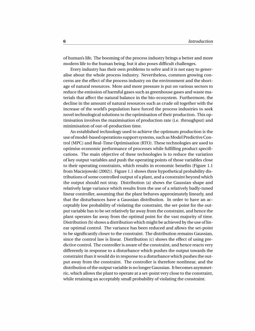
An established technology used to achieve the optimum production is theuse of model-based operations support systems, such as Model Predictive Con-trol (MPC) and Real-Time Optimisation (RTO). These technologies are used tooptimise economic performance of processes while fulfilling product specifi-cations. The main objective of these technologies is to reduce the variationof key output variables and push the operating points of those variables closeto their operating constraints, which results in economic benefits (Figure 1.1from Maciejowski (2002)). Figure 1.1 shows three hypothetical probability dis-tributions of some controlled output of a plant, and a constraint beyond whichthe output should not stray. Distribution (a) shows the Gaussian shape andrelatively large variance which results from the use of a relatively badly-tunedlinear controller, assuming that the plant behaves approximately linearly, andthat the disturbances have a Gaussian distribution. In order to have an ac-ceptably low probability of violating the constraint, the set-point for the out-put variable has to be set relatively far away from the constraint, and hence theplant operates far away from the optimal point for the vast majority of time.Distribution (b) shows a distribution which might be achieved by the use of lin-ear optimal control. The variance has been reduced and allows the set-pointto be significantly closer to the constraint. The distribution remains Gaussian,since the control law is linear. Distribution (c) shows the effect of using pre-dictive control. The controller is aware of the constraint, and hence reacts verydifferently in response to a disturbance which pushes the output towards theconstraint than it would do in response to a disturbance which pushes the out-put away from the constraint. The controller is therefore nonlinear, and thedistribution of the output variable is no longer Gaussian. It becomes asymmet-ric, which allows the plant to operate at a set-point very close to the constraint,while retaining an acceptably small probability of violating the constraint.

1.1. Maintenance of model-based controllers 7
(a)
(b)(c)
Constraint
P (y)
output y
Figure 1.1: Probability density function of a key output; operating point ispushed towards constraints and (c) is the desired operating point.
The development of model-based set-point-pushing control systems hasnow been expanding beyond the process industry. In the semi-plenary talk ofthe 2014 American Control Conference by Dr. Juan de Bedout, the Chief Tech-nology Officer for GE’s Energy Management business, titled "Unlocking Per-formance - How Controls Will Shape The Upcoming Business Landscape", thedevelopment of model-based control technology in cases around infrastruc-ture optimisation including power grid, rail networks, and flight efficiency wasdiscussed. In such large-scale industries, a small improvement in saving re-sources and optimising operation leads to substantial financial benefits. Thatis the reason for the growing development of model-based operations supportsystems.
In the process industry, the model-based operations support systems areimplemented according to a hierarchical control and optimisation scheme asshown in Figure 1.2. This control system aims not only to fulfil the require-ments of the output products, but also to maximise the profits depending onmarket demands, and optimise operating conditions to achieve minimum costsof operation and maintenance. The highest unit of the system, Plant-wide op-timisation, aims to maximise the profit by optimising the use of machines indifferent production facilities, namely answering the questions: when to op-erate and with which resources? It is in fact the scheduling of production intime and space according to the market requirements. Usually the time scale

8 Introduction
of this stage varies from days to months. The next unit, Real-time optimisa-tion, finds the optimal operating points for the processes based on economiccriteria and lasts from hours to days. The third block, Advanced Process Con-trol, is usually a Model Predictive Control, drives the outputs of the process tothe economised set-points determined by the RTO while respecting the systemconstraints and takes minutes to hours. Finally, the input signals from MPC aresent to the base-layer controllers in the Distributed Control System, which areusually the PID controllers. The low-level controllers function at the time scaleof sub-seconds to minutes. The low-level controllers send control signals tothe instrumentation to change the opening percentage of the valves. The focusof this thesis is the Advanced Process Control layer of the hierarchical controlsystem.
The booming of model-based technologies such as advanced process con-trol strongly depends on advances in modelling and identification. The perfor-mance of an APC is largely determined by the quality and maintained calibra-tion of the model. Indeed, the main drawback of model-based technologies,according to Bauer and Craig (2008), is that if left unsupervised, the perfor-mance will deteriorate over time. This degradation can be attributed to thevarying dynamics of the plant, changing disturbance characteristics or otherinstrumentation reasons. The degradation in performance of model-basedcontrol technology gradually happens over time. Such degradation makes sys-tems require maintenance and it makes the technology become difficult for theoperators to work with, if not adequately maintained. The high maintenancecost together with the poor performance often prompt the operators to turn offthe advanced control systems and switch the control to manual mode. In 2005,the following question was posed in Friedman (2005): "Has the advanced pro-cess control industry completely collapsed?". Perhaps not, but there is a realneed for just-in-time maintenance of these model-based control systems, ifone wants to perpetuate the economic benefits of such model-based controlsystems.
The frequent underperformance of model-based control systems has in-spired the creation of the Autoprofit project (Advanced Autonomous Model-Based Operation of Industrial Process Systems), in which the research in thisthesis develops. The target of the project is to maintain the performance andautomate just-in-time maintenance of model-based control systems at a rea-sonable cost. The main philosophy of Autoprofit is based on monitoring, diag-nosing the performance of advanced process control and taking suitable main-taining actions based on economic criteria. The maintenance of advancedprocess control can be divided into two main categories: Re-calibration of themodel and re-tuning of the model-based applications (MPC, RTO and soft sen-

1.1. Maintenance of model-based controllers 9
Plant-Wide Optimisation
Local real-time optimisation (RTO)
Advanced Process Control (APC)
Distributed Control System (DCS)
Plant
Figure 1.2: Hierarchical control structure of processes.
sors). In Annergren et al. (2013), the maintenance scheme of Autoprofit is given(Figure 1.3).
A performance monitoring tool runs online to detect any drop in the per-formance. Once a performance drop is observed, the maintenance procedurefinds out if it is an external factor that causes constraints to be active or aninstrumentation problem. In that case, dedicated maintenance is required tore-establish the performance. If the problem is not attributed to instrumen-tation, the procedure weighs up the cost of a detailed analysis of the problemagainst the potential benefit it can bring. If a detailed analysis is too costly com-pared to the performance loss, the model-based controller is re-tuned in orderto restore the performance, since re-tuning does not need costly excitation of

10 Introduction
Performance drop detected
Base-layer problems or constraint activation due to external cause
Detailed analysis beneficial?
Apply closed-loop diagnosis test
Re-identification beneficial?
Apply closed-loop identification
Tune controller
No
Yes
No
Yes
Yes
Dedicated maintenance
Retune controller
Retune controllerNo
No
Yes
Figure 1.3: Maintenance procedure of model-based control systems.

1.2. Problem formulation and approaches 11
the input signals. If a detailed analysis of the performance drop is beneficial, aperformance diagnosis tool (e.g. the method described in Mesbah et al. (2012))is applied to find out the real cause of the problem. This cause can be a grad-ual change in the system dynamics or a temporary change in the disturbancecharacteristics. This information is used to analyse whether re-identificationof the model is required. If not, re-tuning is used as the solution to the problem.If re-identification is considered beneficial to the lifetime performance of thesystem, a new model is identified using closed-loop identification techniques(Larsson et al. (2013)). A new tuning is then given to the controller with the newmodel.
This thesis tackles the tuning of model-based predictive controllers, whichforms an important part of the maintenance scheme of model-based controlsystems. The model-based predictive controllers are based on solving an op-timisation problem online and their performance is highly dependent on theselection of its cost function. The choice of the weighting matrices in this costfunction is the focus of the thesis.
1.2 Problem formulation and approaches
The aim of MPC systems is to reduce this variance and then to push the keyvariables towards the system constraints so that the system operates closelyto its economically optimal condition. Therefore, the variance of the key vari-ables is a good indication of the performance of the closed-loop system. In ad-dition, the closed-loop performance, the tuning of controllers and the modelaccuracy are inter-related. This relationship has been extensively studied andpresented in robust control theory (Skogestad and Postlethwaite (2005)) us-ing frequency-domain techniques. Define the frequency at which the singularvalues of the sensitivity function of a closed-loop system crosses 0 dB as theclosed-loop bandwidth of the system. It was shown that the performance ofthe closed-loop system becomes sensitive to the model uncertainty at a cer-tain bandwidth. Increasing the bandwidth further beyond the point where themodel accurately describes the actual process dynamics results in closed-loopperformance deterioration. This analysis is depicted in Figure 1.4. It was usedin the tuning of MPC in several works such as Özkan et al. (2012) and Huu-som et al. (2010, 2012). The relation between the closed-loop bandwidth andthe output variance shows that there exists an optimal trade-off between therobustness and the disturbance rejection of the closed-loop system. Detailsof this analysis can be found in Appendix A. Therefore, the question that thisthesis addresses is:"Is it possible to develop structured tuning rules for model-

12 Introduction
Closed-loop bandwidth
Output variance
Too conservative
Too aggressive
Figure 1.4: Relation between closed-loop bandwidth and output variance.
based predictive controllers which allow us to balance closed-loop control per-formance and robustness to model uncertainties in an effective way? Can suchtuning rules be applied in autonomous controller maintenance schemes?".
The existence of an optimal closed-loop bandwidth inspires the two-layertuning approach for this thesis, which is depicted in Figure 1.5. The top layer ofthe approach aims to find the optimal closed-loop bandwidth and the bottomlayer investigates the connection between the time-domain weighting matri-ces and the frequency-domain information of the closed-loop system.
The main question for the top layer of the approach is how to steer the sys-tem to a new optimum bandwidth if changes in plant dynamics or disturbancecharacteristics vary this optimum. To answer this question, two methods areconsidered:
• Manual seeking: starts the tuning with a low closed-loop bandwidth andincreases it until the optimum bandwidth is found.
• Extremum seeking: uses a model-free optimisation method called ex-tremum seeking to keep the closed-loop system at its optimal bandwidthat all times in an autonomous way.
The natural behaviour of linear systems is best described in its natural habi-tat which is the frequency domain. A number of phenomena which are diffi-cult to analyse in the time domain can be investigated in the frequency do-main more easily. For example, the complicated solving of high-order differ-ential equations can be translated into the processing of polynomials with theLaplace transform. The convolution of signals in the time domain is translated

1.2. Problem formulation and approaches 13
into the multiplication in the Laplace domain, which is easier to deal with. Thestability of feedback systems is also well established using frequency-domain-based techniques. With that observation in mind, the main question for thebottom layer is how to develop a tuning method that gives insights into thefrequency-domain properties of the system. To this end, three sub-approachesare investigated:
• Practical approach: The weighting matrices are found by matching thecrossover frequency of the sensitivity function of the MPC (i.e. the closed-loop bandwidth) with a desired one.
• Controller matching: A reverse-engineering tuning method based on Hart-ley and Maciejowski (2011) is also studied. In this thesis, this methodis used to match the MPC with an H∞ controller. The tuning of MPCbecomes the selection of the weighting matrices of the H∞ controller,which gives more insights into the frequency domain. The weighting ma-trices of the H∞ controller are tuned in the top layer of the two-layer tun-ing approach to find the optimum bandwidth. Furthermore, the match-ing of GPC (Generalised Predictive Control) with a favourite controller isalso investigated.
• Investigating the asymptotic and finite behaviour of the Toeplitz matrix:The Toeplitz matrix relates the future inputs and future outputs of MPCin the finite time domain. Any change in the input weighting matricescan be translated into a change in the Toeplitz matrix in the calculationof MPC control inputs. Therefore, investigating this matrix paves the wayfor analysing the connection between the frequency domain and finitetime domain of MPC formulation.
Most of the research in the thesis considers the case where constraints areinactive. In the case of active constraints, the analysis and methods developedbased on the frequency domain are more difficult due to the non-linearity ofthe controller. In that case, the practical auto-tuning method may still be usedbut the optimal trade-off between nominal performance and robustness maynot be the same as in the unconstrained case. Since the system constraintsare usually given in the time domain, the long-term objective of the investiga-tion into the relation between the finite time domain and frequency domain isto tackle the constrained MPC while still keeping track of the dynamics of theclosed-loop system.

14 Introduction
Performance index (output variance)
obtained from measurements
Closed-loop bandwidth ω
Bottom layer:- Practical approach.- Controller matching. Weighting
matrices
Manipulated variables
Top layer:- Manual seeking.- Extremum seeking.
MPC Plant
Measurements
Figure 1.5: Two-layer tuning procedure.
1.3 Thesis outline
The main results of the thesis are presented in the following chapters:
• Chapter 2 presents the main ideas of MPC and reviews different MPCtuning and auto-tuning approaches. The receding horizon principle ofMPC and the computation of its solution are provided. The tuning andauto-tuning methods in literature are categorised and discussed.
• Chapter 3 answers the question relating to the top layer of the two-layerauto-tuning approach. Two sub-approaches, i.e. manual seeking andextremum seeking are considered. When the manual seeking is used, alow-bandwidth setting is taken as the starting point of the tuning pro-cedure. This step is followed by increasing the closed-loop bandwidthwhile monitoring the output variance until the optimum bandwidth isfound. Although the manual seeking method is suitable for commission-ing, restarting the tuning procedure from a low bandwidth is not alwaysnecessary. Therefore, this chapter investigates the use of extremum seek-ing, a model-free optimisation method. The extremum seeking methodenables the system to operate at its optimum bandwidth at all times.When a change in plant dynamics or disturbance characteristics occurs,the method will automatically steer the closed-loop bandwidth to the

1.3. Thesis outline 15
new optimum. In the bottom layer, the practical approach is used in cal-culating the weighting matrices in the cost function of MPC. The weightson the inputs and outputs are computed by matching the crossover fre-quency of the sensitivity function.
• Chapter 4 investigates the use of a reverse-engineering tuning method inthe state space in the bottom layer of the tuning procedure. The reverse-engineering method based on Hartley and Maciejowski (2011) enablesthe MPC to have the same behaviour as an LTI controller, which is alsocalled the favourite controller. In this research, the LTI controller is de-signed by using H∞ techniques. The characteristics of the weightingmatrices of the H∞ controller such as low-frequency gain, crossover fre-quency and high-frequency gain are inherited by the MPC providing thatthe constraints are not active. The weighting matrices of the H∞ con-troller are then used to adjust the closed-loop bandwidth of the MPC.The extension of the method to the case of different control and pre-diction horizons is also presented. This approach in the bottom layeris combined with the manual optimum seeking in the top layer.
• Chapter 5 introduces a tuning method based on controller matching inthe transfer function formulation. The MPC in the transfer function for-mulation is also called the Generalised Predictive Control (GPC). Whereasthe state-space reverse-engineering method uses the observer-based re-alisation of the favourite output-feedback controller, the method pre-sented in this chapter tackles the direct matching in the transfer func-tion formulation. The method also provides the conditions on which thematching is feasible. The infeasibility of the matching shows the limita-tion of the control space that MPC can span with a quadratic cost func-tion.
• Chapter 6 presents a fresh perspective on the relation between the finite-time-domain and frequency-domain characteristics of MPC by lookinginto the Toeplitz matrix, which links the future inputs and future outputsof the system. Initial studies in literature showed the link between thesingular values of the Toeplitz matrix and the gain of the open-loop sys-tem at different frequencies. By replicating the tuning method in Good-win et al. (2005), this chapter shows that this link is not sufficient to drawconclusions about the closed-loop bandwidth of the system. Therefore,the connection between the singular value decomposition of the Toeplitzmatrix and the frequency-domain properties of the system is further anal-ysed. The long-term objective of this analysis is to complete the MPC

16 Introduction
design method based on singular values, which could explicitly take intoaccount the characteristics of the plant in the presence of system con-straints.
• Chapter 7 provides first experimental results of the implementation ofthe practical tuning procedure presented in Chapter 3 on an industrialFT-depropaniser. The experiments are first carried out on a high-fidelityoperator-training simulator of the column and then performed on theactual plant. The results of both sets of experiments are presented to-gether with discussion on suggestions for future experiments.

2Model predictive control - Principles and
review of tuning approaches
2.1 Introduction2.2 Model Predictive Control
2.3 Literature review of MPCtuning and auto-tuningapproaches
2.1 Introduction
This chapter presents the main principles of MPC and a review of the literatureon tuning and auto-tuning of model predictive control systems. Section 2.2introduces common internal models used in MPC prediction, followed by thedisturbance model. The receding horizon principle of MPC is then described.Section 2.3 reviews and categorises different tuning and auto-tuning methodsof MPC.
2.2 Model Predictive Control
Model predictive control (MPC) was initially developed in the seventies by DrJacques Richalet of ADERSA (Richalet et al. (1978)) and Dr Charles Cutler ofShell Oil (Cutler and Ramaker (1980)) and later used as the major advancedprocess control in the hierarchical process control system (Figure 1.2). MPCuses a-priori knowledge of the process system and disturbance characteristicsto predict future process output behaviour. The prediction is used to compute

18 Model predictive control - Principles and review of tuning approaches
the optimum future input manipulations that reduce the variance of the criti-cal outputs, taking into consideration all the signal constraints. Subsequently,the low output variance allows MPC to push the key outputs closer to their op-erating constraints. Unmeasured disturbances and model-plant mismatch arefed back to the controller. The inclusion of measurable signals in the predictionof MPC is its feed-forward part. The implementation scheme of MPC is givenin Figure 2.1. In the following, the principles of MPC are presented. This in-troduction to MPC is based on Maciejowski (2002), Åkesson (2006) and Backx(2008). The internal model used for prediction is first discussed, followed bythe explanation of the receding horizon principle of MPC. This thesis tacklesthe tuning problem of MPC, which is the selection of different parameters ofthe cost function.
Measured disturbances Disturbance
model
Controller:Optimisation and
constraint handling
Process model
∑
Set pointsSet ranges
Constraints
-
Actual process
Model predictive control
∑
Unmeasured disturbances
Controlled variables
Manipulated variables
-
Figure 2.1: Scheme of model predictive control.
2.2.1 The internal model
As mentioned above, MPC uses an internal model of the process and distur-bances to predict future behaviour of the process outputs. A wide variety ofmodel forms is used as the internal model. According to the survey by Qin and
2.2. Model Predictive Control 19
Badgwell (2003), most commercial MPC products are based on linear models.Therefore, in this thesis, we only consider linear model formulations. Thoselinear models include Finite Step Response (FSR), Transfer Function (TF), Fi-nite Impulse Response (FIR), State-Space(SS) and Auto-Regressive with eXoge-nous input (ARX) models.
In MPC commissioning, a linear model is usually obtained from systemidentification. The identification stage in general includes free-run testing,stair-case testing and high-frequency PRBS testing. The free-run testing in-volves monitoring the behaviour of the plant with manipulated variables keptconstant at the operating condition considered. The behaviour of the processoutputs is then completely dependent on the disturbances affecting the plant.By analysing the Fourier transform of the outputs of the free-run tests, one canobtain the open-loop frequency-domain characteristics of the disturbances.The usual behaviour observed in process outputs is low-pass-filtered whitenoise. Properties such as periodic behaviour in open loop can also be obtainedfrom free-run tests. These tests are followed by the so-called stair-case tests,where step changes are applied on different manipulated variables and corre-sponding process outputs are recorded. The stair-case tests provide informa-tion about the steady-state gains and longest time constants of the open-loopsystem. The stair-case tests also provide insights in the range out of which theplant exhibits non-linear behaviour. Finally, the PRBS testing is used to identifythe bandwidth of the plant and its high-frequency characteristics.
Linear models can be divided into three main categories: Non-parametricmodels, semi-parametric models and parametric models. The non-parametricmodels such as Finite Impulse Response (FIR) models or Finite Step Response(FSR) models are not restricted in order and structure. Hence they often havehigh but finite order. Let yk and uk denote the output and input vector of theplant at time instant k , the FIR model is determined by the impulse responseelements Mi of the plant:
y (k ) =N∑
i=0
Mi u (k − i ) (2.1)
where
Mi =
M11(i ) M12(i ) · · · M1m (i )M21(i ) M22(i ) · · · M2m (i )
......
......
Mp 1(i ) Mp 2(i ) · · · Mp m (i )
(2.2)
20 Model predictive control - Principles and review of tuning approaches
p is the number of outputs and m is the number of inputs. The FSR model isdetermined by the step response elements Si of the plant:
y (k ) =N∑
i=0
Si∆u (k − i ) (2.3)
where
Si =
S11(i ) S12(i ) · · · S1m (i )S21(i ) S22(i ) · · · S2m (i )
......
......
Sp 1(i ) Sp 2(i ) · · · Sp m (i )
(2.4)
and∆= 1− z−1. Each parameter Mi j (k ) or Si j (k ) has a unique contribution tothe input-output behaviour. The parameters of the model are mutually inde-pendent. These are the main characteristics of non-parametric models.
Conversely, parametric models have fixed model order and structure. Ex-amples of such models are transfer functions or state-space models. Thesemodels often have a low order. A transfer function model of a discrete-timesystem is given in the z domain:
y (k ) =H (z )u (k ) (2.5)
where
H (z ) =
N11(z )D11(z )
N12(z )D12(z )
· · · N1m (z )D1m (z )
N21(z )D21(z )
N22(z )D22(z )
· · · N2m (z )D2m (z )
......
......
Np 1(z )Dp 1(z )
Np 2(z )Dp 2(z )
· · · Np m (z )Dp m (z )
. (2.6)
Another popular parametric model formulation is the state-space formulation:
x (k +1) = Ax (k ) +B u (k )
y (k ) =C x (k ) +D u (k )(2.7)

2.2. Model Predictive Control 21
where x (k ) is the state vector of the system at time instant k . Many processesare strictly proper, in which case the feed-through term D from the input u (k )to the output y (k ) is 0.
The last type of linear model is the set of semi-parametric models, of whichthe model order is fixed and model structure is non-parametric. The semi-parametric models often have a low order and the order of each input-outputpair is the same. A well-known model of this type is the Minimal PolynomialStart Sequence Markov Parameter model (MPSSM) (Zhu and Backx (1993)).With a fixed order r , the MPSSM model is:
y (k ) =∞∑
i=0
Fi u (k − i ) (2.8)
where Fi =
M0 i = 0Mi 1≤ i ≤ r
r∑
j=1a j Fi− j i > r.
The different model formulations can also be transformed into one an-other. Consider the state-space model (2.7) and assume x (0) = 0. (2.7) resultsin:
z x (k ) = Ax (k ) +B u (k )
y (k ) =C x (k ) +D u (k ).(2.9)
Therefore, x (k ) = (z I −A)−1 B u (k ) and the transfer function from the inputu (k ) to the output y (k ) is given by:
y (k ) =
C (z I −A)−1B +D
u (k ). (2.10)
The impulse response of the system can be derived by writing the transfer func-tion as follows:
y (k ) =
C (z I −A)−1B +D
u (k ) (2.11)
=
C z−1(I − z−1A)−1B +D
u (k ) (2.12)
=
∞∑
i=0
C z−1(z−1A)iB +D
u (k ) (2.13)

22 Model predictive control - Principles and review of tuning approaches
=D u (k ) +∞∑
i=0
C Ai B u (k − i −1). (2.14)
For a stable system, the Markov parameter C Ai B is approximately 0 for i >Nwhere N is the settling time of the system. Therefore (2.14) can be approxi-mated by:
y (k ) =D u (k ) +N∑
i=0
C Ai B u (k − i −1) (2.15)
and the impulse response of the system is given by:
¨
M0 =D
Mi =C Ai−1B for 1≤ i ≤N +1.(2.16)
Assume u (i ) = 0 for i ≤ 0, the relation between the impulse response Mi andstep response Si of the system is obtained by writing:
y (k ) =k∑
i=0
Mi u (k − i ) =M0u (k ) +M1u (k −1) + . . .+Mk u (0) (2.17)
=M0
k∑
j=0
∆u ( j ) +M1
k−1∑
j=0
∆u ( j ) + . . .+Mk∆u (0) (2.18)
=k∑
i=0
Mi∆u (0) +k−1∑
i=0
Mi∆u (1) + . . .+M0∆u (k ) (2.19)
=k∑
i=0
Si∆u (k − i ) (2.20)
where Si =i∑
j=0M j .
The connection between the state-space model and the MPSSM model canbe obtained by using the Cayley-Hamilton theorem:
Theorem 2.2.1 Given a square matrix A and its characteristic equation:
det(A−λI ) =λn +an−1 ·λn−1+ · · ·+a1 ·λ+a0 = 0 (2.21)

2.2. Model Predictive Control 23
then matrix A satisfies:
An +an−1 ·An−1+ · · ·+a1 ·A+a0 · I = 0 (2.22)
The result of the Cayley-Hamilton theorem leads to:
C ·Ai−1 ·
An +an−1 ·An−1+ · · ·+a1 ·A+a0 · I
·B = 0 (2.23)
for i ≥ 1 and therefore:
Mn+i +an−1 ·Mn+i−1+ · · ·+a1 ·Mi+1+a0 ·Mi = 0. (2.24)
The MPSSM model is then obtained by setting r = n .
2.2.2 The disturbance model
The internal model, as formulated in Subsection 2.2.1, often includes a dis-turbance model to take into account the disturbance and noise entering thesystem. As in the case of the model forms, there exists a wide variety of distur-bance models in industrial applications and control theory. In this section, theconstant output disturbance model is discussed. The constant output distur-bance is used in most industrial applications, according to Maciejowski (2002)and Qin and Badgwell (2003). This disturbance model can also be used in thetransfer function formulation as shown in Maciejowski (2002).
With the output disturbance model, the disturbances affecting the systemare modelled as an unknown signal d (k ) added to the outputs of the system,as displayed in Figure 2.2. The constant output disturbance model assumesthat at a time instant k , d (k ) is unknown but an estimate d (k ) can be obtainedby taking the difference between the measured outputs and the predicted out-puts:
d (k ) = y (k )− y (k ). (2.25)
This estimate is assumed to reflect the output disturbance in future time in-stants:
d (k + i ) = d (k ) for ∀i > 0. (2.26)

24 Model predictive control - Principles and review of tuning approaches
Plantu(k) y(k)
d(k)
++
Modelŷ(k) +
-
y(k)-ŷ(k)
Figure 2.2: Output disturbance d (k )
The constant output disturbance can be included in the state-space formula-tion by augmenting the states of the system with an additional state:
x (k +1)d (k +1)
=
A 00 I
x (k )d (k )
+
B0
u (k )
y (k ) =
C I
x (k )d (k )
(2.27)
The constant output disturbance model is included in the FIR model bysimply adding d (k ) = y (k )− y (k ) to the predicted outputs:

2.2. Model Predictive Control 25
y (k +1) =N∑
i=0
Mi u (k − i +1) + d (k )
y (k +2) =N∑
i=0
Mi u (k − i +2) + d (k )
...
(2.28)
In an internal model in the transfer function form, the constant output dis-turbance is modelled as another signal v (k ) passing through a filter with trans-
fer function C (z−1)D (z−1) :
d (k ) =C (z−1)D (z−1)
v (k ) (2.29)
The transfer function model is given by:
y (k ) = z−d B (z−1)A(z−1)
u (k ) +C (z−1)D (z−1)
v (k ) (2.30)
To model the constant output disturbance, we choose the polynomials C (z−1) =1 and D (z−1) = 1−z−1. With these polynomials, (2.29) leads to d (k )−d (k−1) =v (k ). Therefore, if v (k ) is chosen to be 0 for k > 0 and a constant for k = 0, theconstant output disturbance model is achieved.
2.2.3 Receding horizon principle of MPC
As mentioned earlier, MPC uses the internal model of the system to make pre-dictions of the future behaviour of the process outputs. The internal modelused can be of any type discussed in Subsection 2.2.1. In this subsection, thestate-space model is used to illustrate the fundamental idea of MPC, which isthe same for any other model type. The fundamental idea of MPC is the reced-ing horizon principle, presented in Figure 2.3 (Backx (2008)). According to thecontrol scheme in Figure 1.2, MPC receives the operating constraints or set-points from the real-time optimiser. Assume that this set-point is fixed. At thepresent time instant, MPC receives all the measurements of the system. Be-sides the physical measurements, MPC often includes soft sensors, or virtualsensors. These soft sensors collect the physical measurements needed to cal-culate the values of some unmeasurable signals. This calculation is often basedon a first-principles model of the system. All the measurements are used to
26 Model predictive control - Principles and review of tuning approaches
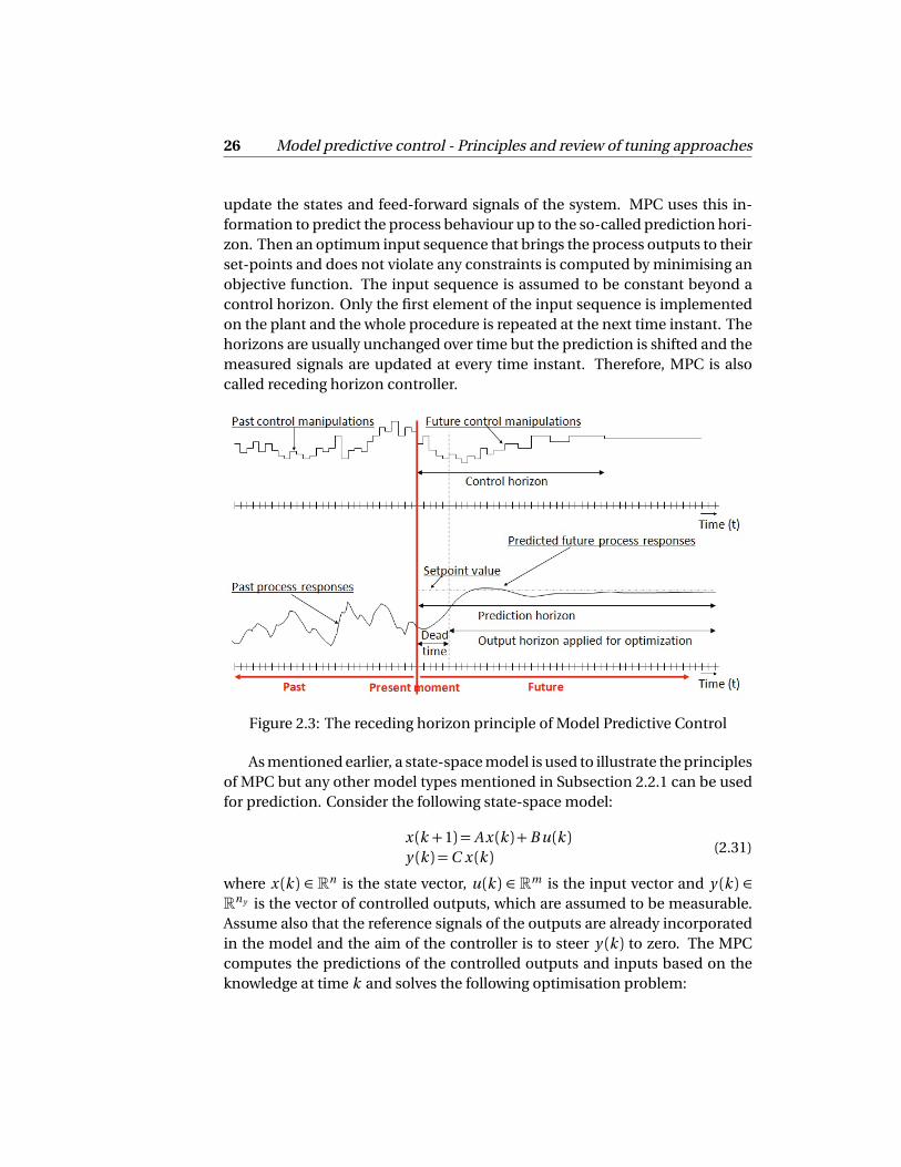
update the states and feed-forward signals of the system. MPC uses this in-formation to predict the process behaviour up to the so-called prediction hori-zon. Then an optimum input sequence that brings the process outputs to theirset-points and does not violate any constraints is computed by minimising anobjective function. The input sequence is assumed to be constant beyond acontrol horizon. Only the first element of the input sequence is implementedon the plant and the whole procedure is repeated at the next time instant. Thehorizons are usually unchanged over time but the prediction is shifted and themeasured signals are updated at every time instant. Therefore, MPC is alsocalled receding horizon controller.
Figure 2.3: The receding horizon principle of Model Predictive Control
As mentioned earlier, a state-space model is used to illustrate the principlesof MPC but any other model types mentioned in Subsection 2.2.1 can be usedfor prediction. Consider the following state-space model:
x (k +1) = Ax (k ) +B u (k )y (k ) =C x (k )
(2.31)
where x (k ) ∈ Rn is the state vector, u (k ) ∈ Rm is the input vector and y (k ) ∈Rny is the vector of controlled outputs, which are assumed to be measurable.Assume also that the reference signals of the outputs are already incorporatedin the model and the aim of the controller is to steer y (k ) to zero. The MPCcomputes the predictions of the controlled outputs and inputs based on theknowledge at time k and solves the following optimisation problem:

2.2. Model Predictive Control 27
min J (k ) =Hp−1∑
i=0
y (k + i |k )
2
Q+
Hu−1∑
i=0
‖∆u (k + i |k )‖2R (2.32)
subject to the constraints on the signals:
yl o w ¶ y (k + i |k )¶ yhi g h
ul o w ¶ u (k + i |k )¶ uhi g h
∆ul o w ¶∆u (k + i |k )¶∆uhi g h
(2.33)
and y (k + i |k ) are the predicted controlled outputs at time k+i and∆u (k + i |k )are the predicted control increments. The use of control increments∆u (k + i |k )instead of the absolute value of u (k + i |k ) gives the controller the integral ac-tion. The weighting matrices Q and R are the weighting matrices, Hp is theprediction horizon and Hu is the control horizon. The cost function J (k ) canthen be written as:
J (k ) = Y (k )>QY (k ) +∆U (k )>R∆U (k ) (2.34)
where
Y (k ) =
y (k |k )y (k +1|k )
...y (k +Hp −1|k )
and∆U (k ) =
∆u (k |k )∆u (k +1|k )
...∆u (k +Hu −1|k )
.
The sequence of predicted outputs Y (k ) are given by:
Y (k ) =Ψ x (k ) + Γu (k −1) +Θ∆U (k ) (2.35)
where
Ψ =
CC AC A2
...C AHp−1
, Γ =
0C B
C AB +C B...
CHp−2∑
i=0Ai B

28 Model predictive control - Principles and review of tuning approaches
Θ =
0 0 · · · 0
C B...
C AB +C B...
... 0
CHu−2∑
i=0Ai B · · · 0
......
CHp−2∑
i=0Ai B · · · C
Hp−Hu−1∑
i=0Ai B .
Let
ξ(k ) =−Ψ x (k )− Γu (k −1) (2.36)
The cost function J (k ) can be expressed as follows:
J (k ) =∆U >H∆U −∆U >G +ξ>ξ (2.37)
where
G = 2Θ>ξ(k )H =Θ>QΘ+R
(2.38)
In the unconstrained case, the solution to the optimisation problem is givenby:
∆U (k ) =
Θ>QΘ+R−1Θ>ξ(k )
=
Θ>QΘ+R−1Θ>
−Γ −Ψ
u (k −1)x (k )
(2.39)
Since only the first element of the solution sequence is implemented, the con-trol law is given by:
∆u (k ) = Ks
u (k −1)x (k )
=
Ks u Ks x
u (k −1)x (k )
(2.40)
where
2.2. Model Predictive Control 29
Ks = [I , 0, ..., 0]
Θ>QΘ+R−1Θ>
−Γ −Ψ
(2.41)
It can be seen that the input signal is in fact a state feedback in the uncon-strained case. In the case that the states of the system are not measurable, astate observer is used to estimate them. The dynamics of the observer are givenby:
x (k +1) = Ax (k ) +B u (k ) +Ko b s
y (k )−C x (k )
(2.42)
where Ko b s is the constant observer gain and y (k ) is the measured output. Ifthe Kalman filter is used, the observer gain Ko b s can be obtained by solvingthe algebraic Riccati equation (Brown and Hwang (1996)). The fact that theunconstrained MPC can be written as a linear output-feedback controller isused to analyse the relation between MPC tuning and model uncertainty, asshown in Appendix A.
2.2.4 Tuning and auto-tuning of MPC
The focus of this thesis is the choice of cost function (2.32), i.e. the tuning prob-lem of MPC. The objective function used in the MPC optimisation problemusually penalises the output and input energy with the weighting matrices Qand R . In general, the parameters that affect the performance of MPC are:
• Control and prediction horizons,
• Weighting matrices,
• Kalman filter gain and disturbance models,
• Reference trajectory.
The selection of these parameters is often referred to in literature as the tuningproblem of MPC. Besides, the auto-tuning methods of MPC deals with the se-lection of the tuning parameters in an autonomous way based on the informa-tion obtained from the measurements. Note that the presence of constraintsalso affects the performance of MPC but the constraints should not be con-sidered as tuning parameters. In the next section, a review of the literature onMPC tuning and auto-tuning approaches is provided.

30 Model predictive control - Principles and review of tuning approaches
2.3 Literature review of MPC tuning and auto-tuning ap-proaches
The principles of MPC show that receding horizon control can be designed invarious ways and the practitioners have much flexibility in designing an MPC.The designer has a large number of options in choosing the model types andthe parameters. This flexibility offers opportunities for selecting a user-friendlyand effective controller. But it also complicates the tuning problem since manyof the parameters have overlapping effects on closed-loop performance androbustness, as stated in Lee and Yu (1994).
Since the tuning of MPC controllers is not a straightforward task, it is worth-while to review the literature that addresses this subject. The review in thissection extends the one given by Garriga and Soroush (2010) and is limited tothe tuning methods of linear MPC. Several of the reviewed articles fix one orseveral parameters and focus their tuning method on the parameters that areconsidered important. Often a parameter is fixed at a value which is prescribedby what the author calls an engineering rule. This review therefore starts with abrief introduction to these engineering rules and proceeds with the other tun-ing methods. It is noteworthy that most of the existing MPC tuning methodsconsider the case of inactive constraints. In this case, simulations are oftenused to assess the performance of the controller when constraints are active.
2.3.1 Engineering rules for selecting the horizons
In general, the engineering rules are applied to the horizons of MPC such asthe prediction horizon Hp and the control horizon Hu . The generally acceptedtuning rule regarding the prediction horizon Hp is that its length needs to coverthe open-loop settling time in samples. This allows the prediction model toinclude all the relevant dynamics of the system.
A common engineering rule for Hp is a value in the range of 80−100% of thesettling time of the slowest subprocess in samples. A few examples that adoptthis approach are Banerjee and Shah (1992), Clarke et al. (1987b), Maurath et al.(1988b), Shridhar and Cooper (1998), Trierweiler and Farina (2003) and Garrigaand Soroush (2008). An exception is the work of Cutler (1983), where Hp =Hu +N , in which N is the settling time of the slowest subprocess in samples.This choice allows the MPC to predict the process output behaviour over a timehorizon needed for the open-loop system to reach steady-state after the lastinput move is applied. In general, a long prediction horizon is used to ensurethat the prediction model covers all the significant dynamics of the system.

2.3. Literature review of MPC tuning and auto-tuning approaches 31
While the engineering rule of choosing a long prediction horizon is gener-ally accepted, ways of selecting the control horizon parameter Hu are rathervaried. A long control horizon requires more computational load since morevariables need to be computed at each time instant. Therefore, to reduce thecomputational load, some works use a default control horizon of 1 (Rani andUnbehauen (1997), Edouard et al. (2005), McIntosh et al. (1989, 1991), Baner-jee and Shah (1992) and Clarke et al. (1987b)). Another advantage of a controlhorizon of 1 is that the input sequence only has one element and therefore theselection matrix
I 0 . . . 0
in MPC solution reduces to an identity matrix,which is invertible. The property is used by a number of works on tuning MPCfor certain favourite properties, such as Shah and Engell (2010, 2011, 2013).
In contrast, some other works propose a longer control horizon that givesMPC degrees of freedom to compute the optimum control input sequence. Forexample, Maurath et al. (1988b) select a control horizon "large enough to ex-tend over all significant adjustments in the manipulated variable needed toimplement a set-point change". Lee and Yu (1994) choose the largest controlhorizon that the computational capacity of the computer system can handle.Cutler (1983) also selects a high Hu such that increasing the control horizonbeyond that value no longer affects the first element of the input sequence.Generally, this value of Hu corresponds to the time in samples for the open-loop system to reach 60% of its steady-state value, Hu =
t60%Ts
. Several works,such as Hinde and Cooper (1994) and Shridhar and Cooper (1998), also fix Hu
at this value.Chapter 7 of Maciejowski (2002) investigates the effect of different selec-
tions of the horizons on MPC when no input penalty is used. According to thatwork, MPC can be equivalent to mean-level control, deadbeat control or theinverse of the plant with different choices of the horizons. Another approachto the selection of Hu is to set Hu equal to the prediction horizon. This is oftenadopted when MPC is designed to match an LQR and achieve infinite horizonbehaviour in the unconstrained case. This selection is found in some works onreverse-engineering tuning methods such as Hartley and Maciejowski (2009,2011, 2013) and Cairano and Bemporad (2010).
While the horizons are often chosen based on engineering rules, the se-lection of the other parameters such as the weighting matrices, disturbancemodels or observer gain is much more varied and each method has its ownadvantages and disadvantages. The focus of this thesis is the selection of theweighting matrices and the disturbance models or observer gain are not in-vestigated in great detail. The combination of real-time optimisation (RTO)and MPC is also not considered. In the following, a review of tuning and auto-tuning methods is provided.

32 Model predictive control - Principles and review of tuning approaches
2.3.2 Tuning methods
There are various tuning methods in literature and in this review, they are di-vided into four main categories:
• Specifications matching methods: The tuning methods falling into thiscategory select the weighting matrices of MPC such that the behaviourof MPC meets certain desired specifications. These specifications canbe given in the time domain or frequency domain.
• Controller matching methods: The MPC tuning parameters are selectedsuch that MPC matches the behaviour of a favourite linear time-invariantcontroller when constraints are inactive.
• Methods based on the conditioning of the control law: Matrix inversionis usually required to compute MPC solution. The conditioning of thatmatrix therefore decides the aggressiveness and robustness of the controlaction. Hence, MPC can be tuned directly by adjusting the matrix thatneeds to be inverted.
• Other pragmatic tuning methods.
Specifications matching methods
There are various ways of defining the desired specifications for the closed-loop system. A favourite behaviour can be determined by the frequency do-main properties of the sensitivity functions or the positions of the closed-looppoles. The desired behaviour can also be defined in the time domain by the set-tling time, level of overshoot, etc. There are two main approaches to matchingthe desired behaviour: By analytical expression or by optimisation. Sometimesa mixture of the two is used.
Iino et al. (1993) compute the complementary sensitivity function of MPCfrom a set of initial tuning parameters. Then the parameters are adjusted suchthat the complementary sensitivity function of the MPC with the new set of pa-rameters meets the robustness requirements. These robustness requirementsare defined by the uncertainty of the plant dynamics∆. When information on∆ is not available, a heuristic choice of the robustness requirements is adopted.
The sensitivity functions of MPC are also used for tuning in Trierweiler andFarina (2003), where the so-called Robust Performance Number (RPN) of thesystem is used as the indication of the performance of the system. This RPNis influenced by both the desired performance of a process and its degree ofdirectionality. It indicates how potentially difficult it is for a given system to

2.3. Literature review of MPC tuning and auto-tuning approaches 33
achieve the desired performance robustly. This method enables the MPC de-signer to specify the desired performance in terms of the complementary sen-sitivity function and to analytically define the matrix weights Q and R . Chiouand Zafiriou (1994) also make use of the complementary sensitivity function infinding the weighting matrices. In this work, these parameters are consideredas optimisation variables of a min-max problem that guarantees the robust sta-bility of the system based on the small gain theorem (Zhou et al. (1996)). Alongthe same lines, Fan and Stewart (2009) also tune the weighting matrices of theMPC based on the small gain theorem and information about the additive un-certainty of the process.
In Bagheri and Sedigh (2013), a desired closed-loop transfer function isgiven to the MPC based on which an analytical expression of the tuning pa-rameters is computed. The method is restricted to first-order-plus-dead-timemodels. This restriction facilitates the computation of the expression of thetuning parameters. This work also shows the feasible regions for the desiredgains, which implies that not any desired behaviour can be matched by theMPC. Along the same lines, Shah and Engell (2010, 2011, 2013) find the weight-ing matrices of GPC by matching the desired closed-loop transfer functions.Shah and Engell (2010) separate the matching of the poles and zeros of the de-sired transfer function and the method is therefore restricted to the SISO case.Shah and Engell (2011, 2013) deal with the MIMO case by minimising the differ-ence between MPC and the controller obtained from the favourite closed-looptransfer function in an optimisation problem. If the resulting error is differentfrom 0, the more important frequency range in the matching will be weightedin the optimisation problem:
min
W− ε−c
2
F(2.43)
where W− is the weighting matrix that defines the important frequency range,
ε−cis the error in frequency domain between the MPC and the achievable con-
troller obtained from the favourite closed-loop specifications, and ‖X ‖F de-notes the Frobenius norm of a matrix X . Furthermore, Shah and Engell (2013)highlight that not any desired behaviour can be achieved by the MPC and pro-pose further methods to choose suitable desired behaviour.
Olesen et al. (2012, 2013) combine the use of frequency and time domainsin their design. The deviation between the controlled outputs and references isthe performance measure of the closed-loop system in the time domain. Thesensitivity function of MPC is used as a measure of robustness in the frequency

34 Model predictive control - Principles and review of tuning approaches
domain. With the use of a performance measure in the time domain and ro-bustness measure in the frequency domain, the tuning approach is supposedto reach a good balance between nominal performance and robustness. Thetuning parameters of MPC are computed from an optimisation problem thatminimises the performance measure and the maximum singular value of thesensitivity function is bounded to guarantee robustness.
In Exadaktylos and Taylor (2010), the weighting matrices are considered asthe optimisation variables of an optimisation problem. The objective functionof this optimisation problem is defined based on the performance specifica-tions. For example, this objective function can be chosen as the deviation ofthe outputs from their references or the difference between the closed-looptransfer function of MPC and a desired transfer function. The method is quitegeneral since one has the freedom to choose the objective function of the op-timisation problem to satisfy multiple performance requirements.
In Garriga and Soroush (2008), the desired specification of the system isdefined by the placement of the closed-loop eigenvalues of the system. A sym-bolic expression for the closed-loop eigenvalues as a function of the weightingmatrices is obtained. It provides insights in how increasing or decreasing onespecific MPC parameter causes the closed-loop eigenvalues to move in a spe-cific direction. It also provides a way of assessing the closed-loop propertiesof an existing MPC controller in terms of closed-loop eigenvalues. It is shownthat as the weights on the magnitude rate of change of the manipulated vari-able are increased, the closed-loop eigenvalues move towards the open-loopeigenvalues, i.e. the closed-loop bandwidth is reduced. The main drawbackof this approach is that the analytical expressions will become too complex tocalculate when the order of the system is high and the prediction horizon islong.
Controller matching methods
This set of tuning methods aim to make the MPC match the behaviour of afavourite controller. The favourite controller is usually a linear time-invariantcontroller. Rowe and Maciejowski (2000a) find the weighting matrices and theobserver gain of MPC for the infinite horizon case such that this MPC matchesan H∞ controller. This H∞ controller is designed using loop-shaping, basedon the normalised left co-prime factorisation as shown in McFarlane and Glover(1992). Along those lines, Rowe and Maciejowski (2000b) try to perform thematching for the finite horizon case without terminal constraints. The favouriterobust controller is designed in the state space formulation and given as a staticstate feedback gain combined with an observer. The matching is performed by

2.3. Literature review of MPC tuning and auto-tuning approaches 35
solving an optimisation problem that minimises the error between the favouritestate feedback gain and the MPC state feedback gain in the unconstrained case.The method was successfully applied to a simple system. However, for a morecomplex system, the optimisation problem may become infeasible or give a lo-cal optimum due to its non-convexity unless a good initial point can be foundfor the optimisation. Maciejowski (2002) proposes a tuning technique basedon "Loop Transfer Recovery", in which a Kalman filter is used in combinationwith the quadratic cost function in an LQ controller. This tuning method gener-alised the one in Lee and Yu (1994) by using a more general disturbance model.
Cairano and Bemporad (2010) discuss the MPC tuning by controller match-ing and present two methods: Optimisation and inverse linear quadratic regu-lator (LQR). The optimisation problem also minimises the error between thefavourite state feedback gain and the MPC unconstrained feedback gain. Amethod to formulate a convex problem with LMI constraints is given. Theinverse LQR is based on the inverse problem of linear optimum control, in-troduced by Kalman (1964) and Anderson and Moore (1971). The tuning byinverse optimality is done with a control horizon equal to the prediction hori-zon together with a terminal weighting matrix, since the unconstrained MPC isequivalent to an LQR. The inverse optimality with respect to an LQR problemis also considered in Chmielewski and Manthanwar (2004) in the framework ofthe minimum variance covariance constrained control problem.
Hartley and Maciejowski (2009, 2011) propose a method to match the MPCto an arbitrary favourite LTI controller. Since the MPC is formulated in statespace, the output feedback LTI controller is decomposed into an observer anda state feedback gain, which is used for the matching. This decomposition isbased on Alazard and Apkarian (1999), in which the set of closed-loop poles arecomputed from the output feedback controller. A number of poles are assignedto the controller and the other poles are assigned to the observer. A commonproblem of this approach is the direct feed-through term from the outputs tothe control inputs in the output feedback favourite controller. The formulationof MPC in state space gives a state feedback control action as shown in (2.40)and this does not allow a direct feed-through from the outputs to the controlinputs. Therefore, loop-shifting methods introduced in Zhou et al. (1996) areused in Hartley and Maciejowski (2009, 2011) to "transfer" the feed-throughterm from the controller to the plant. Hartley and Maciejowski (2013) latersolve this problem by considering the reference tracking LQR in the match-ing. At each time instant, the set-point values of the outputs and inputs arecomputed based on the available information on the feed-through term, thedisturbances and the references. Then those set-point values are included inthe reference tracking LQR. They also present the conditions under which the

36 Model predictive control - Principles and review of tuning approaches
set-point values are the equilibria of the system.
Methods based on the conditioning of the control law
As shown in (2.39), the computation of the MPC solution involves the inver-sion of matrix
Θ>QΘ+R
. Therefore, a measure of the aggressiveness of thecontrol action is the conditioning of this matrix. The MPC controllers formu-lated in other model types invert different matrices in their solutions. How-ever, whatever model type, there is always a strong correlation between theweighting matrices and the matrix to be inverted. Therefore, a number of tun-ing methods investigate the effect of tuning on the conditioning of this matrix.It is called "the system matrix" in Shridhar and Cooper (1997, 1998) and thisname is used in the following.
In order to investigate the conditioning of the system matrix, the singularvalue decomposition (SVD) technique is usually used. Maurath et al. (1988b)have shown that the penalty on the control input of the MPC cost function canbe translated into a change in the singular values of the system matrix. In an ill-conditioned system, a small singular value of the system matrix can contributevery little to reducing the output error while introducing a large control action.In the presence of model-plant mismatch, this large control action may affectthe performance and stability of the system. This problem is also known asthe directionality problem and well-known in, for example, high-purity distil-lation columns and other so-called "stiff" systems. To avoid the conditioningproblem, Maurath et al. (1988b) propose inverting only a number of large sin-gular values of the system matrix and assign the rest to 0. This strategy avoidscontrolling the system in the low-gain direction and provides a certain level ofrobustness.
Shridhar and Cooper (1997, 1998) also investigate the impact of the inputpenalty on the conditioning of the system matrix and arrive at a similar con-clusion. The lower the input penalty, the more ill-conditioned the system ma-trix. Shridhar and Cooper (1997, 1998) approximate the dynamics of the plantto a first-order-plus-dead-time model, in order to compute the analytical ex-pression of the input penalty. This expression is a function of the parametersof the model and the conditioning of the system matrix. Similarly, Doughertyand Cooper (2003) approximate an integrating plant to a first-order-plus-dead-time integrating model to analytically compute the weighting matrices fromthe model parameters and the conditioning of the system matrix. The approx-imation to a simple model in order to obtain an analytical expression of theweighting matrices is also used in Bagheri and Sedigh (2013).
Rojas et al. (2003, 2004) also tune the weighting matrices based on the sin-
2.3. Literature review of MPC tuning and auto-tuning approaches 37
gular values of the system matrix. In those works, the small singular values ofthe system matrix are assigned to zeros such that the input signal satisfies thesystem constraints. Therefore, the advantage of the method is two-fold: it candeal with the system constraints and assure a certain level of robustness. Ro-jas and Goodwin (2004) and Rojas et al. (2004) also show the link between thesingular values of the system matrix and the frequency-domain properties ofthe open-loop system. It has been shown that the singular values of the systemmatrix when zero penalty input is used are exactly the gain of the system overthe frequency range [0;π/Ts ]where Ts is the sampling period. However, the useof this observation in tuning is still an open question.
Pragmatic methods
Maurath et al. (1988a) select the input penalty by trial and error using simu-lation results. This helps to evaluate the aggressiveness of the control action.They suggest initially changing the input penalty by factors of 10. They alsoshow the stability results of MPC for different values of weighting factors andhorizons. Hinde and Cooper (1994) consider first-order-plus-dead-time mod-els and choose a heuristic weighting factor for the input in order to obtain ashort rise time with 10 to 15% overshoot. Nagrath et al. (2000) set the penaltyon input changes to identity and tune the output penalty weights heuristicallyfor their continuous stirred-tank reactor. The weights are selected such that thecontrol action does not behave too aggressively while reference tracking anddisturbance rejection are still guaranteed. Wojsznis et al. (2003) use the ARXmodel of the system to study the effect of the weighting factors on the size of thecontrol moves and on the robustness of the system. They also come to the con-clusion that low penalty on inputs may lead to robustness problems if model-plant mismatch is significant. Based on that observation, an experimental for-mula for the input weighting factor is given to guarantee the robustness of theclosed-loop system. Along those lines, Reverter et al. (2014) also study the ef-fects of the horizons and the input weighting factor on the poles and stabilityof the closed-loop system. From that investigation, a heuristic guideline forchoosing the tuning parameters is given. Drogies and Geest (1999) tune the ref-erence trajectory, the weighting matrices and the horizons heuristically basedon the effect of each tuning parameter on the performance measure. The per-formance measure is defined by the computational load, settling time and risetime. However, a systematic and qualitative tuning method is not presented.An et al. (2009) propose a pragmatic approach to the selection of the weightingmatrices by using the singular values of the controllability and observabilityGramians. The approach hinges on the fact that "the singular values of the

38 Model predictive control - Principles and review of tuning approaches
controllability Gramian correspond to the amount of input energy required tochange the corresponding states" and "the singular values of the observabilityGramian relate to the energy generated by the corresponding states". A prag-matic expression of the weighting matrices is then proposed as a function ofthe singular values of the Gramians.
A number of works deal with the tuning of the Generalised Predictive Con-trol (GPC). Clarke and Mohtadi (1989) show how the horizons and weightingfactors affect the stability of GPC. They suggest choosing an input weight of 0or a small value and augmenting the plant with an auxiliary model to achieverobustness and to perform pole-placement. In this way, the effect of the in-put weight on robustness is small. This tuning approach is applied to a pa-per machine benchmark in Chow et al. (1995). Yoshitani and Hasegawa (1998)heuristically set the input weight to 0.6 in the GPC for their heating furnacein continuous annealing to achieve a satisfactory performance. Karacan et al.(2001) use the default values in Clarke and Mohtadi (1989) for the horizons ofthe GPC and vary the input weight to compare the simulated output error ofthe system at different tuning settings. After the tests, a final value of 1.2 is usedfor experiments on the plant. Yamamoto et al. (2003) fix a long horizon and acontrol horizon of 1 and heuristically choose the input weight based on thecorresponding complementary sensitivity function. The criterion for findinga suitable input weight is based on the small gain theorem (Zhou et al. (1996))and therefore information on the model uncertainty is required. Banerjee andShah (1992) show that by increasing the input weight, the controller is detunedand becomes more sluggish and robust. Therefore, an input weight higher than1 and lower than 2 is proposed to guarantee some level of robustness whileguaranteeing the closed-loop nominal performance.
Conclusion on tuning methods
This section provides an overview of the tuning methods of MPC. The first partof the review introduces the engineering rules for choosing the prediction hori-zon and control horizon. These rules are commonly accepted by many workson tuning MPC. The second part of the review synthesises the methods of se-lecting the weighting matrices in the MPC cost function.
The engineering rules indicate that a long prediction horizon is often se-lected in MPC in order to cover the main dynamics of the system. There is lessagreement on what is the best selection for the control horizon. A short con-trol horizon requires less computational load and a long control horizon meansmore freedom in shaping the future control actions. It also implies that thereare more optimisation variables to compute at each time instant and therefore

2.3. Literature review of MPC tuning and auto-tuning approaches 39
computational time will become critical. However, some works suggest a longcontrol horizon such that increasing it will not affect the first move of the con-trol sequence.
There are many methods for tuning the weighting matrices of MPC. In thisreview, they are divided into four categories: Specifications matching meth-ods, controller matching methods, methods based on the conditioning of thecontrol law and other pragmatic methods. The first category includes tun-ing methods that make sure the closed-loop system meets some desired prop-erties. These properties may be given as the position of closed-loop poles,bounds on the sensitivity or complementary sensitivity functions, or other time-domain behaviour such as the settling time and overshoot.
The controller matching tuning methods, or reverse-engineering tuningmethods, try to match MPC with a favourite LTI controller and when constraintsare inactive, the MPC will inherit the characteristics of the favourite controller.State-space formulation is often used in this type of tuning methods, wherethe static feedback gain of MPC matches that of the favourite controller. Oneobjective of this thesis is to investigate and extend this type of tuning methods.
There are a number of tuning approaches that consider the conditioning ofthe so-called system matrix that is inverted when computing the MPC solution.In these methods, the weighting matrices are connected to the singular valuesof the system matrix. The advantage of these methods is that no optimisationproblem needs to be solved when finding the weighting matrices. Input con-straints can also be dealt with in an explicit way as shown in Rojas et al. (2004).However, the disadvantage of those methods is that the closed-loop propertiesof MPC (such as bandwidth or sensitivity functions) are not explicitly consid-ered. In order to understand the closed-loop characteristics of the MPC basedon singular values, another part of this thesis also looks into the connection be-tween the time-domain system matrix and the frequency-domain properties ofMPC.
Finally, various pragmatic tuning strategies are reviewed. In most of thesemethods, the weighting matrices are chosen based on the general effect of thetuning parameters on the closed-loop performance. In the next part of the lit-erature review, the auto-tuning approaches of MPC are discussed. These ap-proaches aim at finding the weighting matrices of MPC in an autonomous wayand therefore reduce the involvement of engineers and practitioners.
2.3.3 Auto-tuning methods
Auto-tuning of MPC applications is a subject that receives substantial atten-tion of researchers. The main idea of auto-tuning is to select a performance

40 Model predictive control - Principles and review of tuning approaches
index and at each sample time, this performance index is calculated from thelatest measurements. Then the tuning parameters are automatically recom-puted heuristically or by using optimisation techniques, in order to minimisethis chosen performance index. The different choices of optimisation algo-rithms as well as the selection of various performance indices have a consid-erable influence on the efficiency of the auto-tuning method. A scheme of anauto-tuning procedure is given in Figure 2.4.
Performance index obtained from measurements
Weighting matrices
Manipulated variables
Computation of tuning parameters:- Heuristic methods.- Optimisation methods.
MPC Plant
Measurements
Figure 2.4: Scheme of MPC auto-tuning procedure
In McIntosh et al. (1989), three different adaptive tuning strategies for GPCare proposed. The first strategy fixes a control horizon of 1, a zero input weightand the only active tuning parameters is the prediction horizon. The practi-cal choice of the prediction horizon at commissioning is a value between themaximum expected time delay and the settling time of the system. This strat-egy goes against the engineering rules mentioned in Subsection 2.3.1. The sec-ond strategy fixes a long prediction horizon according to the engineering rulesand uses a control horizon equal to the order of the denominator polynomial.In this strategy, the input weight is used as the active tuning parameter. It isstated that this input weight determines the trade-off between nominal per-formance and robustness. The initial input weight is tuned heuristically suchthat the control increment is half the size of the control increment when zeroinput weight is applied. Then it is fine-tuned online to obtain the satisfactory

2.3. Literature review of MPC tuning and auto-tuning approaches 41
response. The third approach considers a zero input weight, fixes the hori-zons at commissioning similarly to the second strategy. This approach sets upthe horizons and weighting matrices of GPC to closely follow certain closed-loop dynamics and adapt these dynamics based on the performance observed.Hasegawa (1994) proposes an adaptive tuning method for GPC by fixing thehorizons and considers the input weight as the tuning parameter. A large in-put weight is set at commissioning to obtain a robust and smooth closed-loopsystem. Then, the input weight is gradually decreased while monitoring thetime-domain output response until a satisfactory performance is obtained.
Al-Ghazzawi et al. (2001) present an auto-tuning method that can improvethe performance of the system as follows: every time the predicted closed-loopresponse is expected to exceed the specification bounds (e.g. ±5% of the set-point value), the auto-tuning algorithm is turned on to adjust tuning param-eters and steer the response into the limits. Two tuning parameters are usedfor this purpose: Weighting matrices on input changes and on outputs (i.e. Qand R , see previous sections). The other parameters such as the control andprediction horizons (Hu and Hp ) are chosen off-line and kept constant. Thismethod is applied to constrained MIMO systems.
The method is based on the linear approximation of the connection be-tween the tuning parameters and the closed-loop time-domain response. Thegradient of the outputs with respect to the tuning parameters ∇x (k )yj are cal-culated recursively:
∂ Y (k +1)∂ x (k )
=M ∗∂ Y (k )∂ x (k )
+N (2.44)
and the linear approximation is given by:
yj (k + i ) = yj (k + i ) +∇x (k )y>j (k + i )∆xk (2.45)
where x (k ) is the tuning parameter at time k , M and N are functions of thetuning parameters and calculated from the system’s data such as the step re-sponse, constraints, etc, Y (k ) = [y (k )...y (k +HN −1)]with HN being the modelhorizon, yj (k+i ) is the j t h output at time instant k+i , yj (k+i ) is the j t h outputat time instant k+i with the new set of tuning parameters,∆xk is the differencebetween the updated and previous tuning parameters. Then, the maximum vi-olation of the prediction is chosen to be minimised. This can be considered asa performance index. Assume that the maximum gap between the referenceand the predicted output occurs at time k +m for output yj , hence an optimi-sation problem is solved to find the optimum tuning parameters:

42 Model predictive control - Principles and review of tuning approaches
min∆xk
‖∇xky >j (k +m )∆xk −∆yj (k +m )‖2 (2.46)
where ∆xk is the change of tuning parameters, ∆yj is the deviation from ref-erence of output yj . The reference is in fact upper and lower bounds in whichthe output of the system must lie. Only the output at time k +m when thegreatest violation of specification occurs is taken into consideration. New tun-ing parameters are found and implemented by solving the problem above. Thismethod is shown to perform better than an off-line tuning method described inShridhar and Cooper (1998), yet produces worse result than an off-line methodwhen the input constraints are active. In that case, the control law becomesconstant and insensitive to the tuning parameters and may lead to performancedegradation, compared to the off-line tuning case.
Another method which concentrates on the time-domain performance ofthe system is proposed in Lee et al. (2008). The approach is grounded in thegenetic algorithm (GA) and fuzzy decision making. According to the authors,this approach is not problem-dependent and can be widely used and adjustedfor different performance purposes. The genetic algorithm is an optimisationalgorithm which creates a search space where it calculates the objective func-tion of each set of tuning parameters (the term "objective function" being usedis the performance index which is mentioned in the beginning of the sectionand not necessarily the cost function of MPC). Then, the algorithm removesthe worst set of tuning parameters and replaces them with the best one. Next,the search space is updated and a new iteration begins. The algorithm stopswhen the number of iteration reaches a pre-defined value.
As far as the application of GA to MPC tuning is concerned, it is combinedwith the multi-objective fuzzy decision making (MOFDM). The latter permitsthe users to define various performance preferences such as the level of over-shoot, the settling time of controlled outputs. Then, the 4-step GA algorithmdescribed in Lee et al. (2008) is applied to find the optimum tuning parame-ters, with the evaluation of performance of each set of tuning parameters be-ing executed using MOFDM. The tuning parameters put into the algorithmare the weighting matrices on the controlled outputs and input changes. Al-though posing a number of performance preferences, the paper does not dealwith model uncertainty or the aggressiveness of the control input, as the per-formance index only covers the overshoot, the deviation of the output from theset-point and the settling time.
Another optimisation approach to finding the tuning parameters is to useParticle Swarm Optimisation (PSO) (Suzuki et al. (2007)). In general, the advan-

2.3. Literature review of MPC tuning and auto-tuning approaches 43
tage of this minimisation technique is that it does not require a differentiableobjective function as it does not calculate the gradient of that function as otherpopular optimisation approaches. In addition, according to the authors, thismethod is easy to use for unskilled operators thanks to its straightforward im-plementation with MPC. Being applied to MPC tuning, this method only tunesthe weighting matrices and fixes the prediction and control horizons. The PSOalgorithm has some features similar to the GA: Both algorithms start with agroup of a randomly generated population, evaluate the population throughthe cost function, update the population and search for the optimum with ran-dom techniques. Both algorithms do not guarantee success.
The PSO technique is used as an optimisation technique to find the tuningparameters and implemented with MPC as shown in Figure 2.4. The PSO usesits own performance index to evaluate the efficiency of tuning parameters:
fi = 1/Gi (2.47)
Gi = (1− e −β )(Es s i +Mp i ) + e −β (ts i − tr i ) (2.48)
Mp i = 100Mp i ma x
yt ma x(2.49)
where β is the weighted coefficient for response and variance property, Es s i isthe steady-state error, ts i is the settling time, tr i is the rising time, Mp i ma x isthe maximum value of yi , yt ma x is the output at the end time. Let m denotethe number of outputs, the optimisation problem is in fact of min-max type:
maxx
min f1, f2, · · · , fm (2.50)
where x is the tuning parameters. The algorithm then computes the optimumtuning parameters and sends them to the MPC. The system sends the outputsto the PSO layer to evaluate the performance index of sets of the tuning pa-rameters. Once the best set is found and the number of iterations reaches apre-defined value, the algorithm stops and the final set of tuning parameters isdetermined. Otherwise, the next iteration begins.
So far, a number of performance indices which take into account variousperformance criteria have been investigated. On the other hand, the cost func-tion of MPC might also be chosen as the performance index for finding the op-timum tuning parameters:
J =Hp∑
j=Hw
‖ y (k + i |k )− r (k + i |k )‖2Q (i )+
Hu−1∑
i=0
‖∆u (k + i |k )‖R (i ) (2.51)
44 Model predictive control - Principles and review of tuning approaches
Liu and Wang (2000) select the performance index in (2.51) and develop anauto-tuning procedure based on multi-objective optimisation. The index isminimised using a trust-region method, varying the following tuning parame-ters: prediction horizon, control horizon, weighting matrix on input changesand on controlled outputs. The method is applied to a kiln dryer and reducesthe oscillations in the controlled output.
There are a number of auto-tuning methods taking robustness of the sys-tem into account. These methods usually include some type of model uncer-tainty in the optimisation problem which finds the tuning parameters. In Hanet al. (2006), the parametric uncertainty model is used, i.e. a number of sys-tem parameters vary within a pre-defined bound. A min-max algorithm is thenused to handle such an uncertainty model:
minPC
maxPG
E I ST W E (PC , PG ) (2.52)
s.t. PC ∈ S and PG ∈ U , where PC is the vector of tuning parameters. In thiscase, these are the prediction, control horizons and the weighting matrix oninput changes. PG is a vector of process model parameters, U is a closed setwhich represents the variation range of model parameters relating to the modeluncertainty, S is the predefined problem space. In the paper, a first-order-plus-dead-time is used to model the system, therefore three varying modelparameters are the gain, the time constant and the delay. Performance indexE I ST W E takes into account the deviations from the set-point of the outputsand the model uncertainty:
E I ST W E =(1+ r (a + b )/S e t p o i n t )
∫ ∞
0
(2.53)
(t n e (t )2+q∆u (t )2)d t +ρH p H u
where e (t ) = r (t )− y (t ), ∆u (t ) denotes the move of manipulated variables, r ,q and ρ are the weights. Minimisation of the maximum performance indexleads to a robust behaviour of the system. The multiplier t n makes the param-eters producing faster time response selected, where n is fixed at 1,2, or 3. Theterm q∆u (t )2 helps avoid dramatic input changes. The term Hp .Hu in the per-formance index moderate the value of the horizons, a is the overshoot of theoutput and b represents the level of oscillation. Therefore, such a performanceindex together with the min-max problem take into account both robustnessand servo behaviour. Then, the min-max problem above is addressed by find-

2.3. Literature review of MPC tuning and auto-tuning approaches 45
ing the maximum of the performance index in the uncertainty bounds and thetuning parameters which bring that maximum index to its minimum value.
In terms of the optimisation algorithm, the advantages of this method aresimilar to those in Suzuki et al. (2007) as both methods use the PSO technique.The main difference of this approach is that it considers the robustness of thesystem. Thus, this approach still results in good performance when model un-certainty occurs. In fact, this is the difference in determining the optimisationproblem as well as the performance index, whereas the optimisation algorithmremains unchanged.
Waschl et al. (2011a,b) choose a performance index that includes both thetracking error and the input energy of the system. At each time instant, theperformance index is updated from the measurements and this informationis used to update the weighting matrices while the horizons are fixed at com-missioning. The special feature of this method is the inclusion of the conditionnumber of the system matrix in the optimisation problem. The condition num-ber is defined as the ratio between the maximum and minimum singular val-ues of a matrix. In the optimisation problem posed by Waschl et al. (2011a,b),the condition number of the system matrix is subject to an upper bound. Thisconstraint is used to make sure that the control action does not become tooaggressive during optimisation.
Conclusion on auto-tuning methods
Overall, most of the auto-tuning methods are based on the optimisation ap-proach where the performance index and the optimisation technique play animportant role. The performance index can be the deviation of the output fromits reference trajectory in the time domain, the peak of the sensitivity functionin frequency domain or a function of different factors as shown above. Somemethods focus on applying optimisation techniques such as PSO or GA to findthe weighting matrices.
The review of tuning and auto-tuning methods show that generally, the in-put weight can be tuned to find a good trade-off between nominal performanceand robustness. In process industry, this optimum is not always obtained dueto various reasons. For example, the tuning setting at commissioning cannotadapt to changes in plant dynamics or disturbance characteristics. With thisobservation in mind, this thesis builds an auto-tuning method whose aim isto find the optimum trade-off between nominal performance and robustnessin an autonomous way. This approach is along the lines of other auto-tuningmethods in literature, in that the objective is to minimise a performance indexusing the tuning parameters. The additional contribution of the proposed ap-

46 Model predictive control - Principles and review of tuning approaches
proach is that it can be used by practitioners to solve the well-known practicalproblem in maintaining MPC systems, which is keeping the balance betweenrobustness and nominal performance. Furthermore, the proposed approachdoes not solely look into the use of an optimisation algorithm in tuning. In-stead, it is based on the actual relation between the weights and the outputvariance as shown in Appendix A, as well as the dynamics of the plant.

3A practical approach to the auto-tuning of
MPC
3.1 Introduction3.2 Preliminaries3.3 Determining the optimum
closed-loop bandwidth3.4 Calculation of the
weighting matrices fromthe closed-loop bandwidth
3.5 Implementation on abinary distillation columnexample
3.6 Conclusion
3.1 Introduction
The purpose of this chapter is to present a practical approach to the two-layerauto-tuning method (Figure 1.5) introduced in Section 1.2 of Chapter 1. In thetop layer, two seeking methods, namely the manual seeking method and theextremum seeking method, are considered to find the optimum bandwidth.The closed-loop bandwidth computed in the top layer is given to the bottomlayer where the tuning parameters are computed. Should any changes in theplant dynamics or disturbance characteristics vary the optimum closed-loopbandwidth, the auto-tuning method will be able to operate the system at itsnew optimum bandwidth. The closed-loop bandwidth is selected to be the op-timisation variable since this is a performance criterion that practitioners andprocess control engineers can relate to. Furthermore, the natural behaviour oflinear systems is well defined in the frequency domain. A tuning method that

48 A practical approach to the auto-tuning of MPC
is related to the closed-loop bandwidth gives more insight into the frequency-domain characteristics of the system. Nevertheless, the auto-tuning methoddescribed in this chapter can also be applied directly to the weighting matriceswithout calculating the closed-loop bandwidths.
Section 3.2 gives the preliminaries of the model and MPC formulation usedin the chapter. Details of the top layer of the auto-tuning method are providedin Section 3.3 and those of the bottom layer are provided in Section 3.4. Theauto-tuning method is implemented on a binary distillation column bench-mark problem in Section 3.5. Section 3.6 concludes the chapter with somecomments and future research openings.
3.2 Preliminaries
Consider a system represented by a discrete-time model of the formx (k +1) = Ax (k ) +B u (k )
y (k ) = C x (k ) (3.1)
where x (k ) ∈ Rnx , u (k ) ∈ Rnu and y (k ) ∈ Rny represent the states, the inputsand the plant outputs of the system. This model is used to compute systempredictions over a finite prediction horizon of Hp samples. The MPC uses thesepredictions to find the input sequence which minimises the cost function givenby:
V (k ) =Hp∑
i=1
ε(k + i |k )Q ε(k + i |k ) +Hu∑
i=1
∆u (k + i |k )R∆u (k + i |k ) (3.2)
where ε(k + i |k ) = y (k + i |k )− r (k + i |k ) ∈Rny is the output error at sample k+i ;∆u (k + i |k ) ∈Rnu is the input increment at sample k+i and Hu is the controlhorizon. Q =Q> > 0 and R =R> > 0 are weighting matrices on the output errorand input increments.
As stated in Chapter 1, the variance of the output error is a good indica-tor for the performance of the closed-loop system. Under the assumption thatµ := E [ε(k )] = 0, the output variance is represented by:
β = E [||ε(k )−µ||2] = E [||ε(k )||2]. (3.3)
A reliable estimate of β depends on the time constant and the characteristicsof the disturbances on the plant. The disturbances affecting the process of-ten have low-frequency characteristics while the measurement noise and mod-elling errors often have high-frequency characteristics. An increase in the closed-loop bandwidthωmp c , corresponding to reducing the penalty on the input en-

3.3. Determining the optimum closed-loop bandwidth 49
ergy, leads to a better rejection of disturbances. This in turn results in a reduc-tion in β . On the other hand, this also renders the controller more sensitiveto modelling errors and measurement noise, which results in an increase ofβ . The optimum bandwidthω∗mp c is the best trade-off between performanceand robustness and results in a minimisation of β . In other words, there existsa functionβ = f (ωmp c ) and this function is known to have an extremum. Sincethis extremum is the balance between disturbance rejection and robustness, itdepends on the characteristics of the disturbance as well as the accuracy of themodel. Any change in the plant dynamics or disturbance characteristics resultsin a change in the optimum closed-loop bandwidth. Details of the auto-tuningmethod to find this optimum are given in the following sections.
3.3 Determining the optimum closed-loop bandwidth
3.3.1 Manual seeking
In the manual seeking, the optimum closed-loop bandwidth is found by man-ually changing the bandwidth and monitoring the output variance. Only theweighting matrices are tuned in the procedure while the horizons are selectedbased on the engineering rules presented in Chapter 1. In addition, based onthe model of the MPC, an initial range for the closed-loop bandwidth can alsobe determined. This range is then divided into a number of linear segments. Aheuristic choice for this number is 10, which proves effective in the simulationdescribed in Section 3.5. Then the 10 bandwidths are considered in the tuningprocedure. Assume that the pre-tests and identification have been performedas described in Subsection 2.2.1 of Chapter 2, the manual seeking method con-sists of the following steps:
1. Initialisation: Determine a certain initial bandwidth from disturbancecharacteristics and available information on modelling errors. The in-formation on disturbance and noise can be obtained by investigatingthe behaviour of the open-loop plant at steady state, while an initial ideaon the frequency range in which the model is correct can be found fromidentification tests. In this method, the initial bandwidth is chosen closeto the bandwidth of the open-loop plant and sent to the bottom layerwhere the weighting matrices are computed and implemented. The out-put variance for this initial bandwidth is then calculated.
2. Seeking: Increase the closed-loop bandwidth to the next value in thebandwidth range. Find the corresponding MPC tuning parameters withthe bottom layer and implement them. Compute the output variance.

50 A practical approach to the auto-tuning of MPC
3. Monitoring: Monitor the output variance. Compare it with the previoustuning. If the variance decreases, keep raising the bandwidth. If it in-creases, the previous tuning is optimal.
If the output variance still decreases at the end of the initial frequency range,the closed-loop bandwidth will be increased until the output variance increases.In other words, a frequency range higher than the robust initial one is consid-ered.
3.3.2 Extremum seeking
Although the relationship between the output variance β and the closed-loopbandwidthωmp c is non-linear and unknown, it is assumed that an extremumβ ∗ = f (ω∗mp c ) exists. This assumption is based on the effect of the closed-loopbandwidth on the output variance described in Appendix A. This is the basisfor using the extremum seeking in the top layer of the auto-tuning method.Furthermore, the manual seeking is not always suitable, especially in the casewhere the optimum bandwidth varies slowly due to gradual change in plantdynamics or disturbance characteristics. In such a case, monitoring the per-formance of the system in the long bandwidth range is not necessary. Instead,moving around the current bandwidth and analysing the performance will givean indication of the location of the new optimum bandwidth. The use of ex-tremum seeking is developed based on this idea.
Introduction to extremum seeking
Extremum seeking is a form of non-model-based adaptive optimisation. It be-longs to the class of gradient-based optimisation techniques and deals withsystems that have an unknown input/output relation, but are known to havean extremum. The basic idea is to perturb the input of the extremum seekingsystem with a so-called dither signal and multiply the extremum seeking sys-tem output (i.e. the output variance of the plant) with the same dither signal.The result of this multiplication gives an estimate of the system’s gradient andthis gradient estimate is used to move the input parameter (i.e. the closed-loopbandwidth) to its extremum, which minimises (or maximises) the output of theextremum seeking system.
The method has existed since the 1920s, has been extensively investigatedin the 1950s and 1960s and has gained renewed interest since the beginningof the new millennium (Stankovic and Stipanovic (2010) and Tan et al. (2010)).It has been used successfully for PID tuning (Killingsworth and Krstic (2006)),
3.3. Determining the optimum closed-loop bandwidth 51
maximum power point tracking of a photo-voltaic system (Levya et al. (2011)),tuning the parameters of mobile sensors (Stankovic and Stipanovic (2010)) andmany other applications (Tan et al. (2010)).
The following introduction to extremum seeking is based on Levya et al.(2011) and Tan et al. (2010). The underlying idea of extremum seeking is il-lustrated in Figure 3.1, which shows the response of a nonlinear function witha global minimum to a sinusoidal perturbation signal around three different
values of x . At x1, ∂ f (x )∂ x
x1
< 0. As a result, the phase of the dither signal in
the output of the nonlinear function is inverted. However, at x3, ∂ f (x )∂ x
x3
>
0, the phase of the dither signal component remains unchanged. Figure 3.1also shows that perturbation around x3 results in a larger amplification of thedither signal, compared to perturbation around x1. Around x2, which is closeto the extremum x ∗, the dither signal is hardly visible in the output, because∂ f (x )∂ x
x2
≈ 0. The amplitude of the output signal β is therefore associated with
the absolute value of the gradient, since
∂ f (x )∂ x
x2
<
∂ f (x )∂ x
x1
<
∂ f (x )∂ x
x3
. (3.4)
Hence, the dither signal component in the output can be regarded as an es-timate of the local gradient around a certain x . This estimate indicates thedirection to seek the optimum. An extremum seeking scheme used to find theoptimum of an unknown nonlinear mapping β = f (x ) is given in Figure 3.2.Extremum seeking tries to estimate the gradient of this nonlinear mapping byperturbing its input x with a periodic dither signal of frequencyωe s and pro-cessing its outputβ . The sinusoidal signal a sin(ωe s k ) is called the dither signaland used in estimating the gradient. In this study, the dither signal is assumedto be a sine wave, although other types of dither signals can be used as well(Tan et al. (2008)).
The mathematical analysis of the extremum seeking algorithm is carriedout by representing β in its first order Taylor expansion, under the conditionthat a << x :
β = f (x ) +∂ f (x )∂ x
a sin(ωe s k ) +O (a 2 sin2(ωe s k )). (3.5)
The first step in the algorithm is processing β by a discrete high-pass filterHH P F (z ). The main function of this filter is to discard any DC component β

52 A practical approach to the auto-tuning of MPC
1 esx a sin(ω k) 2 esx +a sin(ω k) 3 esx +a sin(ω k)
β (x)f
x
Figure 3.1: Response of β to sinusoidal perturbation around various x .
Extremum Seeking
XΣ +
sin(ωesk)
+
HHPF(z)p
HLPF(z)s q
esx a sin(ω k)
x1z
γT- s
NonlinearMap
esβ (x a sin(ω k)) f
X
X
1/a
a
Figure 3.2: Scheme of extremum seeking for an unknown nonlinear map.

3.3. Determining the optimum closed-loop bandwidth 53
that might be present in β , so that the changing of x is solely based on varia-tions in β and not on any DC offset. This filter is designed to only introducea negligible phase shift at frequency ωe s . The filtered output p can be repre-sented by:
p (k ) ' f (x )−β +a∂ f (x )∂ x
sin(ωe s k ). (3.6)
Next, the signal p is multiplied by the dither signal and its output is scaled bya factor 1
a , which results in:
q (k ) '1
a
f (x )−β
sin(ωe s k ) +∂ f (x )∂ x
sin2(ωe s k ). (3.7)
The expression sin2(ωe s k ) can be rewritten, using the trigonometric identity:
sin2(ωe s k ) =1
2−
1
2cos(2ωe s k ). (3.8)
Applying (3.8) to (3.7) results in:
q (k ) '1
2
∂ f (x )∂ x
+1
a
f (x )−β
sin(ωe s k )−1
2
∂ f (x )∂ x
cos(2ωe s k ). (3.9)
Only the first term in (3.9) is of interest. The low-pass filter HLP F (z ) is usedto discard all the harmonics of the dither signal frequency in q , resulting in thefiltered signal:
s (k )'1
2
∂ f (x )∂ x
(3.10)
which is an approximation of the gradient of f (x ). The last step is performedby a discrete-time integrator block that calculates a new x according to:
x (k ) = x (k −1)−γs (k −1) (3.11)
where γ represents the integrator gain. A negative value for s will cause thealgorithm to increase x , while a positive s will result in a decrease of x . If s isclose to zero, x is stable and in the vicinity of the extremum x ∗.
Application of extremum seeking to the auto-tuning method
The ability to find the optimum of an unknown mapping of extremum seek-ing makes it suitable for finding the optimum closed-loop bandwidth in MPC,

54 A practical approach to the auto-tuning of MPC
under the assumption that the function from the closed-loop bandwidth tothe output variance has a global minimum. Not only is the relation betweenthe closed-loop bandwidth and the output variance difficult to obtain analyti-cally in the presence of disturbances and model-plant mismatch, the optimumof this relation is subject to changes due to variation in the plant dynamicsand disturbance characteristics. These changes can also be gradual or dras-tic. Hence, a method that continuously perturbs the closed-loop bandwidth tobring it to the optimum is also capable of steering it to the new optimum if thatoptimum varies over time. Extremum seeking is therefore a suitable method touse in the top layer of the two-layer auto-tuning method. When the extremumseeking method is applied to the auto-tuning approach, the prediction hori-zon is fixed so as to cover the main dynamics of the system, and the controlhorizon is chosen according to the computational capacity of the system. Aschematic overview of the extremum seeking algorithm in the two-layer auto-tuning method is given in Figure 3.3. In the following, the specific design ofeach component in the extremum seeking algorithm in Figure 3.3 is discussed.
ε(k)
Bottom layer: Finding weighting matrices
Top layer: Extremum Seeking
XΣ +
sin(ωeskTs)
+
HHPF(z)HLPF(z)1z
γT- s
X
X
1/a
a
PlantMPCQ and R tuning
u(k)Q & R
2
mpc esω a sin(ω kT ) s
mpcω2
( )ks q p
Measurements
Figure 3.3: Overview of the 2-layer auto-tuning method using extremum seek-ing.
Low-Pass Filter HLP F (z )
As mentioned earlier, the key function of the low-pass filter is to obtain theDC component of (3.9). The fact that the integral of a sinusoid over any integer

3.3. Determining the optimum closed-loop bandwidth 55
multiple of its period is equal to zero can be used to design this low-pass filter:
Te s∫
0
sin(m ·ωe s t )d t = 0 for m ∈N+. (3.12)
A method to obtain the low-pass effect is to calculate the average of q over afull period of the dither signal, Te s =
2πωe s
. The discrete-time representation ofthis filter is:
s (k ) =k∑
n=k−M+1
q (n )≈1
2
∂ f (ωmp c )
∂ ωmp c(3.13)
M =
Te s
Ts+0.5
(3.14)
where bx cdenotes the floor function of x , namely the largest integer not greaterthan x . In practice Te s
Tsmight be a rational number, in that case it needs to be
rounded to the nearest integer to ensure that M ∈N, which is shown in (3.14).Furthermore, it is assumed that Te s >> Ts , which is a valid assumption sinceωe s must be slower than the plant dynamics. This filter has the following z-transform:
HLP F (z ) =M−1∑
n=0
1
Mz−n (3.15)
The structure of (3.15) is that of a low-pass FIR filter. The FIR filter calculatesa sum over M samples at every sampling instant. The structure of (3.15) canbe rewritten into the equivalent IIR structure, which is much more efficient forlarge M and represented by:
HLP F (z ) =1
M
1− z−M
1− z−1(3.16)
and therefore
s (k ) = s (k −1) +1
Mq (k )−
1
Mq (k −M ). (3.17)
Besides removing harmonics of the dither frequency, the low-pass filter has anextra function. It performs the averaging needed to obtain a good estimate ofβ based on samples of ||ε(k )||2. Therefore, a good value of M depends on thedynamics of the process and characteristics of the disturbances. Usually, Mshould be chosen such that the period of the dither signal Te s is 5 to 10 times

56 A practical approach to the auto-tuning of MPC
the open-loop settling time of the process. The -3dB frequency of the low-passfilter is about 2.8/M rad/sample.
High Pass Filter HH P F (z )The objective of the high-pass filter is to remove any DC value present in
(3.5), while introducing little phase distortion at the frequency of interestωe s .A solution that meets both requirements is to use the low-pass filter structureof (3.16) to build a new filter as follows:
HH P F (z ) = 1−HLP F (z ) = 1−1
M
1− z M
1− z−1
=M−1
M − z−1+ 1M z−M
1− z−1(3.18)
and thus
p (k ) = p (k −1) +M −1
Mβ (k )−β (k −1) +
1
Mβ (k −M ). (3.19)
Since the low-pass filter averages the input over Te s , its output is mainly DC.Subtracting this DC value will introduce no phase distortion at the dither fre-quency component if Te s
Ts= M since in that case, the low-pass filter averages
exactly a full period of the dither signal. If Te sTs> M , the averaging misses at
most half a sample; otherwise, if Te sTs<M , the averaging redundantly covers at
most half a sample:
Te s
Ts−M
=
Te s
Ts−
Te s
Ts+0.5
≤ 0.5 (3.20)
This introduces a phase distortion at the dither frequency component of p . Thesignificance of this error can be reflected in the following value:
εm =
Te sTs−M
Te sTs
≤Ts
2Te s(3.21)
Equation (3.21) shows that when Te s goes to infinity, the error in the averaging,denoted by εm , approaches zero. If Te s goes to infinity, so does M , according to(3.14). Despite not being shown here, it is verified that a bigger M also results ina smaller worst-case phase distortion. However, the period of the dither signalcan always be selected to be exactly a multiplication of Ts . The -3dB frequencyof the high-pass filter is about 1.6/M rad/sample.
Equations (3.9) and (3.10) suggest that the high-pass filter is the least im-portant component in the extremum seeking scheme of Figure 3.3, since the

3.3. Determining the optimum closed-loop bandwidth 57
multiplication with the dither signal followed by the low-pass filter eliminatesthe remaining DC term
f (ωmp c )−β
in (3.6).
Both the high-pass and the low-pass filters in the extremum seeking schemeof Figure 3.3 introduce transients at the initialisation of the auto-tuning algo-rithm. During these transients the gradient estimate s given in (3.10) is incor-rect. Therefore, the integrator should only be enabled after these transientshave died out. The duration of the transient introduced by each filter equalsone period of the dither signal Te s , according to (3.15), (3.16) and (3.18). En-abling both filters requires 2Te s for the transient effects to disappear. Whenonly the low-pass filter is active, this time is halved to Te s . This is the reasonwhy the high-pass filter can be omitted in the scheme to increase the speed ofthe seeking.
Dither Frequency ωe s Selecting ωe s is a trade-off between speed of con-vergence and precision. The dither signal should vary slowly enough for theplant to settle and thus preventing the plant dynamics from interfering withthe peak seeking scheme (Krstic and Wang (2000)). On the other hand, increas-ing the dither frequency allows the integrator gain to be increased proportion-ally, while retaining the same domain of attraction (Tan et al. (2006)). As a ruleof thumb, the dither frequency should be slower than the largest relevant fre-quency in the open-loop dynamics of the plant to obtain a useful signal to noiseratio at the input of the extremum seeking scheme. It is worth mentioning thatalthough the exact bandwidth of the plant is unknown, the plant model insidethe MPC system can be used to determine a suitable value forωe s .
Dither Signal Gain a The amplitude of the dither signal is a trade-off be-tween accuracy and precision (i.e. bias and variance). The influence on ac-curacy can be deduced from (3.5), since it shows that by increasing a , the ap-proximation error O (a 2 sin2(ωe s k )) also rises. A larger a will therefore result ina larger offset of ωmp c with respect to ω∗mp c (Tan et al. (2010)). On the otherhand, a smaller a leads to a reduction in precision, as the decrease in the am-plitude of the modulated gradient in (3.5) brings about a deterioration of thesignal-to-noise ratio at the input of the extremum seeking scheme.
Integrator Gain γ The value of the integrator gain is a trade-off betweenspeed of convergence, precision and stability. A higher gain results in fasterconvergence, but the influence of any noise present in the output of the low-pass filter becomes more dominant. Furthermore, there is an upper limit onthe integrator gain with respect to the stability of the adaptation loop. Increas-ing the integrator beyond this value will render the adaptation unstable. The
exact value of this critical value depends on the second derivative,∂ 2 f (ωmp c )∂ ω2
mp c,
which is unknown (Moase et al. (2010)).

58 A practical approach to the auto-tuning of MPC
Extremum Seeking Dither Signal Shape In Tan et al. (2008), it is stated thatwhen using the same extremum seeking parameters, a square wave dither sig-nal results in faster convergence, compared to a sine wave. This is mainly be-cause in that case, the factor 1
2 in (3.10) vanishes. Furthermore, the paper statesthat the domain of attraction and accuracy do not change if both the integratorgain and dither amplitude approach zero. In addition, since a small value of γslows down the convergence of the adaptation loop, which is not desired, theeffect of using a square wave dither signal when γ is close to its critical valuehas to be investigated.
3.4 Calculation of the weighting matrices from the closed-loop bandwidth
Once a desired closed-loop bandwidthωmp c is chosen, there exist several meth-ods to find the corresponding tuning parameters Q and R of MPC. To this end,Rowe and Maciejowski (2000a) adopt the controller matching method in whichMPC is matched to a desired H∞ controller while Lee and Yu (1994) tune theKalman filter and disturbance model to achieve the desired closed-loop band-width.
The weighting factors of the input energy and output energy are correlated.Fixing the input weights and increasing the output weights, or fixing the outputweights and reducing the input weights, both raise the closed-loop bandwidth.Hence, in this work, the input weight is selected as the free variable to adjust theclosed-loop bandwidth. We choose the weighting matrices Q = I and R = ρI ,where I is the identity matrix and ρ is a scalar. In that case, the closed-loopbandwidth is solely determined by the selection of the scalar ρ.
When the constraints are inactive, MPC can be considered to be a lineartime-invariant controller. Therefore, it is possible to derive the sensitivity andcomplementary sensitivity functions of an MPC as in a linear controller in thiscase. In an n ×n system, the sensitivity function has n cut-off frequencies cor-responding to n directions of the system. To find theρ that corresponds to thedesired closed-loop bandwidth ωmp c , the following optimisation problem issolved:
minρ||ωmp c −ωc s (σ1(ρ))||2 (3.22)
whereωc s (σ1(ρ)) is the crossover frequency of the singular value which is mostsensitive to modelling errors of the sensitivity function. The crossover or cut-off frequency of the singular value plot is defined by the lowest frequency at

3.5. Implementation on a binary distillation column example 59
which the singular value crosses 0 dB. As shown in Appendix A, when only onetuning parameter, which is the scalar input penalty, is tuned, increasing thisparameter leads to a decrease in the closed-loop bandwidth and vice versa.This relation can be considered monotonic and therefore, the optimisationproblem above can be assumed convex and solved with a binary search method.For a non-square system, the number of cut-off frequencies of the sensitivityfunction is minnu ; ny where nu is the number of inputs and ny is the numberof outputs. However, the optimisation problem does not change.
3.5 Implementation on a binary distillation column ex-ample
3.5.1 Process description
A binary distillation column benchmark problem is used to illustrate the auto-tuning method in both cases, namely manual seeking and extremum seeking.The purpose of a binary distillation column is to separate two main compo-nents in a feed stream by utilising the difference in the boiling points of thesetwo main components. The operation of a distillation column is based on thefact that volatility decreases when molecular weight increases. Volatility is thetendency of a chemical to vaporise. More details of the functioning of a dis-tillation column and a list of important books on distillation can be found inSkogestad (1997). A simple scheme of a distillation column is given in Figure3.4.
The non-linear model used in this example represents a propane-propylenesplitter, where propane (C3H8) is the heavy component and propylene (C3H6) isthe light component. In the modelling procedure, the relative volatility and theinternal molar flows are assumed to be constant. At each tray, the liquid holdupis constant and the amount of liquid and vapour that comes in is equal to theamount of liquid and vapour that goes out. The main disturbances that affectthe quality of the top and bottom products are the feed rate and feed compo-sition. The measurement of the bottom and top compositions is assumed tosubject to white noise. The characteristics of the plant are:
• The plant output consists of two variables, namely the top and bottomcompositions of the light component in the distillation column.
• The operating condition of the column is a top composition of 0.95 [molefraction] and a bottom composition of 0.05 [mole fraction]. The corre-sponding liquid and vapour flows are 521 Kmol/min and 664 Kmol/min,

60 A practical approach to the auto-tuning of MPC
Boilup (vapour)
Reboiler
Bottom (liquid)
Steam
Cooling water
Condenser
Distillate (liquid)Reflux (liquid)Liquid flow
Vapour flow
Feed (liquid)
Figure 3.4: Scheme of a distillation column.
respectively.
• An LV (Liquid-Vapour) control configuration is considered, hence the re-flux (liquid) flow rate and reboiler (vapour) flow rate are the manipulatedvariables (Skogestad (1997)).
• The feed rate and feed composition are considered as unmeasured dis-turbances and modelled by low-pass filtered white noise. This assump-tion is realistic as the feed comes from upstream processes with low-passcharacteristics.
• The sampling time Ts of the measurement is 5 minutes. Since the timeconstant of the slowest and dominant dynamics of the process is about50 minutes, the sampling time is therefore chosen 5 minutes, which is1/10 of the most relevant time constant. In practice, this sampling timecan be smaller as shown in the industrial validation in Chapter 7.
Specific parameters of the distillation column are given in Table 3.1.

3.5. Implementation on a binary distillation column example 61
Table 3.1: Details of distillation column model
Description Value UnitsNumber of trays 110Feed location 39Relative volatility 1.35Feed rate 215 [Kmol/min]Feed liquid fraction 1Feed composition 0.65 [mole fraction]Molar holdup 30 [Kmol]
3.5.2 Process model
The column is controlled with an LV-configuration, in which the liquid andvapour flows are MV’s, the top and bottom compositions are CV’s and the feedrate and feed composition are unmeasured disturbances.
The operating point is considered as the steady-state condition of the col-umn and the model of the column reflects the relation between the deviation ofthe inputs from their steady state condition values and that of the outputs fromtheir steady-state values. A linear model is identified by exciting the deviationof liquid and vapour flows from the operating points with white noise signals.The standard deviation of these white noise signals is 10 [Kmol/min]. The feedrate and feed composition are assumed to be filtered white noise whose stan-dard deviations are 8 [Kmol/min] and 0.05 [mole fraction], respectively. Thebandwidth of their low-pass filters is π/100 [rad/min]. The measurement ofthe outputs is subject to white noise whose standard deviation is 0.01 [molefraction].
The transfer function of the model is given by:
d yb o t
d yt o p
=
0.001357z−0.0009633z 2−1.528z+0.5679
−0.0009023z+0.000597z 2−1.528z+0.5679
0.001174z−0.0009952z 2−1.528z+0.5679
−0.0003762z+0.0002929z 2−1.528z+0.5679
d Ld V
(3.23)
where d yb o t and d yt o p are the deviation of the bottom and top compositionsfrom the operating points, d L and d V are the deviation of the liquid and vapourflows from the operating points, respectively. The step response of the modelis given in Figure 3.5. It shows that the settling time of the column is approx-imately 200 minutes. In the LV-configuration, an increase in the liquid flowwith a constant vapour flow results in purer top product and an increase in thetop composition. It also leads to more light component at the bottom, which

62 A practical approach to the auto-tuning of MPC
results in poorer bottom product quality. This is shown by an increase in thebottom composition. On the other hand, an increase in the vapour flow witha constant liquid flow results in purer bottom product and a decrease in thebottom composition. It also leads to more heavy component at the top, whichcorresponds to poorer top quality product. This is shown by a decrease in thetop composition.
−5
0
5
10x 10
−3 From: In(1)
To:
Out
(1)
0 200 400 600
−2
−1
0
1
2
3
4
5x 10
−3
To:
Out
(2)
From: In(2)
0 200 400 600
Step Response
Time (minutes)
Am
plitu
de
Figure 3.5: Step response of the linear model of the distillation column bench-mark.
The static gain matrix of the linear model and its SVD are given by:
0.0098 −0.00760.0045 −0.0021
=
−0.9319 −0.3628−0.3628 0.9319
0.0134 00 0.0010
−0.8079 0.58930.5893 0.8079
>
(3.24)
The SVD of the static gain matrix shows that there is a large gain of 0.0134and a small gain of 0.001. The large gain corresponds to the input direction
−0.80790.5893
, which corresponds to an increase in d V and a decrease in d L .

3.5. Implementation on a binary distillation column example 63
The corresponding output direction is
−0.9319−0.3628
, which indicates a move in
the same direction of the top and bottom compositions, namely better prod-uct quality at one end and worse product quality at the other end. The small
gain input direction is
0.58930.8079
, which corresponds to an increase in both d L
and d V . The corresponding output direction is
−0.36280.9319
, which indicates
moves in opposite directions of the top and bottom compositions. Therefore,large control action is required to make the product quality at both ends of thecolumn better. If this large control action is performed at a high bandwidth,modelling errors will cause performance degradation due to interference withthe high-gain direction. This problem is often referred to as the directional-ity problem of distillation columns. More detailed investigation into the direc-tionality problem of distillation columns can be found in Amrhein et al. (1993),Skogestad and Morari (1987, 1988) and Skogestad (1997). The aim of the auto-tuning method in this chapter is to find the optimum balance between distur-bance rejection and model-plant mismatch.
3.5.3 Scenarios
In evaluating the performance of the proposed auto-tuning strategy, we haveconsidered three scenarios for the distillation column benchmark problem:
• The system operates at its nominal condition, namely the exact condi-tion in which the linear model was identified.
• In the second scenario, a rotation in the plant dynamics is introduced toamplify the model-plant mismatch as follows:
Gnewplant =
cosα −sinαsinα cosα
Goldplant (3.25)
where Gnewplant is assumed to be the actual plant, Goldplant is the old plantand α is the rotation angle. This change can be done by multiplying the
control action of the MPC with the rotation matrix
cosα −sinαsinα cosα
.
This model-plant mismatch is selected based on the fact that direction-ality is the major problem of controlling top and bottom qualities simul-taneously in distillation columns (Skogestad and Morari (1987, 1988)).

64 A practical approach to the auto-tuning of MPC
• The third scenario deals with the case where the characteristics of thedisturbances, namely the feed rate and feed composition, change. Thefeed rate and feed composition are filtered white noise whose standarddeviations are 15 [Kmol/min] and 0.07 [mole fraction], respectively. Thebandwidth of their low-pass filters is π/50 [rad/min]. This means fastermoves with higher amplitude in the disturbances than the nominal con-dition. The measurement noise is still white noise whose standard devi-ation is 0.01 [mole fraction].
The three scenarios are first considered in the manual seeking tuning ap-proach. This approach finds the optimum closed-loop bandwidth and showshow it evolves when changes in plant dynamics or disturbance characteristicsoccur. Second, the extremum-seeking auto-tuning method is applied to thecolumn. It shows that the method can find the optimum closed-loop band-width at the nominal condition, and whenever a change in plant dynamicsor disturbance characteristics varies the optimum bandwidth, the extremumseeking method can bring the closed-loop bandwidth to the new optimum.Therefore, the method allows the system to operate at its optimum bandwidthat all times.
3.5.4 Manual seeking
The manual seeking method is applied to the system at its nominal conditionfirst. The top and bottom compositions at steady-state are given in Figure 3.6,and their frequency content is given in Figure 3.7. The major bandwidth rangeof the plant is from 0 to 0.1 rad/min. Disturbances at higher frequencies arelikely to be filtered out by the plant. This frequency range is then consideredas the initial frequency range in the manual seeking method to find the opti-mum closed-loop bandwidth. The closed-loop bandwidth is chosen to movefrom 0.01 to 0.1 rad/min. Each closed-loop bandwidth is kept for 400 sam-ples, namely 2000 minutes and the output variance is computed based on these400-sample data. The rotation angle of the model-plant mismatch is 0 radian,therefore the only mismatch is between the non-linear plant and the linearmodel.
The relation between closed-loop bandwidth and output variance obtainedat nominal conditions is given in Figure 3.8. The optimum bandwidth is 0.06rad/min and the corresponding output variance is 0.0001149. The correspond-ing input and output signals are given in Figure 3.9 and Figure 3.10, respec-tively.
The second scenario deals with a change in the dynamics of the plant. The

3.5. Implementation on a binary distillation column example 65
0 500 1000 1500 20000.92
0.94
0.96
0.98
1Top composition
Time (minutes)
Mol
e fr
actio
n
0 500 1000 1500 20000
0.05
0.1
0.15
0.2Bottom composition
Time (minutes)
Mol
e fr
actio
n
Figure 3.6: Top and bottom compositions at steady-state and nominal condi-tions.
0 0.1 0.2 0.3 0.4 0.5 0.6 0.70
1
2
3
4x 10
−3
Frequency [rad/min]
Am
plitu
de
Top composition
0 0.1 0.2 0.3 0.4 0.5 0.6 0.70
0.005
0.01
0.015
Frequency [rad/min]
Am
plitu
de
Bottom composition
Figure 3.7: Frequency content of top and bottom compositions at steady-stateand nominal conditions.
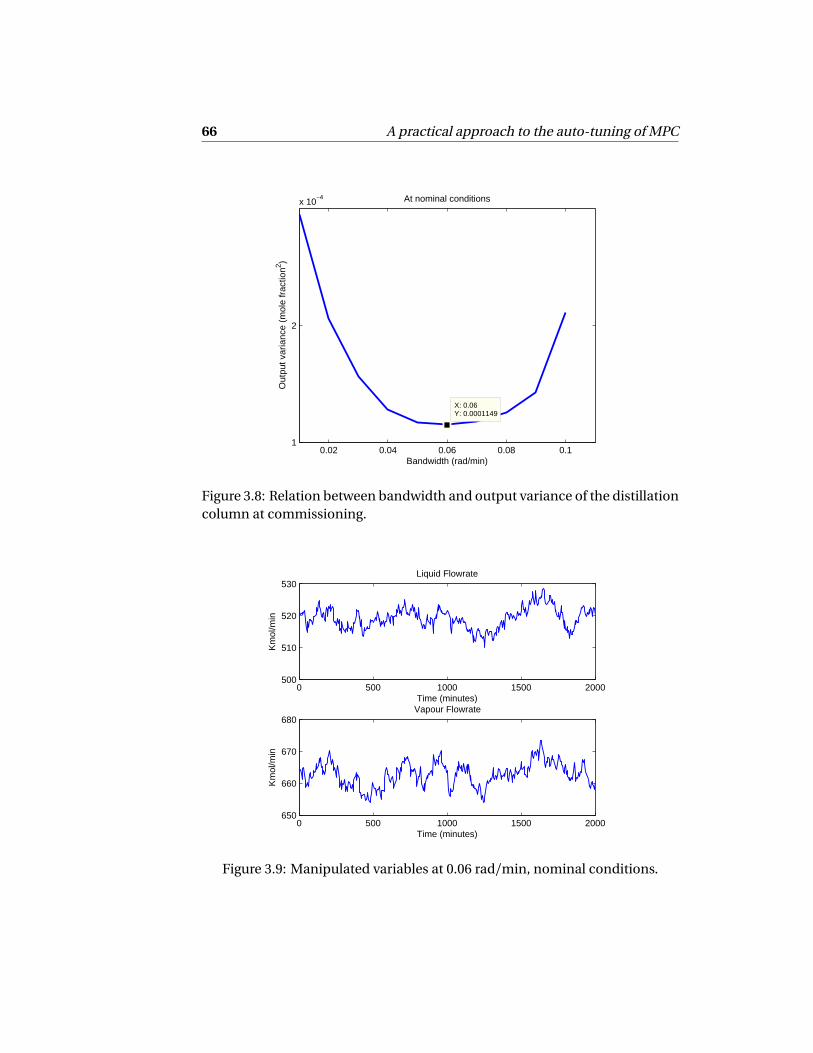
66 A practical approach to the auto-tuning of MPC
0.02 0.04 0.06 0.08 0.11
2
x 10−4
X: 0.06Y: 0.0001149
At nominal conditions
Bandwidth (rad/min)
Out
put v
aria
nce
(mol
e fr
actio
n2 )
Figure 3.8: Relation between bandwidth and output variance of the distillationcolumn at commissioning.
0 500 1000 1500 2000500
510
520
530Liquid Flowrate
Time (minutes)
Km
ol/m
in
0 500 1000 1500 2000650
660
670
680Vapour Flowrate
Time (minutes)
Km
ol/m
in
Figure 3.9: Manipulated variables at 0.06 rad/min, nominal conditions.

3.5. Implementation on a binary distillation column example 67
0 200 400 600 800 1000 1200 1400 1600 1800 20000.9
0.92
0.94
0.96
0.98Top composition
Time (minutes)
Mol
e fr
actio
n
0 200 400 600 800 1000 1200 1400 1600 1800 20000
0.02
0.04
0.06
0.08
0.1Bottom composition
Time (minutes)
Mol
e fr
actio
n
OutputsSet−points
Figure 3.10: Controlled variables at 0.06 rad/min, at nominal conditions.
rotation angle α of the model is set at −π/5. The result after re-tuning is givenin Figure 3.11. The new optimum bandwidth of 0.04 rad/min is lower thanthe commissioned one of 0.06 rad/min. It can be seen that at the commis-sioned frequency of 0.06 rad/min, the output variance goes up from 0.0001149to 0.0001757 and the auto-tuning method gives a new optimum bandwidth of0.04 rad/min at which the output variance is 0.0001595. The correspondinginput and output signals are given in Figure 3.12 and Figure 3.13, respectively.
In the third scenario, the standard deviation of the disturbance is increasedto 15 [kmol/min] for the feed rate and 0.07 [mole fraction] for the feed compo-sition, and the cut-off frequency of the filtered white noise is increased toπ/50rad/min. The result of the auto-tuning method is given in Figure 3.14. It can beseen that at the commissioned frequency of 0.06 rad/min, the output variancegoes up from 0.0001149 to 0.0002957 and the auto-tuning method gives a newoptimum bandwidth of 0.09 rad/min. At this bandwidth, the output varianceis 0.0002164. The corresponding input and output signals are given in Figure3.15 and Figure 3.16, respectively.
The results from the scenarios show how the optimum balance shifts invarious contexts. When the modelling errors become significant, the optimummoves to the left (i.e. lower bandwidth), since more robust control is required.When the disturbance becomes higher in amplitude and frequency withoutsignificantly affecting the dynamics of the plant, the optimum moves to the

68 A practical approach to the auto-tuning of MPC
0.02 0.04 0.06 0.08 0.10
1
2
3
4
5
6x 10
−4
X: 0.04Y: 0.0001595
Bandwidth (rad/min)
Out
put v
aria
nce
(mol
e fr
actio
n2 )
X: 0.06Y: 0.0001757
X: 0.06Y: 0.0001149
At commissioningAfter a plant change
Figure 3.11: Relation between bandwidth and output variance of the distilla-tion column with high modelling errors.
0 500 1000 1500 2000510
515
520
525
530Liquid Flowrate
Time (minutes)
Km
ol/m
in
0 500 1000 1500 2000655
660
665
670Vapour Flowrate
Time (minutes)
Km
ol/m
in
Figure 3.12: Manipulated variables at 0.04 rad/min, in the presence of highmodel-plant mismatch.
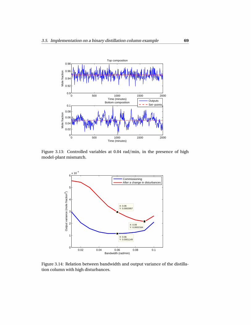
3.5. Implementation on a binary distillation column example 69
0 500 1000 1500 20000.9
0.92
0.94
0.96
0.98Top composition
Time (minutes)
Mol
e fr
actio
n
0 500 1000 1500 20000
0.02
0.04
0.06
0.08
0.1Bottom composition
Time (minutes)
Mol
e fr
actio
n
OutputsSet−points
Figure 3.13: Controlled variables at 0.04 rad/min, in the presence of highmodel-plant mismatch.
0.02 0.04 0.06 0.08 0.10
1
2
3
4
5
6x 10
−4
X: 0.09Y: 0.0002164
Bandwidth (rad/min)
Out
put v
aria
nce
(mol
e fr
actio
n2 )
X: 0.06Y: 0.0001149
X: 0.06Y: 0.0002957
CommissioningAfter a change in disturbances
Figure 3.14: Relation between bandwidth and output variance of the distilla-tion column with high disturbances.

70 A practical approach to the auto-tuning of MPC
0 500 1000 1500 2000480
500
520
540
560Liquid Flowrate
Time (minutes)
Km
ol/m
in
0 500 1000 1500 2000600
650
700
750Vapour Flowrate
Time (minutes)
Km
ol/m
in
Figure 3.15: Manipulated variables at 0.09 rad/min with high disturbances.
0 500 1000 1500 20000.9
0.92
0.94
0.96
0.98
1Top composition
Time (minutes)
Mol
e fr
actio
n
0 500 1000 1500 20000
0.02
0.04
0.06
0.08
0.1Bottom composition
Time (minutes)
Mol
e fr
actio
n
OutputsSet−points
Figure 3.16: Controlled variables at 0.09 rad/min with high disturbances.

3.5. Implementation on a binary distillation column example 71
right (i.e. larger bandwidth is required) since more control action is needed toreject the disturbances.
Due to the fact that the optimum bandwidth can vary in different condi-tions, the performance should be monitored with a varying tuning in order tokeep the system operating at its optimum bandwidth at all times. This allowsthe right control action to be taken when the current bandwidth moves awayfrom the optimum point. This is the motivation for developing the auto-tuningmethod based on extremum seeking.
3.5.5 Extremum seeking
In this subsection, the auto-tuning method based on extremum seeking in Fig-ure 3.3 is implemented on the distillation column. The auto-tuning method isapplied at nominal conditions with two different starting closed-loop band-widths: 0.02 rad/min and 0.08 rad/min. The extremum seeking runs in the toplayer of the auto-tuning to find the optimum closed-loop bandwidth and op-timisation problem (3.22) is solved to find the weighting factors in the bottomlayer while the column is in closed loop.
In these simulations, the dither signal is a sine wave of amplitude a = 0.005,the low-pass filter is enabled whereas the high-pass filter is disabled, since thisresults in halving the transient duration as discussed in Subsection 3.3.2. Fig-ures 3.17 and 3.18 show the results of the movement of the closed-loop band-width over time in the auto-tuning method at the nominal conditions. Fig-ure 3.17 shows the convergence of the closed-loop bandwidth forωe s = 0.0001[rad/min], while Figure 3.18 shows the results forωe s = 0.0002 [rad/min] withdifferent values of the integrator gain γ. The x-axis is the time of the simula-tion and the y-axis is the closed-loop bandwidth. The convergence is subjectto noise due to the stochastic properties of the disturbances and noise.
Both Figures 3.17 and 3.18 show that increasing γ results in faster conver-gence, but the estimate of the extremumω∗mp c becomes more noisy. The solidline in Figure 3.17 shows that starting from ωmp c = 0.02 [rad/min] with γ =0.0002, there appears a significant overshoot in the adaptation loop. However,starting at ωmp c = 0.08 [rad/min], under the same conditions, does not pro-duce that overshoot. This stems from the fact that the second derivative isdifferent for two different starting points. This behaviour is a known weak-ness of the classic extremum seeking algorithm. In Moase et al. (2010), the ex-tremum seeking scheme is complemented with a compensator that adapts γand a , based on local estimates of the second derivative. This modificationmight increase both the speed of convergence and stability of the extremum

72 A practical approach to the auto-tuning of MPC
seeking scheme used in this thesis, but this is still under investigation.
0 5 10 15 20 25 30 35 40 450.02
0.03
0.04
0.05
0.06
0.07
0.08
0.09
0.1
time [months]
ωm
pc [r
ad/m
in]
γ = 2e−05γ = 0.0001γ = 0.0002
Figure 3.17: Simulation results of MPC tuning in nominal conditions. ωe s =0.0001, starting points: ωmp c = 0.02 and ωmp c = 0.08.
0 5 10 15 20 25 30 35 40 450.02
0.03
0.04
0.05
0.06
0.07
0.08
0.09
0.1
time [months]
ωm
pc [r
ad/m
in]
γ = 2e−05γ = 0.0001γ = 0.0002
Figure 3.18: Simulation results of MPC tuning in nominal conditions. ωe s =0.0002, starting points: ωmp c = 0.02 and ωmp c = 0.08.
The second scenario considers a change in the plant dynamics that ap-pears 16 months after the extremum seeking method has brought the opti-mum bandwidth close to the initial optimum of 0.06 rad/min. This changeis the same as in the case of manual seeking. Figure 3.19 shows that the auto-tuning method can bring the closed-loop bandwidth close to its new optimumof about 0.04 rad/min.
The third scenario considers a change in the disturbances, instead of thechange in the plant dynamics, which occurs at the same moment. This changeis the same as in the case of manual seeking. Figure 3.20 shows that the auto-

3.6. Conclusion 73
0 10 20 30 40 500.02
0.025
0.03
0.035
0.04
0.045
0.05
0.055
0.06
0.065
0.07
Time (months)
Clo
sed−
loop
ban
dwid
th (
rad/
min
)
Plant change
Figure 3.19: Closed-loop bandwidth of the system using extremum seekingauto-tuning method. Plant change occurs at month 16.
tuning method can bring the closed-loop bandwidth close to its new optimumof about 0.085 rad/min.
3.6 Conclusion
A two-layer auto-tuning method for MPC is developed in order to find the op-timum closed-loop bandwidth and the best weighting matrices of the system.This optimum corresponds to the best trade-off between disturbance rejec-tion and robustness. The top layer uses manual or extremum seeking to findthe optimum closed-loop bandwidth. The manual seeking starts the tuningat a low closed-loop bandwidth that ensures robustness, then step-by-step in-creases this closed-loop bandwidth while monitoring the output variance untilthe optimum one is found. The extremum seeking, a model-free optimisationtechnique, finds the optimum closed-loop bandwidth in an autonomous way.It can also find the new optimum if the optimum drifts away from the previousone due to changes in plant dynamics or disturbance characteristics. The bot-tom layer addresses the connection between the closed-loop bandwidth andthe time-domain tuning parameters of MPC. The manual seeking method canfind the optimum bandwidth at different conditions, while the extremum seek-

74 A practical approach to the auto-tuning of MPC
0 10 20 30 40 50 600.02
0.03
0.04
0.05
0.06
0.07
0.08
0.09
Time (months)
Clo
sed−
loop
ban
dwid
th (
rad/
min
)
Disturbance change
Figure 3.20: Closed-loop bandwidth of the system using extremum seekingauto-tuning method. Disturbance change occurs at month 16.
ing algorithm enables the system to track its optimum closed-loop bandwidthunder various conditions. The auto-tuning method is tested on a binary distil-lation column benchmark problem. The implementation of the manual seek-ing method on an actual industrial process is described in Chapter 7.
In the top layer, the manual seeking method is an engineering approachthat is developed based on the knowledge of the plant dynamics. While it canbe used at commissioning to find the optimum, it is not very convenient to usewhen dealing with a varying optimum due to changes in plant dynamics or dis-turbance characteristics. On the other hand, the extremum seeking method issuitable in those situations. However, the main issues of extremum seekingare speed of convergence and stability. The dynamics of the distillation col-umn limit the speed at which the extremum seeking algorithm converges. Theselection of extremum seeking parameters also affects the convergence of thealgorithm. In the future, the use of a Newton-like adaptation law in the clas-sic extremum seeking scheme based on Moase et al. (2010) can be consideredin choosing the parameters of the extremum seeking algorithm. Other filterdesigns might also result in better performance. Further research could lookinto the benefits of using a high-pass filter although the analysis in Subsection3.3.2 suggests that the high-pass filter is the least critical component. In addi-

3.6. Conclusion 75
tion, reducing the duration of the filter transients could improve the speed ofconvergence. The use of a square-wave dither signal instead of a sine wave canalso be investigated. The simulation results also show that the convergence ofthe algorithm to the new optimum when there is a change in the plant or dis-turbances is much faster than the convergence to the initial optimum. Hence,in future application, the manual seeking method can be used to find the rangein which the optimum bandwidth lies, and the extremum seeking can be im-plemented in this range. This will save time for convergence and still take ad-vantage of the extremum seeking method.
The bottom layer of the auto-tuning is based on an optimisation problemin which the bandwidth of the sensitivity function is matched with the time-domain tuning parameters using an optimisation tool. This is feasible sincethe mapping between the closed-loop bandwidth and the penalty on inputsis monotonic. This can be considered as a simple "loop-shaping" based onoptimisation. For the moment, only one crossover frequency of the sensitiv-ity function is considered in the optimisation method. If more elements inthe frequency-domain sensitivity function (e.g. its slope) are considered, morecomplex weighting matrices will be required for the matching. However, suchmatching will become a complicated optimisation problem, due to the non-linear mapping from the weighting matrices to the sensitivity function. There-fore, in the following chapters, tuning methods based on controller matchingthat can be formulated as a convex optimisation problem are investigated.
The presence of constraints will limit the attainable bandwidth of the con-troller while an optimum closed-loop bandwidth still exists. For instance, whenan input saturates, one degree of freedom is dropped from the controller butthe relation between the closed-loop bandwidth and output variance still holdsfor the other degrees of freedom. This could also be verified in future work.

76 A practical approach to the auto-tuning of MPC

4A reverse-engineering tuning method
4.1 Introduction4.2 Tuning based on controller
matching
4.3 Examples4.4 Conclusion
4.1 Introduction
Chapter 3 presents a practical tuning approach in the bottom layer of the auto-tuning method of MPC. In that approach, the penalty on the input energy is cal-culated in such a way that a desired closed-loop bandwidth, which is a prac-tical controller tuning criterion, is achieved. To this end, a search method isused since the mapping from the closed-loop bandwidth to the input weightsis monotonic. The fact that only one tuning parameter is considered impliesthat the remaining degrees of freedom in the tuning have not been exploited.Intuitively, more complex cost functions with full weighting matrices will en-able us to shape the sensitivity functions more freely. However, such shapingcan lead to a complicated optimisation problem which is difficult to solve.
An alternative tuning criterion could be to make the MPC match a lineartime invariant (LTI) controller when the constraints are inactive. When theLTI controller (favourite controller) is designed based on frequency-domaintechniques such as H∞ control, the matching allows the MPC to inherit thefrequency-domain characteristics of the LTI controller. The matching of MPCwith an LTI controller when MPC is formulated using state-space representa-tion has been investigated by several authors (Rowe and Maciejowski (2000a),

78 A reverse-engineering tuning method
Cairano and Bemporad (2010) and Hartley and Maciejowski (2011, 2013)). Inthese studies, the unconstrained solution of MPC is written as a state feed-back control law and the aim of the matching is to minimise the error betweenthe state feedback gain of the favourite controller and that of MPC. The foun-dation of this approach is the inverse problem of linear optimal control, laidby Kalman (1964) and Anderson and Moore (1971). The inverse optimalityproblem is extended to a more general cost function in Kreindler and Jame-son (1972) with a cross-product term between the states and the control input.In Cairano and Bemporad (2010), a matching method based on formulating anoptimisation problem with linear matrix inequality (LMI) or bilinear matrix in-equality (BMI) constraints is proposed. The cost function of the optimisationproblem is the error between the control action of the MPC and the favouritecontroller. The matching methods based on the inverse problem of linear op-timal control usually consider the case in which the MPC is equivalent to alinear-quadratic regulator (LQR) and the states of the system are available ordetectable. In addition, in Rowe and Maciejowski (2000b), the specific match-ing to an H∞ controller designed by McFarlane and Glover (1992) is presented.
In this chapter, we present a reverse engineering tuning method which isbased on the works done by Cairano and Bemporad (2010) and Hartley andMaciejowski (2011). The method allows the MPC to behave like an H∞ con-troller given in the transfer function formulation. Using the observer-basedrealisation as shown in Alazard and Apkarian (1999), the static state feedbackgain of the favourite controller is extracted from the output feedback controller.This is followed by finding the weighting matrices of the cost function to matchthe favourite static state feedback gain. The case of a control horizon shorterthan the prediction horizon is considered. The matching with a two-degree-of-freedom H∞ controller with feed-forward control action designed based onPrempain and Postlethwaite (2001) is also investigated. The tuning of the MPCthen becomes the tuning of the weighting filters of the H∞ controller, whichgive more insight in the frequency-domain characteristics of the closed-loopsystem. In the auto-tuning method described in Section 3.3 of Chapter 3, thisreverse-engineering tuning method can therefore give a robust initial tuningbased on available information on the model-plant mismatch. In the manualseeking, the closed-loop bandwidth is then increased by changing the weight-ing filters of the H∞ controller until the optimum bandwidth is found.
In the following, the matching of MPC to one-degree-of-freedom and two-degree-of-freedom favourite controllers is presented, respectively. The match-ing with the one-degree-of-freedom controller is used to find the optimumclosed-loop bandwidth and is illustrated on the distillation column benchmarkproblem. The matching with the two-degree-of-freedom controller is illus-

4.2. Tuning based on controller matching 79
trated with a linear system, assuming that the states of the system are measur-able. Based on the results obtained with the methods discussed, conclusionsare given at the end of the chapter.
4.2 Tuning based on controller matching
This section provides preliminaries of MPC formulated in state space form withmeasured disturbances. It is shown that in the unconstrained case, MPC canbe written as a static state feedback control law combined with a static feed-forward control gain. This allows the matching of MPC to an LTI favourite con-troller. Subsection 4.2.2 then presents the reverse-engineering tuning methodbased on Hartley and Maciejowski (2011) in the case of a control horizon shorterthan the prediction horizon. The method is used to match a one-degree-of-freedom H∞ controller and the bandwidth of the H∞ controller is tuned tofind the optimum closed-loop bandwidth. Subsection 4.2.3 then introducesthe matching of MPC to a full-information two-degree-of-freedom controllerunder the assumption that all states of the system are measurable. The case ofunmeasurable states requires the observer-based realisation of feed-forwardcontrollers and is deferred for future research.
4.2.1 State-space model predictive control
Consider an LTI system given in the state-space formulation:
x (k +1) = Ax (k ) +B1d (k ) +B2u (k )y (k ) =C x (k ) +D1d (k ) +D2u (k )
(4.1)
where x (k ) is the states, u (k ) is the vector of manipulated variables, d (k ) repre-sents the measured disturbances and y (k ) is the vector of controlled outputs ofthe system. The system is often strictly proper and therefore D2 is assumed tobe 0. Assume that the reference signals of the controlled outputs are incorpo-rated in d (k ) and the control objective is to steer the outputs y (k ) to zero. Thestate-space model is used to build a prediction model as follows (Maciejowski(2002)):

80 A reverse-engineering tuning method
x (k )x (k +1)
...x (k +Hp −1)
=
IA...
AHp−1
x (k ) +
0 · · · · · · · · · 0
B2...
......
......
......
......
......
AHp−2B2 · · · · · · B2 0
u (k )u (k +1)
...u (k +Hp −1)
+
0 · · · · · · · · · 0
B1...
......
......
......
......
......
AHp−2B1 · · · · · · B1 0
d (k )d (k +1)
...d (k +Hp −1)
where Hp is the prediction horizon. Usually a control horizon Hu < Hp is se-lected, in which case u (k + l ) = u (k +Hu − 1) for l ≥ Hu and the future input
vector becomes
u (k )u (k +1)
...u (k +Hu −1)
. If no extrapolation technique is used for
predicting the measured disturbance d (k ), the prediction d (k + l ) = d (k ) forl ≥ 1 is often used. Therefore, the prediction model is given by
x (k )x (k +1)
...x (k +Hp −1)
=
IA...
AHp−1
x (k )
+
0 · · · · · · · · · 0
B2...
......
......
......
......
......
AHp−2B2 · · · · · · B2 0
I 0 · · · 0
0...
......
......
... 00 · · · 0 I0 · · · 0 I...
......
0 · · · 0 I
u (k )u (k +1)
...u (k +Hu −1)

4.2. Tuning based on controller matching 81
+
0 · · · · · · · · · 0
B1...
......
......
......
......
......
AHp−2B1 · · · · · · B1 0
II...I
d (k )
⇔ X (k ) =Ψx (k ) +ΥU (k ) +Ξd (k ) (4.2)
where X (k ) is the future state vector, U (k ) is the future input vector, and Ψ, Υand Ξ are the prediction matrices.
At each time instant k , MPC solves an optimisation problem to find theinput sequence U (k ) that minimizes a cost function:
J (k ) =Hp−1∑
i=0
x>(k + i )Qi x (k + i )
+Hu−1∑
i=0
u>(k + i −1)Ri u (k + i −1) +2u>(k + i −1)S>i x (k + i −1)
= X >(k )
Q0 0 · · · 0
0 Q1...
......
...... 0
0 · · · 0 QHp−1
︸ ︷︷ ︸
Q
X (k ) +U >(k )
R0 0 · · · 0
0 R1...
......
...... 0
0 · · · 0 RHp−1
︸ ︷︷ ︸
R
U (k )
+2U >(k )
S>0 0 · · · 0
0 S>1...
......
...... 0
0 · · · 0 S>Hu−1
x (k )x (k +1)
...x (k +Hu −1)
= X >(k )Q X (k ) +U >(k )RU (k )
+2U >(k )
>
S>0 0 · · · 0
0 S>1...
......
...... 0
0 · · · 0 S>Hu−1
I 0 · · · 0 0 · · · 0
0...
......
......
......
... 0 0 · · · 00 · · · 0 I 0 · · · 0
︸ ︷︷ ︸
S
X (k )
= X >(k )Q X (k ) +U >(k )RU (k ) +2U >(k )S>X (k )
= (Ψx (k ) +ΥU (k ) +Ξd (k ))>Q (Ψx (k ) +ΥU (k ) +Ξd (k )) +U >(k )RU (k )
+2U >(k )S> (Ψx (k ) +ΥU (k ) +Ξd (k )) . (4.3)

82 A reverse-engineering tuning method
The solution to the corresponding unconstrained optimisation problem isgiven by
U (k ) =−
Υ>QΥ +R +2S>Υ−1 Υ>QΨ +S>Ψ
x (k )
−
Υ>QΥ +R +2S>Υ−1 Υ>QΞ+S>Ξ
d (k ) (4.4)
Since only the first element of the input sequence is implemented, the actualcontrol input at time k is
u (k ) =−Θ
Υ>QΥ +R +2S>Υ−1 Υ>QΨ +S>Ψ
x (k )
−Θ
Υ>QΥ +R +2S>Υ−1 Υ>QΞ+S>Ξ
d (k )
= K x (k ) + Ld (k ) (4.5)
where Θ =
I 0 · · · 0
. This shows that the unconstrained MPC can bewritten as a static control law, where K represents the feedback part and L rep-resents the feed-forward part. This is the basis for matching MPC to a givenfavourite LTI control law. In the following, the matching of MPC with one-degree-of-freedom and two-degree-of-freedom favourite controllers is shown.
4.2.2 Matching to a one-degree-of-freedom favourite controller
In this subsection, the matching of MPC to a one-degree-of-freedom H∞ con-troller is presented. Note that in this case, no measured disturbances are con-sidered and control action (4.5) reduces to u (k ) = K x (k ). The one-degree-of-freedom H∞ controller is designed according to the scheme given in Figure4.1. In Figure 4.1, Wu is the input weighting filter and We is the output errorweighting filter, di is the unmeasured input disturbance and d y is the unmea-sured output disturbance. The detailed guidelines for choosing the weightingfilters for process applications can be found in Lundström et al. (1991a,b). Wu
represents the input uncertainty weight and is chosen as a high-pass filter sincethe modelling errors usually tend to be significant at high frequencies. We is theperformance weight and chosen as a low-pass filter which decides the level ofdisturbance rejection of the system. ∆ represents any transfer function thatsatisfies ‖∆‖∞ ≤ 1. The H∞ problem is to find a controller K (z ) such that the∞-norm of the transfer matrix from the exogenous inputs di , d y and r to thecontrolled outputs e1 and e2 is smaller than a performance criterion γ. Thisproblem is solved using the LMI-based parameterisation described in Gahinetand Apkarian (1993). Assume that the state-space formulation of the H∞ con-troller is given by:

4.2. Tuning based on controller matching 83
xK (k +1) = AK xK (k ) +BK y (k )u (k ) =CK xK (k ) +DK y (k )
(4.6)
and that the number of states of the controller nK is equal to the number ofstates of the plant n . According to Alazard and Apkarian (1999) and Hartley andMaciejowski (2011), the closed-loop system can be written in the compensator-observer form as follows:
x (k +1|k ) = Ax (k |k −1) +B u (k ) +K f
y (k )−C x (k |k −1)
u (k ) = Kc x (k |k −1) +DQ
y (k )−C x (k |k −1) (4.7)
where x is the states of the closed-loop system, K f and Kc are the observergain and state feedback gain and DQ is the feed-through from the measuredoutput y (k ) to the control input u (k ). The computation of K f , Kc and DQ isbased on solving the following Riccati equation (Alazard and Apkarian (1999)and Hartley and Maciejowski (2011)) with the variable T :
−T I
A+B DK C B CK
BK C AK
IT
= 0 (4.8)
K f , Kc and DQ are then given by
K f = T −1BK −B DK
Kc =−CK T −DK C
DQ =DK
(4.9)
Detailed proof of the result is found in Alazard and Apkarian (1999). Note thatthe Riccati equation (4.8) generally has finitely many solutions T . The closed-
loop system matrix
A+B DK C B CK
BK C AK
has 2n eigenvalues and each partic-
ular choice of n eigenvalues corresponds to one solution T . Therefore, thereare finitely many choices of K f , Kc and DQ for one output-feedback favouritecontroller.
MPC control action (4.5) shows no feed-through from measured outputsto control inputs. Therefore, the term DQ in (4.7) prevents the matching frombeing feasible. Since DQ =DK (Alazard and Apkarian (1999)), a strictly properfavourite controller with DK = 0 will lead to DQ = 0 and the matching of Kc

84 A reverse-engineering tuning method
K(z) P(z)∑
-u(k)
We(z)
Wu(z)
r(k) + Ɛ(k)
e1(k)
e2(k)
∑
Δ
∑
dy(k)
di(k)
y(k)
Figure 4.1: Scheme of an H∞ controller.
and K will result in an MPC behaving like the favourite controller. There areseveral ways of making DK = 0. In this work, a loop-shifting technique (Hartleyand Maciejowski (2011)) is used. Assume y (k ) =C x (k ), the state-space formu-lation of the controller is given by:
xK (k +1) = AK xK (k ) +BK y (k )u (k ) =CK xK (k ) +DK C x (k )
. (4.10)
Let u2(k ) = u (k )−DK C x (k ) and the state-space formulation of the open-loopsystem is:
x (k +1) = Ax (k ) +B u (k ) = (A+B DK C )x (k ) +B u2(k )y (k ) =C x (k )
. (4.11)
Therefore, if u2(k ) is considered as the control input of the system, the term DK
has been "shifted" to the dynamics of the plant and removed from the dynam-ics of the controller. Let Ane w = A+B DK C , the compensator-observer form ofthe controller is then given by:
x (k +1|k ) = Ane w x (k |k −1) +B u (k ) +K f
y (k )−C x (k |k −1)
u2(k ) = Kc x (k |k −1)(4.12)
which allows the matching to be performed by finding the MPC tuning param-eters such that K = Kc , namely finding Q , R and S such that:

4.2. Tuning based on controller matching 85
Kc =−Θ
Υ>QΥ +R +2S>Υ−1 Υ>QΨ +S>Ψ
(4.13)
The non-invertibility of Θ is the major problem of this matching, since itmakes it impossible to reformulate the optimisation problem:
minQ ,R ,S
‖Kc −K ‖ (4.14)
subject to
Q SS> R
> 0 as a convex optimisation problem with LMI con-
straints unless Hu = 1. In order to overcome this, the favourite feedback gainof the whole input sequence needs to be assigned, not only the first elementKc . The matching problem then becomes:
Kc
Kc1...
KcHu−1
=−
Υ>QΥ +R +2S>Υ−1 Υ>QΨ +S>Ψ
(4.15)
where Kc1, . . . , KcHu−1
are determined such that the future inputs also match thefavourite controller, namely:
u (k +1) = Kc x (k +1) = Kc (A+B Kc )x (k )u (k +2) = Kc x (k +2) = Kc (A+B Kc )
2 x (k )...
u (k +Hu −1) = Kc x (k +Hu −1) = Kc (A+B Kc )Hu−1 x (k ).
(4.16)
Therefore:
Kc1
Kc2...
KcHu−1
=
Kc (A+B Kc )Kc (A+B Kc )
2
...Kc (A+B Kc )
Hu−1
(4.17)
and the matching problem can be written as a convex optimisation problemwith LMI constraints:

86 A reverse-engineering tuning method
minQ ,R ,S
Υ>QΥ +R +2S>Υ
Kc
Kc1...
KcHu−1
+
Υ>QΨ +S>Ψ
(4.18)
subject to
Q SS> R
> 0.
Optimisation problem (4.18) shows that the longer the control horizon Hu ,the more complex the optimisation and the more likely to be significant theerror. Hence, with long control horizon, more elements in the weighting ma-tricesQ , R and S should be included in the optimisation to increase the degreesof freedom. Solving this optimisation problem provides the weighting matri-ces that make the MPC behave like the favourite controller when constraintsare inactive. Matching the MPC to an H∞ controller translates the tuning ofthe time-domain parameters into the tuning of the weighting filters of the H∞controller.
For example, this matching method can be used in the manual seekingtwo-layer auto-tuning method described in Subsection 3.3.1 of Chapter 3. Theauto-tuning method then consists of the following steps:
1. Initialisation: Design a favourite H∞ controller: Determine and fix theuncertainty weight (input weight) based on initial knowledge of model-plant mismatch. Design a low-bandwidth performance weight (outputweight) with low-frequency and high-frequency gains satisfying specifi-cations of the system. Find the corresponding MPC tuning parametersby the reverse-engineering method. The control horizon and the predic-tion horizon are fixed based on the engineering rules given in Chapter 1.The output variance for this initial tuning is then calculated.
2. Seeking: Increase the bandwidth of the performance weight while mon-itoring the output variance. Find the corresponding MPC tuning param-eters by the reverse-engineering tuning method.
3. Monitoring: Monitor the output variance. Compare it with the previoustuning. If the variance decreases, keep raising the bandwidth. If it in-creases, the previous tuning is optimum.

4.2. Tuning based on controller matching 87
4.2.3 Matching to a two-degree-of-freedom favourite controller
The performance of MPC strongly relies on the quality of the prediction model.Therefore, it is natural that almost any signal that is measurable but not used asan MV or CV will be used as a measured disturbance, or a feed-forward signalin the prediction model. In other words, the prediction model of MPC usuallymakes use of all the information available at the moment it is made. Hence,the feed-forward part of the MPC should also be included in the reverse en-gineering tuning method. In this case, the favourite controller is designed toguarantee certain characteristics in the transfer function from the measureddisturbances to the CV’s. Such a favourite controller is called a two-degree-of-freedom controller. This section introduces a method of matching MPC to atwo-degree-of-freedom LTI controller. The design of the favourite controller isbased on Prempain and Postlethwaite (2001), where the design problem is re-cast as a full-information synthesis using LMI. The design of the favourite con-troller is first introduced, followed by finding the weighting matrices of MPCfor the matching.
With the assumption that the states of the system are measurable, the com-putation of the control law of the favourite controller is formulated as an LMIproblem. The scheme of a full-information two-degree-of-freedom controlleris given in Figure 4.2. In this figure, Wr (z ) is a transfer function used to filter thereference signal r1(k ) and d (k ) represents any measured disturbances enteringthe system P (z ).
Assume that the system P (z ) is represented by the following state-spaceformulation:
x (k +1) = Ax (k ) +B1d (k ) +B2 (u (k ) +di (k ))y (k ) =C x (k ) +D1d (k ) +D2 (u (k ) +di (k ))+d y (k )
(4.19)
Wr is represented by:
xr (k +1) = Ar xr (k ) +Br r1(k )r (k ) =Cr xr (k ) +Dr r1(k )
(4.20)
Wp is represented by:
xe (k +1) = Ae xe (k ) +Be
r (k )− y (k )
e1(k ) =Ce xe (k ) +De
r (k )− y (k ) (4.21)
and Wu is represented by:

88 A reverse-engineering tuning method
P(z)∑ u(k)Wr(z)
Wu(z)
e1(k)
e2(k)
∑
Δ
∑
dy(k)
di(k)
y(k)r1(k)
We(z)
d(k)
x(k)
d(k)
r(k)
r(k)
-+
K(z)
Figure 4.2: Scheme of a full-information two-degree-of-freedom H∞ con-troller.
xu (k +1) = Au xu (k ) +Bu u (k )e2(k ) =Cu xu (k ) +Du u (k )
. (4.22)
The augmented plant is then given by the representation:
xa ug (k +1) = Aa ug xa ug (k ) +B1a ug da ug (k ) +B2a ug u (k )ya ug (k ) =Ca ug xa ug (k ) +D1a ug da ug (k ) +D2a ug u (k )
(4.23)
where xa ug (k ) =
x (k )xr (k )xe (k )xu (k )
, da ug (k ) =
d (k )r1(k )d y (k )di (k )
and ya ug (k ) =
e1(k )e2(k )
. The
augmented system matrices are:

4.2. Tuning based on controller matching 89
Aa ug =
A 0 0 00 Ar 0 0
−Be C Be Cr Ae 00 0 0 Au
;B1a ug =
B1 0 0 B2
0 Br 0 0−Be D1 Be Dr −Be −Be D2
0 0 0 0
;
B2a ug =
B2
0−Be D2
Bu
and
Ca ug =
−De C De Cr Cp 00 0 0 Cu
; D1a ug =
−De D1 De Dr −De −De D2
0 0 0 0
;
D2a ug =
−De D2
Du
.
The aim of the design is to find the full-information control law:
u (k ) = F1 xa ug (k ) + F2
d (k )r1(k )
= F1 xa ug (k ) +
F2 0
da ug (k )
= F1 xa ug (k ) + F2da ug (k ) (4.24)
such that the H∞-norm of the closed-loop system from da ug (k ) to ya ug (k ) islower than a performance criterion γ. With this control law, the closed-loopsystem from da ug (k ) to ya ug (k ) is given by:
xa ug (k +1) =
Aa ug +B2a ug F1
xa ug (k ) +
B1a ug +B2a ug F2
da ug (k )ya ug (k ) =
Ca ug +D2a ug F1
xa ug (k ) +
D1a ug +D2a ug F2
da ug (k ).
(4.25)
According to the Bounded Real Lemma (Gahinet and Apkarian (1993)), thereexists a control law u (k ) = F1 xa ug (k ) + F2da ug (k ) such that the H∞-norm ofthe closed-loop system from da ug (k ) to ya ug (k ) is lower than a performancecriterion γ if and only if there exist X = X > > 0 and F2 that satisfy:

90 A reverse-engineering tuning method
−X Aa ug +B2a ug F1 B1a ug +B2a ug F2 0
Aa ug +B2a ug F1
> −X −1 0
Ca ug +D2a ug F1
>
B1a ug +B2a ug F2
>0 −γI
D1a ug +D2a ug F2
>
0 Ca ug +D2a ug F1 D1a ug +D2a ug F2 −γI
< 0
(4.26)
Left and right multiplying (4.26) with
I 0 0 00 X 0 00 0 I 00 0 0 I
gives:
−X Aa ug X +B2a ug Y B1a ug +B2a ug F2 0
Aa ug X +B2a ug Y> −X 0
Ca ug X +D2a ug Y>
B1a ug +B2a ug F2
>0 −γI
D1a ug +D2a ug F2
>
0 Ca ug X +D2a ug Y D1a ug +D2a ug F2 −γI
< 0
(4.27)
where Y = F1X . Solving LMI (4.27) provides the static H∞ control law F1 =Y X −1 and F2. Hence, the objective of the reverse-engineering tuning method isto find the weighting matrices Q , R and S such that K = F1 and L = F2. Similarlyto Subsection 4.2.2, the aim of the matching is to ensure that the whole inputsequence produces the behaviour of the favourite controller. Assume constantprediction for the measured disturbances, namely d (k ) = d (k +1) = . . .= d (k +
Hp ) and r1(k ) = r1(k + 1) = . . . = r1(k +Hp ) and let w (k ) =
d (k )r1(k )
, the future
input elements of the favourite controller are given by:
u (k +1) = F1 x (k +1) + F2w (k ) (4.28)
= F1
Aa ug +B2a ug F1
x (k ) + F1
B1a ug +B2a ug F2
w (k ) + F2w (k ) (4.29)
= F1
Aa ug +B2a ug F1
x (k ) +
F1
B1a ug +B2a ug F2
+ F2
w (k ) (4.30)
u (k +2) = F1
Aa ug +B2a ug F1
2x (k )
+
F1
Aa ug +B2a ug F1
B1a ug +B2a ug F2
+B1a ug +B2a ug F2
+ F2
w (k )(4.31)
...
u (k + i ) = F1
Aa ug +B2a ug F1
ix (k )
+
F1
i−1∑
j=0
Aa ug +B2a ug F1
j B1a ug +B2a ug F2
!
+ F2
!
w (k ). (4.32)

4.3. Examples 91
Hence, the matching problem is formulated as the following optimisation prob-lem:
min
Υ>QΥ +R +2S>Υ
F1
F11
...F1Hu−1
+
Υ>QΨ +S>Ψ
+
Υ>QΥ +R +2S>Υ
F2
F21
...F2Hu−1
+
Υ>QΞ+S>Ξ
(4.33)
subject to
Q SS> R
> 0, where
F11
F12...
F1Hu−1
=
F1
Aa ug +B2a ug F1
F1
Aa ug +B2a ug F1
2
...
F1
Aa ug +B2a ug F1
Hu−1
(4.34)
and
F2
F21...
F2Hu−1
=
F1
B1a ug +B2a ug F2
+ F2
F1
1∑
j=0
Aa ug +B2a ug F1
j B1a ug +B2a ug F
+ F2
...
F1
Hu−2∑
j=0
Aa ug +B2a ug F1
j B1a ug +B2a ug F
+ F2
. (4.35)
Solving this optimisation problem provides the weighting matrices that makethe MPC behave like the favourite controller when constraints are inactive.
4.3 Examples
In this section, two examples are considered. The first example is the binarydistillation column benchmark described in Chapter 3. An initial H∞ con-troller is designed for the column and the reverse-engineering tuning method
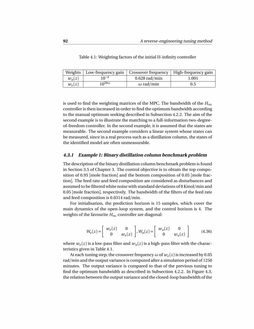
92 A reverse-engineering tuning method
Table 4.1: Weighting factors of the initial H-infinity controller
Weights Low-frequency gain Crossover frequency High-frequency gainwu (z ) 10−4 0.628 rad/min 1.001we (z ) 1020ω ω rad/min 0.5
is used to find the weighting matrices of the MPC. The bandwidth of the H∞controller is then increased in order to find the optimum bandwidth accordingto the manual optimum seeking described in Subsection 4.2.2. The aim of thesecond example is to illustrate the matching to a full-information two-degree-of-freedom controller. In the second example, it is assumed that the states aremeasurable. The second example considers a linear system whose states canbe measured, since in a real process such as a distillation column, the states ofthe identified model are often unmeasurable.
4.3.1 Example 1: Binary distillation column benchmark problem
The description of the binary distillation column benchmark problem is foundin Section 3.5 of Chapter 3. The control objective is to obtain the top compo-sition of 0.95 [mole fraction] and the bottom composition of 0.05 [mole frac-tion]. The feed rate and feed composition are considered as disturbances andassumed to be filtered white noise with standard deviations of 8 Kmol/min and0.05 [mole fraction], respectively. The bandwidth of the filters of the feed rateand feed composition is 0.0314 rad/min.
For initialisation, the prediction horizon is 15 samples, which cover themain dynamics of the open-loop system, and the control horizon is 4. Theweights of the favourite H∞ controller are diagonal:
We (z ) =
we (z ) 00 we (z )
, Wu (z ) =
wu (z ) 00 wu (z )
(4.36)
where we (z ) is a low-pass filter and wu (z ) is a high-pass filter with the charac-teristics given in Table 4.1.
At each tuning step, the crossover frequencyω of we (z ) is increased by 0.05rad/min and the output variance is computed after a simulation period of 1250minutes. The output variance is compared to that of the previous tuning tofind the optimum bandwidth as described in Subsection 4.2.2. In Figure 4.3,the relation between the output variance and the closed-loop bandwidth of the

4.3. Examples 93
0.05 0.06 0.07 0.08 0.09 0.11.35
1.36
1.37
1.38
1.39
1.4
1.41
1.42
1.43
1.44
1.45x 10
−4
X: 0.075Y: 0.0001353
Relation between closed−loop bandwidth and output variance
Closed−loop bandwidth (rad/min)
Out
put v
aria
nce
Figure 4.3: Relation between bandwidth and output variance of the distillationcolumn.
system is provided. It is shown that 0.075 rad/min is the optimum bandwidthof the system where the output variance is 0.0001353. The input and outputsignals at the optimum bandwidth of 0.075 rad/min are given in Figures 4.4and 4.5.
4.3.2 Example 2: Linear system based on the distillation column bench-mark
Consider the linear system that represents the dynamics of the distillation col-umn benchmark at the chosen operating point:
x (k +1) =
0.8179 0.0008110.03207 0.8252
x (k ) +
0.01164 −0.01188 0.007079 2.2190.002965 0.01087 −0.01729 −1.339
u (k )
y (k ) =
0.1362 −0.032440.05586 0.02369
x (k )
(4.37)
In this model, the first two inputs are the control inputs, the third input whichrepresents the feed rate is the measurable disturbance and the fourth inputwhich represents the feed composition is the non-measurable disturbance. There-

94 A reverse-engineering tuning method
0 200 400 600 800 1000 1200 1400510
520
530
540
550Liquid flowrate
Time (minutes)
Km
ol/m
in
0 200 400 600 800 1000 1200 1400650
660
670
680
690Vapour flowrate
Time (minutes)
Km
ol/m
in
Figure 4.4: Control inputs of the system at the optimum bandwidth of 0.075rad/min.
0 200 400 600 800 1000 1200 14000.9
0.92
0.94
0.96
0.98
1Top composition
Time (minutes)
Mol
e fr
actio
n
0 200 400 600 800 1000 1200 14000
0.02
0.04
0.06
0.08
0.1Bottom composition
Time (minutes)
Mol
e fr
actio
n
Figure 4.5: Controlled outputs of the system at the optimum bandwidth of0.075 rad/min (-), and their set-points (-).

4.3. Examples 95
Table 4.2: Weighting factors of the two-degree-of-freedom H-infinity controller
Weights Low-frequency gain Crossover frequency High-frequency gainwu (z ) 10−4 0.628 rad/min 1.001we (z ) 5.103 0.1 rad/min 0.5wr (z ) 1 0.05 rad/min 10−5
fore, the model from the fourth input to the outputs is only used for simulationand not used in either the MPC prediction or the design of the two-degree-of-freedom controller. The sampling time of the model is 5 minutes. A full-information two-degree-of-freedom controller is designed as shown in Subsec-tion 4.2.3. The controller uses the measurable disturbance and the referenceas feed-forward signals. The weighting filters of the controller are given by:
We (z ) =
we (z ) 00 we (z )
, Wu (z ) =
wu (z ) 00 wu (z )
andWr (z ) =
wr (z ) 00 wr (z )
.
The characteristics of the transfer functions we , wu and wr are given in Table4.2.
The static gain of the H∞ controller is
F1 =
−13.6916 −11.9412 −2.2634 13.8949 −32.4726 199.8401 3.4359 −0.20795.5180 −12.5997 −6.0473 9.9010 −87.0523 142.3380 −0.2251 3.5490
(4.38)
and
F2 =
0.1117 −16.4572 101.33300.2210 −44.1528 72.1652
(4.39)
Although there is only one measurable disturbance in the model, matrix F2
has 3 columns since the references of the outputs are also considered as mea-sured disturbances in the controller, according to the scheme in Figure 4.2. Inthis example, the prediction horizon is 15 and the control horizon is 3. Thecontrol horizon in this case is chosen shorter than the previous case becausethe matching of the feed-forward part renders the optimisation problem more

96 A reverse-engineering tuning method
0 500 1000 1500 2000 2500−5
0
5
10
15
Time (minutes)
Mea
sure
d di
stur
banc
es
0 500 1000 1500 2000 2500−0.06
−0.04
−0.02
0
0.02
Time (minutes)
Unm
easu
red
dist
urba
nces
Figure 4.6: Disturbance signals used in simulation.
complex and time-consuming. Optimisation problem (4.33) gives the weight-ing matrices Q , R and S . The optimisation problem is solved using the Sedumisolver of Yalmip (Löfberg (2004)). Let
K1 =−
Υ>QΥ +R +2S>Υ
Υ>QΨ +S>Ψ
K2 =−
Υ>QΥ +R +2S>Υ
Υ>QΞ+S>Ξ (4.40)
the error of the solution is given by:
‖K1− F1‖2 = 0.9610‖K2− F2‖2 = 0.0018.
(4.41)
In this example, a simulation of 500 samples, namely 2500 minutes is per-formed. The measured and unmeasured disturbances in the simulation aregiven in Figure 4.6.
Step changes of -0.02 for output 1 and of 0.02 for output 2 at 50 minutesare also considered. An upper limit of 538 for the first input of the system isimposed. The output and input signals of the MPC and the full-informationH∞ controller are given in Figure 4.7 and 4.8, respectively. As shown in Figure4.7 and 4.8, when the input constraints are inactive, the two controllers behave

4.4. Conclusion 97
0 500 1000 1500 2000 2500−0.05
0
0.05
0.1
0.15
Time (minutes)
0 500 1000 1500 2000 25000.94
0.96
0.98
1
1.02
Time (minutes)
Favourite controllerMPC
Figure 4.7: Outputs of the system in closed loop.
in the same way. When the input constraint is active, the MPC tries to use theother input to control the system and the matching is therefore impossible.
4.4 Conclusion
The first part of this chapter presents a reverse-engineering tuning methodbased on Hartley and Maciejowski (2011) and uses it to match a one-degree-of-freedom H∞ controller. The H∞ controller is designed in the frequencydomain and its state feedback gain and observer gain are extracted using theobserver-based realisation described in Hartley and Maciejowski (2011) andAlazard and Apkarian (1999). The observer is used in the MPC and the weight-ing matrices are computed to match the state feedback gain. The tuning ofthe MPC then becomes the tuning of the H∞ controller, which gives more in-sight in the frequency-domain characteristics of the system and can make useof the literature on H∞ weight selection (e.g. Lundström et al. (1991a,b)). Themethod is illustrated with the binary distillation column benchmark problemdescribed in Chapter 3.
The second part of this chapter presents the design of the full-informationtwo-degree-of-freedom H∞ controller and finds the MPC tuning parameters
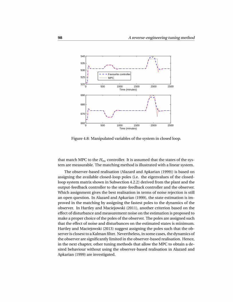
98 A reverse-engineering tuning method
0 500 1000 1500 2000 2500520
525
530
535
540
Time (minutes)
0 500 1000 1500 2000 2500660
670
680
690
Time (minutes)
Favourite controllerMPC
Figure 4.8: Manipulated variables of the system in closed loop.
that match MPC to the H∞ controller. It is assumed that the states of the sys-tem are measurable. The matching method is illustrated with a linear system.
The observer-based realisation (Alazard and Apkarian (1999)) is based onassigning the available closed-loop poles (i.e. the eigenvalues of the closed-loop system matrix shown in Subsection 4.2.2) derived from the plant and theoutput-feedback controller to the state-feedback controller and the observer.Which assignment gives the best realisation in terms of noise rejection is stillan open question. In Alazard and Apkarian (1999), the state estimation is im-proved in the matching by assigning the fastest poles to the dynamics of theobserver. In Hartley and Maciejowski (2011), another criterion based on theeffect of disturbance and measurement noise on the estimation is proposed tomake a proper choice of the poles of the observer. The poles are assigned suchthat the effect of noise and disturbances on the estimated states is minimum.Hartley and Maciejowski (2013) suggest assigning the poles such that the ob-server is closest to a Kalman filter. Nevertheless, in some cases, the dynamics ofthe observer are significantly limited in the observer-based realisation. Hence,in the next chapter, other tuning methods that allow the MPC to obtain a de-sired behaviour without using the observer-based realisation in Alazard andApkarian (1999) are investigated.

4.4. Conclusion 99
The reverse-engineering tuning methods also consider the MPC formula-tion in the state-space representation and a cost function penalising the statesand the inputs. Another popular cost function in MPC implementation pe-nalises the outputs and inputs. This is the motivation for investigating the MPCformulated in transfer functions and a cost function penalising input and out-put signals.

100 A reverse-engineering tuning method

5Generalised Predictive Control tuning by
controller matching
5.1 Introduction5.2 Preliminaries: Generalised
Predictive Control5.3 Problem formulation5.4 Matching transfer matrices
5.5 Finding the weightingmatrices
5.6 Example5.7 Conclusion and future work
5.1 Introduction
The controller matching methods presented in the previous chapter consid-ers the case in which the states of the system are available or detectable. Inmany applications, the states of the system are not measurable and the use ofa state observer is required. In Rowe and Maciejowski (2000a), the observeris designed and the tuning parameters of the MPC are found by investigatingthe inverse problem of the normalized left co-prime factorisation (NLCF) opti-mal control. In Rowe and Maciejowski (2000b), separate designs of the robustobserver and state feedback gain are used for the matching purpose, and non-convex optimisation techniques are employed to perform the matching whenthe terminal weight is not used.
In Doyle and Stein (1978), it is shown that robustness is not guaranteedeven when one attempts to design a “good" observer and a state feedback gain.

102 Generalised Predictive Control tuning by controller matching
Based on this observation, Hartley and Maciejowski (2011) makes use of the ob-server realisation techniques described in Alazard and Apkarian (1999) to de-compose a favourite controller into the observer part and state feedback partbefore performing the matching. If a favourite output feedback controller con-tains a feed-through term from the outputs to the control inputs (i.e. a non-strictly-proper controller), loop-shifting techniques must be used to “transfer"the feed-through term to the dynamics of the plant to make the matching fea-sible. By introducing some assumptions, Hartley and Maciejowski (2013) pro-pose a solution to the problem by considering the feed-through term in theframework of reference tracking.
Due to the nature of the inverse optimality problem (Kalman (1964), An-derson and Moore (1971) and Kreindler and Jameson (1972)), the controllermatching is often studied with a state-feedback MPC law and an observer de-sign. Nevertheless, MPC can also be formulated by transfer functions and thisformulation is also well adopted by several MPC providers in the process in-dustry (Clarke (1988) and Qin and Badgwell (2003)). The MPC based on trans-fer function models (GPC) was introduced in Clarke et al. (1987a,b), Clarkeand Mohtadi (1989) and further developed in Albertos and Ortega (1989) andRossiter (2005). Hence, the matching of GPC with a favourite controller is in-vestigated in this chapter, with the aim of tackling the feed-through term fromthe outputs to the inputs in a direct way. Furthermore, since not every costfunction x>(k )Qx x (k ) which penalises the states can easily be converted intoy >(k )Qy y (k )which penalises the outputs, the feasibility conditions of match-ing GPC with a favourite controller are of great interest. In the matching methodby Cairano and Bemporad (2010), the inputs and outputs are arranged as statesof the system, which help make use of state-space matching methods withoutusing a state observer. In this chapter, we also investigate the use of a filterT (z ) in GPC when performing the matching, since such a filter can be usefulin some applications. A control horizon different from the prediction horizoncan also be considered with the proposed method.
In terms of GPC tuning, Shah and Engell (2010, 2011) propose a tuningmethod for the GPC such that the poles and zeros of the closed-loop system ap-proximate certain desired ones. Shah and Engell (2013) make use of optimisa-tion techniques to find an output feedback gain that minimises the differencebetween the closed-loop behaviour of the GPC and the desired behaviour in thefrequency domain. In that work, the tuning parameters are found by solving aconvex optimisation problem with LMI constraints. The approach is limitedto the case where the control horizon is 1. As shown in Section 2.3 of Chap-ter 2, the tuning rules for the weights in GPC in literature are quite heuristic.Clarke and Mohtadi (1989) choose 0 or a small value for the input weight and

5.2. Preliminaries: Generalised Predictive Control 103
tune the auxiliary model to perform pole-placement. Yoshitani and Hasegawa(1998) use the input weight of 0.6 in their GPC for their heating furnace in con-tinuous annealing to obtain a satisfactory performance. Karacan et al. (2001)select a final value of 1.2 for the input weight after testing different values onthe simulated system. Yamamoto et al. (2003) choose the input weight basedon the small gain theorem (Zhou et al. (1996)) and therefore information on themodel uncertainty is required. Banerjee and Shah (1992) show the de-tuningeffect when the input weight is reduced and an input weight larger than 1 andsmaller than 2 is proposed to guarantee some level of robustness while ensur-ing the closed-loop nominal performance.
Since many applications of GPC use pragmatic tuning methods, an objec-tive of this chapter is to develop an analytical tuning method for GPC. The focusis to match a GPC using a quadratic cost function to a favourite controller whenthe constraints are inactive. Instead of using optimisation techniques, we solvea set of linear equations to find the output feedback gain of GPC. To this end,the rank conditions of coefficient matrices are investigated. Once the rank con-ditions are fulfilled, an output feedback gain that guarantees the matching canalways be found. Then, a convex optimisation problem with LMI constraintssimilar to that in Cairano and Bemporad (2010) is used to find the tuning pa-rameters which provide the computed output feedback gain. The degrees offreedom of the problem are increased by extending the objective function ofthe GPC with cross-product terms between the outputs and inputs. The pro-posed approach allows a control horizon larger than 1. Moreover, the matchingof the transfer functions can also be used for matching the feed-forward con-trol in the favourite controller.
This chapter is organised as follows. Section 5.2 presents the formulationand notations used throughout the chapter. Section 5.3 formulates the prob-lem and Section 5.4 provides the method to find the output feedback gain forthe matching. The approach to computing the tuning parameters is given inSection 5.5. Section 5.6 illustrates the method with the binary distillation col-umn benchmark problem described in Chapter 3 and Section 5.7 gives con-cluding comments.
5.2 Preliminaries: Generalised Predictive Control
Consider a linear system described by a Controlled auto-regressive integratedmoving average (CARIMA) model (Rossiter (2005)) with nu inputs, nd measur-able disturbances and ny outputs:

104 Generalised Predictive Control tuning by controller matching
D (z )yk =N (z )uk + F (z )dk +T (z )∆(z )
vk (5.1)
where N (z )ny×nu and D (z )ny×ny are the numerator and denominator matri-ces of the system, respectively; F (z )ny×nd is the numerator of the feed-forwardmodel from dk to yk ; T (z ) = t (z )Iny
is a diagonal transfer matrix used to modelthe disturbance signal and usually considered as a design parameter (Clarkeet al. (1987a,b)); ∆(z ) is the difference operator ∆(z ) = 1− z−1; yk ∈ Rny , uk ∈Rnu , dk ∈ Rnd and vk ∈ Rny represent the output, input, measurable distur-bance and a zero-mean random variable at time instant k , respectively.
In the rest of the chapter, a system where nu = ny = nd is considered forthe sake of simplicity, although the proposed method can be extended to thecase of non-square systems using the same procedure. However, the feasibilityconditions of the matching can change. The output reference is assumed to beincorporated in the model and the aim of the controller is to steer the outputsof the system to zero.
From (5.1), it follows:
D (z )∆(z )T −1(z )yk =N (z )T −1(z )∆uk + F (z )T −1(z )∆dk + vk (5.2)
⇒D (z )∆(z ) yk =N (z )∆uk + F (z )∆dk + vk (5.3)
where yk = T −1(z )yk , uk = T −1(z )uk and dk = T −1(z )dk are the filtered out-puts, filtered inputs and filtered disturbance signals, respectively. With the as-sumption that the considered system is strictly proper, let
D (z )∆(z ) = I +D1z−1+D2z−2+ . . . Dn+1z−n−1 (5.4)
N (z ) =N1z−1+N2z−2+ . . .+Nn z−n (5.5)
and
F (z ) = F1z−1+ F2z−2+ . . . Fn z−n . (5.6)
Let Hp denote the prediction horizon, the prediction model of the systemis constructed as follows (with the assumption that the best prediction of vk iszero):
yk+1+D1 yk + . . .+Dn+1 yk−n =
N1∆uk + . . .+Nn∆uk−n+1+ F1∆dk + . . .+ Fn∆dk−n+1
yk+2+D1 yk+1+ . . .+Dn+1 yk−n+1 =

5.2. Preliminaries: Generalised Predictive Control 105
N1∆uk+1+ . . .+Nn∆uk−n+2+ F1∆dk+1+ . . .+ Fn∆dk−n+2
...
yk+Hp+D1 yk+Hp−1+ . . .+Dn+1 yk+Hp−1−n =
N1∆uk+Hp−1+ . . .+Nn∆uk+Hp−n + F1∆dk+Hp−1+ . . .+ Fn∆dk+Hp−n . (5.7)
When a control horizon Hc <Hp is considered, the inputs become constantfrom time instant k+Hc if the prediction is made at time instant k : ∆uk+Hc+l =0 for l ≥ 0. It should be noted that although∆uk+Hc+l = 0 for l ≥ 0, it does notnecessarily lead to ∆uk+Hc+l = 0 for l ≥ 0 due to the filtering effect of T −1(z ).Therefore, a so-called filter horizon H f is defined such that ∆uk+H f +l ≈ 0 forl ≥ 0. Similarly, the common applied prediction of the measurable disturbancedk is constant disturbance: ∆dk+l = 0 for l ≥ 0; however, it does not necessarilylead to∆dk+l = 0 for l ≥ 0. Hence, a so-called disturbance filter horizon Hd isdefined such that∆dk+Hd+l ≈ 0 for l ≥ 0. Therefore:
CD
yk+1
yk+2...
yk+Hp
︸ ︷︷ ︸
y−→
k
=−HD
yk
yk−1...
yk−n
︸ ︷︷ ︸
y←−
k
+Cz N
∆uk
∆uk+1...
∆uk+H f −1
︸ ︷︷ ︸
∆ u−→k−1
+Hz N
∆uk−1
∆uk−2...
∆uk−n
∆uk−n−1
︸ ︷︷ ︸
∆ u←−k−1
+CF
∆dk+1
∆dk+2...
∆dk+Hd
︸ ︷︷ ︸
∆ d−→k
+HF
∆dk
∆dk−1...
∆dk−n+1
∆dk−n
︸ ︷︷ ︸
∆ d←−k
(5.8)
where
CD =
I 0 · · · 0D1 I · · · 0D2 D1 · · · 0...
......
...
; HD =
D1 D2 · · · Dn+1
D2 D3 · · · 0D3 D4 · · · 0...
......
...
;
Cz N =
N1 0 · · · 0N2 N1 · · · 0N3 N2 · · · 0...
......
...
; Hz N =
N2 N3 · · · Nn 0 0N3 N4 · · · 0 0 0N4 N5 · · · 0 0 0...
......
......
...
;
106 Generalised Predictive Control tuning by controller matching
CF =
0 0 · · · 0F1 0 · · · 0F2 F1 · · · 0...
......
...
; HF =
F1 F2 · · · Fn 0F2 F3 · · · 0 0F3 F4 · · · 0 0...
......
......
...
.
The predicted output is then given by:
y−→k=H∆ u−→k−1
+P∆ u←−k−1+Q y←−k+R∆ d−→k +S∆ d←−k (5.9)
where H = C −1D Cz N , P = C −1
D Hz N , Q = −C −1D HD , R = C −1
D CF and S = C −1D HF .
To compute the solution of the MPC, a prediction model based on y−→k
and
∆ u−→k−1is needed, where y
−→kand ∆ u−→k−1
are the non-filtered future output
and input signals and defined similarly to y−→k
and ∆ u−→k−1. Define T (z ) = I +
T1z−1+T2z−2+ . . .+Tn+1z−n−1 where Ti = ti Ind, ti ∈R and tn+1 6= 0. It implies
that:
y−→k=
I 0 · · · 0... I
......
Tn+1
... 00 Tn+1 · · · I
︸ ︷︷ ︸
CT y (Hp nd ×Hp nd )
y−→k+
T1 · · · Tn+1
... ...0
Tn+1 ... ...0 · · · 0
︸ ︷︷ ︸
HT y (Hp nd ×(n+1)nd )
y←−k
; (5.10)
∆ u−→k−1=CT u∆ u−→k−1
+HT u∆ u←−k−1(5.11)
and
∆ d−→k= 0=CT d∆ d−→k
+HT d∆ d←−k(5.12)
where
CT u ∈RH f nd×H f nd , HT u ∈RH f nd×(n+1)nd (5.13)
and
CT d ∈RHd nd×Hd nd , HT d ∈RHd nd×(n+1)nd (5.14)
are constructed similarly to CT y and HT y . From (5.9), (5.10), (5.11) and (5.12),it follows:
5.2. Preliminaries: Generalised Predictive Control 107
y−→k= H∆U + P∆ u←−k−1
+Q y←−k+ R∆ d←−k (5.15)
where H = CT y H C −1T uΦu with Φu = [ INc nu×Nc nu
0 . . . 0 ]>, P = CT y P −CT y H C −1
T u HT u , Q =HT y +CT y Q , R =−CT y R C −1T d HT d +CT y S and
∆U =
∆uk ∆uk+1 · · · ∆uk+N c−1
>. (5.16)
The model in (5.15) is used to compute the optimum input sequence that min-imizes a cost function:
Jk = y−→k
>Q y−→k+∆U >R∆U (5.17)
where Q ∈ RHp nd×Hp nd and R ∈ Rnd×nd are the weighting matrices penalizingthe outputs and input increments. It is common that Q and R are chosen tobe positive definite. The unconstrained solution to the MPC at time instant kis then given by:
∆uk =−Nk y←−k−
^
D k∆ u←−k−1− Fk∆ d←−k (5.18)
where
^
D k =Φ
H >QH +R−1
H >QP = KM P C P
Nk =Φ
H >QH +R−1
H >QQ = KM P C Q
Fk =Φ
H >QH +R−1
H >QR = KM P C R
(5.19)
and Φ=
Inu0 · · · 0
. Define
Nk (z ) = Nk
I z−1 · · · z−n>
(5.20)^
D k (z ) =^
D k
z−1 z−2 · · · z−n−1>
(5.21)
Fk (z ) = Fk
I z−1 z−2 · · · z−n>
. (5.22)
Since yk = T −1(z )yk , uk = T −1(z )uk and dk = T −1(z )dk , the transfer matrixrepresentation of the control law is given by:
I +T −1(z )^
D k (z )
∆uk =−T −1(z )Nk (z )yk −T −1(z )Fk (z )∆dk (5.23)
⇒
T (z ) +^
D k (z )
∆uk =−Nk (z )yk − Fk (z )∆dk (5.24)
⇒ Dk (z )∆uk =−Nk (z )yk − Fk (z )∆dk . (5.25)

108 Generalised Predictive Control tuning by controller matching
5.3 Problem formulation
This chapter matches the GPC with a favourite controller designed in the trans-fer function formulation. Two cases are considered. The first case consid-ers the matching with no feed-forward action in the favourite controller. Thesecond case considers the matching with feed-forward action in the favouritecontroller. The problem in each case is divided into smaller sub-problems asshown below.
5.3.1 Matching with no feed-forward control
Let a favourite proper (but not necessarily strictly proper) controller be givenby:
I +A1z−1+A2z−2+ . . .+Ap z−p
uk
=−
B0+ B1z−1+ . . .+ Bp z−p
yk . (5.26)
Hence:
I +A1z−1+ . . .+Ap z−p
∆uk
=−
B0+ B1z−1+ . . .+ Bp z−p
1− z−1
yk (5.27)
⇒A(z )∆uk =−B (z )yk (5.28)
where A(z ) = I +A1z−1+ . . .+Ap z−p and B (z ) = B0+B1z−1+ . . .+Bp+1z−p−1.To investigate the matching problem, two subproblems are studied:
• Matching transfer matrices: Find the controller gain KM P C in (5.19) suchthat Nk (z ) = B (z ) and Dk (z ) = A(z ). Note that F1 and F2 are both zero inthis case.
• Finding the tuning parameters: Find cost function (5.17) such that
Φ
H >QH +R−1
H >Q= KM P C . (5.29)
5.3.2 Matching with feed-forward control
In this case, the favourite proper (but not necessarily strictly proper) controlleris given by:
I +A1z−1+A2z−2+ . . .+Ap z−p
uk
=−
B0+ B1z−1+ . . .+ Bp z−p
yk −
C0+ C1z−1+ . . .+ Cp z−p
dk . (5.30)

5.4. Matching transfer matrices 109
Hence:
I +A1z−1+ . . .+Ap z−p
∆uk
=−
B0+ B1z−1+ . . .+ Bp z−p
1− z−1
yk −
C0+ C1z−1+ . . .+ Cp z−p
∆dk . (5.31)
⇒A(z )∆uk =−B (z )yk −C (z )∆dk . (5.32)
where A(z ) = I +A1z−1+ . . .+Ap z−p , B (z ) = B0+B1z−1+ . . .+Bp+1z−p−1 andC (z ) = C0+ C1z−1+ . . .+ Cp z−p .
To investigate the matching problem, two subproblems are studied:
• Matching transfer matrices: Find the controller gain KM P C in (5.19) suchthat Nk (z ) = B (z ), Dk (z ) = A(z ) and Fk (z ) =C (z ).
• Finding the tuning parameters: Find cost function (5.17) such that
Φ
H >QH +R−1
H >Q= KM P C . (5.33)
5.4 Matching transfer matrices
5.4.1 Matching with no feed-forward control
The aim of the matching is to equate B (z )with Nk (z ) and A(z )with Dk (z ), whilethe order of B (z ) is p+1, Nk (z ) is n , A(z ) is p and Dk (z ) is n+1. Due to the ordersof the transfer matrices, the prediction model must be over-parameterized ifn < p + 1 and the controller must be over-parameterized if n > p + 1. Thesimplest over-parametrisation technique is adding zero coefficients to high-order terms of the transfer functions. Assume that n = p + 1, the goal of thematching is to find KM P C such that:
KM P C P =
A1 . . . Ap 0 0
−
T1 . . . Tn+1
KM P C Q =
B0 . . . Bp+1
.(5.34)
The problem above is feasible for arbitrary
A1 . . . Ap
and
B0 . . . Bp+1
if both of the following conditions hold:
• Matrix [ P Q ] is full rank.
• Matrix [ P Q ] is square or skinny.
As the number of rows of [ P Q ] is Hp nd and the number of columnsis 2(n + 1)nd , the second condition can be satisfied if Hp ≥ 2(n + 1), which is

110 Generalised Predictive Control tuning by controller matching
typically the case since Hp is usually chosen long enough to cover the maindynamics of the system. Given P and Q as:
P =CT y P −CT y H C −1T u HT u
=CT y C −1D Hz N −CT y C −1
D Cz N C −1T u HT u (5.35)
Q =HT y −CT y C −1D HD . (5.36)
we investigate the rank of [ P Q ]. Since CT y and CD are square and full-rank,it follows that:
r a nk (P ) = r a nk
Hz N −Cz N C −1T u HT u
(5.37)
r a nk (Q ) = r a nk
CD C −1T y HT y −HD
. (5.38)
Theorem 5.4.1 Given model (5.1) and matrices P , Q in (5.15) and Hp ≥ 2(n+1),r a nk ([ P Q ])≤ (2n +1)nd if Hp −H f < n +1.
Proof: See Appendix B. This theorem shows that matrix [ P Q ]will be rank-deficient when Hp−H f <
n+1. When Hp−H f ≥ n+1, the rank of [ P Q ]will depend on the coefficientsof the system. Therefore, we assume that these coefficients provide a full-rank[ P Q ].
Corollary 5.4.2 Assume Hp −H f ≥ n + 1 and matrix [ P Q ] is full rank. IfHp = 2n + 2, a solution KM P C to (5.34) is unique. If Hp > 2n + 2, there areinfinite number of solutions KM P C since matrix [ P Q ] has more rows thancolumns.
From Theorem 5.4.1 and Corollary 5.4.2, the following proposition for se-lecting the horizons is put forward. The parameters are selected to avoid therank deficiency of matrix [ P Q ].
Proposition 5.4.3 H f is chosen close to the settling time of T −1(z ) to cover its
main dynamics and Hp ≥max
2(n +1); H f +n +1
so as not to create linearly
dependent block rows in matrix [ P Q ]. A long Hp makes sure that the maindynamics of the system are included in the prediction model and an H f thatcan cover the settling time of T −1(z ) justifies the assumption that∆uk+H f +l ≈ 0for l ≥ 0.
5.4. Matching transfer matrices 111
5.4.2 Matching with feed-forward control
Assume that n = p +1, the goal of the matching is to find KM P C such that:
KM P C P =
A1 . . . Ap 0 0
−
T1 . . . Tn+1
KM P C Q =
B0 . . . Bp+1
KM P C R =
C0 . . . Cp 0
(5.39)
The problem above is feasible for arbitrary Ai , Bi and Ci if the followingconditions hold:
• Matrix [ P Q R ] is full rank.
• Matrix [ P Q R ] is square or skinny.
As the number of rows of [ P Q R ] is Hp nd and the number of columnsis [3(n+1)]nd , the second condition can be satisfied if Hp ≥ 3(n+1), which canbe satisfied since Hp is usually chosen long enough to cover the main dynamicsof the system. Given P , Q and R as:
P =CT y P −CT y H C −1T u HT u
=CT y C −1D Hz N −CT y C −1
D Cz N C −1T u HT u (5.40)
Q =HT y −CT y C −1D HD (5.41)
R =CT y C −1D HF −CT y C −1
D CF C −1T d HT d . (5.42)
we investigate the rank of [ P Q R ]. Since CT y and CD are square and full-rank, it follows that:
r a nk (P ) = r a nk
Hz N −Cz N C −1T u HT u
(5.43)
r a nk (Q ) = r a nk
CD C −1T y HT y −HD
(5.44)
r a nk (R ) = r a nk
HF −CF C −1T d HT d
. (5.45)
Theorem 5.4.4 Given model (5.1), Hp ≥ 3(n +1) and Hp −H f = n +1,
rank([ P Q R ])≤ (3n+2)nd (5.46)
if Hp −Hd < 2(n +1) +1.
Proof See Appendix B. Theorem 5.4.4 only shows the conditions of matrix[ P Q R ] being rank-deficient. When Hp −Hd ≥ 2(n+1)+1, the rank of thismatrix will depend on the coefficients of the system. Therefore, we make theassumption that matrix [ P Q R ] is full-rank when Hp −Hd ≥ 2(n + 1) + 1and Hp ≥ 3(n +1).

112 Generalised Predictive Control tuning by controller matching
Corollary 5.4.5 Assume Hp −H f = n + 1, Hp −Hd = 2(n + 1) + 1 and matrix[ P Q R ] is full rank. If Hp = 3n + 3, a solution KM P C to (5.39) is unique.If Hp > 3n + 3, there are an infinite number of solutions KM P C since matrix[ P Q R ] has more rows than columns.
Proposition 5.4.6 H f and Hp are chosen to cover the main dynamics of T −1(z )and the open-loop system, respectively. They are also selected to satisfy Hp =H f +n + 1 ≥ 3n + 3. Hd is Hp − 2(n + 1)− 1 so as not to create linearly depen-dent block rows in matrix [ P Q R ]. A long Hp makes sure that the maindynamics of the system are included in the prediction model and an H f thatcan cover the settling time of T −1(z ) justifies the assumption that∆uk+H f +l ≈ 0for l ≥ 0.
5.5 Finding the weighting matrices
Section 5.4 explains how to match KM P C to favourite controller (5.30). Thissection describes how to find the tuning parameters after finding KM P C . Whencost function (5.17) is used, the problem of finding the tuning parameters canbe formulated as a convex optimisation problem with LMI constraints as shownin Cairano and Bemporad (2010) and Shah and Engell (2010, 2011, 2013). Theproblem is given by:
minQ,R
H >QH +R
KM P C − H >Q
2(5.47)
s.t. Q = Q> ≥ 0 and R = R> ≥ 0. In this work, KM P C is re-scaled and a costfunction which includes a cross term between the inputs and the outputs isused to increase the number of degrees of freedom in the optimisation.
5.5.1 Control horizon Hc = 1
The cost function of the MPC is given by:
Jk = y−→>
kQ y−→k+∆ u−→
>k−1
R∆ u−→k−1
+ y−→>
kS∆ u−→k−1
+∆ u−→>k−1
S> y−→k
(5.48)
The unconstrained control law without feedforward is given by:
∆uk =−KM P C
P∆ u←−k−1+Q y←−k
(5.49)

5.5. Finding the weighting matrices 113
where
KM P C =
H >QH +R+ H >S +S>H−1
H >Q+S>
. (5.50)
The optimisation problem with LMI constraints is then given by:
minQ,R,S
H >QH +R+ H >S +S>H
KM P C −
H >Q+S>
2(5.51)
s.t. Q=Q>;R=R> and H >QH +R+ H >S +S>H ≥ 0.
5.5.2 Control horizon Hc > 1
When the control horizon Hc is greater than 1, the problem of finding the weight-
ing matrices is equivalent to finding KM P C that satisfiesΦ
H >QH +R−1
H >Q=KM P C . As shown in Cairano and Bemporad (2010), due to the non-invertibilityof matrix Φ, the optimisation problem can only be formulated as a convex oneif the whole matrix:
K =
KM P C
κ1...
κNc−1
(5.52)
is pre-assigned and the optimisation with LMI constraints is:
minQ,R,S
H >QH +R+ H S +S>H
K −
H >Q+S>
2(5.53)
subject to the LMI constraints similar to the case where Hc = 1. In this work,a method to choose κi is presented. For the sake of simplicity, only the resultfor the case where Hc = 2 with no measurable disturbances is given but theprincipal of the computation remains the same for higher Hc and the presenceof measurable disturbances.
When Hc = 2, the input sequence of the control law is:
∆uk =−KM P C
P∆ u←−k−1+Q y←−k
(5.54)
∆uk+1 =−κ1
P∆ u←−k−1+Q y←−k
(5.55)

114 Generalised Predictive Control tuning by controller matching
In order that the control law of the favourite controller is applied for bothuk and uk+1,∆uk+1 must satisfy:
∆uk+1 =−KM P C
P∆ u←−k +Q y←−k+1
. (5.56)
Theorem 5.5.1 Given the system (5.1) with the polynomials (5.4) and (5.5),let P =
P1 P2 · · · Pn Pn+1
and Q =
Q1 Q2 · · · Qn Qn+1
wherePi and Qi ∈RH p nd×nd , and T (z ) = I +T1z−1+ . . .+Tn+1z−n−1 where Ti ∈Rnd×nd .
If κ1 satisfies −κ1
P Q
=
κ1∆u κ1y
where
κ1∆u =KM P C
P1KM P C P + P1
T1 · · · Tn+1
+Q1N1KM P C P
+ Q1N1
T1 · · · Tn+1
−Q1
N2 · · · Nn 0 0
−
P2 · · · Pn+1 0
(5.57)
and
κ1y =KM P C
P1KM P C Q +Q1
D1 · · · Dn+1
+Q1N1KM P C Q
−
Q2 · · · Qn+1 0
(5.58)
then (5.56) is satisfied and control law (5.55) matches the behaviour of the favouritecontroller. In other words, in the unconstrained case, the favourite controlleris applied to the whole input sequence.
Proof See Appendix B.Note that a κ1 that satisfies the condition in Theorem 5.5.1 can always be
found since matrix
P Q
is full-rank.
5.5.3 Scaling KM P C
Solving (5.34) or (5.39) may give a high KM P C , which causes numerical prob-lems in solving optimisation problems (5.51) and (5.53). To render the optimi-sation problems better-conditioned, KM P C is re-scaled such that optimisationproblems (5.51) and (5.53) are solvable. Let γ be the scaling factor, the controlgain KM P C is divided by γ to obtain a well-conditioned optimisation problem.Note that although the conditioning of matrix KM P C does not change, its lowervalue can still render optimisation problem (5.53) better-conditioned. The ma-tricesQ,R andS obtained correspond to the scaled gainγ−1KM P C . We need tofind the cost function corresponding to the unscaled gain. This cost functionis given by:
5.6. Example 115
H∆U +γ
P∆u←k−1+Q y
←k+ R∆d←
k
>Q
H∆U +γ
P∆u←k−1+Q y
←k+ R∆d←
k
+∆U >R∆U +2∆U >S>
H∆U +γ
P∆u←k−1+Q y
←k+ R∆d←
k
(5.59)
=
γy→
k+
1−γ
H∆U>
Q
γy→
k+
1−γ
H∆U
+∆U >R∆U
+2∆U >S>
γy→
k+
1−γ
H∆U
(5.60)
= y→
>
k
γ2Qy→
k+∆U >
1−γ2
H >QH +R+2S>
1−γ
H
∆U
+2∆U > S>γ+
1−γ
H >Qγ
y→
k. (5.61)
This shows that the unscaled control gain KM P C can be obtained from thequadratic cost function:
y−→>
kQne w y
−→k+∆U >Rne w∆U + y
−→>
kSne w∆U +∆U >S>ne w y
−→k(5.62)
where
Qne w = γ2Q
Rne w =
1−γ2
H >QH +R+2S>
1−γ
H
Sne w =
S>γ+
1−γ
H >Qγ>
(5.63)
Note that dividing matrices Qne w , Rne w and Sne w by the same number willproduce the same control behaviour. Therefore, if all the obtained matricescontain too high values, they can be further scaled.
5.6 Example
The controller matching approach is applied to the binary distillation columnmodel described in Chapter 3. The initial set-points of the compositions are0.9506 [mole fraction] for the top product and 0.0529 [mole fraction] for thebottom product. The model of the column is of second order and obtainedfrom open-loop identification (Annergren et al. (2013)). The sampling rate ofthe model is 5 minutes.

116 Generalised Predictive Control tuning by controller matching
5.6.1 Matching with no feed-forward control
The transfer matrix of the model is:
Y (k ) =1
D (z )
N11(z ) N12(z )N21(z ) N22(z )
U (k ) (5.64)
where D (z ) = 1−1.735z−1+0.7514z−2, N11(z ) = 0.0009617z−1−0.0008408z−2,N12(z ) = −0.001445z−1 + 0.001283z−2, N21(z ) = 0.0004101z−1 − 0.0003359z−2
and N22(z ) =−0.0002351z−1+0.0001847z−2. An H∞ controller is designed for
the distillation column as a 3rd-order favourite controller as shown in Chapter4. Then the controller matching method is applied in order to match the MPCwith the H∞ controller when the constraints are inactive. The prediction hori-zon of the MPC is chosen to be 14 samples to cover the main dynamics of themodel. The filter horizon Nf is 9, which renders matrix [ P Q ] full columnrank according to Proposition 5.4.3. The control horizon Nc is 2.
The weights of the H∞ controller are both diagonal:
We (z ) =
we (z ) 00 we (z )
, Wu (z ) =
wu (z ) 00 wu (z )
(5.65)
where we (z ) and wu (z ) are scalar weights on outputs and inputs, respectively,with the characteristics given in Table 5.1. The transfer function of the H∞controller is given by:
U (k ) =1
Dk (z )
Nk 11(z ) Nk 12(z )Nk 21(z ) Nk 22(z )
Y (k ) (5.66)
whereDk (z ) = 1−2.64z−1+2.281z−2−0.6405z−3
Nk 11(z ) =−20.59+14.94z−1+24.61z−2−18.96z−3
Nk 12(z ) = 95.08−86.18z−1−91.65z−2+82.76z−3
Nk 21(z ) =−30.7+33.97z−1+11.46z−2−14.72z−3
andNk 22(z ) = 60.28−52.72z−1−60.41z−2+52.85z−3.
The comparison of performance between the H∞ controller and the MPCis conducted by a simulation of 800 samples. The disturbance signals (i.e. feedrate and feed composition) are given in Figure 5.1. In this example, T (z ) =t (z )I2 with t (z ) = (1− 0.6z−1)5. This choice is based on the engineering rules

5.6. Example 117
Table 5.1: Input and output weights of the H∞ controller.
Weights Low-frequency Crossover High-frequencygain frequency [rad/min] gain
wu (z ) 10−3 0.628 1.0005we (z ) 103.5 0.1 0.5
0 500 1000 1500 2000 2500 3000 3500 40000
5
10
15
Time (minutes)
Fee
d ra
te
0 500 1000 1500 2000 2500 3000 3500 4000−0.06
−0.04
−0.02
0
Time (minutes)
Fee
d co
mpo
sitio
n
Figure 5.1: Feed rate and feed composition in the scenario.
described in Rossiter (2005). According to Rossiter (2005), t (z ) = (1− 0.8z−1)5
is the typical choice of t (z ). In this work, the poles of t (z ) are chosen as 0.6,which results in a low-pass filter t (z )−1 with a higher bandwidth. This selectionallows input and output signals with higher frequencies to be included in theprediction. Since H f is chosen according to the settling time of t (z )−1, thisselection of t (z )will also allow a lower value of H f and Hp , which leads to lowercomputational load when optimization problem (5.53) is solved.
The first step of the matching is to find KM P C such that the numerator anddenominator of the MPC match those of the H∞ controller. Matrices P and Qare given in Tables 5.2 and 5.3.
Since matrix [ P Q ] is full column rank, the command \ of MATLAB R©is used to solve the set of equations given in (5.34) to obtain KM P C , which is a2×28 matrix:

118 Generalised Predictive Control tuning by controller matching
Table 5.2: Matrix P in the case of no feed-forward control
0.0020 -0.0031 -0.0035 0.0052 0.0021 -0.0031 -0.0006 0.0009 0.0001 -0.00010.0009 -0.0005 -0.0015 0.0008 0.0009 -0.0005 -0.0003 0.0002 0.0000 -0.00000.0021 -0.0031 -0.0044 0.0065 0.0032 -0.0048 -0.0011 0.0016 0.0001 -0.00020.0010 -0.0006 -0.0019 0.0011 0.0014 -0.0008 -0.0005 0.0003 0.0001 -0.00000.0028 -0.0041 -0.0058 0.0085 0.0043 -0.0064 -0.0015 0.0022 0.0002 -0.00030.0013 -0.0008 -0.0026 0.0016 0.0020 -0.0012 -0.0007 0.0004 0.0001 -0.00010.0033 -0.0049 -0.0069 0.0101 0.0053 -0.0077 -0.0018 0.0027 0.0002 -0.00040.0016 -0.0010 -0.0032 0.0020 0.0024 -0.0015 -0.0008 0.0005 0.0001 -0.00010.0038 -0.0055 -0.0079 0.0115 0.0061 -0.0089 -0.0021 0.0031 0.0003 -0.00040.0018 -0.0011 -0.0038 0.0023 0.0029 -0.0018 -0.0010 0.0006 0.0001 -0.00010.0041 -0.0060 -0.0088 0.0127 0.0068 -0.0098 -0.0024 0.0035 0.0003 -0.00050.0021 -0.0013 -0.0043 0.0026 0.0033 -0.0020 -0.0012 0.0007 0.0002 -0.00010.0045 -0.0064 -0.0095 0.0137 0.0074 -0.0106 -0.0026 0.0038 0.0004 -0.00050.0023 -0.0014 -0.0047 0.0029 0.0037 -0.0023 -0.0013 0.0008 0.0002 -0.00010.0048 -0.0068 -0.0101 0.0145 0.0079 -0.0113 -0.0028 0.0040 0.0004 -0.00050.0025 -0.0016 -0.0051 0.0032 0.0040 -0.0025 -0.0014 0.0009 0.0002 -0.00010.0050 -0.0071 -0.0107 0.0153 0.0084 -0.0119 -0.0030 0.0042 0.0004 -0.00060.0026 -0.0017 -0.0055 0.0035 0.0043 -0.0027 -0.0015 0.0010 0.0002 -0.0001-0.0006 0.0014 0.0015 -0.0032 -0.0017 0.0033 0.0008 -0.0014 -0.0001 0.00020.0003 -0.0004 -0.0005 0.0006 0.0001 -0.0003 0.0000 0.0001 -0.0000 -0.00000.0073 -0.0105 -0.0156 0.0227 0.0123 -0.0180 -0.0044 0.0064 0.0006 -0.00090.0036 -0.0022 -0.0076 0.0047 0.0060 -0.0037 -0.0021 0.0013 0.0003 -0.00020.0036 -0.0048 -0.0076 0.0105 0.0058 -0.0079 -0.0020 0.0028 0.0003 -0.00040.0021 -0.0014 -0.0044 0.0029 0.0034 -0.0022 -0.0012 0.0008 0.0002 -0.00010.0043 -0.0059 -0.0091 0.0127 0.0070 -0.0097 -0.0025 0.0034 0.0003 -0.00050.0025 -0.0016 -0.0051 0.0033 0.0039 -0.0026 -0.0014 0.0009 0.0002 -0.00010.0043 -0.0059 -0.0092 0.0128 0.0071 -0.0099 -0.0025 0.0035 0.0003 -0.00050.0025 -0.0017 -0.0052 0.0034 0.0040 -0.0026 -0.0014 0.0009 0.0002 -0.0001
KM P C (:, 1 : 9) = 109
−0.0000 0.0000 −0.0000 0.0000 0.0238 −0.1415 0 0 0−0.0000 0.0000 −0.0000 0.0000 0.0312 −0.0999 0 0 0
KM P C (:, 10 : 19) = 109
0.2695 −0.0706 0 0 0 0 −0.0641 0.0376 0 −0.01060.1940 −0.0908 0 0 0 0 −0.0530 0.0453 0 −0.0161
KM P C (:, 20 : 28) = 109
0.0732 −0.0220 0.1519 −0.0451 0.3111 0.3552 −2.0492 −0.2684 1.44910.0468 −0.0331 0.0970 −0.0671 0.1985 0.5116 −1.3350 −0.3810 0.9516
This KM P C is then divided by a scale factor of 105 and the convex optimisationproblem (5.51) is solved subject to:
H >QH +R+ H >S +S>H > 0. (5.67)
The 2-norm of the error between the unscaled KM P C obtained from the favouritecontroller and:
H >Qne w H +Rne w + H >Sne w +S>ne w H−1
H >Qne w +S>ne w
(5.68)
where Qne w =Q>ne w , Rne w =R>ne w and Sne w are given in (5.63) is 0.0655. Allthe weighting matrices are full matrices of real elements and given in Appendix

5.6. Example 119
Table 5.3: Matrix Q in the case of no feed-forward control
-0.2649 0.0000 1.1135 0.0000 -1.4086 0.0000 0.6480 0.0000 -0.0778 0.00000.0000 -0.2649 0.0000 1.1135 0.0000 -1.4086 0.0000 0.6480 0.0000 -0.07780.3890 0.0000 -0.7499 0.0000 0.4490 0.0000 -0.0778 0.0000 0.0000 0.00000.0000 0.3890 0.0000 -0.7499 0.0000 0.4490 0.0000 -0.0778 0.0000 0.00000.3139 0.0000 -0.5182 0.0000 0.2145 0.0000 0.0000 0.0000 0.0000 0.00000.0000 0.3139 0.0000 -0.5182 0.0000 0.2145 0.0000 0.0000 0.0000 0.00000.3404 0.0000 -0.5661 0.0000 0.2359 0.0000 0.0000 0.0000 0.0000 0.00000.0000 0.3404 0.0000 -0.5661 0.0000 0.2359 0.0000 0.0000 0.0000 0.00000.3650 0.0000 -0.6106 0.0000 0.2558 0.0000 0.0000 0.0000 0.0000 0.00000.0000 0.3650 0.0000 -0.6106 0.0000 0.2558 0.0000 0.0000 0.0000 0.00000.3878 0.0000 -0.6519 0.0000 0.2743 0.0000 0.0000 0.0000 0.0000 0.00000.0000 0.3878 0.0000 -0.6519 0.0000 0.2743 0.0000 0.0000 0.0000 0.00000.4088 0.0000 -0.6900 0.0000 0.2914 0.0000 0.0000 0.0000 0.0000 0.00000.0000 0.4088 0.0000 -0.6900 0.0000 0.2914 0.0000 0.0000 0.0000 0.00000.4282 0.0000 -0.7252 0.0000 0.3072 0.0000 0.0000 0.0000 0.0000 0.00000.0000 0.4282 0.0000 -0.7252 0.0000 0.3072 0.0000 0.0000 0.0000 0.00000.4460 0.0000 -0.7576 0.0000 0.3218 0.0000 0.0000 0.0000 0.0000 0.00000.0000 0.4460 0.0000 -0.7576 0.0000 0.3218 0.0000 0.0000 0.0000 0.00000.4624 0.0000 -0.7873 0.0000 0.3352 0.0000 0.0000 0.0000 0.0000 0.00000.0000 0.4624 0.0000 -0.7873 0.0000 0.3352 0.0000 0.0000 0.0000 0.00000.4774 0.0000 -0.8146 0.0000 0.3474 0.0000 0.0000 0.0000 0.0000 0.00000.0000 0.4774 0.0000 -0.8146 0.0000 0.3474 0.0000 0.0000 0.0000 0.00000.4911 0.0000 -0.8395 0.0000 0.3587 0.0000 0.0000 0.0000 0.0000 0.00000.0000 0.4911 0.0000 -0.8395 0.0000 0.3587 0.0000 0.0000 0.0000 0.00000.5036 0.0000 -0.8624 0.0000 0.3690 0.0000 0.0000 0.0000 0.0000 0.00000.0000 0.5036 0.0000 -0.8624 0.0000 0.3690 0.0000 0.0000 0.0000 0.00000.5151 0.0000 -0.8833 0.0000 0.3784 0.0000 0.0000 0.0000 0.0000 0.00000.0000 0.5151 0.0000 -0.8833 0.0000 0.3784 0.0000 0.0000 0.0000 0.0000
B.4. The performance of the H∞ controller and the MPC is given in Figures 5.2and 5.3. It can be seen that the two controllers match well when the constraintsare inactive.
5.6.2 Matching with feed-forward control
The transfer matrix of the model is:
Y (k ) =1
D (z )
N11(z ) N12(z )N21(z ) N22(z )
U (k ) +1
D (z )
N13(z ) N14(z )N23(z ) N24(z )
U (k ) (5.69)
where D (z ), N11(z ), N12(z ), N21(z ) and N22(z ) are the same as in the case of nofeed-forward control;
N13(z ) = 0.001208z−1−0.001083z−2
N14(z ) = 0.246z−1−0.2166z−2
N23(z ) =−3.077e −05z−1+3.633e −05z−2

120 Generalised Predictive Control tuning by controller matching
0 500 1000 1500 2000 2500 3000 3500 4000 45000.94
0.95
0.96
0.97Top composition
Time (minutes)
Mol
e fr
actio
n
0 500 1000 1500 2000 2500 3000 3500 4000 45000
0.05
0.1
0.15
0.2Bottom composition
Time (minutes)
Mol
e fr
actio
n
H infinity controllerMPC
Figure 5.2: Closed-loop response of the controlled variables (top and bottomcompositions) for MPC, (-) and for H∞,(- -) .
0 500 1000 1500 2000 2500 3000 3500 4000520
530
540
550
560Liquid flowrate
Time (minutes)
Km
ol/m
in
0 500 1000 1500 2000 2500 3000 3500 4000640
660
680
700
720Vapour flowrate
Time (minutes)
Km
ol/m
in
H infinity controllerMPC
Figure 5.3: Closed-loop response of the manipulated variables (liquid andvapour flowrates) for MPC, (-) and for H∞,(- -) .

5.6. Example 121
Table 5.4: Input and output weights of the H∞ controller.
Weights Low-frequency Crossover High-frequencygain frequency [rad/min] gain
wu (z ) 10−3 0.628 1.0005we (z ) 103.5 0.1 0.5wr (z ) 1 0.05 10−5
andN24(z ) = 0.07331z−1−0.05939z−2.
In this case, an H∞ controller considering the feed rate and feed compo-
sition as measurable disturbances is designed as the 3rd-order favourite con-troller. The scheme of the H∞ controller is given in Figure 5.4. The weightswe (z ), wu (z ) and wr (z ) are given in Table 5.4. The transfer function of the H∞controller is given by:
U (k ) =1
Dk (z )
Nk 11(z ) Nk 12(z )Nk 21(z ) Nk 22(z )
Y (k ) +1
Dk (z )
Nk 13(z ) Nk 14(z )Nk 23(z ) Nk 24(z )
d (k ) (5.70)
whereDk (z ) = 1−2.644z−1+2.288z−2−0.6443z−3
Nk 11(z ) =−20.19+14.68z−1+24z−2−18.49z−3
Nk 12(z ) = 95.35−83.9z−1−97.26z−2+85.82z−3
Nk 13(z ) =−0.1178+0.07315z−1+0.2072z−2−0.1625z−3
Nk 14(z ) = 16.15−23.33z−1−1.77z−2+8.954z−3
Nk 21(z ) =−30.61+35.82z−1+7.62z−2−12.83z−3
Nk 22(z ) = 59.16−57.01z−1−48.66z−2+46.52z−3
Nk 23(z ) =−0.1525+0.2769z−1−0.0963z−2−0.02807z−3
Nk 24(z ) =−6.158+26.51z−1−34.54z−2+14.2z−3.
The comparison of performance between the H∞ controller and the MPCis conducted by a simulation of 800 samples. The feed rate and feed composi-tion in the scenario are given in Figure 5.5. In this scenario, the feed rate andfeed composition are both measurable disturbances of the system. At sample10 (i.e. after 50 minutes), the set-point of the bottom composition is changed
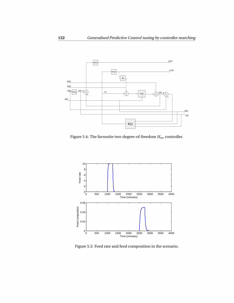
122 Generalised Predictive Control tuning by controller matching
P(z)∑ u(k)Wr(z)
Wu(z)
e1(k)
e2(k)
∑
Δ
∑
dy(k)
di(k)
y(k)r1(k)
We(z)
d(k)
d(k)
r(k)
r(k)
-+
K(z)
∑ +
-
Figure 5.4: The favourite two-degree-of-freedom H∞ controller.
0 500 1000 1500 2000 2500 3000 3500 40000
2
4
6
8
10
Time (minutes)
Fee
d ra
te
0 500 1000 1500 2000 2500 3000 3500 40000
0.02
0.04
0.06
Time (minutes)
Fee
d co
mpo
sitio
n
Figure 5.5: Feed rate and feed composition in the scenario.

5.6. Example 123
Table 5.5: Matrix P in the case of feed-forward control
0.0025 -0.0038 -0.0047 0.0071 0.0033 -0.0050 -0.0012 0.0017 0.0002 -0.00020.0011 -0.0006 -0.0020 0.0012 0.0014 -0.0008 -0.0005 0.0003 0.0001 -0.00000.0022 -0.0032 -0.0055 0.0081 0.0050 -0.0074 -0.0020 0.0030 0.0003 -0.00040.0010 -0.0006 -0.0024 0.0014 0.0022 -0.0013 -0.0009 0.0005 0.0001 -0.00010.0030 -0.0044 -0.0073 0.0108 0.0066 -0.0098 -0.0027 0.0040 0.0004 -0.00060.0014 -0.0008 -0.0033 0.0020 0.0030 -0.0018 -0.0012 0.0007 0.0002 -0.00010.0036 -0.0052 -0.0087 0.0127 0.0080 -0.0117 -0.0033 0.0049 0.0005 -0.00080.0017 -0.0010 -0.0041 0.0025 0.0037 -0.0022 -0.0015 0.0009 0.0002 -0.00010.0040 -0.0058 -0.0099 0.0144 0.0092 -0.0134 -0.0039 0.0056 0.0006 -0.00090.0019 -0.0012 -0.0048 0.0029 0.0044 -0.0027 -0.0018 0.0011 0.0003 -0.00020.0044 -0.0064 -0.0110 0.0159 0.0103 -0.0149 -0.0043 0.0063 0.0007 -0.00100.0022 -0.0014 -0.0054 0.0033 0.0050 -0.0031 -0.0021 0.0013 0.0003 -0.00020.0048 -0.0068 -0.0119 0.0171 0.0112 -0.0161 -0.0047 0.0068 0.0008 -0.00110.0024 -0.0015 -0.0059 0.0037 0.0055 -0.0035 -0.0023 0.0015 0.0004 -0.00020.0051 -0.0072 -0.0127 0.0182 0.0120 -0.0172 -0.0051 0.0073 0.0008 -0.00120.0026 -0.0016 -0.0064 0.0040 0.0061 -0.0038 -0.0026 0.0016 0.0004 -0.00030.0053 -0.0076 -0.0134 0.0191 0.0126 -0.0181 -0.0054 0.0077 0.0009 -0.00120.0028 -0.0018 -0.0069 0.0044 0.0065 -0.0041 -0.0028 0.0017 0.0004 -0.00030.0055 -0.0078 -0.0140 0.0198 0.0132 -0.0188 -0.0057 0.0080 0.0009 -0.00130.0029 -0.0019 -0.0073 0.0047 0.0069 -0.0044 -0.0029 0.0019 0.0005 -0.00030.0057 -0.0081 -0.0145 0.0205 0.0138 -0.0195 -0.0059 0.0083 0.0010 -0.00130.0031 -0.0020 -0.0077 0.0049 0.0073 -0.0047 -0.0031 0.0020 0.0005 -0.00030.0059 -0.0083 -0.0150 0.0211 0.0142 -0.0201 -0.0061 0.0086 0.0010 -0.00140.0032 -0.0021 -0.0081 0.0052 0.0076 -0.0049 -0.0033 0.0021 0.0005 -0.0003-0.0161 0.0248 0.0423 -0.0651 -0.0419 0.0644 0.0185 -0.0283 -0.0031 0.0047-0.0061 0.0033 0.0162 -0.0087 -0.0161 0.0087 0.0071 -0.0038 -0.0012 0.00060.0226 -0.0337 -0.0581 0.0868 0.0563 -0.0841 -0.0244 0.0365 0.0040 -0.00600.0099 -0.0058 -0.0254 0.0147 0.0245 -0.0142 -0.0106 0.0061 0.0017 -0.0010-0.0006 0.0016 0.0020 -0.0046 -0.0024 0.0051 0.0012 -0.0024 -0.0002 0.00040.0005 -0.0006 -0.0010 0.0012 0.0008 -0.0010 -0.0002 0.0004 0.0000 -0.00010.0042 -0.0057 -0.0103 0.0141 0.0096 -0.0132 -0.0040 0.0056 0.0006 -0.00090.0024 -0.0016 -0.0060 0.0040 0.0056 -0.0037 -0.0024 0.0016 0.0004 -0.00020.0042 -0.0057 -0.0104 0.0142 0.0097 -0.0132 -0.0041 0.0056 0.0006 -0.00090.0025 -0.0016 -0.0061 0.0040 0.0057 -0.0038 -0.0024 0.0016 0.0004 -0.0003
to 0.0329 [mole fraction] and that of the top composition is changed to 0.9706[mole fraction].
In this example, T (z ) = t (z )I2 with t (z ) = (1− 0.7z−1)5. The order of theopen-loop system is n = p + 1 = 4. Based on the dynamics of t (z ), the filterhorizon of the MV’s is H f = 12. The prediction horizon is chosen to be 17, ac-cording to Proposition 5.4.6 and also to cover the main dynamics of the system.According to Proposition 5.4.6, the filter horizon of the measured disturbancesis Hd = 6. The first step of the matching is to find KM P C such that the numer-ator and denominator of the MPC match those of the H∞ controller. MatricesP , Q and R are given in Tables 5.5, 5.6 and 5.7.
Since matrix [ P Q R ] is full column rank, the command \of MATLAB R©is used to solve the set of equations given in (5.39) to obtain KM P C , which is a2×34 matrix:
KM P C (:, 1 : 10) = 108
−0.0000 0.0000 −0.0000 0.0000 0.1304 −0.3189 0 0 −0.3238 0.7336−0.0000 0.0000 −0.0000 0.0000 0.1335 −0.2153 0 0 −0.3289 0.5031
KM P C (:, 11 : 20) = 108
0 0 0.1945 −0.4221 0.0010 −0.0068 0.0017 −0.0124 0.0030 −0.02220 0 0.1957 −0.2915 0.0002 −0.0035 0.0004 −0.0063 0.0008 −0.0114
KM P C (:, 21 : 30) = 108
−0.0919 0.5249 0.0530 −0.2562 −0.0232 0.1562 −0.0391 0.2614 −0.0654 0.4344−0.0843 0.3021 0.0437 −0.1473 −0.0258 0.0909 −0.0420 0.1512 −0.0680 0.2500
KM P C (:, 31 : 34) = 108
0.8856 −4.6233 −0.7258 3.55120.9616 −2.7647 −0.7870 2.1426
.

124 Generalised Predictive Control tuning by controller matching
Table 5.6: Matrix Q in the case of feed-forward control
-0.7649 0.0000 2.4135 0.0000 -2.6786 0.0000 1.2005 0.0000 -0.1681 0.00000.0000 -0.7649 0.0000 2.4135 0.0000 -2.6786 0.0000 1.2005 0.0000 -0.16810.3214 0.0000 -0.7767 0.0000 0.6257 0.0000 -0.1681 0.0000 0.0000 0.00000.0000 0.3214 0.0000 -0.7767 0.0000 0.6257 0.0000 -0.1681 0.0000 0.00000.1024 0.0000 -0.1734 0.0000 0.0734 0.0000 0.0000 0.0000 0.0000 0.00000.0000 0.1024 0.0000 -0.1734 0.0000 0.0734 0.0000 0.0000 0.0000 0.00000.1067 0.0000 -0.1813 0.0000 0.0770 0.0000 0.0000 0.0000 0.0000 0.00000.0000 0.1067 0.0000 -0.1813 0.0000 0.0770 0.0000 0.0000 0.0000 0.00000.1106 0.0000 -0.1884 0.0000 0.0802 0.0000 0.0000 0.0000 0.0000 0.00000.0000 0.1106 0.0000 -0.1884 0.0000 0.0802 0.0000 0.0000 0.0000 0.00000.1142 0.0000 -0.1949 0.0000 0.0831 0.0000 0.0000 0.0000 0.0000 0.00000.0000 0.1142 0.0000 -0.1949 0.0000 0.0831 0.0000 0.0000 0.0000 0.00000.1174 0.0000 -0.2008 0.0000 0.0858 0.0000 0.0000 0.0000 0.0000 0.00000.0000 0.1174 0.0000 -0.2008 0.0000 0.0858 0.0000 0.0000 0.0000 0.00000.1204 0.0000 -0.2062 0.0000 0.0883 0.0000 0.0000 0.0000 0.0000 0.00000.0000 0.1204 0.0000 -0.2062 0.0000 0.0883 0.0000 0.0000 0.0000 0.00000.1231 0.0000 -0.2111 0.0000 0.0905 0.0000 0.0000 0.0000 0.0000 0.00000.0000 0.1231 0.0000 -0.2111 0.0000 0.0905 0.0000 0.0000 0.0000 0.00000.1255 0.0000 -0.2156 0.0000 0.0925 0.0000 0.0000 0.0000 0.0000 0.00000.0000 0.1255 0.0000 -0.2156 0.0000 0.0925 0.0000 0.0000 0.0000 0.00000.1277 0.0000 -0.2196 0.0000 0.0943 0.0000 0.0000 0.0000 0.0000 0.00000.0000 0.1277 0.0000 -0.2196 0.0000 0.0943 0.0000 0.0000 0.0000 0.00000.1298 0.0000 -0.2233 0.0000 0.0960 0.0000 0.0000 0.0000 0.0000 0.00000.0000 0.1298 0.0000 -0.2233 0.0000 0.0960 0.0000 0.0000 0.0000 0.00000.1316 0.0000 -0.2267 0.0000 0.0975 0.0000 0.0000 0.0000 0.0000 0.00000.0000 0.1316 0.0000 -0.2267 0.0000 0.0975 0.0000 0.0000 0.0000 0.00000.1332 0.0000 -0.2297 0.0000 0.0989 0.0000 0.0000 0.0000 0.0000 0.00000.0000 0.1332 0.0000 -0.2297 0.0000 0.0989 0.0000 0.0000 0.0000 0.00000.1347 0.0000 -0.2324 0.0000 0.1001 0.0000 0.0000 0.0000 0.0000 0.00000.0000 0.1347 0.0000 -0.2324 0.0000 0.1001 0.0000 0.0000 0.0000 0.00000.1361 0.0000 -0.2349 0.0000 0.1012 0.0000 0.0000 0.0000 0.0000 0.00000.0000 0.1361 0.0000 -0.2349 0.0000 0.1012 0.0000 0.0000 0.0000 0.00000.1373 0.0000 -0.2372 0.0000 0.1023 0.0000 0.0000 0.0000 0.0000 0.00000.0000 0.1373 0.0000 -0.2372 0.0000 0.1023 0.0000 0.0000 0.0000 0.0000
Table 5.7: Matrix R in the case of feed-forward control
0.0012 0.2460 -0.0011 -0.2166 0.0000 0.0000 0.0000 0.0000 0.0000 0.0000-0.0000 0.0733 0.0000 -0.0594 0.0000 0.0000 0.0000 0.0000 0.0000 0.00000.0022 0.4561 -0.0051 -1.0395 0.0041 0.8437 -0.0014 -0.2953 0.0002 0.0413-0.0000 0.1411 0.0001 -0.3138 -0.0001 0.2514 0.0000 -0.0880 -0.0000 0.01230.0031 0.6359 -0.0071 -1.4609 0.0062 1.2692 -0.0025 -0.5062 0.0004 0.0767-0.0001 0.2037 0.0001 -0.4591 -0.0001 0.3960 0.0001 -0.1571 -0.0000 0.02370.0038 0.7899 -0.0090 -1.8689 0.0081 1.6749 -0.0033 -0.6867 0.0005 0.1069-0.0001 0.2613 0.0001 -0.6081 -0.0001 0.5415 0.0001 -0.2208 -0.0000 0.03420.0044 0.9222 -0.0106 -2.2190 0.0097 2.0228 -0.0040 -0.8415 0.0006 0.1328-0.0000 0.3142 0.0001 -0.7451 -0.0001 0.6754 0.0001 -0.2794 -0.0000 0.04390.0049 1.0358 -0.0119 -2.5197 0.0110 2.3215 -0.0046 -0.9743 0.0007 0.1550-0.0000 0.3628 0.0001 -0.8709 -0.0001 0.7984 0.0000 -0.3333 -0.0000 0.05280.0053 1.1336 -0.0130 -2.7785 0.0121 2.5784 -0.0051 -1.0885 0.0008 0.1741-0.0000 0.4073 0.0001 -0.9862 -0.0001 0.9111 0.0000 -0.3827 -0.0000 0.0610-0.0272 -5.4667 0.0664 13.3758 -0.0620 -12.4858 0.0260 5.2331 -0.0041 -0.83080.0008 -1.5443 -0.0020 3.7894 0.0019 -3.5414 -0.0008 1.4854 0.0001 -0.23590.0260 5.2726 -0.0627 -12.6767 0.0575 11.6372 -0.0239 -4.8331 0.0038 0.7620-0.0007 1.5313 0.0018 -3.6696 -0.0016 3.3640 0.0007 -1.3958 -0.0001 0.2199-0.0044 -0.8443 0.0108 2.0722 -0.0102 -1.9590 0.0043 0.8208 -0.0007 -0.13020.0002 -0.1760 -0.0006 0.4471 0.0005 -0.4308 -0.0002 0.1823 0.0000 -0.02910.0016 0.3556 -0.0036 -0.8076 0.0030 0.6862 -0.0012 -0.2764 0.0002 0.04260.0000 0.1548 -0.0001 -0.3467 0.0001 0.2981 -0.0000 -0.1200 0.0000 0.01850.0016 0.3579 -0.0036 -0.8134 0.0030 0.6909 -0.0012 -0.2783 0.0002 0.04290.0000 0.1572 -0.0001 -0.3521 0.0001 0.3028 -0.0000 -0.1219 0.0000 0.01880.0016 0.3601 -0.0036 -0.8187 0.0030 0.6952 -0.0012 -0.2800 0.0002 0.04320.0000 0.1593 -0.0001 -0.3570 0.0001 0.3070 -0.0000 -0.1236 0.0000 0.01910.0016 0.3620 -0.0036 -0.8233 0.0030 0.6989 -0.0012 -0.2815 0.0002 0.04340.0000 0.1613 -0.0001 -0.3615 0.0001 0.3109 -0.0000 -0.1252 0.0000 0.01930.0016 0.3637 -0.0036 -0.8274 0.0030 0.7023 -0.0012 -0.2829 0.0002 0.04360.0001 0.1630 -0.0001 -0.3655 0.0001 0.3143 -0.0000 -0.1266 0.0000 0.01950.0016 0.3652 -0.0036 -0.8311 0.0031 0.7053 -0.0012 -0.2841 0.0002 0.04380.0001 0.1646 -0.0001 -0.3691 0.0001 0.3175 -0.0000 -0.1279 0.0000 0.01970.0016 0.3665 -0.0036 -0.8344 0.0031 0.7079 -0.0012 -0.2852 0.0002 0.04400.0001 0.1660 -0.0001 -0.3724 0.0001 0.3203 -0.0000 -0.1290 0.0000 0.0199

5.7. Conclusion and future work 125
0 500 1000 1500 2000 2500 3000 3500 40000.94
0.96
0.98
1Top composition
Time (minutes)
Mol
e fr
actio
n
0 500 1000 1500 2000 2500 3000 3500 40000
0.02
0.04
0.06
0.08
0.1Bottom composition
Time (minutes)
Mol
e fr
actio
n
MPCHinf
Figure 5.6: Closed loop response of the controlled variables (top and bottomcompositions) for MPC, (-) and for H∞,(- -) .
With this KM P C , the convex optimisation problem (5.51) is solved with theKM P C divided by a scale factor of 105. All the weighting matrices are full ma-trices of real elements and given in Appendix B.4. The 2-norm of the error be-tween the unscaled KM P C and:
H >Qne w H +R+ H >Sne w +S>ne w H−1
H >Qne w +S>ne w
(5.71)
is 0.0163. The outputs and inputs of the H∞ controller and the MPC is given inFigures 5.6 and 5.7, respectively. It can be seen that two controllers match wellwhen the constraints are inactive.
5.7 Conclusion and future work
A tuning method for MPC based on controller matching is proposed. The MPCis formulated in the transfer function form. The main idea of the method is tomatch the transfer function of an arbitrary favourite controller and the MPC.Provided that some rank conditions are satisfied, perfect matching betweenthe two controllers can be obtained when the constraints are inactive. Thematching can also be done with feed-forward control in the favourite controller.

126 Generalised Predictive Control tuning by controller matching
0 500 1000 1500 2000 2500 3000 3500 4000520
540
560
580
600Liquid flowrate
Time (minutes)
Km
ol/m
in
0 500 1000 1500 2000 2500 3000 3500 4000660
680
700
720
740Vapour flowrate
Time (minutes)
Km
ol/m
in
MPCHinf
Figure 5.7: Closed loop response of the manipulated variables (liquid andvapour flowrates) for MPC, (-) and for H∞,(- -) .
The use of T (z ) helps to fulfill the rank conditions while T (z )−1 remains a low-pass filter. Two main steps are followed in the matching. The first step is tofind a gain KM P C that matches the transfer function given. The second step isto find the tuning parameters by formulating a convex optimisation problemwith LMI constraints.
The filter T (z )−1 is usually a low-pass filter whose bandwidth is preferredto be higher than that of the model. In this work, T (z ) is selected based onthe engineering rules given in Rossiter (2005). It should be noted that H f andT (z ) also affect the quality of the prediction. A fast T (z )will allow a low H f butmay cause numerical issues since the coefficients of T (z ) will become small.Therefore, a more analytical approach to the computation of T (z ) should beconsidered in future work.
Regarding optimisation problem (5.51), in Cairano and Bemporad (2010),raising the prediction horizon is a method to increase the degrees of freedomin the LMI to obtain a lower error when matching the state feedback gain. Nev-ertheless, this work and Shah and Engell (2010, 2011, 2013) solve the matchingof the output feedback gain KM P C , whose size depends on the prediction hori-zon. This is a fundamental difference that limits the benefit gained by increas-ing the prediction horizon to obtain more degrees of freedom. As shown in
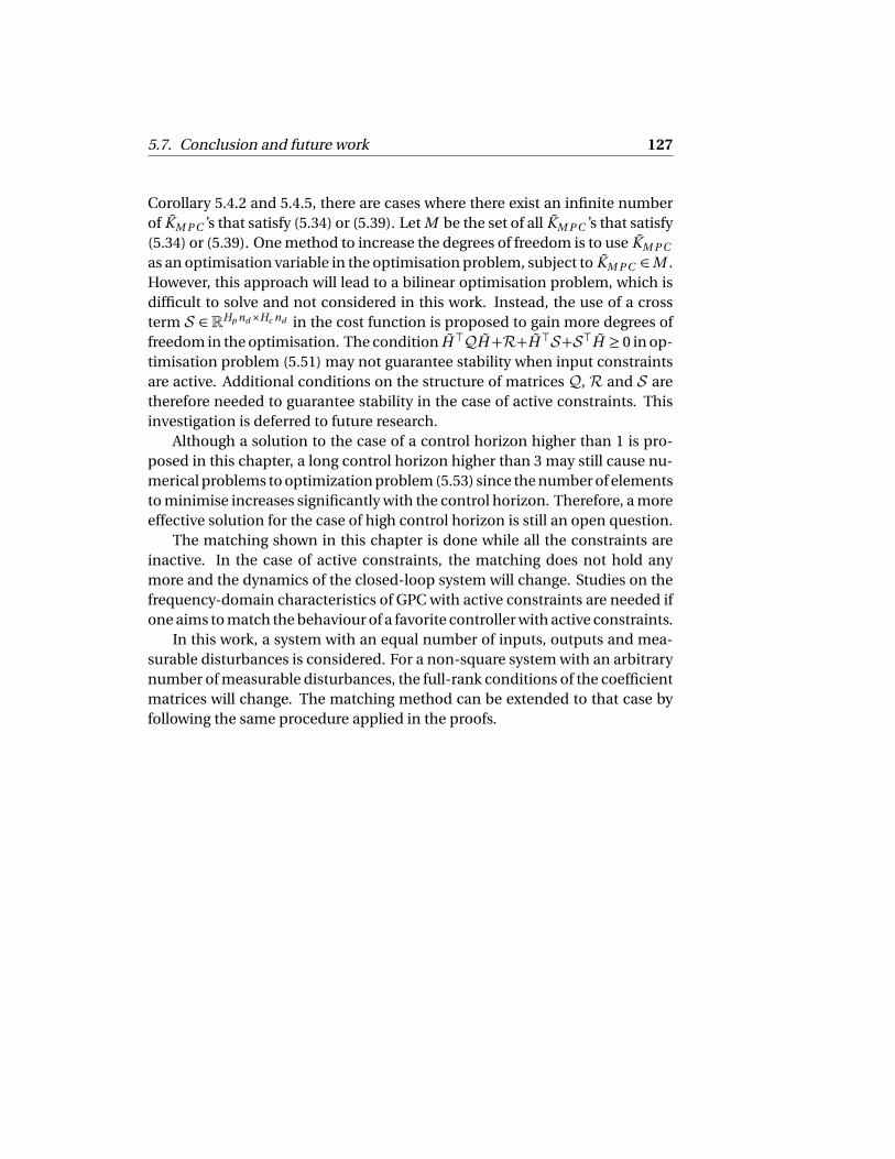
5.7. Conclusion and future work 127
Corollary 5.4.2 and 5.4.5, there are cases where there exist an infinite numberof KM P C ’s that satisfy (5.34) or (5.39). Let M be the set of all KM P C ’s that satisfy(5.34) or (5.39). One method to increase the degrees of freedom is to use KM P C
as an optimisation variable in the optimisation problem, subject to KM P C ∈M .However, this approach will lead to a bilinear optimisation problem, which isdifficult to solve and not considered in this work. Instead, the use of a crossterm S ∈ RHp nd×Hc nd in the cost function is proposed to gain more degrees offreedom in the optimisation. The condition H >QH +R+H >S+S>H ≥ 0 in op-timisation problem (5.51) may not guarantee stability when input constraintsare active. Additional conditions on the structure of matrices Q, R and S aretherefore needed to guarantee stability in the case of active constraints. Thisinvestigation is deferred to future research.
Although a solution to the case of a control horizon higher than 1 is pro-posed in this chapter, a long control horizon higher than 3 may still cause nu-merical problems to optimization problem (5.53) since the number of elementsto minimise increases significantly with the control horizon. Therefore, a moreeffective solution for the case of high control horizon is still an open question.
The matching shown in this chapter is done while all the constraints areinactive. In the case of active constraints, the matching does not hold anymore and the dynamics of the closed-loop system will change. Studies on thefrequency-domain characteristics of GPC with active constraints are needed ifone aims to match the behaviour of a favorite controller with active constraints.
In this work, a system with an equal number of inputs, outputs and mea-surable disturbances is considered. For a non-square system with an arbitrarynumber of measurable disturbances, the full-rank conditions of the coefficientmatrices will change. The matching method can be extended to that case byfollowing the same procedure applied in the proofs.

128 Generalised Predictive Control tuning by controller matching

6A fresh perspective on the connection between
the frequency and nite time domains
6.1 Introduction6.2 Preliminaries and review
of relevant developments
6.3 New results on the relationbetween finite timedomain and frequency domain
6.4 Conclusion and future work
6.1 Introduction
In the previous chapters, the tuning methods based on controller matching areconsidered. Such methods often include multiple stages. A matching methodin the state-space formulation requires the observer-based realisation to ex-tract the static control gain. A matching method for the GPC requires solvinga set of linear equations and an optimisation problem to find the weightingmatrices. Furthermore, an optimisation problem cannot guarantee a solutionand the observer-based realisation can restrict the dynamics of the observer.For those reasons, a more direct approach to the tuning that can directly usethe frequency-domain properties of the system is desirable. In order to buildsuch a tuning approach, the connection between the finite-time-domain MPCtechnology and the frequency domain needs to be analysed. The vision of thiswork is to understand this connection when the horizons are finite.
While the receding horizon principle and the constraints handling are thetime-domain features of MPC, the basic frequency-domain feature of MPC is

130A fresh perspective on the connection between the frequency and finite time
domains
Q(z)∑
-+yr (k)
dy(k)
y(k)
∑ M(z)
P(z) ∑ +
+
+-
u(k)
d(k)
Figure 6.1: IMC scheme.
that it is an inverse-based controller. When the horizons are infinite and noweight is imposed on the input signals, MPC produces a controller equivalentto the inverse of the process at all frequencies. A change in the weighting ma-trices of MPC can be translated into the limitation in the frequency range inwhich the process is inverted. The feedback scheme that reflects the inverse-based controller is the IMC scheme given in Figure 6.1, where d y (k ) is the out-put disturbance, P (z ) is the plant, M (z ) is the model, Q (z ) can be any stablesystem and d (k ) = d y (k ) + (P (z )−M (z ))u (k ). Although Q (z ) can be any sta-ble system, the optimal LQ solution is equivalent to a Q (z ) that is the inverseof the outer part of the process. This fact directly relates the closed-loop be-haviour of the system to the invertibility of the process. It can give insight intohow the process characteristics limit the behaviour of the controller. Hence, away of analysing the tuning of the controller is to find the direct link betweentuning and the frequency range in which the process is inverted. This analysisalso allows us to directly connect the open-loop properties of the plant to thebehaviour of the closed-loop system.
In MPC, the inversion of the process is reflected in the inversion of the so-called system matrix, which is mentioned in the literature review in Chapter1. When no input weight is used, the Toeplitz matrix, which links the futureoutputs and future inputs, is inverted in calculating the MPC solution. In liter-ature, it is shown that the singular values of the Toeplitz matrix approach thefrequency-domain magnitude of the open-loop system. In this work, we showthat each singular vector is a sine wave corresponding to 1 frequency point inthe range [0;π] rad/s, assuming that the sampling period is 1 second. This factgives the intuition that limiting the singular values in the inversion can produce

6.2. Preliminaries and review of relevant developments 131
the similar limitation in the frequency range in which the process is inverted.However, we show that manipulating the singular values of the Toeplitz matrix(e.g. setting some of them to 0) does not simply produce the same effect inthe Bode plot of the controller. This phenomenon is due to the finite horizons.Therefore, this chapter provides further analysis of the connection between theToeplitz matrix and the frequency-domain properties of the system.
This chapter is organised as follows. Section 6.2 provides a review of therelevant developments, including the MPC formulated with FIR models andthe preliminary results in literature. Section 6.3 presents further analysis of theconnection between the finite time domain and frequency domain. This in-cludes the connection between the singular vectors of the Toeplitz matrix andthe phase and directionality of the open-loop system, followed by the finite-time behaviour of the Toeplitz and Hankel matrices. Concluding commentsand future research directions are given in Section 6.4.
6.2 Preliminaries and review of relevant developments
Initial studies towards the connection between the finite time domain and fre-quency domain were undertaken in Goodwin et al. (2005), Rojas et al. (2003,2004) and Rojas and Goodwin (2004). They showed the link between the sin-gular values of the Hessian matrix, which is the square of the Toeplitz matrix,and the gain of the open-loop system in the frequency domain. The use of theSVD of the Toeplitz matrix for analysing the finite-time behaviour of systems isalso considered in Ludlage (1997) and Ludlage et al. (2003). In those works, thistechnique was used to investigate the controllability of systems and the non-minimum phase phenomenon. In Maurath et al. (1988b), the link between theSVD of the matrix that is inverted in the computation of the MPC solution andthe weighting matrices is provided. This is the basis in their tuning method,which is based on the contribution of the singular values to the cost function.However, no connection to the frequency-domain characteristics of the systemwas made in that work.
In this section, the fact that any weighting matrices Q and R can be trans-lated into changes in the singular values matrix of the Toeplitz matrix is shownbased on Maurath et al. (1988b). This section also replicates an example inGoodwin et al. (2005). The intention of the work in Goodwin et al. (2005) is toprovide a control strategy that limits the inversion of the plant when the sys-tem operates closely to the constraints. This is done by limiting the singularvalues of the Toeplitz matrix. We show that the connection between the sin-gular values of the Toeplitz matrix and the closed-loop bandwidth provided in

132A fresh perspective on the connection between the frequency and finite time
domains
Goodwin et al. (2005) is incomplete.That work has motivated us to do further analysis of the connection be-
tween the time domain and frequency domain. The long-term objective of thisanalysis is to build a tuning method based on frequency-domain techniqueswhich can also tackle constraints in an explicit way. The design of such a tun-ing method, however, is beyond the scope of this thesis due to time limitation.
6.2.1 MPC based on FIR models
This subsection first shows that any change in the input penalty of MPC canbe translated as a change in the singular value matrix of the Toeplitz matrix.The MPC based on FIR models is translated into the IMC controller when con-straints are inactive. This allows the analysis of the frequency-domain proper-ties of the controller designed based on the singular values of the Toeplitz ma-trix. The design of Goodwin et al. (2005), which explicitly takes into accountthe constraints of the system, is then presented and analysed.
The Toeplitz and Hankel matrices are used in the prediction of the MPCformulated in FIR models. The Toeplitz matrix represents the effect of futureinputs on future outputs and the Hankel matrix represents the effect of pastinputs on future outputs. In this work, only stable systems are considered. As-sume also that the system is square: nu = ny . Let Mk be the kth element ofthe impulse response of the system. For a stable system, there exists a finite k0
such that Mk ≈ 0 for k > k0. Therefore, the FIR model is given by:
y (k ) =k0∑
i=0
Mi u (k − i ). (6.1)
Let Hp denote the prediction horizon and Hu denote the control horizon, thepredicted output is:
Yf = T Uf +H Up +
d (k )d (k )
...d (k )
(6.2)
where Yf is the future output vector, Uf and Up are the future and past inputvectors, respectively:

6.2. Preliminaries and review of relevant developments 133
Yf =
y (k )y (k +1)
...y (k +Hp −2)y (k +Hp −1)
; Uf =
u (k )u (k +1)
...u (k +Hu −2)u (k +Hu −1)
; Up =
u (k −Hp a s t )...
u (k −2)u (k −1)
(6.3)
T is the Toeplitz matrix
T =
M0 0 . . 0M1 M0 0 . .M2 M1 M0 . .
. . . . 0MHu−1 MHu−2 MHu−3 . M0
MHuMHu−1 MHu−2 . M1
. . . . .MHp−1 MHp−2 MHp−3 . MHp−Hu
(6.4)
H is the Hankel matrix
H =
MHp a s t. . M2 M1
MHp a s t+1 . . M3 M2
. . . . .
. . . . .MHp a s t+Hp−1 . . MHp+1 MHp
(6.5)
Hp a s t is the past horizon and d (k ) is the feedback term:
d (k ) = yme a s u r e d (k )− ymo d e l (k ) (6.6)
Since Mk ≈ 0 for k > k0, it is sensible to select Hp a s t = k0. However, the notationHp a s t is still used in the following for clarity. For the sake of simplicity, thecontrol horizon is considered equal to the prediction horizon: Hp =Hu =N .
Assume that the aim of the controller at time instant k is to steer the outputof the system to a reference yr (k ). The control action is obtained from the so-lution to the following optimisation problem at time instant k , assuming thatthe weighting matrix on the output errors is identity:

134A fresh perspective on the connection between the frequency and finite time
domains
minUf
Yf −
yr (k )yr (k +1)
...yr (k +N −1)
>
Yf −
yr (k )yr (k +1)
...yr (k +N −1)
+
Uf −
us s
us s...
us s
>
R
Uf −
us s
us s...
us s
(6.7)
where
yr (k )yr (k +1)
...yr (k +N −1)
is the prediction of the output reference and us s =
G −1M
yr (k )−d (k )
where GM is the steady-state gain matrix of the open-loopsystem. Note that the MPC cost function above penalises the deviations ofthe inputs from their steady-state values instead of the input changes. Usuallywhen no reference trajectory is used,
yr (k ) = yr (k +1) = . . .= yr (k +N −1). (6.8)
Let Us s denote matrix
us s
us s...
us s
with the appropriate dimension, the control
input sequence is then given by:
u (k )u (k +1)
...u (N −1)
=−
T >T +R−1
T >
H Up −Yr e f +D
−RUs s
. (6.9)
where Yr e f =
yr (k )yr (k )
...yr (k )
and D =
d (k )d (k )
...d (k )
. Since us s =G −1M
yr (k )−d (k )
, it is
obvious that:

6.2. Preliminaries and review of relevant developments 135
T
us s
us s...
us s
+H
us s
us s...
us s
= Yr e f −D . (6.10)
The control sequence then becomes:
Uf =−
T T T +R−1
T T H
Up −Us s
+Us s . (6.11)
Consider the SVD of the Toeplitz matrix T :
T =UT SV >T (6.12)
=
uT11uT12
· · · uT1N
uT21uT22
· · · uT2N
......
...uTN 1
uTN 2· · · uTN N
s1
s2
...sN
vT11vT12
· · · vT1N
vT21vT22
· · · vT2N
......
...vTN 1
vTN 2· · · vTN N
>
.
(6.13)
The control input sequence then becomes:
Uf =−
VT S 2V >T +R−1
VT SU >T H
Up −Us s
+Us s . (6.14)
Let R2 =VT RV >T , it follows that:
Uf =−VT
S 2+R2
−1SU >
T H
Up −Us s
+Us s (6.15)
=−T H
Up −Us s
+Us s . (6.16)
This shows that any change made in the penalty input R can be translated intoa change in the singular value matrix of the Toeplitz matrix T . When R = 0, Tbecomes the pseudo-inverse of T . Let
T =
t11 t12 · · · t1N
t21 t22 · · · t2N...
......
...tN 1 tN 2 · · · tN N
. (6.17)
Since the MPC only implements the first nu sample of Uf in the system, theactual control action at time instant k is given by:

136A fresh perspective on the connection between the frequency and finite time
domains
u (k ) =−
t11 t12 · · · t1N
H
Up −Us s
+us s . (6.18)
Let
K =
t11 t12 · · · t1N
H (6.19)
=
kNp a s tkNp a s t−1 · · · k1
(6.20)
it follows that:
u (k ) =−K
u (k −Np a s t )...
u (k −2)u (k −1)
+ L
yr (k )−d (k )
(6.21)
where L =
Inu+K
Inu
Inu...
Inu
G −1M . The transfer function from yr (k )−d (k ) to
u (k ) is then given by
u (k ) =
Inu+k1z−1+k2z−2+ . . .+kNp a s t
z−Np a s t
−1L
yr (k )−d (k )
(6.22)
This is the transfer function of the IMC controller Q (z ) shown in Figure 6.1. LetGQ denote the steady-state gain of Q (z ) and yr s s denote the steady-state valueof the output reference. Transfer function (6.22) of Q (z ) shows that GQ =G −1
M .The IMC scheme in Figure 6.1 gives the following steady-state relation:
us s =GQ
yr s s −
ys s −GM us s
(6.23)
=GQ yr s s −GQ ys s +GQ GM us s (6.24)
=GQ yr s s −GQ ys s +us s (6.25)
⇒ yr s s = ys s . (6.26)
Therefore, the steady-state gain of Q (z ) ensures the integral action of the con-troller. The controller Q (z ) in the IMC scheme is used to analyse the frequencydomain properties of the tuning method proposed by Goodwin et al. (2005).

6.2. Preliminaries and review of relevant developments 137
6.2.2 MPC tuning based on the singular values of the Toeplitz matrix
In this subsection, the tuning method presented in Goodwin et al. (2005) isdescribed. The main idea of the method is to assign the smallest singular valuesof the Toeplitz matrix to zeros in order to respect the constraints as well as torestrict the closed-loop bandwidth of the system. Consider the case where R2
in (6.15) is 0, (6.16) can be written as:
Uf =−VT Z U >T H
Up −Us s
+Us s (6.27)
where Z = S−1 =
z1 0 · · · 0
0 z2...
......
...... 0
0 · · · 0 zN
and z1 ¾ z2 ¾ . . . ¾ zN . The tuning
algorithm presented in Goodwin et al. (2005) includes the following steps:
1. At time instant k , the unconstrained MPC input sequence is calculated:
Uf =−VT
z1 0 · · · 0
0 z2...
......
...... 0
0 · · · 0 zN
U >T H
Up −Us s
+Us s . (6.28)
2. Find the largest r where r ∈ 1, 2, . . . , N nu and nu is the number of in-puts, such that vector
Uf SV D =−VT diag (z1, z2, . . . , zr , 0, . . . , 0)U >T H
Up −Us s
+Us s (6.29)
satisfies the constraints of the system.
3. Implement the first nu elements of the control sequence to the system.
4. Increase k by 1 and return to step 1.
More details and mathematical expressions of the tuning strategy and the sta-bility analysis can be found in Goodwin et al. (2005). The focus of this chapteris the frequency-domain properties of a controller designed with this method.
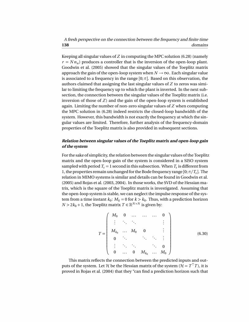
138A fresh perspective on the connection between the frequency and finite time
domains
Keeping all singular values of Z in computing the MPC solution (6.28) (namelyr = N nu ) produces a controller that is the inversion of the open-loop plant.Goodwin et al. (2005) showed that the singular values of the Toeplitz matrixapproach the gain of the open-loop system when N →∞. Each singular valueis associated to a frequency in the range [0;π]. Based on this observation, theauthors claimed that assigning the last singular values of Z to zeros was simi-lar to limiting the frequency up to which the plant is inverted. In the next sub-section, the connection between the singular values of the Toeplitz matrix (i.e.inversion of those of Z ) and the gain of the open-loop system is establishedagain. Limiting the number of non-zero singular values of Z when computingthe MPC solution in (6.28) indeed restricts the closed-loop bandwidth of thesystem. However, this bandwidth is not exactly the frequency at which the sin-gular values are limited. Therefore, further analysis of the frequency-domainproperties of the Toeplitz matrix is also provided in subsequent sections.
Relation between singular values of the Toeplitz matrix and open-loop gainof the system
For the sake of simplicity, the relation between the singular values of the Toeplitzmatrix and the open-loop gain of the system is considered in a SISO systemsampled with period Ts = 1 second in this subsection. When Ts is different from1, the properties remain unchanged for the Bode frequency range [0;π/Ts ]. Therelation in MIMO systems is similar and details can be found in Goodwin et al.(2005) and Rojas et al. (2003, 2004). In those works, the SVD of the Hessian ma-trix, which is the square of the Toeplitz matrix is investigated. Assuming thatthe open-loop system is stable, we can neglect the impulse response of the sys-tem from a time instant k0: Mk = 0 for k > k0. Thus, with a prediction horizonN > 2k0+1, the Toeplitz matrix T ∈RN×N is given by:
T =
M0 0 . . . . . . . . . 0...
......
...
Mk0. . . M0 0
...
0...
......
......
......
... 00 . . . 0 Mk0
. . . M0
(6.30)
This matrix reflects the connection between the predicted inputs and out-puts of the system. Let H be the Hessian matrix of the system (H = T >T ), it isproved in Rojas et al. (2004) that they “can find a prediction horizon such that

6.2. Preliminaries and review of relevant developments 139
there exists at least one singular value ofH that is arbitrarily close to the energydensity spectrum Φ(.) of the system [at some frequency ω0]". In other words,the following equality holds:
‖Hw Nl −Φ(ω0)w
Nl ‖2 −→ 0 when N →∞ (6.31)
where w Nl is the following vector:
w Nl =
1p
N[1 e − j 2π
N l e − j 2πN 2l . . . e − j 2π
N (N−1)l ]> (6.32)
with l ∈Z such that 0≤ l ≤N −1 and ‖w Nl ‖2 = 1. Then, l is proved to be (Nω0)/
(2π) (when l varies from 0 to N −1,ω0 varies from 0 to 2π(N −1)/N → 2πwhenN →∞ ).
Equality (6.31) shows that the energy density spectrum Φ(.) of the systemis the eigenvalues of the Hessian matrix. The Hessian matrix is the square ofthe Toeplitz matrix and therefore the eigenvectors of the Hessian matrix arethe singular vectors of the Toeplitz matrix and the eigenvalues of the Hessianmatrix are the square of the singular values of the Toeplitz matrix. Furthermore,the relation between the energy density spectrum Φ(ω) and the amplitude ofthe system |G (e jω)| is given by:
p
Φ(ω) = |G (e jω)|. (6.33)
Therefore, the singular values of the Toeplitz matrix converge to the amplitudeof the open-loop system. Due to this relation and the fact that the solution ofMPC given in (6.28) inverts the Toeplitz matrix when no input weight is used,Goodwin et al. (2005) suggested that when one limits the number of singularvalues inverted in that solution, the frequency to which the singular values arelimited corresponds to the frequency to which the process is inverted in thecontroller. The following example shows that this intuition is in fact incom-plete.
Example
The same example as the one used in Section 11.7, Chapter 11 of Goodwin et al.(2005) is used in this subsection. Consider the system
x (t ) =−x (t ) +u (t )
y (t ) = x (t )(6.34)

140A fresh perspective on the connection between the frequency and finite time
domains
100
101
102
103
10−20
10−15
10−10
10−5
100
Singular values of the Toeplitz matrix & magnitude of the open−loop system
Frequency (rad/s)
Singular valuesMagnitude
Figure 6.2: The singular values of the Toeplitz matrix match the magnitude ofthe open-loop system.
sampled with period Ts = 0.025 second. The control objective of the system isto steer y (t ) to 1. The set-point changes from 0 to 1 at 0.1 second. First, weshow that the singular values of the Toeplitz matrix match the open-loop gainof the system. Then we investigate the relation between the closed-loop band-width of the system and the number of singular values assigned to zeros whenMPC solution is computed. For this purpose, no constraint is considered in theexample and therefore the number of non-zero singular values in calculatingthe MPC solution is fixed. As in Goodwin et al. (2005), the prediction horizonN = 251 is equal to the control horizon, which is 6.25 seconds. The singularvalues of the Toeplitz matrix and the corresponding gain of the open-loop sys-tem are given in Figure 6.2. Figure 6.2 shows that the singular values indeedmatch the open-loop gain of the system. Note that the frequency range is from0 toπ/Ts . The zero singular value on the figure is due to the fact that the systemis strictly proper and the Toeplitz matrix is rank-deficient.
Consider a controller obtained from (6.28) with zk = 0 for k ≥ 22. The fre-quency corresponding to z21 is approximately 10.4 rad/s. The closed-loop re-sponse of the input and output signals are given in Figures 6.3a and 6.3b, re-spectively. These responses are identical to those given in Subsection 11.7.2,Chapter 11 of Goodwin et al. (2005). Based on the calculation described inSection 6.2.1, the transfer function of the corresponding IMC controller is com-puted, and the Bode plot of the product Q (z )M (z ) is given in Figure 6.4. Since

6.2. Preliminaries and review of relevant developments 141
0 0.5 1 1.5 20
1
2
3
4
5
6
7Control input
Time (seconds)
(a) Input signal of the system.
0 0.5 1 1.5 2 2.50
0.1
0.2
0.3
0.4
0.5
0.6
0.7
0.8
0.9
1Controlled output
Time (seconds)
(b) Output signal of the system.
Figure 6.3: Closed-loop response of the system when 21 largest singular valuesof the Toeplitz matrix are inverted.
−25
−20
−15
−10
−5
0
Mag
nitu
de (
dB)
System: untitled1Frequency (rad/s): 1.84Magnitude (dB): −0.267
System: untitled1Frequency (rad/s): 7.34Magnitude (dB): −3.03
10−1
100
101
102
103
−225
−180
−135
−90
−45
0
Pha
se (
deg)
Bode Diagram
Frequency (rad/s)
Figure 6.4: Bode plot of Q (z )M (z ) when 21 largest singular values of theToeplitz matrix are inverted.
no model-plant mismatch is present in this example, Figure 6.4 shows that thecontroller is the perfect inverse of the plant up to approximately 1.84 rad/s.After this frequency, the magnitude of the Bode plot shows a smooth roll-offinstead of a sudden change to 0 as in the singular values.
Now consider a controller obtained from (6.28) with zk = 0 for k < 40. Thisselection is used to show that although the singular values corresponding tolow frequencies are 0, the product Q (z )M (z ) does not show high-pass char-acteristics. The corresponding input and output signals are given in Figure

142A fresh perspective on the connection between the frequency and finite time
domains
0 0.5 1 1.5 20
5
10
15
20
25
30Control input
Time (seconds)
(a) Input signal of the system.
0 0.5 1 1.5 20
0.1
0.2
0.3
0.4
0.5
0.6
0.7
0.8
0.9
1Controlled output
Time (seconds)
(b) Output signal of the system.
Figure 6.5: Closed-loop response of the system when 39 largest singular valuesof the Toeplitz matrix are set to 0.
6.5a and 6.5b, respectively. The Bode plot of Q (z )M (z ) is given in Figure 6.6. Itshows a low-pass characteristics with very mild roll-off. This can be explainedby the fact that the small singular values of the Toeplitz matrix are kept in theinversion, which leads to a large control signal and the plant is also invertedat high frequencies. Although the singular values at low frequencies are setto 0, the product of the controller and the process still exhibits a low-pass be-haviour. That is to say, the direct connection between the singular values andthe frequency-domain properties is missing.
6.3 New results on the relation between finite time do-main and frequency domain
Goodwin et al. (2005) used the information related to the gain of the system(i.e. the singular values) to influence the controller design. The question iswhether it is possible to obtain the phase and directionality information fromthe Toeplitz matrix and use it. In subsection 6.3.1, we present our research ef-forts in analysing the asymptotic behaviour of the Toeplitz matrix. Section 6.3.2discusses the results of considering the finite-time behaviour of the Toeplitzand Hankel matrices.

6.3. New results on the relation between finite time domain and frequencydomain 143
−6
−5
−4
−3
−2
−1
0
Mag
nitu
de (
dB)
System: untitled1Frequency (rad/s): 3.57Magnitude (dB): −0.0465
System: untitled1Frequency (rad/s): 59.9Magnitude (dB): −3.03
10−1
100
101
102
103
−180
−135
−90
−45
0
Pha
se (
deg)
Bode Diagram
Frequency (rad/s)
Figure 6.6: Bode plot of Q (z )M (z ) when 39 largest singular values of theToeplitz matrix are set to 0.
6.3.1 Asymptotic connection between SVD of the Toeplitz matrix andBode plot of the open-loop system
In this subsection, it is shown that the phase and directionality information ofthe open-loop system can also be found in the SVD of the Toeplitz matrix whenN →∞.
SISO case
Note that the Toeplitz matrix and the Hessian matrix consist of real numbersand in fact their singular vectors also include real numbers. In the following,we present the real singular vectors of the Toepliz matrix. We show that (6.31)holds for the following real vector:
v Nl =
1
L[cos(
π
N +1l +ϕl ) cos(
π
N +12l +ϕl ) . . . cos(
π
N +1N l +ϕl )]
> (6.35)
with ϕl ∈ R, l ∈ Z, 1 ≤ l ≤ N , and L =p
(N − cos(2ϕl ))/2; and vector (6.35) isthe actual singular vector of the Toeplitz matrix. We put forward the followingtheorem for further calculation in the proofs.
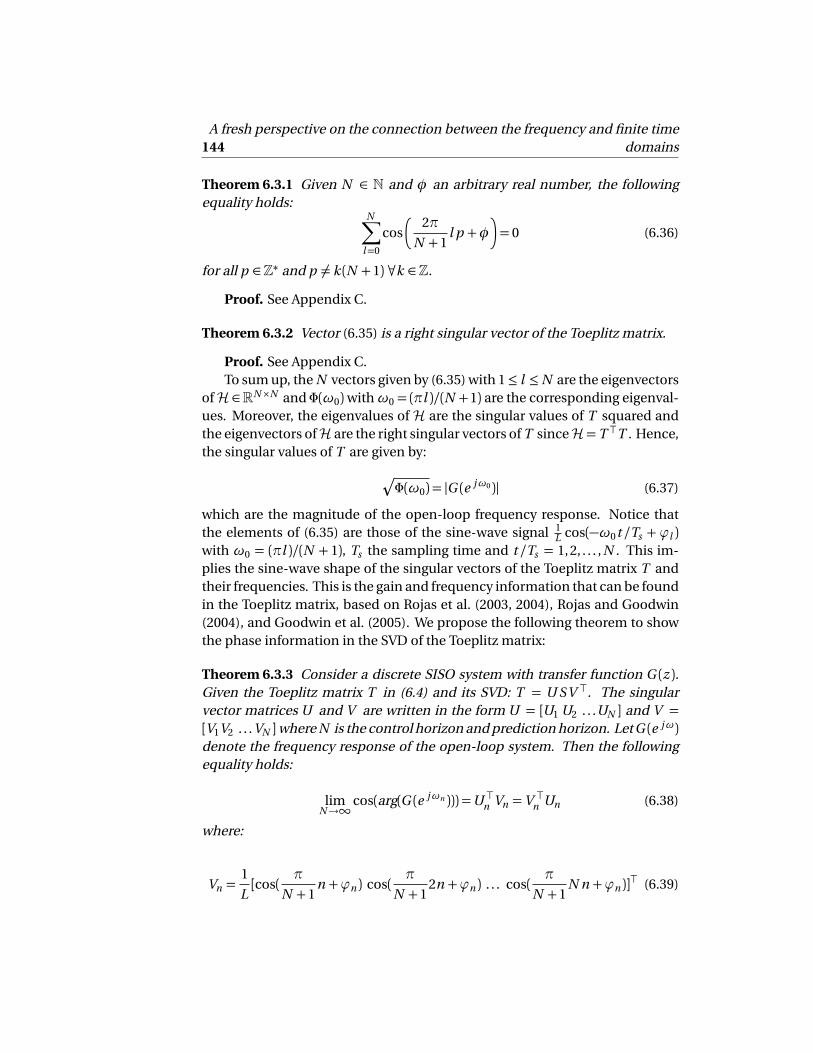
144A fresh perspective on the connection between the frequency and finite time
domains
Theorem 6.3.1 Given N ∈ N and φ an arbitrary real number, the followingequality holds:
N∑
l=0
cos
2π
N +1l p +φ
= 0 (6.36)
for all p ∈Z∗ and p 6= k (N +1) ∀k ∈Z.
Proof. See Appendix C.
Theorem 6.3.2 Vector (6.35) is a right singular vector of the Toeplitz matrix.
Proof. See Appendix C.To sum up, the N vectors given by (6.35) with 1≤ l ≤N are the eigenvectors
of H ∈RN×N and Φ(ω0)withω0 = (πl )/(N +1) are the corresponding eigenval-ues. Moreover, the eigenvalues of H are the singular values of T squared andthe eigenvectors ofH are the right singular vectors of T sinceH= T >T . Hence,the singular values of T are given by:
Æ
Φ(ω0) = |G (e jω0 )| (6.37)
which are the magnitude of the open-loop frequency response. Notice thatthe elements of (6.35) are those of the sine-wave signal 1
L cos(−ω0t /Ts +ϕl )with ω0 = (πl )/(N + 1), Ts the sampling time and t /Ts = 1, 2, . . . , N . This im-plies the sine-wave shape of the singular vectors of the Toeplitz matrix T andtheir frequencies. This is the gain and frequency information that can be foundin the Toeplitz matrix, based on Rojas et al. (2003, 2004), Rojas and Goodwin(2004), and Goodwin et al. (2005). We propose the following theorem to showthe phase information in the SVD of the Toeplitz matrix:
Theorem 6.3.3 Consider a discrete SISO system with transfer function G (z ).Given the Toeplitz matrix T in (6.4) and its SVD: T = U SV >. The singularvector matrices U and V are written in the form U = [U1 U2 . . .UN ] and V =[V1V2 . . . VN ]where N is the control horizon and prediction horizon. Let G (e jω)denote the frequency response of the open-loop system. Then the followingequality holds:
limN→∞
cos(arg(G (e jωn ))) =U >n Vn =V >n Un (6.38)
where:
Vn =1
L[cos(
π
N +1n +ϕn ) cos(
π
N +12n +ϕn ) . . . cos(
π
N +1N n +ϕn )]
> (6.39)

6.3. New results on the relation between finite time domain and frequencydomain 145
andωn =π
N+1 n , with n = 1, 2, · · · , N and L =p
(N − cos(2ϕn ))/2.
Proof. See Appendix C.In summary, the inner product of a pair of left and right singular vectors
provides the cosine of the phase of the open-loop frequency response. Thesingular vectors of the Toeplitz matrix are sine waves whose frequencies varyfrom 0 to π. These frequencies are distributed over n points: ωn =
πN+1 n , with
n = 1, 2, · · · , N and therefore, with a shorter horizon N , the sine waves in thesingular vector matrix cover fewer frequencies. Due to the way the frequenciesare distributed, on the log scale, a lower number of frequencies results in lowresolution in the low frequency range while the resolution in the high frequencyrange is still high. This means that the matching of the Toeplitz matrix to theBode plot deteriorates more quickly in the low frequency range on the log scale.
Example The aim of this example is to illustrate the result of Theorem 6.3.3.Consider a continuous second-order system:
G (s ) =s 2+2s +1
s 2+ s +0.2(6.40)
This non-strictly-proper system is chosen for the sake of simplicity, so that theToeplitz matrix is full-rank and does not have any zero singular values. Nev-ertheless, the asymptotic relation between the SVD of the Toeplitz matrix andthe frequency-domain properties of the system remains unchanged for a rank-deficient Toeplitz matrix.
The system is discretised with the sampling period of one second. The sys-tem is stable and has no delay or non-minimum phase zero. The control andprediction horizons are 200 samples (N = 200). Such long horizons are chosento approximate the behaviour of the Toeplitz matrix in infinite time domain. InFigures 6.7 and 6.8, the 30th left and right singular vectors of the Toeplitz matrixin (6.4) and the corresponding spectra are shown. Both left and right singularvectors are sine waves. Their behaviour verifies the form given in (6.35). Thepeak of the spectrum provides the frequency of the sine-wave singular vec-tor. This frequency varies from 0 rad/s to π rad/s, which is consistent withωn =
πN+1 n in Theorem 6.3.3. Figure 6.9 shows the gain information extracted
from the singular values of the Toeplitz matrix together with the magnitudeof the frequency response of the system. We observe that the singular valueslie on the solid curve representing the amplitude of system (6.40). Figure 6.10shows the phase information obtained from the left and right singular vectorsalong with the plot of the phase of system (6.40) and this illustrates the resultof Theorem 6.3.3.

146A fresh perspective on the connection between the frequency and finite time
domains
0 200 400 600 800 1000−0.05
0
0.05Left singular vector 30
Time in samples
0 200 400 600 800 1000−0.05
0
0.05Right singular vector 30
Time in samples
Figure 6.7: Left and right singular vectors 30.
0 0.5 1 1.5 2 2.5 3 3.50
0.01
0.02
0.03
0.04Single−Sided Amplitude Spectrum of left singular vector 30
Frequency (rad/s)
0 0.5 1 1.5 2 2.5 3 3.50
0.01
0.02
0.03
0.04Single−Sided Amplitude Spectrum of right singular vector 30
Frequency (rad/s)
Figure 6.8: Spectrum of left and right singular vectors 30.

6.3. New results on the relation between finite time domain and frequencydomain 147
10−2
10−1
100
101
100
Singular values of the Toeplitz matrix & magnitude of the open−loop system
Frequency (rad/s)
Singular valuesMagnitude
Figure 6.9: Singular values of the Toeplitz matrix & magnitude.
10−2
10−1
100
101
0.55
0.6
0.65
0.7
0.75
0.8
0.85
0.9
0.95
1Information from the singular vectors and phase of the open−loop system
Frequency (rad/s)
From singular vectorsCosine of phase
Figure 6.10: Arccos of the inner product of the Toeplitz matrix’s singular vectors& phase.

148A fresh perspective on the connection between the frequency and finite time
domains
10−2
10−1
100
101
100
Singular values of the Toeplitz matrix & magnitude of the open−loop system
Frequency (rad/s)
Singular valuesMagnitude
Figure 6.11: Singular values of the Toeplitz matrix & magnitude with N = 50.
10−2
10−1
100
101
0.55
0.6
0.65
0.7
0.75
0.8
0.85
0.9
0.95
1Information from the singular vectors and phase of the open−loop system
Frequency (rad/s)
From singular vectorsCosine of phase
Figure 6.12: Arccos of the inner product of the Toeplitz matrix’s singular vectors& phase with N = 50.
To illustrate the effect of the prediction horizon, the horizon N is reducedfrom 200 to 50 samples. Figures 6.11 and 6.12 show that on the log scale, thematching at low frequencies becomes worse when the horizon is shorter.
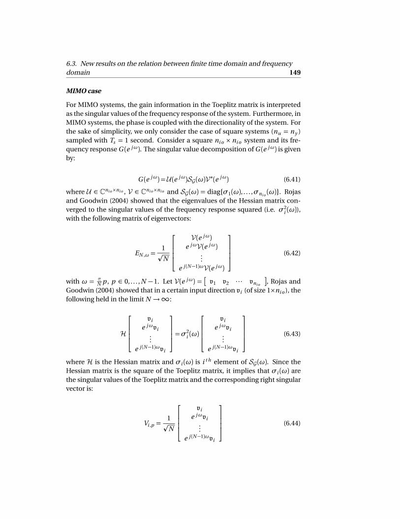
6.3. New results on the relation between finite time domain and frequencydomain 149
MIMO case
For MIMO systems, the gain information in the Toeplitz matrix is interpretedas the singular values of the frequency response of the system. Furthermore, inMIMO systems, the phase is coupled with the directionality of the system. Forthe sake of simplicity, we only consider the case of square systems (nu = ny )sampled with Ts = 1 second. Consider a square ni o × ni o system and its fre-quency response G (e jω). The singular value decomposition of G (e jω) is givenby:
G (e jω) =U (e jω)SG (ω)V∗(e jω) (6.41)
where U ∈ Cni o×ni o , V ∈ Cni o×ni o and SG (ω) = diagσ1(ω), . . . ,σni o(ω). Rojas
and Goodwin (2004) showed that the eigenvalues of the Hessian matrix con-verged to the singular values of the frequency response squared (i.e. σ2
i (ω)),with the following matrix of eigenvectors:
EN ,ω =1p
N
V(e jω)e jωV(e jω)
...e j (N−1)ωV(e jω)
(6.42)
with ω = πN p , p ∈ 0, . . . , N −1. Let V(e jω) =
v1 v2 · · · vni o
, Rojas andGoodwin (2004) showed that in a certain input direction vi (of size 1×ni o ), thefollowing held in the limit N →∞:
H
vi
e jωvi...
e j (N−1)ωvi
=σ2i (ω)
vi
e jωvi...
e j (N−1)ωvi
(6.43)
where H is the Hessian matrix and σi (ω) is i t h element of SG (ω). Since theHessian matrix is the square of the Toeplitz matrix, it implies that σi (ω) arethe singular values of the Toeplitz matrix and the corresponding right singularvector is:
Vi ,p =1p
N
vi
e jωvi...
e j (N−1)ωvi
(6.44)

150A fresh perspective on the connection between the frequency and finite time
domains
Since the vector above is complex and the Hessian and Toeplitz matrices arereal, we introduce their correct real singular vectors as follows. Let
vi =
Ai 1e jϕi 1
Ai 2e jϕi 2
...Ai 2ni o
e jϕi ni o
(6.45)
the real right singular values of the Toeplitz matrix are given by:
Vi ,p =
√
√ 2
N −1
Ai 1 cos(ϕi 1+ω)Ai 2 cos(ϕi 2+ω)
...Ai ni o
cos
ϕi ni o+ω
Ai 1 cos(ϕi 1+2ω)Ai 2 cos(ϕi 2+2ω)
...Ai ni o
cos
ϕi ni o+2ω
...
...Ai 1 cos
ϕi 1+Nω
Ai 2 cos
ϕi 2+Nω
...Ai ni o
cos
ϕi ni o+Nω
(6.46)
whereω= πN+1 p with p ∈ 1, . . . , N , which makesω vary from 0 toπwhen N is
long. The singular vectors Vi ,p now have two indices: i is the input direction as-sociated with column i of V(e jω) and p is the index of frequency π
N+1 p . Whenp varies from 1 to N and i from 1 to ni o , (6.46) generates N ni o right singularvectors, which is consistent with the size N ni o ×N ni o of the Toeplitz matrix.We now propose the following theorem that relates the phase and directionalinformation of the system with the singular vectors of the Toeplitz matrix.
Theorem 6.3.4 Consider a square system of size ni o × ni o and its frequencyresponse G (e jω). Its svd is given by
G (e jω) =U (e jω)SG (ω)V∗(e jω) (6.47)

6.3. New results on the relation between finite time domain and frequencydomain 151
withV(e jω) =
v1 v2 · · · vni o
andU (e jω) =
u1 u2 · · · uni o
.
As shown by Freudenberg and Looze (1988), the angle between singular sub-spaces (i.e. directional information) is defined as
φ(i ,ω) = arccos ||v∗i (ejω)ui (e
jω)|| (6.48)
and the phase difference between singular vectors is given by
∆θ (i ,ω) = arg(v∗i (ejω)ui (e
jω)) (6.49)
Consider the Toeplitz matrix T ∈N ni o ×N ni o with prediction horizon N
T =
M0 0 . . . . . . . . . 0...
......
...
Mk0. . . M0 0
...
0...
......
......
......
... 00 . . . 0 Mk0
. . . M0
(6.50)
Take the svd of T : T =U SV , with
V =
V1,1 V1,2 · · · V1,N · · · · · · Vni o ,1 Vni o ,2 · · · Vni o ,N
where Vi ,p is given in (6.46) and similarly
U =
U1,1 U1,2 · · · U1,N · · · · · · Uni o ,1 Uni o ,2 · · · Uni o ,N
S is a N ni o×N ni o diagonal matrix corresponding to the gains of the frequencyresponse. Then, in the limit N →∞, the following equality holds:
U >i ,p Vi ,p = cos
φ(i ,ω)
cos (∆θ (i ,ω)) (6.51)
withω= pN+1π, p ∈ 1, . . . , N , i ∈ 1, . . . , ni o .

152A fresh perspective on the connection between the frequency and finite time
domains
Proof. See Appendix C.From Theorem 6.3.4, equality (6.51) shows that the inner product of the left
and right singular vectors of the Toeplitz matrix in the time domain gives themultiplication of the directional angle and phase angle of the correspondingleft and right singular vectors of the frequency response in the frequency do-main. In the following, we discuss the relation between this product and thestability of the closed-loop system with a unity feedback and provides prelim-inary results.
Consider the same system with frequency response G (e jω)described above.The eigendecomposition of G (e jω) is given by:
G (e jω) =W∗(e jω)Λ(ω)W∗(e jω)−1
where Λ(ω)ni o×ni o is the diagonal matrix whose non-zero elements λi (ω) arethe eigenvalues of G (e jω) andW(e jω)ni o×ni o is the matrix of the correspondingeigenvectors:
W∗(e jω) =
w1 w2 . . .wni o
(6.52)
It is known that the stability of the closed-loop system with a unity feed-back is determined based on the locus of the eigenvalues λi (ω) over the fre-quency range [0;π]. For a stable open-loop system, the closed-loop system isstable if the characteristic loci of the eigenvalues do not encircle the point (-1;0)(Maciejowski (1989)). The closed-loop system is marginally stable if the locuscross the point (-1;0), i.e. there is some frequency where the eigenvalue is −1.Let λi (ω) be an arbitrary eigenvalue associated with its eigenvector wi (ω). Thesingular values and the pair of singular vectors of the frequency response at thecorresponding frequency are denotedσi (ω) and ui (ω),vi (ω), respectively.
In this analysis, symmetric open-loop transfer matrices are considered. Fora symmetric open-loop system, the SVD of G (e jω) coincides with the eigende-composition, i.e. the eigenvalue matrix Λ(ω) is also the singular value matrixS(ω) and the eigenvectors wi are equal to the singular vectors vi . Moreover,the SVD of the Toeplitz matrix gives the same information as the SVD of thefrequency response. Hence, the characteristic loci of the eigenvalues of G (e jω)can also be found in the SVD of the Toeplitz matrix.
Example Consider the following symmetric open-loop transfer matrix, whichis supposed to be the product of the controller and the process model in theLaplace domain:

6.3. New results on the relation between finite time domain and frequencydomain 153
−1 −0.5 0 0.5 1 1.5−1.5
−1
−0.5
0X: −0.6941Y: −0.0003162
Characteristic loci. High gain direction.
Real axis
Imag
inar
y ax
is
−0.4 −0.3 −0.2 −0.1 0 0.1 0.2 0.3 0.4 0.5−0.6
−0.4
−0.2
0
0.2
X: −0.2892Y: 0.0002765
Characteristic loci. Low gain direction.
Real axis
Imag
inar
y ax
is
Figure 6.13: Characteristic loci of the eigenvalues of the frequency response
1s 2+2s+1
1s+2
1s+2
1s+1
(6.53)
The system is discretised with a sampling period of 1 minute. The character-istic loci of Λ(ω) is given in Figure 6.13. The loci show that for each direction,the gain margins are 1/0.6941= 1.4407 and 1/0.2892= 3.4578, respectively. TheToeplitz matrix is constructed with a horizon of 200 samples. Figure 6.14 showsthat the inner product of the left and right singular vectors of the Toeplitz ma-trix coincide with that of the left and right singular vectors of the frequencyresponse over the frequency range [0,π]. The frequency where the inner prod-uct is -1 is also the critical point of the characteristic loci. It is shown in Figure6.15 that the same gain margins are obtained from the Toeplitz matrix for bothdirections (3.17 dB and 10.98 dB, respectively).
This analysis of the asymptotic behaviour of the Toeplitz matrix shows thatthe Toeplitz matrix contains the frequency-domain properties of the system.However, the use of this information in MPC design remains an open question.
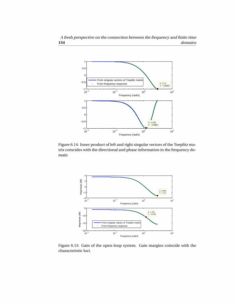
154A fresh perspective on the connection between the frequency and finite time
domains
10−2
10−1
100
101
−1
−0.5
0
0.5
1
X: 3.11Y: −0.9997
Frequency (rad/s)
10−2
10−1
100
101
−1
−0.5
0
0.5
1
X: 1.225Y: −0.9851
Frequency (rad/s)
From singular vectors of Toeplitz matrixFrom frequency response
Figure 6.14: Inner product of left and right singular vectors of the Toeplitz ma-trix coincides with the directional and phase information in the frequency do-main
10−2
10−1
100
101
−4
−2
0
2
4
X: 3.094Y: −3.17
Frequency (rad/s)
Mag
nitu
de (
dB)
10−2
10−1
100
101
−20
−15
−10
−5
X: 1.225Y: −10.98
Frequency (rad/s)
Mag
nitu
de (
dB)
From singular values of Toeplitz matrixFrom frequency response
Figure 6.15: Gain of the open-loop system. Gain margins coincide with thecharacteristic loci.

6.3. New results on the relation between finite time domain and frequencydomain 155
6.3.2 Finite-time properties of the Toeplitz and Hankel matrices
In the infinite time domain, there is a direct connection between the frequency-domain properties of the open-loop system and the Toeplitz matrix. Invertingthe matrix in the MPC solution gives a controller that is the inversion of the pro-cess. However, when one limits the number of singular values in the inversionup to a certain frequency, it does not lead to a controller that is the inversion ofthe process up to that exact frequency. The connection may be lost due to thereceding horizon principle of MPC. In this section, the finite-time propertiesof the Toeplitz and Hankel matrices are provided. The purpose of the analysisis to make a connection to their infinite-time properties.
Define matrix [H , T ] as the Toeplitz-Hankel matrix. The multiplication ofan arbitrary sine wave of any frequency and phase with the Toeplitz-Hankelmatrix gives an output sine wave of the same frequency. The relation betweenthe input and output sine waves provides the exact gain and phase of the open-loop system at the frequency of the sine waves.
Theorem 6.3.5 Consider the Toeplitz matrix T given in (6.4) and the Hankelmatrix H in (6.5) and a sine wave signal
x =
cos
−Np a s tω+ϕ
cos
−
Np a s t −1
ω+ϕ
...cosϕ
cos
ω+ϕ
cos
2ω+ϕ
...cos
Nω+ϕ
. (6.54)
This sine wave can be decomposed into the "past part" and the "future part"as follows:
xp a s t =
cos
−Np a s tω+ϕ
cos
−
Np a s t −1
ω+ϕ
...cosϕ
(6.55)
and

156A fresh perspective on the connection between the frequency and finite time
domains
x f u t u r e =
cos
ω+ϕ
cos
2ω+ϕ
...cos
Nω+ϕ
(6.56)
Letσω be the gain and φω be the phase of the open-loop system at frequencyω, the following holds for any φ, prediction horizon N , frequency ω and anNp a s t satisfying Np a s t > k0:
H xp a s t +T x f u t u r e =σω
cos
ω+ϕ+ϕω
cos
2ω+ϕ+ϕω
...cos
Nω+ϕ+ϕω
. (6.57)
Proof See Appendix C.This theorem shows the frequency-domain information is completely de-
termined by the Toeplitz and Hankel matrices. This is not surprising since thematrices are built from the FIR model of the system. Based on this theorem, thefollowing corollary shows how to construct an orthogonal matrix consisting ofsine waves that is similar to the singular vector matrix of the Toeplitz matrix.This corollary is put forward in order to investigate the change from infinitehorizon to finite horizon.
Corollary 6.3.6 Given the following matrices:
Xp a s t =
xp a s t1 x
p a s t2 · · · x
p a s tN
(6.58)
where
xp a s ti =
cos
−Np a s tωi +π2 −ϕωi
cos
−
Np a s t −1
ωi +π2 −ϕωi
...cos
π2 −ϕωi
(6.59)
for 1≤ i ≤N andωi =πi
N+1 ;

6.3. New results on the relation between finite time domain and frequencydomain 157
X f u t u r e =
xf u t u r e
1 xf u t u r e
2 · · · xf u t u r e
N
(6.60)
where
xf u t u r e
i =
cos
ωi +π2 −ϕωi
cos
2ωi +π2 −ϕωi
...cos
Nωi +π2 −ϕωi
(6.61)
and
Yf u t u r e =
yf u t u r e
1 yf u t u r e
2 · · · yf u t u r e
N
(6.62)
where
yf u t u r e
i =
cos
ωi +π2
cos
2ωi +π2
...cos
Nωi +π2
(6.63)
it follows that
H T
Xp a s t
X f u t u r e
= Yf u t u r e
σω10 · · · 0
0 σω2
......
......
... 00 · · · 0 σωN
. (6.64)
Expression (6.64) can be considered as a decomposition of matrix
H T
.The difference between this decomposition and the SVD is that matrix Yf u t u r e
is orthogonal while matrix X f u t u r e is not.
Theorem 6.3.7 Matrix Yf u t u r e constructed in Corollary 6.3.6 is orthogonal and
the lengths of the vectors yf u t u r e
i are the same for 1≤ i ≤N .

158A fresh perspective on the connection between the frequency and finite time
domains
Proof See Appendix C.Theorem 6.3.7 shows that matrix Yf u t u r e in decomposition (6.64) can be
made orthonormal by dividing the matrix by the length of yf u t u r e
i . Due to thefact that the construction of matrix X f u t u r e depends on the phase of the open-loop system atωi , there is no guarantee that X f u t u r e is orthonormal. However,when N →∞, the sine waves tend to be orthogonal to each other and thereforematrix X f u t u r e tends to be orthonormal. This can be considered as a majordifference between the infinite time domain and the finite time domain.
6.3.3 Open issue: Relation between SVD and frequency-domain prop-erties in finite-time domain
In this subsection, the relation between the SVD of the Toeplitz-Hankel matrixand decomposition (6.64) is investigated. The aim of this analysis is to linkthe SVD to the frequency-domain properties of the system when the horizonis finite. This analysis is further development of that in Ludlage (1997). Due tothe shortage of available time, the analysis is limited and follow-up questionsare then posed.
Consider a system of order n . The SVD of the Toeplitz-Hankel matrix isgiven by:
H T
=UH T
ΣH T 0
V >H T 11 V >H T 21V >H T 12 V >H T 22
(6.65)
and:
H =UH TΣH T V >H T 11
T =UH TΣH T V >H T 21.(6.66)
Thanks to the properties of SVD, matrices UH T and
VH T 11 VH T 12
VH T 21 VH T 22
are both
orthonormal. As shown in Subsection 6.3.2, matrix Yf u t u r e in decomposition(6.64) can be orthonormal while matrix X f u t u r e is not orthonormal. There-
fore, the relation between matrix
Xp a s t
X f u t u r e
and matrix
VH T 11 VH T 12
VH T 21 VH T 22
is
investigated to connect the frequency-domain information of the system andthe SVD of the Toeplitz-Hankel matrix when the horizon is finite.
Since the order of the system is n , the rank of the Hankel matrix is n . Hence,the SVD of matrix V >H T 11 is given by:

6.3. New results on the relation between finite time domain and frequencydomain 159
V >H T 11 = U
Σ11 00 0
V > (6.67)
where Σ11 ∈Rn×n . In addition, due to the orthonormality of
VH T 11 VH T 12
VH T 21 VH T 22
,
it follows that:
V >H T 11VH T 11+V >H T 21VH T 21 = I
⇒ U
Σ211 00 0
U >+V >H T 21VH T 21 = I
⇒
Σ211 00 0
+U >V >H T 21VH T 21U = I
⇒ U >V >H T 21VH T 21U =
I − Σ211 0
0 I
⇒V >H T 21VH T 21 = U
I − Σ211 0
0 I
U >.
(6.68)
Therefore, the SVD of V >H T 21 is given by
V >H T 21 = U
q
I − Σ211 0
0 I
V > (6.69)
and matrix
VH T 11 VH T 12
VH T 21 VH T 22
can be written as follows:
VH T 11 VH T 12
VH T 21 VH T 22
=
V 00 V
Σ11 0q
I − Σ211 0
0 0 0 Iq
I − Σ211 0 −Σ11 0
0 I 0 0
U > 00 U >
.
(6.70)
Let
α1
α2
=
VH T 11 VH T 12
VH T 21 VH T 22
> Xp a s t
X f u t u r e
(6.71)
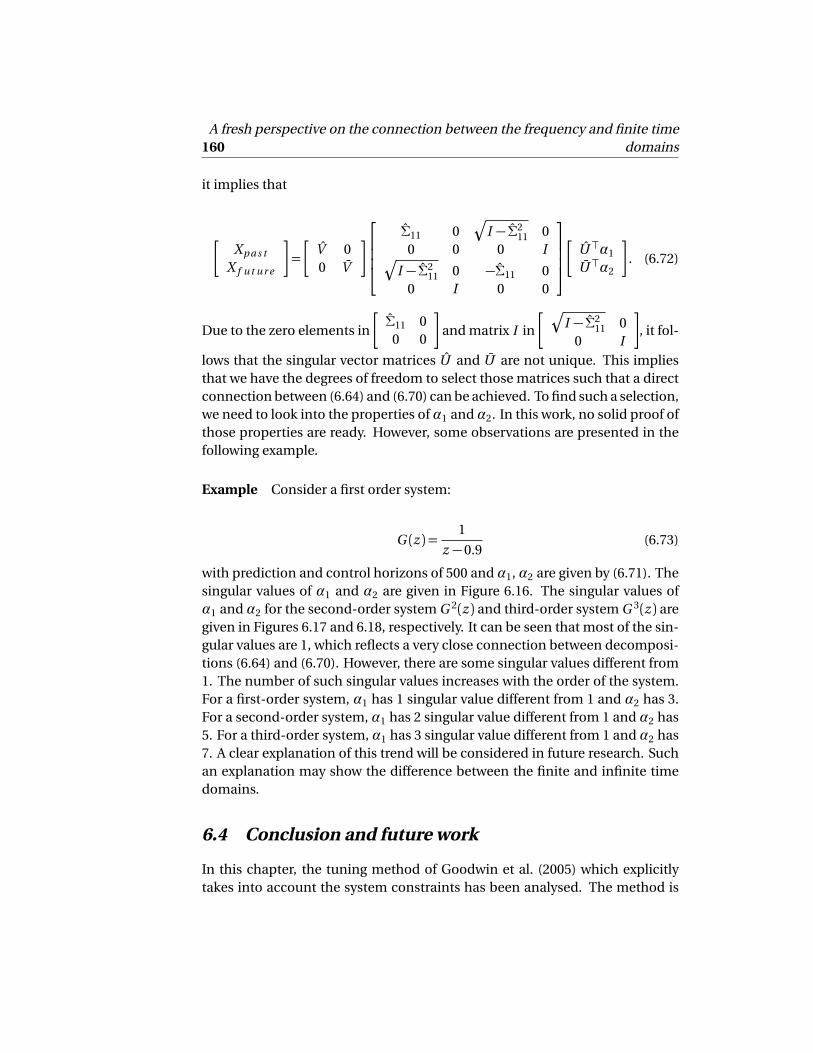
160A fresh perspective on the connection between the frequency and finite time
domains
it implies that
Xp a s t
X f u t u r e
=
V 00 V
Σ11 0q
I − Σ211 0
0 0 0 Iq
I − Σ211 0 −Σ11 0
0 I 0 0
U >α1
U >α2
. (6.72)
Due to the zero elements in
Σ11 00 0
and matrix I in
q
I − Σ211 0
0 I
, it fol-
lows that the singular vector matrices U and U are not unique. This impliesthat we have the degrees of freedom to select those matrices such that a directconnection between (6.64) and (6.70) can be achieved. To find such a selection,we need to look into the properties of α1 and α2. In this work, no solid proof ofthose properties are ready. However, some observations are presented in thefollowing example.
Example Consider a first order system:
G (z ) =1
z −0.9(6.73)
with prediction and control horizons of 500 and α1, α2 are given by (6.71). Thesingular values of α1 and α2 are given in Figure 6.16. The singular values ofα1 and α2 for the second-order system G 2(z ) and third-order system G 3(z ) aregiven in Figures 6.17 and 6.18, respectively. It can be seen that most of the sin-gular values are 1, which reflects a very close connection between decomposi-tions (6.64) and (6.70). However, there are some singular values different from1. The number of such singular values increases with the order of the system.For a first-order system, α1 has 1 singular value different from 1 and α2 has 3.For a second-order system, α1 has 2 singular value different from 1 and α2 has5. For a third-order system, α1 has 3 singular value different from 1 and α2 has7. A clear explanation of this trend will be considered in future research. Suchan explanation may show the difference between the finite and infinite timedomains.
6.4 Conclusion and future work
In this chapter, the tuning method of Goodwin et al. (2005) which explicitlytakes into account the system constraints has been analysed. The method is

6.4. Conclusion and future work 161
0 100 200 300 400 5000
0.5
1
1.5
Singular values of α1
0 100 200 300 400 5000
0.5
1
1.5
Singular values of α2
Figure 6.16: Singular values of α1 and α2 for a first-order system.
0 100 200 300 400 5000
0.5
1
1.5
Singular values of α1
0 100 200 300 400 5000
0.5
1
1.5
Singular values of α2
Figure 6.17: Singular values of α1 and α2 for a second-order system.

162A fresh perspective on the connection between the frequency and finite time
domains
0 100 200 300 400 5000
0.5
1
1.5
Singular values of α1
0 100 200 300 400 5000
0.5
1
1.5
Singular values of α2
Figure 6.18: Singular values of α1 and α2 for a third-order system.
based on limiting the number of non-zero singular values of the Toeplitz matrixwhen calculating the MPC solution. It is shown that the closed-loop bandwidthof the controller is reduced when fewer singular values are inverted. However,the direct connection between the singular values and the frequency-domainproperties of the system is still missing.
Therefore, this chapter further investigates the finite-time and asymptoticbehaviour of the Toeplitz matrix. It is shown that the frequency-domain infor-mation of the open-loop system can be found in the SVD of the Toeplitz ma-trix. Rojas et al. (2003, 2004) and Rojas and Goodwin (2004) showed that theeigenvalues of the Hessian matrix asymptotically converge to the energy den-sity spectrum. We extended that work and showed the relation between thesingular vectors of the Toeplitz matrix and the phase and directional informa-tion of the associated system.
Singular vectors (6.35) are sine-wave signals of a unique frequency. Never-theless, in the case of resonant systems, there exist degenerate singular values,and the SVD of the Toeplitz matrix is not unique any more, since a normalisedlinear combination of the corresponding singular vectors also provides newsingular vectors. This leads to the fact that a singular vector can contain morethan one frequency, due to that type of combination of the sine waves. In thiscase, filtering and separating the different frequency parts can enable us to re-

6.4. Conclusion and future work 163
tain the original singular vectors (6.35), which contain only one frequency. Thiscase will be further investigated in the future.
It is shown that the singular values and vectors of the Toeplitz matrix con-tain the gain and phase information of the open-loop system over the frequencyrange [0;π]. This frequency range is divided into N frequency points nπ
N+1 forn = 1; 2; . . . ; N . When N →∞, the frequency points approach a continuousfrequency range and the full Bode plot can be found in the SVD of the Toeplitzmatrix. Decreasing N will reduce the resolution of the gain and phase informa-tion in the singular values and singular vectors but the frequency range [0;π]remains unchanged. The inverse of the Toeplitz matrix in the MPC solution isequivalent to the inverse of the open-loop system in the IMC controller. How-ever, when some of the singular values of the Toeplitz matrix are set to 0, thesimilar effect on the frequency-domain properties of the IMC controller can-not be found. This can be attributed to the receding horizon principle of MPCin the finite time domain. When N is finite, decomposition (6.64) is close toan SVD and contains the gain and phase information of the open-loop system.However, the orthonormality of one singular vector matrix is lost. This is dueto the fact that sine waves tend to be orthogonal to each other in the infinitetime domain but not in the finite time domain.
Future research can therefore focus on the finite-time-domain behaviourof the Toeplitz and Hankel matrices, by further analysing the relation betweendecomposition (6.64) and the SVD of the Toeplitz matrix. Despite the asymp-totic connection between the SVD of the Toeplitz matrix and the frequency-domain characteristics of the system, the effect of the receding horizon con-troller on this connection is still an open question. Although changing the sin-gular value matrix is equivalent to changing the input weight R , how to usethe connection described in this chapter in tuning MPC is still under investi-gation. In the future, an SVD-based tuning method that allows us to adjust thefrequency-domain specifications of MPC while respecting constraints will beinvestigated.

164A fresh perspective on the connection between the frequency and finite time
domains

7Industrial validation: FT-depropaniser
7.1 Introduction7.2 The FT-depropaniser7.3 Controller tuning for the
FT-depropaniser simulator
7.4 Controller tuning for theactual FT-depropaniser
7.5 Conclusion
7.1 Introduction
This chapter presents the implementation of the practical tuning method in-troduced in Chapter 3 on an industrial process: the FT depropaniser of SASOLLimited. Based on the frequency-domain characteristics of the process, themanual seeking is used to find the optimal closed-loop bandwidth for the sys-tem. The experiments are firstly performed on a simulator of the FT-depropaniser,which is built for training operators and duplicates the dynamics of the actualprocess. After an analysis of the result on the simulator, the experiments areconducted on the actual plant.
On the simulator, the first stage of the experiments is identifying a modelof the open-loop system using step tests and RBS tests. The second stage ofthe experiments is to commission an MPC and find the optimal closed-loopbandwidth using the practical tuning method presented in Chapter 3. Next,a fictitious change in the dynamics of the simulator system is made by mod-ifying the dynamics of the identified model. In other words, the model-plantmismatch is caused by keeping the plant dynamics unchanged while altering

166 Industrial validation: FT-depropaniser
the MPC model. The tuning method then shows the new optimal closed-loopbandwidth in the presence of modelling errors.
On the actual plant, the identification is performed using RBS test signalswhose characteristics are chosen based on the identification of the simulatorprocess. Due to the limit on the amount of time allowed for experiments, steptests and staircase tests are not carried out on the plant. However, since thesimulator was built to duplicate the dynamics of the actual plant, the modelof the simulator process and the excitation signals used to identify it enable usto design suitable RBS test signals for the actual plant without performing steptests and staircase tests. The experiments after the identification are similar towhat is performed on the simulator. Specific differences between the tests onthe simulator and on the plant are given in the corresponding sections.
The rest of the chapter is organised as follows. Section 7.2 provides an intro-duction to the FT-depropaniser and the associated base-layer control as wellas APC systems. Details of the experiments on the simulator are given in Sec-tion 7.3 and those on the actual plant in Section 7.4. Section 7.5 concludes thechapter.
7.2 The FT-depropaniser
Figure 7.1: FT-depropaniser in the SCC unit. Photo courtesy of Sasol.

7.2. The FT-depropaniser 167
This introduction to the FT-depropaniser is mainly based on Sasol (2014),Kotze et al. (2011) and Pieterse et al. (2011). The FT-depropaniser (Figure 7.1)is part of the Sasol Synthetic fuels refinery in Secunda, South Africa. The oper-ation of Sasol Synfuels involves receiving coal from five mines in Mpumalanga,South Africa. The coal is then crushed and blended so as to produce an evenquality distribution. Gasification of the obtained coal is performed at a temper-ature of 1300 degrees Celsius. The product of the gasification process producescomponents for making synthetic fuels and other downstream chemicals. InSasol Synfuels, the SCC unit is used to convert high-boiling, high-molecularweight hydrocarbon fractions of petroleum crude oils to more valuable gaso-line, olefinic gases, and other products, similar to a refinery FCC unit (Gary andHandwerk (2001)). Low molecular weight olefins and paraffins are convertedto ethylene (C2H4) and propylene (C3H6) in a dilute phase reactor-riser.
Located in the cold side of the SCC unit, the FT-depropaniser separates C3’sand lighter components from C4’s and heavier components in the feed stream.C3’s hydrocarbons consist of propane (C3H8), propylene (C3H6), etc and C4’sconsist of n-butane, isobutane (C4H10), butylene (C4H8), etc. Since volatil-ity decreases when molecular weight increases, the considerable difference inmolecular weight between C3’s and C4’s makes the separation between thempossible with a 56-tray FT-depropaniser. The separation between, for exam-ple, propane (C3H8) and propylene (C3H6) requires a much taller distillationcolumn.
7.2.1 Process and control structure description
A schematic overview of the FT-depropaniser system is given in Figure 7.2. Acircle with the text "SP" inside denotes a PID controller. The set-point of a PIDcontroller can be set by the cascade control, the MPC, or the operators. Thedashed lines denote the feedback of the PID controllers and the solid lines arethe cascade connection or the connection to the valves.
There are 4 upstream feeds from 4 upstream units (U23, U223, U70, U285)entering the system. Possible lighter components in the feed stream includemethane (C H4), ethane (C2H6), ethylene (C2H4), water (H2O ) and methanol(C H3O H ). The heavier components are the heavy hydrocarbons: C5’s, C6’sand C7’s. The upstream feeds enter a feed surge drum and the stream from thefeed surge drum can be routed to the following systems:
• The FT-depropaniser column,
• The Cat Poly C3 rich liquid return header.

168 Industrial validation: FT-depropaniser
Liquid
Vapour
TRAY 56
TRAY 39 (side draw)
TRAY 34
BUFFER
TRAY 1
Feed Surge Drum
U23
U223
U70
U285
CatPoly C3
SP3
purge gas
MV4
MV3
MV2
Condenser +Reflux drum
purge gas
total reflux
LiquidDryer
C3Splitter
Reboiler
Water Cooler CatPoly C4
MV1
SP2
SP6
ratio control
SP8Δpressure
control
cut handle
fractionation handle
TRAY 19SP1
SP7
SP5
SP4
Figure 7.2: Schematic overview of the FT-depropaniser system.
The FT-depropaniser is a 56-tray tower with total reflux, which includes aside draw section on tray 39. The contents of the feed surge drum are sent tothe FT-depropaniser column at tray 34. For the FT-depropaniser column, it isvery important to maintain a stable feed flow. The use of the feed surge drumallows the feed to the column to be manipulated by the MPC or the operators.This prevents oscillations in the upstream feed from transmitting themselvesto the feed to the column. The side draw stream from the FT-depropaniser,which contains mainly C3’s and lighter components, is directed to a liquid drierto remove water and methanol before entering the C3 splitter. The liquid drierensures the water specification of the FT-depropaniser’s product. The C3 split-ter separates Propane (C3H8) and Propylene (C3H6). The bottom product ofthe FT-depropaniser, which consists of C4’s and heavier components, is cooledagainst tempered water in the cooler before going to the Cat Poly C4 rich liquidheader. In addition, a vapour side draw from the FT-depropaniser is taken ontray 19, which provides pressurising gas for the feed surge drum. This controlsthe flow and maintains the pressure in the drum.
7.2. The FT-depropaniser 169
7.2.2 Base-layer control
• Feed drum level: Cascade control is used to keep the feed drum level at itsset-point if this is not part of the MPC. The PID controller SP 1 takes thefeed drum level value and sends the set-point value to the PID controllerSP 2, which manipulates the flow from the feed surge drum to the CatPoly C3. This cascade connection will be broken if the feed drum level ispart of the MPC and the flow from the feed drum to the Cat Poly C3 is amanipulated variable of the MPC. The set-point of the feed drum level isprovided by operators if not given by the MPC.
• Feed flow: SP 3 controls the feed flow from the feed drum to the FT-depropaniser. This PID may receive the set-point from the MPC sincethe use of the feed surge drum allows the feed flow to the column to bemanipulated by the MPC. However, in some cases, operators prefer tohave access to the set-point of this PID to manipulate the feed flow. Inthis case, the priority is given to operators and the feed flow becomes ameasurable disturbance of the MPC.
• Feed drum pressure: SP 4 manipulates the vapour flow from tray 19 ofthe FT-depropaniser column to the feed drum in order to control the feeddrum pressure. The set-point of this PID is given by operators.
• Side draw flow: SP 5 controls the side draw to feed ratio and receives theset-point from the MPC. It computes the set-point for SP 6, which con-trols the side draw flow and is cascaded to SP 5.
• Delta pressure control: SP 7 controls the differential pressure betweenthe top and bottom of the column, and receives the set-point from theMPC. It is cascaded to SP 8, which controls the reboiler flow.
7.2.3 APC
The control objectives of the MPC are:
• Maximise the production rate by increasing the feed (when possible) andthe side draw flow.
• Maintain the product specification. It is reflected in the amount of C4’sin the side draw.
• Prevent flooding in the feed drum by manipulating the feed flow to theCat Poly C3 header.

170 Industrial validation: FT-depropaniser
• Prevent flooding in the column by imposing an upper limit on the differ-ential pressure.
• Prevent flaring by imposing an upper limit on the column pressure.
• Prevent sudden and dramatic breakthrough of C4’s by imposing an upperlimit on the bottom temperature.
The 11 controlled variables (CV) of the MPC and their limits are given inTable 7.1, where "OP" means valve opening percentage. The depropaniser has4 manipulated variables (MV’s), which are given in Table 7.2. The maximummoves of the MV’s are given in Table 7.3.
Table 7.1: Controlled outputs of the FT-depropaniser and their limits
Variable Low limit High limit Unit
CV1 C4 Content in the side draw N/A 2000 PPMCV2 Feed Drum Level 40 77 %CV3 Feed Drum Level Rate of Change N/A N/A %CV4 Column Pressure 1170 1400 kPaCV5 Bottom Temperature N/A 90 CCV6 Feed Flow OP 1 99 %CV7 Side-draw Flow OP 1 99 %CV8 Reboil 0 14 ∗
CV9 Reboil Flow OP 1 99 %CV10 Reflux Flow OP 1 99 %CV11 Feed to C3 Header OP 1 99 %
Table 7.2: Manipulated variables of the FT-depropaniser and their limits
Variable Low limit High limit Unit
MV1 Column feed flow 45 65 ∗
MV2 Side-draw Flow to Feed Ratio 45 70 %MV3 Column differential pressure 30 39 kPaMV4 Feed to C3 Header .1 70 ∗
∗Not shown for confidentiality reasons.

7.2. The FT-depropaniser 171
Table 7.3: Maximum moves of the manipulated variables of the FT-depropaniser
Variable Max move down Max move up
MV1 Column feed flow .3 .3MV2 Side-draw Flow to Feed Ratio 0.5 0.25MV3 Column differential pressure 0.2 0.2MV4 Feed to C3 Header 5 5
According to the control objectives, the key CV’s of the MPC are the C4’scontent in the side draw (CV1), the feed drum level (CV2), the column pres-sure (CV4) and the bottom temperature (CV5). In the experiments conducted,only CV1 is steered to its set-point to maintain product specification, while theother CV’s are kept within the limits. Therefore, the feed drum level (CV2) iscontrolled by a cascade loop (SP 1 and SP 2 in Figure 7.2) and MV4 is droppedout of the MPC and considered as a measurable disturbance in the MPC model.The use of the column feed flow (MV1) in controlling the C4’s content is un-wanted since a stable feed flow is desired. Hence, the only purpose of MV1 inthe MPC is to avoid flooding in the feed drum. If an unusual dramatic jumpin the upstream feed occurs, the set-point of the feed flow can be increased todrain the feed drum. On the other hand, if the upstream feed reduces dras-tically and the flow to the Cat Poly C3 header is saturated, a decrease in theset-point of the column feed flow is needed to avoid emptying the feed drum.Nevertheless, these are undesired critical cases and the column feed flow isgenerally kept stable. Hence, the variables used to control the distillation areprimarily the side draw flow to feed ratio (MV2) and the pressure difference be-tween the top and the bottom of the column (MV3). In addition, MV2 is alsoused for the maximisation of production rate.
The effect of MV2 and MV3 on the composition profile of the column isgiven in Figure 7.3. Note that Figure 7.3 was not built from actual data of theFT-depropaniser and only serves as an illustration. In this configuration, MV2is considered as the cut handle and MV3 as the fractionation handle of the col-umn. If the side draw to feed ratio (MV2) is increased while MV3 is kept con-stant, the quality of the top product goes down while that of the bottom prod-uct becomes better. This is reflected by the fact that the C4’s content in theside draw rises with the increase of MV2. If the differential pressure (MV3) isincreased while MV2 is kept constant, the quality of both top and bottom prod-ucts becomes better. Maximising MV2 and using MV3 for controlling the qual-

172 Industrial validation: FT-depropaniser
ity is therefore equivalent to controlling the composition of both top and bot-tom products. Hence, this control scheme is similar to the DV-configuration(Skogestad (1997)).
0 10 20 30 40 50 600
0.1
0.2
0.3
0.4
0.5
0.6
0.7
0.8
0.9
1
Stage number
Mol
e fr
actio
n
Composition profile of the light component (C3’s) in the column
NominalEffect of MV2 (cut handle)Effect of MV3 (fractionation handle)
Figure 7.3: Effect of increasing MV2 (cut handle) and MV3 (fractionation han-dle) on composition profile of light component (C3’s).
7.3 Controller tuning for the FT-depropaniser simulator
7.3.1 Initial settings
The experiments are first performed on a simulator of the FT-depropaniser,which is developed to train operators. Built on Honeywell’s UniSim OperationsSuite, the simulator was constructed to realistically and accurately reproducethe process dynamics that characterise the actual FT-depropaniser. The op-erating range of the simulator is also chosen to closely reproduce the normaloperation of the actual plant. The operating point considered in this experi-ment is given in Table 7.4. The behaviour of several important outputs (namely

7.3. Controller tuning for the FT-depropaniser simulator 173
the C4 content in the side draw, the level of the feed surge drum, the columnpressure and the bottom temperature) at steady state is given in Figure 7.4.
Table 7.4: Operating point of the simulator
Feed flow (MV1) 55Side-draw flow to feed ratio (MV2) 47
Column differential pressure (MV3) 32.78
0 2 4 6 8150
200
250
300
350
C4 content in the side draw at steady state
Time (hours)
PP
M
0 2 4 6 8
49.95
50
50.05
50.1
50.15
50.2Level of feed surge drum at steady state
Time (hours)
%
0 2 4 6 81260
1280
1300
1320Column pressure at steady state
Time (hours)
kPa
0 2 4 6 878
80
82
84
86Bottom temperature at steady state
Time (hours)
Cel
sius
Figure 7.4: Major CV’s of the simulator at steady state.
CV3, the feed drum level rate of change, is not of interest and dropped outof the system. CV7, the side-draw flow OP is also dropped due to technicalcommunication problems. Hence, the simulator system has 9 CV’s instead ofthe original 11 CV’s. A control scheme of the simulator is given in Figure 7.5.Furthermore, instead of the actual values of the C4’s content, its logarithm isused as CV1, the key controlled output in the model. The steady-state valuesof the CV’s used for open-loop identification are obtained from the mean of the

174 Industrial validation: FT-depropaniser
steady-state signals. These values are given in Table 7.5.
APC PID
Process
MV2 (SP)
MV3 (SP)
MV4 = DV
CV1 to CV11 with CV3 and CV7 dropped.
Valve closure percentage
MV1 (SP)
Figure 7.5: Schematic overview of the control system of the simulator. The PIDblock only includes the PID controllers of MV1, MV2, MV3 and MV4.
Table 7.5: Steady state values of the simulator variables
Variable SS values Unit
CV1 Logarithm of C4 Content in the side draw 5.4346 PPMCV2 Feed Drum Level 50 %CV4 Column Pressure 1302.4 kPaCV5 Bottom Temperature 81.96 CCV6 Feed Flow OP 58.0 %CV8 Reboil 10.477 ∗
CV9 Reboil Flow OP 89.6 %CV10 Reflux Flow OP 63.0 %CV11 Feed to C3 Header OP 3.19 %
∗Not shown for confidentiality reasons.

7.3. Controller tuning for the FT-depropaniser simulator 175
7.3.2 Model
A linear model of the FT-depropaniser simulator is identified around the con-sidered operating point using step test signals and RBS (Guidi et al. (2013)). Thetransfer functions from MV2 and MV3 to CV1 are given by:
Table 7.6: Major transfer functions of the simulator process.
From MV2 From MV3
To CV1 −0.006275z−1+0.01187z−2
1−1.756z−1+0.7803z−20.2742z−1−0.2889z−2
1−1.756z−1+0.7803z−2
The step response from the major MV’s (MV2 and MV3) to the key CV (CV1) isgiven in Figure 7.6. It shows a positive gain from MV2 to CV1, which shows thatthe more product is drawn from the side draw, the higher the C4’s content inthe side draw. The change in MV2, the side draw to feed ratio, results in a movein the cut of the column. The model also shows a negative gain with inverseresponse from MV3 to CV1, which means that a greater difference between thetop and bottom pressure leads to better separation of the components.
0 0.5 1 1.5 2−0.8
−0.6
−0.4
−0.2
0
0.2
0.4
0.6
0.8From: In(1)
0 0.5 1 1.5 2
From: In(2)
Step Response
Time (hours)
Am
plitu
de (
PP
M)
Figure 7.6: Step response from MV2 and MV3 to CV1 of the simulator model.

176 Industrial validation: FT-depropaniser
7.3.3 Tuning at commissioning
A set-point of 229.2 PPM (namely 5.4346 for log(CV1)), which is also the meanvalue of the C4’s in the side draw at steady state, is selected for the C4’s contentin the side draw to ensure the quality of the product. Therefore, the focus ofthe control system is to reject disturbances affecting the product quality. Tomaximise the production rate, the side draw to feed ratio (MV2) is steered to itsset-point of 69.5 %, which is close to its upper limit of 70 %. Although the feedrate (MV1) can be manipulated thanks to the use of the feed surge drum, fluctu-ation in this variable is not desired and therefore a set-point of 55 is used for thefeed rate. The use of MV1 will be active if and only if the level of the feed surgedrum (CV2) is higher than 65%, in order to avoid flooding in the drum. Thehorizons are chosen to cover the dominant dynamics of the open-loop systemtaking into consideration the computational capacity of the closed-loop iden-tification method in future experiments (Larsson et al. (2013)). Based on theseconfigurations and the dynamics of the open-loop system, the following initialtuning parameters are proposed:
• Control horizon: 10 samples.
• Prediction horizon: 50 samples (namely 100 minutes).
• Penalty weights on CV’s : [qy 0 0 0 0 0 0 0 0] since only the C4 content iscontrolled at its set-point.
• Penalty weights on changes of MV’s: [25 1 1]. Significant variation in thefeed rate (MV1) is not desired. Hence, a high penalty weight is put onthe changes of the feed rate (MV1). A weighting factor of 1 is used on thechanges of side draw ratio (MV2) and the weight on the changes of thedelta pressure (MV3) is 1.
• Penalty weights on MV’s: [5 2e-5 0]. A high weight of 5 is put on the de-viation of the feed rate from its set-point to avoid using the feed in con-trolling the C4 content. The side draw ratio’s (MV2’s) set-point is 69.5 %,which is close to its upper limit of 70 %. This setting maximises the pro-duction rate. However, in this experiment, the variance of the C4 contentis the main focus of the tuning. Therefore, a low weight of 2e-5 is put onthe deviation of the side draw ratio (MV2) from 69.5 %.
The cost function of the MPC is then given by:
J (k ) =50∑
i=1
qy
y (k + i )−229.22
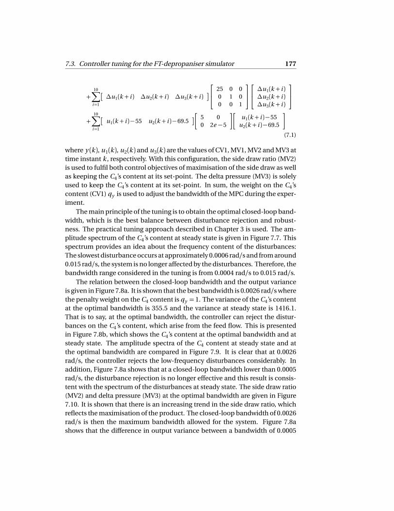
7.3. Controller tuning for the FT-depropaniser simulator 177
+10∑
i=1
∆u1(k + i ) ∆u2(k + i ) ∆u3(k + i )
25 0 00 1 00 0 1
∆u1(k + i )∆u2(k + i )∆u3(k + i )
+10∑
i=1
u1(k + i )−55 u2(k + i )−69.5
5 00 2e −5
u1(k + i )−55u2(k + i )−69.5
(7.1)
where y (k ), u1(k ), u2(k ) and u3(k ) are the values of CV1, MV1, MV2 and MV3 attime instant k , respectively. With this configuration, the side draw ratio (MV2)is used to fulfil both control objectives of maximisation of the side draw as wellas keeping the C4’s content at its set-point. The delta pressure (MV3) is solelyused to keep the C4’s content at its set-point. In sum, the weight on the C4’scontent (CV1) qy is used to adjust the bandwidth of the MPC during the exper-iment.
The main principle of the tuning is to obtain the optimal closed-loop band-width, which is the best balance between disturbance rejection and robust-ness. The practical tuning approach described in Chapter 3 is used. The am-plitude spectrum of the C4’s content at steady state is given in Figure 7.7. Thisspectrum provides an idea about the frequency content of the disturbances:The slowest disturbance occurs at approximately 0.0006 rad/s and from around0.015 rad/s, the system is no longer affected by the disturbances. Therefore, thebandwidth range considered in the tuning is from 0.0004 rad/s to 0.015 rad/s.
The relation between the closed-loop bandwidth and the output varianceis given in Figure 7.8a. It is shown that the best bandwidth is 0.0026 rad/s wherethe penalty weight on the C4 content is qy = 1. The variance of the C4’s contentat the optimal bandwidth is 355.5 and the variance at steady state is 1416.1.That is to say, at the optimal bandwidth, the controller can reject the distur-bances on the C4’s content, which arise from the feed flow. This is presentedin Figure 7.8b, which shows the C4’s content at the optimal bandwidth and atsteady state. The amplitude spectra of the C4 content at steady state and atthe optimal bandwidth are compared in Figure 7.9. It is clear that at 0.0026rad/s, the controller rejects the low-frequency disturbances considerably. Inaddition, Figure 7.8a shows that at a closed-loop bandwidth lower than 0.0005rad/s, the disturbance rejection is no longer effective and this result is consis-tent with the spectrum of the disturbances at steady state. The side draw ratio(MV2) and delta pressure (MV3) at the optimal bandwidth are given in Figure7.10. It is shown that there is an increasing trend in the side draw ratio, whichreflects the maximisation of the product. The closed-loop bandwidth of 0.0026rad/s is then the maximum bandwidth allowed for the system. Figure 7.8ashows that the difference in output variance between a bandwidth of 0.0005

178 Industrial validation: FT-depropaniser
0.005 0.01 0.015 0.02 0.025 0.03 0.035 0.040
5
10
15
20
25
30
35X: 0.0006136Y: 37.95
Single−Sided Amplitude Spectrum of C4 content
Frequency (rad/s)
X: 0.001227Y: 29.95
Figure 7.7: Amplitude spectrum of the C4’s content at steady state.
and 0.0026 is not too high, compared to the extremes of the curve. Therefore,in reality, a closed-loop bandwidth lower than 0.0026 should be chosen for thesystem in order to obtain more robustness. Nonetheless, in these experiments,the closed-loop bandwidth of 0.0026 rad/s is chosen for commissioning sincethis maximum bandwidth allowed is more likely to give a performance dropdue to a change in the plant dynamics.
0 0.5 1 1.5 2 2.5 3
x 10−3
0
500
1000
1500
2000
2500
3000
3500
4000
4500
5000
X: 0.0026Y: 355.5
Closed−loop bandwidth [rad/s]
Var
ianc
e of
C4
cont
ent
(a) Relation between closed-loop band-width and variance of C4 content.
0 1 2 3 4 5 6 7 8160
180
200
220
240
260
280
300
320
340C4 content in the side draw
Time (hours)
PP
M
In closed loopIn open loopSet−point
(b) C4 content in the side draw at optimalbandwidth.
Figure 7.8: Results of the tuning in commissioning phase.

7.3. Controller tuning for the FT-depropaniser simulator 179
0.005 0.01 0.015 0.02 0.025 0.03 0.035 0.040
5
10
15
20
25
30
35
X: 0.001227Y: 29.95
Single−Sided Amplitude Spectrum of C4 content
Frequency (rad/s)
X: 0.0006136Y: 37.95
Figure 7.9: Amplitude spectra of the C4’s content.
7.3.4 Tuning for performance maintenance
Performance drop
In the second tuning experiment, the poles of the model are changed in orderto cause a degradation in the closed-loop performance:
pd e g r a d e d = 0.98po l d (7.2)
where pd e g r a d e d are the poles of the degraded model and po l d are the poles ofthe initial model. With this degraded model, the variance of the C4 content inthe side draw goes from 355.5 to 1398. The C4 content in the two cases is givenin Figure 7.11. It is obvious that the performance with the degraded model isworse than the commissioned performance. The closed-loop system is thenre-tuned so as to retain the performance.
Re-tuning
In the re-tuning, the bandwidth of the MPC is reduced to retain the closed-loopperformance. The new bandwidth-variance relation is given in Figure 7.12a.Due to more significant model-plant mismatch, the new optimal bandwidth is

180 Industrial validation: FT-depropaniser
0 1 2 3 4 5 6 7 844
46
48
50
Time (hours)
%
Side draw to feed ratio and its linear trend
y = 0.037*x + 47
0 1 2 3 4 5 6 7 832.5
33
33.5
Time (hours)
kPa
Differential pressure
Figure 7.10: MV’s at optimal bandwidth.
lower than the initial one, since the robustness takes priority over the distur-bance rejection. Figure 7.12a shows that the new optimal bandwidth is 0.00045rad/s and further reducing the bandwidth leads to an increase in the outputvariance. The C4 content in the side draw after the re-tuning is provided inFigure 7.12b. It is shown that re-tuning helps to obtain better performance.
7.4 Controller tuning for the actual FT-depropaniser
7.4.1 Initial settings
In this experiment, the feed rate to the column is dropped from the controllerand considered as a measurable disturbance. Therefore, the MPC has only twoMV’s, namely the side draw to feed ratio and differential pressure. Since thefeed rate is manipulated by the operators, the use of the feed to C3 header(MV4) as a measured disturbance is no longer needed. The operators handleboth feeds to deal with changes in the upstream feed to increase throughput

7.4. Controller tuning for the actual FT-depropaniser 181
0 1 2 3 4 5 6 7 8160
180
200
220
240
260
280
300
320
340
Time (hours)
PP
M
Initial modelDegraded modelSet−point
Figure 7.11: C4 content in the side draw at the optimal bandwidth of 0.0026rad/s.
or fill up the feed surge drum. The scheme of the control system for the plantis given in Figure 7.13. In addition, the sampling time of the composition anal-yser for the C4’s in the side draw is 20 minutes, which is too slow for control.Therefore, an inferential model is used to compute the C4’s content in the sidedraw for feedback purpose. The calculation of the inferential value is given inKotze et al. (2011) and this value is updated every 30 seconds. Every 20 min-utes, the bias between the inferential value and the analyser value is added tocorrect the inferential value.
CV3, the feed drum level rate of change, is not of interest and dropped out ofthe system. CV7, the side-draw flow OP is also dropped due to technical com-munication problems. Hence, the process has 9 CV’s instead of the original 11CV’s. The steady-state values of the CV’s used for open-loop identification aregiven in Table 7.7. For safety reasons, the MV’s in this experiment are clampeddown in tighter limits and these limits are given in Table 7.8.

182 Industrial validation: FT-depropaniser
0 0.5 1 1.5 2 2.5 3
x 10−3
0
500
1000
1500
2000
2500
X: 0.00045Y: 340.1
Closed−loop bandwidth [rad/s]
Var
ianc
e of
C4
cont
ent
(a) Relation between closed-loop band-width and output error with degradedmodel.
0 1 2 3 4 5 6 7 8160
180
200
220
240
260
280
300
320
340Bw 0.0011 rad/s Bad model 98%
Time (hours)
PP
M
0.0026 rad/s0.00045 rad/sSet−point
(b) C4 content in the side draw at 0.0026rad/s and 0.00045 rad/s with degradedmodel.
Figure 7.12: Results of the re-tuning on the simulator after a performancedegradation occurs.
APC PID
Process
MV2 (SP)
MV3 (SP)
MV1 = DV
CV1 to CV11 with CV3 and CV7 dropped.
Valve closure percentage
Figure 7.13: Schematic overview of the control system of the plant. The PIDblock only includes the PID controllers of MV1, MV2, MV3 and MV4.
7.4.2 Model
Similar to the experiments on the simulator, the first stage of the experimentson the actual plant is to identify a model using RBS excitation signals as shown

7.4. Controller tuning for the actual FT-depropaniser 183
Table 7.7: Steady state values of the simulator variables
Variable SS values Unit
CV1 C4 Content in the side draw 250 PPMCV2 Feed Drum Level 70 %CV4 Column Pressure 1219 kPaCV5 Bottom Temperature 62.8 CCV6 Feed Flow OP 95 %CV8 Reboil 12.047 ∗
CV9 Reboil Flow OP 75.3 %CV10 Reflux Flow OP 73.6 %CV11 Feed to C3 Header OP 13.8 %
Table 7.8: Manipulated variables of the FT-depropaniser and their limits in theexperiment
Variable Low limit High limit Unit
MV2 Side-draw Flow to Feed Ratio 50 62 %MV3 Column differential pressure 33 39 kPa
in Guidi et al. (2013). The step response from the major MV’s (MV2 and MV3) tothe key CV (CV1) is given in Figure 7.14. It shows similar behaviour to the sim-ulator model: a positive gain from MV2 to CV1 and a negative gain with inverseresponse from MV3 to CV1. However, a difference in the settling times and thegains between the plant model and the simulator model can be noticed. Thisis due to the difference in the operating points (caused by different feed rateand feed composition) between the two.
7.4.3 Tuning at commissioning
A set-point of 250 PPM, which is also the mean value of the C4’s in the side drawat steady state, is set on the C4’s content in the side draw to ensure the quality ofthe product. Therefore, the focus of the control system is to reject disturbancesaffecting the product quality. To maximise the production rate, the side draw tofeed ratio (MV2) is steered to its set-point of 62%, which is its upper limit. Theuse of the feed rate and the flow to the Cat Poly C3 header to avoid floodingand emptying in the feed surge drum is controlled by the operators. It is worth
∗Not shown for confidentiality reasons.

184 Industrial validation: FT-depropaniser
0 1 2 3−250
−200
−150
−100
−50
0
50
100From: In(1)
0 1 2 3
From: In(2)
Step Response
Time (hours)
Am
plitu
de (
PP
M)
Figure 7.14: Step response from the MV2 and MV3 to CV1 of the plant model.
noting that the composition of the feed to the column can also be measuredevery 20 minutes. However, this measurement is not considered in the modelof the MPC and the feed composition is considered as an unmeasurable distur-bance in the experiment. In this section, the feed composition obtained fromthe analyser is still shown for validation. Based on these configurations and thedynamics of the open-loop system, the following initial tuning parameters areproposed:
• Sampling time of the model and controller: 2 minutes (the sampling timeof the measurements is 0.5 minutes and that of the composition analyserin the feed and the side draw is 20 minutes).
• Control horizon: 10 samples.
• Prediction horizon: 60 samples (i.e. 120 minutes).
• Penalty weights on CV’s : [qy 0 0 0 0 0 0 0 0] since only the C4’s content iscontrolled. The set-point of the C4’s content is 250 PPM.
• Penalty weights on changes of MV’s: [1 1].
• Penalty weights on MV’s: [1e-5 0]. The side draw ratio’s (MV2’s) set-pointis 62, which is its upper limit. This is used to maximise the product rate.

7.4. Controller tuning for the actual FT-depropaniser 185
However, in this experiment, the variance of the C4 content is the mainfocus of the tuning. Therefore, a low weight of 1e-5 is put on the deviationof the side draw ratio (MV2) from 62.
• In sum, the weights on the C4 content (CV1) qy is used to adjust the band-width of the MPC during the experiment. The other tuning parametersare kept at their initial values.
The cost function of the MPC is then given by:
J (k ) =60∑
i=1
qy
y (k + i )−2502
+10∑
i=1
∆u2(k + i ) ∆u3(k + i )
1 00 1
∆u2(k + i )∆u3(k + i )
+10∑
i=1
10−5(u2(k + i )−62)2 (7.3)
where y (k ), u2(k ) and u3(k ) are the values of CV1, MV2 and MV3 at time instantk , respectively.With this configuration, the side draw ratio (MV2) is used to ful-fil both control objectives of maximization of the side draw as well as keepingthe C4’s content at its set-point. The delta pressure (MV3) is mainly used tokeep the C4’s content at its set-point. The main measurable disturbance is thefeed rate and the main unmeasurable disturbance is the feed composition, i.e.the C4’s content in the feed to the column.
The C4’s content in the side draw with a bandwidth of 0.0005 rad/s, 0.001rad/s and 0.0015 rad/s is given in Figure 7.15. The bandwidth-performancerelation is given in Figure 7.16. It can be seen that 0.001 rad/s is the optimalclosed-loop bandwidth which gives the minimum variance.
The two main disturbances, feed rate and feed composition at the optimalbandwidth of 0.001 rad/s are given in Figure 7.17 and the two MV’s are givenin Figure 7.18. The changes in the feed rate depend on the changes in the up-stream feed. An increase in the upstream feed allow the operators to raise thefeed rate in order to maximise throughput. If the upstream feed decreases, ahigh feed rate can lead to an empty feed surge drum, which is not desirable.In that situation, the feed rate is reduced by the operators. The feed compo-sition, however, completely depends on the quality of the upstream feed andthe sample taken for measurement. Although from Figure 7.17b, it seems thatthe feed composition is measured at a constant frequency, the quality of themeasurement is in fact inconsistent due to transport and sampling. Hence, it
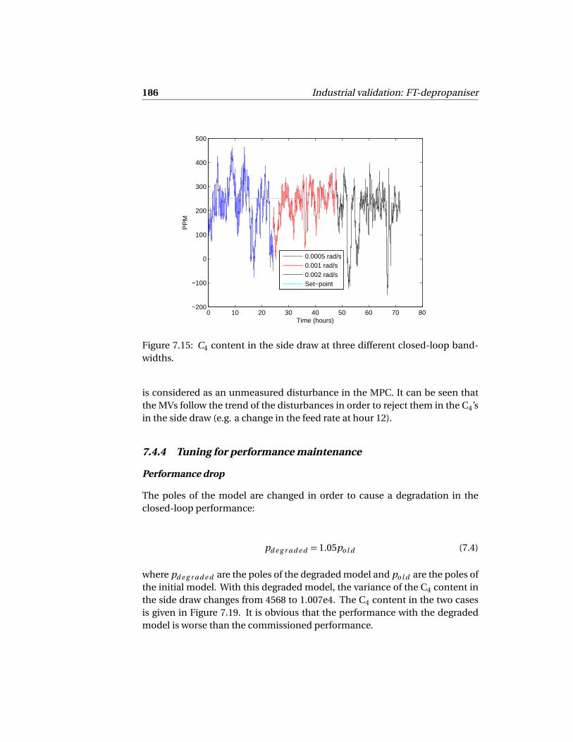
186 Industrial validation: FT-depropaniser
0 10 20 30 40 50 60 70 80−200
−100
0
100
200
300
400
500
Time (hours)
PP
M
0.0005 rad/s0.001 rad/s0.002 rad/sSet−point
Figure 7.15: C4 content in the side draw at three different closed-loop band-widths.
is considered as an unmeasured disturbance in the MPC. It can be seen thatthe MVs follow the trend of the disturbances in order to reject them in the C4’sin the side draw (e.g. a change in the feed rate at hour 12).
7.4.4 Tuning for performance maintenance
Performance drop
The poles of the model are changed in order to cause a degradation in theclosed-loop performance:
pd e g r a d e d = 1.05po l d (7.4)
where pd e g r a d e d are the poles of the degraded model and po l d are the poles ofthe initial model. With this degraded model, the variance of the C4 content inthe side draw changes from 4568 to 1.007e4. The C4 content in the two casesis given in Figure 7.19. It is obvious that the performance with the degradedmodel is worse than the commissioned performance.
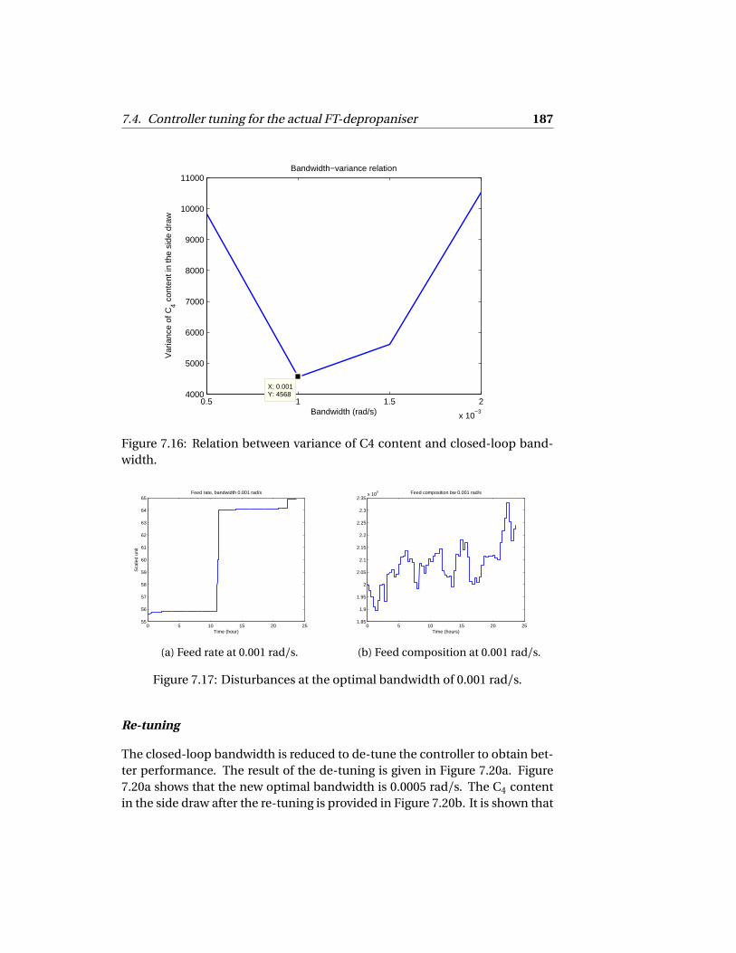
7.4. Controller tuning for the actual FT-depropaniser 187
0.5 1 1.5 2
x 10−3
4000
5000
6000
7000
8000
9000
10000
11000
X: 0.001Y: 4568
Bandwidth−variance relation
Bandwidth (rad/s)
Var
ianc
e of
C4 c
onte
nt in
the
side
dra
w
Figure 7.16: Relation between variance of C4 content and closed-loop band-width.
0 5 10 15 20 2555
56
57
58
59
60
61
62
63
64
65
Time (hour)
Feed rate, bandwidth 0.001 rad/s
Sca
led
unit
(a) Feed rate at 0.001 rad/s.
0 5 10 15 20 251.85
1.9
1.95
2
2.05
2.1
2.15
2.2
2.25
2.3
2.35x 10
5
Time (hours)
Feed composition bw 0.001 rad/s
(b) Feed composition at 0.001 rad/s.
Figure 7.17: Disturbances at the optimal bandwidth of 0.001 rad/s.
Re-tuning
The closed-loop bandwidth is reduced to de-tune the controller to obtain bet-ter performance. The result of the de-tuning is given in Figure 7.20a. Figure7.20a shows that the new optimal bandwidth is 0.0005 rad/s. The C4 contentin the side draw after the re-tuning is provided in Figure 7.20b. It is shown that

188 Industrial validation: FT-depropaniser
0 5 10 15 20 2558
60
62
64
66
68
70
72
74
76Side draw to feed ratio, bandwidth 0.001 rad/s
Time (hours)
%
(a) Side draw ratio at 0.001 rad/s.
0 5 10 15 20 2533
33.5
34
34.5
35
35.5
36Delta pressure, bandwidth 0.001 rad/s
kPa
Time (hours)
(b) Delta pressure at 0.001 rad/s.
Figure 7.18: MVs at the optimal bandwidth of 0.001 rad/s.
0 5 10 15 20 25−100
0
100
200
300
400
500
600
Time (hours)
PP
M
Bw 0.001 rad/s
Degraded modelSet−pointInitial model
Figure 7.19: C4 content in the side draw at the optimal bandwidth of 0.001rad/s.
re-tuning improves the closed-loop performance.

7.5. Conclusion 189
0 0.2 0.4 0.6 0.8 1
x 10−3
0.5
1
1.5
2
2.5
3
3.5
4x 10
4
Bandwidth (rad/s)
Var
ianc
e of
C4 c
onte
nt in
the
side
dra
w
(a) Relation between closed-loop band-width and output variance with degradedmodel.
0 5 10 15 20 250
100
200
300
400
500
600
Time (hours)
PP
M
At .0005 rad/sAt .001 rad/sSet−point
(b) C4 content in the side draw at 0.0005rad/s and 0.001 rad/s with degradedmodel.
Figure 7.20: Results of the re-tuning on the actual plant after a performancedrop arises.
7.5 Conclusion
An MPC was commissioned for the simulator and the actual FT-depropaniser.Step tests and RBS are used for the open-loop identification and based on pre-liminary knowledge about the open-loop system, the tuning method can findthe optimal closed-loop bandwidth at commissioning. On the simulator, theclosed-loop system is capable of rejecting low-frequency disturbances on theC4’s content in the side draw while respecting all the safety limits. On the ac-tual plant, the system has shown its ability of rejecting the disturbances in thefeed rate and feed composition. The convex relation between the closed-loopbandwidth and the variance of the key output is validated with the experimentsdone on both the simulator and the plant.
As for the re-tuning for performance maintenance, on the simulator, it isshown that when the model-plant mismatch is more significant, the new opti-mal bandwidth is lower than the initial one. It means the robustness takes pri-ority over the disturbance rejection and de-tuning the closed-loop system canretain the performance. However, further reducing the bandwidth increasesthe output variance again. Similar trends can be observed on the actual plantalthough the de-tuning experiment is limited to only more than 12 hours dueto technical issues in the communication between the process and the opera-tors’ control panel. The finding of the optimal closed-loop bandwidth at com-missioning and after a change in the plant dynamics also shows that an auto-tuning method using extremum seeking techniques as described in Chapter 3

190 Industrial validation: FT-depropaniser
is promising for industrial implementation, although it is not applied in theseexperiments due to the limited amount of time on the industrial site.
8Conclusions
8.1 Contributions 8.2 Future research directions
We conclude this thesis by summarising the main contributions and de-scribing a collection of possible directions and starting points for future re-search.
8.1 Contributions
A major challenge in the area of process control and optimisation is the main-tenance of advanced process controllers. Due to various problems, from in-strumentation incidents to changes in disturbances and process dynamics, ad-vanced process controllers fail to perform up to their capability. If proper main-tenance measures are not taken, the advanced process control system will beshut down more and more frequently by the operational staff. Of course, whichmaintenance measures to select depend on the source of the problems. Whileinstrumentation problems need specific tests on sensors and actuators, changesin the plant dynamics or disturbance characteristics require specific actionsin the advanced control level. These actions involve re-modelling and/or re-tuning stages. The analysis of the benefit of each corrective action is beyondthe scope of this thesis. The modelling and re-modelling are not investigatedeither. Instead, this thesis looks into the tuning and auto-tuning of advancedprocess controllers as part of a solution to the maintenance of model-basedoperations support systems. Nevertheless, tuning is by no means the unique

192 Conclusions
solution to the maintenance problem. Re-tuning the advanced process con-trollers may be of little use if the modelling errors are too significant. There-fore, tuning and auto-tuning should be considered as a complement to a largemaintenance scheme.
In the process industry, advanced process controllers are often overly de-tuned to guarantee smooth behaviour in the manipulated variables as well asrobustness at the commissioning phase. Despite the robustness this tuningcould provide, it usually operates the process far from the best trade-off be-tween nominal performance and robustness. Hence, the potential of the con-troller is not fully exploited. On the other hand, if the controller is tuned aroundthe optimum between performance and robustness, gradual changes in theplant dynamics can make this tuning become overly aggressive. This case iseven more critical than the case of overly sluggish control action, since theaggressiveness of the control action in the presence of high model-plant mis-match can lead to instability. Therefore, it is vital that the controller operates atthe optimum, but also keeps track of any changes in the disturbances or plantdynamics that can alter this optimum.
With this observation in mind, the first contribution of the thesis is the de-velopment of a practical auto-tuning method that aims to find the optimal bal-ance between the nominal performance of the closed-loop system and its ro-bustness. This balance is represented by the optimal closed-loop bandwidthof the system. The output variance is considered as the performance index forthe auto-tuning method. The input weight is perturbed with sine wave sig-nals to find the minimum of the mapping from the input weight to the out-put variance. The basis of this perturbation-based auto-tuning method is theextremum seeking, a model-free optimisation technique. By continuously ex-citing the input weighting factor without affecting the variance of the processoutputs significantly, the auto-tuning approach can adapt to changes in thesystem that cause the optimum to move. This auto-tuning method can reducethe effort of the control engineers and operators in tuning the control systems.It also gives an idea of how large the model-plant mismatch is, and thereforemakes a significant contribution to the whole maintenance scheme. For ex-ample, one could use that information together with other diagnosis methodsto investigate whether re-modelling the process is necessary and beneficial.
The existence of the optimal tuning has been validated on an industrial FT-depropaniser. It is a distillation column that separates C3’s and lighter com-ponents from C4’s and heavier components in the feed stream. On a simula-tor that duplicates the exact behaviour of the actual plant, the optimal trade-off between performance and robustness was found. When the model-plantmismatch becomes higher, de-tuning the controller could find the new op-

8.1. Contributions 193
timal closed-loop bandwidth. The optimal closed-loop bandwidth was alsofound on the actual plant during commissioning. However, due to the limitedtime available on the plant, the auto-tuning method has not been tested on theplant.
While the performance of the process and the tuning of advanced processcontrollers are usually described in the time domain, the natural behaviour ofthe process is often described in the frequency domain. For example, the op-timal tuning for the controller corresponds to the frequency-domain optimalclosed-loop bandwidth. Therefore, the theoretical contribution of the thesisfocuses on the frequency-domain aspects of the tuning. This thesis uses thismatching method to match an H∞ controller and the tuning of MPC becomesthe tuning of the weighting filters of the H∞ controller, which give more in-sights into the frequency-domain characteristics of the system. The matchingof MPC to a linear time-invariant controller in the state-space formulation wasinvestigated in literature (Hartley and Maciejowski (2011, 2013)). This match-ing, which is also called reverse-engineering tuning, allows the MPC to inheritthe properties of the linear time-invariant controller.
The thesis contributes to the area of reverse-engineering tuning by inves-tigating the matching of GPC with a linear time-invariant controller formu-lated in transfer functions. Due to the formulation in transfer functions, thismatching deals with the direct feed-through in the favourite controller in a di-rect way. This piece of research also shows that with some specific choices ofthe horizon, not every linear time-invariant behaviour can be achieved by theGPC when a quadratic cost function is used.
A novel perspective on the connection between the finite time domain andfrequency domain is provided in the thesis. The behaviour of the Toeplitz ma-trix that links the future inputs and future outputs is investigated. It is shownthat any changes in the input weights can be translated as changes in the sin-gular value matrix of the Toeplitz matrix. Along those lines, a number of workson tuning methods in literature have already dealt with the conditioning of thesystem matrix. Chapter 6 replicates and analyses an example in Goodwin et al.(2005), in which a tuning method based on changing the singular values ofthe Toeplitz matrix was proposed. It was shown that the frequency-domaincharacteristics of a controller do not directly relate to the singular values of theToeplitz matrix, despite the known connection between them and the open-loop gain of the system. Therefore, this thesis further analyses the SVD of theToeplitz matrix and shows that the phase properties of the system can be foundin its singular vectors. The link between the finite time domain and infinitetime domain is also further investigated.

194 Conclusions
8.2 Future research directions
The practical auto-tuning method presented in Chapter 3 of the thesis only per-turbs one tuning parameter and finds the best balance between input and out-put weights. When only one parameter is perturbed, the result of the extremumseeking method is a sub-optimal solution. If multiple weights on multiple in-puts are perturbed with dither signals at the same time, a global minimum ofthe output variance as a function of multiple input weights can be achieved.How to perturb multiple input weights at the same time to find the global min-imum will be considered in future research. Intuitively, the dither signals ap-plied to the different inputs should also be different and independent.
In addition, a challenge of all extremum seeking applications is the choiceof the amplitude and frequency of the dither signals to guarantee stability androbustness of the optimisation. This selection also affects the speed of con-vergence of the optimisation method. To increase the speed of convergence,an extremum seeking method based on Newton-like optimisation can be con-sidered. Such an approach will vary the size of the steps that the input weighttakes towards the optimum. For example, if the input weight is still far fromthe optimum, a large step is taken and vice versa.
Once these challenges are tackled, the auto-tuning method could be imple-mented on an actual industrial process. Such a test will require time and safetymeasures. The advantage of the auto-tuning method is that it does not dependon any specific MPC formulations or commercial products. Therefore, it canbe adapted to different MPC products in industry. However, the parameters ofthe method such as amplitude and frequency of the sinusoidal perturbationhave to be specifically computed for a specific MPC formulation.
Chapters 4 and 5 of the thesis deal with the reverse-engineering tuningmethods of MPC. However, these methods often consider the case of inactiveconstraints. Once an input of the system becomes saturated, the other inputsare used to control the process and the dynamics of the process can change.This case will be considered in future research.
The controller matching tuning method of GPC presented in Chapter 5 onlyconsiders plants with the same number of inputs and outputs. The approach tonon-square plants is similar, however, the feasibility condition of the matchingwill change. Different choices of the horizon will result in the matching prob-lem being feasible. Specific computation of these choices is an open researchdirection.
Regarding the investigation into the Toeplitz matrix shown in Chapter 6 ofthe thesis, the challenge is the synthesis of the controller (i.e. the tuning ofthe MPC) based on the available insights. The thesis has shown the link be-

8.2. Future research directions 195
tween the Toeplitz matrix and the open-loop characteristics. Intuitively, theMPC controller is the approximate inverse of the open-loop plant model. Theplant model is often inaccurate at high frequencies and therefore the inversionof the model is preferably taken at a limited frequency range. The connectionprovided in Chapter 6 can help to find a way to perform that "limited inversion"in the time domain. An advantage of the design in the time domain is that con-straints can then be handled explicitly since all the constraints on the signalsare described in the time domain. An example of this constraint handling isthe work of Rojas et al. (2004). However, as also shown in Chapter 6, the re-ceding horizon principle in the finite time domain makes the link between thefrequency-domain properties of the closed-loop system and the time-domainToeplitz matrix disappear. How to restore this link is still an open question.

196 Conclusions

Bibliography
Åkesson, J., January 2006. MPCtools 1.0 - Reference Manual. Department ofAutomatic Control, Lund Institute of Technology, Lund, Sweden.
Al-Ghazzawi, A., E., E. A., Nouh, A., Zafiriou, E., June 2001. On-line tuning strat-egy for model predictive controllers. Journal of Process Control 11 (3), 265–284.
Alazard, D., Apkarian, P., February 1999. Exact observer-based structures for ar-bitrary compensators. International Journal of Robust and Nonlinear Con-trol 9 (2), 101–118.
Albertos, P., Ortega, R., 1989. On generalized predictive control: Two alternativeformulations. Automatica 25 (5), 753–755.
Amrhein, M., Allgower, F., Marquardt, W., June-July 1993. Validation and anal-ysis of linear distillation models for controller design. In: Proceedings of the1993 European Control Conference. Groningen, The Netherlands, pp. 221–232.
An, A., Hao, X., Zhao, C., Su, H., August 2009. A pragmatic approach for se-lecting weight matrix coefficients in model predictive control algorithm andits application. In: Proceedings of the IEEE International Conference on Au-tomation and Logistics (ICAL 09). Shenyang, China, pp. 486–492.
Anderson, B., Moore, J., 1971. Linear Optimal Control. Prentice Hall.

198 Conclusions
Annergren, M., Kauven, D., Larsson, C. A., Potters, M., Tran, Q., Özkan, L., De-cember 2013. On the way to autonomous model predictive control: A dis-tillation column simulation study. In: Proceedings of the 10th InternationalSymposium on Dynamics and Control of Process Systems (DYCOPS). Mum-bai, India.
Backx, A., 2008. Modelling and predictive control: Introduction. Lecture Notes,Eindhoven University of Technology, the Netherlands.
Bagheri, P., Sedigh, A. K., September 2013. Analytical approach to tuning ofmodel predictive control for first-order plus dead time models. IET ControlTheory & Applications 7 (14), 1806–1817.
Banerjee, P., Shah, S., December 1992. Tuning guidelines for robust generalizedpredictive control. In: Proceedings of the 31st Conference on Decision andControl. Tucson, AZ, USA, pp. 3233–3234.
Bauer, M., Craig, I. K., January 2008. Economic assessment of advanced processcontrol - a survey and framework. Journal of Process Control 18 (1), 2–18.
Brown, R. G., Hwang, P. Y. C., December 1996. Introduction to Random Signalsand Applied Kalman Filtering, 3rd Edition. Vol. John Wiley & Sons. Wiley.
Cairano, S. D., Bemporad, A., January 2010. Model predictive control tuning bycontroller matching. IEEE Transactions on Automatic Control 55 (1), 185–190.
Chiou, H.-W., Zafiriou, E., June-July 1994. Frequency domain design of ro-bustly stable constrained model predictive controllers. In: Proceedings ofthe American Control Conference. Baltimore, MD, USA, pp. 2852–2856.
Chmielewski, D. J., Manthanwar, A. M., October 2004. On the tuning of predic-tive controllers: Inverse optimality and the minimum variance covarianceconstrained control problem. Ind. Eng. Chem. Res. 43 (24), 7807–7814.
Chow, C. M., Kuznetsov, A. G., Clarke, D. W., 1995. Application of generalisedpredictive control to the paper machine benchmark. Control EngineeringPractice 3 (10), 1483–1486.
Clarke, D. W., April 1988. Application of generalized predictive control to indus-trial processes. IEEE Control Systems Magazine 8 (2), 49–55.
Clarke, D. W., Mohtadi, C., 1989. Properties of generalized predictive control.Automatica 25 (6), 859–875.

8.2. Future research directions 199
Clarke, D. W., Mohtadi, C., Tuffs, P. S., March 1987a. Generalized predictive con-trol - part i. the basic algorithm. Automatica 23 (2), 137–148.
Clarke, D. W., Mohtadi, C., Tuffs, P. S., March 1987b. Generalized predictive con-trol - part ii. extensions and interpretations. Automatica 23 (2), 149–160.
Cutler, C. R., 1983. Dynamic matrix control: An optimal multivariable controlalgorithm with constraints. Phd thesis, Univ. of Houston.
Cutler, C. R., Ramaker, B. L., August 1980. Dynamic matrix control - a computercontrol algorithm. In: Proceedings of the Joint Automatic Control Confer-ence. San Francisco, CA, USA.
Dougherty, D., Cooper, D. J., 2003. Tuning guidelines of a dynamicmatrix controller for integrating (non-self-regulating) processes.Ind.Eng.Chem.Res (42), 1739–1752.
Doyle, J. C., Stein, G., August 1978. Robustness with observers. IEEE Transac-tions on Automatic Control 24 (4), 607 – 611.
Drogies, S., Geest, D. D., June 1999. Predictive control: Propositions for the de-sign methodology. In: Procceedings of the American Control Conference.San Diego, CA, USA, pp. 647–651.
Edouard, D., Dufour, P., Hammouri, H., 2005. Observer based multivariablecontrol of a catalytic reserve flow reactor: Comparison between lqr and mpcapproaches. Comput. Chem. Eng. 29, 851–865.
Exadaktylos, V., Taylor, C. J., 2010. Multi-objective performance optimisationfor model predictive control by goal attainment. International Journal ofControl 83 (7), 1374–1386.
Fan, J., Stewart, G., Aug. 18 2009. Automatic tuning method for multivariablemodel predictive controllers. US Patent 7,577,483.URL http://www.google.com/patents/US7577483
Ford, N. J., Savostyanov, D. V., Zamarashkin, N. L., October 2014. On the de-cay of elements of inverse triangular Toeplitz matrix. SIAM Journal on MatrixAnalysis and Applications 35 (4), 1288–1302.
Freudenberg, J. S., Looze, D. P., 1988. Frequency Domain Properties of Scalarand Multivariable Feedback Systems. Springer-Verlag.
Friedman, Y. Z., January 2005. Has the advanced process control industry com-pletely collapsed? Hydrocarbon Processing, 15–16.

200 Conclusions
Gahinet, P., Apkarian, P., December 1993. An lmi-based parametrization of allh∞ controllers with applications. In: Proceedings of the 32nd Conferenceon Decision and Control. San Antonio, TX, USA, pp. 656–661.
Garriga, J. L., Soroush, M., June 2008. Model predictive controller tuning viaeigenvalue placement. In: Proceedings of the 2008 American Control Con-ference. Seattle, WA, USA, pp. 429–434.
Garriga, J. L., Soroush, M., March 2010. Model predictive control tuning meth-ods: A review. Ind. Eng. Chem. Res. 49 (8), 3505–3515.
Gary, J. H., Handwerk, G. E., 2001. Petroleum Refining: Technology and Eco-nomics, 4th Edition. CRC Press.
Goodwin, G. C., Seron, M. M., Doná, J. A. D., 2005. Constrained Control andEstimation: An Optimisation Approach. Springer.
Guidi, H., Larsson, C., Tran, Q., December 2013. Results on the sasol validationcase. Deliverable D6.4, Autoprofit project.
Han, K., Zhao, J., Qian, J., June 2006. A novel robust tuning strategy for modelpredictive control. In: Proceedings of the 6th World Congress on IntelligentControl and Automation. Dalian, China, pp. 6406–6410.
Hartley, E. N., Maciejowski, J. M., August 2009. Initial tuning of predictive con-trollers by reverse engineering. In: Proceedings of the European ControlConference. Budapest, Hungary.
Hartley, E. N., Maciejowski, J. M., September 2011. Designing mpc controllersby reverse-engineering existing lti controllers. Technical report, CambridgeUniversity Engineering Department, Cambridge, UK.
Hartley, E. N., Maciejowski, J. M., November 2013. Designing mpc controllersby reverse-engineering existing lti controllers. IEEE Transactions on Auto-matic Control 58 (11), 2934–2939.
Hasegawa, A., August 1994. Development of a strip temperature control systemwith adaptive generalized predictive control. In: Proceedings of the thirdIEEE Conference on Control Applications. Glasgow, UK, pp. 1525–1531.
Hinde, R. F., Cooper, D. J., 1994. A pattern-based approach to excitation diag-nostics for adaptive process control. Chem. Eng. Sci. 49 (9), 1403–1415.

8.2. Future research directions 201
Huusom, J. K., Poulsen, N. K., Jørgensen, S. B., Jørgensen, J. B., 2010. Arx-modelbased model predictive control with offset-free tracking. Computer AidedChemical Engineering 28, 601–606.
Huusom, J. K., Poulsen, N. K., Jørgensen, S. B., Jørgensen, J. B., December 2012.Tuning siso offset-free model predictive control based on arx models. Jour-nal of Process Control 22 (10), 1997–2007.
Iino, Y., Tomida, K., Fujiwara, H., Takagi, Y., Shigemasa, T., Yamamoto, A.,November 1993. A new input/output constrained model predictive controlwith frequency domain tuning technique and its application to an ethyleneplant. In: Proceedings of the International Conference on Industrial Elec-tronics, Control, and Instrumentation (IECON) 1993. Maui, HI, USA, pp.457–462.
Johansson, K. H., 1997. Relay feedback and multivariable control. Phd thesis,Lund Institute of Technology, Sweden.
Kalman, R. E., March 1964. When is a linear control system optimal? Journal ofBasic Engineering 86 (1), 51–60.
Karacan, S., Hapoglu, H., Alpbaz, M., 2001. Application of optimal adaptivegeneralized predictive control to a packed distillation column. Chemical En-gineering Journal 84, 389–396.
Killingsworth, N. J., Krstic, M., February 2006. Pid tuning using extremum seek-ing: online, model-free performance optimization. IEEE Control SystemsMagazine 26 (1), 70–79.
Kotze, G., Chetty, C., Simbanegavi, S., July 2011. Advanced Control and Op-timisation (ACO) for SCC FT depropanizer. Advanced process control: As-built document. SASOL Synthetic Fuels (Pty) Ltd, Honeywell Automationand Control Solutions South Africa (Pty) Ltd, PO Box 6674, Midrand 1685,South Africa.
Kreindler, E., Jameson, A., June 1972. Optimality of linear control systems. IEEETransactions on Automatic Control 17 (3), 349 – 351.
Krstic, M., Wang, H., April 2000. Stability of extremum seeking feedback forgeneral nonlinear dynamic systems. Automatica 36 (1), 595–601.
Larsson, C., Annergren, M., Hjalmarsson, H., Rojas, C., Bombois, X., Mesbah,A., Modén, P. E., July 2013. Model predictive control with integrated experi-

202 Conclusions
ment design for output error systems. In: Proceedings of the 2013 EuropeanControl Conference. Zurich, Switzerland, pp. 3790–3795.
Lee, J. H., Yu, Z. H., 1994. Tuning of model predictive controllers for robust per-formance. Comput. Chem. Eng. 18 (1), 15–37.
Lee, J. H. V. D., Svrcek, W. Y., Young, B. R., 2008. A tuning algorithm for modelpredictive controllers based on genetic algorithms and fuzzy decision mak-ing. ISA Transactions 47, 53–59.
Levya, R., Artillan, P., Cabal, C., Estibals, B., Alonso, C., April 2011. Dynamicperformance of maximum power point tracking circuits using sinusoidal ex-tremum seeking control for photovoltaic generation. International Journalof Electronics 98 (4), 529–542.
Liu, W., Wang, G., October 2000. Auto-tuning procedure for model-based pre-dictive controller. In: Proceedings of the IEEE International Conference onSystems, Man, and Cybernetics. Nashville, TN, USA.
Löfberg, J., 2004. Yalmip : A toolbox for modeling and optimization in MATLAB.In: Proceedings of the Computer Aided Control System Design (CACSD)Conference. Taipei, Taiwan.URL http://users.isy.liu.se/johanl/yalmip
Ludlage, J. H., November 1997. Controllability analysis of industrial processes:towards the industrial application. Phd thesis, Eindhoven University of Tech-nology, the Netherlands.
Ludlage, J. H., Weiland, S., Stoorvogel, A. A., Backx, A. C. P. M., July 2003. Finite-time behavior of inner systems. IEEE Transactions on Automatic Control48 (7), 1134–1149.
Lundström, P., Skogestad, S., Wang, Z.-Q., January 1991a. Performance weightselection for h-infinity and mu-control methods. Transactions of the Insti-tute of Measurement and Control 13 (5), 241–252.
Lundström, P., Skogestad, S., Wang, Z.-Q., March 1991b. Weight selection forh∞ and mu-control methods - insights and examples from process control.In: Symposium on Robust Control System Deisgn Using H∞ and RelatedMethods. Cambridge, UK.
Maciejowski, J. M., 1989. Multivariable Feedback Design. Addison-Wesley Pub-lishers Ltd.

8.2. Future research directions 203
Maciejowski, J. M., 2002. Predictive control with constraints. Pierson, PrenticeHall.
Maurath, P. R., Mellichamp, D. A., Seborg, D. E., June 1988a. Predic-tive controller design for single-input/single-output (siso) systems.Ind.Eng.Chem.Res. 27 (6), 956–963.
Maurath, P. R., Seborg, D. E., Mellichamp, D. A., July 1988b. Predictive controllerdesign by principal components analysis. Ind. Eng. Chem. Res. 27 (7), 1204–1212.
McFarlane, D., Glover, K., June 1992. A loop-shaping design procedure usingh∞ synthesis. IEEE Transactions on Automatic Control 37 (6), 759–769.
McIntosh, A. R., Shah, S. L., Fisher, D. G., June 1989. Selection of tuning param-eters for adaptive generalized predictive control. In: Proceedings of the 1989American Control Conference. Pittsburgh, PA, USA, pp. 1846–1851.
McIntosh, A. R., Shah, S. L., Fisher, D. G., 1991. Analysis and tuning of adaptivegeneralized predictive control. Can. J. Chem. Eng. 69, 97–110.
Mesbah, A., Bombois, X., Ludlage, J., den Hof, P. V., July 2012. Experiment de-sign for closed-loop performance diagnosis. In: Proceedings of the 16th IFACSymposium on System Identification. Brussels, Belgium, pp. 1341–1346.
Moase, W. H., Manzie, C., Brear, M. J., September 2010. Newton-like extremum-seeking for the control of thermoacoustic instability. IEEE Transactions onAutomatic Control 55 (9), 2094–2105.
Nagrath, D., Prasad, V., Bequette, B. W., Isermann, H. P., June 2000. Model pre-dictive control of open-loop unstable cascade systems. In: Proceedings ofthe American Control Conference (ACC). Chicago, IL, USA.
Olesen, D. H., Huusom, J. K., Jørgensen, J. B., November 2012. Optimizationbased tuning approach for offset free mpc. In: Proceedings of the 10th Euro-pean Workshop on Advanced Control and Diagnosis (ACD 2012). Kgs. Lyn-gby, Denmark.
Olesen, D. H., Huusom, J. K., Jørgensen, J. B., June 2013. A tuning procedure forarx-based mpc of multivariate processes. In: Proceedings of the 2013 Amer-ican Control Conference. Washington, DC, USA.
Özkan, L., Meijs, J., Backx, A., 2012. A frequency domain approach for mpc tun-ing. In: Proceedings of the 11th International Symposium on Process Sys-tems Engineering. pp. 1632–1636.

204 Conclusions
Pieterse, F., Kotze, G., Simbanegavi, S., July 2011. Advanced Control and Opti-misation (ACO) for C3 distribution. FT depropanizer APC: Operator train-ing manual. SASOL Synthetic Fuels (Pty) Ltd, Honeywell Automation andControl Solutions South Africa (Pty) Ltd, PO Box 6674, Midrand 1685, SouthAfrica.
Prempain, E., Postlethwaite, I., 28 2001. Feedforward control: a full-information approach. Automatica 37 (1), 17.
Qin, S. J., Badgwell, T. A., January 2003. A survey of industrial model predictivecontrol technology. Control Engineering Practice 11, 733–764.
Rani, K. Y., Unbehauen, H., 1997. Study of predictive controller tuning meth-ods. Automatica 33 (12), 2243–2248.
Reverter, C. M., Ibarrola, J., Cano-Izquierdo, J.-M., 2014. Tuning rules for aquick start up in dynamic matrix control. ISA Transactions 53, 612–627.
Richalet, J., Rault, A., Testud, J. L., Papon, J., September 1978. Model predictiveheuristic control: Applications to industrial processes. Automatica 14 (5),413–428.
Rojas, O. J., Goodwin, G. C., June-July 2004. On the asymptotic properties ofthe hessian in discrete-time linear quadratic control. In: Proceedings of the2004 American Control Conference. Boston, MA, USA.
Rojas, O. J., Goodwin, G. C., Feuer, A., Serón, M. M., June 2003. A sub-optimalreceding horizon control strategy for constrained linear systems. In: Pro-ceedings of the 2003 American Control Conference. Denver, CO, USA.
Rojas, O. J., Goodwin, G. C., Serón, M. M., Feuer, A., September 2004. Ansvd based strategy for receding horizon control of input constrained linearsystems. International Journal of Robust and Nonlinear Control 14 (13-14),1207–1226.
Rossiter, J. A., 2005. Model-based Predictive Control: A practical approach.Control series. CRC Press.
Rowe, C., Maciejowski, J., June 2000a. Tuning mpc using h∞ loop shaping. In:Proceedings of the American Control Conference. Chicago, IL.
Rowe, C., Maciejowski, J. M., December 2000b. Robust finite horizon mpc with-out terminal constraints. In: Proceedings of the 39st IEEE Conference on De-cision and Control. Sydney, Australia, pp. 166–171.

8.2. Future research directions 205
Sasol, 2014. Official website of Sasol Limited.URL http://www.sasol.co.za/
Shah, G., Engell, S., June 2010. Tuning mpc for desired closed-loop perfor-mance for siso systems. In: Proceedings of the 18th Mediterranean Confer-ence on Control & Automation (MED). Marrakech, Morocco, pp. 628–633.
Shah, G., Engell, S., June-July 2011. Tuning mpc for desired closed-loop per-formance for mimo systems. In: Proceedings of the 2011 American ControlConference. San Francisco, CA, USA.
Shah, G., Engell, S., July 2013. Multivariable mpc design based on a frequencyresponse approximation approach. In: Proceedings of the 2013 EuropeanControl Conference. Zürich, Switzerland.
Shridhar, R., Cooper, D. J., 1997. A tuning strategy for unconstrained siso modelpredictive control. Ind. Eng. Chem. Res. 36, 729–746.
Shridhar, R., Cooper, D. J., 1998. A tuning strategy for unconstrained multivari-able model predictive control. Ind. Eng. Chem. Res. (37), 4003–4016.
Skogestad, S., 1997. Dynamics and control of distillation columns - a tutorialintroduction.
Skogestad, S., Morari, M., 1987. Effect of disturbance directions on closed-loopperformance. Ind.Eng.Chem.Res. 26, 2029–2035.
Skogestad, S., Morari, M., 1988. Robust control of ill-conditioned plants: High-purity distillation. IEEE Transactions on Automatic Control 33 (12), 1092–1105.
Skogestad, S., Postlethwaite, I., August 2005. Multivariable Feedback Control,2nd Edition. Wiley.
Stankovic, M. S., Stipanovic, D. M., August 2010. Extremum seeking understochastic noise and applications to mobile sensors. Automatica 46 (8),1242–1251.
Suzuki, R., Kawai, F., Ito, H., Nakazawa, C., Fukuyama, Y., Aiyoshi, E., April2007. Automatic tuning of model predictive control using particle swarm op-timization. In: Proceedings of the 2007 IEEE Swarm Intelligence Symposium.Honolulu, HI, USA.

206 Conclusions
Tan, Y., Moase, W. H., Manzie, C., Nesic, D., Mareels, I., July 2010. Extremumseeking from 1922 to 2010. In: Proceedings of the 29th Chinese Control Con-ference. Beijing, China, pp. 14–26.
Tan, Y., Nesic, D., Mareels, I., June 2006. On non-local stability properties ofextremum seeking control. Automatica 44 (5), 889–903.
Tan, Y., Nesic, D., Mareels, I., May 2008. On the choice of dither in extremumseeking systems: A case study. Automatica 44 (5), 1446–1450.
Tran, Q. N., Özkan, L., Backx, A., Autumn 2012. Mpc tuning based on impact ofmodelling uncertainty on closed-loop performance. In: Proceedings of the2012 AICHE Annual Meeting. Pittsburg, PA, USA.
Trierweiler, J. O., Farina, L. A., 2003. Rpn tuning strategy for model predictivecontrol. Journal of Process Control (13), 591–598.
Waschl, H., Alberer, D., del Re, L., February 2011a. Automatic tuning methodsfor mpc environments. In: Lecture Notes in Computer Science, Vol. 6928:EUROCAST 2011, 13th International Conference on Computer Aided Sys-tems Theory. Las Palmas de Gran Canaria, Spain, pp. 41–48.
Waschl, H., Alberer, D., del Re, L., August-September 2011b. Numerically effi-cient self tuning strategies for mpc of integral gas engines. In: Proceedingsof the 18th IFAC World Congress. Milano, Italy.
Wojsznis, W., Gudaz, J., Blevins, T., Mehta, A., 2003. Practical approach to tun-ing mpc. ISA Transactions 42, 149–162.
Yamamoto, T., Aoyama, J., Nakano, K., June 2003. A design of 2dof robust self-tuning gpc. In: Proceedings of the 2003 IEEE International Symposium onIndustrial Electronics (ISIE). Rio de Janeiro, Brazil, pp. 566–571.
Yoshitani, N., Hasegawa, A., March 1998. Model-based control of strip temper-ature for the heating furnace in continuous annealing. IEEE Transactions OnControl Systems Technology 6 (2), 1998.
Zhou, K., Doyle, J. C., Glover, K., 1996. Robust and Optimal Control. PrenticeHall, New Jersey 07458.
Zhu, Y., Backx, A., 1993. Identification of multivariable industrial processes forsimulation, diagnosis, and control. Springer-Verlag.

Appendices


AAppendix to Chapter 2
A.1 Relation between MPC tuning and model uncertainty
This section presents an analysis of the relation between the tuning of MPCand model uncertainty. The MPC cost function is represented as functions ofsensitivity, complementary sensitivity functions and weighting matrices. Thesame impact of uncertainty in robust controllers was observed in MPC. In ro-bust control theory, the sensitivity and complementary sensitivity functionsare tuned to adjust the closed-loop bandwidth. In the case of MPC, the closed-loop bandwidth is determined by the weighting matrices on the CV’s and MV’s.The analysis is illustrated with a quadruple tank example introduced in Johans-son (1997) and Åkesson (2006). A diagram of an MPC as an output feedbackcontroller (Figure A.1) helps to analyse frequency-domain characteristics of thesystem. The transfer functions on the diagram are given by:
H (z ) =−Ks x Hy (z ) (A.1)
K (z ) =
I −1
z −1Ks u −
z
z −1Ks x Hu (z )
−1
(A.2)
and
P (z ) =C (z I −A)−1B (A.3)
Hy (z ) = (z I −A+Ko b s C )−1Ko b s (A.4)
Hu (z ) = (z I −A+Ko b s C )−1B (A.5)

210 Appendix to Chapter 2
K(z) P(z)Δu(k) y(k)
H(z)
e(k)
-1
Figure A.1: Block diagram of MPC
where Ks u , Ks x and Ko b s are found in (2.40) and (2.42).The frequency-domain characteristics of MPC described here are based on
Tran et al. (2012) and Özkan et al. (2012). Consider an input disturbance e (k )of white-noise type, which is unmeasurable and generates the variance on theoutput:
x (k +1) = Ax (k ) +B u (k ) +Be e (k ) (A.6)
In the following, to investigate the effect of the weighting factors on the closed-loop bandwidth of the MPC, assume that the weighting matrices in cost func-tion (2.32) are Q = I , R =ρI and the prediction horizon is equal to the controlhorizon Hp =Hu =N . The cost function can then be written as:
J (k ) = ‖Y (k )‖22+ρ ‖∆U ‖2
2 (A.7)
where ‖X ‖2 denotes the Euclidean norm of vector X = [x1, x2, . . . , xn ]:
‖X ‖2 =
√
√
√
n∑
i=1
x 2i . (A.8)
Based on Parseval’s theorem, it follows that:
J (k ) =1
N
N−1∑
k=0
|Y [k ]|2+ρ
N
N−1∑
k=0
|∆U [k ]|2 (A.9)

A.1. Relation between MPC tuning and model uncertainty 211
where Y [k ] and ∆U [k ] are the DFT of y (k + i |k ) and ∆u (k + i |k ). Note thatΦY (ωk ) =
1N |Y [k ]|
2 andΦ∆U (ωk ) =1N |∆U [k ]|2 are the power spectral functions
of the output signal and input increments at frequencyωk =kN ωs whereωs is
the sampling frequency. Therefore:
J (k ) =N−1∑
k=0
ΦY (ωk ) +ρN−1∑
k=0
Φ∆U (ωk ). (A.10)
Due to the assumption that the power of the output and input signals are gen-erated by the white-noise signals e (k ),
ΦY (ωk ) = ‖Ty e (ejωk )‖2
2
Φ∆U (ωk ) = ‖T∆ue (ejωk )‖2
2 (A.11)
where Ty e (e jωk ) and T∆ue (e jωk ) are the transfer function from e (k ) to y (k ) and∆u (k ) at frequencyωk , respectively. Hence the cost function J (k ) can be writ-ten as follows:
J (k ) = ‖Ty e ‖22+ρ‖T∆ue ‖2
2 (A.12)
where ‖Ty e ‖2 and ‖T∆ue ‖2 are the H2 norm of Ty e and T∆ue over the frequencyrange ωk for k = 0; 1; . . . ; N − 1. These transfer functions are computed as fol-lows. The transfer function from e (k ) to x (k ) is given by
Tx e = (z I −A+B K H C )−1 Be . (A.13)
The transfer function from e (k ) to the output y (k ) is given by
Ty e =C (z I −A+B K H C )−1 Be (A.14)
=C
I + (z I −A)−1B K H C−1(z I −A)−1Be (A.15)
=
I +C (z I −A)−1B K H−1
C (z I −A)−1Be (A.16)
= (I +P K H )−1 Pe . (A.17)
where P is the transfer function from u (k ) to y (k ) and Pe = C (z I − A)−1Be .Since∆u (k ) = K H y (k ), the transfer function from e (k ) to the output∆u (k ) isgiven by

212 Appendix to Chapter 2
T∆ue = K H (I +P K H )−1 Pe . (A.18)
Define the sensitivity function S = (I +P K H )−1 and complementary sensi-tivity function T = P K H (I +P K H )−1. As P and Pe do not depend on the con-troller, the dependency of frequency-domain characteristics of Ty e and T∆ue
on the weighting factor ρ is the same as the dependency of the frequency-domain characteristics of S and T . Since S+T = I , it is impossible to make both‖Ty e ‖2
2 and ‖T∆ue ‖22 small. That is to say that the factor ρ decides the trade-off
between the input energy and output energy of the closed-loop system. LetΩr
be the range of frequency in which σ(S ) < 1, where σ(S ) is the maximum sin-gular value of the sensitivity function S . When ρ is reduced, Ωr expands and alarge-bandwidth controller is obtained and vice versa. To summarise, tuningρ directly affects the closed-loop bandwidth of the system. Hence, without thepresence of model uncertainty, reducingρ (namely increasing the closed-loopbandwidth) leads to a low output variance. A high value ofρ (i.e. a low closed-loop bandwidth) results in low input energy and the effect of disturbances onthe outputs will become significant.
Consider now two types of uncertainty that cause the model-plant mis-match: The multiplicative input and output uncertainty. The real plant is thengiven by
• P ′ = (I +W∆)P in the case of output uncertainty
• P ′ = P (I +W∆) in the case of input uncertainty
where∆ represents the normalised uncertainty bound whose norm is no greaterthan 1 and W is the uncertainty weight which represents the frequency prop-erty of the uncertainty. The transfer functions Ty e and T∆ue are given by:
Output uncertainty
Ty e =
I +P ′K H−1(I +We∆e )Pe (A.19)
= [I + (I +W∆)P K H ]−1 (I +We∆e )Pe (A.20)
=
I +W∆P K H (I +P K H )−1
(I +P K H )−1(I +We∆e )Pe (A.21)
= S (I +W∆T )−1(I +We∆e )Pe . (A.22)
Input uncertainty (for a square plant)
Ty e = (I +P (I +W∆)K H )−1 (I +We∆e )Pe (A.23)

A.2. Example: Quadruple tank 213
=
I +
I +P W∆P −1
P K H−1(I +We∆e )Pe (A.24)
=
I +P W∆P −1P K H (I +P K H )−1
(I +P K H )−1(I +We∆e )Pe (A.25)
= S
I +P W∆P −1T−1(I +We∆e )Pe . (A.26)
Assume that the amplitude of the uncertainty weight W is significant atfrequencyωu , in this case, decreasing ρ (increasing the bandwidth) increasesthe range Ωr where σ(S )< 1. In addition:
σ(S ) + σ(T )≥ σ(S +T ) = 1 (A.27)
Hence, the biggerΩr , the bigger the region where σ(T )≈ 1 becomes. Whenthis region covers ωu due to a small ρ, the difference between the sensitivityfunction of the model and that of the plant becomes considerable, due to (A.22)and (A.26). Therefore, increasing the bandwidth improves the low-frequencydisturbance rejection, but gives low stability margin as well as ringing behaviourand makes the closed-loop system become sensitive to modelling errors andhigh-frequency measurement noise. As a result, the output energy ‖Ty e ‖2
2 canincrease again and there exists a balance between disturbance rejection androbustness.
A.2 Example: Quadruple tank
A.2.1 Introduction to the quadruple tank
A quadruple-tank laboratory process, originally presented in Johansson (1997),is used to illustrate the impact of modelling errors on the closed-loop perfor-mance of MPC. This investigation is developed from the linearisation of thequadruple-tank process and the implementation of MPC described in Åkesson(2006). A schematic view of the quadruple tank is given in Figure A.2. The pro-cess consists of four tanks, two upper tanks and two lower ones. A water con-tainer below the tanks is connected to two pumps which are used to pour waterinto the tanks. Pump 1 pours water into tank 1 and 4, while pump 2 pours wa-ter into tank 2 and 3. Two valves are used to manipulate the amount of waterpoured into the upper and lower tanks.
The states of the dynamic system x1, x2, x3 and x4 are the water levels inthe corresponding tanks (in cm). The upper limits of these levels are 20 cm.The MV’s are the pump voltages and the CV’s are the water levels in tank 1 andtank 2. Details of the discretisation and linearisation can be found in Åkesson(2006). The 2×2 discrete linearised model is given by:

214 Appendix to Chapter 2
Figure A.2: Schematic view of the quadruple tank.

A.2. Example: Quadruple tank 215
Table A.1: Parameters of the quadruple tank model
Parameters Values Unit
A1; A2 28 [cm2]A3; A4 32 [cm2]a1; a2 0.071 [cm2]a3; a4 0.057 [cm2]k1; k2 3.33;3.35 [cm3/Vs]
kc 0.50 [V/cm]g 981 [cm/s2]
γ1;γ2 0.25; 0.35
Table A.2: Operating conditions of the quadruple tank
Variables Values Unit
x 01 ; x 0
2 8.2444;19.0163 [cm]x 0
3 ; x 04 4.3146;8.8065 [cm]
u 01 ; u 0
2 3;3 [V]
∆x =
− 1T1
0 A4A1T3
0
0 − 1T2
0 A4A2T4
0 0 − 1T3
00 0 0 − 1
T4
∆x +
γ1k1A1
0
0 γ2k2A2
0 (1−γ2)k2A3
(1−γ1)k1A4
0
∆u
∆y =
kc 0 0 00 kc 0 0
∆x
(A.28)
where Ti =Aiai
r
2x 0i
g ;∆x = x − x 0;∆u = u −u 0 and∆y = y − y 0. The samplingtime of the model is 3 seconds. The parameters of the quadruple tank modelare given in Table A.1 and the operating conditions x 0 and u 0 are given in TableA.2.
An MPC is implemented to fulfil the control objectives while satisfying theconstraints. The basic parameters of the MPC are provided in Table A.3 andmore details of the commissioning of the MPC can be found in Åkesson (2006).Notice that the size of the state noise covariance matrix is 6×6 due to the stateextension for integral action. In this example, ρ is used to change the closed-loop bandwidth of the system and show the relation between the closed-loop

216 Appendix to Chapter 2
Table A.3: Parameters of the MPC on the quadruple tank
Parameter Meaning Value
Hp Prediction horizon 30Hu Control horizon 10Q Weighting matrix on output errors diag(2,1)R Weighting matrix on input increments ρ diag(1,1)W Process noise covariance matrix diag(1,1,1,1,1,1)V Measurement noise covariance matrix diag(0.01,0.01)
10−5
10−4
10−3
10−2
10−1
100
101
−100
−80
−60
−40
−20
0
20
Singular Values
Frequency (rad/s)
Sin
gula
r V
alue
s (d
B)
rho = e−2
rho = 1
rho = 100
rho = e+4
(a) Sensitivity function S .
10−5
10−4
10−3
10−2
10−1
100
101
−90
−80
−70
−60
−50
−40
−30
−20
−10
0
10
Singular Values
Frequency (rad/s)
Sin
gula
r V
alue
s (d
B)
rho = e−2
rho = 1
rho = 100
rho = e+4
(b) Complementary sensitivity functionT = I −S .
Figure A.3: Sensitivity function and complementary sensitivity function of thequadruple tank system with different values of ρ.
bandwidth and the modelling errors. Since the disturbance model is not in-cluded in the model, the sensitivity function S and complementary sensitivityfunction T are studied instead of the transfer functions Ty e and Tue . Relations(A.17) and (A.18) show that the changes in the bandwidths of S and T also re-flect the same changes in the bandwidths of Ty e and Tue .
The sensitivity function S and complementary sensitivity functions T =I −S of the MPC with different values of ρ are given in Figure A.3. It is shownthat the relation between ρ and the closed-loop bandwidth is a bijection: In-creasing ρ lowers the closed-loop bandwidth and reducing ρ raises it.
A.2.2 Effect of model uncertainty on closed-loop performance
Assume that the actual system belongs to the following model sets:

A.2. Example: Quadruple tank 217
Table A.4: Characteristics of the uncertainty weight w (z )
Low-frequency gain Bandwidth [rad/s] High-frequency gain
0.01 0.05 10
10−4
10−3
10−2
10−1
100
101
−4
−3
−2
−1
0
1
2
3
4
5
Singular Values
Frequency (rad/s)
Sin
gula
r V
alue
s (d
B)
(a) 1+δ1w (z ).
10−4
10−3
10−2
10−1
100
101
−4
−3
−2
−1
0
1
2
3
Singular Values
Frequency (rad/s)
Sin
gula
r V
alue
s (d
B)
(b) 1+δ2w (z ).
Figure A.4: Uncertainty sets 1+δ1w (z ) and 1+δ2w (z ).
P = (I +W (z )∆)P (A.29)
where ∆ =
δ1 00 δ2
represents arbitrary LTI dynamics with frequency re-
sponse gain no larger than one; W (z ) =
w (z ) 00 w (z )
and w (z ) is a transfer
function defining the frequency distribution of the uncertainty. The character-istics of w (z ) are given in Table A.4. The characteristics of w (z ) indicate thatthe model is uncertain at high frequencies, which is characteristic of processmodelling since the low-frequency behaviour of the process is more likely tobe captured by identification. This is also reflected by the singular value plotsof 1+δ1w (z ) and 1+δ2w (z ) in Figure A.4.
To study the effect of the uncertainty set on the sensitivity and complemen-tary sensitivity functions, ρ = 100 and ρ = 0.01 are by turns chosen. The otherparameters are given in Table A.3. The sensitivity function S and complemen-tary sensitivity function T for two different values of ρ are given in Figure A.5aand A.5b, respectively. It is shown that the effect of the uncertainty is significantat high frequencies on both functions. Furthermore, at the higher bandwidth(corresponding toρ = 0.01), the impact of modelling errors is much more con-

218 Appendix to Chapter 2
10−4
10−3
10−2
10−1
100
101
−80
−60
−40
−20
0
20
40
Singular Values
Frequency (rad/s)
Sin
gula
r V
alue
s (d
B)
rho = 100
rho = 0.01
(a) Sensitivity function S .
10−4
10−3
10−2
10−1
100
101
−60
−50
−40
−30
−20
−10
0
10
20
30
Singular Values
Frequency (rad/s)
Sin
gula
r V
alue
s (d
B)
rho = 100
rho = 0.01
(b) Complementary sensitivity function T .
Figure A.5: Singular values of the sensitivity function and complementary sen-sitivity function for ρ = 100 and ρ = 0.01.
siderable. This indicates that by increasing the closed-loop bandwidth, the sys-tem will be more and more sensitive to model-plant mismatch and the outputvariance will rise.
From the set of uncertain sensitivity functions, the function with the high-est peak over the whole frequency range is assumed to be the actual process.The MPC using the initial model for prediction is applied to both the initialmodel and the actual process at different closed-loop bandwidths to show therelation between the model-plant mismatch and closed-loop bandwidth. Alow-pass-filtered white noise with an amplitude of 5 V and a crossover fre-quency of 0.52 rad/s is added to the MV’s of the system. Figure A.6 shows therelation between the closed-loop bandwidth and the output variance in twocases: With model-plant mismatch and without model-plant mismatch. Theresults show that if the model and process are exactly the same, increasing theclosed-loop bandwidth reduces the output variance. However, in the presenceof modelling errors, raising the closed-loop bandwidth from a certain value willincrease the output variance. That is to say that there exists an optimal closed-loop bandwidth corresponding to the best trade-off between disturbance re-jection and robustness. Although the analysis is done in the unconstrainedcase, the existence of such an optimal balance is still valid in the presence ofconstraints. In that case, the constraints will limit the optimal bandwidth fur-ther, hence this optimum will be smaller than that in the unconstrained case.
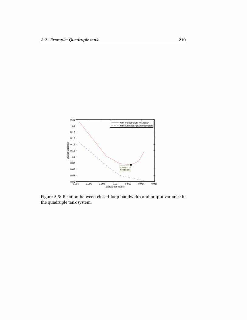
A.2. Example: Quadruple tank 219
0.004 0.006 0.008 0.01 0.012 0.014 0.0160.02
0.04
0.06
0.08
0.1
0.12
0.14
0.16
0.18
0.2
0.22
X: 0.01243Y: 0.07429
Bandwidth (rad/s)
Out
put v
aria
nce
With model−plant mismatchWithout model−plant mismatch
Figure A.6: Relation between closed-loop bandwidth and output variance inthe quadruple tank system.

220 Appendix to Chapter 2

BAppendix to Chapter 5
B.1 Proof of theorem 5.4.1
We show that r a nk ([ P Q ])≤ (2n+1)nd if Hp−H f < n+1. Assume Hp−H f <n +1, it implies that H f > n +1 since Hp ≥ 2(n +1). Note that
r a nk (([ P Q ]))
= r a nk ([ Hz N −Cz N C −1T u HT u CD C −1
T y HT y −HD ]). (B.1)
Let C −1T y =
I 0 0 0X1 I 0 0...
... I 0XHp−1 · · · X1 I
where Xk =−Tk −k−1∑
j=1Tk− j X j (Ford et al.
(2014)).Since
CD =
I 0 · · · · · · · · · · · · 0
D1...
......
......
......
...
Dn+1...
......
...
0...
......
......
......
......
... 00 · · · 0 Dn+1 · · · D1 I
, (B.2)

222 Appendix to Chapter 5
HT y =
T1 · · · Tn+1... ...
0
Tn+1 ... ...0 · · · 0...
...0 · · · 0
, (B.3)
and
HD =
D1 · · · Dn+1... ...
0
Dn+1 ... ...0 · · · 0...
...0 · · · 0
(B.4)
matrix CD C −1T y is:
I 0 · · · · · · · · · · · · 0
D1+X1 I...
...... D1+X1 I
......
Dn+1+Xn+1+n∑
i=1Di Xn+1−i
......
......
...
Xn+2+n+1∑
i=1Di Xn+2−i
......
......
...
......
...... 0
XHp−1+n+1∑
i=1Di XHp−1−i XHp
+n+1∑
i=1Di XHp−i · · · · · · · · · D1+X1 I
.
(B.5)
Therefore, matrix V :=CD C −1T y HT y −HD is:

B.1. Proof of theorem 5.4.1 223
T1 −D1 · · · Tn+1 −Dn+1(D1 +X1)T1 +T2 −D2 · · · (D1 +X1)Tn+1
(D2 +D1X1 +X2)T1 + (D1 +X1)T2 +T3 −D3 · · · (D2 +D1X1 +X2)Tn+1
......
...
(Dn +Xn +n−1∑
i=1Di Xn−i )T1 + . . .+ (D1 +X1)Tn +Tn+1 −Dn+1 · · · (Dn +Xn +
n−1∑
i=1Di Xn−i )Tn+1
(Dn+1 +Xn+1 +n∑
i=1Di Xn+1−i )T1 + . . .+ (D1 +X1)Tn+1 · · · (Dn+1 +Xn+1 +
n∑
i=1Di Xn+1−i )Tn+1
......
...
(XHp−1 +n+1∑
i=1Di XHp−1−i )T1 + . . .+ (D1 +X1)Tn+1 · · · (XHp−1 +
n+1∑
i=1Di XHp−1−i )Tn+1
.
Consider the first block column of V :
Vn+2;1 = (Dn+1+Xn+1+n∑
i=1
Di Xn+1−i )T1+ . . .+ (D1+X1)Tn+1. (B.6)
Substituting Xk =−Tk −k−1∑
j=1Tk− j X j into the coefficient of T1 in (B.6) gives:
Dn+1+Xn+1+n∑
i=1
Di Xn+1−i
=
Dn −Tn +n−1∑
i=1
X i (Dn−i −Tn−i )
T1
+
Dn−1−Tn−1+n−2∑
i=1
X i (Dn−1−i −Tn−1−i )
T2+ . . .+Dn+1−Tn+1 (B.7)
=−
(Dn +Xn +n−1∑
i=1
Di Xn−i )T1+ . . .+ (D1+X1)Tn +Tn+1−Dn+1
(B.8)
=Vn+1;1. (B.9)
Proceeding similarly, it follows that
Vn+2;1 =−n+1∑
i=1
Ti Vn+2−i ;1 (B.10)
and that
Vn+2; j =−n+1∑
i=1
Ti Vn+2−i ; j (B.11)

224 Appendix to Chapter 5
for 1 ≤ j ≤ n + 1. This relation shows the linear dependency of row n + 2 of Von rows 1; . . . ; n +1.
Note that
Vn+2;1 = Xn+2+n+1∑
i=1
Di Xn+2−i
=−Tn+2−n+1∑
j=1
Tn+2− j X j +n+1∑
i=1
Di Xn+2−i (B.12)
=Dn+1+Xn+1+n∑
i=1
Di Xn+1−i (B.13)
which is the coefficient of T1 in Vn+3;1.
Hence, by using the same calculation procedure, it can be derived that
Vk ; j =−k−1∑
i=1
Ti Vk−i ; j (B.14)
for n +2≤ k ≤Hp −1. This shows that from block row n +2, every block rowof V linearly depends on n +1 block rows above.
Now, the linear dependency of the rows of matrix W =Hz N −Cz N C −1T u HT u
is investigated. Note that
Cz N =
N1 0 · · · · · · 0...
......
...
Nn...
......
0...
... 0...
... Nn N1...
......
......
... Nn... 0...
...0 · · · · · · · · · 0
(B.15)
and

B.1. Proof of theorem 5.4.1 225
C −1T u =
I 0 0 0Z1 I 0 0...
... I 0ZH f −1 · · · Z1 I
(B.16)
Cz N C −1T u is:
N1 0 · · · · · · · · · · · · 0
N2+N1Z1 N1...
......
......
...
Nn +n−1∑
i=1Ni Zn−i Nn−1+
n−2∑
i=1Ni Zn−1−i · · · N1 0 · · · 0
n∑
i=1Ni Zn+1−i Nn +
n−1∑
i=1Ni Zn−i · · · · · · N1
......
...... 0
n∑
i=1Ni ZH f −i
n∑
i=1Ni ZH f −1−i · · · · · · · · · · · · N1
n∑
i=2Ni ZH f +1−i
n∑
i=2Ni ZH f −i · · · · · · · · · · · · N2
n∑
i=3Ni ZH f +2−i
n∑
i=3Ni ZH f +1−i · · · · · · · · · · · · N3
......
Nn ZH f −1 Nn ZH f −2 · · · · · · · · · · · · Nn
0 0 · · · · · · · · · · · · 0...
......
0 0 · · · · · · · · · · · · 0
(B.17)
With
HT u =
T1 · · · Tn+1... ...
0
Tn+1 ... ...0 · · · 0...
...0 · · · 0
(B.18)
and

226 Appendix to Chapter 5
Hz N =
N2 · · · Nn 0 0... ...
... ......
Nn ... ......
0 0 0...
......
0 · · · · · · 0 0
(B.19)
The first column of Hz N −Cz N C −1T u HT u is:
U =
N2−N1T1
N3− (N2+N1Z1)T1−N1T2...
−
n∑
i=1Ni Zn+1−i
T1− . . .−N1Tn+1
−
n∑
i=1Ni Zn+2−i
T1− . . .− (N2+N1Z1)Tn+1
...
−
n∑
i=1Ni ZH f −i
T1− . . .−
n∑
i=1Ni ZH f −n−i
Tn+1
−
n∑
i=2Ni ZH f +1−i
T1− . . .−
n∑
i=2Ni ZH f −n+1−i
Tn+1
...−(Nn ZH f −1)T1− . . .−Nn ZH f −n−1Tn+1
0...0
(B.20)
where Zk is assumed to be 0 for k < 0 and Z0 = I . We show that rows l of matrixU linearly depends on rows l −1; . . . ; l −n−1 for n+2≤ l ≤H f . The coefficientof T1 in row l of U is
n∑
i=1
Ni Zl−1−i (B.21)
=−n∑
i=1
Ni
l−2−i∑
j=0
Tl−1−i− j Z j
!
(B.22)
=
n∑
i=1
Ni Zl−2−i
T1+
n∑
i=1
Ni Zl−3−i
T2+ . . .+
n∑
i=1
Ni Zl−n−2−i
Tn+1 (B.23)

B.2. Proof of theorem 5.4.4 227
which is exactly row l − 1 of U . By using similar computation, the coefficientof T2 in row l of U is row l −2 of U , etc. and:
Ul =n+1∑
i=1
Ti Ul−i (B.24)
and this linear dependency also holds for other columns of Hz N −Cz N C −1T u HT u .
Hence, matrix
Γ =
Hz N −Cz N C −1T u HT u CD C −1
T y HT y −HD
(B.25)
satisfies
Γl ; j =n+1∑
i=1
Ti Γl−i ; j (B.26)
for n +2≤ l ≤H f .
Let PQs ho r t is the matrix formed with H f first rows of
P Q
and
[PQs ho r t ; PQr e s t ] =
P Q
.
Hence, r a nk (PQs ho r t )≤ n +1. Furthermore, if Hp −H f < n +1, PQr e s t has atmost n block rows and:
r a nk
P Q
≤ (r a nk (PQs ho r t )+n )nd ≤ (2n +1)nd (B.27)
and
P Q
is rank deficient.
B.2 Proof of theorem 5.4.4
r a nk
P Q R
= r a nk
Hz N −Cz N C −1T u HT u CD C −1
T y HT y −HD HF −CF C −1T d HT d
︸ ︷︷ ︸
M
. (B.28)
Note that matrix HF −CF C −1T d HT d has the same form as matrix
Hz N −Cz N C −1T u HT u . (B.29)
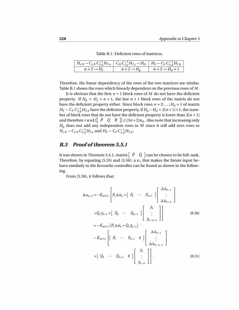
228 Appendix to Chapter 5
Table B.1: Deficient rows of matrices.
Hz N −Cz N C −1T u HT u CD C −1
T y HT y −HD HF −CF C −1T d HT d
n +2→H f n +2→Hp n +2→Hd +1
Therefore, the linear dependency of the rows of the two matrices are similar.Table B.1 shows the rows which linearly dependent on the previous rows of M .
It is obvious that the first n + 1 block rows of M do not have the deficientproperty. If Hp = H f + n + 1, the last n + 1 block rows of the matrix do nothave the deficient property either. Since block rows n + 2; . . . ; Hd + 1 of matrixHF −CF C −1
T d HT d have the deficient property, if Hp −Hd < 2(n+1)+1, the num-ber of block rows that do not have the deficient property is lower than 3(n +1)and therefore r a nk
P Q R
≤ (3n+2)nd . Also note that increasing onlyHp does not add any independent rows to M since it will add zero rows toHz N −Cz N C −1
T u HT u and HF −CF C −1T d HT d .
B.3 Proof of theorem 5.5.1
It was shown in Theorem 5.4.1, matrix
P Q
can be chosen to be full-rank.Therefore, by equating (5.55) and (5.56), a κ1 that makes the future input be-have similarly to the favourite controller can be found as shown in the follow-ing.
From (5.56), it follows that:
∆uk+1 =−KM P C
P1∆uk +
P2 · · · Pn+1
∆uk−1...
∆uk−n
+Q1 yk+1+
Q2 · · · Qn+1
yk...
yk−n+1
(B.30)
=−KM P C
P1∆uk +Q1 yk+1
− KM P C
P2 · · · Pn+1 0
∆uk−1...
∆uk−n−1
+
Q2 · · · Qn+1 0
yk...
yk−n
. (B.31)

B.3. Proof of theorem 5.5.1 229
By definition of T (z ),
∆uk =
I +T1z−1+ . . .+Tn+1z−n−1
∆uk . (B.32)
Therefore:
∆uk =∆uk −T1∆uk−1+ . . .+Tn+1∆uk−n−1. (B.33)
The definition of the open-loop system yields:
yk+1 =−D1 yk − . . .−Dn+1 yk−n
+N1∆uk + . . .+Nn∆uk−n+1. (B.34)
Substituting (B.33) and (B.34) into (B.31) yields:
∆uk+1 =−KM P C
P1∆uk −
T2 · · · Tn+2
∆ u←−k
−Q1
D1 · · · Dn+1
y←−k +Q1N1∆u (k )
+Q1
N2 · · · Nn 0 0
u←−k +
P2 · · · Pn+1 0
u←−k
+
Q2 · · · Qn+1 0
y←−k
. (B.35)
By substituting (B.33) and δuk =−KM P C
P u←−k +Q y←−k
into (B.35),
∆uk+1 = κ1∆u∆ u←−k +κ1y y←−k (B.36)
where κ1∆u and κ1y are given in (5.57) and (5.58), respectively. Hence, if κ1
satisfies −κ1
P Q
=
κ1∆u κ1y
,
∆u (k +1) =−κ1
P∆ u←−k +Q y←−k
(B.37)
will be equivalent to
∆u (k +1) =−KM P C
P∆ u←−k+1+Q y←−k+1
(B.38)
and the input sequence∆u (k ) and∆u (k + 1) will have the same behaviour asthe favourite controller in the unconstrained case.

230 Appendix to Chapter 5
Table B.2: Weighting matrixQne w (:, 1 : 10)divided by 100 in the case of no feed-forward control
178.4946 -1116.2399 478.8723 298.7760 -21.1279 92.4337 26.9939 105.0154 86.4808 -67.1654-1116.2399 -303.0324 -784.1438 193.7260 27.6128 242.4762 30.0181 30.9597 -18.2100 -44.4287
478.8723 -784.1438 3.2535 297.9746 23.0262 121.8910 27.7102 20.2198 23.9231 21.5680298.7760 193.7260 297.9746 58.5350 23.6008 -118.9841 -18.8126 81.6964 2.0610 -14.0016-21.1279 27.6128 23.0262 23.6008 -0.7440 -4.4702 -5.6286 -1.7073 -5.5189 2.079592.4337 242.4762 121.8910 -118.9841 -4.4702 -1.1724 -6.6821 -2.7327 -7.6830 -0.342726.9939 30.0181 27.7102 -18.8126 -5.6286 -6.6821 -5.5310 -3.9873 -13.6521 0.5162
105.0154 30.9597 20.2198 81.6964 -1.7073 -2.7327 -3.9873 -0.8666 -4.7853 -0.688786.4808 -18.2100 23.9231 2.0610 -5.5189 -7.6830 -13.6521 -4.7853 -8.5187 -0.2490-67.1654 -44.4287 21.5680 -14.0016 2.0795 -0.3427 0.5162 -0.6887 -0.2490 1.331891.1821 -9.1321 3.5679 -2.1602 -3.7775 -8.3829 -12.4372 -4.0865 -14.7489 1.073765.9322 -44.9896 6.9529 20.6235 4.9632 -1.5396 1.3626 1.3107 1.4218 2.18712.6098 1.5993 2.3868 2.2207 -1.2690 -8.4481 -9.6454 -4.8076 -13.5575 1.3255
63.7366 0.4587 22.0505 -9.2869 3.9073 -1.0017 2.6205 2.1854 0.8326 5.0575-58.1936 0.7410 5.6972 0.2703 4.0583 -7.7856 -4.8408 -2.7898 -5.0342 6.588864.2430 -6.1421 4.9071 14.5388 -3.1147 -4.7369 -10.0690 -4.4187 -13.0436 -0.3748-61.6709 7.8019 12.7974 4.1101 2.1043 -7.0148 -7.2048 -0.3851 -9.5911 6.095348.2837 13.5020 10.4700 -0.0197 -0.9476 -2.2740 -5.3517 -1.4608 -6.4348 1.511810.9550 10.6852 -2.4024 3.9199 2.4954 5.0965 7.1465 3.7256 10.1276 0.0838-26.8771 274.6695 4.6315 0.2907 0.1818 0.5911 -0.4164 -1.0716 1.5388 -0.2344-20.0185 -3.4657 -2.1673 -1.0279 -3.1136 -16.6007 -21.5451 -6.0699 -26.6409 2.5640-4.3679 -3.4037 20.8282 -6.6055 0.4065 -4.9783 -4.0147 -0.7599 -6.4552 4.97974.4600 -5.0562 -0.3957 0.1875 -5.6916 -8.2767 -13.0963 -6.7277 -14.7898 -1.5736
-112.4604 -15.8926 3.6911 -1.9078 -0.0899 -1.2979 -3.7569 -0.0653 -5.0217 1.3177-64.3998 32.2578 1.5029 0.2541 -2.3324 -7.1739 -10.8237 -3.8082 -13.3345 2.6373221.7828 -8.7361 19.8327 0.7166 -0.2257 -1.5684 -1.1844 -1.9421 -6.5043 0.9895-41.7516 -6.8784 23.8749 3.3848 -2.4615 -9.0577 -9.4549 -6.5711 -10.9874 -0.5927233.8458 -70.7921 144.3926 3.1835 0.2955 -3.0849 -4.0851 -0.8528 -6.5547 3.7403
B.4 Weighting matrices
B.4.1 Matching with no feed-forward control
The weighting matrices in the case of matching without feed-forward controlare given in Tables B.2,B.3,B.4,B.5 and B.6.
B.4.2 Matching with feed-forward control
The weighting matrices in the case of matching with feed-forward control aregiven in Tables B.7,B.8,B.9, B.10, B.11 and B.12.

B.4. Weighting matrices 231
Table B.3: Weighting matrix Qne w (:, 11 : 20) divided by 100 in the case of nofeed-forward control
91.1821 65.9322 2.6098 63.7366 -58.1936 64.2430 -61.6709 48.2837 10.9550 -26.8771-9.1321 -44.9896 1.5993 0.4587 0.7410 -6.1421 7.8019 13.5020 10.6852 274.66953.5679 6.9529 2.3868 22.0505 5.6972 4.9071 12.7974 10.4700 -2.4024 4.6315-2.1602 20.6235 2.2207 -9.2869 0.2703 14.5388 4.1101 -0.0197 3.9199 0.2907-3.7775 4.9632 -1.2690 3.9073 4.0583 -3.1147 2.1043 -0.9476 2.4954 0.1818-8.3829 -1.5396 -8.4481 -1.0017 -7.7856 -4.7369 -7.0148 -2.2740 5.0965 0.5911
-12.4372 1.3626 -9.6454 2.6205 -4.8408 -10.0690 -7.2048 -5.3517 7.1465 -0.4164-4.0865 1.3107 -4.8076 2.1854 -2.7898 -4.4187 -0.3851 -1.4608 3.7256 -1.0716
-14.7489 1.4218 -13.5575 0.8326 -5.0342 -13.0436 -9.5911 -6.4348 10.1276 1.53881.0737 2.1871 1.3255 5.0575 6.5888 -0.3748 6.0953 1.5118 0.0838 -0.2344-7.8841 3.1516 -12.9443 3.5806 -2.2494 -13.6691 -5.9271 -6.4564 6.3948 0.56643.1516 1.9313 6.0100 5.2795 8.6312 -0.1326 9.9048 3.5990 -2.8144 -1.6152
-12.9443 6.0100 -2.9208 4.4149 2.2094 -9.9387 -2.7582 -10.0827 6.4568 0.52293.5806 5.2795 4.4149 3.1231 8.1258 -1.0821 9.7498 2.0210 2.0607 1.5125-2.2494 8.6312 2.2094 8.1258 6.5329 -5.7143 11.4252 -7.0201 0.6668 -0.2868
-13.6691 -0.1326 -9.9387 -1.0821 -5.7143 -3.9061 -4.9163 -5.1994 8.7082 -0.1006-5.9271 9.9048 -2.7582 9.7498 11.4252 -4.9163 3.3074 -1.7814 3.1792 -0.8761-6.4564 3.5990 -10.0827 2.0210 -7.0201 -5.1994 -1.7814 -1.9664 6.2056 -0.16696.3948 -2.8144 6.4568 2.0607 0.6668 8.7082 3.1792 6.2056 -1.6857 -0.10530.5664 -1.6152 0.5229 1.5125 -0.2868 -0.1006 -0.8761 -0.1669 -0.1053 0.1418
-19.4132 9.5024 -16.6408 5.7906 2.3596 -20.1936 -1.5976 -19.8751 12.3349 2.0983-1.8343 6.7943 -5.4800 6.6030 4.0165 -6.5147 8.4819 2.1594 0.5187 -0.4227
-13.4226 0.5366 -10.4669 -0.2448 -4.3958 -12.7178 -5.9370 -11.7402 6.5438 0.1359-5.4456 0.5634 -2.9807 2.0612 -1.2726 -3.7214 1.5776 -2.3690 3.0564 1.7798
-10.2481 5.8065 -9.6743 4.6448 -1.0351 -9.2052 -0.9667 -6.0511 8.6572 0.7847-5.7214 1.8855 -1.8906 -0.3917 2.2482 -5.9388 5.0789 -4.6141 1.3796 0.4632-9.8804 2.3573 -7.2762 1.2213 1.9168 -12.8328 1.7123 -7.5925 5.9780 1.7876-4.5799 2.8193 -5.4641 3.4270 -0.3191 -2.8541 -4.0620 -0.6566 5.0021 -0.2243
Table B.4: Weighting matrix Qne w (:, 21 : 28) divided by 100 in the case of nofeed-forward control
-20.0185 -4.3679 4.4600 -112.4604 -64.3998 221.7828 -41.7516 233.8458-3.4657 -3.4037 -5.0562 -15.8926 32.2578 -8.7361 -6.8784 -70.7921-2.1673 20.8282 -0.3957 3.6911 1.5029 19.8327 23.8749 144.3926-1.0279 -6.6055 0.1875 -1.9078 0.2541 0.7166 3.3848 3.1835-3.1136 0.4065 -5.6916 -0.0899 -2.3324 -0.2257 -2.4615 0.2955
-16.6007 -4.9783 -8.2767 -1.2979 -7.1739 -1.5684 -9.0577 -3.0849-21.5451 -4.0147 -13.0963 -3.7569 -10.8237 -1.1844 -9.4549 -4.0851-6.0699 -0.7599 -6.7277 -0.0653 -3.8082 -1.9421 -6.5711 -0.8528
-26.6409 -6.4552 -14.7898 -5.0217 -13.3345 -6.5043 -10.9874 -6.55472.5640 4.9797 -1.5736 1.3177 2.6373 0.9895 -0.5927 3.7403
-19.4132 -1.8343 -13.4226 -5.4456 -10.2481 -5.7214 -9.8804 -4.57999.5024 6.7943 0.5366 0.5634 5.8065 1.8855 2.3573 2.8193
-16.6408 -5.4800 -10.4669 -2.9807 -9.6743 -1.8906 -7.2762 -5.46415.7906 6.6030 -0.2448 2.0612 4.6448 -0.3917 1.2213 3.42702.3596 4.0165 -4.3958 -1.2726 -1.0351 2.2482 1.9168 -0.3191
-20.1936 -6.5147 -12.7178 -3.7214 -9.2052 -5.9388 -12.8328 -2.8541-1.5976 8.4819 -5.9370 1.5776 -0.9667 5.0789 1.7123 -4.0620
-19.8751 2.1594 -11.7402 -2.3690 -6.0511 -4.6141 -7.5925 -0.656612.3349 0.5187 6.5438 3.0564 8.6572 1.3796 5.9780 5.00212.0983 -0.4227 0.1359 1.7798 0.7847 0.4632 1.7876 -0.2243
-19.9905 -9.2999 -22.3917 -7.8949 -20.3057 -5.5011 -10.0065 -4.8338-9.2999 2.5332 -11.0010 -2.4642 -3.8025 -3.6359 -11.7109 4.1192
-22.3917 -11.0010 -7.4309 -5.1027 -15.2969 -5.7937 -11.9360 -5.4973-7.8949 -2.4642 -5.1027 0.2227 -2.5724 -2.6997 -3.7492 0.8717
-20.3057 -3.8025 -15.2969 -2.5724 -3.6778 -2.5273 -6.2076 -0.9068-5.5011 -3.6359 -5.7937 -2.6997 -2.5273 -3.3553 -5.4471 -2.5170
-10.0065 -11.7109 -11.9360 -3.7492 -6.2076 -5.4471 -2.2799 -3.1901-4.8338 4.1192 -5.4973 0.8717 -0.9068 -2.5170 -3.1901 1.6034

232 Appendix to Chapter 5
Table B.5: Weighting matrix Rne w in the case of no feed-forward control
-1.9238 2.6527 -2.0015 2.84892.6527 -3.6724 2.6420 -3.7748-2.0015 2.6420 -2.0129 2.73032.8489 -3.7748 2.7303 -3.6895
Table B.6: Weighting matrix Sne w in the case of no feed-forward control
-187.7523 173.5567 -145.3176 94.4091239.0384 -349.7209 87.9873 -109.7501-160.9923 179.3315 -116.2592 103.9455-97.6305 134.6161 -33.8946 47.6467
4.1509 -8.9609 4.9461 -8.459618.6923 -21.3672 39.3366 -47.657654.9972 -72.5005 55.2557 -73.81721.6281 -6.3698 15.6400 -23.9870
66.4516 -84.6130 69.9184 -92.3576-9.6481 12.6886 -15.7540 19.579352.8778 -68.0849 55.9647 -74.5781-40.9516 54.3418 -32.8753 41.888647.7385 -62.0806 44.2146 -57.9400-37.1690 49.1996 -26.6868 34.1110-4.7214 4.8906 -9.5947 12.357755.8691 -73.8613 57.6154 -77.60851.7406 -8.7220 -2.9069 -1.1167
36.6332 -51.6890 39.6240 -56.4371-40.8541 52.4423 -35.4404 46.0687-12.6554 8.4627 -3.3639 4.901689.6427 -115.7987 79.2520 -102.656613.0326 -19.5255 11.7545 -18.455674.7293 -94.7389 68.3459 -87.385630.9706 -42.0919 18.0854 -24.338655.2143 -75.9933 46.3672 -63.5884-8.8970 14.3665 14.0889 -16.347242.5422 -51.3073 36.7004 -43.2670-27.7555 46.6538 1.2943 -2.8384

B.4. Weighting matrices 233
Table B.7: Weighting matrix Qne w (:, 1 : 10) in the case of feed-forward control
2135.8979 -1950.5736 -615.2862 -4066.5183 459.9833 -1002.1151 72.4131 574.5602 -172.6699 -457.5424-1950.5736 -4149.7862 -233.4435 97.3379 -165.1818 -2450.2669 -128.4429 -926.1413 65.8313 656.4916-615.2862 -233.4435 -2.4516 1.0608 -4.2751 -2.2180 -8.5966 -3.3199 -10.6380 -2.4017
-4066.5183 97.3379 1.0608 0.1951 1.8597 -0.5591 0.4259 0.6312 0.2819 0.7690459.9833 -165.1818 -4.2751 1.8597 -1.5921 -0.3026 -6.6485 -1.9970 -9.9031 -0.9152
-1002.1151 -2450.2669 -2.2180 -0.5591 -0.3026 -0.8734 -3.1975 -1.0680 -4.9390 -1.306672.4131 -128.4429 -8.5966 0.4259 -6.6485 -3.1975 -5.3523 -2.2608 -17.3821 -1.1905
574.5602 -926.1413 -3.3199 0.6312 -1.9970 -1.0680 -2.2608 -0.5393 -5.2292 0.7392-172.6699 65.8313 -10.6380 0.2819 -9.9031 -4.9390 -17.3821 -5.2292 -12.2729 -3.9780-457.5424 656.4916 -2.4017 0.7690 -0.9152 -1.3066 -1.1905 0.7392 -3.9780 1.3010-127.6155 29.9778 -10.5271 1.9878 -8.8952 -1.6293 -12.5185 -3.8985 -23.6582 -0.7075495.8916 89.4679 -5.5154 0.8854 -2.9591 -1.5598 -5.2777 -1.6025 -7.4644 0.004216.9090 14.1281 -13.7761 2.6090 -11.4549 -2.5547 -19.2486 -4.0301 -24.7185 1.4703
-390.8764 -27.2042 -2.0793 -1.0016 1.4809 -2.1397 0.4731 -1.0471 -4.1788 1.6396191.3171 -20.4928 -9.4660 3.9701 -5.6802 -5.3960 -9.5457 -3.9644 -19.4460 -2.7234-144.0444 239.3200 -4.1766 -1.1275 -2.5039 -1.8150 -1.9889 -1.2201 -7.1641 0.3573
15.4444 -13.4166 -13.4840 5.8603 -13.5319 -4.9587 -21.7582 -4.8326 -31.8770 -4.5976-588.4775 -396.4358 -3.0893 1.6180 -0.7199 -1.8199 -2.1433 -0.5982 -5.5114 1.0204-20.8992 22.8017 -9.3520 4.4707 -8.3942 -1.0709 -13.5655 -4.5240 -22.1443 1.0163
-333.0043 68.5071 -6.4108 0.2031 -3.3639 -4.1575 -9.0307 -1.9985 -13.4364 0.6935-32.5740 1.5275 -10.6669 -2.5595 -12.5318 -11.1281 -20.9415 -1.8284 -30.6351 -2.7220
-336.5210 5.0886 -4.0435 0.3344 0.5640 -1.5520 -3.8722 1.2650 -6.1966 2.802124.6651 0.0875 -15.3495 0.7124 -10.2610 -0.9352 -14.0635 -3.7769 -29.2917 1.3114
134.3354 15.5627 -1.3710 3.0933 3.5348 -0.8937 -0.4617 0.9903 -4.6623 5.6439-215.2659 69.0800 42.0666 -13.0817 39.0982 25.8710 60.1795 23.2206 96.6320 1.1308
40.2855 374.9432 14.5331 -2.8175 2.4062 7.5927 17.0517 1.2562 21.9346 -3.8998113.8493 19.6245 -41.7488 16.8472 -38.7071 -12.5819 -50.1544 -4.0841 -100.7518 10.5099-371.5827 -1.8984 -13.5139 2.2801 8.3659 -8.8518 -9.2915 -3.2684 -23.8878 5.2711
-6.6132 3.0799 3.9917 -1.1210 2.8776 -1.2167 3.0973 0.7009 5.5205 0.1609-148.7760 -15.7564 -0.3772 0.2662 -0.4331 0.2710 -0.5252 0.0447 -0.8665 0.2345300.7363 -20.4771 -7.1888 6.0474 -3.5172 -0.9397 -3.8854 -0.7671 -10.8539 2.9299-438.3174 105.5568 -3.5579 -2.4164 -0.8781 -6.5537 -5.3370 -6.7679 -7.5046 -6.0153-166.8998 37.9169 -3.8524 -2.7690 -3.8038 -7.4387 -10.0171 -4.8677 -14.3782 -2.5803568.4911 10.2584 3.2618 7.4350 -0.0388 6.7818 -4.6643 3.5688 -4.6356 10.6849
Table B.8: Weighting matrix Qne w (:, 11 : 20) in the case of feed-forward control
-127.6155 495.8916 16.9090 -390.8764 191.3171 -144.0444 15.4444 -588.4775 -20.8992 -333.004329.9778 89.4679 14.1281 -27.2042 -20.4928 239.3200 -13.4166 -396.4358 22.8017 68.5071-10.5271 -5.5154 -13.7761 -2.0793 -9.4660 -4.1766 -13.4840 -3.0893 -9.3520 -6.4108
1.9878 0.8854 2.6090 -1.0016 3.9701 -1.1275 5.8603 1.6180 4.4707 0.2031-8.8952 -2.9591 -11.4549 1.4809 -5.6802 -2.5039 -13.5319 -0.7199 -8.3942 -3.3639-1.6293 -1.5598 -2.5547 -2.1397 -5.3960 -1.8150 -4.9587 -1.8199 -1.0709 -4.1575
-12.5185 -5.2777 -19.2486 0.4731 -9.5457 -1.9889 -21.7582 -2.1433 -13.5655 -9.0307-3.8985 -1.6025 -4.0301 -1.0471 -3.9644 -1.2201 -4.8326 -0.5982 -4.5240 -1.9985
-23.6582 -7.4644 -24.7185 -4.1788 -19.4460 -7.1641 -31.8770 -5.5114 -22.1443 -13.4364-0.7075 0.0042 1.4703 1.6396 -2.7234 0.3573 -4.5976 1.0204 1.0163 0.6935
-10.2060 -6.6929 -22.1785 -2.3613 -14.1420 -6.5703 -28.2620 -3.1869 -11.5749 -10.4835-6.6929 -0.8755 -5.9073 -0.3164 -3.9415 -1.5745 -10.7014 0.1883 -1.2751 -3.6611
-22.1785 -5.9073 -11.4819 2.3703 -12.2346 -1.8261 -30.6765 -1.8215 -12.3377 -4.6602-2.3613 -0.3164 2.3703 0.3590 0.7897 -1.0991 -3.5636 0.7891 7.1300 -0.7740
-14.1420 -3.9415 -12.2346 0.7897 -3.2613 -4.4630 -20.8945 -3.4280 -2.4988 -10.7066-6.5703 -1.5745 -1.8261 -1.0991 -4.4630 -2.0384 -10.1474 -0.4909 -1.7179 -3.0747
-28.2620 -10.7014 -30.6765 -3.5636 -20.8945 -10.1474 -21.6932 -11.3379 -23.8680 -19.0024-3.1869 0.1883 -1.8215 0.7891 -3.4280 -0.4909 -11.3379 1.0773 0.0962 0.1309
-11.5749 -1.2751 -12.3377 7.1300 -2.4988 -1.7179 -23.8680 0.0962 -2.4158 -0.1726-10.4835 -3.6611 -4.6602 -0.7740 -10.7066 -3.0747 -19.0024 0.1309 -0.1726 -1.3777-24.9747 -8.8023 -28.3061 0.3321 -16.2726 -7.4859 -33.9089 -3.3496 -25.7811 -18.2901-3.2392 -2.6353 1.3848 0.1929 -6.0684 -2.8661 -8.6179 2.0081 2.3668 -2.3649
-20.1046 -3.4583 -19.2838 -1.4112 -5.8355 -5.0808 -26.8931 -3.7558 -16.5383 -4.49371.7255 1.9018 6.2624 2.6927 6.5541 0.1329 -3.9550 1.8887 7.1238 -1.9010
89.3110 24.7822 77.4794 -3.4379 51.7088 10.0792 129.2871 13.3965 51.9936 37.625920.1525 3.4922 3.6269 1.9151 6.6071 6.8049 24.1158 5.6703 -3.0914 7.5258-96.2681 -11.1051 -95.3710 9.3915 -41.9343 2.7946 -153.2811 -2.5667 -60.7898 -23.7781
1.9248 -1.2986 3.1692 10.2289 -4.9170 -6.6926 -20.2395 7.0143 19.1946 1.00175.8105 2.4269 6.6480 -0.2155 3.3052 0.5879 8.0603 0.3864 4.3871 2.2481-0.7924 0.2286 -0.8621 0.5915 -0.3389 0.5243 -1.1931 0.5838 -0.5565 0.3978
-14.5415 -5.3362 -14.0030 2.3879 -7.2954 -0.6986 -17.9516 2.6468 -7.1461 -0.3196-6.7530 -8.9889 -5.5378 -8.9376 -5.2355 -10.9294 -14.3777 -8.6449 -3.4828 -12.2383-9.6333 -8.3899 -6.7749 -2.8465 -2.9619 -5.7092 -16.5227 -3.2396 -6.9052 -6.27204.5824 5.3789 12.7863 7.1923 7.8043 6.4084 3.4666 9.3533 9.5489 8.3810

234 Appendix to Chapter 5
Table B.9: Weighting matrix Qne w (:, 21 : 30) in the case of feed-forward control
-32.5740 -336.5210 24.6651 134.3354 -215.2659 40.2855 113.8493 -371.5827 -6.6132 -148.77601.5275 5.0886 0.0875 15.5627 69.0800 374.9432 19.6245 -1.8984 3.0799 -15.7564
-10.6669 -4.0435 -15.3495 -1.3710 42.0666 14.5331 -41.7488 -13.5139 3.9917 -0.3772-2.5595 0.3344 0.7124 3.0933 -13.0817 -2.8175 16.8472 2.2801 -1.1210 0.2662
-12.5318 0.5640 -10.2610 3.5348 39.0982 2.4062 -38.7071 8.3659 2.8776 -0.4331-11.1281 -1.5520 -0.9352 -0.8937 25.8710 7.5927 -12.5819 -8.8518 -1.2167 0.2710-20.9415 -3.8722 -14.0635 -0.4617 60.1795 17.0517 -50.1544 -9.2915 3.0973 -0.5252-1.8284 1.2650 -3.7769 0.9903 23.2206 1.2562 -4.0841 -3.2684 0.7009 0.0447
-30.6351 -6.1966 -29.2917 -4.6623 96.6320 21.9346 -100.7518 -23.8878 5.5205 -0.8665-2.7220 2.8021 1.3114 5.6439 1.1308 -3.8998 10.5099 5.2711 0.1609 0.2345
-24.9747 -3.2392 -20.1046 1.7255 89.3110 20.1525 -96.2681 1.9248 5.8105 -0.7924-8.8023 -2.6353 -3.4583 1.9018 24.7822 3.4922 -11.1051 -1.2986 2.4269 0.2286
-28.3061 1.3848 -19.2838 6.2624 77.4794 3.6269 -95.3710 3.1692 6.6480 -0.86210.3321 0.1929 -1.4112 2.6927 -3.4379 1.9151 9.3915 10.2289 -0.2155 0.5915
-16.2726 -6.0684 -5.8355 6.5541 51.7088 6.6071 -41.9343 -4.9170 3.3052 -0.3389-7.4859 -2.8661 -5.0808 0.1329 10.0792 6.8049 2.7946 -6.6926 0.5879 0.5243
-33.9089 -8.6179 -26.8931 -3.9550 129.2871 24.1158 -153.2811 -20.2395 8.0603 -1.1931-3.3496 2.0081 -3.7558 1.8887 13.3965 5.6703 -2.5667 7.0143 0.3864 0.5838
-25.7811 2.3668 -16.5383 7.1238 51.9936 -3.0914 -60.7898 19.1946 4.3871 -0.5565-18.2901 -2.3649 -4.4937 -1.9010 37.6259 7.5258 -23.7781 1.0017 2.2481 0.3978-22.7702 -9.2077 -31.8419 2.0672 108.7260 17.0835 -106.3132 -18.2667 6.7123 -0.8583-9.2077 -0.5892 -2.0834 -1.1477 27.1316 3.7829 2.9596 7.1856 -0.7948 0.7679
-31.8419 -2.0834 -10.4566 7.3890 61.3643 12.8576 -114.3986 2.8458 4.1161 -0.57692.0672 -1.1477 7.3890 2.7276 -11.2827 -7.3990 38.6012 16.9158 -1.4631 1.0237
108.7260 27.1316 61.3643 -11.2827 -148.1397 -79.8042 327.8295 49.6662 -12.6091 3.478417.0835 3.7829 12.8576 -7.3990 -79.8042 -12.6545 31.3479 16.0180 -0.0830 -2.0937
-106.3132 2.9596 -114.3986 38.6012 327.8295 31.3479 -190.1519 -28.3893 14.8784 -3.3427-18.2667 7.1856 2.8458 16.9158 49.6662 16.0180 -28.3893 -2.6441 -6.3705 3.2280
6.7123 -0.7948 4.1161 -1.4631 -12.6091 -0.0830 14.8784 -6.3705 -0.3514 0.4031-0.8583 0.7679 -0.5769 1.0237 3.4784 -2.0937 -3.3427 3.2280 0.4031 -0.0423
-11.7976 2.9838 -3.6383 9.6908 58.0668 6.5401 -46.5667 22.4210 3.8856 -0.4408-13.0219 -12.0951 -9.0107 -11.7820 22.4438 31.6830 -38.5744 -37.1385 -0.3754 0.6401-13.6793 0.5763 -7.7450 2.9038 44.9340 9.0455 -54.1917 8.6697 2.1890 -0.2462
8.2235 9.4923 9.0563 13.7181 -4.4140 -25.5306 7.5291 43.1162 1.9883 0.3803
Table B.10: Weighting matrixQne w (:, 31 : 34) in the case of feed-forward control
300.7363 -438.3174 -166.8998 568.4911-20.4771 105.5568 37.9169 10.2584-7.1888 -3.5579 -3.8524 3.26186.0474 -2.4164 -2.7690 7.4350-3.5172 -0.8781 -3.8038 -0.0388-0.9397 -6.5537 -7.4387 6.7818-3.8854 -5.3370 -10.0171 -4.6643-0.7671 -6.7679 -4.8677 3.5688
-10.8539 -7.5046 -14.3782 -4.63562.9299 -6.0153 -2.5803 10.6849
-14.5415 -6.7530 -9.6333 4.5824-5.3362 -8.9889 -8.3899 5.3789
-14.0030 -5.5378 -6.7749 12.78632.3879 -8.9376 -2.8465 7.1923-7.2954 -5.2355 -2.9619 7.8043-0.6986 -10.9294 -5.7092 6.4084
-17.9516 -14.3777 -16.5227 3.46662.6468 -8.6449 -3.2396 9.3533-7.1461 -3.4828 -6.9052 9.5489-0.3196 -12.2383 -6.2720 8.3810
-11.7976 -13.0219 -13.6793 8.22352.9838 -12.0951 0.5763 9.4923-3.6383 -9.0107 -7.7450 9.05639.6908 -11.7820 2.9038 13.7181
58.0668 22.4438 44.9340 -4.41406.5401 31.6830 9.0455 -25.5306
-46.5667 -38.5744 -54.1917 7.529122.4210 -37.1385 8.6697 43.11623.8856 -0.3754 2.1890 1.9883-0.4408 0.6401 -0.2462 0.3803-1.7186 -1.6928 -9.1127 8.1106-1.6928 -8.3569 -8.2780 -0.2586-9.1127 -8.2780 -2.2100 3.23818.1106 -0.2586 3.2381 7.4293

B.4. Weighting matrices 235
Table B.11: Weighting matrix Rne w in the case of feed-forward control
-0.9581 1.36881.3688 -1.9564
Table B.12: Weighting matrix Sne w in the case of feed-forward control
2.9958 6.618410.5362 -9.23573.3157 -4.57853.0580 -4.69721.6635 -2.47083.1270 -3.59943.3154 -4.62880.6004 -0.49526.0396 -8.5440-0.1191 -0.16695.1771 -7.56920.5907 -0.85104.6326 -6.9384-0.0002 -0.08682.4716 -3.55060.5794 -0.80307.9081 -11.29891.1567 -1.62752.8456 -4.50602.1017 -3.09046.2630 -8.95840.8819 -1.34514.8229 -7.1187-1.6980 2.2847
-15.7421 22.0729-3.3433 4.588315.3966 -22.51652.0486 -3.0568-0.7878 1.21970.2715 -0.44662.1457 -3.40202.8775 -3.69372.7757 -4.1431-1.9009 2.1576

236 Appendix to Chapter 5
CAppendix to Chapter 6
C.1 Proof of theorem 6.3.1
N∑
l=0
cos
2π
N +1l p +φ
= Re
N∑
l=0
e j ( 2πN+1 l p+φ)
(C.1)
(C.2)
Using the equality
n∑
k=0
a k = (a n+1−1)/(a −1), ∀a 6= 1 (C.3)
we derive that, if p 6= k (N +1), ∀k ∈Z (i.e. e j 2πN+1 p 6= 1):
Re
N∑
l=0
e j ( 2πN+1 l p+φ)
= Re
e jφ e j 2πN+1 (N+1)p −1
e j 2πN+1 p −1
(C.4)
= 0 (Q.E.D)

238 Appendix to Chapter 6
C.2 Proof of theorem 6.3.2
First we prove that ‖v Nl ‖2 = 1 for 1≤ l ≤N . ‖v N
l ‖2 is the square root of:
1
L 2
N∑
k=1
cos2 π
N +1k l +ϕl
=1
2L 2
N∑
k=1
1+ cos
2π
N +1k l +2ϕl
(C.5)
=1
2L 2
N +N∑
k=1
cos
2π
N +1k l +2ϕl
(C.6)
=1
2L 2
N − cos
2ϕl
+N∑
k=0
cos
2π
N +1k l +2ϕl
(C.7)
= 1 (C.8)
thanks to Theorem 6.3.1 and L =q
N − cos
2ϕl
/2.Now, we prove that (6.31) holds for v N
l using the same reasoning as in Sec-tion 6 of Rojas et al. (2004). Consider the energy density spectrum of the sys-tem, which is the Discrete Time Fourier Transform (DTFT) of the autocorrela-tion sequence of the impulse response:
Φ(ω) =∞∑
l=−∞φl e − jωl ,ω= [−π,π] (C.9)
where
φl =k0−l∑
k=0
Mk Mk+l for 0≤ l ≤ k0 (C.10)
φl ≈ 0 for l > k0 (C.11)
φ−l =φl (C.12)
The energy density spectrum is also computed as follows:
Φ(ω) =k0∑
l=−k0
φl e − jωl (C.13)

C.3. Proof of theorem 6.3.3 239
=φ0+2k0∑
l=1
φl cos(ωl ),ω= [−π,π] (C.14)
The Hessian matrix is H= T >T (considering Q = I and R = 0):
HN =
X1 | 0φ−k0
. . . φ0 . . . φk00 . . . 0
0...
......
......
......
... 00 · · · 0 φ−k0
. . . φ0 . . . φk0
0 | X2
(C.15)
where X1 and X2 are suitable matrices. Using the trigonometric identity
cosα+ cosβ = 2(cosα+β
2+ cos
α−β2) for α,β ∈R (C.16)
and the fact that φl = φ−l for 0 ≤ l ≤ k0 to calculate HN0v N0
l0with N0 > 0, 0 ≤
l0 ≤N0−1 and v N0l0
given by (6.35), we also obtain
HN0v N0
l0=
c1
Φ(ω0)vN0l0(k0+1 : N0−k0)
c2
(C.17)
where c1 and c2 are suitable column vectors of length k0 and v N0l0(k0+1 : N0−k0)
is the vector formed by the elements of v N0l0
in (6.35), from k0+1 to N0−k0.The rest of the proof is similar to that in Rojas et al. (2004). To conclude,
vector v Nl is the right singular vector of the Toeplitz matrix.
C.3 Proof of theorem 6.3.3
From Subsection 6.2.2, it follows that the magnitude of the frequency responseis given by the singular values of the Toeplitz matrix. Using the properties ofSVD, we obtain:
T Vn = |G (e jωn )|Un ⇒ V >n T Vn = |G (e jωn )|V >n Un (C.18)

240 Appendix to Chapter 6
The term V >n T Vn can be computed from (6.4) and (6.39):
V >n T Vn =k0∑
m=0
1
L 2
N−m∑
l=1
cos π
N +1l n +ϕn
cos π
N +1(l +m )n +ϕn
Mm
(C.19)
=k0∑
m=0
Am Mm (C.20)
The asymptotic values of the factors Am are computed using the trigono-metric identity
cosαcosβ =1
2
cos(α+β ) + cos(α−β )
(C.21)
It follows that, with m = 0, 1, . . . , k0:
Am =2
N − cos
2ϕn
N−m∑
l=1
h
cos π
N +1l n +ϕn
cos π
N +1(l +m )n +ϕn
i
(C.22)
=1
N − cos
2ϕn
N−m∑
l=1
h
cos π
N +1(2l +m )n +2ϕn
+ cos π
N +1mn
i
(C.23)
=N −m
N − cos
2ϕn
cos π
N +1mn
+1
N − cos
2ϕn
N∑
l=1
cos π
N +1(2l +m )n +2ϕn
−1
N − cos
2ϕn
N∑
l=N−m+1
cos π
N +1(2l +m )n +2ϕn
(C.24)
From Theorem 6.3.1, it implies that:
1
N − cos
2ϕn
N∑
l=0
cos π
N +1(2l +m )n +2ϕn
= 0. (C.25)
Therefore
1
N − cos
2ϕn
N∑
l=1
cos π
N +1(2l +m )n +2ϕn
→ 0 when N →∞. (C.26)
In addition, it is obvious that

C.4. Proof of theorem 6.3.4 241
−m
N − cos
2ϕn
≤1
N − cos
2ϕn
N∑
l=N−m+1
cos π
N(2l +m )n +2ϕn
≤m
N − cos
2ϕn
hence:
1
N − cos
2ϕn
N∑
l=N−m+1
cos π
N +1(2l +m )n +2ϕn
→ 0 when N →∞. (C.27)
From (C.24), (C.26), and (C.27), we obtain the asymptotic value of Am , whenN →∞:
Am →N −m
N − cos
2ϕn
cos π
N +1mn
→ cos π
N +1mn
(C.28)
From (C.28), it implies that Am → cos
πN mn
when N →∞. Using (C.20), wederive that, when N →∞:
V >n T Vn =k0∑
m=0
cos π
N +1mn
Mm (C.29)
=Re
k0∑
m=0
e − jωn m Mm
!
withωn =π
N +1n (C.30)
=Re
G (e jωn )
(C.31)
This is the real part of the frequency response of the system at frequency ωn .From (C.18) and (C.31), it implies that:
|G (e jωn )|V >n Un =Re(G (e jωn )) (C.32)
⇒V >n Un = cos
a r g (G (e jωn ))
(C.33)
We notice that V >n Un is scalar and (V >n Un )> =U >n Vn . This completes the proof.
C.4 Proof of theorem 6.3.4
From the relation between the gain of the system and the singular values of theToeplitz matrix described above and (6.43), it follows that

242 Appendix to Chapter 6
T Vi ,p =σi (ω)Ui ,p (C.34)
⇒V >i ,p
T Vi ,p =σi (ω)V>
i ,pUi ,p (C.35)
where T is given in (6.50) and Vi ,p in (6.46). Using theorem 6.3.1 and the trigono-metric identity:
cos x cos y =1
2(cos(x + y )cos(x − y )) for x ; y ∈R (C.36)
after some calculations similar to the proof of Theorem 6.3.3, we obtain
V >i ,p
T Vi ,p =Re
1
N −1
e − jωv∗G i e − j 2ωv∗G i · · · e − j Nωv∗G i
T
e jωvG i
e j 2ωvG i
...e j NωvG i
(C.37)
=Re
1
N −1
N v∗G i M0vG i + (N −1)v∗G i e − jωM1vG i + · · ·+ (N −k0)v∗G i e − jωk0 Mk0
vG i
=Re
N
N −1v∗G i M0vG i +v
∗G i e − jωM1vG i + · · ·+
N −k0
N −1v∗G i e − jωk0 Mk0
vG i
(C.38)
In the limit N →∞, N−kN−1 → 0 with a constant k . Hence, the equality above
leads to
V >i ,p
T Vi ,p =Re
v∗G i
k0∑
l=0
e − jωl Ml
!
vG i
!
(C.39)
=Re
v>G i G (e jω)vG i
⇒Re
V >i ,p
T Vi ,p
=Re
(v∗G i G (e jω)vG i )
(C.40)
On the other hand, we have
G (e jω)vG i =σi (ω)uG i (C.41)
⇒ v∗G i G (e jω)vG i =σi (ω)v∗G iuG i (C.42)
=σi cosφ(i ,ω)e j∆θ (i ,ω) (C.43)
⇒Re
v∗G i G (e jω)vG i
=σi cos
φ(i ,ω)
cos (∆θ (i ,ω)) (C.44)
From (C.35), (C.40) and (C.44), it follows that
U >i ,p Vi ,p = cos
φ(i ,ω)
cos (∆θ (i ,ω)) (C.45)
(Q.E.D)

C.5. Proof of theorem 6.3.5 243
C.5 Proof of theorem 6.3.5
By definition, the i t h row of matrix H xp a s t +T x f u t u r e is given by
M0 cos
iω+ϕ
+M1 cos
(i −1)ω+ϕ
+ . . .+Mi−1 cos
ω+ϕ
+Mi cosϕ+Mi+1 cos
−ω+ϕ
+ . . .+MNp a s tcos
i −Np a s t
ω+ϕ
=Np a s t∑
j=0
M j cos
i − j
ω+ϕ
=Re
Np a s t∑
j=0
M j e (i− j )ω+ϕ!
=Re
e iω+ϕNp a s t∑
j=0
M j e − jω
!
=Re
σωe iω+ϕ+ϕω
=σω cos
iω+ϕ+ϕω
. (C.46)
This equality directly leads to the result of the theorem.
C.6 Proof of theorem 6.3.7
Consider 2 column vectors yf u t u r e
i and yf u t u r e
j (i 6= j )of Yf u t u r e . By con-struction:
yf u t u r e
i
>y
f u t u r ej =
N∑
k=1
cos
kωi +π
2
cos
kω j +π
2
=1
2
N∑
k=1
cos
kπ
i − j
N +1
−N∑
k=1
cos
kπ
i + j
N +1
(C.47)
If i − j = 2l where l ∈Z,
N∑
k=1
cos
kπ
i − j
N +1
= 1−N∑
k=0
cos
2kπl
N +1
= 1 (C.48)
due to Theorem 6.3.1. Similarly

244 Appendix to Chapter 6
N∑
k=1
cos
kπ
i + j
N +1
= 1−N∑
k=0
cos
2kπ(l + j )N +1
= 1 (C.49)
and therefore
yf u t u r e
i
>y
f u t u r ej = 1−1= 0.
If i − j = 2l +1 where l ∈Z and N +1 is even:
N∑
k=1
cos
kπ
i − j
N +1
=N∑
k=1
cos
kπ(2l +1)N +1
= cos(N +1)π(2l +1)
2 (N +1)+
N+12∑
k=1
cos
kπ(2l +1)N +1
+ cos (N +1−k )π(2l +1)
N +1
= 0+0= 0(C.50)
and similarlyN∑
k=1cos
kπ(i+ j )N+1
= 0. Hence
yf u t u r e
i
>y
f u t u r ej = 1−1= 0.
If i − j = 2l +1 where l ∈Z and N +1 is odd:
N∑
k=1
cos
kπ
i − j
N +1
=N∑
k=1
cos
kπ(2l +1)N +1
=
N2∑
k=1
cos
kπ(2l +1)N +1
+ cos (N +1−k )π(2l +1)
N +1
= 0
(C.51)
and similarlyN∑
k=1cos
kπ(i+ j )N+1
= 0. Hence
yf u t u r e
i
>y
f u t u r ej = 1− 1 = 0 and
matrix Yf u t u r e is orthogonal.
The square of the length of a column vector yf u t u r e
i is given by:
N∑
k=1
cos2
kωi +π
2
=N
2+
1
2
N∑
k=1
cos (2kωi +π)
=N
2−
1
2
N∑
k=1
cos
2kπi
N +1
=N +1
2
(C.52)

C.6. Proof of theorem 6.3.7 245
according to Theorem 6.3.1. Therefore, the length of yf u t u r e
i is a constant anddoes not depend on i . (Q.E.D)

246 Appendix to Chapter 6

Acknowledgements
First of all, I would like to express my very great appreciation to Professor TonBackx, my promoter, and Dr. Leyla Özkan, my daily supervisor, for giving methe opportunity to conduct the fascinating research on the tuning of model-based controllers, and for your constant guidance and encouragement through-out the undertaking of my research. Thanks also to Dr. Jobert Ludlage for shar-ing your inspiring ideas and extensive knowledge of the field of process control.
I am very grateful to the members of my dissertation committee. ProfessorJan Maciejowski, Professor Alf Isaksson, Professor Paul Van den Hof, Dr. Tonvan den Boom and Dr. Federico Felici, thank you for your efforts to read mythesis and for your invaluable feedback. I would also like to thank ProfessorAarnout Brombacher for his willingness to chair the dissertation committee.
I also owe a great deal to the industrial partners in the Autoprofit project.I wish to thank Dr. Per Erik Modén and Dr. Michael Lundh from ABB Corpo-rate Research for their useful support and discussions throughout the project.I would also like to thank Hernan Guidi and Ollie Olwagen from SASOL Ltd forhelping me carry out my experiments on SASOL’s simulator and actual distilla-tion column. Thanks also to the partners from Boliden for giving me the insightinto Boliden’s floatation plant and the opportunity to visit Boliden’s site.
My grateful thanks are also extended to the academic partners in the Au-toprofit project for the useful discussions we had. I also wish to acknowledgethe contribution of the Master’s and Bachelor students to my research. In ad-dition, I would also like to thank Barbara Cornelissen - Milner, our secretary,Will Hendrix and Udo Bartzke, the technical assistants, for their help.
Finally, I would like to express my deep gratitude to my parents for their

248 Appendix to Chapter 6
unfailing support and encouragement throughout my PhD project. This thesisis dedicated to them.

Curriculum Vitae
Tran Nhat Quang was born on 12 December 1986 in Hanoi, Vietnam. He re-ceived his M.Sc. and M.Eng. degrees in Electrical Engineering from the Greno-ble Institute of Technology (Grenoble INP), Grenoble, France, in 2010. In hisgraduation project, he studied the complex dynamics of a combustion enginemodel developed by Renault. Then he investigated different optimisation meth-ods to identify the parameters of the model using grey-box identification tech-niques. The engine model was subsequently used by Renault to design futureengines which meet EURO 6 standards.
In November 2010, Tran Nhat Quang started his PhD at the Control Systemsgroup in the Department of Electrical Engineering of Eindhoven University ofTechnology. This PhD was undertaken in the AUTOPROFIT project, whose aimwas to develop autonomous maintenance technologies for model-based oper-ations support systems. During his M.Sc. and PhD projects, Quang Tran hasdeveloped his research interests in process control, model predictive control,robust control and modelling.