Tunable molecular resonances of a double quantum dot Aharonov–Bohm interferometer

This article has been downloaded from IOPscience. Please scroll down to see the full text article.

2004 J. Phys.: Condens. Matter 16 117

(http://iopscience.iop.org/0953-8984/16/1/011)

Download details:

IP Address: 129.15.14.53

The article was downloaded on 01/09/2013 at 19:34

Please note that terms and conditions apply.

View the table of contents for this issue, or go to the journal homepage for more

Home Search Collections Journals About Contact us My IOPscience

INSTITUTE OF PHYSICS PUBLISHING JOURNAL OF PHYSICS: CONDENSED MATTER

J. Phys.: Condens. Matter 16 (2004) 117–124 PII: S0953-8984(04)69121-1

Tunable molecular resonances of a double quantumdot Aharonov–Bohm interferometer

Kicheon Kang1 and Sam Young Cho2

1 Department of Physics, Chonnam National University, Gwangju 500-757, Korea2 Department of Physics, University of Queensland, Brisbane 4072, Australia

Received 17 September 2003Published 15 December 2003Online at stacks.iop.org/JPhysCM/16/117 (DOI: 10.1088/0953-8984/16/1/011)

AbstractWe investigate resonant tunnelling through molecular states of an Aharonov–Bohm (AB) interferometer composed of two coupled quantum dots. Theconductance of the system shows two resonances associated with the bondingand the antibonding quantum states. We predict that the two resonances arecomposed of a Breit–Wigner resonance and a Fano resonance, of which thewidths and Fano factor depend on the AB phase very sensitively. Further, wepoint out that the bonding properties, such as the covalent and ionic bonding,can be identified by the AB oscillations.

(Some figures in this article are in colour only in the electronic version)

While single quantum dots are regarded as artificial atoms due to their quantization ofenergies [1, 2], two (or more) quantum dots can be coupled to form an artificial molecule [3].Resonant tunnelling through serially coupled quantum dots provides some information on thecoupling between dots [4], but the phase coherence of the bonding cannot be directly addressedin this geometry. Aharonov–Bohm (AB) interferometers containing a quantum dot in one ofthe two arms enables the investigation of the phase coherent transmission through a quantumdot [5–7]. The phase coherence of the Kondo-assisted transmission has also been studied inthis geometry [8–14]. Recently, an AB interferometer set-up containing two coupled quantumdots has been realized [15]. This can be considered as the beginning point in the study ofthe experimentally unexplored region where various aspects of a double dot molecule can beinvestigated by probing the phase coherence. There are some previous theoretical works on theAB interferometer containing two quantum dots. Resonant tunnelling [16], cotunnelling [17],Kondo effect [18] and magnetic polarization current [19] have been the topics of study of thesystem in the absence of direct coupling between the two dots. Two-electron entanglementin the presence of direct tunnelling between the dots has also been studied [20] in relation toquantum communication.

In this paper, we study phase-sensitive molecular resonances in an Aharonov–Bohminterferometer made of two coupled quantum dots. The geometry we consider is schematicallydrawn in figure 1 and is equivalent to the experimental set-up of [15]. We find that the

0953-8984/04/010117+08$30.00 © 2004 IOP Publishing Ltd Printed in the UK 117

118 K Kang and S Y Cho

B

RL

ε

ε 2

1

V

V

t

V

V

Figure 1. Schematic diagram of double quantum dots embedded in an Aharonov–Bohminterferometer.

conductance of the system consists of two molecular resonances, associated with the bondingand the antibonding quantum states. By careful analysis of the conductance as a function ofenergy, we argue that the two resonances are always composed of a Breit–Wigner resonanceand a Fano resonance, with those widths and Fano factor depending very sensitively on theAB phase. Further, we point out that the bonding properties, such as the covalent and ionicbonding, can be characterized by the AB oscillations.

Our model is described by the following Hamiltonian:

H = HM + H0 + HT, (1a)

where HM, H0 and HT stand for the artificial molecules of double quantum dots, two electricalleads and tunnelling between the leads and the quantum dots, respectively. For the molecule,we consider coupled non-interacting quantum dots of energies ε1, ε2 with a tunnelling matrixelement t between them:

HM = ε1d†1 d1 + ε2d†

2 d2 − t (d†1 d2 + d†

2 d1), (1b)

where di (d†i ) with i = 1, 2 annihilates (creates) an electron in the i th dot. The bonding

properties depend on the ratio of the energy difference of the quantum dot levels (�ε ≡ ε1−ε2)and the level splitting due to tunnelling (2t). The molecular bonding can be called ‘covalent’for |�ε| � 2t , where the eigenstates of the electrons are delocalized. On the other hand, themolecule is considered to be in the ‘ionic’ bonding limit for |�ε| � 2t , where the eigenstatesare localized in one of the two dots [3]. H0 describes the two (left and right) electrical leadsmodelled by the Fermi sea as

H0 =∑

k∈L

ELk a†

k ak +∑

k∈R

ERk b†

kbk, (1c)

where ak (a†k ) and bk (b†

k ) annihilates (creates) an electron in the left and one in the rightleads, respectively. These two leads are assumed to be identical (Ek ≡ EL

k = ERk ). Finally,

tunnelling between the leads and the molecule is described by

HT = −∑

k,i=1,2

(V iLd†

i ak + H.c.) −∑

k,i=1,2

(V iRd†

i bk + H.c.). (1d)

For simplicity, we assume that the magnitudes of the tunnelling matrix elements of the fourdifferent arms are the same (denoted by V ). Then the matrix elements can be written asV 1

L = V 2R = V eiϕ/4, V 2

L = V 1R = V e−iϕ/4. ϕ represents the AB phase defined as ϕ = 2π�/�0

where � and �0 are the external flux through the interferometer and the flux quantum (=hc/e),respectively. The hopping strength between a quantum dot and a lead is denoted by �, definedas

� = 2πρ(EF)V 2, (2)

where ρ(EF) stands for the density of states of each lead at the Fermi level, EF.

Tunable molecular resonances of a double quantum dot Aharonov–Bohm interferometer 119

The Hamiltonian is transformed by using the symmetric and antisymmetric modes of theleads and the quantum dots. Below it will become obvious that this approach provides betterinsights into the problem. Let us consider the transformations of electron operators:

αk = (ak + bk)/√

2, βk = (ak − bk)/√

2, (3a)

dα = (d1 + d2)/√

2, dβ = i(d1 − d2)/√

2. (3b)

Note that, for ε1 = ε2, dα and dβ correspond to the annihilation operator of the bonding andthe antibonding modes. By adopting this transformation we can rewrite the Hamiltonian asfollows:

H = Hα + Hβ + Hαβ, (4a)

where Hα, Hβ take the simple form of the Fano–Anderson Hamiltonian [21] (γ = α, β):

Hγ = εγ d†γ dγ +

∑

k

Ekγ†k γk + Vγ

∑

k

(d†γ γk + γ

†k dγ ). (4b)

The energy eigenvalues of the two ‘quantum dot’ modes in the transformed Hamiltonian aregiven by εα = ε0 − t , εβ = ε0 + t , where ε0 = (ε1 + ε2)/2. The hybridization matrix elementsdepend on the AB phase as Vα = −2V cos (ϕ/4) and Vβ = −2V sin (ϕ/4). The couplingbetween two modes is given by

Hαβ = −td†αdβ − t∗d†

βdα, (4c)

with the ‘tunnelling’ matrix element being proportional to the difference of the energy levelsof the two quantum dots, t = i(�ε)/2. It is important to note that the coupling term givenin equation (4c) vanishes for ε1 = ε2. In other words, for the same single-particle energiesof the two dots, the original Hamiltonian is mapped onto the problem of two independentFano–Anderson Hamiltonians.

In the representation of the transformed Hamiltonian (equation (4a)) the dimensionlessconductance can be written as [22]

G = 14 |�αGα(EF) − �β Gβ(EF)|2 + �α�β |Gαβ(EF)|2, (5)

where �α and �β stand for the hopping strengths between the discrete level and the continuumof each mode, given by �α = 2� cos2 (ϕ/4) and �β = 2� sin2 (ϕ/4), respectively. Gα(EF)

(Gβ(EF)) and Gαβ(EF) denote the diagonal and the off-diagonal components of the 2 × 2Green function matrix. After some algebra for the Green functions we obtain a very compactform of the conductance:

G = (eβ − eα)2 + 4�

|(−eα + i)(−eβ + i) − �|2 , (6a)

where

eα,β ≡ 2

�α,β

(εα,β − EF), (6b)

� ≡ 4|t|2�α�β

= (�ε)2

�α�β

. (6c)

Note that equation (6a) reduces to the one obtained in [16] in the absence of direct couplingbetween two quantum dots (t = 0).

First we discuss the covalent bonding limit, ε1 = ε2. This limit is very instructive inproviding insights into the problem, since the coupling term in the Hamiltonian (4) vanishes.

120 K Kang and S Y Cho

In this limit Hαβ = 0 and it is clear that the transport is associated with two resonances ofwidths �α and �β . Thus the conductance reduces to

G = (eβ − eα)2

(e2α + 1)(e2

β + 1). (7)

In the following we argue that for ε1 = ε2 the conductance consists of the convolutionof a Breit–Wigner resonance and a Fano resonance of the two molecular (the bonding andantibonding) states. Since the hopping parameters �α , �β are sensitive to the AB phase, therelative strength of the resonant widths can be manipulated by the AB flux. Let us consider thelimit �α � �β . For the energy scale larger than �β (|eβ | � 1), the conductance of equation (7)follows the Breit–Wigner form of its width �α:

G � GBW = 1

e2α + 1

. (8)

On the other hand, one can find that the conductance shows the Fano-resonance behaviour nearthe antibonding state (|eβ | � 1):

G � GFano = Gb(eβ + q)2

e2β + 1

, (9)

where the Fano factor q and the background conductance Gb are given by q = 4t/�α andGb = 1/(q2 + 1), respectively. From this analysis we find that the conductance is composed ofa Breit–Wigner resonance for the bonding state (εα) with its resonance width �α and a Fanoresonance for the antibonding state (εβ) of width �β , if �α � �β . Further information isobtained from the Fano factor q . For t = 0 the conductance shows an antiresonance behaviour(q = 0), while it becomes more Breit–Wigner-like (large q) as the inter-dot coupling increases.For the other limit �α � �β , the same analysis is applied with the role of the bonding andantibonding states interchanged and the Fano factor given by q = −4t/�β . That is, for�α � �β , the conductance consists of the Breit–Wigner resonance for the antibonding stateand the Fano resonance near the bonding state.

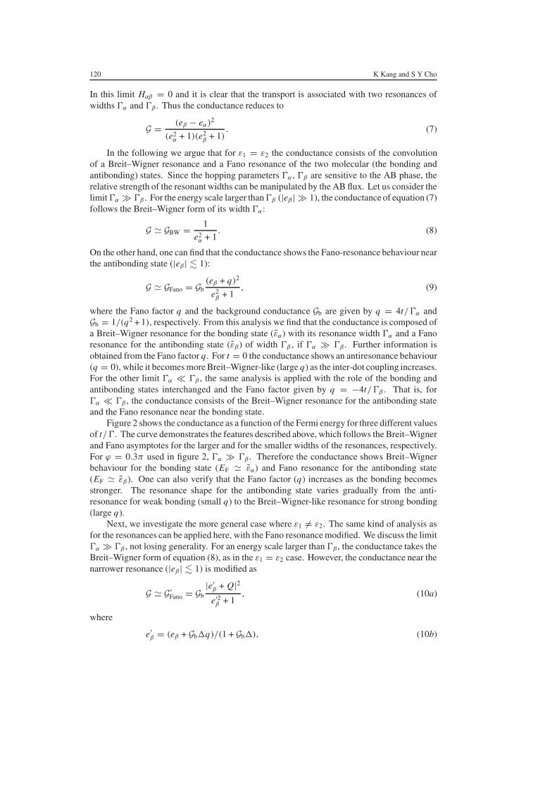
Figure 2 shows the conductance as a function of the Fermi energy for three different valuesof t/�. The curve demonstrates the features described above, which follows the Breit–Wignerand Fano asymptotes for the larger and for the smaller widths of the resonances, respectively.For ϕ = 0.3π used in figure 2, �α � �β . Therefore the conductance shows Breit–Wignerbehaviour for the bonding state (EF � εα) and Fano resonance for the antibonding state(EF � εβ). One can also verify that the Fano factor (q) increases as the bonding becomesstronger. The resonance shape for the antibonding state varies gradually from the anti-resonance for weak bonding (small q) to the Breit–Wigner-like resonance for strong bonding(large q).

Next, we investigate the more general case where ε1 �= ε2. The same kind of analysis asfor the resonances can be applied here, with the Fano resonance modified. We discuss the limit�α � �β , not losing generality. For an energy scale larger than �β , the conductance takes theBreit–Wigner form of equation (8), as in the ε1 = ε2 case. However, the conductance near thenarrower resonance (|eβ | � 1) is modified as

G � G′Fano = Gb

|e′β + Q|2e′2β + 1

, (10a)

where

e′β = (eβ + Gb�q)/(1 + Gb�), (10b)

Tunable molecular resonances of a double quantum dot Aharonov–Bohm interferometer 121

Figure 2. Dimensionless conductance (G) as a function of the Fermi energy (full curves) forthree different values of the inter-dot tunnelling (t/� = 0, 0.2, 1). Other parameters are givenby ε1 = ε2 = 0, ϕ = 0.3π . Long and short dashed curves denote the Breit–Wigner and Fanoasymptotes given in equations (8) and (9), respectively. The Fano factors for the Fano asymptotesare given by q = 0, 0.423 and 2.115 for t/� = 0, 0.2, 1, respectively.

and the modified Fano factor given by

Q = q1 − Gb�

1 + Gb�+ i

2√

�

1 + Gb�. (10c)

Equation (10a) can be regarded as a generalized Fano resonance formula with the complexFano factor Q. As pointed out in [23], the Fano factor is a complex number in the absenceof time reversal symmetry, for example by applying an external magnetic field. This pointwas addressed experimentally with an AB interferometer containing a single quantum dot [7].Note that the Fano factor in equation (10c) reduces to a real number in the absence of themagnetic field, because � → ∞ for ϕ = 0 as one can find from equation (6c).

Two significant changes are found in equation (10a) compared to equation (9).

(i) Since the modified Fano factor Q is a complex number in general, a transmission zerodoes not exist for ε1 �= ε2, unlike the covalent bonding limit.

(ii) The width of the Fano resonance becomes broader due to the difference in energy levelsbetween the dots:

�′β = �β + Gb

(�ε)2

�α

. (11)

For a fixed value of �ε, one can find that the broadening of the resonance is significant forsmall inter-dot coupling, recalling the relation Gb = 1/(q2 + 1) with q = 4t/�α .

The conductance as a function of Fermi energy for the case of different energy levels isshown in figure 3. Since �α � �β for ϕ = 0.3π , the conductance shows again the Breit–Wigner resonance behaviour for the larger energy scale corresponding to the ‘bonding’ state.The modified Fano resonance can be observed for the ‘antibonding’ state. The imaginary partof the modified Fano factor increases as the bonding strength becomes stronger, which impliesthat the shape of the resonance for the antibonding state varies gradually from the antiresonanceto the Breit–Wigner resonance. One can also verify that the width of the Fano resonance isbroader compared to the case of ε1 = ε2.

122 K Kang and S Y Cho

Figure 3. Dimensionless conductance (G) as a function of the Fermi energy (full curves) forthree different values of the inter-dot tunnelling (t/� = 0, 0.2, 1). Other parameters are givenby ε1 = −0.5�, ε2 = 0.5�, ϕ = 0.3π . Long and short dashed curves denote the Breit–Wignerand generalized Fano asymptote given by equations (8) and (10a), respectively. The generalizedFano factors for the asymptotes are given by Q = 0.753i, −0.258 + 0.861i, 0.128 + 2.335i fort/� = 0, 0.2, 1, respectively.

Finally, we discuss the Aharonov–Bohm oscillations of the conductance for the molecularstates and show that information about the bonding properties can be obtained by the oscillationpatterns. As shown in figure 4, the oscillation patterns of the ionic bonding limit are verydifferent from those of the covalent bonding limit. Above all, the periodicity is 2π in the ionicbonding limit while it becomes 4π in the covalent bonding limit. This periodicity variationcan be interpreted in terms of the effective coupling strength between the two dots. In the ionicbonding limit of |�ε| � 2t , the AB oscillation has the usual 2π periodicity since the couplingbetween the dots is ineffective. However, in the covalent bonding limit, the coupling betweendots becomes important and this strong effective coupling separates the interferometer into twosub-regions with their cross-sectional area halved. Therefore the oscillation period is doubled.

Comparing the AB oscillations of the bonding (figure 4(b)) and the antibonding(figure 4(c)) states, one finds that there are phase differences of 2π between the correspondingeigenstates. This originates from the difference of the wavefunction symmetry of the twoeigenstates.

It should be noted that our discussions on the AB oscillation characterizing the bondingproperties (ionic, covalent) can be applied only when the two regions divided by the directtunnelling have the same area. Though it seems possible to have devices with the same effectiveareas from the current nanofabrication technology, the two regions may have different areasin practice. In this case, the AB oscillations become more complicated and will show a kindof ‘quantum beating’ originating from the difference in area, which we do not address furtherhere.

In conclusion, we have investigated resonant tunnelling through the molecular states inan Aharonov–Bohm interferometer composed of two coupled quantum dots. We have foundthat the two resonances are composed of a Breit–Wigner resonance and a Fano resonance, forwhich the widths and the Fano factor depend on the AB phase. Further, we have suggestedthat the bonding properties and their symmetries can be characterized by the AB oscillation.

Tunable molecular resonances of a double quantum dot Aharonov–Bohm interferometer 123

Figure 4. (a) Molecular two-level energies as a function of the difference between the energylevels of the quantum dots. (b) AB oscillations for the bonding states with �ε/t = 0 (full curve),�ε/t = 1/3 (long dashed curve), �ε/t = 1 (short dashed curve) and �ε/t = 10/3 (dotted curve),marked in (a) as S0, S1, S2 and S3, respectively. (c) AB oscillations for the antibonding states with�ε/t = 0 (full curve), �ε/t = 1/3 (long dashed curve), �ε/t = 1 (short dashed curve) and�ε/t = 10/3 (dotted curve), marked in (a) as A0, A1, A2 and A3, respectively.

124 K Kang and S Y Cho

Acknowledgments

We wish to acknowledge H-W Lee for useful discussions and comments. This work has beensupported by the Korean Ministry of Information and Communication.

References

[1] Kastner M A 1993 Phys. Today 46 (1) 24[2] Kouwenhoven L P, Austing D G and Tarucha S 2001 Rep. Prog. Phys. 64 701[3] For a review see e.g. van der Wiel W G, De Franceschi S, Elzerman J M, Fujisawa T, Tarucha S and

Kouwenhoven L P 2003 Rev. Mod. Phys. 75 1[4] van der Vaart N C et al 1995 Phys. Rev. Lett. 74 4702[5] Yacoby A, Heiblum M, Mahalu D and Shtrikman H 1995 Phys. Rev. Lett. 74 4047[6] Schuster R, Buks E, Heiblum M, Mahadu D, Umansky V and Shtrikman H 1997 Nature 385 417[7] Kobayashi K, Aikawa H, Katsumoto S and Iye Y 2002 Phys. Rev. Lett. 88 256806[8] van der Wiel W G, De Franceschi S, Fujisawa T, Elzerman J M, Tarucha S and Kouwenhoven L P 2000 Science

289 2105[9] Ji Y, Heiblum M, Sprinzak D, Mahalu D and Shtrikman H 2000 Science 290 779

Ji Y, Heiblum M and Shtrikman H 2002 Phys. Rev. Lett. 88 076601[10] Gerland U, von Delft J, Costi T A and Oreg Y 2000 Phys. Rev. Lett. 84 3710[11] Kang K and Shin S-C 2000 Phys. Rev. Lett. 85 5619

Cho S Y, Kang K, Kim C K and Ryu C-M 2001 Phys. Rev. B 64 033314Kang K, Cho S Y and Park K W 2002 Phys. Rev. B 66 075312

[12] Bulka B R and Stefanski P 2001 Phys. Rev. Lett. 86 5128[13] Hofstetter W, Konig J and Schoeller H 2001 Phys. Rev. Lett. 87 156803[14] Kang K and Craco L 2002 Phys. Rev. B 65 033302[15] Holleitner A W, Decker C R, Qin H, Eberl K and Blick R H 2001 Phys. Rev. Lett. 87 256802

Holleitner A W, Blick R H, Huttel A K, Eberl K and Kotthaus J P 2002 Science 297 70[16] Kubala B and Konig J 2002 Phys. Rev. B 65 245301[17] Akera H 1993 Phys. Rev. B 47 6835[18] Izumida W, Sakai O and Shimizu Y 1997 J. Phys. Soc. Japan 66 717[19] Cho S Y, McKenzie R H, Kang K and Kim C K 2003 J. Phys.: Condens. Matter 15 1147[20] Loss D and Sukhorukov E V 2000 Phys. Rev. Lett. 84 1035[21] See, for example, Mahan G D 1990 Many-Particle Physics 2nd edn (New York: Plenum)[22] Meir Y and Wingreen N S 1992 Phys. Rev. Lett. 68 2512[23] Clerk A A, Waintal X and Brouwer P W 2001 Phys. Rev. Lett. 86 4636