trim, control, and performance effects in variable
TRANSCRIPT

TRIM, CONTROL, AND PERFORMANCE EFFECTS INVARIABLE-COMPLEXITY HIGH-SPEED CIVIL
TRANSPORT DESIGN
By
Peter Edward MacMillin
Thesis submitted to the faculty of the
virginia polytechnic institute and state university
in partial fulfillment of the requirements for the degree of
Masters of Science
in
Aerospace Engineering
William H. Mason, Chairman
Bernard Grossman Frederick H. Lutze
May 1996
Blacksburg, Virginia

TRIM, CONTROL, AND PERFORMANCE EFFECTS
IN VARIABLE-COMPLEXITY
HIGH-SPEED CIVIL TRANSPORT DESIGN
by
Peter Edward MacMillin
Committee Chairman: William H. Mason
Aerospace Engineering
(ABSTRACT)
Numerous trim, control requirements and mission generalizations have been made
to our previous multidisciplinary design methodology for a high speed civil trans-
port. We optimize the design for minimum take off gross weight, including both
aerodynamics and structures to find the wing planform and thickness distribution,
fuselage shape, engine placement and thrust, using 29 design variables. While adding
trim and control it was found necessary to simultaneously consider landing gear in-
tegration. We include the engine-out and crosswind landing requirements, as well
as engine nacelle ground strike for lateral-directional requirements. For longitudinal
requirements we include nose-wheel lift-off rotation and approach trim as the critical
conditions. We found that the engine-out condition and the engine nacelle ground
strike avoidance were critical conditions. The addition of a horizontal tail to provide
take-off rotation resulted in a significant weight penalty, and that penalty proved to
be sensitive to the position of the landing gear. We include engine sizing with thrust
during cruise and balanced field length conditions. Both the thrust during cruise
and balanced field length constraints were critical. We include a subsonic leg in our
mission analysis. The addition of a subsonic mission requirement also results in a
large weight penalty.
Acknowledgments
This work was supported by the NASA Langley Research Center under grant NAG1-
1160. Peter Coen is the grant monitor. We also wish to acknowledge the support of
Arnie McCullers of Vigyan and author of FLOPS for his considerable assistance.
This work would not have been possible without the previous work done by nu-
merous graduate students, notably Matthew Hutchison and Eric Unger. I would also
like to thank Hugh Weiss for keeping the computer systems running and keeping me
on the ball. A big thanks to everyone in the lab who made me laugh. Finally, a
special thanks to Bethany Falter for her innovative aircraft design ideas and Gina
Signori for her determined friendship.
iii

List of Symbols
ax horizontal acceleration
az vertical acceleration
A horizontal acceleration coefficient
AN engine nozzle area
AR aspect ratio, b2/S
ARv geometric aspect ratio for the isolated vertical tail
ARveff effective vertical tail aspect ratio
b wing span
bf rudder span
B horizontal acceleration coefficient
c mean aerodynamic chord
cg mean geometric chord
cg center of gravity
C horizontal acceleration coefficient
C1 constant used in calculating CDlg
CD drag coefficient, D/qS
CDi induced drag coefficient
CDlg landing gear drag coefficient
CDt coefficient of drag due to lift
CDwm windmilling engine drag coefficient
C` section lift coefficient
Cl rolling moment coefficient
Clβ dihedral effect stability derivative, ∂Cl/∂β
iv
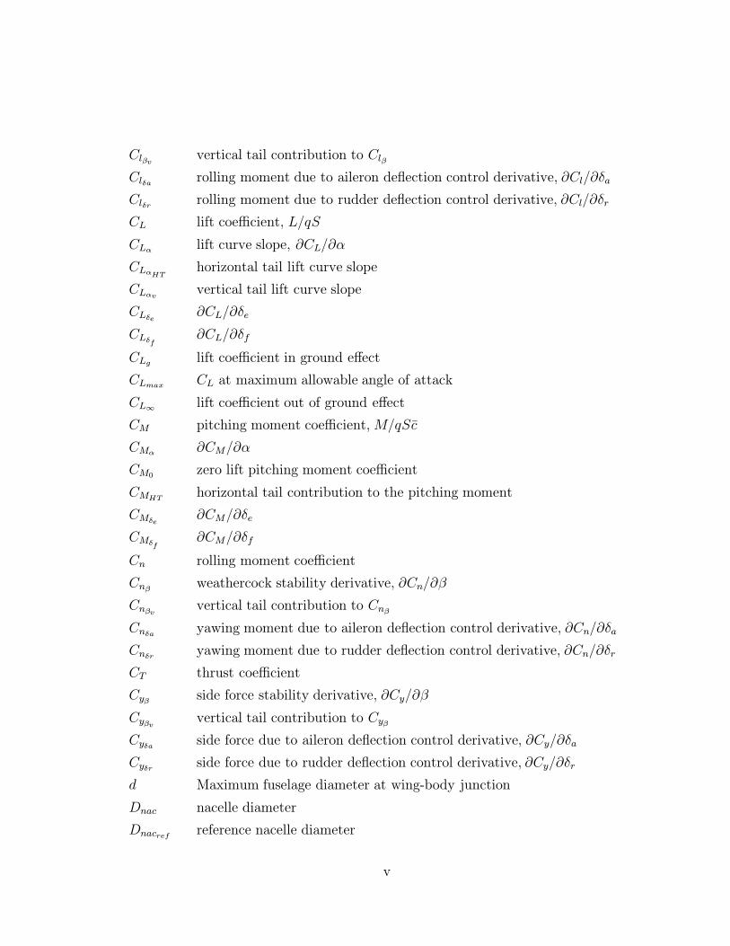
Clβv vertical tail contribution to Clβ
Clδa rolling moment due to aileron deflection control derivative, ∂Cl/∂δa
Clδr rolling moment due to rudder deflection control derivative, ∂Cl/∂δr
CL lift coefficient, L/qS
CLα lift curve slope, ∂CL/∂α
CLαHT horizontal tail lift curve slope
CLαv vertical tail lift curve slope
CLδe ∂CL/∂δe
CLδf ∂CL/∂δf
CLg lift coefficient in ground effect
CLmax CL at maximum allowable angle of attack
CL∞ lift coefficient out of ground effect
CM pitching moment coefficient, M/qSc
CMα ∂CM/∂α
CM0 zero lift pitching moment coefficient
CMHThorizontal tail contribution to the pitching moment
CMδe∂CM/∂δe
CMδf∂CM/∂δf
Cn rolling moment coefficient
Cnβ weathercock stability derivative, ∂Cn/∂β
Cnβv vertical tail contribution to Cnβ
Cnδa yawing moment due to aileron deflection control derivative, ∂Cn/∂δa
Cnδr yawing moment due to rudder deflection control derivative, ∂Cn/∂δr
CT thrust coefficient
Cyβ side force stability derivative, ∂Cy/∂β
Cyβv vertical tail contribution to Cyβ
Cyδa side force due to aileron deflection control derivative, ∂Cy/∂δa
Cyδr side force due to rudder deflection control derivative, ∂Cy/∂δr
d Maximum fuselage diameter at wing-body junction
Dnac nacelle diameter
Dnacref reference nacelle diameter
v

f(x) analysis function
fd(x) detailed model analysis function
fs(x) simple model analysis function
Fmg main landing gear reaction force
g gravitational acceleration
h height above ground
he energy height
it horizontal tail deflection
I airfoil leading edge radius parameter
Iyymg Moment of inertia about the main gear
k empirical factor used to calculate Cyβv , see Fig. 8
kr factor used to calculate the rotation speed
K ′ rudder effectiveness parameter
Kb parameter used to calculate Cyδr , defined by Eq. 13
`mg length of the main gear
`v horizontal distance between aircraft cg and vertical tail aerodynamic
center, see Fig. 9
lnac nacelle length
lnacref reference nacelle length
Lext net rolling moment
m chordwise location of maximum airfoil thickness
m engine mass flow
mref reference engine mass flow
Mcg pitching moment about the center of gravity
Mmg pitching moment about the main gear
Next net yawing moment
Ps specific excess power
q dynamic pressure, 12ρV 2
ri engine inlet radius
rt leading edge radius to chord ratio
R horizontal acceleration solution parameter, B2 − 4AC
vi

seng constant used to calculate engine weight
S wing area
SHT horizontal tail wing area
Sv vertical tail area
t time
t/c airfoil thickness to chord ratio
T thrust
T0, T1, T2 thrust coefficients
Tref reference thrust
V Aircraft velocity
Vcrit critical engine failure speed
Vcritg guess for Vcrit
VH horizontal tail volume coefficient
VMC minimum control speed
VN engine nozzle velocity
Vr rotation speed
Vs stall speed
Vx horizontal component of the aircraft velocity
Vz vertical component of the aircraft velocity
W aircraft weight
Weng engine weight
Wengref reference engine weight
x vector of design variables
x0 vector of initial design variables
xBFL balanced field length distance
xcg horizontal distance from nose of aircraft to cg
xcgmg horizontal distance between the cg and the main gear contact point
xLcg horizontal distance between the aerodynamic center and the cg
xLmg horizontal distance between the aerodynamic center and the main gear
contact point
xmain horizontal distance from nose of aircraft to main landing gear
vii

xnose horizontal distance from nose of aircraft to nose gear
xTmg horizontal distance between the thrust vector and the main gear contact
point
X horizontal distance
Yext net side force
zcgmg vertical distance between the cg and the main gear contact point
zDcg vertical distance between the aerodynamic center and the cg
zDmg vertical distance between the aerodynamic center and the main gear
contact point
zTcg vertical distance between the thrust vector and the cg
zTmg vertical distance between the thrust vector and the main gear contact
point
Zv vertical distance between aircraft cg and vertical tail aerodynamic
center, see Fig. 9
Zw vertical distance from the wing root quarter chord point to
the fuselage centerline, positive downward
Greek Symbols
α angle of attack[(αδ)CL(αδ)C`
]Defined in Figure 10
(αδ)C` Defined in Figure 10
β sideslip angle
βg parameter for calculating CLg
βM√
1−M2
δa aileron deflection, positive down
δe elevator deflection, positive down
δf flap deflection, positive down
δr rudder deflection, positive to the left (results in positive side force)
ηv dynamic pressure ratio for vertical tail
γ flight path angle
viii

Λc/2half chord sweep angle
Λc/4quarter chord sweep angle
ΛT thrust vectoring angle
µgrd coefficient of friction of the runway
φ bank angle
ρ atmospheric density
ρ0 atmospheric density at sea level
σ atmospheric density ratio, ρ/ρ0
σg parameter for calculating ground effects
σ(x) scaling functiondσdβ
sidewash factor
τTE airfoil trailing edge half angle
θmg pitch rate about the main gear
ε downwash angle
Subscripts
a initial point
b final point
Superscripts
˙ first derivative with respect to time
¨ second derivative with respect to time
Acronyms
BFL Balanced Field Length
FLOPS FLight OPtimization System
HSCT High-Speed Civil Transport
MDO Multidisciplinary Design Optimization
TOGW Take Off Gross Weight
VCM Variable-Complexity Modeling
VLM Vortex Lattice Method
ix

x

Contents
Abstract ii
Acknowledgments iii
List of Symbols iv
1 Introduction 1
2 Design Issues 6
2.1 Vertical Tail Sizing . . . . . . . . . . . . . . . . . . . . . . . . . . . . 7
2.2 Engine Location Limits . . . . . . . . . . . . . . . . . . . . . . . . . . 8
2.3 Nacelle and Wing Tip Strike . . . . . . . . . . . . . . . . . . . . . . . 8
2.4 Landing Gear Location . . . . . . . . . . . . . . . . . . . . . . . . . . 10
2.5 Horizontal Tail Sizing . . . . . . . . . . . . . . . . . . . . . . . . . . . 12
2.6 Engine Sizing . . . . . . . . . . . . . . . . . . . . . . . . . . . . . . . 12
3 Design Formulation 13
3.1 Design Variables . . . . . . . . . . . . . . . . . . . . . . . . . . . . . 13
3.2 Constraints . . . . . . . . . . . . . . . . . . . . . . . . . . . . . . . . 18
4 Variable Complexity Modeling 21
5 Analysis Methods 24
5.1 Aerodynamics . . . . . . . . . . . . . . . . . . . . . . . . . . . . . . . 24
5.2 Structures . . . . . . . . . . . . . . . . . . . . . . . . . . . . . . . . . 27
xi
5.3 Center of Gravity and Inertia Estimation . . . . . . . . . . . . . . . . 28
5.4 Stability Derivative Estimation . . . . . . . . . . . . . . . . . . . . . 29
5.4.1 Lateral-Directional Derivatives . . . . . . . . . . . . . . . . . . 29
5.4.2 Accuracy of Lateral-Directional Estimates . . . . . . . . . . . 32
5.4.3 Longitudinal Derivatives . . . . . . . . . . . . . . . . . . . . . 33
5.5 Landing Gear . . . . . . . . . . . . . . . . . . . . . . . . . . . . . . . 35
5.6 Engine Out . . . . . . . . . . . . . . . . . . . . . . . . . . . . . . . . 35
5.7 Crosswind Landing . . . . . . . . . . . . . . . . . . . . . . . . . . . . 36
5.8 Take Off Analysis . . . . . . . . . . . . . . . . . . . . . . . . . . . . . 36
5.9 Takeoff Aerodynamics . . . . . . . . . . . . . . . . . . . . . . . . . . 41
5.10 Powered Approach Trim . . . . . . . . . . . . . . . . . . . . . . . . . 43
5.11 Engine Scaling . . . . . . . . . . . . . . . . . . . . . . . . . . . . . . 44
5.12 Minimum Time Climb with Dynamic Pressure Constraint . . . . . . . 44
5.13 Optimization Strategies . . . . . . . . . . . . . . . . . . . . . . . . . 46
6 Results 47
6.1 Baseline Optimization (Case 26a) . . . . . . . . . . . . . . . . . . . . 48
6.2 Vertical Tail Considerations . . . . . . . . . . . . . . . . . . . . . . . 48
6.2.1 Case 27a . . . . . . . . . . . . . . . . . . . . . . . . . . . . . . 52
6.2.2 Case 27b . . . . . . . . . . . . . . . . . . . . . . . . . . . . . . 54
6.3 Vertical and Horizontal Tail Considerations . . . . . . . . . . . . . . . 61
6.3.1 Case 28a . . . . . . . . . . . . . . . . . . . . . . . . . . . . . . 61
6.3.2 Case 28b . . . . . . . . . . . . . . . . . . . . . . . . . . . . . . 61
6.4 Engine Sizing (Case 29a) . . . . . . . . . . . . . . . . . . . . . . . . . 66
6.5 Subsonic Leg (Case 29b) . . . . . . . . . . . . . . . . . . . . . . . . . 67
6.6 Minimum Time to Climb Calculation . . . . . . . . . . . . . . . . . . 72
7 Conclusions 73
References 76
xii

A Using the HSCT code 83
A.1 Input files . . . . . . . . . . . . . . . . . . . . . . . . . . . . . . . . . 83
A.2 Output files . . . . . . . . . . . . . . . . . . . . . . . . . . . . . . . . 84
A.3 Other files . . . . . . . . . . . . . . . . . . . . . . . . . . . . . . . . . 85
A.4 The hsct.command file . . . . . . . . . . . . . . . . . . . . . . . . . . 86
A.4.1 Parameter sections . . . . . . . . . . . . . . . . . . . . . . . . 86
A.4.2 Commands . . . . . . . . . . . . . . . . . . . . . . . . . . . . 90
A.5 Experiences optimizing with the HSCT code . . . . . . . . . . . . . . 92
A.6 Sample hsct.command file . . . . . . . . . . . . . . . . . . . . . . . . 93
A.7 Sample design variable file . . . . . . . . . . . . . . . . . . . . . . . . 95
B HSCT Code Structure 96
B.1 Overview of code structure . . . . . . . . . . . . . . . . . . . . . . . . 96
B.2 aero.c . . . . . . . . . . . . . . . . . . . . . . . . . . . . . . . . . . . 98
B.3 craidio.c . . . . . . . . . . . . . . . . . . . . . . . . . . . . . . . . . 100
B.4 dataio.c . . . . . . . . . . . . . . . . . . . . . . . . . . . . . . . . . 102
B.5 f77iface.c . . . . . . . . . . . . . . . . . . . . . . . . . . . . . . . . 103
B.6 fminbr.c . . . . . . . . . . . . . . . . . . . . . . . . . . . . . . . . . 104
B.7 main.c . . . . . . . . . . . . . . . . . . . . . . . . . . . . . . . . . . . 105
B.8 modify.c . . . . . . . . . . . . . . . . . . . . . . . . . . . . . . . . . 105
B.9 numerics.c . . . . . . . . . . . . . . . . . . . . . . . . . . . . . . . . 107
B.10 options.c . . . . . . . . . . . . . . . . . . . . . . . . . . . . . . . . . 109
B.11 perform.c . . . . . . . . . . . . . . . . . . . . . . . . . . . . . . . . . 110
B.12 servmath.c . . . . . . . . . . . . . . . . . . . . . . . . . . . . . . . . 112
B.13 simpaero.c . . . . . . . . . . . . . . . . . . . . . . . . . . . . . . . . 112
B.14 stability.c . . . . . . . . . . . . . . . . . . . . . . . . . . . . . . . 116
B.15 takeoff.c . . . . . . . . . . . . . . . . . . . . . . . . . . . . . . . . . 118
B.16 util.c . . . . . . . . . . . . . . . . . . . . . . . . . . . . . . . . . . . 121
B.17 weight.c . . . . . . . . . . . . . . . . . . . . . . . . . . . . . . . . . 124
B.18 flops inter.f . . . . . . . . . . . . . . . . . . . . . . . . . . . . . . 125
B.19 harris.f . . . . . . . . . . . . . . . . . . . . . . . . . . . . . . . . . 126
xiii

B.20 optimizer.f . . . . . . . . . . . . . . . . . . . . . . . . . . . . . . . 130
B.21 rs weight.f . . . . . . . . . . . . . . . . . . . . . . . . . . . . . . . . 130
B.22 sfeng.f . . . . . . . . . . . . . . . . . . . . . . . . . . . . . . . . . . 131
B.23 sfwate.f . . . . . . . . . . . . . . . . . . . . . . . . . . . . . . . . . 131
VITA 132
xiv

List of Tables
1 Design Variables . . . . . . . . . . . . . . . . . . . . . . . . . . . . . 15
2 Optimization Constraints . . . . . . . . . . . . . . . . . . . . . . . . . 19
3 Load cases used in structural optimization . . . . . . . . . . . . . . . 28
4 Comparison of stability and control derivative estimations for the XB-
70A . . . . . . . . . . . . . . . . . . . . . . . . . . . . . . . . . . . . 33
5 Comparison of stability and control derivative estimations for a F/A-18
at Mach 0.2, out of ground effect . . . . . . . . . . . . . . . . . . . . 34
6 Overview of results . . . . . . . . . . . . . . . . . . . . . . . . . . . . 47
7 Comparison of Initial and Final Designs, Case 26a . . . . . . . . . . . 50
8 Comparison of Initial and Final Designs, Case 27a . . . . . . . . . . . 54
9 Comparison of Initial and Final Designs, Case 27b . . . . . . . . . . . 58
10 Comparison of Initial and Final Designs, Case 28a . . . . . . . . . . . 62
11 Comparison of Initial and Final Designs, Case 28b . . . . . . . . . . . 65
12 Comparison of Initial and Final Designs, Case 29a . . . . . . . . . . . 68
13 Comparison of Initial and Final Designs, Case 29b . . . . . . . . . . . 71
14 Summary of optimizations . . . . . . . . . . . . . . . . . . . . . . . . 73
xv

List of Figures
1 Wing and vertical tail weights versus spanwise nacelle location . . . . 9
2 Wave drag versus vertical tail size . . . . . . . . . . . . . . . . . . . . 9
3 Definition of tipback angle . . . . . . . . . . . . . . . . . . . . . . . . 11
4 Definition of the overturn angle . . . . . . . . . . . . . . . . . . . . . 11
5 Planform Definition Parameters . . . . . . . . . . . . . . . . . . . . . 16
6 Airfoil Thickness Parameters . . . . . . . . . . . . . . . . . . . . . . . 17
7 Effect of increasing semi-span on wave drag prediction . . . . . . . . 26
8 Definition of k for Cyβv . . . . . . . . . . . . . . . . . . . . . . . . . . 30
9 Definition of `v and Zv . . . . . . . . . . . . . . . . . . . . . . . . . . 31
10 Definition of[
(αδ)CL(αδ)C`
]. . . . . . . . . . . . . . . . . . . . . . . . . . . 32
11 Specific excess power contours for a HSCT configuration . . . . . . . 45
12 Convergence of Case 26a . . . . . . . . . . . . . . . . . . . . . . . . . 49
13 Initial and final planforms, Case 26a . . . . . . . . . . . . . . . . . . 49
14 History of wing weight and trailing edge sweep, Case 26a . . . . . . . 50
15 History of drag due to lift, at CL = 0.1, Case 26a . . . . . . . . . . . 51
16 History of wave drag, Case 26a . . . . . . . . . . . . . . . . . . . . . 51
17 History of total drag, at CL = 0.1, Case 26a . . . . . . . . . . . . . . 52
18 Convergence of Case 27a . . . . . . . . . . . . . . . . . . . . . . . . . 53
19 Initial and final planforms, Case 27a . . . . . . . . . . . . . . . . . . 53
20 History of nacelle positions and vertical tail area . . . . . . . . . . . . 55
21 History of Cyβ , Clβ , and Cnβ for Case 27a . . . . . . . . . . . . . . . . 56
22 History of Cyδr , Clδr , and Cnδr for Case 27a . . . . . . . . . . . . . . . 57
23 Initial and final planforms, Case 27b . . . . . . . . . . . . . . . . . . 58
xvi
24 History of Cyβ , Clβ , and Cnβ for Case 27b . . . . . . . . . . . . . . . . 59
25 History of Cyδr , Clδr , and Cnδr for Case 27b . . . . . . . . . . . . . . . 60
26 Initial and final planforms, Case 28a . . . . . . . . . . . . . . . . . . 62
27 Takeoff Gross Weight and Range convergence, Case 28a . . . . . . . . 63
28 Vertical Tail Size and Nacelle Location convergence, Case 28a . . . . 63
29 Horizontal Tail Size convergence, Case 28a . . . . . . . . . . . . . . . 64
30 Initial and final planforms, Case 28b . . . . . . . . . . . . . . . . . . 65
31 Initial and final planforms, Case 29a . . . . . . . . . . . . . . . . . . 67
32 Takeoff Gross Weight and Range convergence, Case 29a . . . . . . . . 68
33 Balanced field length convergence, case 29a . . . . . . . . . . . . . . . 69
34 Initial and final planforms, Case 29b . . . . . . . . . . . . . . . . . . 70
35 Takeoff Gross Weight convergence, Case 29b . . . . . . . . . . . . . . 70
36 Range and BFL convergence, case 29b . . . . . . . . . . . . . . . . . 71
xvii

Chapter 1
Introduction
Designing a supersonic transport is an extremely demanding task. Many of the mis-
sion requirements conflict with one another. To satisfy all of the requirements, the
designer must completely integrate the various technologies in the design, such as
trading supersonic cruising efficiency for takeoff and landing performance. The effi-
ciency and economic feasibility of the final design is determined by the quality of the
technology integration. To make intelligent compromises the designer requires data
from many disciplines and must be aware of the disciplinary interactions. If any of
the major disciplinary interactions are neglected in the conceptual/preliminary design
phase, it is likely there will be a significant weight penalty in the final design because
of the need to account for the neglected interactions after the configuration has been
frozen.
Multidisciplinary design optimization (MDO) is a methodology for the design of
systems where interactions between disciplines are explicitly addressed. For vehicles
designed for extremely demanding missions, MDO is an enabling technology, without
which the design goals will not be achieved. Sobieski has provided much of the
impetus for this approach and has written the key reviews describing MDO1, 2, 3. The
coupling inherent in MDO produces increased complexity, due in part to the increased
size of the MDO problem compared to single disciplinary optimization. The number
of design variables increases with each additional discipline. Since solution times
for most analysis and optimization algorithms increase at a superlinear rate, the
1

computational cost of MDO is usually much higher than the sum of the costs of the
single-discipline optimizations for the disciplines represented in the MDO. In this
work we focus on one area where this computational problem is acute: combined
aerodynamic-structural-controls-propulsion design of the high-speed civil transport
(HSCT).
Aircraft design at the conceptual level has always been multidisciplinary, because
the tradeoffs between the requirements of the different disciplines are easily addressed
due to the simplicity of the modeling of the system. Often these are statistically-
derived, experience-based algebraic models. At the preliminary design level, however,
more detailed numerical models of both structures and aerodynamics are employed.
Early studies of combined aerodynamic and structural optimization relied on sim-
ple aerodynamic and structural models and a small number of design variables4, so
that computational cost was not an issue. Rather, the goal was to demonstrate the
advantages of the optimized design. For example, Grossman et al.5 used lifting line
aerodynamics and beam structural models to demonstrate that simultaneous aerody-
namic and structural optimization can produce superior designs compared to the use
of a sequential approach. Similar models were used by Wakayama and Kroo6 who
showed that optimal designs are strongly affected by compressibility drag, aeroelas-
ticity and multiple structural-design conditions. Gallman et al.7 used beam structural
models together with vortex-lattice aerodynamics to explore the advantages of joined-
wing aircraft.
However, as soon as more detailed numerical simulations are considered it becomes
difficult to preserve interdisciplinary communications, and until recently, MDO has
not been used at the detailed design level. Modern single-disciplinary designs in
both aerodynamics and structures go well beyond simple models. Aerodynamic op-
timization for transports is often performed with three-dimensional nonlinear models
e.g., Euler equations 8. Structural optimization is performed with large finite-element
models. For example, Tzong9 performed a structural optimization with static aero-
elastic effects of a high-speed civil transport using a finite element model with 13,700
degrees of freedom and 122 design variables.
2

There is a corresponding pressure to use more detailed models in MDO. For ex-
ample, Borland10 performed a combined aerodynamic-structural optimization of a
subsonic transport wing with a fixed planform using a large finite-element model and
thin-layer Navier-Stokes aerodynamics. However, due to computational cost, they
only used three aerodynamic design variables along with 20 structural design vari-
ables.
The aerodynamic design and structural design of a wing are closely related, and
the tradeoff between structural weight and aerodynamic performance determines the
shape parameters of the wing, including thickness and aspect ratio. However, there
is a fundamental asymmetry in the level of detail that each discipline needs to sup-
ply the other. The structural designer needs detailed load distributions from the
aerodynamicist. Therefore, it is not possible to perform accurate structural opti-
mization with conceptual-level aerodynamics. In contrast, the aerodynamic designer
can perform aerodynamic optimization using only the structural weight. Of course,
accurate estimation of the sensitivities of the weight is also required for aerodynamic
optimization.
The structural weight, being an integral measure of the structure, is amenable to
accurate estimation by conceptual-level weight equations. Weight equations have tra-
ditionally been developed semi-analytically using actual wing weights. McCullers11
developed a transport weight function based on both historical data and structural
optimization solutions for numerous planform and thickness combinations. These
equations are used in the Flight Optimization System (FLOPS)11. Scott12, Udin
and Anderson13, and Torenbeek14 have discussed the considerations used in develop-
ing modern wing weight equations. Huang et al.15 compared the FLOPS equation
with both structural optimization and another wing weight equation for HSCT-class
planforms.
The high cost of using detailed analysis methods in an MDO procedure prevents
their use in conceptual design. To reduce the computational cost of MDO, we have
been developing the variable-complexity modeling concept. Variable-complexity mod-
eling uses multiple levels of analysis methods. The detailed numerical analysis meth-
ods are only used sparingly to improve the accuracy of the approximate analysis
3

methods. An in-depth discussion of the various types of variable-complexity approx-
imations and the aerodynamic and structural analysis methods we are using can be
found in the papers by Hutchison et al.16, 17, 18 and Dudley et al.19.
In this work we extend the previous work of Hutchison et al.16, 17, 18 to handle
additional mission details and to include trim, control and propulsion considerations
directly in the variable-complexity design procedure.
Explicit consideration of trim and control in conceptual aircraft sizing method-
ology is unusual. For subsonic configuration optimizations there have been related
studies by Sliwa20, 21 and by Gallman et al.7. Both considered longitudinal trim and
control, and both found that including trim and control considerations affected the
design. In the study by Gallman et al.7 the take-off rotation control requirement
was found to be a critical issue in the comparison of equivalent conventional and
joined-wing configurations.
We include vertical and horizontal tail sizing by examining critical stability and
control requirements, such as takeoff rotation and the engine out condition. As part
of the integration of aircraft trim and control requirements, the engine and landing
gear locations emerge as significant considerations. Both of these considerations are
included in the methodology described in this paper.
Stability derivatives must be available to include trim and control in the optimiza-
tion. We use our variable-complexity modeling concept to estimate them. Specifically,
we use the so-called interlacing technique described by Dudley et al.19. They used the
approach to incorporate detailed finite element structural analysis in the optimization.
We extend our mission requirements with the addition of a subsonic leg and a
minimum time climb with a dynamic pressure constraint. Most routes that this air-
craft might fly will require an initial subsonic leg to avoid sonic booms near populated
areas. We examine the effect of this on our design by requiring an initial portion of
our specified range be flown at Mach 0.9. The subsonic leg is flown at a much lower
altitude than the supersonic portion. We investigate using a minimum time to climb
profile to transition from the subsonic to the supersonic legs.
We include engine sizing using thrust scaling. Thrust required is determined by
examining mission thrust requirements and balanced field length (BFL). An HSCT
4

must be able to use existing runways, which limits the allowable BFL. One of the
most important factors in determining the BFL is the thrust to weight ratio of the
aircraft.
In the next chapter we discuss the design issues addressed in this work. Chapter
3 describes how we formulate our design problem. Variable-complexity modeling is
explained in detail in Chapter 4. Our analysis methods are described in Chapter 5.
In Ch. 6 we present our results and finally we discuss our conclusions in Chapter 7.
5

Chapter 2
Design Issues
The size, shape, and location of almost every component on an aircraft is determined
by various critical requirements. Often there are multiple issues affecting the design
of a component. Our work uses the conceptual/preliminary design control authority
assessment methods developed by Kay et al.22. In particular, Kay established a set
of stability and control requirements which must be addressed in the initial stages
of vehicle design. A study of control requirements specific to HSCT configurations
has recently been conducted by McCarty et al.23. Their work is consistent with the
approach of Kay, and has been used to focus the work presented here. The ratio of
dynamic pressure at cruise (M2.4 at 65K ft) to the low speed critical field performance
conditions (150kt, sea level) is more than 6. Thus, References [22] and [23] find that
the large control power requirements during take-off and landing combined with the
low dynamic pressure results in the low speed field performance conditions being the
critical design conditions.
Assuming the low speed conditions define the control surface sizes, we incorporate
trim and control requirements for both lateral-directional and longitudinal control
conditions. In the lateral-directional case, the conditions are engine-out trim per-
formance and crosswind landing. For engine-out trim performance we require the
aircraft be capable of trimmed flight after two engines on the same side fail. Thus
the vertical tail must be capable of handling the yawing moment generated by the
thrust imbalance. This is especially important since the wing weight decreases when
6

the engines are placed well outboard. This effect is exploited during the optimization,
sending the engines as far outboard as practical. In the longitudinal axis, take-off
rotation has been found to be the critical condition for this class of aircraft, and we
consider take-off rotation and approach trim. The engine location becomes impor-
tant because of both asymmetric thrust considerations and the requirement that the
engine nacelles not strike the runway during take-off and landing. The landing gear
location and length play a key role in defining the control power required to rotate
the aircraft at take-off. In the following sections we discuss what we consider to be
the critical issues for the vertical and horizontal tails, engines, and landing gear.
2.1 Vertical Tail Sizing
For civilian aircraft with four engines, where maneuverability is not a primary con-
sideration, the vertical tail size is based either on the requirement that the aircraft be
capable of trimmed flight with two engines inoperative as specified in FAR 25.147, or
to handle the crosswind landing requirement. The pilot must have sufficient control
authority to trim the aircraft in these situations, as well as to be able to perform nec-
essary maneuvers. Therefore, we require the aircraft be trimmed directionally using
no more than 75% of the maximum available control authority.
The engine out condition generates a yawing moment what must be balanced.
The magnitude of the yawing moment depends on the thrust of the engines, and
their positions. The crosswind landing condition requires the aircraft balance the
yawing moment caused by a 20 knot crosswind, as specified in FAR 25.237. Deflecting
the rudder creates the balancing yawing moment, but also causes a sideforce which
must be counteracted. This is done with a combination of sideslip and bank. Both
sideslip and bank can make landing difficult if the angle is too great. Large sideslip
causes rough landings as the aircraft must suddenly straighten out upon touchdown.
Excessive bank introduces the possibility of the wing tip scraping the ground before
the landing gear touches down. These considerations require us to limit the allowable
amount of sideslip and bank to 10◦ and 5◦, respectively. The rudder deflection also
creates a rolling moment that is usually controlled using the ailerons.
7

2.2 Engine Location Limits
Moving the engine outboard provides wing bending moment relief, thereby reducing
the wing weight. As the engine moves outboard, the vertical tail must increase in size
to satisfy the engine out condition. But, the increase in vertical tail weight is small
compared to the reduction in wing weight, as shown in Fig. 1. There is a practical
limit to the amount of wing bending moment relief moving the engine outboard can
produce. After this limit is reached, moving the engine further outboard does not
result in any further reduction in wing weight. But vertical tail size and weight
continue to increase. This produces a minimum in the sum of the wing and vertical
tail weights at the point where the limit is reached.
Also, the increase in drag due to increasing the vertical tail size and including
the associated movement of the nacelle is small, as shown in Fig. 2. The increase
in volumetric wave drag is less than two counts, and the increase in friction drag
is about three counts. Thus the minimum TOGW is achieved using a very large
vertical tail and placing the engine at the point where the limit in wing bending
moment is achieved. Placing the engine extremely far outboard could cause problems
with flutter, engine-out trim, nacelle strike during landing, and airframe stresses
during ground operations, such as full fuel taxi. A constraint is needed to prevent
the optimizer from placing the engines too far outboard on the wing.
2.3 Nacelle and Wing Tip Strike
HSCT configurations generally have low lift curve slopes. This results in high landing
angles of attack, approximately 12◦. When landing at such a high angle of attack,
it is possible for the engine nacelles to strike the runway. This is dependent on the
positioning of the nacelles, with 25% overhang, and the sweep of the wing trailing
edge, as well as the length and position of the landing gear. An allowance must also
be made for up to 5◦ of bank.
A similar problem exists with the wing tips. A large amount of trailing edge sweep
can place the trailing edge of the wing tip well behind the main gear. When this is
8

74000
76000
78000
80000
82000
84000
86000
88000
1500
2000
2500
3000
3500
4000
4500
5000
0 10 20 30 40 50 60 70
Win
g w
eigh
t (l
bs)
Vertical T
ail weight (lbs)
Spanwise nacelle location (ft)
Wing weight
Vertical Tail weight
Wing + Tail weight
Figure 1: The sum of the wing and vertical tail weights decreases as the engine ismoved outboard.
0.0012
0.0013
0.0014
0.0015
0.0016
0.0017
0.0037
0.0038
0.0039
0.0040
0.0041
0.0042
200 400 600 800 1000 1200 1400 1600
Wav
e dr
ag
Friction drag
Vertical Tail area (ft2)
Wave drag
Friction drag
Figure 2: The wave drag increases very little with nacelles moving outboard andincreasing vertical tail area.
9

coupled with the relatively high landing angle of attack and even a small amount of
bank, it can cause the wing tips to strike the runway.
2.4 Landing Gear Location
Landing gear position relative to the center of gravity is important for take-off ro-
tation, as well as the effect on the engine nacelle strike constraint. Both the nose
and main gear positions must be known for the center of gravity calculation. On
landing, the main gear touches down first, so the position and length of the main
gear is critical to the nacelle and wing tip strike constraints. Increasing the length
of the main gear results in more ground clearance, which is the distance between the
nacelles and the runway. Moving the main landing gear closer to the engines on the
wing reduces the effect of pitch and bank on the ground clearance. In general, pitch
will reduce nacelle ground clearance and banking will further reduce ground clearance
on the wing which is banked toward the ground.
The weight distribution on the landing gear is important during take-off rotation.
If the nose gear is too heavily loaded, it will be difficult to rotate to the take-off
attitude. If the nose gear is too lightly loaded, the aircraft will be hard to steer
and could rotate before there is enough control authority to control the aircraft’s
attitude. Torenbeek24 recommends the nose gear support between 8% and 15% of the
total weight. We elected to place the nose gear so that it would be supporting 11.5%
of the total weight.
Other important considerations include the tipback and overturn angles. Both
angles relate the main gear’s position to the location of the center of gravity. The
tipback angle is the angle between the main gear and the cg as seen in the side view,
as seen in Fig. 3, and it should be 15◦ or less. If the main gear is not far enough
behind the center of gravity, the aircraft could tip back on its tail. As the tipback
angle is increased, the pitching moment required to rotate the aircraft for takeoff also
increases. The horizontal tail size is very sensitive to this parameter. The overturn
angle is a measure of the likelihood of the aircraft tipping over sideways while taxiing
in a turn. It should be less than 63◦, as shown in Figure 4.
10

Static Ground Line
SIDE VIEW
15˚ Tipback angle
Main gear
Figure 3: Definition of tipback angle
A
A
View A-A
Stat
icG
roun
d L
ine
PLAN VIEW Overturnangle
Figure 4: Definition of the overturn angle
11
2.5 Horizontal Tail Sizing
Several longitudinal control and trim issues are important. The field performance re-
quirements are among the most critical. For most airplanes, take-off involves rotating
on the main landing gear to a pitch attitude at which the wings can generate enough
lift to become airborne. This rotation is caused by the pitching moment generated
by a longitudinal control effector, such as the horizontal tail or the wing trailing edge
flap for a tailless configuration. The civilian FAR25 regulations require the aircraft be
able to take off safely. If the takeoff rotation requires too much time, it will greatly
increase the takeoff distance. This limits the number of airports that the aircraft can
use. We require the aircraft be able to rotate to lift-off in under 5 sec∗.
Approach trim is also important. The aircraft must be able to be trimmed at an
angle of attack well above normal operating conditions. There should also be enough
additional control power beyond trim to maneuver. This allows the pilot to deal
with gusts and emergencies. For unstable aircraft, the actual amount of nose down
pitching moment at high angle of attack required for safe flight is a current research
topic26.
2.6 Engine Sizing
Engine size is determined primarily by bypass ratio and the maximum massflow the
engine is required to handle. The maximum massflow is proportional to the maximum
thrust the engine can produce. So, for a given bypass ratio, the size of the engine is
based on the maximum thrust required.
Lower thrust requirements mean a lighter, smaller engine, which creates less drag,
can be used. But less thrust also means longer takeoff lengths. The second segment
climb requirements are sometimes the critical conditions for sizing the engine. Also,
the thrust available during flight must be sufficient to overcome drag. It is desirable
to use the smallest engine possible, while satisfying all of the mission requirements.
∗This requirement was determined by investigating typical rotation times for large aircraft. Sincethere are very few aircraft of this type there is not a large body of data to base our requirement on.Requiring the aircraft to rotate in under 5 sec is a somewhat arbitrary but reasonable assumption.
12

Chapter 3
Design Formulation
Our design problem is to optimize an HSCT configuration to minimize takeoff gross
weight (TOGW) for a range of 5500 n.mi., and 251 passengers. Our main mission is
a supersonic cruise-climb at Mach 2.4 with a maximum altitude of 70,000 ft. In this
work, we expand our mission to include take off, a subsonic cruise at Mach 0.9, and
a minimum time climb with a dynamic pressure limit.
The choice of gross weight as the figure of merit (objective function) directly in-
corporates both aerodynamic and structural considerations, in that the structural de-
sign directly affects aircraft empty weight and drag, while aerodynamic performance
dictates the required fuel weight. Trim, control, and propulsion requirements are
explicitly treated also. The current work incorporates the influence of structural con-
siderations in the aerodynamic design by a variable-complexity modeling approach.
We employ the weight equations of McCullers11. A procedure called interlacing is
used to estimate stability and control derivatives. Variable-complexity modeling and
interlacing will be described in Chapter 4.
3.1 Design Variables
A key problem in MDO is to characterize the complete configuration with relatively
few design variables. For the level of analysis considered here, costs limit this number
13

to be small, typically below 100. We have achieved this goal for a complex wing-
body configuration by selecting a few parameters which contain the primary effects
required to provide flexible, realistic parametric geometry. We then utilize physical
or geometric bases for representing the entire configuration using these parameters.
We develop this geometry model for a specific baseline configuration. Although the
geometries developed are not completely general, they have sufficient generality to
identify the key design trends. More design variables would improve the generality of
the configurations at a significant increase of computational cost.
The model we have developed to characterize the geometry completely defines the
configuration using 29 design variables. While the configuration is defined using this
set of parameters, the aircraft geometry is actually stored as a discrete numerical
description in the Craidon format27.
The variables fall into seven categories: wing planform, airfoil, nacelle placement,
engine thrust, fuselage shape, mission variables, and tail areas. Table 1 presents the
set of design variables.
The eight design parameters used to define the planform are shown in Fig. 5. The
leading and trailing edges of the wing are defined using a blending of linear segments,
as described in Ref. [28]. The airfoil sections have round leading edges. We define the
thickness distribution using an analytic description29. It is defined by four parameters:
the thickness-to-chord ratio, t/c, the leading-edge radius parameter, I, the chordwise
location of maximum thickness, m, and the trailing-edge half angle, τTE; see Fig. 6.
The thickness distribution at any spanwise station is then defined using the following
rules:
1. The wing thickness-to-chord ratio is specified at the wing root, the leading-edge
break and the wing tip. The wing thickness varies linearly between these control
points.
2. The chordwise location of maximum airfoil thickness is constant across the span.
3. The airfoil leading-edge radius parameter is constant across the span. The
leading edge radius-to-chord ratio, rt, is defined by rt = 1.1019 [(t/c) (I/6)]2.
14

Table 1: Design Variables
BaselineNumber Value Description
1 142.01 Wing root chord (ft.)2 99.65 L.E. break, x (ft.)3 28.57 L.E. break, y (ft.)4 142.01 T.E. break, x (ft.)5 28.57 T.E. break, y (ft.)6 138.40 L.E. wing tip, x(ft.)7 9.30 Wing tip chord, (ft.)8 67.32 Wing semi-span, (ft.)9 0.50 Chordwise max t/c location10 4.00 L.E. radius parameter11 2.96 Airfoil t/c at root, %12 2.36 Airfoil t/c at L.E. break, %13 2.15 Airfoil t/c at tip, %14 70.00 Fuselage restraint 1, x (ft.)15 6.00 Fuselage restraint 1, r (ft.)16 135.00 Fuselage restraint 2, x(ft.)17 5.80 Fuselage restraint 2, r(ft.)18 170.00 Fuselage restraint 3, x(ft.)19 5.80 Fuselage restraint 3, r(ft.)20 215.00 Fuselage restraint 4, x(ft.)21 6.00 Fuselage restraint 4, r(ft.)22 17.79 Nacelle 1, y (ft.)23 32.07 Nacelle 2, y (ft.)24 290,905 Mission fuel, (lbs.)25 50,000 Starting cruise altitude, (ft.)26 100.00 Cruise climb rate, (ft/min)27 450.02 Vertical tail area, (ft2)28 750.00 Horizontal tail area, (ft2)29 46,000 Maximum sea level thrust per engine, (lbs)
15

x8
x1
x7
x6
(x2,x3)
(x4,x5)
Figure 5: Planform Definition Parameters
16

4. The trailing-edge half-angle of the airfoil section varies with the thickness-to-
chord ratio according to τTE = 3.03125(t/c) − 0.044188. This relationship is
fixed throughout the design.
t/2c
m
rt τte
Figure 6: Airfoil Thickness Parameters
The nacelle locations are allowed to vary during the optimization process. How-
ever, we do not consider thermal and exhaust scrubbing effects, and hence fix the
axial location of the nacelles in relation to the wing’s trailing edge. We used a value
of 25% overhang. Another design variable specifies the maximum engine thrust. The
nacelle diameter and length are scaled by the square root of the ratio of current thrust
to baseline thrust. The weight of the engine is also a function of this ratio.
The fuselage is assumed to be axisymmetric with area ruling. The axial location
and radius of each of four restraint locations are the design variables18. We define the
shape of the fuselage between these restraints by requiring that it be a minimum wave-
drag body for the specified length and volume30. The vertical tail and horizontal tail
are trapezoidal planforms. For each of these control surfaces, the aspect ratio, taper
ratio, and quarter-chord sweep are specified, and the area varies31. The geometric
model can be extended. However, this model provides a wide range of designs and is
a simplification of our original model.
Three variables define the idealized cruise mission. One variable is the mission fuel
and the other two specify the Mach 2.4 cruise in terms of the initial supersonic cruise
altitude and the constant climb rate used in the range calculation. The resulting
aircraft range is calculated using the fuel weight design variable, assuming that 85%
of the mission fuel is used in cruise and the remaining 15% is the reserve fuel.
17

3.2 Constraints
The constraints used in the problem fall into three categories: constraints implicit in
the analysis, performance/aerodynamic constraints, and geometric constraints. The
implicit constraints are not handled by the optimization program, but rather are part
of the analysis or geometry
1. The maximum altitude, 70,000 ft, is enforced in the range calculation.
2. The fuselage volume is fixed at 23,270 ft3 and the fuselage length is fixed at
300 ft.
3. The axial location of the wing’s MAC quarter chord is adjusted to match the
value found on the baseline configuration (147.3 ft aft of the aircraft nose).
4. The nacelles are fixed axially as noted in Section 3.1 above. In the studies done
with engine thrust fixed at 39,000 lbs, the nacelles are approximately 27 ft long
and 5 ft in diameter. When the thrust is allowed to vary, the baseline thrust is
46,000 lbs, the baseline length and diameter are 35 ft and 6.5 ft, respectively.
Aside from these implicit constraints we also use up to 70 explicit constraints,
summarized in Table 2. The range is constrained to be 5500 n.mi. or more. The CL
at landing speed must be less than 1, the C` for each of the 18 wing sections must be
less than 2 (an elliptic load distribution is used), and the landing angle of attack is
constrained to be less than or equal to 12◦. The mission fuel must not require more
space than the available fuel volume, which we assume to be 50% of the total wing
volume.
Another group of constraints is designed to keep the optimizer from developing
geometrically impossible or implausible designs. For example, a constraint is used
to prevent the design of a wing which is highly swept back into a spiked shape.
In this category are the thickness-to-chord constraints, without which the optimizer
could attempt to create a wing with negative thickness. The constraint numbered 51
forces the wing’s trailing edge to end before the horizontal tail’s leading edge begins.
Constraints 64 and 65 require nacelle 1 to be outboard of the fuselage and inboard of
18

nacelle 2. Constraint 66 requires the aircraft trim with two engines out if the vertical
tail is included in the optimization; otherwise the outer nacelle limit is fixed at 50%
semi-span.
Table 2: Optimization Constraints
Number Description1 Range ≥ 5,500 n.mi.2 Required CL at landing speed ≤ 1
3-20 Section C` ≤ 221 Landing angle of attack ≤ 12◦
22 Fuel volume ≤ half of wing volume23 Spike prevention
24-41 Wing chord ≥ 7.0 ft.42-45 Engine scrape at landing
46 Wing tip scrape at landing47 Rudder deflection for crosswind landing ≤ 22.5◦
48 Bank angle for crosswind landing ≤ 5◦
49 Takeoff rotation to occur ≤ 5 sec50 Tail deflection for approach trim ≤ 22.5◦
51 Wing root T.E. ≤ horiz. tail L.E.52 Balanced field length ≤ 10, 000 ft53 T.E. break scrape at landing with 5◦ roll54 L.E. break ≤ semispan55 T.E. break ≤ semispan
56-58 Root, break, tip t/c ≥ 1.5%59-63 Fuselage restraints in order64-65 Nacelles in order
66 Engine-out limit with vertical tail design;otherwise 50%
67-70 Maximum thrust required ≤ available thrust
Trim and control considerations require 11 constraints: numbers 42–50, 53 and
66 in Table 2, most of which are related to landing. The landing constraints are
enforced for assumed emergency conditions, i.e. a landing altitude of 5,000 ft with an
outside temperature of 90◦ F, and with the aircraft carrying 50% fuel. The vertical
tail is sized based on either the requirement that the aircraft be capable of trimmed
19

flight with two engines on the same side inoperative or to meet the 20 kt crosswind
landing requirement. The pilot must have sufficient control authority to trim the
aircraft in these situations, as well as to be able to perform necessary maneuvers
safely. Therefore, we require the aircraft be trimmed directionally using no more
than 75% of the available control authority and limit bank to 5◦. For the engine-out
condition these constraints are implicit in the analysis. For the crosswind landing
requirements these are explicit in constraints 47 and 48.
The engine nacelle strike constraint requires that the nacelles do not strike the
runway during landing, which limits the allowable spanwise engine location. This is
checked at main gear touch down, with the aircraft at the landing angle of attack
and 5◦ bank, the typical certification requirement. This constraint not only limits
the spanwise engine location, but effectively limits the allowable trailing edge sweep,
because the nacelles are mounted at the trailing edge, with 25% overhang. Another
constraint checks wing tip strike under the same conditions. During the crosswind
landing, the aileron and rudder deflections are limited to 75% of maximum, or 22.5◦,
and the bank must be less than 5◦.
Constraints on take-off rotation time (no. 49) and approach trim (no. 50) deter-
mine the size of the horizontal tail. We require the aircraft rotate to lift-off attitude
in less than 5 seconds. For the approach trim, the aircraft must trim at the approach
attitude with a horizontal tail deflection of less than 22.5◦.
The constraint on the balanced field length insures the aircraft can operate from
existing airports. Requiring the BFL be less than 10,000 ft allows the aircraft to
use most major airports in the world. This constraint limits the maximum wing
loading and the minimum thrust to weight ratio. The final four constraints require
the maximum thrust required in each segment of the mission be less than the thrust
that is actually available at the given flight condition.
20

Chapter 4
Variable Complexity Modeling
A growing practice in MDO is the use of approximation associated with what we
term variable-complexity modeling (VCM). For example, the structural design of
an aircraft is often performed with a complex structural model, but with loads ob-
tained from simple aerodynamic models. Similarly, the aerodynamic designer may
use advanced aerodynamic models with a simple structural model to account for
wing flexibility effects.
We employ a VCM approach using both the simple and complex models during
the optimization procedure. Our aim is to take advantage of the low computational
cost of the simpler models while improving their accuracy with periodic use of the
more sophisticated models. The sophisticated models provide scale factors for cor-
recting the simpler models. These scale factors are updated periodically during the
design process. For example, in Ref. [16] we combined the use of simple and com-
plex aerodynamic models to predict the drag of an HSCT during the optimization
process. Similarly, in Ref. [19] we employed structural optimization together with a
simple weight equation to predict wing structural weight in combined aerodynamic
and structural optimization of the HSCT. We have also used this approach to handle
the estimation of stability and control derivatives31.
The variable-complexity modeling approach is used within a sequential approx-
imate optimization technique whereby the overall design process is composed of a
21

series of optimization cycles. Each optimization cycle is performed using approxi-
mate analysis. At the beginning of each cycle, approximations are constructed using
either scaled, global-local or interlacing approximations. The optimization converges
using only the approximate analysis, but move limits are imposed on the design vari-
ables to limit the discrepancies between the approximate and the complex analysis.
These discrepancies result in constraint violations. The approximations must be up-
dated and the design must be refined by continuing the optimization. This process
continues until the design converges and the constraints are satisfied.
The scaled approximation employs a constant scaling function σ(x), where x rep-
resents a vector of design variables, given as
σ(x0) =fd(x0)
fs(x0), (1)
where fd represents a detailed model analysis result, and fs represents a simple model
analysis result, both evaluated at a specified design point, x0, at the beginning of an
optimization cycle. During an optimization cycle the scaled approximate analysis
results, f(x), are calculated as
f(x) ≈ σ(x0)fs(x). (2)
Thus, the scaled simple analysis is used throughout the cycle until convergence. Then
a new value of the scale factor is computed and the optimization is repeated. Move
limits are imposed during the optimization cycles.
A procedure which varies the scale factor during the optimization cycles is called
the global-local approximation technique. The approximation is again constructed
from the simple model
f(x) ≈ σ(x)fs(x) (3)
with the scaling parameter approximated using
σ(x) ≈ σ(x0) +∇σ · (x− x0) (4)
The gradient of σ at x0 is performed by forward finite differences involving both fd
and fs. In our aerodynamic analysis we have used the scaled approximation for the
drag due to lift and the global-local for the wave drag16, 18.
22
For more expensive analyses the scaled approximation is used, but with the scale
factor updated only every fifth cycle. This procedure, called interlacing, is used for
estimating the stability and control derivatives. The complex model is used after every
five optimization cycles. (The choice of five is somewhat arbitrary). The stability
derivatives calculated by the complex model are used to provide scale factors for the
next five optimization cycles. The simple and complex models used to estimate the
stability derivatives are described in Section 5.4. Interlacing has also been used by
Dudley et al.19 for estimating wing weight.
23

Chapter 5
Analysis Methods
To analyze trim and control conditions it is necessary to obtain information not
normally used in initial sizing programs. This includes the location of the center
of gravity (cg), the inertias, and the stability and control derivatives. These are
found for a given geometry and flight condition. We continue to use the aerodynamic
drag analysis and representation of the wing structure using weight equations used
previously, these are briefly described in the following sections. Detailed descriptions
of these can be found in References [16, 17, 18].
5.1 Aerodynamics
The primary aerodynamic analysis is the calculation of drag at cruise, consisting of
the contributions from volumetric wave drag, drag due to lift, and friction drag. We
have used detailed and approximate models for both the wave drag and the drag due
to lift calculations.
The detailed wave drag estimates are calculated using the Harris32 wave drag
program. This program computes the value of the far-field integral arising from
slender-body theory, and has been found to adequately predict the wave drag of su-
personic transport class aircraft. However, we found that the drag estimates do not
vary smoothly with geometry, presenting difficulties in derivative estimation. Our
24

approximate wave drag model continues to use the classical far-field slender body for-
mulation, and is due to Hutchison33. To reduce the computational time, the oblique
cross-sectional area calculations are replaced by the use of the normal areas of an
assemblage of axisymmetric bodies distributed spatially to represent the wing vol-
ume. This model, although not as accurate as the classical Harris wave drag model,
was shown to predict trends for differing designs accurately. Computationally, the
approximate model is roughly 50 times faster than the Harris code analysis.
The drag due to lift is calculated using linear theory, which has been shown by
Hollenback and Bloom34 to provide results comparable to the parabolized Navier-
Stokes predictions for an HSCT configuration. Using linear supersonic aerodynamics,
the computations reduce to the calculation of the drag polar shape parameter 1/CLα−CT/CL
2, where CLα is the wing lift-curve slope, and CT is the thrust coefficient. The
component of drag due to lift is then given by
CDt = (1/CLα − CT/CL2)CL2 (5)
For this analysis, we use the methods developed by Carlson et al.35, 36 which solve the
linearized supersonic potential equation for wings of arbitrary planform. The panel
method implementation provides the detailed prediction of drag due to lift. The value
of CT obtained by linear theory is then reduced to levels expected using Carlson’s
attainable thrust concept36 to simulate the levels that could be achieved by detailed
design for camber and twist.
As a simpler approximation to the drag due to lift, the wing is replaced by an
equivalent cranked delta wing18. Assuming that the flow can be described by lin-
earized supersonic thin-wing theory, analytical solutions are available for cranked
delta wings37. First we define a correspondence between a general wing and the
cranked delta wing. Details of this process are given in References [18] and [33].
Both the panel code and the Harris wave drag code produce “wiggly” results when
examined on a fine-scale level. Figure 7 provides an example. The noisy analysis re-
sults present difficulties in the numerical evaluation of derivatives. The authors of
the codes never anticipated the need for such smoothness in the predictions. In con-
trast, the algebraic model yields smooth results. Computationally, the time required
25

50.0 60.0 70.0 80.0 90.0 100.00.00072
0.00073
0.00074
0.00075
Semi-span (ft.)
Cd(wave)
1/10 count
Figure 7: Effect of increasing semi-span on wave drag prediction
to calculate the drag due to lift using the linearized theory model is more than two
orders of magnitude smaller than that required for the panel method code.
Skin friction is computed using standard algebraic estimates. The boundary layer
is assumed to be turbulent. The Van Driest II method, as recommended by Hop-
kins and Inouye38 has been utilized and form-factor corrections have been applied to
account for the effect of surface curvature.
The low aspect ratio configurations required for efficient supersonic flight have low
values of subsonic lift-curve slope, CLα. This requires the aircraft fly at high angles
of attack during low speed flight, especially landing. As with the supersonic aerody-
namics, we employ two levels of modeling to estimate the subsonic aerodynamics. A
vortex-lattice code serves as the detailed model for estimating the subsonic lift-curve
slope, while the simple model uses a CLα model due to Diederich39. Leading-edge
vortex effects are incorporated through the Polhamus suction analogy40 and the in-
fluence of ground effect during landing is included using the slender-wing correlation
of experimental data found in Kuchemann41. The details of this computation are
discussed in Ref. [17].
26
5.2 Structures
We use the weight equations taken from FLOPS11 to determine the takeoff gross
weight, and to estimate the effect of wing geometry change on structural weight. For
the wing bending-material weight, which is the major part of the structural weight
affected by the geometry, we use structural optimization as a more sophisticated
estimation method. We incorporate the structural optimization using our interlacing
technique, which is described in Chapter 4.
The structural optimization procedure, described in Ref. [15], minimizes the wing
weight for a fixed given arrangement of the spars and ribs with the thicknesses of
skin panels, spar and rib cap areas as design variables. There are a total of 40 design
variables, 26 are for the skin panel thicknesses, 12 are for the spar cap areas, and
2 are for the rib cap areas. The structural optimization is performed by sequential
linear programming with a typical starting move limit of 20%.
Our finite-element model consists of 963 elements, 193 nodes, and has 1032 de-
grees of freedom. To deal with many different aerodynamic optimization designs,
we developed a program to automatically generate the finite-element models. The
geometry of the aircraft is input to the program as a Craidon geometry description
file. We also specify the number of frames in the fuselage, the number of spars and
ribs in the wing, and the chord fractions taken by the leading and trailing-edge con-
trol surfaces. The outputs of the program are the finite-element nodal coordinates,
element topology data, the locations of all non-structural weights, and the geometric
definition of all the fuel tanks.
The EAL42 program is used for the finite-element analysis. The loads applied to
the structural model are composed of the aerodynamic forces and the inertia forces
due to the distributed weight of the structure, non-structural items, and fuel. The
static aeroelastic effects of load redistribution are discussed in Ref. [15] where it is
shown that they can be ignored without introducing a large error. It is important to
note that structural and non-structural weights except for the wing bending-material
weight were estimated by the FLOPS weight equations.
Aerodynamic loads are generated on the wing using the same codes that were
27

developed for the aerodynamic optimization. That is, the loads in supersonic flight
are determined from the supersonic panel method, and loads in subsonic flight from
the vortex-lattice method. In the aerodynamic design we did not specify a wing
camber distribution. For structural loads, however, the wing camber and twist affect
the aerodynamic load directly. We used Carlson’s WINGDES35 program to define
the cruise twist and camber. The wing structure is assumed to be rigid for the
aerodynamic forces. The loads at the aerodynamic nodes are mapped to the structural
node points using a two-dimensional interpolation scheme.
We selected the critical loads from Barthelemy et al.43. We consider five load
cases. Load case 1 is a supersonic cruise. Case 2 is a transonic case. Cases 3 and
4 are subsonic and supersonic pull-ups. Finally, case 5 examines taxiing loads. The
cases are summarized in Table 3.
Table 3: Load cases used in structural optimization
Load Mach Load Altitudecase number factor (ft.) % of fuel
1 2.4 1.0 63175 502 1.2 1.0 29670 903 0.6 2.5 10000 954 2.4 2.5 56949 805 0.0 1.5 0 100
5.3 Center of Gravity and Inertia Estimation
In stability and control calculations the location of the center of gravity is important,
but estimation of the center of gravity in the preliminary design phase is not trivial.
During cruise and landing approach, we attempt to place the cg at the center of
pressure by transferring fuel between tanks. This minimizes the use of control surfaces
to trim the aircraft, reducing drag during the cruise. We calculate the center of
pressure for the wing at subsonic speed using a vortex lattice method (VLM) and,
for this preliminary design, use this as the cg.
28

During take-off, it is not possible to place the cg at the center of pressure, and a
more detailed estimation of the location of the cg must be used. We use expressions
given by Roskam44 to estimate the center of gravity of the various components, and
place miscellaneous equipment, such as avionics and cargo, using an initial estimate
of the aircraft layout. The fuselage cg is placed at 45% of the length. The wing
cg is placed at 55% of the wing chord at 35% of the semispan. The horizontal tail
cg is placed at 42% of the chord from the leading edge, at 38% of the semispan.
The vertical tail cg is placed using the same formula as the horizontal tail. Finally,
the engine cg is placed at 40% of the nacelle length. Once the cg for each of the
components is calculated, it is straightforward to calculate the cg for the aircraft.
The inertias for the aircraft are estimated using a routine from FLOPS11 which is
based on a modified DATCOM45 method.
5.4 Stability Derivative Estimation
The analysis of the take-off rotation and engine out condition requires stability and
control derivatives. We use two methods to calculate these derivatives; empirical al-
gebraic relations from the U.S.A.F. Stability and Control DATCOM45, as interpreted
by J. Roskam46, and a VLM code developed by Kay22. The DATCOM methods rely
on simple theories and some experimental data, and do not handle unusual configu-
rations well. The VLM code is better able to handle different configurations, but is
more expensive computationally.
The primary use of the simple method is to predict the trends of the derivatives, as
the design of our aircraft changes. Then, these trends are used with a more accurate
prediction to update the stability derivatives. To predict the trends, we use the
estimation methods from DATCOM.
5.4.1 Lateral-Directional Derivatives
We assume the vertical tail affects six of the nine primary lateral-directional stabil-
ity and control derivatives: Cyβ , Clβ , Cnβ , Cyδr , Clδr , and Cnδr . The other three
29

0.0
0.2
0.4
0.6
0.8
1.0
1.2
0.00 1.00 2.00 3.00 4.00 5.00 6.00
k
bv = Vertical tail span measured from fuselage centerline2r1 = Fuselage depth in region of vertical tail
bv/2r1
Figure 8: Definition of k for Cyβv
derivatives, Cyδa , Clδa , and Cnδa , are assumed to be independent of changes in the
vertical tail size. In the case of Cyβ , Clβ , and Cnβ , only the vertical tail contribution
to the stability derivative is calculated, since that is the only contribution that should
change with a change in vertical tail size and these values are used to scale the more
accurate VLM predictions. All of the equations in this section are from Ref. [46].
The vertical tail contribution for Cyβ , is calculated using:
Cyβv = −kCLαv(
1 +dσ
dβ
)ηvSvS
(6)
where k is an empirical factor defined in Figure 8.
The term(1 + dσ
dβ
)ηv is calculated from:(
1 +dσ
dβ
)ηv = 0.724 + 3.06
(SvS
1 + cos Λc/4
)+ 0.4
Zwd
+ 0.009AR (7)
where Zw is the vertical distance from the wing root quarter chord point to the
fuselage centerline, positive downward and d is the maximum fuselage diameter at
the wing-body junction.
The vertical tail lift-curve slope is calculated using:
CLαv =2πARveff
2 +
√AR2
veff
k2
(β2 + tan2 Λc/2
)+ 4
(8)
30

Zv
lv
Vertical tailAerodynamic Center
Airplane cg
Body x-axis
Figure 9: Definition of `v and Zv
with βM =√
1−M2, and where ARveff comes from:
ARveff =
(ARv(B)
ARv
)ARv (9)
with ARv being the geometric aspect ratio for the isolated vertical tail, ARv(B)/ARv is
the ratio of the aspect ratio of the vertical panel in the presence of the body to that
of the isolated panel, assumed to be 1. This method is only applicable to a singe
vertical tail on the plane of symmetry.
The vertical tail contribution to Clβv is given as
Clβv = Cyβv
(Zv cosα − `v sinα
b
)(10)
where b is the wing span, and `v and Zv are the x and z distances, respectively,
between the airplane center of gravity and the vertical tail aerodynamic center, see
Figure 9.
Similarly, the vertical tail contribution to Cnβ is given as
Cnβv = −Cyβv
(`v cosα+ Zv sinα
b
)(11)
The derivative Cyδr is calculated by:
Cyδr = CLαv
[(αδ)CL(αδ)C`
](αδ)C` K
′KbSvS
(12)
where[
(αδ)CL(αδ)C`
]and (αδ)C` are calculated from Figure 10, and Kb is found using:
Kb =2
π
[bf√
1− b2f + sin−1 bf
](13)
31

1.0
1.2
1.4
1.6
1.8
2.0
0.00 2.00 4.00 6.00 8.00 10.00Vertical tail apect ratio (Av)
-.5-.6-.7
-.8
( )
( )
αα
δ
δ
C
c
L
l
( )αδ cl
-1.0
-0.8
-0.6
-0.4
-0.2
0.00.00 0.20 0.40 0.60 0.80 1.00
cf/c
( )αδ cl
Figure 10: Definition of[
(αδ)CL(αδ)C`
]
where bf is the rudder span. As a first approximation, K ′ was assumed to be 1.
The derivative Clδr is found from:
Clδr = Cyδr
(Zv cosα− `v sinα
b
)(14)
Similarly, Cnδr is found from:
Cnδr = Cyδr
(`v cosα + Zv sinα
b
)(15)
5.4.2 Accuracy of Lateral-Directional Estimates
To test the accuracy of the DATCOM and VLM based predictions, we compared
the results from both methods with experimentally determined stability and control
derivatives. We modeled an XB-70A, in the powered approach configuration, using
data from Heffley47. Since the vertical tail is the primary factor in this calculation,
only the vertical tail contribution is calculated for the β derivatives. Similarly, the
effect of the aileron derivatives is considered small, so these are not calculated with
the DATCOM methods, but are updated with the VLM estimates.
Table 4 compares the experimental results with the VLM and DATCOM approx-
imations. Generally, the VLM results are good, although there are sign discrepancies
32

Table 4: Comparison of stability and control derivative estimations for the XB-70A
Derivative Experimental VLM DATCOMCyβ -0.183 -0.177 -0.088Clβ -0.072 -0.011 0.0016Cnβ 0.132 0.042 0.036Cyδr 0.120 0.152 0.072Clδr -0.0018 0.0035 -0.0013Cnδr -0.103 -0.077 -0.029Cyδa -0.063 0.0 0.0Clδa 0.042 -0.095 —Cnδa -0.0052 0.0086 —
on Clδr , Clδa and Cnδa . The error in the aileron derivatives is due to different sign
conventions. Heffley defines a positive aileron deflection as resulting in a positive
rolling moment. Kay defines a positive aileron deflection as resulting in a positive
lift increment. The error in Clδr is possibly due to poor modeling of the XB-70A in
Kay’s VLM code, which defines the planform and the side view with 5 trapezoids for
each. A code which allows for a more detailed model could improve these results.
The DATCOM results also have a sign discrepancy, on Clβ , but this term is only the
tail contribution, not the derivative for the entire aircraft.
Comparison of experimental, VLM, and DATCOM results for a F/A-18 from Kay
shows good agreement between the experimental and the VLM data, notably the Cnβ
and Cnδr derivatives. Some of his results22 are shown in Table 5. Razgonyaev and
Mason48 also compared these techniques. They found the DATCOM techniques were
good for conventional aircraft, but the VLM based techniques were better for designs
like the HSCT.
5.4.3 Longitudinal Derivatives
We are interested in two longitudinal control derivatives, CLδe and CMδe. CLδe is
estimated using a VLM routine. The aircraft is analyzed at zero angle of attack with
the horizontal tail undeflected and then again with the horizontal tail deflected. The
difference in lift for these two cases is used to calculate CLαHT , the horizontal tail lift
33

Table 5: Comparison of stability and control derivative estimations for a F/A-18 atMach 0.2, out of ground effect
Derivative Experimental VLM DATCOMCyβ -0.917 -0.526 -0.561Clβ -0.050 -0.080 -0.055Cnβ 0.096 0.086 0.066Cyδr 0.134 0.108 0.103Clδr 0.012 0.017 0.015Cnδr -0.046 -0.045 -0.030Clδa 0.150 0.167 0.136
curve slope. The horizontal tail lift curve slope is assumed to be constant throughout
the optimization cycle, since the shape of the horizontal tail is fixed. The change in
lift coefficient due to horizontal tail deflection is calculated from
CLδe = CLαHTS
SHT. (16)
The approximate pitching moment stability derivative is calculated by applying
the moment arm between the pitching moment reference location, and the horizontal
tail aerodynamic center. The pitching moment reference location is the aerodynamic
center of the aircraft, which is also calculated by the VLM code and assumed to be
at a constant percentage of the wing root chord throughout an optimization cycle.
The horizontal tail aerodynamic center is assumed to be at the quarter chord of the
mean aerodynamic chord.
The detailed calculation for CMα is also performed using the VLM routine. The
routine calculates the pitching moment at zero angle of attack and at one degree angle
of attack. The difference in these pitching moments divided by the change in angle of
attack in radians is CMα. Because there is no camber or twist in our wing, the zero
lift pitching moment, CM0 , is zero.
34

5.5 Landing Gear
The position of the main gear is calculated using the calculated cg location and
specifying the tipback angle. We found that a tipback angle of 15◦ resulted in a
reasonable position for the main gear. This is slightly higher than the angle found on
many large aircraft. The nose gear location is found using
xnose =1
0.115(xcg − 0.885xmain) (17)
where the distances are measured from the nose of the aircraft to the nose gear for
xnose, to the cg for xcg, and to the main gear for xmain. This equation positions the
nose gear so it supports 11.5% of the TOGW. After the landing gear positions are
known, the overturn angle can be calculated.
5.6 Engine Out
After finding the stability derivatives for a given tail size, we calculate the control
surface deflections and engine location required for trimmed flight. In trimmed flight
the sum of the forces and moments must be zero. This can be expressed with the
following equations:
Sideforce:
Rolling Moment:
Yawing Moment:
Cyδa δa + Cyδr δr + Cyββ + CL sinφ = −YextqSb
(18)
Clδaδa + Clδr δr + Clββ = −LextqSb
(19)
Cnδaδa + Cnδr δr + Cnββ = −Next
qSb(20)
By assuming that the net rolling moment, Lext, and the net side force, Yext, are
zero, equations (18) - (20) can be solved for bank angle, φ, aileron deflection, δa, and
net yawing moment, Next.
φ = sin−1
δr(Cyδa
ClδrClδa
− Cyδr)− β
(Cyβ −
CyδaClβ
Clδa
)CL
(21)
35

δa = −Clδr δr + Clββ
Clδa(22)
Next = −qSb(Cnδa δa + Cnδr δr + Cnββ
)(23)
The bank angle is determined by minimizing β, without violating the 5◦ limit
imposed on φ. Equation (22) can be solved by setting the rudder deflection to 75%
of the maximum allowable. Then Eq. (23) is solved for the yawing moment.
5.7 Crosswind Landing
We required the aircraft be able to land with a 20 knot crosswind. Assuming an
approach speed of 145 knots, this results in a sideslip angle of 7.85◦. The aircraft
must be able to trim directionally at a sideslip of 7.85◦. Using equations (18) through
(20), where β is known, and all right hand side terms are zero, it is possible to solve
for bank angle, φ, aileron deflection, δa, and the rudder deflection, δr. This results in
δr =
(CnδaClβ −ClδaCnβ
)(CnδrClδa −CnδaClδr
)β (24)
δa = −Clδr δr + Clββ
Clδa(25)
φ = sin−1[− 1
CL
(Cyδa δa + Cyδr δr + Cyββ
)](26)
5.8 Take Off Analysis
Takeoff can be broken into three segments: a ground run, rotation, and climb out.
The takeoff can be simulated by integrating the equations of motion for each segment.
The equations are integrated using a fifth order, self adapting Runge-Kutta method.
The longest segment is the ground run. Our analysis of this segment is based on
the work of Powers49. The aircraft is initially stopped and accelerates to the rotation
speed, Vr. The rotation speed is calculated from Vr = krVs, where Vs is the aircraft
stall speed and kr is a user specified, non-dimensional factor, generally between 1.10
36

and 1.26. FAR 25.107 states Vr may not be less than 105% of VMC , where VMC is “the
calibrated airspeed at which, when the critical engine is suddenly made inoperative,
it is possible to maintain control of the airplane with that engine still inoperative
and maintain straight flight with an angle of bank of not more than 5 degrees.”25
Assuming VMC is not less than 1.05Vs leads to a lower bound on Vr of 1.10Vs. FAR
25.149 specifies that VMC may not exceed 1.2Vs. In this situation, Vr must be greater
than or equal to 1.26Vs.
Wings of the type used for supersonic aircraft are often capable of flying at very
high angles of attack without stalling. So, it is not useful to calculate stall speed using
the maximum obtainable CL which would occur at an angle of attack much higher
than would be acceptable for takeoff or landing. Instead, we limit the maximum angle
of attack and use the CL obtained at this attitude. For our work, we limit the angle
of attack to be no greater than 12◦. This gives
Vs =
√2W
ρSCL(α = αmax)(27)
therefore
Vr = krVs = kr
√2W
ρSCL(α = αmax)(28)
Assuming there is no vertical or lateral motion, or any changes in the attitude
of the aircraft during the ground run, eliminates all but one equation of motion, the
equation for the horizontal acceleration. This is given by
ax =g
W{T [cos (ΛT + α) + µgrd sin (ΛT + α)] + qS (µgrdCL − CD)− µgrdW} (29)
where g is the force of gravity, W is the TOGW, T is the thrust at the current speed
and altitude, ΛT is the thrust vectoring angle, α is the angle of attack, µgrd is the
coefficient of friction of the runway, generally between 0.02 and 0.03. The coefficients
of lift and drag, CL and CD, are calculated in ground effect. The ground effect
calculations are discussed in section 5.9. Finally, q is the dynamic pressure, and S is
the wing area.
Assuming the thrust varies quadratically with airspeed in the takeoff speed range.
This is given by:
T = T0 + T1V + T2V2 (30)
37

where T0, T1, and T2 are thrust coefficients and are determined by curve fitting engine
data. This allows Equation (29) to be rewritten in the form:
ax =dV
dt= AV 2 +BV + C (31)
where
A =[(µ sin ΛT + cos ΛT )T2 +
1
2ρS (µCL − CD)
]g
W(32)
B = (µ sin ΛT + cos ΛT )T1g
W(33)
C = (µ sin ΛT + cos ΛT )T0g
W− µg (34)
The assumption of no attitude changes during the ground run means the aero-
dynamic coefficients are constant. If we also assume the weight, friction coefficient,
and the thrust vectoring angle are constant, then the coefficients A, B, and C are
constant and Eq. (31) can be integrated analytically. Rearranging to separate the
variables, we have: ∫ tb
tadt =
∫ Vb
Va
dV
AV 2 +BV + C
There are two solutions to this integral, depending on the sign of R, which is
defined as
R ≡ B2 − 4AC
These solutions are
tb − ta =1√R
ln
∣∣∣∣∣ Vb −√R
Vb +√R
Va +√R
Va −√R
∣∣∣∣∣ R > 0 (35)
=2√−R
[arctan
(Vb√−R
)− arctan
(Vb√−R
)]R < 0 (36)
where V = 2AV +B. Given the initial and final velocities, Va and Vb, these equations
give the time required to accelerate or decelerate the aircraft.
Since we are interested in the takeoff distance, it is also necessary to relate distance
and velocity. This is done by multiplying the left hand side of Eq. (31) by dX/dX
and noting that dX/dt = V . After rearranging this results in
dX =V dV
AV 2 +BV + C(37)
38

Using the same assumptions as above, this can be integrated directly, giving
Xb −Xa =1
2Aln
∣∣∣∣∣ VbVa∣∣∣∣∣− B
2A(tb − ta) (38)
where V = dV/dt is given in Eq. (31) and tb−ta is evaluated using the above equations.
The rotation segment is the most complicated and the shortest segment. It re-
quires detailed geometric and weight data, and usually only lasts a few seconds. For
these reasons, it is often approximated by continuing the ground run for 2-3 sec-
onds. To determine if the aircraft can rotate to the lift-off attitude, it is necessary
to integrate the horizontal vertical, and pitch rotation equations. We assume that
this is one of the critical horizontal tail requirements, so it is necessary to perform
the integration to determine horizontal tail size. The horizontal, vertical and pitch
accelerations are calculated using:
ax =g
W[T cos (ΛT + α) − qSCD − µgrdFmg] (39)
az =g
W[qSCL + T sin (ΛT + α) −W + Fmg] (40)
θmg =Mmg
Iyymg(41)
The reaction force at the main gear, Fmg, must be non-negative. It is calculated from
Fmg = W − qSCL − T sin (ΛT + α) (42)
if this is negative then Fmg = 0. When this term is positive, the vertical acceleration
will always evaluate to zero. Obviously, the instant Fmg becomes non-positive is the
moment of lift-off, and the aircraft will start to accelerate upwards.
The pitching moment about the main gear, Mmg, is calculated using
Mmg = qS[cCM + (CD cosα− CL sinα) zDmg + (CL cosα+ CD sinα)xLmg
]−W
[(cosα− ax
gsinα
)xcgmg −
(axg
cosα+ sinα
)zcgmg
](43)
− T(zTmg cos ΛT − xTmg sin ΛT
)where xTmg and zTmg are the horizontal and vertical distance between the thrust
vector and the main gear contact point, xLmg and zDmg are the horizontal and vertical
39

distance between the aerodynamic center and the main gear contact point, and xcgmg
and zcgmg are the horizontal and vertical distances between the center of gravity and
the main gear contact point. The term Iyymg in Eq. (41) is simply the moment of
inertia transferred from the center of gravity to the main gear.
At the beginning of the rotation integration, the horizontal tail is instantly de-
flected. The integration continues until the aircraft has a positive vertical velocity.
At this point, the attitude of the aircraft is fixed, and the horizontal tail is returned
to its undeflected position.
The final phase of the takeoff is the climb out. In the climb out segment, the
attitude of the aircraft is held constant and the horizontal and vertical acceleration
equations are integrated until the aircraft reaches an FAR25 specified height of 35 ft.
The equations for this segment are
ax =g
W[T cos (ΛT + γ + α) − qS (CD cos γ + CL sin γ)] (44)
az =g
W[T sin (ΛT + γ + α)−W + qS (CL cos γ −CD sin γ)] (45)
where the flight path angle is γ = arctan(VzVx
).
The sum of the horizontal distance travelled in these three segments is the takeoff
field length. The balanced field length (BFL) or FAR takeoff distance is the distance
required to take off with one engine failing at a speed Vcrit, the critical speed. When
an engine fails during the takeoff, the pilot must decide whether it would be shorter
to continue the takeoff or to stop. If the engine fails at speed lower than Vcrit then
the stopping distance is shorter. Otherwise, it is best to continue the takeoff. If the
engine fails at Vcrit, then the stopping distance equals the takeoff distance. This is the
longest required field length and determines what airfields the aircraft can operate
from.
The BFL is calculated iteratively. A guess is made for the critical speed, Vcritg .
Then both the takeoff and stopping distances are calculated with and engine failing
at Vcritg . A secant method is used to converge to the speed where the two distances
are equal.
The approximate BFL is calculated using an equation from Loftin50. This is a
40
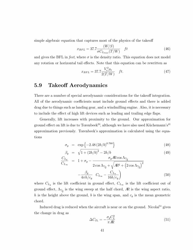
simple algebraic equation that captures most of the physics of the takeoff
xBFL = 37.7(W/S)
σCLmax(T/W )ft (46)
and gives the BFL in feet, where σ is the density ratio. This equation does not model
any rotation or horizontal tail effects. Note that this equation can be rewritten as
xBFL = 37.7V 2s ρo
2(T/W )ft. (47)
5.9 Takeoff Aerodynamics
There are a number of special aerodynamic considerations for the takeoff integration.
All of the aerodynamic coefficients must include ground effects and there is added
drag due to things such as landing gear, and a windmilling engine. Also, it is necessary
to include the effect of high lift devices such as leading and trailing edge flaps.
Generally, lift increases with proximity to the ground. Our approximation for
ground effect on lift is due to Torenbeek24, although we have also used Kuchemann’s41
approximation previously. Torenbeek’s approximation is calculated using the equa-
tions
σg = exp{−2.48 (2h/b)0.768
}(48)
βg =√
1 + (2h/b)2 − 2h/b (49)
CLgCL∞
= 1 + σg −σgAR cos Λc/2
2 cos Λc/2+
√AR2 +
(2 cos Λc/2
)2
− βg4πh/cg
(CL∞ −
CLα16h/cg
)(50)
where CLg is the lift coefficient in ground effect, CL∞ is the lift coefficient out of
ground effect, Λc/2is the wing sweep at the half chord, AR is the wing aspect ratio,
h is the height above the ground, b is the wing span, and cg is the mean geometric
chord.
Induced drag is reduced when the aircraft is near or on the ground. Nicolai51 gives
the change in drag as
∆CDi = −σgC2L
πAR(51)
41

where σg is calculated using Eq. (48).
The landing gear remains extended for the entire takeoff. It is necessary to include
this contribution to the total drag when analyzing takeoff. For preliminary design,
Torenbeek24 suggests using
CDlg = C1W 0.785
S
[1− 0.04
CLS
`mgb
]2
(52)
where `mg is the length of the main gear, and C1 is 4.05× 10⁻³ for English units, and
7.0× 10⁻⁴ for metric measurements.
When an engine fails, not only is the thrust of that engine lost, but there is an
increase in drag due to the windmilling engine. This increment in drag is calculated
using
CDwm =1
S
[0.1πr2
i +2
1 + 0.16M2AN
VNV
(1− VN
V
)](53)
from Ref. [24]. In this equation, ri is the engine inlet radius, AN is the nozzle area,
and VNV
is the ratio of the nozzle velocity to the airspeed velocity. Torenbeek suggests
using VNV
= 0.42 for low bypass ratio engines with mixed flow.
High lift devices are critically important for efficient low speed operation of an
HSCT. Antani52 discusses the requirements and issues for high lift systems for an
HSCT. Neglecting the effects of the high lift systems would lead to unrealistic designs
with low wing loading and poor overall performance, as the supersonic efficiency would
have to be drastically compromised to satisfy the field performance requirements.
Benoliel53 provides a survey of data for many different HSCT type planforms, and
Baber54 provides very detailed data on the AST-105-1 configuration. Data from these
sources was used to add lift and moment flap effects for our configuration. Specifically,
for the longitudinal derivatives with respect to flap deflection, we assume
CLδf = 0.2508 (54)
CMδf= −0.0550 (55)
and these values are fixed throughout the optimization. This results in
∆CL = CLδf δf = 0.2508δf
∆CM = CMδfδf = −0.0550δf .
42

We are currently assuming a takeoff flap deflection of 30◦. We neglect changes in drag
due to flap deflection.
5.10 Powered Approach Trim
The powered approach trim requirement involves calculating the pitching moment
about the cg, in the approach configuration. In this case the net pitching moment
should be zero. This is given by
Mcg = TzTcg + qSCDzDcg − qSCLxLcg + qScCM = 0 (56)
which can be rewritten as
CM =1
c
(CLxLcg − CD
(zTcg + zDcg
)− W sinα
qSzTcg
)(57)
where α is the landing angle of attack, which is calculated assuming that L = W .
Equation (57) is the pitching moment generated by the lift, drag, thrust, and weight.
The pitching moment to balance this, as given by Etkin55 is
CM = CMαα+ CMHT(58)
or
CM = CMαα + CLαHT VHit
[1−
CLαHT SHT
CLαS
(1− dε
dα
)](59)
where VH is the horizontal tail volume coefficient, and ε is the downwash angle. This
can be solved for the horizontal tail deflection, it,
it =CM − CMαα
CLαHT VH
[1− CLαHT
SHT
CLαS
(1− dε
dα
)] (60)
Substituting the pitching moment calculated in Eq. (57) into Eq. (60) gives the re-
quired tail deflection. This analysis neglects the effects of flaps.
43

5.11 Engine Scaling
Modern high thrust, high bypass ratio engines have fan diameters of over 10 ft. Al-
though the HSCT will not use engines with fans this large, thrust requirements can
rapidly increase the size of the engine. As engine size increases, so does the weight
and the drag on the nacelle. Engine size is largely determined by the mass flow of air
required for a given bypass ratio. The thrust is highly dependent on the mass flow
through the engine. We assume that the thrust is directly proportional to the mass
flow.T
Tref=
m
mref(61)
With this, we can scale the engine nacelle size directly from thrust using equations
from Nicolai51:
Dnac
Dnacref
=
√T
Tref(62)
lnaclnacref
=
√T
Tref(63)
where Dnac and lnac are the diameter and length of the nacelle.
Thrust is also used to calculate the weight of the engine in the FLOPS11 weight
routineWeng
Wengref
=
(T
Tref
)seng(64)
We use seng = 1.081 in the equation.
5.12 Minimum Time Climb with Dynamic Pres-
sure Constraint
To investigate the effect of climb requirements, we added a minimum time climb to
transition from the subsonic leg to the supersonic leg. The minimum time climb is
calculated using the energy approach as described by Rutowski56 and Bryson et al.57.
In this approach, the specific excess power,
Ps =(T −D)V
W(65)
44

0.5 1.0 1.5 2.0 2.5
10000
20000
30000
40000
50000
60000
70000
1
1
1
2
2
2
3
3
3
4
4
4
4 4
5
5
5
5
6
6
6
6
7
7
7
7
7
8
8 8
8
8
99
9
9
9
A
A
A
B
B
C
C
D
D
E
E
F
G
G
H
H
I
I J
Level Ps
J 300I 290H 280G 275F 250E 225D 200C 175B 150A 1409 1308 1257 1206 1105 1004 753 502 251 0
0.5 1.0 1.5 2.0 2.5
10000
20000
30000
40000
50000
60000
70000
10000
20000
30000
40000
50000
60000
7000080000
90000
110000
120000
130000140000
100000
0.5 1.0 1.5 2.0 2.5
10000
20000
30000
40000
50000
60000
70000
500
1000
1500
2000
2500
3000
Alti
tude
(ft
)
Mach number
q =
Figure 11: Specific excess power contours for a HSCT configuration
is maximized for a constant energy height,
he = h+V 2
2g. (66)
This is done by varying the speed, V , and at each speed and altitude calculating
thrust (T ) and drag (D). To efficiently find the maximum, we use a routine which
combines a golden section search with parabolic interpolation. This can be done
for a range of energy heights and will calculate the minimum time climb flight path
for the aircraft. Often, the optimum flight path would require the aircraft to fly
at unrealistically high dynamic pressures. We must place a limit on the maximum
allowable dynamic pressure, which limits the flight path.
Figure 11 shows a plot of specific excess power curves with lines of constant energy
height ranging from 10,000 ft to 150,000 ft and constant dynamic pressure ranging
from 500 psf to 3,000 psf. Due to structural considerations, we limit the maximum
dynamic pressure to be 1,000 psf. This eliminates much of the region shown in Fig. 11,
and for this aircraft the minimum time climb would be along the q = 1000 psf curve.
45

5.13 Optimization Strategies
Most optimizations of complex engineering systems replace the objective function
and/or constraints with easy-to-calculate approximations. The optimum of the ap-
proximate problem is found and then the approximation is updated in the neigh-
borhood of this optimum and the process repeated. The sequential linear program-
ming used for the structural optimization is the simplest form of such sequential
approximate optimization—it employs linear approximations. For the overall design
we employ sequential approximate optimization using the VCM approximation de-
scribed earlier. The numerical optimization is performed using the NEWSUMT-A
program58 which employs an extended interior penalty function. Newton’s method
with approximate second derivatives is used for unconstrained minimization.
During the typical optimization process the move limits on the variables were se-
lected to avoid excessive errors in the approximations. Typical initial move limits were
approximately fifteen percent, and they were decreased throughout the optimization
process to approximately two percent as the optimization neared completion.
46

Chapter 6
Results
In this chapter, we describe the results of a number of optimization runs. First, we
will discuss a case with no vertical or horizontal tail sizing. Then, two cases with
vertical tail sizing using slightly different starting conditions are presented, followed
by two cases with vertical and horizontal tail sizing. The second case shows the effect
of engine technology. Then we discuss a case with engine sizing and a case with all of
the above and a subsonic leg added to our mission. Table 6 lists the cases and charts
the progression of the cases. These cases show the difficulties in optimizing, as well
as the successes.
Table 6: Overview of results
+ New + Engine sizingCase Basic + VT + HT engine (new engine) + Subsonic leg26a X27a X27b X ←− −→28a X28b X
29a︷ ︸︸ ︷Shows effect X
29b of engine technology X
47

6.1 Baseline Optimization (Case 26a)
This optimization, case 26a, is used as a control case. It allows us to determine
the effects of the changes we make. It has 26 design variables, and 62 constraints.
Constraints numbered 47-52, 69 and 70 in Table 2 were not used in this case. The
mission is entirely supersonic, the vertical tail is fixed in both size and shape, and
there is no horizontal tail.
The initial design violated three constraints, the range constraint and the two
thrust constraints. After 30 optimization cycles, the TOGW has been reduced by
34,200 lbs with all of the constraints satisfied. A convergence history of the TOGW
is shown in Fig. 12. The initial and final planforms are shown in Figure 13 and Table
7 compares the two designs.
The final design has an unusual planform, with the inboard trailing edge swept
forward. The optimizer moved immediately to this design, and as can be seen in
Figure 14 the wing weight is reduced by about 14,000 lbs. Due to the lower aspect
ratio, the drag due to lift does increase, Fig. 15, but this is offset by a reduction in
volumetric wave drag, shown in Figure 16. Overall, the total drag decreases slightly
by the end of the optimization, Fig. 17.
The initial design has a wing loading of 63.68 psf. In the final design the wing
loading has been reduced to 56.30 psf. Lowering the aspect ratio improves the super-
sonic efficiency, but it also lowers the lift curve slope. This means that for a given
wing area, the aircraft would have to fly at a higher angle of attack to generate the
same lift. To keep from violating the 12◦ angle of attack constraint the optimizer
increased the wing area, which decreased the wing loading.
6.2 Vertical Tail Considerations
These optimizations include the vertical tail sizing, and require 27 design variables
with 64 constraints. Constraint number 66 is changed to the engine out limit from
the arbitrary limit of 50% of the semispan, and constraints 47 and 48 are added for
the crosswind landing. Again, the mission is entirely supersonic, and there is no
48

540000
550000
560000
570000
580000
590000
600000
610000
5200
5250
5300
5350
5400
5450
5500
5550
0 5 10 15 20 25 30
GTOW
CGTOW
Range
Wei
ght (
lbs) R
ange (nm)
Cycle
Figure 12: Convergence of Case 26a
0 50 100 150 200 250 3000
20
40
60
80
ft
0 50 100 150 200 250 3000
20
40
60
80
ft
0 50 100 150 200 250 3000
20
40
60
80
ft
Final Design
0 50 100 150 200 250 3000
20
40
60
80
ft
Initial Design
Figure 13: Initial and final planforms, Case 26a
49

Table 7: Comparison of Initial and Final Designs, Case 26a
Initial FinalGross Weight (lbs) 580,000 545,800Fuel Weight (lbs) 290,900 273,600Fuel Wt / Gross Wt 50.2% 50.1%Wing Area (ft2) 9,108 9,693Wing Weight (lbs) 81,900 68,070Aspect Ratio 2.36 1.59Range (n.mi.) 5,260.0 5,494.6Landing angle of attack 11.35◦ 11.99◦
(L/D)max 9.473 9.588
60000
65000
70000
75000
80000
85000
-50
-40
-30
-20
-10
0
0 5 10 15 20 25 30
Win
g W
eigh
t (lb
s)
Inboard TE
sweep angle (deg)
Cycle
Weight
Sweep angle
Figure 14: History of wing weight and trailing edge sweep, Case 26a
50

0.0053
0.0054
0.0055
0.0056
0.0057
0.0058
0 5 10 15 20 25 30
CD
lift
Cycle
Figure 15: History of drag due to lift, at CL = 0.1, Case 26a
0.0010
0.0011
0.0012
0.0013
0.0014
0.0015
0 5 10 15 20 25 30
CD
wav
e
Cycle
Figure 16: History of wave drag, Case 26a
51

0.0102
0.0103
0.0104
0.0105
0.0106
0.0107
0 5 10 15 20 25 30
CD
Cycle
Figure 17: History of total drag, at CL = 0.1, Case 26a
horizontal tail, but the vertical tail is allowed to vary in size.
6.2.1 Case 27a
The same initial design is used as in Case 26a, with the exception that the initial
value of the starting altitude was changed from 50,000 ft to 60,000 ft, and the climb
rate was changed from 100 ft/sec to 50 ft/sec. These changes increased the range
by over 80 n.mi. In addition to the three constraint violations mentioned previously,
the engine out limit is violated. The engines are too far out for the vertical tail to
trim in an emergency. After 30 optimization cycles, the TOGW has been reduced by
32,700 lbs with all of the constraints satisfied. A convergence history of the TOGW
is shown in Fig. 18. The initial and final planforms are shown in Figure 19 and Table
8 compares the two designs.
The vertical tail initially increased in size to satisfy the engine out constraint, but
was reduced as the engines continued to move inboard, see Fig. 20. In this case, more
weight is saved by moving the engines in and reducing the vertical tail size than by
taking advantage of wing bending moment relief to reduce the wing weight. In the
final design, the engines are moved in as far as the constraints allow. This results in
a slightly heavier wing compared to Case 26a. But this also allows a small vertical
tail to be used to satisfy the engine out constraint. The weight penalty for going to
52

530000
540000
550000
560000
570000
580000
590000
5250
5300
5350
5400
5450
5500
5550
0 5 10 15 20 25 30
TOGWCTOGW
Range
Wei
ght (
lbs)
Range (n.m
i.)
Cycle
Figure 18: Convergence of Case 27a
0 50 100 150 200 250 3000
20
40
60
80
ft
0 50 100 150 200 250 3000
20
40
60
80
ft
0 50 100 150 200 250 3000
20
40
60
80
ft
Final Design
0 50 100 150 200 250 3000
20
40
60
80
ft
Initial Design
Figure 19: Initial and final planforms, Case 27a
53

Table 8: Comparison of Initial and Final Designs, Case 27a
Initial FinalGross Weight (lbs) 580,000 547,300Fuel Weight (lbs) 290,900 272,800Fuel Wt / Gross Wt 50.2% 49.8%Wing Area (ft2) 9,108 9,808Wing Weight (lbs) 81,900 70,060Aspect Ratio 2.36 1.57Vertical Tail Area (ft2) 450.0 431.0Vertical Tail Weight (lbs) 1,730 1,640Nacelle 1 position, y (ft) 17.8 9.4Nacelle 2 position, y (ft) 32.1 17.6Range (n.mi.) 5,342.4 5,493.4Landing angle of attack 11.35◦ 11.99◦
(L/D)max 9.239 9.577
this design is very small, about 0.27% of the TOGW.
The stability and control derivatives were estimated using the interlacing tech-
nique. This technique worked well, as shown in Figures 21 and 22. The jumps that
occur every five cycles are the updated derivatives from Kay’s code. The estimations
for Clβ show the greatest differences, although the magnitude of the jumps is not
larger than the jumps in the other derivatives.
6.2.2 Case 27b
It seemed odd that the optimizer moved the engines inboard, which reduces the
wing bending moment relief, resulting in a heavier wing. So we performed a second
optimization, Case 27b, using the same initial design as Case 27a, but we started with
a larger vertical tail. There was initially no violation of the engine out constraint.
This allowed the engines to remain well outboard where there is a larger wing bending
moment relief effect.
The optimal design occurred after only 11 optimization cycles, but due to noisy
derivatives, the optimizer slowly wandered away from this design. The optimal design
54

5
10
15
20
25
30
35
350
400
450
500
550
600
650
0 5 10 15 20 25 30
Nacelle 1Nacelle 2
Vertical tail area
Span
wis
e na
celle
pos
ition
(ft
)
Vertical tail area (ft 2)
cycle
Figure 20: History of nacelle positions and vertical tail area
has a TOGW of 543,700 lbs, a reduction of 37,700 lbs from the initial design. The
initial and final planforms are shown in Figure 23 and Table 9 compares the two
designs.
The range decreased by 100 n.mi. when the vertical tail size was increased by
400 ft2. This is due to the increased drag from the larger tail. Although this seems
like a large penalty, the final design is slightly better than the Case 27a final design.
The nacelles are split because the vertical tail must balance the net yawing moment.
Thus, the net yawing moment will remain the same by moving nacelle 1 in and nacelle
2 out by equal distances. These cases show our derivative based optimization is very
susceptible to local minima. Also, these two cases indicate that nacelle position is not
a design driver and nacelles can be placed using other considerations, such as landing
gear interference with inlet flow or rotor burst.
The stability and control derivatives are well estimated for this case. Although
there is a large jump after the initial five cycles, the approximate analysis agrees well
with the detailed estimations after this. The history of the derivatives is shown in
Figures 24 and 25.
The most critical constraints for the final design are range and the engine out con-
straint. Some of the section C` constraints and the landing angle of attack constraint
are also critical. Also important in this design is fuel volume, nacelle strike on the
inboard nacelle, and minimum wing t/c.
55

-0.080
-0.075
-0.070
-0.065
-0.060
-0.055
-0.050
0 5 10 15 20 25 30
Cyb
eta
Cycle
-0.0005
0.0000
0.0005
0.0010
0.0015
0.0020
0.0025
0.0030
0.0035
0 5 10 15 20 25 30
Clb
eta
Cycle
0.030
0.035
0.040
0.045
0.050
0.055
0 5 10 15 20 25 30
Cnb
eta
Cycle
Figure 21: History of Cyβ , Clβ , and Cnβ for Case 27a
56

0.035
0.040
0.045
0.050
0.055
0.060
0 5 10 15 20 25 30
Cyd
r
Cycle
-0.0060
-0.0055
-0.0050
-0.0045
-0.0040
-0.0035
-0.0030
0 5 10 15 20 25 30
Cld
r
Cycle
-0.055
-0.050
-0.045
-0.040
-0.035
-0.030
0 5 10 15 20 25 30
Cnd
r
Cycle
Figure 22: History of Cyδr , Clδr , and Cnδr for Case 27a
57
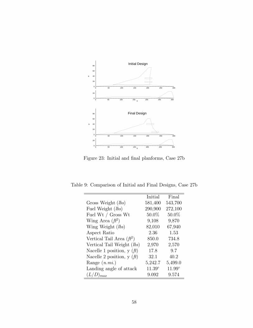
0 50 100 150 200 250 3000
20
40
60
80
100
ft
0 50 100 150 200 250 3000
20
40
60
80
100
ft
0 50 100 150 200 250 3000
20
40
60
80
ft
Final Design
0 50 100 150 200 250 3000
20
40
60
80
ft
Initial Design
Figure 23: Initial and final planforms, Case 27b
Table 9: Comparison of Initial and Final Designs, Case 27b
Initial FinalGross Weight (lbs) 581,400 543,700Fuel Weight (lbs) 290,900 272,100Fuel Wt / Gross Wt 50.0% 50.0%Wing Area (ft2) 9,108 9,870Wing Weight (lbs) 82,010 67,940Aspect Ratio 2.36 1.53Vertical Tail Area (ft2) 850.0 734.8Vertical Tail Weight (lbs) 2,970 2,570Nacelle 1 position, y (ft) 17.8 9.7Nacelle 2 position, y (ft) 32.1 40.2Range (n.mi.) 5,242.7 5,499.0Landing angle of attack 11.39◦ 11.99◦
(L/D)max 9.092 9.574
58
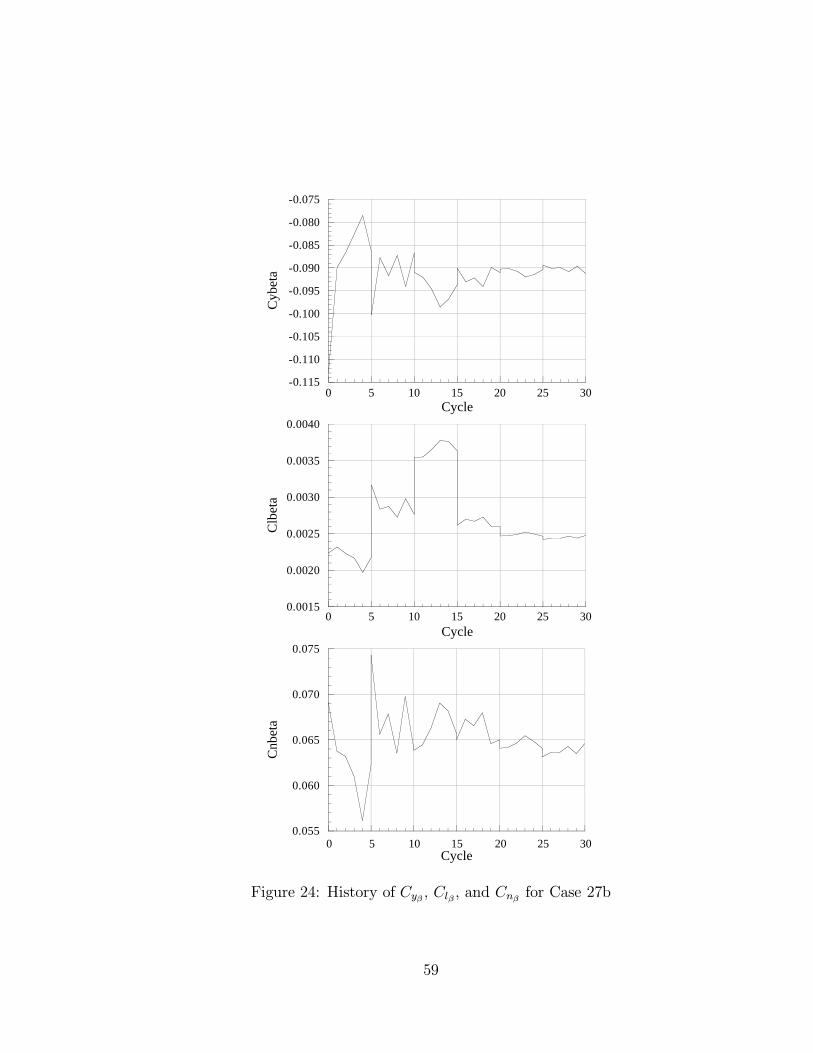
-0.115
-0.110
-0.105
-0.100
-0.095
-0.090
-0.085
-0.080
-0.075
0 5 10 15 20 25 30
Cyb
eta
Cycle
0.0015
0.0020
0.0025
0.0030
0.0035
0.0040
0 5 10 15 20 25 30
Clb
eta
Cycle
0.055
0.060
0.065
0.070
0.075
0 5 10 15 20 25 30
Cnb
eta
Cycle
Figure 24: History of Cyβ , Clβ , and Cnβ for Case 27b
59

0.065
0.070
0.075
0.080
0.085
0 5 10 15 20 25 30
Cyd
r
Cycle
-0.0074
-0.0072
-0.0070
-0.0068
-0.0066
-0.0064
-0.0062
-0.0060
-0.0058
0 5 10 15 20 25 30
Cld
r
Cycle
-0.078
-0.076
-0.074
-0.072
-0.070
-0.068
-0.066
-0.064
0 5 10 15 20 25 30
Cnd
r
Cycle
Figure 25: History of Cyδr , Clδr , and Cnδr for Case 27b
60

6.3 Vertical and Horizontal Tail Considerations
Next, we added horizontal tail sizing to our optimization. This increased the number
of design variables to 28 and the number of constraints to 67. The constraints added
are the takeoff rotation constraint, the approach trim constraint and a constraint to
prevent the wing and horizontal tail from overlapping.
6.3.1 Case 28a
The starting design from Case 27a is used, with the addition of a horizontal tail.
Adding the horizontal tail only increased the weight by 9,000 lbs, but the additional
drag caused a 400 n.mi. reduction in the range. This design satisfies the three addi-
tional constraints for the horizontal tail.
The weight of the final design is 630,000 lbs, an increase of over 40,000 lbs from
the starting weight, and more than 80,000 lbs heavier than the previous optimized
designs. Most of this weight increase is fuel weight. Almost 70,000 lbs more fuel
is required for this design than for Case 27a. The planforms are all very similar,
although the trailing edge is somewhat less swept in this case.
The initial and final planforms are shown in Figure 26 and Table 10 compares
the two designs. The convergence histories of the TOGW, vertical tail size and
nacelle locations, and horizontal tail size are shown in Figures 27, 28, 29. The noisy
convergence is a product of our variable complexity modeling and the noisy analysis.
For the final design, range and landing angle of attack are again the critical con-
straints. There are a number of constraints which were important, but not critical,
to this design. These include fuel volume, section C`, time required to rotate, mini-
mum nacelle spacing, the engine out limit, and maximum thrust required during the
cruise-climb.
6.3.2 Case 28b
We performed another optimization using the same initial design variables, but in-
creasing the size and thrust of the engines to see the effects of engine technology.
61

0 50 100 150 200 250 3000
10
20
30
40
50
60
70
80
90
0 50 100 150 200 250 3000
10
20
30
40
50
60
70
80
90
0 50 100 150 200 250 3000
10
20
30
40
50
60
70
80
90
Initial Design
ft
0 50 100 150 200 250 3000
10
20
30
40
50
60
70
80
90
Final Design
Figure 26: Initial and final planforms, Case 28a
Table 10: Comparison of Initial and Final Designs, Case 28a
Initial FinalGross Weight (lbs) 589,200 630,000Fuel Weight (lbs) 290,900 340,200Fuel Wt / Gross Wt 50.0% 54.0%Wing Area (ft2) 9,108 9,713Wing Weight (lbs) 82,630 77,720Aspect Ratio 2.36 1.95Vertical Tail Area (ft2) 450.0 447.1Vertical Tail Weight (lbs) 1,740 1,760Nacelle 1 position, y (ft) 17.8 9.4Nacelle 2 position, y (ft) 32.1 17.1Horz. Tail Area (ft2) 1,500.0 1,400.1Horz. Tail Weight (lbs) 7,930 7,510Time to rotate (sec) 4.56 4.67Range (n.mi.) 4,935.9 5,465.2Landing angle of attack 11.27◦ 11.97◦
(L/D)max 8.709 8.711
62
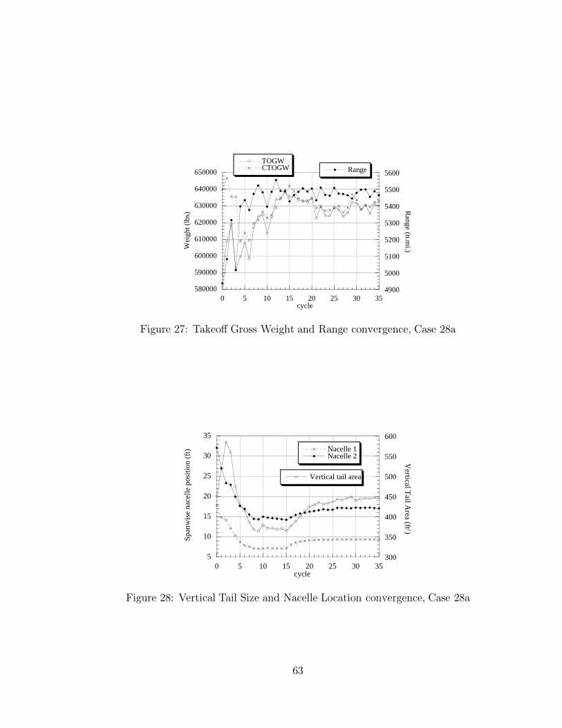
580000
590000
600000
610000
620000
630000
640000
650000
4900
5000
5100
5200
5300
5400
5500
5600
0 5 10 15 20 25 30 35
TOGWCTOGW Range
Wei
ght (
lbs)
Range (n.m
i.)
cycle
Figure 27: Takeoff Gross Weight and Range convergence, Case 28a
5
10
15
20
25
30
35
300
350
400
450
500
550
600
0 5 10 15 20 25 30 35
Nacelle 1Nacelle 2
Vertical tail area
Span
wis
e na
celle
pos
ition
(ft
)
Vertical T
ail Area (ft 2)
cycle
Figure 28: Vertical Tail Size and Nacelle Location convergence, Case 28a
63

620
640
660
680
700
720
740
760
780
0 5 10 15 20 25 30 35
Hor
izon
tal T
ail A
rea
(ft2
)
cycle
Figure 29: Horizontal Tail Size convergence, Case 28a
Engine thrust increased from 39,000 lbs to 46,000 lbs per engine, nacelle diameter and
length increased from 5 ft and 27 ft to 6.5 ft and 35 ft, respectively. The engine thrust
to weight ratio was reduced by 1, which increased the propulsion system weight by
over 28,000 lbs and the TOGW by about 35,600 lbs. Also, the range decreased by
436 n.mi., although the drag on the aircraft only increased by about two counts. The
initial weight of this design is only about 5,000 lbs less than the optimized design in
the previous case. The range is 1,000 n.mi. less than our required range.
After 40 optimization cycles, our TOGW is 755,400 lbs. Although this could be
a poor local minimum, this large increase is weight can be explained. With no other
changes, the large range deficiency would require approximately 100,000 lbs of fuel
to satisfy the range constraint. Adding this much fuel weight would cause numerous
other constraint violations, such as the thrust constraints, the fuel volume constraint,
the landing angle of attack, and the takeoff rotation constraint. Satisfying these
constraints would further increase the weight. The actual increase in fuel weight is
about 118,000 lbs.
The final planform is very similar to our previous designs, but the wing is much
bigger. The initial and final planforms are shown in Figure 30. These designs are also
compared in Table 11. In this design, range, landing angle of attack, section C`, and
the engine out limit are the critical constraints. Once again, fuel volume, inboard
64

0 50 100 150 200 250 3000
10
20
30
40
50
60
70
80
90
0 50 100 150 200 250 3000
10
20
30
40
50
60
70
80
90
0 50 100 150 200 250 3000
10
20
30
40
50
60
70
80
90
Final Design
0 50 100 150 200 250 3000
10
20
30
40
50
60
70
80
90
Initial Design
Figure 30: Initial and final planforms, Case 28b
Table 11: Comparison of Initial and Final Designs, Case 28b
Initial FinalGross Weight (lbs) 624,800 755,400Fuel Weight (lbs) 290,900 408,600Fuel Wt / Gross Wt 50.0% 54.0%Wing Area (ft2) 9,108 11,193Wing Weight (lbs) 84,300 95,800Aspect Ratio 2.36 2.08Vertical Tail Area (ft2) 450.0 564.6Vertical Tail Weight (lbs) 1,770 2,270Nacelle 1 position, y (ft) 17.8 10.1Nacelle 2 position, y (ft) 32.1 19.5Horz. Tail Area (ft2) 1,500.0 1,647.1Horz. Tail Weight (lbs) 8,030 9,150Time to rotate (sec) 4.47 4.68Range (n.mi.) 4,500.6 5,471.9Landing angle of attack 12.26◦ 12.00◦
(L/D)max 8.573 8.684
65

nacelle strike, time to rotate, and maximum thrust required for cruise-climb are the
other important constraints.
6.4 Engine Sizing (Case 29a)
Our next optimization included engine sizing, as well as the vertical and horizontal
tail sizing. This added one design variable, up to 29, and one constraint, up to 68.
The balanced field length constraint of 10,000 ft is the additional constraint. Cases
28a and 28b both violate this constraint considerably with balanced field lengths of
11,650.9 ft and 12794.3 ft, respectively. The initial design for this case is the final
design from case 28b.
The final design is much heavier than the initial design. The weight increases by
110,000 lbs. The final design has a much larger wing. Wing area increases by 1,569 ft
and wing weight increases by over 33,000 lbs. Increasing the wing area often reduces
the wing loading, which decreases the balanced field length, but in this case, the wing
loading increases from 59.04 lbs/ft2 to 60.22 lbs/ft2. This is a relatively small increase
in wing loading and it allows a smaller, lighter wing to be used.
To satisfy the balanced field length constraint the thrust to weight ratio is in-
creased by 13.5%, from 0.244 to 0.277. This is accomplished by increasing the thrust
per engine by almost 14,000 lbs. Increasing the thrust causes the propulsion system
weight to increase by almost 25,000 lbs. Clearly, the balanced field length constraint
was a critical requirement. Relaxing the BFL constraint to 11,000 ft would result in
a considerable weight savings.
For the final design, the constraints on range, nacelle strike, BFL, and the engine
out condition were all critical. The nacelle strike constraint is limiting the landing
angle of attack in this case. The BFL constraint sizes the engine, and the engine
out condition sizes the vertical tail. The constraints on maximum thrust required,
section C`, time to rotate, and horizontal tail/wing overlap were nearly critical. The
horizontal tail is sized by the time to rotate constraint.
The initial and final planforms are shown in Figure 31 and the designs are com-
pared in Table 12. The convergence is very noisy between cycles 10 and 30, but is
66

0 50 100 150 200 250 3000
10
20
30
40
50
60
70
80
90
0 50 100 150 200 250 3000
10
20
30
40
50
60
70
80
90
0 50 100 150 200 250 3000
10
20
30
40
50
60
70
80
90
Initial Design
0 50 100 150 200 250 3000
10
20
30
40
50
60
70
80
90 Final Design
Figure 31: Initial and final planforms, Case 29a
good for cycles 30 to 45 as can be seen in Figure 32. Figure 33 shows the history of
the balanced field length.
6.5 Subsonic Leg (Case 29b)
For this optimization, we added a subsonic leg to our mission requirement. We re-
quired the initial 500 n.mi. be flown at Mach 0.9 and then continue on with the
supersonic cruise-climb. This did not add any design variables, but did require two
more constraints. The additional constraints require that the available thrust be
greater than the required thrust for the subsonic leg and the transition from the sub-
sonic to supersonic leg. In this optimization, the transition is an instantaneous jump.
The addition of these constraints results in 29 design variables and 70 constraints.
The initial design for this case is the final design from Case 29a. After adding the
subsonic leg to the mission, the range for this design dropped to 5,221.5 n.mi., a 280
n.mi. decrease. The range constraint is the only constraint which is initially violated.
The optimizer had trouble improving the range without violating the BFL con-
straint. Many attempts were made using different move limits to find a design which
67
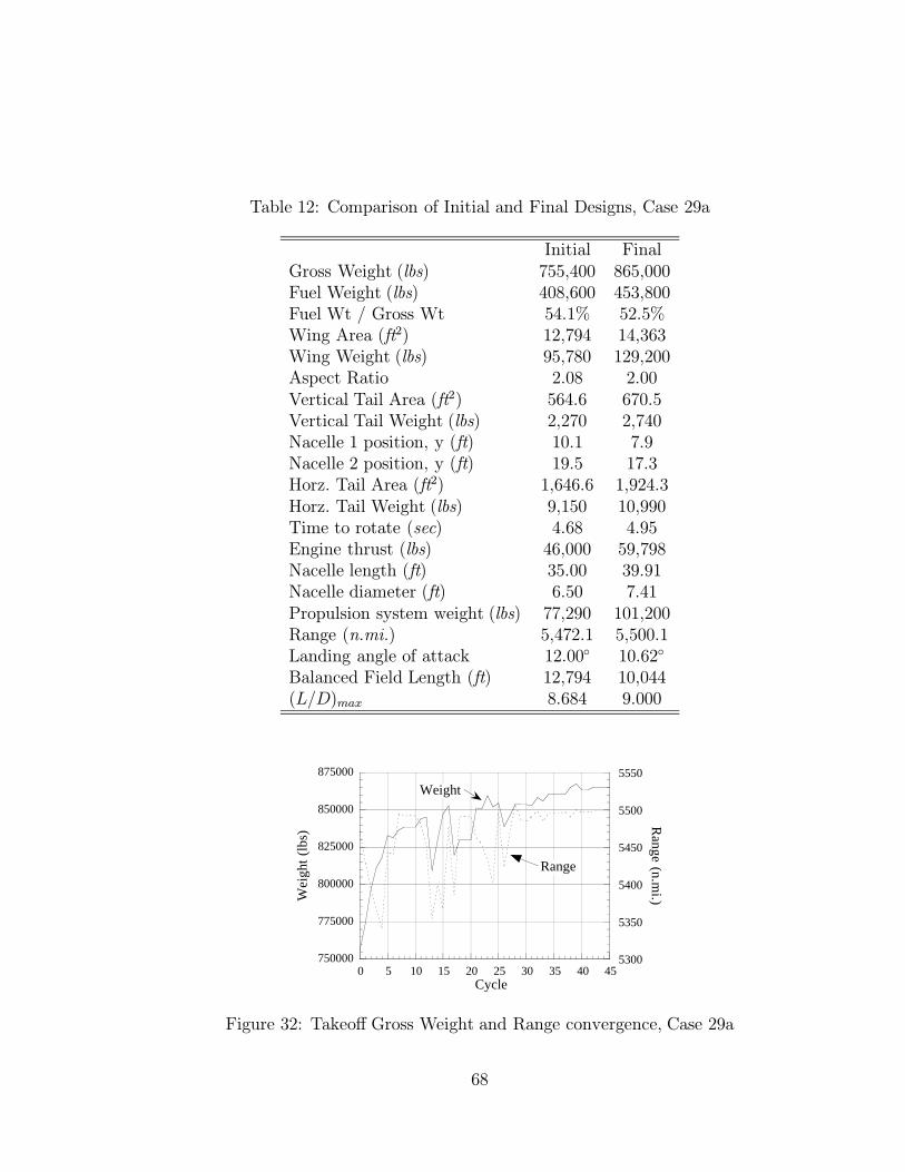
Table 12: Comparison of Initial and Final Designs, Case 29a
Initial FinalGross Weight (lbs) 755,400 865,000Fuel Weight (lbs) 408,600 453,800Fuel Wt / Gross Wt 54.1% 52.5%Wing Area (ft2) 12,794 14,363Wing Weight (lbs) 95,780 129,200Aspect Ratio 2.08 2.00Vertical Tail Area (ft2) 564.6 670.5Vertical Tail Weight (lbs) 2,270 2,740Nacelle 1 position, y (ft) 10.1 7.9Nacelle 2 position, y (ft) 19.5 17.3Horz. Tail Area (ft2) 1,646.6 1,924.3Horz. Tail Weight (lbs) 9,150 10,990Time to rotate (sec) 4.68 4.95Engine thrust (lbs) 46,000 59,798Nacelle length (ft) 35.00 39.91Nacelle diameter (ft) 6.50 7.41Propulsion system weight (lbs) 77,290 101,200Range (n.mi.) 5,472.1 5,500.1Landing angle of attack 12.00◦ 10.62◦
Balanced Field Length (ft) 12,794 10,044(L/D)max 8.684 9.000
750000
775000
800000
825000
850000
875000
5300
5350
5400
5450
5500
5550
0 5 10 15 20 25 30 35 40 45
Wei
ght
(lbs
)
Range (n.m
i.)
Cycle
Range
Weight
Figure 32: Takeoff Gross Weight and Range convergence, Case 29a
68

9500
10000
10500
11000
11500
12000
12500
13000
0 5 10 15 20 25 30 35 40 45
BF
L (
ft)
Cycle
Figure 33: Balanced field length convergence, case 29a
would satisfy both constraints. The final design satisfies both constraints, but weighs
100,000 lbs more than the initial design.
Seventy percent of the increase in weight is due to added fuel. Another 20% of
the increase comes from increased wing weight. The rest of the weight increase comes
from various sources, including the vertical tail, horizontal tail, and the propulsion
system.
The final design does not appear too different from the initial design. There is
an increase in aspect ratio which improves the subsonic aerodynamic performance.
Figure 34 shows both the starting and ending designs and Table 13 compares them.
Convergence of TOGW, range, and BFL is shown in Figures 35 and 36.
The increase in weight agrees with trends predicted in other studies. A study
by the Douglas Aircraft Company59 showed large increases in weight with increasing
subsonic mission segments. Martin et al.60 also predicted increases in weight corre-
sponding to increasing subsonic leg.
The actual subsonic leg requirements for an HSCT could be less than the 500
n.mi. that we have used. Reducing this requirement would make it easier for the
optimizer to find a feasible design. An increase in the allowable BFL could also help
the optimizer.
69

0 50 100 150 200 250 3000
10
20
30
40
50
60
70
80
90
0 50 100 150 200 250 3000
10
20
30
40
50
60
70
80
90
0 50 100 150 200 250 3000
10
20
30
40
50
60
70
80
90 Initial Design
0 50 100 150 200 250 3000
10
20
30
40
50
60
70
80
90 Final Design
Figure 34: Initial and final planforms, Case 29b
860000
880000
900000
920000
940000
960000
980000
1000000
0 10 20 30 40
TO
GW
(lb
s)
Cycle
Figure 35: Takeoff Gross Weight convergence, Case 29b
70

Table 13: Comparison of Initial and Final Designs, Case 29b
Initial FinalGross Weight (lbs) 865,000 966,400Fuel Weight (lbs) 453,800 523,900Fuel Wt / Gross Wt 52.5% 54.2%Wing Area (ft2) 14,363 15,610Wing Weight (lbs) 129,200 148,900Aspect Ratio 1.99 2.18Vertical Tail Area (ft2) 670.5 778.2Vertical Tail Weight (lbs) 2,740 3,210Nacelle 1 position, y (ft) 7.9 11.0Nacelle 2 position, y (ft) 17.3 19.9Horz. Tail Area (ft2) 1,924.3 2,293.4Horz. Tail Weight (lbs) 10,990 13,400Time to rotate (sec) 4.95 4.86Engine thrust (lbs) 59,798 62,972Nacelle length (ft) 39.91 40.95Nacelle diameter (ft) 7.41 7.61Propulsion system weight (lbs) 101,200 107,200Range (n.mi.) 5,221.5 5,519.2Landing angle of attack 10.62◦ 10.25◦
Balanced Field Length (ft) 10,047 9,984(L/D)max 8.998 8.953
5200
5250
5300
5350
5400
5450
5500
5550
9600
9800
10000
10200
10400
10600
10800
11000
0 10 20 30 40
Ran
ge (
nm) B
FL
(ft)
Cycle
Range
BFL
Figure 36: Range and BFL convergence, case 29b
71

6.6 Minimum Time to Climb Calculation
We tried to optimize a design including a minimum time climb segment in the mission.
Although the analysis for the minimum time climb segment works, it was not robust
enough to use in an optimization. The optimizer repeatedly caused the routine to
crash. Work is underway to improve the analysis so it can be used in an optimization.
There are two main problems. First, the routine sometimes has trouble finding
the maximum specific excess power for a given energy height. This is due to the
multimodal nature of the specific excess power curve for a constant energy height.
There are usually two local maximums, one subsonic and the other supersonic. Most
of the time the supersonic maximum is above the dynamic pressure limit, but it is
necessary for the search routine to find both maximums to determine if the dynamic
pressure limit is active. We have broken the search into two regions, which generally
allows us to find both maximums, but because of noise in the analysis, the routine
has trouble switching from the subsonic maximum to the supersonic maximum.
The other problem is the possible large differences between the flight path calcu-
lated using the detailed analysis and the approximate analysis. This difference can
cause range discrepancies of over 1,000 n.mi. if the detailed and approximate analysis
transition from subsonic to supersonic at significantly different places.
Another consideration is computing time. Including the minimum time to climb
segment in the mission can double or triple the time required to calculate the range.
This calculation is sometimes performed more than one thousand times during an
optimization cycle. This causes a very large increase in the time required to optimize
a design.
72

Chapter 7
Conclusions
Multidisciplinary design optimization using variable complexity modeling can produce
feasible, optimized designs. We have extended and refined our code to explore design
issues which are not often considered at this level of aircraft design. We were not
successful in every case, but this may be due to unrealistic design requirements. A
summary of our optimization cases is shown in Table 14
We have added essential trim and control effects to our HSCT design methodology.
The variable complexity technique of interlacing the approximate stability derivative
predictions with the more accurate VLM predictions worked satisfactorily. Although
the derivatives were only updated with the VLM predictions once every 5 optimization
cycles, there was good agreement between the approximate predictions and the more
Table 14: Summary of optimizations
Case Addition Requirement Final Weight (lbs)26a None (baseline case) 545,80027a Vertical tail sizing 547,30027b Vertical tail sizing 543,70028a Horizontal tail sizing 630,00028b Reduced engine technology 755,40029a Balanced field length 865,00029b Subsonic leg 966,400
73

accurate predictions.
Adding the engine-out consideration forces the vertical tail to be sized based on
the engine location. We found that the spanwise engine location is constrained by
the aerodynamic control requirements. The engines are placed as far inboard as the
nacelle lateral spacing constraints allow, and the vertical tail size is minimized. But,
as was shown in Case 27b, there is another local minimum which has a larger vertical
tail and one nacelle located on the outboard wing section. This takes advantage of
the greater bending moment relief effect, which lowers the wing weight by about 2,000
lbs.
The inboard nacelle strike constraints were active in every case. In the first five
cases, it is not clear what these constraints affected. It is possible that these con-
straints limit the amount of trailing edge sweep in those cases. In the last two cases,
29a and 29b, these constraints limit the allowable landing angle of attack.
The horizontal tail size is based on the requirement that the aircraft must rotate
to the take-off position in under 5 sec. The tail size required to do this is highly
dependent on the positioning of the landing gear. The horizontal tail size is also very
sensitive to flap effects, which have only been crudely modeled in this work. The tail
deflection for approach trim was not critical for any of our designs.
The increased vertical tail size and the addition of a horizontal tail add less than
2.5% directly to the gross take-off weight, but they result in drag penalties, which
translate to large increases in weight. This increased weight is mostly fuel. The rest of
the weight increase is due to the greater amount of fuel being carried, not to structural
problems, which would be indicated by changes in the wing planform. Although we
found that trim and control increased the weight, adding these considerations provides
a more realistic model and better designs.
Reducing the technology level of the engines (∆T/W |eng = −1) caused a large
increase in engine weight and size. This caused a large decrease in range and a
large weight penalty was incurred to satisfy all the constraints. Engine sizing was
added along with a balanced field length requirement. Our requirement of a 10,000
ft balanced field length seems overly restrictive and causes a very large increase in
TOGW.
74

Adding a 500 n.mi. subsonic leg to our mission caused a large decrease in total
range. Overcoming this range deficit while maintaining the balanced field length
requirement was difficult. The final design was much heavier than the starting design.
Our subsonic leg could be too long. A study of routes and regulations might indicate
that the required subsonic leg is shorter than the 500 n.mi. that we required. Although
this design is extremely heavy, it demonstrates that our MDO technique is capable of
producing successful designs, even when faced with requirements that are somewhat
unrealistic.
There are many opportunities for future work. An investigation into the effects of
varying the balanced field length requirement and the subsonic leg length is necessary.
This would indicate the quality of our models for these requirements. Future work
will include estimation of flap effects using response surfaces. This will improve both
the horizontal tail sizing, and the balanced field length models. Also, integrating the
minimum time to climb routine with the optimization is necessary.
75

References
[1] Sobieszczanski-Sobieski, J., “Multidisciplinary Optimization of Engineering Sys-
tems: Achievements and Potential,” in Proceedings of an International Sem-
inar, Optimization: Methods and Applications, Possibilities and Limitations
(Bergmann, H. W., ed.), vol. 47 of Lecture Notes in Engineering, pp. 42–62,
Berlin, Germany: Springer-Verlag, 1989.
[2] Sobieszczanski-Sobieski, J., “Multidisciplinary Design Optimization: An Emerg-
ing New Engineering Discipline,” presented at The World Congress on Optimal
Design of Structural Systems, (Rio de Janeiro, Brazil), Aug. 1993.
[3] Sobieszczanski-Sobieski, J. and Haftka, R. T., “Multidisciplinary Aerospace De-
sign Optimization: Survey of Recent Developments,” AIAA Paper 96-0711, Jan.
1996.
[4] McGeer, T., “Wing Design for Minimum Drag and Practical Constraints,” Jour-
nal of Aircraft, vol. 21, pp. 879–886, Nov. 1984.
[5] Grossman, B., Strauch, G., Eppard, W. M., Gurdal, Z., and Haftka, R. T.,
“Integrated Aerodynamic/Structural Design of a Sailplane Wing,” Journal of
Aircraft, vol. 25, no. 9, pp. 855–860, 1988.
[6] Wakayama, S. and Kroo, I., “A Method for Lifting Surface Design using Nonlin-
ear Optimization,” AIAA Paper 90–3290, Sept. 1990.
[7] Gallman, J. W., Smith, S. C., and Kroo, I. M., “Optimization of Joined-Wing
Aircraft,” Journal of Aircraft, vol. 30, pp. 897–905, November-December 1993.
76

[8] Chang, I. C., Torres, F. J., Driscoll, F. P., and Van Dam, C. P., “Optimization
of Wing-Body Configurations by the Euler Equations,” AIAA Paper 94-1899,
June 1994.
[9] Tzong, G., Baker, M., Yalamanchili, K., and Giesing, J., “Aeroelastic Loads and
Structural Optimization of a High Speed Civil Transport Model,” AIAA Paper
94-4378, Sept. 1994.
[10] Borland, C. J., Benton, J. R., Frank, P. D., Kao, T. J., Mastro, R. A., and
Barthelemy, J.-F. M., “Multidisciplinary Design Optimization of a Commercial
Aircraft Wing—an Exploratory Study,” AIAA Paper 94-4305, Sept. 1994.
[11] McCullers, L. A., “Aircraft Configuration Optimization Including Optimized
Flight Profiles,” in Proceedings of Symposium on Recent Experiences in Mul-
tidisciplinary Analysis and Optimization (Sobieski, J., ed.), NASA CP-2327,
pp. 396–412, Apr. 1984.
[12] Scott, P. W., “Developing Highly Accurate Empirical Weight Estimating Rela-
tionships: Obstacles and Techniques,” SAWE Paper No. 2091, May 1992.
[13] Udin, S. V. and Anderson, W. J., “Wing Mass Formula for Subsonic Aircraft,”
Journal of Aircraft, vol. 29, no. 4, pp. 725–727, 1992.
[14] Torenbeek, E., “Development and Application of a Comprehensive Design-
Sensitive Weight Prediction Method for Wing Structures of Transport-Category
Aircraft,” Delft University Department of Aerospace Engineering Report LR–
693, Sept. 1992.
[15] Huang, X., Dudley, J., Haftka, R. T., Grossman, B., and Mason, W. H., “Struc-
tural Weight Estimation for Multidisciplinary Optimization of a High-Speed Civil
Transport,” to appear Journal of Aircraft, vol. 33, May-June 1996.
[16] Hutchison, M. G., Unger, E., Mason, W. H., Grossman, B., and Haftka, R. T.,
“Variable-Complexity Aerodynamic Optimization of a High Speed Civil Trans-
port Wing,” Journal of Aircraft, vol. 31, pp. 110–116, January-Febuary 1994.
77

[17] Hutchison, M. G., Huang, X., Mason, W. H., Haftka, R. T., and Grossman,
B., “Variable-Complexity Aerodynamic-Structural Design of a High-Speed Civil
Transport Wing,” AIAA Paper 92-4695, Sept. 1992.
[18] Hutchison, M. G., Mason, W. H., Grossman, B., and Haftka, R. T., “Aero-
dynamic Optimization of an HSCT Configuration Using Variable-Complexity
Modeling,” AIAA Paper 93-0101, Jan. 1993.
[19] Dudley, J., Huang, X., Haftka, R. T., Grossman, B., and Mason, W. H.,
“Variable-Complexity Interlacing of Weight Equation and Structural Optimiza-
tion for the Design of the High-Speed Civil Transport,” AIAA Paper 94-4377,
Sept. 1994.
[20] Sliwa, S. M., “Impact of Longitudinal Flying Qualities Upon the Design of a
Transport With Active Controls,” AIAA Paper 80-1570, 1980.
[21] Sliwa, S. M., “Sensitivity of Optimal Preliminary Design of a Transport to Op-
erational Constraints and Performance Index,” AIAA Paper 80-1895, Aug. 1980.
[22] Kay, J., Mason, W. H., Durham, W., and Lutze, F., “Control Authority Assess-
ment in Aircraft Conceptual Design,” AIAA Paper 93-3968, Aug. 1993.
[23] McCarty, C. A., Feather, J. B., Dykman, J. R., Page, M. A., and Hodgkinson,
J., “Design and Analysis Issues of Integrated Control Systems for High-Speed
Civil Transports,” NASA Contractor Report 186022, May 1992.
[24] Torenbeek, E., Synthesis of Subsonic Airplane Design. Delft University Press,
1982.
[25] FAA, Washington, DC, FAR Part 25.
[26] Ogburn, M. E., Foster, J. v., Pahle, J. W., Wilson, R. J., and Lackey, J. B., “Sta-
tus of the Validation of High-Angle-of-Attack Nose-Down Pitch Control Margin
Design guidelines,” AIAA Paper 93-3623, 1993.
78

[27] Craidon, C. B., “Description of a Digital Computer Program for Airplane Con-
figuration Plots,” NASA TM X-2074, 1970.
[28] Barnwell, R., “Approximate Method for Calculating Transonic Flow About Lift-
ing Wing-Body Configurations,” NASA TR R-452, pp. 58–61, Apr. 1976.
[29] Hutchison, M., Unger, E., Mason, W. H., Grossman, B., and Haftka, R.,
“Variable-Complexity Aerodynamic Optimization of an HSCT Wing Using
Structural Wing-Weight Equations,” AIAA Paper 92-0212, Jan. 1992.
[30] Eminton, E., “On the Minimisation and Numerical Evaluation of Wave Drag,”
Royal Aircraft Establishment Report AERO.2564, Nov. 1955.
[31] MacMillin, P. E., Dudley, J., Mason, W. H., Grossman, B., and Haftka, R. T.,
“Trim, Control and Landing Gear Effects in Variable-Complexity HSCT Design,”
AIAA Paper 94-4381, Sept. 1994.
[32] Harris, Jr., R. V., “An Analysis and Correlation of Aircraft Wave Drag,” NASA
TM X-947, 1964.
[33] Hutchison, M. G., Multidisciplinary Optimization of High-Speed Civil Transport
Configurations Using Variable-Complexity Modeling. PhD thesis, Virginia Poly-
technic Institute and State University, Blacksburg, Virginia, Mar. 1993.
[34] Hollenback, O. M. and Bloom, G. A., “Applications of a Parabolized Navier-
Stokes Code to an HSCT Configuration and Comparison to Wind Tunnel Test
Data,” AIAA Paper 93-3537, Aug. 1993.
[35] Carlson, H. W. and Miller, D. S., “Numerical Methods for the Design and Anal-
ysis of Wings at Supersonic Speeds,” NASA TN D-7713, 1974.
[36] Carlson, H. W. and Mack, R. J., “Estimation of Leading-Edge Thrust for Su-
personic Wings of Arbitrary Planforms,” NASA TP-1270, 1978.
[37] Cohen, D. and Friedman, M. D., “Theoretical Investigation of the Supersonic
Lift and Drag of Thin, Sweptback Wings with Increased Sweep near the Root,”
NACA TN-2959, June 1953.
79

[38] Hopkins, E. J. and Inouye, M., “An Evaluation of Theories for Predicting Turbu-
lent Skin Friction and Heat Transfer on Flat Plates at Supersonic and Hypersonic
Mach Numbers,” AIAA Journal, vol. 9, pp. 993–1003, June 1971.
[39] Diederich, F. W., “A Planform Parameter for Correlating Certain Aerodynamic
Characteristics of Swept Wings,” NACA TN-2335, 1951.
[40] Polhamus, E. C., “Prediction of Vortex-Lift Characteristics by a Leading-Edge-
Suction Analogy,” Journal of Aircraft, vol. 8, pp. 193–199, 1971.
[41] Kuchemann, D., The Aerodynamic Design of Aircraft. Pergamon Press, 1978.
[42] Whetstone, W. D., Engineering Analysis Language Reference Manual. Engineer-
ing Information System, Incorporated, July 1983.
[43] Barthelemy, J.-F. M., Wrenn, G. A., Dove, A. R., Coen, P. G., and Hall, L. E.,
“Supersonic Transport Wing Minimum Weight Design Integrating Aerodynamics
and Structures,” Journal of Aircraft, vol. 31, March-April 1994.
[44] Roskam, J., Airplane Design Part V: Component Weight Estimation. Kansas:
Roskam Aviation and Engineering Corporation, 1985.
[45] Hoak, D. E. et al., USAF Stability and Control DATCOM. Flight Control Divi-
sion, Air Force Flight Dynamics Laboratory, WPAFB, Ohio, 45433-0000, 1978.
Revised.
[46] Roskam, J., Methods for Estimating Stability and Control Derivatives of Con-
ventional Subsonic Airplanes. Kansas: Roskam Aviation and Engineering Cor-
poration, 1971.
[47] Heffley, R. K. and Jewell, W. F., “Aircraft Handling Qualities Data,” NASA
Contractor Report 2144, 1972.
[48] Razgonyaev, V. and Mason, W. H., “An Evaluation of Aerodynamic Prediction
Methods Applied to the XB-70 for Use in High Speed Aircraft Stability and
Control System Design,” AIAA Paper 95-0759, Jan. 1995.
80
[49] Powers, S. A., “Critical Field Length Calculations for Preliminary Design,” Jour-
nal of Aircraft, vol. 18, pp. 103–107, Febuary 1981.
[50] Loftin, Laurence K., J., Subsonic Aircraft: Evolution and the Matching of Size
to Performance. NASA Reference Publication 1060, Aug. 1980.
[51] Nicolai, L. M., Fundamentals of Aircraft Design. San Jose, CA: METS Inc, 1975.
[52] Antani, D. L. and Morgenstern, J. M., “HSCT High-Lift Aerodynamic Technol-
ogy Requirements,” AIAA Paper 92-4228, Aug. 1992.
[53] Benoliel, A. M. and Mason, W. H., “Pitch-Up Characteristics for HSCT Class
Planforms: Survey and Estimation,” AIAA Paper 94-1819, June 1994.
[54] Baber, Jr., H. T., “Characteristics of the Advanced Supersonic Technology AST-
105-1 Configured for Transpacific Range with Pratt and Whitney Aircraft Vari-
able Stream Control Engines,” NASA TM-78818, Mar. 1979.
[55] Etkin, B., Dynamics of Flight–Stability and Control. New York: John Wiley &
Sons, Inc., 1982.
[56] Rutowski, E. S., “Energy Approach to the General Aircraft Performance Prob-
lem,” Journal of Aeronautical Science, vol. 21, pp. 187–195, Mar. 1954.
[57] Bryson, Jr., A. E., Desai, M. N., and Hoffman, W. C., “Energy-State Approxima-
tion in Performance Optimization of Supersonic Aircraft,” Journal of Aircraft,
vol. 6, pp. 481–488, November-December 1969.
[58] Grandhi, R. V., Thareja, R., and Haftka, R. T., “NEWSUMT-A: A General
Purpose Program for Constrained Optimization using Constraint Approxima-
tions,” ASME Journal of Mechanisms, Transmissions, and Automation in De-
sign, no. 107, pp. 94–99, 1985.
[59] Douglas Aircraft Company, “Study of High-Speed Civil Transports,” NASA Con-
tractor Report 4235, p. 105, 1989.
81

[60] Martin, G. L., Beissner Jr., F. L., Domack, C. S., and Shields, E. W., “The
Influence of Subsonic Mission Segments on the Use of Variable-Sweep Wings for
High Speed Civil Transport Configurations,” AIAA Paper 88-4470, Sept. 1988.
82

Appendix A
Using the HSCT code
The HSCT code requires a number of input files to work correctly. These files control
the code and input data. In this chapter, we describe what these files are and how
they are set up.
A.1 Input files
This is brief description of the various files needed by the HSCT code.
hsct.command - Controls the program and allows many of the constant parameters
to be set.
design.variables - Contains a list of the design variables used to modify the basic
Craidon geometry.
wavin - Contains the initial Craidon geometry file. This file is read as soon as the
code is run and sets design details that are not included in design variables, for
example the vertical and horizontal tail shapes.
design.initial - Contains a list of design variables. Used to create “alpha” plots.
design.final - Contains a list of design variables. Used to create “alpha” plots.
83

design.hist - Optimization history. Contains design variables, performance and ge-
ometric information from each cycle of optimization. Input to perform TRACE
command.
engdeck - Defines engine performance. Used to calculate available thrust during
mission.
A.2 Output files
This is a brief description of the files the HSCT code outputs.
bomb - A list of design variables. This file is output when the code crashes in certain
ways.
check rot.out - Output from the rotation integration constraint calculation. Out-
put only if print parameter in hsct.command is positive.
design.hist - Optimization history. Contains design variables, performance and
geometric information from each cycle of optimization. Output after every
optimization cycle.
design.output - A list of design variables. Output after every optimization cycle.
flops.wt - Output from FLOPS weight calculation. Output only if print parameter
in hsct.command is positive.
fuel-flow - Output from mission calculation. Output only if print parameter in
hsct.command is positive.
hsct-lat - Lateral model of the aircraft for J. Kay’s code.
hsct-long - Longitudinal model of the aircraft for J. Kay’s code.
hsct-parm - Parameter file for J. Kay’s code.
hsct.out - Main output file for HSCT code.
84

hsct.planform - Plot of main components of aircraft. Output in TecPlot format.
hst.plan - Plot of wing planform.
look - Craidon geometry file, output after the end of the optimization.
nom.wing - Craidon geometry file, output after MODIFY GEOM command.
takeoff.output - Output from takeoff integration, including balanced field length.
Output only if print parameter in hsct.command is positive.
vlm.dat - Output from internal vlm analysis.
wt.statement - Output from Matt Hutchison’s weight routine.
A.3 Other files
The HSCT code uses Jacob Kay’s control authority assessment code to calculate
the stability derivatives for the aircraft. There are a few files associated with this
program.
input - A file of input responses for Kay’s code.
jkvlm - The output from Kay’s code.
hsct.deriv - Lateral and longitudinal stability derivatives output from Kay’s code,
formatted for the hsct.command file.
vlmmod4 - Kay’s VLM based control authority assessment code.
kay.out - Redirected standard output from Kay’s code.
RESULTS - TecPlot output from Kay’s code.
85

A.4 The hsct.command file
The hsct.command file controls the HSCT code and is primary file for parameter
input. The file consists of a number of optional parameter sections followed by the
commands for the code. First, we’ll describe each section and the parameters that
are involved. Then, we’ll explain the various commands that the HSCT accepts.
A.4.1 Parameter sections
There are nine optional sections which must come before the commands and must be
in the order listed if they are included. Although certain sections my be exclued, it
is often best to leave all of the sections in. The sections which are not necessary will
be ignored. If a section is included, all the parameters in that section must be set.
The sections are:
FLIGHT CHARACTERISTICS - Sets up various flight parameters, should al-
ways be included.
Altitude at start of cruise - feet, altitude at the beginning of the supersonic
cruise-climb. Overwritten by design variable 25.
Climb rate in cruise - ft/min, climb rate for the supersonic cruise-climb.
Overwritten by design variable 26.
Mach number - supersonic cruise mach number.
Design lift coefficient - used for estimating drag polar.
Fraction of leading edge suction - overwritten by internal calculation.
Mission fuel weight - lbs, overwritten by design variable 24.
Optim Control - Enters optimizer settings. Must be included when optimizing or
calculating constraints.
Starting cycle - number of initial cycle. If set to 1, code will analyze design
in design.variables and output results to design.hist as cycle 0.
Ending cycle - number of final optimization cycle.
86
Move limits - limits the amount a design variable may change. 0.1 = 10%
maximum change for design variables.
Number of constraints - sets the number of constraints expected.
Use RS for wing bending material weight - Flag to indicate whether or
not to use the response surface for the wing bending material weight. Pos-
sible values are:
2 : Use 15 term response surface based on the intervening variables if no
response surface constraints are violated. If constraints are violated,
use the FLOPS estimate.
1 : Use 61 term response surface based on the design variables if no
response surface constraints are violated. If constraints are violated,
use the FLOPS estimate.
0 : Use the FLOPS estimate.
-1 : Use 61 term response surface based on the design variables regardless
of the constraint values.
-2 : Use 15 term response surface based on the intervening variables irre-
gardless of the constraint values.
STAB DERV - Sets up the lateral/directional stability and control derivatives for
the initial design. Requires the derivatives: Cyβ , Clβ , Cnβ , Cyδr , Clδr , Cnδr ,
Cyδa , Clδa, and Cnδa . This section must be included for all optimizations which
include vertical tail optimization.
Long. Derivatives - Sets up the longitudinal stability and control derivatives for
the initial design. Requires the derivatives: CLδe and CMδe. This section must
be included for all optimizations which include horizontal tail optimization.
Landing Gear - Sets constant landing gear parameters. Must always be included.
Main gear length - Length of main gear in feet.
Nose gear length - Length of nose gear in feet.
87

Tipback angle - Tipback angle is defined in Figure 3. Usually set to 15◦.
Overturn angle - Overturn angle is defined in Figure 4. Usually set to 63◦.
Take Off - Sets parameters used to calculate take off length, including rotation and
balanced field length (BFL). Also used to set constraint on BFL. Should be
included if horizontal tail size is optimized.
CLmax - Maximum lift coefficient attainable in take off configuration. This
parameter is calculated internally as the lift coefficient at maximum land-
ing angle of attack.
Altitude - Altitude of airfield in feet. Higher altitudes cause longer take off
distances.
ground friction - Coefficient of friction for runway surface.
braking friction - Coefficient of friction for brake system.
stall k - Used to calculate rotation velocity, Vr. The stall speed, Vs, is mul-
tiplied by the parameter stall k, k, to get the Vr (Vr = kVs). stall k is
generally between 1.10 and 1.25.
Braking reaction time - Time between failure of an engine and application
of the brakes, in seconds.
Height of obstacle - The takeoff is complete when the aircraft clears the ob-
stacle height. This height is specified in feet and is usually either 35 ft or
50 ft.
Maximum BFL - Sets constraint on the maximum allowable balanced field
length (BFL). This is only used in optimizations which include engine
sizing and is specified in feet.
Maximum distance - Not currently used.
Landing - This section includes parameters for the landing angle of attack calcula-
tion, crosswind landing trim calculation, and landing constraints. Must always
be included.
88

Speed - Landing speed in knots.
Maximum landing angle of attack - Sets constraint on landing angle of at-
tack. Specified in degrees.
CLmax - Maximum attainable lift coefficient in landing configuration.
Clmax - Maximum section lift coefficient.
Fuel ratio at landing - Fraction of fuel remaining at landing.
Cross wind speed - The crosswind speed in knots, used for crosswind landing
trim constraint.
Miscellaneous - Contains parameters that did not fit in other sections. Must always
be included.
Fuel fraction of weights - Fraction of fuel remaining for FLOPS weight and
center of gravity calculation.
Fuel density - Fuel density in lbs/ft3.
Percent wing volume available for fuel - Fraction of wing volume that can
be used for fuel storage.
Minimum range - Range constraint in n.mi .
Minimum chord length - Minimum wing chord length in feet.
Minimum engine nacelle spacing - Minimum distance between the engine
nacelles, in feet.
Print - This flag controls the amount of output. A 0 indicates minimum out-
put, with no output during an optimization cycle.
Structural interlacing factor - This factor is the ratio of the structural op-
timization bending material weight to FLOPS bending material weight.
Generally not used, set to 1.0.
Engines - Contains parameters which determine the size, thrust, weight and the
number of engines. This section must always be included.
89

Thrust per engine - The thrust each engine can produce in lbs. This param-
eter is ignored when thrust is a design variable.
Reference thrust for calculating engine weight - Thrust of reference en-
gine, in lbs. The ratio of thrust to reference thrust is used to calculate the
engine weight and size.
Reference weight - The weight of the reference engine, in lbs.
Reference diameter of nacelle - Diameter of the reference engine nacelle,
in feet.
Reference length of nacelle - Length of reference engine nacelle, in feet.
Number of engines - Number of engines, used for calculating total thrust.
Will not change the number of pods in craidon geometry file.
A.4.2 Commands
There are many different commands that may be entered. The commands are per-
formed in the order they are found in the hsct.command file. Often, the order of
the commands is not important. The biggest exception to this is the MODIFY GEOM
command, which should be the first command if design variables are to be used to
modify the craidon geometry.
MODIFY GEOM - Modifies the current craidon geometry with the design vari-
ables in the file design.variables. Outputs craidon geometry to nom.wing.
WEIGHT - Calculates the weight of the current craidon geometry. Outputs the files
wt.statement and flops.wt. The file wt.statement is the weight statement
produced by Matt Hutchison’s version of the FLOPS weight equations. The file
flops.wt is the output from the actual FLOPS weight routine, which includes
the center of gravity and inertia calculations.
OPTIM - Optimizes the design. Starts with the design in design.variables.
Starting and ending cycle and move limits are set in section Optim Control,
90

see Section A.4.1. At the end of each cycle, outputs design variables and per-
formance data to file design.hist. Plots wing planform to hst.plan. Also
writes out data for the different components of the aircraft, in TecPlot format,
to file hsct.planform. Writes final craidon geometry to file look, and final
design variables to design.output.
PLOT - Plots the wing planform of current craidon geometry. Outputs wing to
hst.plan. Also writes out data for the different components of the aircraft, in
TecPlot format, to file hsct.planform.
ALPHAx - Creates an alpha plot. Starts with design in design.initial and moves
to design.final. Has five options, choice is determined by number after AL-
PHA command:
ALPHA1 : GTOW, Range, Landing alpha
ALPHA2 : Wave Drag
ALHPA3 : Drag due to lift
ALPHA4 : CLα, CMα
ALPHA5 : Constraints
Output is written to hsct.out.
TRACE - Inputs design history from design.hist, calculates performance and ge-
ometric parameters for each design in file. Outputs to hsct.out.
TEST - Does a performance analysis of current craidon geometry. Writes output to
hsct.out.
MODEL - Creates model of current craidon geometry for use in Jacob Kay’s stability
derivative estimation program. Outputs hsct-lat, hsct-long, and hsct-parm.
These are the lateral model, longitudinal model, and the parameter file. Then
Kay’s code is run (vlmmod4) and it outputs the derivatives to a file hsct.deriv.
91

ATMOS - Interactively runs the standard atmosphere routine. User chooses en-
glish or metric units and then inputs the altitude and mach number desired.
Note: a velocity may be entered in place of the mach number by entering it
as a negative number. The program then outputs mach number, altitude, den-
sity, temperature, pressure, Reynold’s number, dynamic pressure (q), and the
velocity (V).
CONSTR - Evaluates the constraints using the current craidon geometry and out-
puts the results to hsct.out.
A.5 Experiences optimizing with the HSCT code
The procedure for optimizing a design with the HSCT code is actually simple. Getting
it to work takes practice and patience. Setting move limits and getting the optimizer
away from bad designs can be challenging tasks. If the move limits are too large, the
optimizer will often enter design space where the approximations differ greatly from
the detailed analysis. In this section, we will explain what needs to be done to start
an optimization and give suggestions for getting a successful design.
To start an optimization, the initial set of design variables should be placed
in the file design.variables. The optimization parameters must be set in the
hsct.command file. The most important ones are beginning and ending cycle and
the move limits. Generally, the optimizations are done in sets of five cycles. So, to
start an optimization, the beginning cycle is set to 1 and the ending cycle is set to 5.
Starting move limits are usually in the range of 10% to 20%.
If the vertical or horizontal tails are being optimized, the stability and control
derivatives for the initial design must be set. This is done by running the HSCT code
with the initial design in design.variables and the commands:
MODIFY GEOM
MODEL
END
92

These commands input the design variables, model the design and run Kay’s code.
This produces the file hsct.deriv which can be cut and pasted directly into the
hsct.command file. The other sections should be set as is appropriate for the design
and the command OPTIM should be inserted after the MODIFY GEOM command. This
will cause the code to optimize for the specified number of cycles and then calculate
new stability derivatives for final design.
After the code has finished running, the final design is stored in design.output
and the new stability derivatives are in hsct.deriv. To continue this optimization,
the beginning and ending cycles should be changed (to 6 and 10) and the move limits
adjusted. If there were large differences between the exact and approximate ranges,
then a large reduction in the move limits is needed. If the approximate range is not too
far off, then a small reduction will suffice. Picking move limits takes experience, but
there is no absolutely right answer. If, after optimizing, the design is poor, it might
be necessary to reduce the move limits and restart that set of cycles. Sometimes, the
final design is worse than the initial design, if the approximations have failed badly.
After adjusting the move limits, the new stability derivatives should be pasted into
the command file.
Sometimes, the optimizer will reach a local minimum which does not satisfy the
constraints. The optimizer will get stuck at this design point and make no changes
to the design. Restarting with different move limits will sometimes help this. If
the range on the final design is less than the required range, adding fuel weight will
improve the range and give the optimizer a better design to start with. If the second
or third cycle out of a set of five produced a better design than the final design,
simply place these design variables in the design.variables file and run the MODEL
command. Then continue the optimization from this cycle.
A.6 Sample hsct.command file
FLIGHT CHARACTERISTICS50000.0 Altitude at start of cruise (ft.)100.0 Climb rate in cruise (ft / min)2.4 Mach number0.10 Design lift coefficient
93

0.8 Fraction of leading edge suction (0 < x < 1)290905.0 Mission fuel weight (lbs.)
Optim Control1 Starting cycle5 Ending cycle0.32 Move limits
67 Number of constraints1 Use RS for wing bending material weight
STAB DERV-0.06119 -0.00541 0.02833 C(y, l, n)beta0.04608 0.00368 -0.03074 C(y, l, n)dr0.0 -0.01776 -0.00011 C(y, l, n)da
Long. Derivatives0.19597 -0.20396 C(L, M)de
Landing Gear19.75 Main gear length18.75 Nose gear length15.00 Tipback angle (deg)63.00 Maximum overturn angle (deg)
Take Off0.90 CLmax0.00 Altitude (ft)0.03 ground friction0.30 braking friction1.165 stall_k3.0 Braking reaction time (sec)
35.00 Height of obstacle (ft)10000.00 Maximum BFL (ft)9000.00 Maximum distance (ft)
Landing145.0 Speed (knots)12.0 Maximum landing angle of attack (deg)1.0 CLmax2.0 Clmax0.5 Fuel ratio at landing
20.0 Cross wind speed (knots)Miscellaneous
1.0 Fuel fraction of weights48.75 Fuel density (lbs/ft^3)0.50 Percent wing volume available for fuel
5500.00 Minimum range (nm)7.0 Minimum chord length (ft)7.0 Minimum engine nacelle spacing (ft)2 Print? (0 = no intermediate files output)1.0 Structural interlacing factor
Engines39000.0 Thrust per engine65482.0 Reference thrust for calculating engine weight17424.0 Reference weight
4.782 Reference diameter of nacelle27.186 Reference length of nacelle4 Number of engines
MODIFY GEOM
94

TESTOPTIMMODELEND
A.7 Sample design variable file
Design variables after cycle 24, Jane’s converged ’case 3’28 Number of design variables1.75951 1) x100, wing root chord (ft.)1.49119 2) x100, L.E. break, x (ft.)4.22614 3) x10, L.E. break, y (ft.)1.80419 4) x100, T.E. break, x (ft.)6.88180 5) x10, T.E. break, y (ft.)1.72304 6) x100, L.E. wing tip, x (ft.)0.71245 7) x10, wing tip chord (ft.)7.42557 8) x10, wing semi-span (ft.)4.01262 9) x0.1, location of max. t/c on airfoil (x/c)3.64571 10) x1, L.E. radius parameter2.56129 11) x0.01, t/c at wing root2.26982 12) x0.01, t/c at L.E. break 12.55090 13) x0.01, t/c at wing tip0.04174 14) x100, fuselage restraint 1, x (ft.)0.17574 15) x10, fuselage restraint 1, r (ft.)0.15033 16) x100, fuselage restraint 2, x (ft.)0.38024 17) x10, fuselage restraint 2, r (ft.)1.33271 18) x100, fuselage restraint 3, x (ft.)0.53779 19) x10, fuselage restraint 3, r (ft.)2.50427 20) x100, fuselage restraint 4, x (ft.)0.46870 21) x10, fuselage restraint 4, r (ft.)3.00118 22) x10, nacelle 1 y location (ft.)3.63456 23) x10, nacelle 2 y location (ft.)2.80319 24) x1e05, flight fuel (lbs.)6.31896 25) x1e04, starting cruise altitude (ft.)0.38069 26) x100, cruise climb rate (ft./min.)4.50015 27) x100, vertical tail area7.50000 28) x100, horizontal tail area
95

Appendix B
HSCT Code Structure
This appendix contains all of the routine headers from each source code module. First
the C source modules are described, then the FORTRAN modules. The modules are
in alphabetical order. The routines are in the order found in the source file.
B.1 Overview of code structure
main()Read_Craid_Geom() /* Input ’wavin’ file */Alloc_wet()choice = Read_Command_File() /* Input parameters and commands */init_eng_() /* Set up FLOPS engine deck */enint_()do {
switch(choice) { /* Execute appropriate command */
: WEIGHT /* Calculate weights */Aircraft_Weight() /* Hutchison’s weight routine */Write_Weight()Detailed_weight() /* FLOPS weight routine */Write_Weight()mk_geometric_constraints()break
: MODIFY GEOM /* Modify craidon with DV’s */Read_Des_Var() /* Input ’design.variables’ */Modify_with_DV()Write_Craid_Geom() /* Output ’nom.wing’ */break
: OPTIM /* Optimize */
96

Read_Des_Var() /* Input ’design.variables’ */for(i = opt->iter_start; i <= opt->iter_end; i++)
Modify_with_DV() /* Loop over number of cycles */setupAeroAnalysis()if (opt->num_dv >=27) /* If more than 27 DV’s */
Detailed_weight() /* Set up stability and */cl_land() /* control derivatives */attack()Landing_Perform()if (i == opt->iter_start)Setup_deriv()Setup_LongDeriv()
Wet_area()if (opt->num_dv >= 29) /* If more than 29 DV’s */
setupTO() /* set up take off calc */if (i == 1) writeDesHistory() /* First cycle, write analysis */optcntrl_() /* Call NEWSUMT */lagrange()Modify_with_DV() /* Update craidon with new DV’s */writeDesHistory() /* Output analysis */Plot_Wing() /* Plot design */plotConfig()if (opt->num_dv >= 27 && aircraft.misc.print)
approx()Write_Craid_Geom() /* Output ’look’, final craidon */Write_Des_Var() /* Output ’design.output’ */Plot_Wing() /* Plot final design */plotConfig()break
: ALPHAxRead_Des_Var() /* Read ’design.initial’ */Read_Des_Var() /* Read ’design.final’ */Modify_with_DV()setupAeroAnalysis() /* Set up aerodynamics */if (opt->num_dv >=27) /* Set up S&C derivatives */Detailed_weight()cl_land()attack()Landing_Perform()Setup_deriv()Setup_LongDeriv()
if (opt->num_dv >= 29) /* Set up take off approximation */Wet_area()setupTO()
doAlpha() /* Perform alpha analysis */break
: TRACEif (opt->num_dv >= 28)
97

Setup_LongDeriv()designTrace() /* Perform design trace */break
: TESTif (opt->num_dv >= 28) /* Set up derivatives and aero */Setup_LongDeriv()
if (opt->num_dv >= 29)setupAeroAnalysis()
doAnalysis() /* Perform analysis of design */break
: MODELDetailed_weight()MakeModel() /* Create models for VLM code */system("vlmmod4 < input > kay.out\n"); /* Call Kay’s code */break
: ATMOS /* Interactively input data */k = Std_Atmos() /* Call atmosphere routine */break
: CONSTRif (opt->num_dv >=27) /* Set up S&C derivatives */Detailed_weight()cl_land()attack()Landing_Perform()Setup_deriv()Setup_LongDeriv()
if (opt->num_dv >= 29) /* Set up take off approximation */Wet_area()setupTO()
constraints() /* Call constraint routine */break
while(choice = Read_Command_File(&aircraft)); /* Read next command */Free_wet()exit(0);
B.2 aero.c
/*\| The functions in this source code direct the execution of the| different aerodynamic methods. Specifically, I have simple| and complex models for supersonic drag due to lift, supersonic| wave drag and subsonic (i.e. landing, M = 0) lift-curve| slope|| mgh, 8/11/92\*/
98

/*********************************************************************\| "setupAeroAnalysis()" allocates storage and sets up the specific| approximation desired for the different aerodynamic analyses.| Currently, there are models for supersonic drag due to lift,| supersonic wave drag and subsonic (landing, M = 0) lift-curve slope.| The approximations are selected using the ’model’ flags in the| optimization control structure.|| mgh, 8/11/92\*********************************************************************/void setupAeroAnalysis(struct OptimControl *opt, struct Control cntrl,
struct Wing *wing, struct Fuse *fuse, struct Pod *pod,struct Surface *fin, struct Surface *canard,struct Flight_Char *flight, Engine *eng)
/**********************************************************************\| "Lift_Drag()" directs the calculation of the drag due to lift and| returns the parameters CLa (lift-curve slope) and CToCT2 (the| leading edge suction parameter (CT / CL^2).\**********************************************************************/void Lift_Drag(double *CLa, double *CToCL2, double *CMa, double *CM0,
double M, struct OptimControl *opt, struct Control cntrl,struct Wing *wing, struct Flight_Char *flight, struct Surface *canard,double htdef)
/**********************************************************************\| "Wave_Drag()" directs the calculation of the wave drag and| returns the parameter Cd_wave.\**********************************************************************/double Wave_Drag(struct OptimControl *opt, struct Control cntrl,
struct Wing *wing, struct Fuse *fuse, struct Pod *pod,struct Surface *fin, struct Surface *canard,struct Flight_Char *flight)
/**********************************************************************\| "lowSpeedCLa()" directs the calculation of the low speed lift-curve| slope, using either the VLM or an approximate model.\**********************************************************************/void lowSpeedCLa(struct OptimControl *opt, struct Control cntrl,
struct Wing *wing, struct Surface *canard, double htdef,double *CLa, double *CMa, double *CM0) {
/**********************************************************************\* "subCLaCMa()" calculates the subsonic low speed lift-curve slope,* and pitching moment slope using the VLM model.\**********************************************************************/void subCLaCMa(struct OptimControl *opt, struct Control cntrl,
struct Wing *wing, struct Surface *canard, double xref,double htdef, double *CLa, double *CLaHT, double *CMa,double *CM0) {
99

/**********************************************************************\| "dragPolar()" returns the drag coefficient given the lift| coefficient of interest, the wave drag and friction drag (i.e. CD0),| the lift-curve slope, the leading-edge thrust coefficient (CT/CL^2),| the degree of leading edge suction and the design lift coefficient| (the latter two are members of the ’flight’ structure). The method| simulates the effect of a "properly" cambered wing--see notes.\**********************************************************************/double dragPolar(double CL, double CD0, double CLa, double CToCL2,
struct Flight_Char *flight)
B.3 craidio.c
/*\| This source code contains the functions for reading the Craidon| geometry from a file. Structures are allocated memory and loaded| with the correct data.|| MGH, 10/1/90\*/
/****************************************************************************/void Read_Craid_Geom( struct Control *cntrl, struct Wing *wing,
struct Fuse **fuse, struct Pod **pod, struct Surface **fin,struct Surface **canard)
/*\| Read in file control parameters.\*/static void GetControls(FILE *infile, struct Control *cntrl)
/*\| Allocate storage. All indexing is assumed to begin at 1.\*/static void AllocateStorage(struct Control cntrl, struct Wing *wing,
struct Fuse **fuse_ptr, struct Pod **pod_ptr,struct Surface **fin_ptr, struct Surface **canard_ptr)
/*\| Read in wing description.\*/static void ReadWing(FILE *infile, struct Control cntrl,
struct Wing *wing)
/*\| Read in fuselage description.\*/
100

static void ReadFuse(FILE *infile, struct Control cntrl,struct Fuse *fuse)
/*\| Read in pod description.\*/static void ReadPod(FILE *infile, struct Control cntrl, struct Pod *pod)
/*\| Read in fin description.\*/static void ReadFin(FILE *infile, struct Control cntrl,
struct Surface *fin)
/*\| Read in canard description.\*/static void ReadCanard(FILE *infile, struct Control cntrl,
struct Surface *canard)
/*********************************************************************\| Function to write Craidon geometry data to a file (formatted).\*********************************************************************/void Write_Craid_Geom(char *filename, struct Control cntrl,
struct Wing *wing, struct Fuse *fuse, struct Pod *pod,struct Surface *fin, struct Surface *canard)
/*\| Write elements of a double vector to a string in formatted form. Vector| is assumed to begin at element 1. The format for writing is %7.3f and| is repeated "num_flds" per line.\*/static void vec2str(char **strfile, int *line, int num_flds, double *vec,
int num_elem)
/****************************************************************************//*\| Read in elements of an integer vector from a data file.\*/static void str2ivec(FILE *infile, int fld_ln, int num_flds, int *vec,
int num_elem)
/****************************************************************************//*\| Read in elements of a double vector from a data file.\*/static void str2vec(FILE *infile, int fld_ln, int num_flds, double *vec,
int num_elem)
101

/*********************************************************************\| Function to write Craidon geometry data to a file (formatted).| for Alex’s pitchup code.\*********************************************************************/void Write_Alex_Geom(char *filename, double LEradpar,
struct Control cntrl, struct Wing *wing, struct Fuse *fuse,struct Pod *pod, struct Surface *fin, struct Surface *canard)
B.4 dataio.c
/*\| The routines in this file are used for input and output of ’data’.| Specifically, this refers to anything that controls the execution| of the program and the ’normal’ output from it.|| mgh, 3/4/92\*/
/**********************************************************************\| This function opens a data file, allocates storage for the design| variable vector based on information in the file, then loads in the| actual members of the vector.\**********************************************************************/void Read_Des_Var(double **des_var, int *num_dv, char *file_name)
/**********************************************************************\| This routine writes out the design variables to a file.\**********************************************************************/void Write_Des_Var(double *des_var, int num_dv, char *file_name)
/**********************************************************************\| This routine writes out the design variables to a design history| file.\**********************************************************************/void writeDesHistory(Aircraft *aircraft, int cycle) {
/**********************************************************************\| This routine reads the command file.|| The basic idea is to follow a strict set of allowable commands in the| command file (and, if necessary, read in further data) and return| a value to the main program that directs the action.\**********************************************************************/int Read_Command_File(Aircraft *aircraft) {
/**********************************************************************\| Write out weight information to output file.\**********************************************************************/void Write_Weight(FILE *out, double wt )
102

/**********************************************************************\| Write out drag information.\**********************************************************************/void Write_Drag(FILE *out, double Cl, double Cd_wave, double Cd_fric,
double Cd_lift, struct Flight_Char flight, struct Atmosphere atm)
/**********************************************************************\| Write out drag polar data.\**********************************************************************/void Write_Drag_Polar(FILE *out, double Cl, double Cd_wave,
double Cd_fric, double Cd_lift, struct Atmosphere atm,struct Flight_Char flight, int title)
/**********************************************************************\| Write range results.\**********************************************************************/void Write_Range(FILE *out, double range, struct Flight_Char flight)
/**********************************************************************\| "Plot_Wing()" writes out the wing planform coordinates to a file| for plotting.\**********************************************************************/void Plot_Wing(struct Control cntrl, struct Wing wing)
/**********************************************************************\| "plotConfig()" writes out the data for the different components of| the aircraft for plotting. I use the ’TecPlot’ format. The data is| simply the planform--that is, the projection in the z = 0 plane.| Rewritten on 7/25/94, pem\**********************************************************************/void plotConfig(struct Control cntrl, struct Wing *wing, struct Fuse *fuse,
struct Pod *pod, struct Surface *fin, struct Surface *canard) {
B.5 f77iface.c
/*\| The functions in this source code act as interfaces between| C code and FORTRAN code.|| mgh, 3/4/92\*/
/**********************************************************************\|| This routine takes the aircraft information structures and converts| them into the information needed for the Craidon geometry description.| This routine is called from the wavedrag code. Note that the geometry| structures are passed as pointers because FORTRAN does not have a| ‘structure’ data type it does pass the address of these variables.|
103

| ERU, 3/31/91\**********************************************************************/void get_variables_(j0,j1,j2,j3,j4,j5,j6,nwaf,nwafor,nfus,nradx,nforx,np,npodor,
nf,nfinor,ncan,ncanor,ncase,mach,nx,ntheta,nrest,ncon,icyc,kkode,jrst,ialph,iou2,iou3,refa,xaf,waforg,tzord,waford,sfus,podorg,xpod,podord,finorg,xfin,finord,canorg,xcan,canord,xrest,xfus,abc,opt,cntrl,wing,fuse,pod,fin,canard,flight)
B.6 fminbr.c
************************************************************************* C math library* function FMINBR - one-dimensional search for a function minimum* over the given range** Input* double fminbr(a,b,f,tol)* double a; Minimum will be seeked for over* double b; a range [a,b], a being < b.* double (*f)(double x); Name of the function whose minimum* will be seeked for* double tol; Acceptable tolerance for the minimum* location. It have to be positive* (e.g. may be specified as EPSILON)** Output* Fminbr returns an estimate for the minimum location with accuracy* 3*SQRT_EPSILON*abs(x) + tol.* The function always obtains a local minimum which coincides with* the global one only if a function under investigation being* unimodular.* If a function being examined possesses no local minimum within* the given range, Fminbr returns ’a’ (if f(a) < f(b)), otherwise* it returns the right range boundary value b.** Algorithm* G.Forsythe, M.Malcolm, C.Moler, Computer methods for mathematical* computations. M., Mir, 1980, p.202 of the Russian edition** The function makes use of the "gold section" procedure combined with* the parabolic interpolation.* At every step program operates three abscissae - x,v, and w.* x - the last and the best approximation to the minimum location,* i.e. f(x) <= f(a) or/and f(x) <= f(b)* (if the function f has a local minimum in (a,b), then the both* conditions are fulfiled after one or two steps).* v,w are previous approximations to the minimum location. They may* coincide with a, b, or x (although the algorithm tries to make all* u, v, and w distinct). Points x, v, and w are used to construct* interpolating parabola whose minimum will be treated as a new* approximation to the minimum location if the former falls within* [a,b] and reduces the range enveloping minimum more efficient than* the gold section procedure.* When f(x) has a second derivative positive at the minimum location* (not coinciding with a or b) the procedure converges superlinearly* at a rate order about 1.324
104

*************************************************************************
B.7 main.c
/*\| This code is the driver for the drag analysis and design changes| on the HSCT design. It acts as a sort of "switchyard" to control| all the aspects of the computation.
main()
/*********************************************************************\| "analys()" is the function called by NEWSUMT for the optimization function| evaluations. All the arguments passed are from (and for) NEWSUMT. The| "info" switch simply directs the evaluation of either the objective| function or the constraints.|| Switch on "info". 1: evaluate objective function; 2: evaluate| constraints; 3: evaluate objective function derivatives (used| only if analytic information is available -- not used in this| problem); 4: constraint derivatives (again, used only if analytic| expressions are available); and, 5: linear constraint derivatives| (not used). For this problem, all derivatives are determined from| finite differences driven from "sumt1s()".\*********************************************************************/void analys_(int *info, double *x, double *obj, double *dobj, double *ddobj,
double *g, double *dg, double *fdcv, int *n1, int *n2, int *n3, int *n4,double *ran, int *nrandm, int *ian, int *niondm)
/*********************************************************************\| "constraints()" evaluates the constraints and puts the results in| vector form for "analys()" (and, hence, NEWSUMT).|\*********************************************************************/void constraints(Aircraft *aircraft, double *g) {
/*********************************************************************\| MK Geometric constraints for wsearch program| Note that this routine only accounts for design constraints dealing| with the aircraft geometry! This allows us to skip all stability and| aerodynamic analysis and thus saves computational time...\*********************************************************************/int mk_geometric_constraints(Aircraft *aircraft, int geo_std, int geo_phase1,
int geo_phase2, int range, int aero, int save_to_file)
B.8 modify.c
/*\
105
| This source code contains the functions necessary to modify| the aircraft geometry, given a set of design variables.|
/**********************************************************************\| This function converts the design variables into the standard| geometry and flight parameters. My purpose in doing this is to| isolate as much as possible the design variables from the rest of| the code. Hopefully, this will help make the program| easier to revise and also make design variable selection more| versatile.|| In keeping with this philosophy, this routine is the ONLY place in| the entire program where any (and all) modifications using the design| variables takes place.\**********************************************************************/void Modify_with_DV(double *des_var_orig, int ndv, struct Control cntrl,
struct Wing *wing, struct Fuse *fuse, struct Pod *pod,struct Surface *fin, struct Surface *canard,struct Flight_Char *flight, Engine *eng)
/**********************************************************************\| Modify wing geometry using parameter description.\**********************************************************************/static void Modify_Wing(struct Control cntrl, struct Wing *wing,
struct Wing_param *wing_param)
/**********************************************************************\| "adjustWing()" shifts the wing location to fit the fuselage properly| and also to maintain the c/4 location of the MAC. You have to be| careful here, in that the only things I can change is actual wing| position, not wing shape. Consequently, I look first at the wing| root location, reference a change from the position and then specify| the changes in location.\**********************************************************************/static void adjustWing(struct Control cntrl, struct Wing *wing,
struct Fuse *fuse)
/**********************************************************************\| "adjustPod()" sets the pod locations with respect to the wing.| You have to be careful here, because there are some assumptions| made on the grouping of the pods.\**********************************************************************/static void adjustPod(struct Control cntrl, struct Wing *wing,
struct Pod *pod)
/**********************************************************************\| "blend_line()" implements the exponentially blended linear description| of the wing leading and trailing edges.|
106

| nseg : number of linear segments| xrt : x-coordinate of root| yrt : y-coordinate of root| swp : vector of sweep angles| ybrk : vector of projected bread y-locations| blnd : vector of absolute values of blending parameters| y : y-value of interest|| Returns x location corresponding to y-value of interest.\**********************************************************************/static double blend_line(int nseg, double xrt, double yrt, double *swp,
double *ybrk, double *blnd, double y)
/**********************************************************************\| The purpose of this function is to return the half-thickness of| the airfoil given the x-location (in terms of x/c) "x", the location| of max. t/c (in terms of x/c) "m", the thickness-to-chord ratio "t",| the leading edge radius/half-angle (see below) "I", and the| trailing edge half-angle, "tau".\**********************************************************************/static double foil_thk(double x, double m, double t, double I, double tau)
/**********************************************************************\| "Modify_Fuse()" uses the Eminton approach to define an optimal| wave drag body with given volume.\**********************************************************************/static void Modify_Fuse(int nrest, double *xfuse, double *rfuse,
struct Control cntrl, struct Fuse *fuse, double V)
/**********************************************************************\| "qFunc()" implements the q function to define the fuselage shape.\**********************************************************************/static double qFunc(double x, double y)
/*************************************************************************\| SetLg is a function that sets that y and z location of the landing gear.\*************************************************************************/void SetLg(Aircraft *aircraft) {
B.9 numerics.c
/*\| This file contains functions used for numerical purposes (e.g. LU| decomposition, root finding, etc.).|
/**********************************************************************\| The following are the array allocation/de-allocation functions| taken from "Numerical Recipes in C". They have been modified only| in that they call ’bomb()’ on problems, and not ’nrerror()’.
107

\**********************************************************************/double *vector(int nl, int nh)/**********************************************************************/double *dvector(int nl, int nh)/**********************************************************************/int *ivector(int nl, int nh)/**********************************************************************/double **matrix(int nrl, int nrh, int ncl, int nch)/**********************************************************************/int **imatrix(int nrl, int nrh, int ncl, int nch)/**********************************************************************/void free_vector(double *v, int nl, int nh)/**********************************************************************/void free_dvector(double *v, int nl, int nh)/**********************************************************************/void free_ivector(int *v, int nl, int nh)/**********************************************************************/void free_matrix(double **m, int nrl, int nrh, int ncl, int nch)/**********************************************************************/void free_imatrix(int **m, int nrl, int nrh, int ncl, int nch)
/**********************************************************************\| "ludcmp()" decomposes a matrix into L-U form. The routine and its| parameters are defined on p. 43 of Numerical Recipes.\**********************************************************************/void ludcmp(double **a, int n, int *indx, double *d)
/**********************************************************************\| "lubksb()" performs back-substitution using an L-U decomposed| matrix to solve linear systems. The routine and its parameters| are defined on p. 44 of Numerical Recipes.\**********************************************************************/void lubksb(double **a, int n, int *indx, double *b)
/**********************************************************************\| "svbksb()" solves A x = b for x where A is specified by u, w, and v| as returned by "svdcmp()". The routine and its parameters are| defined on p. 65 of Numerical Recipes.\**********************************************************************/void svbksb(double **u, double *w, double **v, int m, int n,
double *b, double *x)
/**********************************************************************\| "svdcmp()" computes the singular value decomposition of a matrix A.| The routine and its parameters are defined on p. 68 of Numerical| Recipes.\**********************************************************************/void svdcmp(double **a, int m, int n, double *w, double **v)
/**********************************************************************\| "spline()" returns a vector of weights that define a cubic spline.| The routine and its parameters are defined on p. 96 of Numerical
108

| Recipes.\**********************************************************************/void spline(double *x, double *y, int n, double yp1, double ypn, double *y2)
/**********************************************************************\| "splint()" performs the spline interpolation given the weights from| the "spline()" routine. The routine and its parameters are defined| on p. 97 of Numerical Recipes.\**********************************************************************/void splint(double *xa, double *ya, double *y2a, int n, double x, double *y)
/**********************************************************************\| "el2()" returns the general elliptic integral of the second kind.| The routine and its parameters are defined on p. 200 of Numerical| Recipes.\**********************************************************************/double el2(double x, double qqc, double aa, double bb)
/**********************************************************************\| "cel()" returns the general complete elliptic integral. The routine| and its parameters are defined on p. 201 of Numerical Recipes.\**********************************************************************/double cel(double qqc, double pp, double aa, double bb)
/***********************************************************************\| Fifth-order Runge-Kutta with monitoring of local truncation error to || ensure accuracy and adjust stepsize. p.719 of Numerical Recipes. |\***********************************************************************/void rkqs(double y[], double dydx[], int n, double *x, double htry, double eps,
double yscal[], double *hdid, double *hnext, Aircraft *aircraft,void (*derivs)(double, double [], double [], Aircraft*))
/**********************************************************************\| Use the fifth-order Cash-Karp Runge-Kutta method, also return an || estimate of local truncation error using the embedded fourth-order || method. From p.719 of Numerical Recipes |\**********************************************************************/void rkck(double y[], double dydx[], int n, double x, double h, double yout[],
double yerr[], void (*derivs)(double, double[], double[], Aircraft*),Aircraft *aircraft)
B.10 options.c
/*\| The functions in this file actually execute the commands| selected in ’main()’. The goal here is to keep the ’main()’| function from becoming too cumbersome with a lot of stuff| that is germane only to a small piece of the code.|
109

/**********************************************************************\| ’doAnalysis()’ directs the analysis of a given design and writes| the results to a file.\**********************************************************************/void doAnalysis(FILE *out, Aircraft *aircraft) {
/**********************************************************************\| ’doAlpha()’ performs the ’alpha’ calculation to estimate the| performance of the approximate models between two points in the| design space. All the results are written to a file (pointer is| ’out’).\**********************************************************************/void doAlpha(FILE *out, Aircraft *aircraft, int choice) {
/**********************************************************************\| ’designTrace()’ reads in the design variables from the design| history file, and calculates performance or geometric parameters| for the results from each design cycle from the history file.\**********************************************************************/void designTrace(FILE *out, Aircraft *aircraft) {
B.11 perform.c
/*\| The routines in this file are used for performance analysis (i.e. the| range calculation, landing, etc.)|
/**********************************************************************\| Range calculation. Times in seconds, distances are feet or meters.\**********************************************************************/double Range(Aircraft *aircraft)
/**********************************************************************\| Climb_calc() directs the integration for a climb segment\**********************************************************************/void Climb_calc(Aircraft *aircraft, Mission_segment *segment, int seg,
FILE *output)
/**********************************************************************\| Climb_eq() calculates the time derivatives of h, W, R, and V| for different types of climbs.\**********************************************************************/void Climb_eq(double t, double *y, double *dydt, Aircraft *aircraft) {
/**********************************************************************\
110

| MinTimeV() calculates the negative of the specific excess power\**********************************************************************/double MinTimeV(double V2, Aircraft *aircraft)
/**********************************************************************\| Cruise_calc() directs the integration for a cruise segment\**********************************************************************/void Cruise_calc(Aircraft *aircraft, Mission_segment *segment, int seg,
FILE *output)
/**********************************************************************\| Cruise_eq() calculates the time derivatives of W, R, and V\**********************************************************************/void Cruise_eq(double t, double *y, double *dydt, Aircraft *aircraft) {
/*\| Determine engine sfc data.\*/static double Find_SFC(double thrust, double h, double M)
/**********************************************************************\| "attack()" calculates and returns the landing angle of attack in| radians.\**********************************************************************/double attack(double CL, double *CLa, struct OptimControl *opt,
struct Control cntrl, struct Wing *wing, struct Surface *canard,int grEffect)
/**********************************************************************\| The following routine calculates the landing CL (3-D) of the| aircraft given the entire geomery description and the landing speed.\**********************************************************************/double cl_land(double aircraft_weight, double Sw, double landing_speed,
double altitude, double fuel_ratio, double temp, double fuel_wt)
/**************************************************************\| Calculate fuel flow, given lift and drag parameters and || atmospheric info. || rparm[1] = Cd0| 2 = CLa| 3 = CToCL2| 4 = flight->crs.start_alt| 5 = hdot| 6 = flight->Cl_design| 7 = flight->LES| 8 = h (calculated unless hdot=0)| 9 = Mach number| 10 = wing area (S)| 11 = CL (returned)| 12 = CD (returned)
111

| 13 = thrust (returned)\**************************************************************/void FuelFlow(double t, double *W, double *fuel_flow, double *rparm)
/*****************************************************************\| ’Landing_Perform’ simply calls the vlm routine and returns| a variable of type struct Landing, with the CL, xpc, and ypc\*****************************************************************/void Landing_Perform(struct OptimControl opt, struct Control cntrl,
struct Wing wing, struct Surface *canard, struct Landing *landing) {
/******************************************************************\’VRotate()’ calculates the required speed for the nosewheel toleave the ground.
\******************************************************************/double VRotate(Aircraft *aircraft, double htdef)
/*************************************************************\’Rotate()’ simulates the take off rotation by intergrating
Mcg = Iyy * theta’’\*************************************************************/void Rotate(Aircraft *aircraft, double htdef, double Vrotate,
double Vtakeoff, double *Vfinal)
/******************************************************************\’ApproachTrim()’ calculates the horizontal tail deflectionrequired to trim during approach.
\******************************************************************/double ApproachTrim(Aircraft *aircraft) {
B.12 servmath.c
************************************************************************* Service C functions* concerning the mathematical computations
double fmin(x1,x2) /* Minimum of two doubles */double fmax(x1,x2) /* Maximum of two doubles */int iabs(x) /* Absolute value of a integer */int imin(x1,x2) /* Minimum of two integers */int imax(x1,x2) /* Maximum of two integers */double powi(x,e) /* x up integer power */double nrandom() /* Random number NORMAL distributed as N(0,1) */
B.13 simpaero.c
/*\
112

| The functions in this file are used for the approximate (or| "simple") aerodynamic analysis.|
/********************************************************************\| "crankWing()" calculates and returns the lift curve slope and the| thrust coefficient for cranked wings of the type shown in NACA| 2959 (Cohen and Friedman). The geometric parameters use the| notation given in the paper.|| Input:| M - Mach number| c0 - Root chord| c1 - distance from wing apex to LE break| c2 - distance from wing apex to LE of tip| s1 - spanwise location of LE break| s - wing semi-span|| Output:| CLa - supersonic lift-curve slope| CToCL2 - ratio of leading-edge thrust coefficient to CL^2\********************************************************************/void crankWing(double M, double c0, double c1, double c2, double s1,
double s, double *CLa, double *CToCL2)
/********************************************************************\| "crWingParam()" directs the calculation of the determination of| the cranked wing (i.e. Cohen and Friedman stuff). The leading| edge of the wing is used to minimize the chi-squared error of the| fit with the actual wing. The root chord is chosen so as to| preserve the actual wing area.\********************************************************************/void crWingParam(struct Control cntrl, struct Wing *wing, double *c0_ptr,
double *c1_ptr, double *c2_ptr, double *s1_ptr, double *s_ptr)
/********************************************************************\| "leChiSq()" determines the chi-squared error in the LE wing fit for| the cranked (i.e. Cohen and Friedman) wing planfrom. It does so| by fitting two line segments defined by c1, c0, s1 and s in a| least squares sense. c0 is known from the data, and s1 and s are| determined for minimum chi-squared error for a GIVEN c1. The| value of c1 is determined iteratively (external to this routine)| and is supplied here only as a parameter. See notes.|| mgh, 11/3/92\********************************************************************/static double leChiSq(double *x, double *y, int imax, double c1, double c2,
double *s1, double *s)
/******************************************************************************\| This function finds the characteristics of an equivalent arrow wing
113

| using the given wing geometry.\******************************************************************************/void Equiv_Arrow_Wing(struct Control cntrl, struct Wing *wing,
double *swp_le, double *swp_te, double *AR)
/******************************************************************************\| "Exact_Arrow()" calculates and returns the exact values of Cla and Ct / CL^2| for arrow wings with subsonic leading edges. From that Grumman report.\******************************************************************************/void Exact_Arrow(double *CLa, double *CT, double beta, double m, double ksi)
/******************************************************************************\| "gauss_integrate()" integrates the given function using Gassian| quadrature. The function to be integrated is passed by pointer.\******************************************************************************/static double gauss_integrate(double (*func)(double, double), double a,
double b, double k)
/******************************************************************************\| "ell_int2()" evaluates the elliptic integrand of the second kind,| for use in evaluation of the integral.\******************************************************************************/static double ell_int2(double phi, double k)
/**********************************************************************\| "awave()" calculates the approximate wave drag.\**********************************************************************/void awave(double *x, struct Control cntrl, struct Wing *wing,
struct Fuse *fuse, struct Pod *pod, struct Surface *fin,struct Surface *canard, struct Flight_Char *flight, double *cd0)
/**********************************************************************\| "getarew()" forms an equivalent trapezoidal wing from the wing for| the approximate wave drag calculation. I’m not sure because Eric| wrote this part...\**********************************************************************/static double getarew(double ar, double toc, double kp)
/**********************************************************************\| "far()" does something for the approximate wave drag calculation. i| I’m not sure what because Eric wrote this part...\**********************************************************************/static double far(double arew, double toc, double kp, double ar)
/**********************************************************************\| "conv_struct()" converts stuff for the approximate wave drag| calculation. I’m not sure what because Eric wrote this part...\**********************************************************************/static void conv_struct(double *x, struct Control cntrl,
114

struct Wing *wing, struct Fuse *fuse, struct Pod *pod,struct Surface *fin, struct Surface *canard,struct Flight_Char *flight, double *m, double *r0ot, double *xtoc,double *ar, double *beta, double *toc, double *hot, double *lle,double *lte, double *taper, double *area)
/*****************************************************************************\| This is Eric’s version of the equivalent arrow wing for landing consider-| ations.\*****************************************************************************/void Equiv_Arrow_Wing_2(struct Control cntrl, struct Wing *wing,
double *swp_le, double *swp_te, double *AR)
/**********************************************************************\| "cla()" calculates and returns the lift-curve slope for use in the| landing angle of attack estimation.\**********************************************************************/static double cla(struct Control cntrl, struct Wing wing, double cl)
/**********************************************************************\| The following routine calculates the local cl distribution on a wing| given the wing and control structures and the distribution of| circulation out the span.\**********************************************************************/void local_cl(struct Control cntrl, struct Wing wing, double U,
double *Gam, double *c_l)
/**********************************************************************\| "ozwald()" estimates the Oswald efficiency factor, I guess. Eric| wrote it.\**********************************************************************/static double ozwald(double cl, double ar, struct Control cntrl,
struct Wing wing)
/**********************************************************************\| "lodmax()" estimates the subsonic, maximum L/D ratio.\**********************************************************************/double lodmax(struct Control cntrl, struct Wing wing, struct Fuse *fuse,
struct Pod *pod, struct Surface *fin, struct Surface *canard,struct Flight_Char flight, double wt)
/**********************************************************************\| "cl_funct()" generates a circulation distribution, I think. Eric| wrote it.\**********************************************************************/static double cl_funct(double cl, double ar, double wt, struct Control cntrl,
struct Wing wing, struct Fuse *fuse, struct Pod *pod,struct Surface *fin, struct Surface *canard,struct Flight_Char flight, double *cd_0, double *e)
115
/**********************************************************************\| "approxLowSpeedCLa()" estimates the low speed lift-curve slope for| use in estimating the landing angle of attack performance. Given| the wing geometry, it returns the estimate for CLa. Three different| models are implemented, and are selected with the ’choice’ variable| (hardwired in the routine). See notes for explanations of the three| models.\**********************************************************************/double approxLowSpeedCLa(struct Control cntrl, struct Wing *wing)
/******************************************************************\’dEdalpha()’ calculates the downwash derivative d-Epsilon/d-alpha
\******************************************************************/double dEdalpha(struct Control cntrl, struct Wing wing, struct
Surface *canard) {
/******************************************************************\’approxCMa’ calculates an approximate pitching moment curve slopeThis is subsonic. Takes moment about wing aero. center
\******************************************************************/void approxCMa(struct OptimControl *opt, struct Control cntrl,
struct Wing wing, struct Surface *canard, double htdef, double CLa,double *CMa, double *CM0) {
/********************************************************************\’approxCLde’ calculates the approximate, subsonic change in CL wrta change in the horizontal tail incidence or deflection. Assumesthe horizontal tail CLalpha has been defined.
\********************************************************************/double approxCLde(struct OptimControl *opt, struct Control cntrl,
struct Wing wing, struct Surface *canard)
/********************************************************************\’approxCMde’ calculates the approximate, subsonic change in CM wrta change in the horizontal tail incidence or deflection. Assumesthe horizontal tail CLalpha has been defined.
\********************************************************************/double approxCMde(struct OptimControl *opt, struct Control cntrl,
struct Wing wing, struct Surface *canard)
B.14 stability.c
/*******************************************************************\| This file includes routines that calculate and use the stability| derivatives.|
\*******************************************************************/
116

double Y_engine(double Cy_beta, double Cl_beta, double Cn_beta, double Cy_dr,double Cl_dr, double Cn_dr, double b, double S, double q, double dr,double thrust, double CL, double beta, struct deriv *derv) {
/* This function inputs stability derivatives and geometric data needed *//* to update the derivatives for the current tail size. It returns the *//* farthest distance from the x axis that an engine can be placed. *//* *//* Note: Inputing a thrust of 1 will return the greatest yawing moment *//* that the current tail can handle. */
/* Inputs: *//* Most inputs are described in the subroutine approx *//* derv : An array that holds the current stability derivatives and *//* the previous approximations. *//* thrust : The thrust difference causing the yawing moment, i.e. the *//* thrust of the engine that is out. */
void approx(double cf_c, double Sv, double alpha, double M, double *Cy_beta,double *Cl_beta, double *Cn_beta, double *Cy_dr, double *Cl_dr,double *Cn_dr, double xcg, double zcg, double bf, double num_fin,struct Wing *wing, struct Control cntrl, struct Fuse *fuse,struct Surface *fin) {
/* This subroutine calculates the approximate stability derivatives: *//* Cy-beta (vertical tail contribution) *//* Cl-beta (vertical tail contribution) *//* Cn-beta (vertical tail contribution) *//* Cy-delta r *//* Cl-delta r *//* Cn-delta r *//* *//* by Peter MacMillin, 6/8/93 */
/* Variables: *//* Inputs *//* cf_c : ratio of rudder chord to mean vertical tail chord *//* Sv : area of the vertical tail *//* alpha : angle of attack of plane *//* M : Mach number *//* xcg, zcg: x and z distances to the plane’s cg *//* d1 : fuselage diameter at quarter chord point of vert. tail *//* zw : z distance from the wing root quarter chord point to *//* body centerline *//* d : maximum fuselage diameter at wing-body intersection *//* bf : rudder span *//* num_fin: number of vertical tails on configuration */
/* Local *//* bv : span of the vertical tail *//* LAM_c2 : sweep of the half chord, vertical tail *//* Cr, Ct : root and tip chords of the vertical tail *//* lv : x distance from plane cg to vertical tail aero. center *//* zv : z distance from plane cg to vertical tail aero. center */
117

/* a,b : parameters for curve fits */
/* Output *//* Cy_beta, Cl_beta, Cn_beta, Cy_dr, Cl_dr, Cn_dr : see intro */
/******************************************************************\| ’engine_out()’ calculates how far out the outboard engine can| be placed, given a thrust and tail size. Uses the engine out| criteria.\******************************************************************/
double engine_out(struct OptimControl opt, struct Control cntrl,struct Wing *wing, struct Fuse *fuse, struct Pod *pod, struct Surface *fin,struct Surface *canard, struct Flight_Char flight,struct deriv *derv, double alpha, double CL, double xcg) {
/*************************************************************************\| ’Crosswind()’ calculates the bank, rudder and aileron deflections| required to trim at a given sideslip angle. Used to check crosswind| landing constraint\*************************************************************************/void Crosswind(struct Control cntrl, struct Wing wing, struct Fuse *fuse,
struct Surface *fin, struct deriv *derv, double alpha, double CL,double xcg, double beta, double *da, double *dr, double *phi) {
/**********************************************************************\| Setup_deriv() adjusts the stability derivatives for angle of attack || at landing, and calculates the approximate derivative for the ratio || pem 1/5/95 |\**********************************************************************/void Setup_deriv(Aircraft *aircraft) {
/*****************************************************************\’Setup_LongDeriv()’ calculates the ratios of the input CLde andCMde with the approximate values calculated internally.
\****************************************************************/void Setup_LongDeriv(struct OptimControl *opt, struct Control cntrl,
struct Wing wing, struct Surface *canard, Long_deriv *long_deriv)
B.15 takeoff.c
/************************************************************\| This file contains routines necessary to calculate take off| and balanced field lengths.|
/*****************************************************************\| setupTO() assumes that much of the setup has already been done.| It assumes the Wet_area and Detailed_weight have been calculated
118

| and that the longitudinal stability derivatives have been setup.\***************************************************************/void setupTO(Aircraft *aircraft)
/***************************************************************\| takeoffBFL() directs the calculation of the balanced field| length. Using aircraft->opt.takeoff.model it either uses a| ’exact’ integration or an ’approximate’ equation.\***************************************************************/double takeoffBFL(Aircraft *aircraft)
/***************************************************************\| LoftinBFL() calculates the balanced field length (BFL) using| an equation from L. Loftin’s book. Key factors are W/S and| T/W, and CLmax\***************************************************************/double LoftinBFL(double W, double S, double T, double CLmax,
double h, int units)
/***********************************************************************\| Take_off() currently calculates both the all engines operating (AEO)| takeoff distance and the one engine inoperative (OEI) balanced field| length (BFL).\***********************************************************************/void Take_off(Aircraft *aircraft)
/***********************************************************************\| Use Powers’ analytic integration to calculate time and distance| required to go from v0 to vf. Note: v0 does not need to be less than| vf.\***********************************************************************/void Ground_Run(double t0, double x0, double v0, double *tf, double *xf,
double *vf, Aircraft *aircraft, int print, FILE *out) {
/***********************************************************************\| ’Ground_time()’ directs the numerical integration of the ground run| equations to calculate distance and velocity changes in going from| t0 to tf.\***********************************************************************/void Ground_time(double t0, double x0, double v0, double *tf, double *xf,
double *vf, Aircraft *aircraft, int print, FILE *out) {
/***********************************************************************\| ’Climb_Out()’ directs the numerical integration of the climb out| segment of the takeoff integration. Integrates from intial conditions| to y = yf.\***********************************************************************/void Climb_Out(double t0, double x0, double u0, double y0, double v0,
double *tf, double *xf, double *uf, double *yf, double *vf,Aircraft *aircraft, int print, FILE* out) {
119

/***********************************************************************\| ’Qinterp()’ fits a quadratic function to thrust data\***********************************************************************/void Qinterp(double *V, double *T, double *a, double *b, double *c) {
/***********************************************************************\| ’Ground()’ calculates derivatives for the ground run segment\***********************************************************************/void Ground(double t, double *y, double *dydx, Aircraft *aircraft) {
/***********************************************************************\| ’Air()’ calculates derivatives for the climb out segment\***********************************************************************/void Air(double t, double *y, double *dydx, Aircraft *aircraft) {
/***********************************************************************\| ’C_Lift()’ calculates the lift coefficient for the aircraft given| current aircraft attitude and elevator deflections. Uses the Polhamus| LE suction analogy to calculate base CL. Includes ground effect and| flap effects, when at an altitude less the five span lengths.\***********************************************************************/double C_Lift(Aircraft *aircraft, struct Atmosphere *atm, double CLa,
double alpha, double CLde, double de)
/***********************************************************************\| ’Sub_Drag()’ calculates the subsonic drag on the aircraft given the| current aircraft altitude and lift coefficient. Can include drag on| undercarriage, windmilling engine, and ground effects.\***********************************************************************/double Sub_Drag(Aircraft *aircraft, struct Atmosphere *atm, double CD0,
double CL, int LGout, int ENGout)
/***********************************************************************\| ’C_Moment()’ calculates the pitching moment for the aircraft.| Includes elevator and flap effects.\***********************************************************************/double C_Moment(Aircraft *aircraft, struct Atmosphere *atm, double CMa,
double alpha, double CMde, double de, double CM0, double CMdf, double df)
/***********************************************************************\| ’Rotate_new()’ directs the rotation integration\***********************************************************************/void Rotate_new(double t0, double x0, double u0, double y0, double v0,
double *tf, double *xf, double *uf, double *yf, double *vf,double *alpha_f, Aircraft *aircraft, int print, FILE *out)
/***********************************************************************\
120

| ’Rotate_eq()’ calculates the dervatives for the rotation segment\***********************************************************************/void Rotate_eq(double t, double *y, double *dydx, Aircraft *aircraft)
/***********************************************************************\| Check_rotate() performs the rotation integration and returns the v| component of velocity (upward) to make sure we are able to rotate into| takeoff position.\***********************************************************************/double Check_rotate(Aircraft *aircraft)
B.16 util.c
/*\| This source file contains "utility" type routines that may be used| in multiple places throughout the code. While written at various| times, they were assembled here at the date shown.|
/**********************************************************************\| Check control structure to make sure I can handle options selected.| Shut down if there are any problems.\**********************************************************************/void Check(struct Control cntrl)
/**********************************************************************\| Function to shut down the program and display a message.\**********************************************************************/void bomb(char *error_text)
/**********************************************************************\| Calculate wing planform area.\**********************************************************************/void Wing_Area(struct Control cntrl, struct Wing *wing)
/*********************************************************************\| "fuseEqRad()" calculates and returns the area and radius for an| equivalent circle given the data for a fuselage section.\*********************************************************************/void fuseEqRad(int npts, struct Section sec, double *area, double *rad)
/**********************************************************************\| This routine calculates and returns the area of a quadrilateral| in 3 dimensions. The data is passed as 3 four-element vectors,| x, y, and z -- whose elements are ordered around the perimeter| of the quadrilateral. The area is determined from the magnitudes| of the cross products of two sides of each of the component| triangles.
121
\**********************************************************************/double Area(double *x, double *y, double *z)
/******************************************************************************\| "linear_approx()" returns a linear approximation (i.e. first order Taylor| series) to a given function given the initial value, a pointer to the| gradient vector (assumed to start at index of one), the number of elements| in the vectors, and the initial and current independent variable vectors.\******************************************************************************/double linear_approx(double f0, int num, double *dfdx, double *x0, double *x)
/******************************************************************************\| "Max()" returns the largest member of the vector "vec", looking from| element "istart" to "istop".\******************************************************************************/double Max(double *vec, int istart, int istop)
/**********************************************************************\| Standard atmosphere routine. Uses struct of type Atmosphere.| Expects altitude in question and Mach number in the data structure.| Viscosity calculated using Sutherland model. All calculations are| performed in SI units, then converted to English units, if desired.| Function modifies structure, and returns 0 if all is well, and 1| if there’s a problem. For units, use metric = 1 for SI and 0 for| English.\**********************************************************************/int Std_Atmos(struct Atmosphere *atm, int metric)
/**********************************************************************\| The purpose of this function is to check the wing geometry for| any physically impossible situations. The routine returns 0 if| everything is OK, and 1 if problems are found.\**********************************************************************/int check_wing(struct Control cntrl, struct Wing *wing)
/**********************************************************************\| The following routine calculates the volume of the aircraft wing| given the wing and control structures. This is an exact volume| calculation of the approximate wing surface description.|| ERU 2/13/91\**********************************************************************/double wing_vol(struct Control cntrl, struct Wing wing)
/**********************************************************************\| "Set_Des_Var()" sets the design variables to a new value defined| by a scalar ’distance’ between 2 designs. (For use with alpha/ksi| plots.)\**********************************************************************/void Set_Des_Var(int num_dv, double alpha, double *des_initial,
122

double *des_final, double *des_var)
/**********************************************************************\| "Set_Beta()" does something, I just know it. Eric wrote it.\**********************************************************************/void Set_Beta(int num_dv, double *des_initial, double *des_var,
double *beta_prime, double *beta)
/**********************************************************************\| Design variable scaling function.\**********************************************************************/double scale_DV(int i)
/**********************************************************************\| The following routine determines the lagrange multipliers for an| optimization minima given the derivatives of the objective and| constraint functions with respect to the design variables. An| epsilon limit is used on the value of the constraints as a criteria| to determine if a constraint is active for the analysis.|| - ERU 7/91\**********************************************************************/void lagrange(int num_dv, int num_con, double *dobj, double *g, double *dg,
int *num_active, double *lagr_mult)
/**********************************************************************\| ’locate()’ locates one’s position in an array. This is a Numerical| Recipes routine, so take a look at page 98 to get the parameters.\**********************************************************************/void locate(double *xx, int n, int x, int *j)
/**********************************************************************\| ’chord()’ given a y distance from the root chord, this calculates || the chord length for that position, i.e. enter zero, and the || returns the root chord length. NOTE: chord length will be scaled |\**********************************************************************/double chord(double y, struct OptimControl opt) {
/**********************************************************************\| ’plan()’ given a y distance from the root chord, this calculates || the leading edge x, y, z and the chord length for that position |\**********************************************************************/struct Plan plan(double y, struct Wing *wing, struct Control cntrl) {
/**********************************************************************\| This routine creates a model of the airplane for Jacob Kay’s vlm code| It is extremely hard wired, don’t play with it...\**********************************************************************/void MakeModel(struct Control cntrl, struct Wing wing, struct Fuse *fuse,
123

struct Pod *pod, struct Surface *fin, struct Surface *canard,struct Flight_Char flight, struct OptimControl opt,double gtow) {
/************************************************************\"Htmac()" calculates the horizontal tail mean aero. chord
\************************************************************/void Htmac(struct Surface *canard, double *mac, double *x) {
/****************************************************************\’Wmac()’ calculates the wing mean aero. chord and location
\****************************************************************/struct Plan Wmac(struct Control cntrl, struct Wing wing) {
/****************************************************************\’CosLam()’ Calculates the area weighted average of cosine ofthe sweep angle at f percent of the chord
\****************************************************************/double CosLam(struct Control cntrl, struct Wing *wing, double f) {
/****************************************************************\’Alloc_wet()’ Allocates memory for the wetted areas
\****************************************************************/void Alloc_wet(struct Control cntrl, wet *wet_area) {
/****************************************************************\’Free_wet()’ frees memory used in wetted area calculation
\****************************************************************/void Free_wet(struct Control cntrl, wet *wet_area) {
/***********************************************************************//* Calculates y(x_in) given (x1,y1) and (x2,y2) using linear interpolation */double Lin_interp(double x_in, double x1, double x2, double y1, double y2) {
B.17 weight.c
/*\| Weight calculation routines.|| The functions in this source code calculate the group weights for| a transport aircraft. All the equations used were taken directly| from Arnie McCullers FLOPS code.|
/**********************************************************************\| ’Aircraft_Weight()’ calculates and returns the gross weight of the| given aircraft. For the moment, there’s a bunch of hard-wired stuff
124

| in here.| The gross weight must be calculated by iteration, and I use secant| method (1/10/95 pem) with a ’seed’ value of twice the fuel weight.\**********************************************************************/double Aircraft_Weight(struct Control cntrl, struct Wing *wing,
struct Fuse *fuse, struct Pod *pod, struct Surface *fin,struct Surface *canard, struct Flight_Char *flight, double struc_inter,Engine *eng)
/**********************************************************************\| ’linint()’ interpolates the given array and returns the value of| interest.|| y : eta station of interest| eta : array of eta stations| f : corresponding array of value of interest| n : number of y and f|\**********************************************************************/static double linint(double y, double *eta, double *f, int n)
/*\| "bndmat()" calculates the normalized value of the amount of wing spar| box material required to support the given load. I translated this| directly from the FLOPS FORTRAN coding.\*/static void bndmat(double *w_ptr, double *ew_ptr, double *eta, double *c,
double *t, double *sw, double *eeta, int n, int nsd, int n2)
/*\| Generate array of wing integration stations. Once again, this is translated| directly from the FORTRAN -- my apologies.\*/static void deta(int nsd, int *ns_ptr, double *y, int n, double *eta)
/*************************************************************************//* ’Detailed_weight()’ calculates the parameters required to run the *//* FLOPS 5.4.2 version of the weight routine. *//*************************************************************************/void Detailed_weight(Aircraft *aircraft) {
B.18 flops inter.f
c Routines in this module are used to interface the HSCT code with thec FLOPS routines that we use.
c Init_eng sets up units and control variables and calls the enginec initialization routine.
125
subroutine Init_eng
c FLOPS weight routines. Slightly modified to return inertias and toc calculate center of gravities every time.cc pem, 3/30/94
SUBROUTINE wsetup(NEW1,XL1,WF1,DF1,SHT1,TRHT1,SVT1,TRVT1,ETAE1,+ DNAC1,XNAC1,D4,D6,TOC1,CHD1, ETAW1, SWL1, VMAX1, D2,+ FWMAX1,D5,DIH1,YEF1,YEA1,NETAW1,W23,W24,W17,W21,W35,W36,W32,+ W27,W28,W20,W10,W13,W22,W38,W6,W39,W2,W19,W18,W7,W8,W30,W34,+ W15,W16,W31,W9,W25,W11,W29,W3,W1,cgw1,cght1,zht1,cgvt1,zvt1,+ cgf1, nglen, mglen, cgef1, zef1, cgea1, zea1, cgfwf1, zbw1,+ zrvt1,ymlg1,zmlg, swpvt1, arvt1, tcvt1, swpht1, arht1, tcht1,+ cgtotx, cgtotz, xix, xiy, xiz, xip, tipbck, intfac, thr1,+ refthr, refweng, iprint, irsuse)
B.19 harris.f
subroutine harris(cdwave,opt_, cntrl_,wing_,fuse_,pod_,fin_,. canard_,flight_)
cc zero lift wave drag - entire configurationcc awave is an extremely fast version of program d2500 with noc loss of accuracy - l. a. mccullers and p. g. coen, july 1990c
c ..........................................................................subroutine adist
cc computes area distribution for any of 5 componentsc
subroutine emlord (ell,sn,sb,nn,xx,ss,drag,r,k)cc k=1, normal mode for matrix le 33c k=2, precalculated matrix elements le 99
subroutine fusfitcc computes curve fit coefficients for input body segmentsc
subroutine iuni(nmax,n,x,ntab,y,iorder,x0,y0,ipt,ierr)
c***********************************************************************c* *c* purpose *c* subroutine iuni uses first or second order *c* lagrangian interpolation to estimate the values *
126

c* of a set of a set of functions at a point x0. iuni *c* uses one independent variable table and a dependent *c* variable table for each function to be evaluated. *c* the routine accepts the independent variables spaced *c* at equal or unequal intervals. each dependent *c* variable table must contain function values corres- *c* ponding to each x(i) in the independent variable *c* table. the estimated values are returned in the y0 *c* array with the n-th value of the array holding the *c* value of the n-th function value evaluated at x0. *c* *c* use *c* call iuni(nmax,n,x,ntab,y,iorder,x0,y0,ipt,ierr) *c* *c* parameters *c* *c* nmax the maximum number of points in the independent *c* variable array. *c* *c* n the actual number of points in the independent *c* array,where n .le. nmax. *c* *c* x a one-dimensional array, dimensioned (nmax) in the *c* calling program, which contains the independent *c* variables. these values must be strictly monotonic. *c* *c* ntab the number of dependent variable tables *c* *c* y a two-dimensional array dimensioned (nmax,ntab) in *c* the calling program. each column of the array *c* contains a dependent variable table *c* *c* iorder interpolation parameter supplied by the user. *c* *c* =0 zero order interpolation the first function *c* value in each dependent variable table is *c* assigned to the corresponding member of the y0 *c* array. the functional value is estimated to *c* remain constant and equal to the nearest known *c* function value. *c* *c* x0 the input point at which interpolation will be *c* performed. *c* *c* y0 a one-dimensional array dimensioned (ntab) in the *c* calling peogram. upon return the array contains the *c* estimated value of each function at x0. *c* *c* ipt on the first call ipt must be initialized to -1 so *c* that monotonicity will be checked. upon leaving the *c* routine ipt equals the value of the index of the x *c* value preceding x0 unless extrapolation was *c* performed. in that case the value of ipt is *c* returned as *c* =0 denotes x0 .lt. x(1) if the x array is in *c* increasing order and x(1) .gt. x0 if the x array *c* is in decreasing order. *c* =n denotes x0 .gt. x(n) if the x array is in *
127

c* increasing order and x0 .lt. x(n) if the x array *c* is in decreasing order. *c* *c* on subsequent calls, ipt is used as a pointer to *c* begin the search for x0. *c* *c* ierr error parameter generated by the routine *c* =0 normal return *c* =j the j-th element of the x array is out of order *c* =-1 zero order interpolation performed because *c* iorder =0. *c* =-2 zero order interpolation performed because only *c* one point was in x array. *c* =-3 no interpolation was performed because *c* insufficient points were supplied for second *c* order interpolation. *c* =-4 extrapolation was performed *c* *c* upon return the parameter ierr should be tested in *c* the calling program. *c* *c* required routines none *c* *c* source cmpb routine mtlup modified *c* by computer sciences corporation*c* *c* language fortran *c* *c* *c* date released august 1,1973 *c* *c* latest revision august 1,1973 *c* *c***********************************************************************
subroutine matinv ( max, n, a )
c***********************************************************************cc purpose - matinv inverts a real square matrix a. determinantc calculations and simultaneous equation solutions havec been stripped from this version.cc max - the maximum order of a as stated in thec dimension statement of the calling program.cc n - the order of a, 1.le.n.le.max.cc a - a two-dimensional array of the coefficients.c on return to the calling program, a inversec is stored in a.c a must be dimensioned in the calling programc with first dimension max and second dimensionc at least n.cc***********************************************************************
128

subroutine outcc prints and plotsc
subroutine slopecc checks body slopes against mach anglec
function sngon(n,p)cc finds the area of the smallest convex polygon containingc an entirely arbitrary set of n points, each specified byc two cartesian coordinates.
subroutine spod ( n, m, nn, beta, xcut, theta, x, r, xzero,* yzero, zzero, s, bcos, bsin )
c projected area for circular body
subroutine spod2 ( nx, b, c, xcut, n, nang, xi, zi, ri, xafus,* arno, xbfus, arba, xzero, yzero, zzero, s )
c projected area for warped circular body
subroutine spod3 ( nx, b, c, xcut, nang, n, xi, surf, xafus, arno,* xbfus, arba, xzero, yzero, zzero, s )
c projected area for arbitrary body
subroutine startcc inputs and initializes configuration descriptionc
subroutine swing ( nn, xcut, s, bcos, bsin, p )
c compute projected area of a lifting surface solid element
subroutine xmatcc computes,inverts,and stores (nx-1)x(nx-1) matrixc
129

B.20 optimizer.f
This module contains the source for NEWSUMT-A and an interface routine. For informa-tion on the NEWSUMT-A routines see Reference [58].
c NEWSUMTA optimizer source code. THIS IS NOT QUITE A STANDARDc VERSION OF NEWSUMTA!! I’ve included the ’optcntrl’ routine whichc is my interface with the rest of the world (i.e. the C coding)c
c***********************************************************************c The following is a front end driver for NEWSUMTA.c The purpose of this routine is to link the main program whichc is in C to the optimizer which is in FORTRAN. Note that thec external routine analys() is in C and that any extra informationc about the design this routine needs will be read in from a filec in that routine. Also note that the number of design variablesc must also be set in the parameter statement of this routine inc addition to being set in the main input program (this is not veryc convenient but no other option is available in FORTRAN).c***********************************************************************
subroutine optcntrl(xlimit,x0,dobj,g,dg,numdv,numcon)cc n1 : number of design varables (JUST BELOW)c n2 : number of constraints (JUST BELOW)cc x : vector of design variablesc x0 : initial design variable vectorcc The remaining vectors in the following dimensionc statement are described in the NEWSUMT User’s Guidec
B.21 rs weight.f
This module contains the various wing bending material weight response surfaces used.
C*************************************************************CC Response surface function for wing bending material weight C MKC*************************************************************CC Response Surface Function
FUNCTION RS3B (SX01)
C Response Surface FunctionFUNCTION RS3 (SX01)
C Response Surface FunctionFUNCTION RS61B (SX01, SX02, SX03, SX04, SX05, SX06, SX07, SX08,
C SX09, SX10, SX11, SX12, SX13, SX14, SX15, SX16,C SX17, SX18, SX19, SX20, SX21, SX22, SX23, SX24,C SX25)
130

C Response Surface FunctionFUNCTION RS66(SX01, SX02, SX03, SX04, SX05, SX06, SX07, SX08,
C SX09, SX10, SX11, SX12, SX13, SX14, SX15, SX16,C SX17, SX18, SX19, SX20, SX21, SX22, SX23, SX24,C SX25)
FUNCTION RS15(SX01, SX02, SX03, SX04, SX05, SX06, SX07, SX08,C SX09, SX10)
C Response Surface FunctionFUNCTION RS15B (SX01, SX02, SX03, SX04, SX05, SX06, SX07, SX08,
C SX09, SX10)
C Response Surface FunctionFUNCTION RS61 (SX01, SX02, SX03, SX04, SX05, SX06, SX07, SX08,
C SX09, SX10, SX11, SX12, SX13, SX14, SX15, SX16,C SX17, SX18, SX19, SX20, SX21, SX22, SX23, SX24,C SX25)
B.22 sfeng.f
This module contains engine deck interpolation routines and is taken directly and withoutmodification from FLOPS11.
B.23 sfwate.f
This module contains weight calculate routines and is taken from FLOPS11, but containsan interface routine which we will list here. It is otherwise unchanged.
C*************************************************************CC Function to load design variables into memory for RS C MKC*************************************************************C
FUNCTION RSSETUP( RSDVA )
131

VITA
Peter Edward MacMillin was born on November 8, 1970 in Springfield, Virginia. He
entered Virginia Polytechnic Institute and State University in September, 1989 and
graduated, in May 1993, Cum Laude with a Bachelor of Science in Aerospace Engi-
neering. Upon completion of his Bachelor of Science degree, he entered the graduate
program at Virginia Polytechnic Institute and State University. He completed his
Master of Science degree in May, 1996.
132