trim 3 manual - cbs

The views expressed in this paper are those of the authors and do not necessarily reflect the policies of Statistics Netherlands.

Projectnr.: 100384 BPAnr.: 171-01-TMO

Date: 17 February 2005

Statistics Netherlands PO Box 4000 2270 JM Voorburg

TRIM 3 Manual (TRends & Indices for Monitoring data)

Jeroen Pannekoek and Arco van Strien

1

Preface

TRIM is a program developed for the analysis of count data obtained from monitor-ing wildlife populations. It analyses time series of counts, using Poisson regression and produces estimates of yearly indices and trends.

TRIM version 3 is designed to run under 32-bits versions of Windows, as Win-dows95, Windows98 and Windows NT. TRIM is a freeware program, developed by Statistics Netherlands.

Warranty Disclaimer. This software and the accompanying documentation is pro-vided "as is". Statistics Netherlands disclaims all warranties, either expressed or implied.

For more information send email to: [email protected]

The authors thank Cajo ter Braak, Paul Goedhart, Abby Israëls and Kees Zeelenberg for stimulating discussions and comments. We also thank many users for testing earlier versions of the program and for reporting bugs. Anco Hundepool imple-mented the graph module. Adriaan Gmelig Meyling has made several adaptations.

2

TRIM 3 MANUAL (TRENDS & INDICES FOR MONITORING DATA)

Summary

TRIM is a program for the analysis of time series of counts with missing ob-servations. The program can be used to estimate indices and trends and to asses the effects of covariates on these indices and trends. This report con-tains a description of the statistical methods and models implemented in TRIM as well as an explanation of how to use the program.

Key words: Monitoring data, time series, count data, loglinear models, impu-tation.

3

Contents

1. INTRODUCTION 4

1.1 PURPOSE OF TRIM 4 1.2 ABOUT THIS MANUAL 5 1.3 WHAT'S NEW IN TRIM 3? 7

2. STATISTICAL METHODS 7

2.1 TERMINOLOGY 7 2.2 MODELS 8

2.2.1 Model 1: No time-effects........................................................................... 8 2.2.2 Model 2: Linear (switching) trend............................................................. 8 2.2.3 Model 3: Effects for each time-point....................................................... 10 2.2.4 Effects of categorical covariates on the trend ......................................... 11 2.2.5 Overall trend ............................................................................................ 11

2.3 USING WEIGHTS 13 2.4 ESTIMATION OPTIONS 14 2.5 TEST-STATISTICS 15 2.6 EQUALITY OF MODEL-BASED AND IMPUTED INDICES 17 2.7 AUTOMATIC SELECTION OF CHANGEPOINTS 17

2.7.1 Deletion of changepoints to obtain an estimable model.......................... 18 2.7.2 Stepwise selection of changepoints ......................................................... 18

3. USING TRIM 19

3.1 INPUT AND OUTPUT FILES 19 3.2 MENU ITEMS 22 3.3 TRIM COMMAND LANGUAGE 27 3.4 TRIM LIMITATIONS 29

4. TRIM BY EXAMPLE 30

4.1 TRIM ANALYSES 30 4.2 ANNOTATED OUTPUTFILES 34

5. REFERENCES 48

6. APPENDIX A. DETAILS OF THE ESTIMATION PROCEDURE 49

6.1 MATRIX FORMULATION 49 6.2 GENERALIZED ESTIMATING EQUATIONS 49 6.3 ESTIMATION OF THE COVARIANCE MATRIX 51 6.4 AN EFFICIENT ALGORITHM 52 6.5 STANDARD ERRORS OF MODEL-BASED TIME-TOTALS AND INDICES 54

7. APPENDIX B. REPARAMETERISATION OF MODEL 3 56

8. APPENDIX C. A PROCEDURE TO CLASSIFY TREND ESTIMATES 57

4

1. Introduction

1.1 Purpose of TRIM

Monitoring of wildlife typically involve a large number of sites that are surveyed annually during some period of time. One of the principal objectives of monitoring is to assess between-year changes in abundance of the species under study. These changes are usually represented as indices, using the first year as a base year.

In practice, this kind of data often contains many missing values. This hampers the usefulness of index numbers because index numbers calculated on incomplete data will not only reflect between year changes but changes in the pattern of missing values as well. By the use of models that make assumptions about the structure of the counts, it is possible to obtain better estimates of the indices. The idea is to es-timate a model using the observed counts and then to use this model to predict the missing counts. Indices can then be calculated on the basis of a completed data set with the predicted counts replacing the missing counts. TRIM implements a variety of loglinear models for this purpose.

The purpose of these models is not only to produce estimates of annual indices but also to investigate trends in these indices: is the abundance of a certain species in-creasing or decreasing over time. These trends need not be constant over time, al-lowing conclusions like “the development over time can be described by an annual increase of x% from 1980 up to 1988, no change between 1988 and 1993 and an annual decrease of y% from 1993 onwards”. TRIM also includes models that allow for effects of covariates on the trends and indices. Apart from leading to improved estimates of annual indices, covariates are also important for investigating, for in-stance, whether or not environmental factors such as acidification or pollution have an impact on the trends.

A problem in monitoring programmes is the oversampling of particular areas and the undersampling of others. Especially when many volunteers are involved, the more natural areas like dunes, heathland and marshes might be overrepresented whereas urban areas and farmland are underrepresented. This hinders the assess-ment of national figures because the changes are not necessarily similar in all area types. TRIM allows the use of weights that can counter the effects of over- and un-dersampling.

In the application of loglinear models to the kind of data considered here, there are some statistical complications to deal with. First, the usual (maximum likelihood) approach to estimation and testing procedures for count data are based on the as-sumption of independent Poisson distributions (or a multinomial distribution) for the counts. Such an assumption is likely to be violated for counts of animals be-cause the variance is often larger than expected for a Poisson distribution (overdis-

5

persion), especially when they occur in colonies. Furthermore, the counts are often not independently distributed because the counts in a particular year will also de-pend on the counts in the year before (serial correlation). Therefore, TRIM uses sta-tistical procedures for estimation and testing that take these two phenomena into account. Second, the usual algorithms for estimating loglinear models are not prac-tical for the large number of parameters in our models (since there is a parameter for each site the total number of parameters is larger than the number of sites, which can be several hundreds). This complication is dealt with by an algorithm that is tailor made for the applications discussed here and is much faster and requires much less memory than the usual approach.

1.2 About this manual

The remaining of this report consists of the following sections:

Statistical methods

This section gives an overview of the models and methods used in TRIM to analyse trends and estimate indices. These models belong to the class of loglinear models and, although this section is self-contained, some background in loglinear analysis will be helpful in understanding the models described here. General introductions to the theory and practice of analysing count data by loglinear models can be found in standard text books such as Agresti (1990, chapter 5), McCullagh and Nelder (1989, chapter 6) or Fienberg (1977). Application of loglinear models to the analysis of monitoring data, also referred to as “Poisson regression”, has been discussed by ter Braak et al. (1994), Thomas (1996) and Weinreich & Oude Voshaar (1992).

Using TRIM

The TRIM program implements the models and statistics exactly as they are de-scribed in the “statistical methods” section. Since TRIM is a menu-driven program, its use is for the most part self-explanatory. However, some information contained in this section is essential such as the description of the data file format and the meaning of the statistics in the output files that TRIM can produce.

TRIM by example

This section demonstrates the use of TRIM by means of an example using counts of the Skylark in the years 1984-1991.

Appendix. Details of the estimation procedure

Some more technical issues such as a matrix formulation of the models and details of the estimation procedure and algorithm are in this appendix.

6

1.3 What’s new in TRIM 3?

Number of sites in the data

It is possible to analyse monitoring data with more sites than in previous versions. The maximum number of sites is set at 4000. The maximum number of time points (years) is 100.

Choice of base time

In previous versions the indices were calculated relative to the first time point. Thus, the index for the first time point was 1. In this version a base time point can be chosen and indices will be calculated relative to this base time point.

Overall trend

Two overall slope estimates are added.

Graph module

The program now contains a graph module that can be used to show graphs of index series on the screen, print these graphs or save them in bmp-format.

New S-file format

The S-file (the file that contains slope parameters and indices) now contains extra records for models that use covariates. In previous versions the indices and slope parameters were given for each time point and each combination of values of co-variates. In this version, the S-file (for models with covariates) also contains ‘over-all’ indices (i.e. the indices corresponding to the time totals summed over all com-binations of values of the covariates).

Frequently Asked Questions

We’ve received many questions of TRIM users and have listed the most frequently asked questions and answers in the help option of TRIM.

7

2. Statistical methods

2.1 Terminology

Observed counts and missing counts

The data analysed by TRIM are counts obtained from a number of sites at a number of time-points (years). The count or frequency in site i at time j will be denoted by f ij (i=1...I, j=1...J) with I the total number of sites and J the total number of time

points. There will usually not be observations f ij for every combination of Site and

Time and the unobserved counts are called missing counts.

Expected and estimated counts

The counts are viewed as random variables. The expected counts are the expected values of the counts. The models, to be discussed in the next section, express the expected counts as a function of site-effects and time-effects (or, site-parameters and time-parameters). In many cases it will be possible to estimate the model pa-rameters and hence to calculate an estimated (or predicted) expected count for every combination of i and j even with a substantial number of missing counts. This de-pends however on the model type and the pattern of missing values. In general, complicated models with many parameters can only be estimated if the data are not too sparse (the number of missings is not too large), and simple, but perhaps not very realistic, models can be estimated even with very sparse data. TRIM will in-form you if a chosen model can not be estimated because the data are too sparse. In the following, expected counts will be denoted by µij , and estimated expected

counts will also be called estimated counts and be denoted by $µij .

Imputed counts

The count after imputation (imputed count) for a Site by Time combination equals the observed count if an observation is made and equals the estimated count $µij if

an observation is missing, so a table with imputed counts is obtained from the table with observed counts by replacing missing observations by estimated counts. The imputed counts, denoted by f ij

+ , can be written as f fij ij ij ij ij+ = + −δ δ µ( ) $1 , with

δ ij =1 for observed Site by Time combinations andδ ij =0 for Site by Time combina-

tions with missing observations.

Observed, model-based and imputed time-total

The observed total for time-point j is δ iji ij jf f∑ = + , where the δ ij has the effect

that the summation is only over the observed combinations.

The model-based total for time-point j is µ µiji j∑ = + .

The imputed total for time-point j is f fiji j+

++∑ = .

8

Model-based and imputed indices

A time-point index, index for short, is a total for a time-point divided by the total for the first time-point. Indices are thus the increase (decrease) factors with respect to the first time-point. For these indices, the first time-point is the reference or base time-point. TRIM allows to select any other time-point to serve as the base time-point. For the exposition in most of the remainder of this report it is assumed, how-ever, that the first time-point is the base time-point. The model-based indices are indices calculated from the model-based totals and the imputed indices are indices calculated from the imputed totals.

2.2 Models

This section gives a brief description of the models that are used in TRIM to analyse trends and estimate indices. These models belong to the class of loglinear models. Loglinear models are linear models for the logarithm of expected counts in contin-gency tables (in our case the two-way Site by Time table).

2.2.1 Model 1: No time-effects

A very simple model for lnµij is:

Ln ij iµ α= (2.1)

with α i the effect for site i. For the expected counts under this model we have

µ αij i= exp( ) . This “no time-effects” model implies that the counts vary only

across sites and not across time-points; the model-based time-totals are thus equal for each time point and the model-based indices are all equal to one.

2.2.2 Model 2: Linear (switching) trend

A model with a site-effect and a linear (on the log-scale) effect of Time can be writ-ten as

)1( −β+α=µ jLn iij . (2.2a)

According to this model the Ln ijµ ’s for each site i are a linear function of j with

slope β. The log expected count increases with an amount β from one time-point to the next.

Model (2.2a) can be rewritten in multiplicative form as:

µ µij ij

i ja b b= =−−

( ),

11 , (2.2b)

with ai i i= =exp( )α µ 1 and b = exp( )β This formulation shows that for each site

the expected count at some time-point j (j>1) is a factor b times the expected count at the previous time-point. For the model-based time-totals we have

µ+−= ∑j

jii

b a( )1 , and the model-based indices are b j( )−1 .

9

Model (2.2a) implies a constant increase ( β ) in the log expected counts from each

time point to the next. Such a model may give an adequate description of short time series but will usually become unrealistic if the time series get longer. A switching trend model allows the slope parameter to change at some time points.

For instance, a model with a slope β1 for time points 1 to 4, a slope β2 for time

points 5 to 7 and a slope β3 for time points beyond 7 is a switching trend model

with two changes in slope, one at time point 4 and one at time point 7. The time points (4 and 7 in this example) where the slope parameter changes are called changepoints or knots and will be denoted by kl , with l L= 1L and L the number

of changepoints ( k1 4= , k2 7= and L=2 in the example).

This model can be reformulated to encompass the no time-effects model (2.1) by setting the slope to zero from the first time point up to the first changepoint, to β1

from the first to the second changepoint and so on. The no time-effects model is then obtained if there are no changepoints and the model in the example above is obtained if we set three changepoints: k1 1= , k2 4= and k3 7= . The linear trend

model (2.2a) is obtained if there is a changepoint at the first time-point only.

In this formulation, the log expected counts for a model with L changepoints can be written as

Ln j kLn j k k j k

Ln k k k k j k k j kLn k k k k j k k j J

ij i

ij i

ij i l l l l

ij i L L L

µ α

µ α β

µ α β β β

µ α β β β

= ≤ ≤

= + − < ≤

= + − + − + + − < ≤

= + − + − + + − < ≤+

1 1

1 1 1 2

1 2 1 2 3 2 1

1 2 1 2 3 2

( )

( ) ( ) ( )

( ) ( ) ( )

M

L

L

(2.2c)

So the log expected counts are constant (equal to αi ) for time points up to and in-

cluding k1 . At time point ( k1 +1) the log expected count is α βi + 1 . The increase

between successive time points (slope) remains β1 until the next changepoint k2 is

reached where the increase becomes β2 , and so on.

The equations for the log expected counts can be comprised into a single equation as follows:

Ln j k D j kij i llL

l l lµ α β β= + − −= −∑ ( )( ) ( , )

1 1 , (2.2d)

with the function D j kl( , )−1 defined by

D j k j kj k

l l

l

( , ) = ≤= >

01

for for

and β0 0= .

10

2.2.3 Model 3: Effects for each time-point

An alternative to describing the development in time with a (number of) linear trend(s) is to use a model with separate parameters for each time-point. A model with effects for each site and each time-point can be expressed as

Ln ij i jµ α γ= + (2.3a)

with γ j the effect for time j on the log-expected counts. One restriction is needed to

make the parameters of this model identifiable. In TRIM, the parameter γ 1 is set to

zero.

Model (2.3a) can be rewritten in multiplicative form as:

µij i ja c= (2.3b)

with ai i i= =exp( )α µ 1 , c1 0 1= =exp( ) and c j j= exp( )γ . From (2.3b) we have for

the expected total for time j: µ µ+ = =∑ ∑j iji j iic a and so the model-based indices

are identical to the parameters c j (since µ µ+ j + =1 c j ).

The time parameters in model (2.3a) can be decomposed in a linear trend parameter (β*) and parameters (γj*) describing the deviations from this linear trend for each time-point. Such a representation makes it easy to investigate for which time-points significant deviations from the linear trend occur (γj* significantly different from zero). One way of obtaining such a decomposition is by fitting a linear regression line through the Ln sijµ ' of model (2.3a), see Appendix B for the details. This

reparameterization can be written as

Ln dij i j jµ α β γ= + +* * * (2.3c)

with dj equal to j minus the average of the j’s, so d j jj J j= − ∑1 . The parameter

α i* is the intercept and the parameter β* is the slope of the regression line through

the Ln sijµ ' . The parameters γ j* are the deviations of the Ln sijµ ' from this regres-

sion line. Note that (2.3c) is just a different version of (2.3a) and (2.3b), the ex-pected counts and model-based indices being the same for all three representations.

The model with time-point parameters is equivalent to a switching trend model when all time-points (except the last) are changepoints. For the model with time-point parameters the trend between time-points j and j+1 is

Ln Lnij ij j jµ µ γ γ+ +− = −1 1 (2.4)

and for the equivalent switching trend model the trend is (compare 2.2c)

Ln Lnij ij jµ µ β+ − =1 (2.5)

and β γ1 2= , since γ 1 0= .

11

So, the switching trend model (2.2) is a more general model than the time-effects model (2.3) since it includes this last model as a special case.

2.2.4 Effects of categorical covariates on the trend

Both model 2 and model 3 are restrictive in the sense that the time related parame-ters ( βl and γj) are assumed to be the same for each site. By the use of covariates,

this assumption can be relaxed and the models can be improved. TRIM allows for additive effects of up to ten categorical covariates on trends and time-point parame-ters. For this purpose, dummy-variables are created for the categories of each co-variate. Since one of the dummies is redundant, the dummy variable for the first category of each covariate is omitted. The values of these dummy variables are de-noted by zijk (k=1...K) with K the sum of the numbers of categories of the covariates minus the number of covariates.

An extension of the simple linear trend model (2.2a) that allows for additive effects of K covariates on the slope parameter is

Ln z jij i ijk kk

Kµ α β β= + + −=∑( )( )0 1

1 (2.6)

so that the slope of the linear trend for site i and time j consists of a for all i and j common component β0 (which is the slope parameter for Site by Time combina-

tions belonging to the first categories of all covariates) plus a component that is the sum of the effects of the categories to which site i belongs at time j. Note that the values of covariates can vary not only across sites but also across time points. This allows for the possibility that, for instance, a site is classified as ‘wood’ at some point in time but as ‘farmland’ at another point in time. A switching trend model with effects of covariates on each of the slope parameters is obtained similarly by

replacing βl in (2.2c) with β βl ijk lkkK z0 1

+=∑ .

An extension of model 3 that allows for additive effects of categorical covariates on the time-effects is:

Ln zij i j ijk jkk

Kµ α γ γ= + +=∑0 1

(2.7)

The effect of time j at site i now consists of a for all sites common component γ j0

(which is the time-effect for time j for sites belonging to the first categories of all covariates) plus an effect zijkk jk∑ γ , that is specific for the combination of catego-

ries of the covariates.

2.2.5 Overall trend

When covariates are used, trends and indices vary between sites and the models do not provide a measure of the trend in the aggregated (over sites) time-counts. Al-though the between-sites differences in trends will usually be of scientific interest since they reflect the effects of covariates on the trend, the trend in the aggregated

12

time-counts will often also be of interest since this ‘overall trend’ reflects changes in the total population over time. A simple measure of overall trend can be obtained as the ordinary least squares (ols) estimator of the slope parameter, βo say, of a lin-

ear regression line through the log estimated model-based time-totals, Ln j$µ+ . Thus,

as the ols estimator $βo of βo in the expression

Ln jj o j$ ( )µ α β ε+ = + − +1 , (2.8a)

with ε j the deviation of the log estimated time-total for time j from the linear trend.

Alternatively, to keep in line with previous definitions, the constant α can be set equal to Ln $µ+1 (or equivalently, ε1 0= ). This corresponds with a regression line

that is forced through the point Ln $µ+1 at j=1. In this case, the slope parameter βo is

defined by

joj

joj

jLnor

jLnLn

εβµµ

εβµµ

+−=

+−+=

++

++

)1()ˆˆ(

)1(ˆˆ

1

1

(for j=2...J) (2.8b)

So, by defining 1ˆ+= µα Ln , we have that βo is the slope of the regression line,

without intercept, through the log model indices.

TRIM produces estimates of the slope parameters according to both (2.8a), the slope of the regression line with intercept, and (2.8b) the slope of the regression line through the base time-point.

It is important to note that the estimator $βo of the overall slope is not viewed as an

estimator of a parameter of a model thought to have generated the Ln j$µ+ ’s but as a

descriptive statistic highlighting one aspect (the linear trend) of the Ln j$µ+ ’s. The

Ln j$µ+ ’s in (2.8) are estimates that can have been derived from any of the models

discussed before and will not follow a linear trend, except when they are generated by model (2.2a) in which case the slope parameter βo in (2.8) is identical to the cor-

responding parameter in (2.2a).

Although $βo is defined by an ols-regression, the variance of $βo is estimated in a

way that is different from the usual ols-regression approach. In line with the inter-pretation of $βo as a summary statistic (a function) of the Ln j$µ+ ’s, an estimator of

the variance of $βo is obtained from the estimated covariance matrix of the

Ln j$µ+ ’s, which in turn is derived from the estimated covariance matrix of the pa-

rameters of the model used to generate the Ln j$µ+ ’s.

A procedure to classify the overall trends is given in Appendix C.

13

2.3 Using weights

In some instances it is advisable to use cell weights to improve the estimates of na-tional indices, see Van Strien et al. (1995) for an example. For instance, if sites from urban areas are underrepresented relative to sites from other areas, weights could be calculated such that the weighted total surface of urban sites equals the population total surface of urban areas and the weighted total surface of other areas also equals the corresponding population surface. Then, assuming that the counts are proportional to the surface of the sites, the counts can be multiplied by these weights to obtain a better representation of the population counts. More generally, weights can be determined such that the weighted total surface of sites of a certain type at a certain point in time equals, or is proportional to, the total population sur-face of sites of that type. This kind of weighting can counter the effects of over- and undersampling and is easy to incorporate in the loglinear modelling approach.

When weights are used interest will be in models describing the weighted expected counts. If the weights are denoted by w ij the expected value of the weighted counts

will be E fij ij ij ijw w= µ since the weights are known constants. A model, for in-

stance model 3 (effects for each time-point), for the weighted expected counts can be written as

Ln ij ij i jw µ α γ= + , (2.9a)

or

w ij ij i ja cµ = . (2.9b)

This model implies for the unweighted expected counts

Ln Lnij i j ijµ α γ= + − w . (2.10)

The Ln ijw are parameters that are known in advance. Such parameters are called an

offset in the program GLIM (Baker & Nelder, 1978).

When weights are used, the model-based indices are w wiji ij ii i∑ ∑µ µ1 1 . These

indices will not change if the weights are multiplied by a constant different from zero, but the model-based totals for the time-points will change. If the weights do not change over time we can write w wij i= , with w i the common weight for all

time-points for site i. The indices for model (2.9b) can then be expressed as w wi ii j ii i ja c a c∑ ∑ = showing that the indices are independent of the weights

and the weighted model-based indices are equal to the unweighted model-based in-dices. More generally, weighted and unweighted model-based indices are equal if the weights are equal for all time-points and the time related parameters are the same for all sites. Thus, if w wij i= , the weighting does not affect the indices for

models without covariates but does affect the indices if covariates are used.

14

Weighted model-based indices will be calculated using the weighted estimated counts and weighted imputed indices will be calculated using the weighted observed counts w ij ijf if they are available and the weighted estimated counts otherwise.

The weighting as described in this section should not be confused with the weight-ing as performed by estimation methods such as weighted least squares or generali-sations thereof such as the iterative weighted least squares algorithm used in GLIM and other programs. In such procedures the observations are weighted by the inverse of their variances and the weights are part of the estimation procedure but not of the model. The weights as described here are part of the model, they are multiplicative factors used to increase/decrease counts for site/time combinations that are under-represented/overrepresented in the sample and do not change the variances of the observations.

2.4 Estimation options

The usual approach to statistical inference for loglinear models is to use maximum likelihood (ML) estimation and associated calculations of standard errors and test statistics. These estimation and testing procedures are based on the assumption of independent Poisson distributions (or a multinomial distribution) for the counts. Such an assumption is likely to be violated for counts of animals because the vari-ance is often larger than expected for a Poisson distribution (overdispersion), espe-cially when they occur in colonies. Furthermore, the counts are often not independ-ently distributed because the counts at a particular point in time will often depend on the counts at the previous time-point (serial correlation). TRIM uses procedures for estimation and testing that take these two phenomena into account (a General-ised Estimating Equations (GEE) approach, see the appendix for details). This pro-cedure is based on the following assumptions for the variance of the counts and the correlation between the counts for adjacent time-points:

var( )f ij ij= σ µ2 (2.11)

and

cor( , ),f fij i j+ =1 ρ (2.12)

The parameter σ is called a dispersion parameter. For σ =1, the variance of f ij is

equal to its expectation which is the variance under the Poisson assumption. The parameter ρ is the serial correlation parameter. The counts are independent if

ρ =0. If both σ =1 and ρ =0, the estimation procedure used in TRIM is identical to

the usual maximum likelihood approach. If σ ≠1 and ρ =0, the estimates of parame-

ters (and expected counts and indices) are equal to the maximum likelihood esti-mates but the estimated standard errors and test statistics will be different. If ρ ≠0

both the estimates of parameters and standard errors differ from the maximum like-lihood estimates. The difference between GEE and ML estimates of parameters is usually small and tends to decrease as the counts increase. However, the corre-

15

sponding difference between estimated standard errors and test-statistics need not be small nor decreases when the counts become larger. So, allowing ρ andσ to be

unequal to 0 and 1 respectively, has little impact on the estimated parameters but can have important effects on standard errors. TRIM has options that allow the user to specify whether overdispersion and/or serial correlation must be taken into ac-count or not. If either of these options is used estimates of σ and/or ρ will be cal-

culated and used in estimation and testing procedures.

2.5 Test-statistics

Model goodness-of-fit tests

The goodness-of-fit of loglinear models is generally tested by Pearson’s chi-squared statistic, given by

ij

ijijij ij

fX

µµ

δˆ

)ˆ( 22 −= ∑ (2.13)

or by the likelihood ratio test given by

LR f Lnf

ijij ijij

ij

= ∑2 δµ

(2.14)

where δij is as defined in section 2.1. For independent Poisson observations, both

statistics are asymptotically χ df2 distributed, with df the number of degrees of free-

dom (equal to the number of observed counts minus the number of estimated pa-rameters). Models are rejected for large values of these statistics and small values of the associated significance probabilities. These tests indicate how well the model describes the observed counts.

The likelihood ratio statistic can be used to test for the difference between nested models. That is, if we have two models, M1 with p parameters and M2 with the

same p parameters plus q additional parameters, then M1 is said to be nested within

M2 ( M1 can be obtained from M2 by setting the q additional parameters of M2

equal to zero). Now, model M1 can be tested against model M2 by using the dif-

ference between the likelihood ratio statistics for the two models ( LR LR LR1 2 1 2− = − , say) as test statistic. This difference is also a likelihood ratio

statistic and therefore asymptotically χ df2 distributed, with degrees of freedom

equal to the difference in degrees of freedom for the two models which is also equal to the number of additional parameters q.

Another approach to comparing models is by the use of Akaike’s Information Crite-rion (AIC) (see, e.g. McCullagh & Nelder, 1989, page. 91). For loglinear models this criterion can be expressed as C+LR-2df, where the constant C is the same for all models for the same data set. According to this approach, models with smaller

16

values of AIC, or equivalently LR-2df, provide better fits than models with larger values. Contrary to comparing models by using the likelihood ratio test for the dif-ference, comparing models on the basis of AIC-values is not restricted to nested models.

If the counts are not (assumed to be) independent Poisson observations and either σ or ρ is estimated, the statistics defined by (2.13) and (2.14) are not asymptoti-

cally χ df2 distributed and the associated significance probabilities are incorrect.

Also, the AIC cannot be used for comparing models. However, Wald-tests (to be described below) can still be used to test for the significance of (groups of) parame-ters.

Wald-tests for significance of parameters

TRIM provides a number of tests for the significance of groups of parameters. These so called Wald-tests are based on the estimated covariance matrix of the pa-rameters and since this covariance matrix takes the overdispersion and serial corre-lation into account (if specified) these tests are valid, not only if the counts are as-sumed to be independent Poisson observations but also if σ and/or ρ is estimated.

The form of the Wald-statistic for testing simultaneously whether several parame-ters are different from zero is

[ ]w = ′−

$ var( $) $θθθθ θθθθ θθθθ1

, (2.15)

with $θθθθ a vector containing the parameter estimates to be tested and var( $θθθθ ) the co-

variance matrix of $θθθθ .

The following Wald-tests are performed by TRIM

• Test for the significance of the slope parameter (model 2).

• Tests for the significance of changes in slope (model 2).

• Test for the significance of the deviations from a linear trend (model 3).

• Tests for the significance of the effect of each covariate (models 2 and 3).

The Wald-tests are asymptotically χ df2 distributed, with the number of degrees of

freedom equal to the rank of the covariance matrix var( $θθθθ ).The hypothesis that the tested parameters are zero is rejected for large values of the test-statistic and small values of the associated significance probabilities (denoted by p), so parameters are significantly different from zero if p is smaller than some chosen significance level (customary choices are 0.01, 0.05 and 0.10)

In addition to these tests the significance of each individual parameter can be tested by a t-test e.g. a parameter is significantly (at the 0.05 significance level) different from zero if it exceeds plus or minus 1.96 times its standard error.

17

2.6 Equality of model-based and imputed indices

For the model with parameters for each time point (model 3), the model-based and imputed indices are equal if ρ =0 and no weighting is used. This is explained in this

section.

Model 3 (without covariates) is the model of independence in a two-way contin-gency table. It is well known (e.g. Fienberg, 1977, Ch. 2) that if the parameters of this model are estimated by maximum likelihood, the estimated expected counts satisfy

δ µ δiji ij iji ij jf f∑ ∑= = +$ , (2.16)

thus, the time-totals of the estimated expected counts, where the summation is over the observed cells only, are equal to the time-totals of the observed counts (also summing over the observed cells only, of course). For the imputed time-totals we then have

f f f fij ijii ij iji ij iji j j j j+

+ + + += + − = + − =∑∑ ∑ ∑δ µ δ µ µ µ$ $ $ $ (2.17)

So, the imputed time-totals are equal to the estimated model-based time-totals and the imputed and model-based indices will both be equal to the estimates of the pa-rameters cj . This equality between imputed and model-based indices holds also

when covariates are used since then equalities analogous to (2.16) and (2.17) apply to the imputed and model-based time-totals for each group of sites sharing the same covariate values. Therefore, the imputed and model-based time-totals for all sites, obtained by adding the per group time totals, must also be equal.

Equality between imputed and model-based indices also holds if σ ≠1 and ρ =0

because the estimates of parameters (and expected counts) are then equal to the maximum likelihood estimates (see section 2.4) but the equality does not hold (in general) if either I) the model is not the time-effects model or II) weighting is used or III) ρ ≠ 0.

2.7 Automatic selection of changepoints

There are two situations where automatic deletion of changepoints from a model can be helpful. The first situation occurs when there are not enough observations to estimate the parameters in certain intervals between two changepoints. The program can then delete changepoints to obtain an estimable model. The second situation occurs when the objective is to build, in a exploratory fashion, a parsimonious model (a model with as few parameters as possible, without compromising the ex-planatory power of the model). This can be carried out by a stepwise selection of changepoints.

18

2.7.1 Deletion of changepoints to obtain an estimable model

In applications it will often be the case that a switching trend or time-parameters model with covariates cannot be estimated owing to a lack of observations. For the time-parameters model to be estimable, it is necessary that for each time-point there are observations for each category of each covariate. For the switching trend model to be estimable it is necessary that for each time-interval between two adjacent changepoints (time-points j for which k j kl l< ≤ +1 ) there is at least one observation

for each category of each covariate. TRIM checks these conditions and, if neces-sary, an error message will be issued indicating for which time-interval (time-point) and covariate category there are no observations. As an alternative, for the switch-ing trend model, the program can be instructed (see section 3.2) to automatically delete changepoints such that for the remaining time-intervals there are observations for each category of each covariate. This is accomplished by deleting the change-point corresponding to the end point of the first time-interval for which no observa-tions are available and then checking again, beginning with the newly created inter-val.

2.7.2 Stepwise selection of changepoints

If the slope parameters (or, if covariates are present, the effects of covariates on the slope) before and after a certain changepoint do not differ significantly, one may wish to delete that changepoint in order to obtain a more parsimonious model and after refitting the reduced model one may again wish to delete a certain changepoint and so on. TRIM implements a stepwise model selection procedure for this purpose. This procedure repeats the following steps:

1. Wald statistics for the difference of the parameters before and after each change-points and their associated significance levels are calculated. If the largest sig-nificance level exceeds a certain threshold value (probability to remove, PR , de-

fault: 0.20) the corresponding changepoint is removed from the model.

2. For all removed changepoints except the last one, a score statistic is calculated to assess the significance of the difference in parameters before and after the changepoint. If the smallest significance level is smaller than a threshold value (probability to enter, PE , default 0.15) the changepoint is added to the model.

The procedure stops if no changepoints can be either removed or added.

19

3. Using TRIM

3.1 Input and output files

The data file

TRIM uses at least three files but only one, the data file, must be prepared by the user. The name of the data file can be any legal DOS filename, with the exception that the extensions .TCF and .OUT should not be used because these extensions are reserved for files generated by the program. The data file is an ASCII file containing one line (a record) for each combination of Site and Time. So, for I sites and J time-points, the number of records is I×J. Each record contains the following variables (the order is important!), separated by one or more spaces.

Table 1. Data file record description.

Variable Values Required/ Optional

Site identifier integer not exceeding 9 digits Required

Time-point identifier integer not exceeding 5 digits Required

Count integer in range (0...2.109)or missing code (see below)

Required

Weight real number larger than 0.001 Optional

Category of first covariate integer in range (1…90) Optional

M ″ ″

Category of last covariate ″ ″

The missing code (see section 3.2) must be a integer in the range (-32767...32767) and should be chosen outside the range of observed counts. Zero will usually not be outside the range, but a negative number such as -1 will always be outside the range of observed counts.

The categories of the covariates must be identified with consecutive integers start-ing with 1. Since the maximum number of categories of a covariate is 90 (see the section on limitations) category numbers must not exceed 90.

The records must be sorted by Site and Time in the sense that the first J records should correspond with the J time-points for the first site and the next J records should correspond with the J time-points for another site etc. The order of the sites is unimportant. It is only required that the records for the same site are kept to-gether. The time-points, however, must be sorted in increasing order.

Table 2 illustrates the data file format for data on three sites (identified by the num-bers 1002, 1001 and 1003) and three years (1993, 1994, 1995). The missing code is -1. The first site is underrepresented and gets a five times larger weight than the

20

other sites. One covariate is available with two categories, the second site belongs the to first category of the covariate and the other sites to the second category.

Table 2. Example data file. Record description: site, year, count, weight, first covariate, second covariate.

1002 1993 25 1 5 21002 1994 100 1 5 21002 1995 -1 1 5 21001 1993 80 1 1 11001 1994 -1 1 1 11001 1995 120 1 1 11003 1993 -1 1 1 21003 1994 62 1 1 21003 1995 75 1 1 2

Trim Command File (.TCF)

The first time TRIM is used on a data file with filename name.ext, a file name.TCF is generated. This file contains information about the data file such as the numbers of sites and time-points, the missing code etc. This information has to be specified by the user during the first use of TRIM for a specific data file. For subsequent runs of TRIM with the same data file, this information is obtained from the TCF-file (see the section on Menu items).

Output (OUT-file)

The file name.OUT, with name the data file name, contains the results of a TRIM session. These include a description of the data file with averaged counts for each time-point (using the observed sites only) and raw indices based on these averaged counts. Furthermore, for each selected model (see section 3.2)

• Estimates of ρ and σ 2 if requested (see section 2.4)

• Goodness-of-fit tests and Wald-test (see section 2.5)

• Parameter estimates in additive and multiplicative form with associated standard errors (see section 2.2)

• Model-based indices and imputed indices (see section 2.1)

• Model-based and imputed totals for each time-point (see section 2.1)

Fitted values file (F-file), Indices and Slopes-file (S-file)

F- and S-files contain output such as estimated counts, imputed counts, estimated slopes and estimated and imputed indices. To facilitate processing by other pro-grams the variables on these files are separated by commas. The files are not gener-ated routinely. After a model has been fitted, a dialog box is presented where the user can specify the files to be generated.

21

The F-file contains estimated and imputed counts. Each line of the F-file corre-sponds with a record of the data file and contains the following five variables:

site identifier, time-point identifier, observed count, estimated count, imputed count.

The S-file contains slope-parameters and indices for each time-point. If a model is used that contains covariates, these slope parameters and indices for each time-point are given for each combination of values of the selected covariates. Although the records in this file have the same layout for all models, the contents of the records and the number of records depend on whether or not the model contains covariates. The general layout of the records is displayed in table 3:

Table 3. s-file record description.

Field Description

1. title The title (see section 4.3)

2 model Model type (1, 2 or 3, see section 2.2)

3. cov1 Value of first covariate

M M

12. cov10 Value of last covariate

13. time Time-point identifier

14. Asl Additive slope-parameter

15. seAsl Standard error of the additive slope-parameter

16. Msl Multiplicative slope-parameter

17. seMsl Standard error of the multiplicative slope-parameter

18. Mind Model-based index

19. seMind Standard error of the model-based index

20. Iind Index based on imputed counts

For models without covariates, the S-file contains T-records, were T is the number of time-points. The values of the covariates cov1…cov10 are all zero.

For models with covariates, the first T records contain the indices corresponding to the time-totals and the corresponding standard errors (Mind, seMind, Iind). The val-ues of the covariates and the slope parameters (Asl, seAsl, Msl, seMsl) for these re-cords are all zero. The next T×G records, with G the number of groups, contain all the slope and index parameters for each time-point within each group. The number of records in this file is thus equal to T+T×G.

If the observed (and imputed) total count at the base time-point (in some group) is zero, the imputed index can not be calculated and the imputed indices for all time-points (in that group) are set to -1.

22

If the program is run in batch-mode (section 3.2) and an error has occurred during the estimation procedure, an S-file is generated with one record containing zero’s for all variables except the title.

3.2 Menu items

When started, TRIM presents a main-menu with the following six items (fig. 1): File, Edit, View, Model, Options and Help.

Fig.1. Main menu of TRIM with the first part of the output.

The actions you can perform with the commands that each of these menu items re-presents are given below.

File|New Data File

Make sure that the data have the proper format (see elsewhere in this manual) and that each site in the data contains at least one count larger than zero. Click on FILE in the main menu. This command opens a standard Windows File|Open dialog where you can select the data file. Then a “File Description” dialog box appears (fig. 2) where you can fill in a title, the numbers of time-points and covariates, la-bels for the covariates, the missing code and whether or not weights are present in the data file. If the data fit the description, TRIM will read the data properly; else an error message appears.

TRIM lists the number of sites, time points etc. (see fig. 1). Also the site numbers than contain more than 10% of the total counts are listed, and a descriptive index of

23

average abundance in time. The output is given in the output window as well as in the output file (see section 4.2 for the annotated output file Skylark.out).

Fig. 2. File description of the example data file.

File|Command File (*.TCF) Interactive

It is not necessary to repeat the data description in subsequent sessions, because TRIM saves the description in the Trim Command File. In a next TRIM session, one may choose this command in order to work with the previously given data description again, thereby bypassing the “File Description” dialog.

File|Command File (*.TCF) Batch

This command runs a TCF-file in batch mode i.e. without intervention of the user. This is especially useful for the calculation of indices for many species on a routine basis. A TCF-file that is created by TRIM contains only commands corresponding with the “File Description” dialog box. You can add, however, modelling com-mands to a TCF-file to run models in batch-mode. TRIM will run the specified models in the TCF-file automatically when the keyword RUN is included. You can even select a number of TCF-files (by holding down the Shift key while selecting) that will than be run sequentially. See section 3.3 for a description of the modelling commands that can be used.

Edit

The edit menu-item implements the standard Windows Cut, Copy, Paste and Select All commands. This allows you to place selected text from the output window onto the clipboard, or clear the output window (by using Select All followed by Cut) etc.

View|Summary Output

Only test-statistics will be displayed in the output window. The full output, how-ever, will always be written to the OUT-file.

View|Full Output

All output will be displayed in the output window.

24

View|Commands

Opens the current TCF-file in an edit window, so that you can add commands for a subsequent run in batch-mode. You can also change the TCF-file using standard ASCII editors.

Model

This menu-item lets you choose between three model types: No Time Effects, Linear Trend, Time Effects. No Time Effects corresponds with the model (2.1) where the counts do not change across time-points. Linear Trend corresponds with the linear trend models with or without changepoints and with or without covariates. Time Effects corresponds with models that include parameters for each time-point either with or without covariates (see the frequently asked questions for further informa-tion on the choice of the models). Selecting a model type brings up a dialog box where the specification of the model can be completed (fig. 3).

Fig. 3. Specification of the linear trend model.

For all models you can use the Estimation options to set the parameters for the esti-mation procedure: you can specify whether or not overdispersion and serial correla-tion should be taken into account and, if weights are available in the data file, you can also choose to use or not use the weights. Also, a base time-point can be se-lected that serves as the reference point for the calculation of indices.

For the Linear Trend and Time Effect models covariates can be selected (fig. 4) and for the Linear Trend models you can also select changepoints (fig. 5). If no change-points are selected, the simple linear trend model (2.2a) is assumed (equivalent to a “changepoint” at time 1). If the first time point is not selected as a changepoint but later time points are, there is a zero trend up to the first selected changepoint.

25

Fig. 4. Selecting the covariate labelled Habitat. The other covariate available in the data file is labelled Cov2 and is not incorporated in the model here.

Fig. 5. Selecting changepoints. If one want to compare the trend slope in e.g. the years 1-3 with the slope in the years 3-8, one has to select both changepoint 1 and 3.

If changepoints are selected, you can check Stepwise to select a stepwise selection of changepoints according to the procedure described in section 2.7. The criteria for excluding and including changepoints can be set using the Options menu.

By pressing the Run button (fig. 3), the model with the current specifications will be estimated and a dialog box will appear that displays information on the progress of the estimation procedure. The estimation process can be stopped by pressing the Cancel button of this dialog box.

Options|Files

The Data & Command Files Directory is the initial directory to be used by the File|Command File Interactive and File|Command File Batch commands. The Out-put Files Directory is the directory where all output files will be written. By press-

26

ing the Defaults button all directories will be set to the directory where the TRIM program resides.

Options|Algorithm

Lets you specify the maximum number of iterations and the convergence criterion. The iterative process stops (convergence is reached) if the change in parameter es-timates between iterations is, for each parameter, less than the convergence crite-rion.

Options|Modelling

Significance to remove/enter sets the significance levels for the stepwise selection of changepoints (fig. 6). If Automatic delete if not estimable is checked, change-points for which no observations are available will automatically be dropped from the model. This situation results in an error message if this option is not checked.

Fig. 6. Model options for selecting changepoints. The values given here are the de-faults. In the end, the significance of the changepoints is also tested against a 0.05 level.

Help

Displays the current version number and copyright statement and gives the refer-ence to this manual. In addition, there is an option FAQ with answers on a number of Frequently Asked Questions

Graph

The graph option is available in the form of a button on the main screen (fig. 1). The option produces graphs of index series calculated in the current run. Examples of the graphs are given in section 4.1. It is possible to print the graph, to copy the

27

graph to clipboard and to save the graph. It is also possible to select index series i.e. to choose between graphs of imputed indices and model-indices and between index series of separate covariate categories (fig. 7). In addition, one may choose between color and black/white graphs (the difference may be relevant for printing the graphs) and between graphs of the index and the logarithm of the index. Up to eight series can be displayed simultaneously in one graph.

Fig. 7. Options available in producing graphs. The numbers of the series stand for the separate indices available for models with covariates: 0 refers to the overall indices; 1 to the indices of the first category of the covariate and 2 to the indices of the second category of the covariate (see also fig. 8). In case of 2 covariates, each with 2 categories, there would be series with the following numbers: 0 0, 1 1, 1 2, 2 1 and 2 2.

3.3 Trim command language

A TCF-file can be used to run a number of models on the same data set in batch-mode. For this purpose, the user must prepare a TCF-file that contains a description of the data-file as well as a specification of the models to be fitted. An easy way to prepare such a file is to begin with a TCF-file that is created by TRIM in interactive mode for the data-set to be used. This file contains already the commands corre-sponding with the “File Description” dialog box. You then only have to add the “modelling” commands.

Each line of the TCF-file begins with a keyword that is followed by a number of options or specifications. These items must be separated by one or more spaces. An exception to the rule that each line begins with a keyword is made for the specifica-

28

tion of labels for the covariates. To specify labels, two keywords are used: LABELS and END, the strings between these two keywords are interpreted as the labels and you can use more than one line for the specification of labels. A list of the com-mands is given in table 4.

Table 4. Keywords of the TRIM Command Language.

Keyword

Followed by Description

Data Commands FILE data filename and path full path and filename of data file TITLE a title A line of text that is printed in the out-

putfile NTIMES number of time points Positive integer value NCOVARS number of covariates Positive integer value LABELS covariate labels A number of strings equal to the number

of covariates followed by a line with the keyword END

END end of labels MISSING missing value indicator Integer in range (-32767...32767) WEIGHT ‘present’ or ‘absent’ Indicates if weights are present in the

data file.

Modelling commands COMMENT a comment A line of text that is printed in the out-

putfile WEIGHTING ‘on’ or ‘off’ Indicates if weights are to be used in the

estimation procedure. SERIALCOR ‘on’ or ‘off’ Idem for serial correlation OVERDISP ‘on’ or ‘off’ Idem for overdispersion BASETIME number of the base time-

point Positive integer

MODEL ‘1’, ‘2’, or ‘3’ Model type (no time effects, linear trend and time effects respectively)

COVARIATES numbers of the covariates to include

A number of positive integers

CHANGEPOINTS numbers of the change-points to include

A number of positive integers

STEPWISE ‘on’ or ‘off’ Specifies if stepwise selection of changepoints is to be used

OUTPUTFILES ‘F’ and/or ‘S’ Types of output files to be used RUN Runs a model with the current settings

29

An example of a TCF-file is given below. FILE F:\TRIM\Skylark.dat TITLE Skylark.dat NTIMES 8 NCOVARS 2 LABELS HABITAT Cov2 End MISSING -1 WEIGHT Present WEIGHTING off SERIALCOR on OVERDISP on BASETIME 1 MODEL 3 RUN

3.4 TRIM limitations

The limitations of TRIM version 3 are listed in table 5. The program checks these limits and displays an error message if necessary. The total number of groups is the sum of the covariate categories of all covariates selected.

Table 5. Limitations of TRIM version 3.

Number of Maximum

Sites 4000

Time-points 100

Covariates 10

Categories per covariate 100

Groups 100

Parameters 100

30

4. TRIM by example

4.1 Trim analyses

As an example of the use of the program, counts of the Skylark for 55 sites in 8 years (1984-1991) will be analysed (see section 4.2 for the annotated output of the runs). The data are obtained from the Breeding Bird Monitoring Scheme of SOVON and Statistics Netherlands. Of the 440 Site by Year combinations available 202 were observed and the other 238 were missing. One covariate (Habitat) was used, with two categories (Dunes and Heathland).

To analyse these data with TRIM, we started with a model with changepoints at each time-point (run 1). This is equivalent to the model with time-effects. The Goodness-of-fit test (LR-test) for this model amounts 194.80 (df = 140; p=0.0015; model rejected), which implies that the model does not fit. Therefore, we extended the model by incorporating the covariate Habitat (run 2). This appeared to be a bet-ter fitting model (LR = 159.64; df = 133; p=0.0575; model not rejected).

For the model of run2 two Wald-tests are obtained from the output file (tabel 6). Table 6. Wald-test results for a model with changepoints at each time-point and covariate Habitat (run 2).

Wald-test for significance of covariates

Covariate Walt-test df p

Habitat 21.55 7 0.003

Wald-test for significance of changepoints

Year Wald-test df p

1984 10.27 2 0.006

1985 9.18 2 0.010

1986 3.08 2 0.214

1987 1.54 2 0.464

1988 1.64 2 0.441

1989 0.89 2 0.642

1990 0.01 2 0.993

The first Wald-test shows that the indices are significantly different between the covariate categories Dunes and Heathland. The Wald-test for changepoints concerns the significance of the difference between the trend before and after the time-points. The only significant changes are for the years 1984 (the additive slope between 1984 and 1985 is different from zero), and 1985 (the slope between 1985 and 1986 is different from the slope between 1984 and 1985. This suggests to describe these

31

data with a model with less than the full set of seven changepoints. To investigate this possibility, the stepwise procedure for selection of changepoints was used. Not surprisingly, this resulted in a model with two changepoints at 1984 and 1985 (run 3; LR = 160.76; df = 143; p=0.1471; model not rejected). The difference between the models of run 2 and 3 is not significant as can be derived from the difference in Likelihood Ratio’s (160.76 – 159.64 = 1,12 with 143 – 133 = 10 degrees of free-dom; see also section 2.5). Thus, the models of run 2 and 3 are both valid. The model of run 3, however, is the most sparse model, as showed by Akaikes Informa-tion Criterion.

Concerning run 3, the Wald-test for the significance of the effects of the covariate on the slope parameters shows that this effect is very significant (p = 0.0001) and the Wald-tests for the significance of changes in slope show that both changes (at 1984 and 1985) are, as expected, also very significant (p = 0.004 and 0.0007, re-spectively). The trend parameters for this model are displayed in table 7.

Table 7. Parameter estimates for a model with changepoints at 1984 and 1985 and covariate Habitat (run 3).

Additive Std.err. Multiplicative Std.err.

from 1984 up to 1985

Constant -0.269 0.182 0.764 0.139

Category 2 -0.020 0.207 0.980 0.203

from 1985 up to 1991

Constant -0.078 0.041 0.925 0.038

Category 2 0.175 0.044 1.191 0.052

The slope (in the additive parameterization) for a site is the sum of the constant term and the effects for the covariate values for that site. The effect for the first category of a covariate is zero and omitted from the output. Thus, sites with covariate value 1 (Dunes) have slope -0.269 between 1984 and 1985 and -0.078 from 1985 onwards. The corresponding multiplicative parameters show that for Dunes there is a sharp decrease (76%) between 1984 and 1985 and a much smaller annual decrease (93%) from 1985 to 1991. For sites with covariate value 2 (Heathland) the additive slope between 1984 and 1985 is -0.269 -0.020 = -0.289, corresponding with a multiplica-tive effect of 0.764 × 0.980 = 0.75 (or 75%) which is only slightly different from the effect for Dunes for this time period. Apparently, the significant effect of the co-variate has to do with the trend from 1985 onwards. The parameters show, indeed, that for Heathland there is an increase. The slope is –0.078 + 0.175 = 0.097 (addi-tive) and 0.925 x 1.191 = 1.10 (multiplicative), corresponding to an annual increase of 10%.

The output file (OUT-file) contains estimates of the model-based and imputed over-all indices (based on the time-totals for all sites). The estimated imputed and model-

32

based indices per covariate category can be obtained from the (optional) slopes and indices file (S-file). These indices are listed in table 8; the model indices are shown in fig. 8.

Tabel 8. Model-based and imputed indices of run 3 .

Year Dunes Heathland Overall

Model Imputed Model Imputed Model Imputed

1984 1 1 1 1 1 1

1985 0.76 0.78 0.75 0.72 0.75 0.74

1986 0.71 0.70 0.83 0.88 0.79 0.83

1987 0.65 0.64 0.91 0.89 0.84 0.82

1988 0.61 0.55 1.00 1.02 0.89 0.89

1989 0.56 0.58 1.10 1.12 0.95 0.96

1990 0.52 0.53 1.22 1.23 1.02 1.03

1991 0.48 0.48 1.34 1.36 1.10 1.10

Fig. 8. Model-based indices for Skylark as produced by the TRIM Graph module (run 3). 0 stands for the overall index; 1 for the indices of the first category of the covariate (Dunes) and 2 for the indices of second category of the covariate (Heath-land).

33

The model-based indices reflect the strong decrease from 1984 to 1985 and the smaller decrease from 1985 onwards for Dunes and the similar decrease from 1984 to 1985 and the increase from that year onwards for Heathland. The overall model-based indices are in-between the indices for Dunes and Heathland and show less change over time as compared to the separate indices of Dunes and Heathland. The imputed indices are very similar to the model-based indices with the exception that the imputed index for 1986 is larger than the model-based index for that year.

Fig. 9. Model-based indices for Skylark as produced by the TRIM Graph module, weighted according to area surface (run 4). 0 stands for the overall index; 1 for the indices of the first category of the covariate (Dunes) and 2 for the indices of second category of the covariate (Heathland).

One may try to extend the model further by also incorporating the second covariate COV2 in the model. The time-effects model, however, cannot be estimated due to lack of data in particular years in the example data file. The linear trend model with two covariates can still be estimated.

So far, the overall indices are the indices that correspond with the time totals summed over all sites. Fig. 9 shows the results if the sites in Dunes are weighted 10 times (run 4; weight factor in input file for each Dunes site = 10). The separate indi-ces for Dunes and Heathland remain similar, of course, but due to the weighting the overall index decreases from year 2 onwards (compare fig. 9 with fig. 8). See the annotated output files of run 4 in section 4.2 for more details.

34

4.2 Annotated output files

Below the output of the 4 runs mentioned in section 4.1 were listed. Annotations are given in italic. There are three different output files: the standard results of the run (OUT-file), the optional slopes and indices file (S-file) and the optional fitted values file (F-file).

4.2.1. Run 1. Linear trend model with changepoints at each time point, without co-variate.

Skylark.out file

TRIM 3.02 : TRend analysis and Indices for Monitoring data

STATISTICS NETHERLANDS Date/Time: 18-09-00 14:24:47 < Trim describes the data read > Title : Skylark.dat The following 5 variables have been read from file: F:\tak3\nem2\TRIM\Skylark.dat < no weights are present in the data file > 1. Site number of values: 55 2. Time number of values: 8 3. Count missing = -1 4. HABITAT number of values: 2 5. COV2 number of values: 4 Number of observed zero counts 0 Number of observed positive counts 202 Total number of observed counts 202 Number of missing counts 238 Total number of counts 440 Total count 2536 < There are three sites that contain a large part of the breeding pairs of Skylark in all years together > Sites containing more than 10% of the total count Site Number Observed Total % 3 431 17.0 37 266 10.5 40 624 24.6

< Observations stand for the number of counts of breed-ing pairs, including zero values. In this example there were 25 sites counted in year 1. The sum of all the Sky-larks at these 25 sites was divided by 25 to yield the average number. These were converted into a descriptive

35

index with the first year as the base year. This index is of limited value only! > Time Point Averages TimePoint Observations Average Index 1 25 8.52 1.00 2 20 8.10 0.95 3 30 10.90 1.28 4 30 11.27 1.32 5 28 12.75 1.50 6 29 14.66 1.72 7 22 17.00 2.00 8 18 18.89 2.22

RESULTS FOR MODEL: Linear Trend -------------------------------- Changes in Slope at Timepoints 1 2 3 4 5 6 7

ESTIMATION METHOD = Generalised Estimating Equations Total time used: 46.31 seconds

< If the data are Poisson distributed, the overdispersion equals 1; greater than 1 means overdispersion. The serial correlation is zero when there is no relation with earlier counts. Taking these two phenomena into ac-count affects the standard errors and test results, but hardly the indices. > Estimated Overdispersion = 1.367

Estimated Serial Correlation = 0.302 < There are two Goodness-of-fit tests: the Chi-square and the Likelihood Ratio or Deviance test. Usually these tests produce more or less similar results. The current model is rejected because the p-values are lower than 0.05. Thus, one has to try to find a better model, by incorporating a covariate (see run 2). AIC stands for Akaikes Information Criterion; the lower the better the model fits. > GOODNESS OF FIT Chi-square 191.40, df 140, p 0.0026 Likelihood Ratio 194.80, df 140, p 0.0015 AIC (up to a constant) -85.20 < The Wald-test shows that the first and second change-point are significant (p-value < 0.05). See section 4.1 for the interpretation. > WALD-TEST FOR SIGNIFICANCE OF CHANGES IN SLOPE Changepoint Wald-Test df p 1 9.22 1 0.0024 2 6.85 1 0.0089 3 1.44 1 0.2298 4 1.03 1 0.3107 5 0.00 1 0.9735

36

6 0.04 1 0.8358 7 0.03 1 0.8519

PARAMETER ESTIMATES < The multiplicative slope stands for the yearly change. The slope factor of 0.7260 from year 1 up to 2 implies an index of 0.7260 in year 2. The slope factor of 1.1636 from year 2 up to 3 implies an index of 0.7260 x 1.1636 = 0.8448 in year 3 etc. The additive slope is the natu-ral logarithm of the multiplicative slope. > Slope for Time Intervals from upto Additive std.err. Multiplicative std.err. 1 2 -0.3202 0.1055 0.7260 0.0766 2 3 0.1515 0.1033 1.1636 0.1202 3 4 -0.0210 0.0773 0.9792 0.0757 4 5 0.1072 0.0754 1.1132 0.0840 5 6 0.1032 0.0721 1.1087 0.0799 6 7 0.0789 0.0721 1.0821 0.0780 7 8 0.0561 0.0770 1.0577 0.0815 Time INDICES < Instead of an index of 1, one may also read 100 etc. TRIM computes both model indices as well as imputed in-dices. Model indices are entirely based on the statisti-cal model, whereas imputed indices are based on the ob-servations, plus for missing counts, estimated values based on the model. The standard errors of the indices given are those of the model indices. No standard errors for imputed indices are available. > Time Model std.err. Imputed

1 1 12 0.7260 0.0766 0.7201

3 0.8448 0.0891 0.8454 4 0.8272 0.0896 0.8314 5 0.9209 0.0986 0.9221 6 1.0210 0.1081 1.0250 7 1.1048 0.1196 1.1082 8 1.1686 0.1295 1.1828 < Time totals are the sum of all breeding pairs esti-mated by TRIM on all sites together. > TIME TOTALS Time Model std.err. Imputed 1 509.44 44.6184 508.53 2 369.86 34.8689 366.21 3 430.36 29.1467 429.89 4 421.43 28.2641 422.77 5 469.14 30.5363 468.93 6 520.15 31.5523 521.27 7 562.84 36.5215 563.56 8 595.33 41.7836 601.48 < There are two overall trend slopes available; the slope with intercept is recommended for use. >

37

OVERALL SLOPE (with intercept) Additive std.err. Multiplicative std.err. 0.0460 0.0142 1.0471 0.0149 OVERALL SLOPE (through base time point) Additive std.err. Multiplicative std.err. 0.0017 0.0185 1.0017 0.0186

4.2.2. Run 2. Linear trend model with changepoints at each time point, and habitat as covariate.

Skylark.out file

RESULTS FOR MODEL: Linear Trend -------------------------------- Effects of covariate(s) HABITAT Changes in Slope at Timepoints 1 2 3 4 5 6 7

ESTIMATION METHOD = Generalised Estimating Equations

Total time used: 29.28 seconds Estimated Overdispersion = 1.162

Estimated Serial Correlation = 0.227 GOODNESS OF FIT Chi-square 154.50, df 133, p 0.0979 Likelihood Ratio 159.64, df 133, p 0.0575 AIC (up to a constant) -106.36 < The Wald test indicates that the trends differ sig-nificantly between the two HABITAT categories (p<0.05). >

WALD-TEST FOR SIGNIFICANCE OF COVARIATES Covariate Wald-Test df p HABITAT 21.55 7 0.0030

WALD-TEST FOR SIGNIFICANCE OF CHANGES IN SLOPE Changepoint Wald-Test df p 1 10.27 2 0.0059 2 9.18 2 0.0102 3 3.08 2 0.2143 4 1.54 2 0.4637 5 1.64 2 0.4413 6 0.89 2 0.6419 7 0.01 2 0.9927 PARAMETER ESTIMATES

38

< See section 4.1 for the interpretation of the parame-ter estimates. It is easier to use the S-file with the indices of the separate covariate categories (see be-low). > Effects of Covariates on Slope for Time Intervals

from upto 1 2

Additive std.err. Multiplicative std.err. Constant -0.2165 0.1991 0.8053 0.1604 Covariate 1

------------ Category 2 -0.1445 0.2324 0.8655 0.2011 from upto

2 3Additive std.err. Multiplicative std.err.

Constant -0.1616 0.2207 0.8508 0.1878 Covariate 1

------------ Category 2 0.4216 0.2480 1.5245 0.3781 from upto








Constant 0.2179 0.2249 1.2434 0.2797 Covariate 1

------------ Category 2 -0.1298 0.2366 0.8783 0.2078 from upto






39

------------ Category 2 0.1720 0.2459 1.1876 0.2920 < The time indices are based on the summation of the data for each covariate category, whereby missing counts have been imputed within each category. No weighting of habitats has been applied here. > Time INDICES Time Model std.err. Imputed 1 1 1

2 0.7281 0.0751 0.7234 3 0.8411 0.0846 0.8422 4 0.8119 0.0835 0.8145 5 0.8757 0.0886 0.8765 6 0.9771 0.0987 0.9792 7 1.0420 0.1068 1.0433 8 1.1106 0.1155 1.1219

TIME TOTALS Time Model std.err. Imputed 1 526.39 44.4107 525.73 2 383.26 35.5912 380.31 3 442.73 29.8819 442.79 4 427.39 28.0255 428.19 5 460.94 28.6051 460.80 6 514.31 28.9246 514.81 7 548.49 33.5678 548.48 8 584.60 38.0890 589.83 OVERALL SLOPE (with intercept) Additive std.err. Multiplicative std.err. 0.0363 0.0134 1.0370 0.0139 OVERALL SLOPE (through base time point) Additive std.err. Multiplicative std.err. -0.0068 0.0174 0.9932 0.0173

4.2.3. Run 3. Linear trend model with stepwise selection of changepoints, and habi-tat as covariate.

Skylark.out file


ESTIMATION METHOD = Generalised Estimating Equations < Prior to the stepwise selection of changepoints, TRIM estimates the model with all changepoints. This is simi-lar to Run 2. > Estimated Overdispersion = 1.162

40

Estimated Serial Correlation = 0.227 GOODNESS OF FIT Chi-square 154.50, df 133, p 0.0979 Likelihood Ratio 159.64, df 133, p 0.0575 AIC (up to a constant) -106.36 WALD-TEST FOR SIGNIFICANCE OF COVARIATES Covariate Wald-Test df p HABITAT 21.55 7 0.0030 WALD-TEST FOR SIGNIFICANCE OF CHANGES IN SLOPE Changepoint Wald-Test df p 1 10.27 2 0.0059 2 9.18 2 0.0102 3 3.08 2 0.2143 4 1.54 2 0.4637 5 1.64 2 0.4413 6 0.89 2 0.6419 7 0.01 2 0.9927 < Start of selection procedure. > STEPWISE SELECTION OF CHANGEPOINTS

Deleted Changepoint 7 Significance to delete 0.9927 Deleted Changepoint 6 Significance to delete 0.5368 Deleted Changepoint 5 Significance to delete 0.6867 Deleted Changepoint 4 Significance to delete 0.4639 Deleted Changepoint 3 Significance to delete 0.3822

Remaining Changepoints at time: 1 2

Total time used: 2 minutes 59.12 seconds Estimated Overdispersion = 1.126

Estimated Serial Correlation = 0.228 GOODNESS OF FIT Chi-square 161.09, df 143, p 0.1431 Likelihood Ratio 160.76, df 143, p 0.1471 AIC (up to a constant) -125.24 WALD-TEST FOR SIGNIFICANCE OF COVARIATES Covariate Wald-Test df p HABITAT 18.51 2 0.0001 < Changepoint 1 and 2 have been selected and both are significant (p<0.05). > WALD-TEST FOR SIGNIFICANCE OF CHANGES IN SLOPE Changepoint Wald-Test df p 1 10.99 2 0.0041 2 14.65 2 0.0007

PARAMETER ESTIMATES Effects of Covariates on Slope for Time Intervals

from upto

41



------------ Category 2 -0.0204 0.2068 0.9798 0.2026 < The trend slope is considered constant from year 2 to 8.>

from upto 2 8

Additive std.err. Multiplicative std.err. Constant -0.0776 0.0411 0.9254 0.0380 Covariate 1

------------ Category 2 0.1749 0.0437 1.1911 0.0521

Time INDICES Time Model std.err. Imputed 1 1 1

2 0.7531 0.0655 0.7373 3 0.7916 0.0648 0.8304 4 0.8369 0.0670 0.8179 5 0.8895 0.0720 0.8859 6 0.9500 0.0800 0.9628 7 1.0189 0.0910 1.0269 8 1.0969 0.1053 1.1098 TIME TOTALS Time Model std.err. Imputed 1 532.37 43.0090 530.00 2 400.90 24.4400 390.74 3 421.41 19.7442 440.11 4 445.54 16.3035 433.50 5 473.56 14.9923 469.53 6 505.74 16.8085 510.28 7 542.42 21.7748 544.23 8 583.97 29.3025 588.20 OVERALL SLOPE (with intercept) Additive std.err. Multiplicative std.err. 0.0329 0.0127 1.0335 0.0131 OVERALL SLOPE (through base time point) Additive std.err. Multiplicative std.err. -0.0089 0.0167 0.9911 0.0166

Skylark .s1 (indices and slopes).

< Each record (printed in two lines here) in the S-file reflects the information for one year. The record de-scription is: title, model type number, values of 10 co-variates, time point, additive slope and standard error, multiplicative slope and standard error, model-based in-dex (given in bold here) and standard error, imputed in-dex. All fields are separated by comma’s to facilitate

42

further processing of the results. For more details on the record description, see section 3.1. > < At first, the records with the overall indices. The values of the slopes are zero, because these were not estimated in this model. > Skylark.dat, 2, 0, 0, 0, 0, 0, 0, 0, 0, 0, 0, 1, 0, 0, 0, 0, 1.0000, 0.0000, 1.0000 Skylark.dat, 2, 0, 0, 0, 0, 0, 0, 0, 0, 0, 0, 2, 0, 0, 0, 0, 0.7531, 0.0655, 0.7373 Skylark.dat, 2, 0, 0, 0, 0, 0, 0, 0, 0, 0, 0, 3, 0, 0, 0, 0, 0.7916, 0.0648, 0.8304 Skylark.dat, 2, 0, 0, 0, 0, 0, 0, 0, 0, 0, 0, 4, 0, 0, 0, 0, 0.8369, 0.0670, 0.8179 Skylark.dat, 2, 0, 0, 0, 0, 0, 0, 0, 0, 0, 0, 5, 0, 0, 0, 0, 0.8895, 0.0720, 0.8859 Skylark.dat, 2, 0, 0, 0, 0, 0, 0, 0, 0, 0, 0, 6, 0, 0, 0, 0, 0.9500, 0.0800, 0.9628 Skylark.dat, 2, 0, 0, 0, 0, 0, 0, 0, 0, 0, 0, 7, 0, 0, 0, 0, 1.0189, 0.0910, 1.0269 Skylark.dat, 2, 0, 0, 0, 0, 0, 0, 0, 0, 0, 0, 8, 0, 0, 0, 0, 1.0969, 0.1053, 1.1098

< Thereafter, the records with Indices for the Dunes, the first category of covariate HABITAT. The indices are 1.00 for the first year, 1.00 x 0.7641 (= the slope from year 1 tot 2) = 0.7641 for the second year, 0.7641 x 0.9254 (= slope from year 2 tot 8) = 0.7071 for the third year etc. > Skylark.dat, 2, 1, 0, 0, 0, 0, 0, 0, 0, 0, 0, 1, -0.2691, 0.1823, 0.7641, 0.1393, 1.0000, 0.0000, 1.0000 Skylark.dat, 2, 1, 0, 0, 0, 0, 0, 0, 0, 0, 0, 2, -0.0776, 0.0411, 0.9254, 0.0380, 0.7641, 0.1393, 0.7791 Skylark.dat, 2, 1, 0, 0, 0, 0, 0, 0, 0, 0, 0, 3, -0.0776, 0.0411, 0.9254, 0.0380, 0.7071, 0.1205, 0.7022 Skylark.dat, 2, 1, 0, 0, 0, 0, 0, 0, 0, 0, 0, 4, -0.0776, 0.0411, 0.9254, 0.0380, 0.6543, 0.1099, 0.6448 Skylark.dat, 2, 1, 0, 0, 0, 0, 0, 0, 0, 0, 0, 5, -0.0776, 0.0411, 0.9254, 0.0380, 0.6054, 0.1062, 0.5533 Skylark.dat, 2, 1, 0, 0, 0, 0, 0, 0, 0, 0, 0,

43

6, -0.0776, 0.0411, 0.9254, 0.0380, 0.5602, 0.1072, 0.5815 Skylark.dat, 2, 1, 0, 0, 0, 0, 0, 0, 0, 0, 0, 7, -0.0776, 0.0411, 0.9254, 0.0380, 0.5184, 0.1111, 0.5271 Skylark.dat, 2, 1, 0, 0, 0, 0, 0, 0, 0, 0, 0, 8, -0.0776, 0.0411, 0.9254, 0.0380, 0.4797, 0.1161, 0.4821

< Indices for Heathland, the second category of covariate HABITAT. > Skylark.dat, 2, 2, 0, 0, 0, 0, 0, 0, 0, 0, 0, 1, -0.2895, 0.0975, 0.7487, 0.0730, 1.0000, 0.0000, 1.0000 Skylark.dat, 2, 2, 0, 0, 0, 0, 0, 0, 0, 0, 0, 2, 0.0973, 0.0151, 1.1022, 0.0166, 0.7487, 0.0730, 0.7204 Skylark.dat, 2, 2, 0, 0, 0, 0, 0, 0, 0, 0, 0, 3, 0.0973, 0.0151, 1.1022, 0.0166, 0.8252, 0.0764, 0.8821 Skylark.dat, 2, 2, 0, 0, 0, 0, 0, 0, 0, 0, 0, 4, 0.0973, 0.0151, 1.1022, 0.0166, 0.9095, 0.0819, 0.8877 Skylark.dat, 2, 2, 0, 0, 0, 0, 0, 0, 0, 0, 0, 5, 0.0973, 0.0151, 1.1022, 0.0166, 1.0024, 0.0902, 1.0200 Skylark.dat, 2, 2, 0, 0, 0, 0, 0, 0, 0, 0, 0, 6, 0.0973, 0.0151, 1.1022, 0.0166, 1.1049, 0.1021, 1.1166 Skylark.dat, 2, 2, 0, 0, 0, 0, 0, 0, 0, 0, 0, 7, 0.0973, 0.0151, 1.1022, 0.0166, 1.2178, 0.1182, 1.2283 Skylark.dat, 2, 2, 0, 0, 0, 0, 0, 0, 0, 0, 0, 8, 0.0973, 0.0151, 1.1022, 0.0166, 1.3422, 0.1393, 1.3629 Skylark.f1 (fitted values).

< Each record in F-file reflects the information for one site and year combination. The record description is: site, year, observed count, the estimated (= model-based count) and the imputed counts. Imputed counts are ob-served counts plus, for missing counts, model-based counts. Only the first few sites are given below. Miss-ing values are denoted as –1. > 1, 1, 11 , 8.09 , 11.00, 1, 2, 8 , 6.06 , 8.00, 1, 3, 5 , 6.68 , 5.00, 1, 4, 4 , 7.36 , 4.00, 1, 5, 10 , 8.11 , 10.00,

44

1, 6, 7 , 8.94 , 7.00, 1, 7, -1 , 9.86 , 9.86, 1, 8, -1 , 10.86 , 10.86,

………

6, 1, 15 , 19.63 , 15.00, 6, 2, 16 , 15.00 , 16.00, 6, 3, 14 , 13.88 , 14.00, 6, 4, 12 , 12.84 , 12.00, 6, 5, 12 , 11.88 , 12.00, 6, 6, 13 , 11.00 , 13.00, 6, 7, 12 , 10.17 , 12.00, 6, 8, 11 , 9.42 , 11.00, etc.

4.2.4. Run 4. Linear trend model with stepwise selection of changepoints, and habi-tat as covariate and weighting applied. .

Skylark.out file

TRIM 3.02 : TRend analysis and Indices for Monitoring data STATISTICS NETHERLANDS Date/Time: 25-09-00 10:41:00 Title : Skylark.dat The following 6 variables have been read from file: F:\tak3\nem2\TRIM\Skylark.dat < Weights are present in the data file. > 1. Site number of values: 55 2. Time number of values: 8 3. Count missing = -1 4. weight 5. HABITAT number of values: 2 6. COV2 number of values: 4 Number of observed zero counts 0 Number of observed positive counts 202 Total number of observed counts 202 Number of missing counts 238 Total number of counts 440 Total count 2536 Sites containing more than 10% of the total count Site Number Observed Total %

45

3 431 17.0 37 266 10.5 40 624 24.6

< The observations of covariate category 2 are weighted 10 times. All counts were then summed and divided by 25 to give the weighted average in the first year. These were converted into a descriptive index with the first year as the base year. This index is of limited value only! > Time Point Averages Weighted Weighted TimePoint Observations Average Index Average Index 1 25 8.52 1.00 30.12 1.00 2 20 8.10 0.95 27.00 0.90 3 30 10.90 1.28 24.10 0.80 4 30 11.27 1.32 23.87 0.79 5 28 12.75 1.50 23.36 0.78 6 29 14.66 1.72 36.38 1.21 7 22 17.00 2.00 31.73 1.05 8 18 18.89 2.22 35.39 1.17


< Weighting is taken into account. > WEIGHTING = On ESTIMATION METHOD = Generalised Estimating Equations Estimated Overdispersion = 1.162

Estimated Serial Correlation = 0.227 GOODNESS OF FIT Chi-square 154.50, df 133, p 0.0979 Likelihood Ratio 159.64, df 133, p 0.0575 AIC (up to a constant) -106.36 < weighting of covariate categories implies that one should invcorporate the covariate in the model. > WALD-TEST FOR SIGNIFICANCE OF COVARIATES Covariate Wald-Test df p HABITAT 21.55 7 0.0030 WALD-TEST FOR SIGNIFICANCE OF CHANGES IN SLOPE Changepoint Wald-Test df p 1 10.27 2 0.0059 2 9.18 2 0.0102 3 3.08 2 0.2143 4 1.54 2 0.4637

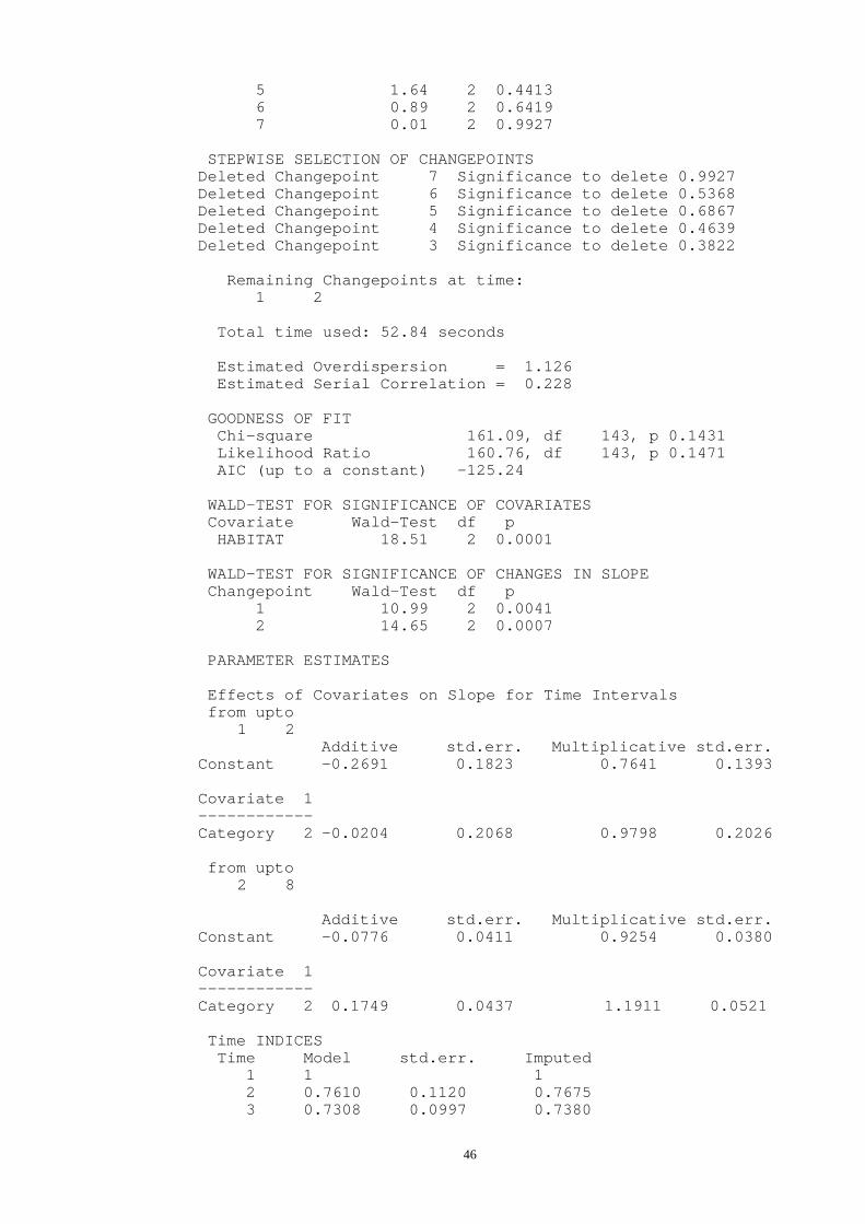
46

5 1.64 2 0.4413 6 0.89 2 0.6419 7 0.01 2 0.9927 STEPWISE SELECTION OF CHANGEPOINTS Deleted Changepoint 7 Significance to delete 0.9927 Deleted Changepoint 6 Significance to delete 0.5368 Deleted Changepoint 5 Significance to delete 0.6867 Deleted Changepoint 4 Significance to delete 0.4639 Deleted Changepoint 3 Significance to delete 0.3822

Remaining Changepoints at time: 1 2

Total time used: 52.84 seconds Estimated Overdispersion = 1.126

Estimated Serial Correlation = 0.228 GOODNESS OF FIT Chi-square 161.09, df 143, p 0.1431 Likelihood Ratio 160.76, df 143, p 0.1471 AIC (up to a constant) -125.24 WALD-TEST FOR SIGNIFICANCE OF COVARIATES Covariate Wald-Test df p HABITAT 18.51 2 0.0001 WALD-TEST FOR SIGNIFICANCE OF CHANGES IN SLOPE Changepoint Wald-Test df p 1 10.99 2 0.0041 2 14.65 2 0.0007 PARAMETER ESTIMATES Effects of Covariates on Slope for Time Intervals from upto


Constant -0.2691 0.1823 0.7641 0.1393 Covariate 1 ------------ Category 2 -0.0204 0.2068 0.9798 0.2026 from upto

2 8

Additive std.err. Multiplicative std.err. Constant -0.0776 0.0411 0.9254 0.0380 Covariate 1 ------------ Category 2 0.1749 0.0437 1.1911 0.0521 Time INDICES Time Model std.err. Imputed 1 1 1

2 0.7610 0.1120 0.7675 3 0.7308 0.0997 0.7380

47

4 0.7056 0.0947 0.6931 5 0.6852 0.0955 0.6461 6 0.6697 0.1000 0.6878 7 0.6590 0.1067 0.6665 8 0.6531 0.1142 0.6571 TIME TOTALS Time Model std.err. Imputed 1 1895.10 263.0260 1900.60 2 1442.17 178.6069 1458.65 3 1384.95 131.3458 1402.55 4 1337.15 97.2911 1317.32 5 1298.61 80.1280 1227.94 6 1269.20 80.9238 1307.25 7 1248.89 93.3720 1266.67 8 1237.70 110.1965 1248.92 OVERALL SLOPE (with intercept) Additive std.err. Multiplicative std.err. -0.0475 0.0249 0.9536 0.0237 OVERALL SLOPE (through base time point) Additive std.err. Multiplicative std.err. -0.0782 0.0295 0.9248 0.0272

Skylark.f1 file

< Site 1 is a Heathland site and site 6 is a Dune site, which is weighted 10 times. Compare these with the fit-ted values of Run 3. > 1, 1, 11 , 8.09 , 11.00, 1, 2, 8 , 6.06 , 8.00, 1, 3, 5 , 6.68 , 5.00, 1, 4, 4 , 7.36 , 4.00, 1, 5, 10 , 8.11 , 10.00, 1, 6, 7 , 8.94 , 7.00, 1, 7, -1 , 9.86 , 9.86, 1, 8, -1 , 10.86 , 10.86, ……

6, 1, 150 , 196.27 , 150.00, 6, 2, 160 , 149.97 , 160.00, 6, 3, 140 , 138.77 , 140.00, 6, 4, 120 , 128.41 , 120.00, 6, 5, 120 , 118.83 , 120.00, 6, 6, 130 , 109.96 , 130.00, 6, 7, 120 , 101.75 , 120.00, 6, 8, 110 , 94.15 , 110.00, etc.

48

5. References

Agresti, A., 1990. Categorical Data Analysis. Wiley, New York.

Amemiya, T, 1985. Advanced Econometrics. Blackwell, London.

Baker, R.J. & J.A. Nelder, 1978. The GLIM System, Release 3. NAG Central Office, London.

Braak, C.J.F. ter, A.J. van Strien, R. Meijer, & T.J. Verstrael, 1994. Analysis of monitoring data with many missing values: which method? In: W. Hagemeijer & T. Verstrael (eds). Bird Numbers 1992. Distribution, Monitoring and Ecological aspects. Proc. 12th Int. Conf. of IBCC and EOAC, 663-673. Statistics Netherlands, Voorburg & Sovon, Beek-Ubbergen.

Fienberg, S.E., 1977. The analysis of cross-classified categorical data. MIT press. Cambridge, Massachusetts.

Liang, K.Y. & S.L. Zeger, 1986. Longitudinal data analysis using generalized linear models. Biometrika, 73, 13-22.

Maddala, G.S., 1977. Econometrics. McGraw-Hill, New York.

McCullagh, P. & J.A. Nelder, 1989. Generalized Linear Models, 2nd edition. Chapman and Hall, London.

Morrison, D.F., 1990. Multivariate Statistical Methods, third edition. McGraw-Hill, New York.

Rao, C.R., 1973. Linear Statistical Inference and Its Applications, 2nd edition. Wiley, New York.

Strien, A.J. van, J. Pannekoek, E.J.M. Hagemeijer & T.J. Verstrael, 1995. A loglinear Poisson regression method to analyse bird monitoring data. Paper presented at: Bird Numbers Conference 1995.

Strien, A.J. van, J. Pannekoek & D.W. Gibbons, in press. Indexing European bird population trends using results of national monitoring schemes: a trial of a new method. Bird Study.

Thomas, L. 1996. Monitoring long-term population change: why are there so many analysis methods? Ecology, 77, 49-58.

Weinreich, J.A. & J.H. Oude Voshaar, 1992. Population trends of bats hibernating in marl caves in the Netherlands (1943-1987). Myotis 30, 75-84.

Zeger, S.L. & K.Y. Liang, 1986. Longitudinal data analysis for discrete and continuous outcomes. Biometrics, 42, 121-130.

49

6. Appendix A. Details of the estimation procedure

6.1 Matrix formulation

To facilitate the discussion of estimators for the model parameters, it is convenient to formulate the models in matrix notation. If we collect the expected frequencies in an IJ-vector µ = ( ,..., ,..., )µ µ µ11 1J IJ , all models can be written as

Ln µµµµ αααα ββββ= +A B , (6.1)

with αααα a pa-vector containing the site-parameters and ββββ a pb-vector containing the time related parameters (this can be β- and/or γ-parameters, depending on the model) and A and B 'design' matrices for the site-effects and time-effects. For all models in TRIM, pa=I and A is an IJ×I-matrix with I dummy-variables, one for each site, and αααα is an I-vector with site-parameters, again one for each site. The matrix Band vector ββββ are specific for each model.

The parameter vectors αααα and ββββ can be combined to one vector θθθθ αααα ββββ= ′ ′ ′( , ) and the

design matrices A and B can be combined to one IJ×p design matrix X=(A,B) with p=pa+pb. The model (6.1) can then be written as

Ln µµµµ θθθθ= X (6.2)

Models for weighted counts can be specified as

Ln diag( )w Xµµµµ θθθθ= (6.3a)

or

Ln Lnµµµµ θθθθ= −X w (6.3b)

with w an IJ-vector containing the cell weights and diag(w) a diagonal matrix with w on the diagonal.

6.2 Generalized estimating equations

The estimation method used in TRIM is based on generalized estimating equations (GEE) see, Liang & Zeger (1986), Zeger & Liang (1986), McCullagh & Nelder, (1989, ch. 9). Contrary to maximum-likelihood (ML) this method doesn’t require the distribution of the observations to be specified in full. The specification (up to some unknown parameters) of the first two moments (expectation and covariance matrix) is sufficient. This makes it relatively easy to take overdispersion and serial correlation into account. Furthermore, the GEE approach to estimating loglinear models reduces to the usual maximum likelihood approach if the covariance matrix of the observations equals the covariance matrix of independent Poisson observa-tions (overdispersion factor is 1 and serial correlation is 0).

For estimating the parameters only the observed counts can be used and therefore, in this section, the vector f refers to the O-vector (O≤IJ) with observed counts only

50

and similarly the rows of the matrices X, A and B corresponding with missing counts are deleted such that the dimensions of these matrices are now O×p, O×pa

and O×pb, respectively.

Given the values of the parameters in the covariance matrix, the GEE estimator $θθθθfor θθθθ is the solution of the estimating equation

U D V f 0( $) ( )θθθθ µµµµ= ′ − =−1 , (6.4)

with D the O×p matrix ∂µµµµ/∂θθθθ and V the covariance matrix of f, the O-vector with observed frequencies (O≤IJ). Since the elements of D are given by D X,ij k ij k ijk ij= =∂µ ∂θ µ we can write D====diag(µ)X and for the estimating function

U(θθθθ) we have

U X V f( ) ( ) ( )θθθθ µµµµ µµµµ= ′ −−diag 1 . (6.5)

If the counts were assumed to be independently Poisson distributed, V would be diag(µ) and the function U(θθθθ) would reduce to X'(f-µ) which is well known to be the score-function (derivative w.r.t. θθθθ) of the likelihood associated with this assump-tion.

The expected value of the derivative matrix ∂∂∂∂ θθθθ ∂∂∂∂θθθθU( ) / ′ is

− ′ = −−D V D i1 ( )θθθθ , (6.6)

where i( )θθθθ plays the same role as the Fisher information matrix for likelihood func-

tions. In particular, if the model is correct and the observed counts are large, the distribution of the GEE estimator $θθθθ is approximately normal with covariance ma-

trix i( )θθθθ −1 .

For given values of the correlation and dispersion parameters, the GEE estimator for θθθθ (the solution of (6.4)) is usually obtained by Fisher scoring iterations given by

θθθθ θθθθ θθθθ θθθθ

θθθθ µµµµt t t t

t t t t t t t

+−

− − −

= +

= + ′ ′ −1

1

1 1 1

i UD V D D V f( ) ( )

( ) ( ) (6.7)

where t is the iteration number and θθθθ µµµµt t t t, ,V D and are estimates at iteration t. If

V=diag(µ) (the Poisson assumption), the current estimate of V would be diag(µ(θθθθt)) and depend on the current estimate of θθθθ only. In our applications we are often not willing to assume that V=diag(µ) because it is likely that overdispersion and serial correlation are present and V will depend on µ as well as on dispersion and correla-tion parameters and estimates of these parameters are required in order to update θθθθ.Consequently, the algorithm iterates between updating θθθθ and estimating the disper-sion and correlation parameters as described in section (6.3).

A problem with the updating equation (6.7) is the size (p×p) of the matrix ′ −D V Dt t t1 .

The number of parameters p is at least equal to the number of sites I, which can be over 1000. Inverting such large matrices is very time and memory consuming. The

51

matrix V is of course even larger (O×O), but for this matrix a block diagonal struc-ture is assumed (section 6.3) which reduces the problem to inverting the covariance matrices for the observations for each site separately. As an alternative to (6.7) an algorithm can be applied that uses the derivatives of U(θθθθ) with respect to ββββ only. This procedure leads to an algorithm that is much faster and less memory consum-ing than an algorithm based on (6.7) and is described in section (6.4).

6.3 Estimation of the covariance matrix

To allow for overdispersion and serial correlation, the O×O covariance matrix V of

f is expressed as σ 2 diag diag( ) ( )µµµµ µµµµ12

12R , with σ 2 a dispersion parameter and R a

correlation matrix, which reduces to diag( )µµµµ if σ 2 =1 and R is the identity matrix.

A simple correlation matrix R that reflects serial correlation is obtained by assum-ing that within each site there is a constant correlation, ρ say, between the observed counts at times j and j-1 and that counts from different sites are uncorrelated. This leads to a block diagonal correlation matrix of the form

R

R

R

R

=

1

O

Oi

I

(6.8)

with Ri the Oi×Oi correlation matrix of the Oi observations in site i. If there are no missing values in a site i then Ri is a J×J matrix and can be expressed as

R i =

− − −

−

−

11

11

2

2 3

1

2ρ

ρ

ρ ρρ

ρ ρ

ρρ

M

L

L

M M

L

MJ J J

J

J

(6.9)

which reflects a declining correlation between counts as they are further apart in time. For sites with missing values the correlation matrix can be obtained from (6.9) by deleting the rows and columns corresponding to the time-points for which there are no observations. Morrison (1990, pag. 381) gives explicit expressions for the elements of the inverse of R i , with or without missing observations.

Following Liang and Zeger (1986), estimates of σ 2 and ρ can be obtained from

the Pearson residuals ( rij , say) as

$σ δ2 21= ∑dfrij ijij

(6.10)

and

52

$$

,ρσ

δ δ=

+=

−

= =

−

=∑∑ ∑∑12 11

11 1

11ij ij i jj

JiI

ijjJ

iIr r (6.11)

where r fij ij ij ij= −( ) /µ µ .

6.4 An efficient algorithm

Using the partitioning θθθθ αααα ββββ= ′ ′ ′( , ) of the parameter vector and the corresponding

partitioning X=(A,B), the estimating equation U(θθθθ)=0 can be expressed in two equations as

U A V fa diag= ′ − =−( ) ( )µµµµ µµµµ1 0 (6.12a)

U B V fb diag= ′ − =−( ) ( )µµµµ µµµµ1 0 (6.12b)

The negative expected derivative matrix i( )θθθθ , defined in (6.6), can be partitioned

similarly leading to

iU UU U

A A A BB A B B

( )θθθθ∂∂∂∂ ∂∂∂∂αααα ∂∂∂∂ ∂∂∂∂ββββ∂∂∂∂ ∂∂∂∂αααα ∂∂∂∂ ∂∂∂∂ββββ

= −′ ′′ ′

=

′ ′′ ′

a a

b b

ΩΩΩΩ ΩΩΩΩΩΩΩΩ ΩΩΩΩ

(6.13)

with ΩΩΩΩ = −diag diag( ) ( )µµµµ µµµµV 1 .

The equations (6.12a, 6.12b) can be solved in two steps. First we solve (6.12a) with respect to αααα using the value for ββββ from the previous iteration and substitute the re-sulting value $ ( )αααα ββββ , say in (6.12b), leading to

U Ub b* ( $ ( ), )= αααα ββββ ββββ . (6.14)

Second, we solve (6.14) with respect to ββββ. With the new value for ββββ the two steps can be repeated. This process can be iterated until convergence. The resulting esti-mates for αααα and ββββ solve the equations (6.12a, 6.12b) and hence U(θθθθ)=0. This two-step procedure is similar to the “concentrated likelihood” approach for solving like-lihood equations (see, Amemiya, 1985, Ch. 4.2.5).

To solve (6.12a) for αααα we note that the matrix A contains dummy variables for each site and the matrix V is a block diagonal covariance matrix of the form (6.8) so that for site i we can write

′ − =−1 V fO i i i iidiag( ) ( )µ µ1 0 (6.15)

with Oi the number of observed counts for site i, 1Oian Oi -vector with ones and fi

the Oi -vector with observed counts for site i with expectation µµµµ i and covariance

matrix Vi . For µµµµ i we can write µµµµ ββββi ia= exp( )Bi , with B i the matrix with the rows

of B corresponding to the observations in site i. Now, (6.15) can be written as

′ − =−µµµµ ββββi i i i iaV f B1 0 $ )exp( (6.16)

leading to

53

$ exp( )ai i i i i i= ′ ′− −µµµµ µµµµ ββββV f V B1 1i and $α i = Lnai$ (6.17)

To solve the equation Ub* = 0 for ββββ a Fisher scoring algorithm analogous to (6.7)

can be used. The expected value of the required derivative matrix, ib* say, can be

written as

( ) ( )− = ′ = ′ + ′ ′i U U Ub b b b* *∂∂∂∂ ∂∂∂∂ββββ ∂∂∂∂ ∂∂∂∂ββββ ∂∂∂∂αααα ∂β∂β∂β∂β ∂∂∂∂ ∂α∂α∂α∂α (6.18)

where the derivatives are evaluated in αααα αααα ββββ= $ ( ) .

Next, differentiating both sides of the equation Ua ( $ ( ), )αααα ββββ ββββ = 0 with respect to ββββ

we obtain

( )( )∂∂∂∂αααα ∂β∂β∂β∂β ∂∂∂∂ ∂α∂α∂α∂α ∂∂∂∂ ∂β∂β∂β∂βαααα αααα′ ′ + ′ =U U 0

and so we have for ∂∂∂∂αααα ∂β∂β∂β∂β′

( )∂∂∂∂αααα ∂β∂β∂β∂β ∂∂∂∂ ∂β∂β∂β∂β ∂∂∂∂ ∂α∂α∂α∂ααααα αααα′ = − ′ ′−U U 1 (6.19)

where again αααα αααα ββββ= $ ( ) . Now, substituting (6.19) in (6.18) and using (6.13) we ob-

tain

( )− = ′ − ′ ′ ′−i B B B A A A A Bb* ΩΩΩΩ ΩΩΩΩ ΩΩΩΩ ΩΩΩΩ

1 (6.20)

The matrices A, B and ΩΩΩΩ can be very large but (6.20) can be rewritten in a form suitable for computation. Since the columns of A are dummy variables indicating the sites and ΩΩΩΩ has the same block diagonal structure as V (and R) we can write

′ =A A dΩΩΩΩ diag( ) , with d the I-vector with elements di o i oi i= ′1 1ΩΩΩΩ and ΩΩΩΩ i the ith

block of ΩΩΩΩ which can be expressed as ΩΩΩΩ i i i idiag diag= −( ) ( )µµµµ µµµµV 1 Now, we can

rewrite (6.20) as

− =ib i* ΣΣΣΣ ′ − ′ ′

B B B A A Bi i i

ii i i i i id

ΩΩΩΩ ΩΩΩΩ ΩΩΩΩ1

= ΣΣΣΣ i ′ − ′

B 1 1 Bi i

ii o o i id i i

ΩΩΩΩ ΩΩΩΩ ΩΩΩΩ1 (6.21)

and so, the matrix − ib* can be build up by a summation of components for each site

that do not involve very large matrices.

In summary, the algorithm alternates between updating αααα and ββββ according to

αit = ′ − ′ −Ln Lni i i i

tz f z Bexp( )ββββ 1

µµµµ αααα ββββt t t Ln= + −−exp( )A B w1 (6.22)

( )ββββ ββββt tb b= −− −1 1

i U* *

and recalculating σ 2 and ρ using the current value of µµµµ .

54

The asymptotic covariance matrix of $ββββ can be estimated by the pb×pb submatrix in

the lower-right corner of − −i( )θθθθ 1 evaluated at θθθθ θθθθ= $ . But, using the formula for the

inverse of a partitioned matrix, it can be seen that this inverse equals the inverse of the right-hand side of (6.20) evaluated at the estimates $ , $αααα ββββ . So, after convergence

of the algorithm (6.22) the matrix ( )−−

ib* 1

provides an estimate of the covariance

matrix of $ββββ .

6.5 Standard errors of model-based time-totals and indices

The J-vector with estimated time-totals can be written as

$ $ ,t C= µ (6.23)

where the J×IJ matrix C can be expressed as C I I I= J J J, , ,K with I J an J by J

identity matrix and the number of identity matrices is equal to the number of sites. The covariance matrix of the estimated time-totals can be expressed as

var($) var( $) var( $)( ) var( $) ( )

t C C CD D CC X X C

= ′ = ′ ′

= ′ ′

µ θµ θ µdiag diag ,

(6.24)

where we have used the usual Taylor-series approximation var( $) var( )µ θ= ′D D

with D = ′∂µ ∂θ .

To compute the standard errors of the model-based time-totals according to (6.24) we need the covariance matrix of the complete parameter vector θθθθ . This matrix is not easy to compute because it requires inversion of a very large matrix, as pointed out in section 6.2. An alternative formula for var($)t that is suitable for computation will be derived in this section.

Consider the partitioned form of (6.13) of i( )θθθθ

iA A A BB A B B

i ii i

( )θ =′ ′′ ′

= ′

Ω ΩΩ Ω

aa ab

ab bb (6.13)

with ΩΩΩΩ = −diag diag( ) ( )µµµµ µµµµV 1 .

The inverse of this partitioned matrix can be expressed as (Rao, 1973, page 33)

i i FE F FEE F E1( )θ −

− − −

− −=+ ′ −− ′

=

11 1 1

111 12

21 22

aa Φ ΦΦ Φ

(6.25)

where

i A A daa diag= ′ =Ω ( ) , E i i i i i= − ′ =−bb ab aa ab

1β*

55

and F i i d A Bw B

w B= = ′ =

′

′

− −

−

−aa ab

I I I

diagd

d

1 11

11 1

1( ) Ω M ,

with w 1 Ri o i ij j i k i jki= ′ =∑ΩΩΩΩ ( ) ( ) ( )µµµµ µµµµ

12

12 and di o ii

= ′1 w .

From this representation we see that we only need the inverse of E (which is already produced by the algorithm) and the inverse of iaa (which is a diagonal matrix) in

order to calculate the inverse of i( )θθθθ .

The covariance matrix of the estimated time-totals can now be expressed as

var($) ( ) var( $) ( )( )[ ] ( )

t C X X CC A A B A A B B B C

= ′ ′′ + ′ + ′ + ′ ′

diag diagdiag diag

µ θ µµ µ

= Φ Φ Φ Φ11 21 12 22

= ′ + ′ + ′ + ′

= ′ + ′ − ′ − ′ + ′− − − − −

G G H G G H H H

G d G GFE GF HE GF GFE H HE H1 1 1

Φ Φ Φ Φ11 21 12 221 1diag( ) ( ) ( )

= ′ + − − ′− −G d G GF H E GF H1diag( ) [ ] [ ] ,1 (6.26)

with G C A= diag( )µ and H C B= diag( )µ .

To compute the covariance matrix (6.26) the following expressions for the elements of the J×I matrix G , the J× pb matrix GF , the J× pb matrix H and the J×J matrix

G d G1diag( )− ′ are used:

( )G ij ji= µ , ( ) ( )GF Fjk iji ik=∑ µ , ( ) ( )H Bjk ii jk ij=∑ µ and

( ( ) )G d Gdiag djk ij iki i− −′ =∑1 1µ µ .

So, the matrices GF-H and G d Gdiag( )− ′1 can be obtained by a summation over

sites.

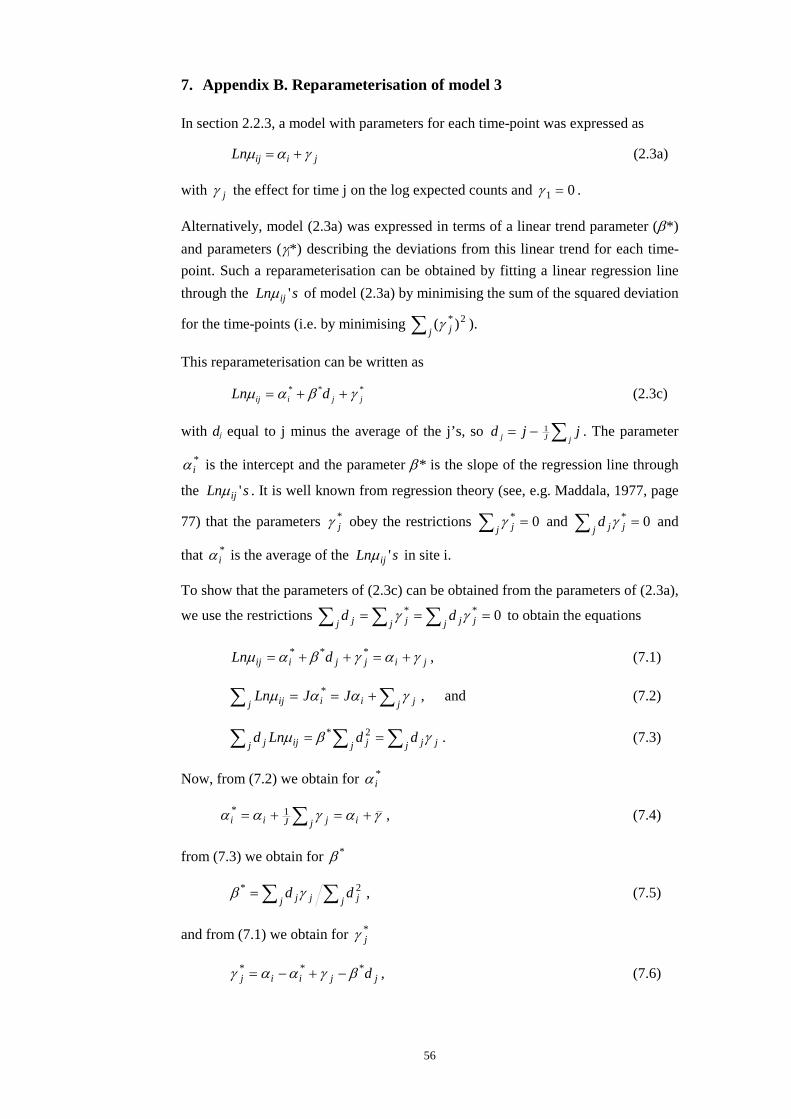
56

7. Appendix B. Reparameterisation of model 3

In section 2.2.3, a model with parameters for each time-point was expressed as

Ln ij i jµ α γ= + (2.3a)

with γ j the effect for time j on the log expected counts and γ 1 0= .

Alternatively, model (2.3a) was expressed in terms of a linear trend parameter (β*) and parameters (γj*) describing the deviations from this linear trend for each time-point. Such a reparameterisation can be obtained by fitting a linear regression line through the Ln sijµ ' of model (2.3a) by minimising the sum of the squared deviation

for the time-points (i.e. by minimising ( )*γ jj∑ 2 ).

This reparameterisation can be written as

Ln dij i j jµ α β γ= + +* * * (2.3c)

with dj equal to j minus the average of the j’s, so d j jj J j= − ∑1 . The parameter

α i* is the intercept and the parameter β* is the slope of the regression line through

the Ln sijµ ' . It is well known from regression theory (see, e.g. Maddala, 1977, page

77) that the parameters γ j* obey the restrictions γ jj

*∑ = 0 and d j jjγ *∑ = 0 and

that α i* is the average of the Ln sijµ ' in site i.

To show that the parameters of (2.3c) can be obtained from the parameters of (2.3a),

we use the restrictions d djj jj jj j∑ ∑ ∑= = =γ γ* * 0 to obtain the equations

Ln dij i j j i jµ α β γ α γ= + + = +* * * , (7.1)

Ln J Jijj i i jjµ α α γ∑ ∑= = +* , and (7.2)

d Ln d dj ijj jj j jjµ β γ∑ ∑ ∑= =* 2 . (7.3)

Now, from (7.2) we obtain for α i*

α α γ α γi i J jj i* = + = +∑1 , (7.4)

from (7.3) we obtain for β *

β γ* =∑ ∑d dj jj jj2 , (7.5)

and from (7.1) we obtain for γ j*

γ α α γ βj i i j jd* * *= − + − , (7.6)

57

8. Appendix C. A procedure to classify trend estimates

Van Strien et al. (in press) have characterised the trends to the following five catego-ries (see table 9). This is not implemented in TRIM.

• the 95% confidence interval of a trend estimate is computed by multiplying the standard error by 1.96. If this interval does not include the value 1, then the trend is statistically significant;

• the lower and upper limit of the confidence interval is converted into the corresponding magnitudes of change in a 20-year period, using the lower and upper limits of the interval as factors. Thus, a lower limit of 0.95 results in a magnitude of change of (0.95)19 in 20 years.

• if the trend is significant and the magnitude of change is significantly greater than 20% in a 20-year period, then the trend was considered as a (1) substantial decline or increase;

• if the trend is significant, yet the change was significantly less than 20%, the trend is classified as a (2) non-substantial decline or increase;

• if the trend is significant, but not significantly different from a 20% change, the trend is classified as a (3) decline or increase;

• if the trend is not significant and the confidence limits were sufficiently small that the trend is significantly less than 20% in a 20-year period, the species is classified as having (4) a stable population;

• if the trend is not significant and the confidence limits are so large that the trend could be larger than 20%, the population trend is classified as (5) “poorly known”, which implies that the statistical power of the scheme for that particular species is too limited to detect a change of less than 20% in 20 years. In such cases, the scheme could still be useful to detect very large changes.

Table 9. Classification of the trend estimates. See text for details.

Greater than 20% change in a 20-year period

Less than 20% change in a 20-year period

Significantly so Not significantly so Not significantly so Significantly so

Significantly different from zero

(1) substantial decline or increase

(3) decline or increase

(3) decline or increase

(2) non-substantial decline or increase

Not significantly different from zero

(impossible)

(5) poorly known

(5) poorly known

(4) stable

trim 3 manual - cbs

Documents