traverse adjustment using excel

8/8/2019 Traverse Adjustment using Excel

http://slidepdf.com/reader/full/traverse-adjustment-using-excel 1/21

Traverse Adjustment Using Microsoft Excel Solver 0/20

Sayed R. Hashimi, Professor

ACSM/TAPS ConferenceApril 19 – 21, 2004, Nashville, TN

Traverse Adjustment Using Microsoft Excel Solver

by:

Sayed R. Hashimi, Professor Surveying Engineering Department

Ferris State University, Big Rapids, MI USA






Traverse Adjustment Using Microsoft Excel Solver by:



Key words: Traverse Adjustment, Least Squares, Excel Solver

Abstract

Simple two-dimensional traverses can easily be adjusted using Compass Rule or Transit Rule.However, when a traverse becomes more complicated with multiple junction points yieldingredundancies greater than three, Compass Rule or Transit Rule adjustments will not be able to doan effective job, particularly when observations (distances and angles) have different weights.Although several least squares adjustment packages are available, Microsoft Excel provides

another option for performing a rigorous least squares traverse adjustment. This paper provides:a brief overview of Excel’s Add-in Solver; basic theory of least squares as implemented withinthe Solver; advantages and disadvantages of the Excel Solver in least squares, and two numericalexamples outlining the steps involved in carrying out a traverse adjustment. The reasons the useof Excel for traverse adjustment can be considered a viable option are: a. Excel is readilyavailable in any Windows platform without any additional cost. b. Excel is easy to use. c. Thedata transfer to and from Excel is very flexible. The paper also provides some useful VisualBasic functions used in traverse adjustment.






Traverse Adjustment Using Microsoft Excel Solver by:



1. INTRODUCTIONSolver is an Add-in tool in Microsoft Excel designed to perform optimization solutions for modeling systems. This paper describes various techniques for modeling survey traverse data to be adjusted by least squares. The models include a single traverse loop and interconnectedtraverse loops where observations are independently weighted.

1.1 About Microsoft Excel SolverThe Excel Solver Engine, developed by Frontline Systems, Inc., is a standard feature of anyMicrosoft Office product. Since the solution of least squares problems requires minimization,Excel with its strong Graphic User Interface (GUI) provides a convenient and readily available

tool, the Solver, to adjust small to medium size traverses encountered in day to day surveying practices. Furthermore, the user does not need to know (1) how to form the condition equations(2) how to differentiate complex equations (3) how to solve the normal equations used in aconventional least squares approach.Solving an optimization model using Excel Solver requires:

• Identifying model resource data

• Specifying the constraints for the model

• Specifying the model objectiveThe above three steps are carried out through the Solver’s GUI dialog box.

In addition to the standard Solver, Frontline Systems provides Premium Solver Platforms tohandle very large optimization models including a DLL Platform which can interface withVisual Basic and C/C++ programming languages. For additional information the reader isencouraged to visit the Frontline web site at http://www.frontsys.com. The site contains links tothe most current information on the Solver platforms, examples, tutorials on differentoptimization models, although not much on least squares application to surveying problems. Itshould be pointed out that other spreadsheets such as Lotus 1-2-3 and Quattro Pro also provide asimilar optimization model also developed by Frontline Systems, Inc.

1.1.1 Microsoft Excel Solver InstallationAs stated earlier, Solver is an Excel Add-in tool available from TOOLS/SOLVER … If the Solver is not available, then it could be due to: (1) Solver is installed but not selected or (2) Solver is notinstalled.

1.1.1.1 Solver is installed but not selectedIf Solver is installed, then from the TOOLS menu select ADD-INS… This will display all theavailable ADD-INS as shown in Figure 1.






Figure 1Check Solver Add-in box and click OK .

1.1.1.2 Solver is not installedIf Solver is not installed, then the Solver Add-in option in Figure 1 will not be available. In thiscase, use Microsoft Office CD and install the Excel Add-in. The Microsoft Excel online help and

the Microsoft Office Web site provide excellent sources of reference to review when needed.

1.2 Adaptation of Traverse to Excel Solver

While it is not necessary for the user to understand the theory of traverse adjustment by leastsquares, it is however, important to understand the basic geometry of positioning. The geometricdefinition of the functional model described by Mikhail (1976) represents the mathematicalrelationships between points and lines. To aid in this analysis the following variables are defined:

• no is the minimum number of observations needed to fix the model uniquely. Obviously,there must be some redundant observations in the model in order for any adjustment to take

place.• n is the total number of observations in the model.

• r is the total number of redundancies in the model, total number of observations minus theminimum number of observations needed to fix the model uniquely (r = n – no). Typically,in a close traverse where all the distances and angles are measured, there are threeredundancies.

• w is the observation weight, and it is calculated as the inverse of the standard deviationsquared. For angular observations, the standard deviation must be expressed in radians.

• v is the residual which is equal to the adjusted observation minus the observation( observed Adjusted v −= ).

1.2.1 Least Squares PrincipleThe optimized solution in least squares is to minimize the weighted sum of the squares of the residuals

( MinimumvW ii→⋅∑ 2

). In a two-dimensional traverse, the observations consist of distances, and

horizontal angles. The adjusted distances and adjusted angles are computed as functions of latitudes






(distance X Cos(observed azimuth) and departures (distance X Sin(observed azimuth)). The observedazimuth is:

32121.12. Angle Az Az +±−=− π (1)

Where Az.1 - 2, and Az. 2 - 3 are the respective azimuths from 1 to 2 and2 to 3 derived from the observations.

The adjusted distances and adjusted angles are calculated as follows:

22. Departure Latitude Dist Adj += (2)

Figure 2

(3)

Note that equation (3) is specific to Figure 1 where line 1 2 is in quadrant 1, and line 2 3 is in quadrant 2.Similar provisions must be made for lines in other quadrants.

Equations (1), (2) and (3) are the principle equations the user needs to know. Furthermore, the Appendixcontains a collection of user-defined Visual Basic (VB) functions that can be used to further simplify the process, for example, the function azrad(x1, y1, x2, y2) can be used to calculate the azimuth in radiansfrom point 1 to point 2.

1.2.2 Design of a Traverse Model

Identifying model resource data: The traverse resource data are observations (angles,distances), fixed coordinates and fixed azimuths. Observed azimuths are calculated from angleobservations using equation (1). A traverse must have a minimum of one point fixed (knowncoordinates) and one fixed azimuth in order to carryout any adjustment. Latitudes and departuresare calculated using the observed distances and the observed azimuths. Using the computedlatitudes and departures, adjusted distances and angles are calculated using equations (2) and (3).

The observation standard deviations are used to compute the associated weights as 2/1 σ =w ,

where σ is the standard deviation. The standard deviation of angles must be expressed in

radians.

Specifying the constraints for the model: In traverse adjustment, the constraints are:• Sum of the latitudes = 0

• Sum of the departures = 0

• Sum of the interior angles = (n-2)*180o for a geometrically closed traverse, where n is thenumber of sides in the traverse. If the traverse originates from a fixed azimuth and closes to

−+

=

−

−

−

−

12

12

32

32 tantan. Lat

Dep Arc

Lat

Dep Arc Angle Adj π






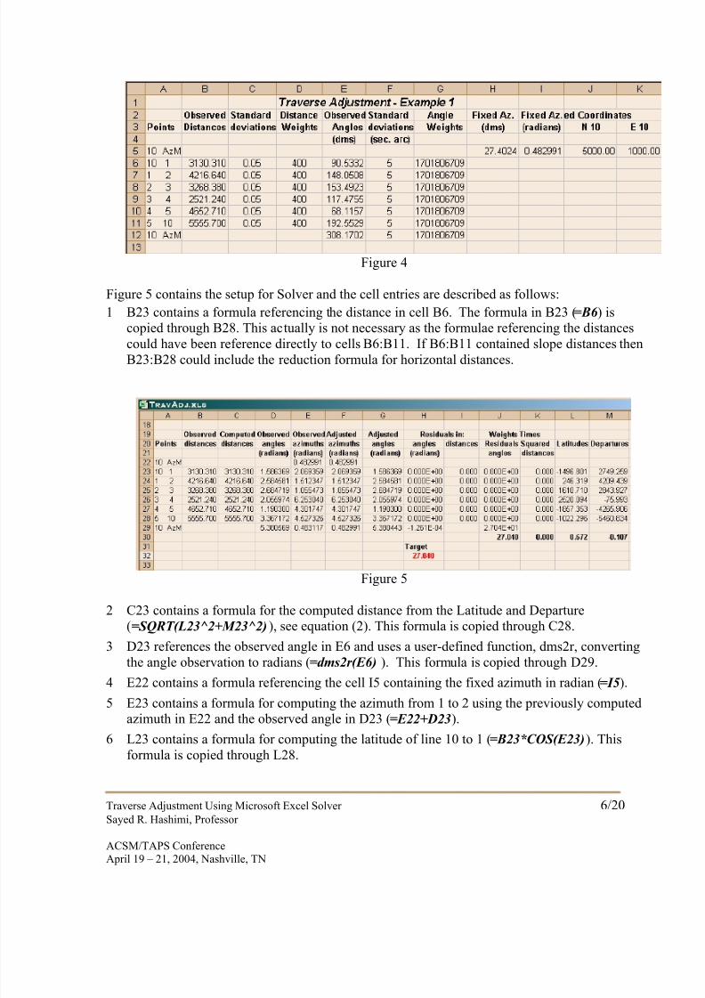
Figure 4

Figure 5 contains the setup for Solver and the cell entries are described as follows:

1 B23 contains a formula referencing the distance in cell B6. The formula in B23 (=B6 ) iscopied through B28. This actually is not necessary as the formulae referencing the distances

could have been reference directly to cells B6:B11. If B6:B11 contained slope distances thenB23:B28 could include the reduction formula for horizontal distances.

Figure 5

2 C23 contains a formula for the computed distance from the Latitude and Departure(=SQRT(L23^2+M23^2)), see equation (2). This formula is copied through C28.

3 D23 references the observed angle in E6 and uses a user-defined function, dms2r, convertingthe angle observation to radians (=dms2r(E6) ). This formula is copied through D29.

4 E22 contains a formula referencing the cell I5 containing the fixed azimuth in radian (=I5).

5 E23 contains a formula for computing the azimuth from 1 to 2 using the previously computedazimuth in E22 and the observed angle in D23 (=E22+D23).

6 L23 contains a formula for computing the latitude of line 10 to 1 (=B23*COS(E23)). Thisformula is copied through L28.






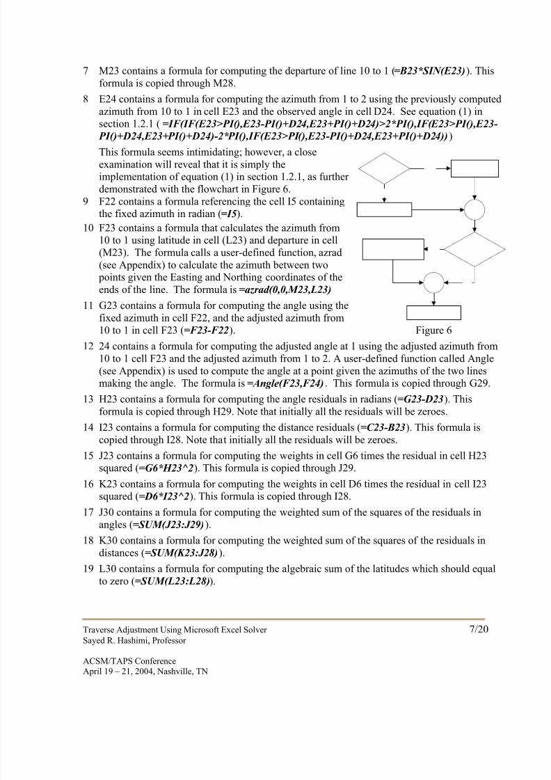
7 M23 contains a formula for computing the departure of line 10 to 1 (=B23*SIN(E23)). Thisformula is copied through M28.

8 E24 contains a formula for computing the azimuth from 1 to 2 using the previously computedazimuth from 10 to 1 in cell E23 and the observed angle in cell D24. See equation (1) insection 1.2.1 ( =IF(IF(E23>PI(),E23-PI()+D24,E23+PI()+D24)>2*PI(),IF(E23>PI(),E23-

PI()+D24,E23+PI()+D24)-2*PI(),IF(E23>PI(),E23-PI()+D24,E23+PI()+D24)))This formula seems intimidating; however, a closeexamination will reveal that it is simply theimplementation of equation (1) in section 1.2.1, as further demonstrated with the flowchart in Figure 6.

9 F22 contains a formula referencing the cell I5 containingthe fixed azimuth in radian (=I5).

10 F23 contains a formula that calculates the azimuth from10 to 1 using latitude in cell (L23) and departure in cell(M23). The formula calls a user-defined function, azrad(see Appendix) to calculate the azimuth between two

points given the Easting and Northing coordinates of theends of the line. The formula is =azrad(0,0,M23,L23)

11 G23 contains a formula for computing the angle using thefixed azimuth in cell F22, and the adjusted azimuth from10 to 1 in cell F23 (=F23-F22). Figure 6

12 24 contains a formula for computing the adjusted angle at 1 using the adjusted azimuth from10 to 1 cell F23 and the adjusted azimuth from 1 to 2. A user-defined function called Angle(see Appendix) is used to compute the angle at a point given the azimuths of the two linesmaking the angle. The formula is =Angle(F23,F24). This formula is copied through G29.

13 H23 contains a formula for computing the angle residuals in radians (=G23-D23). This

formula is copied through H29. Note that initially all the residuals will be zeroes.

14 I23 contains a formula for computing the distance residuals (=C23-B23). This formula iscopied through I28. Note that initially all the residuals will be zeroes.

15 J23 contains a formula for computing the weights in cell G6 times the residual in cell H23squared (=G6*H23^2). This formula is copied through J29.

16 K23 contains a formula for computing the weights in cell D6 times the residual in cell I23squared (=D6*I23^2). This formula is copied through I28.

17 J30 contains a formula for computing the weighted sum of the squares of the residuals inangles (=SUM(J23:J29)).

18 K30 contains a formula for computing the weighted sum of the squares of the residuals indistances (=SUM(K23:J28)).

19 L30 contains a formula for computing the algebraic sum of the latitudes which should equalto zero (=SUM(L23:L28)).






20 M30 contains a formula for computing the algebraic sum of the departures which shouldequal to zero (=SUM(M23:M28)).

21 H32 is the target cell. This in Excel Solver is a single cell whose value will beminimized, maximized, or set equal to a certain value when the Solver finds a solution.In a least squares application it the cell that contains the weighted sums of the squares of

the residuals that must be minimized. The formula in the target cell is =SUM(J30,K30).

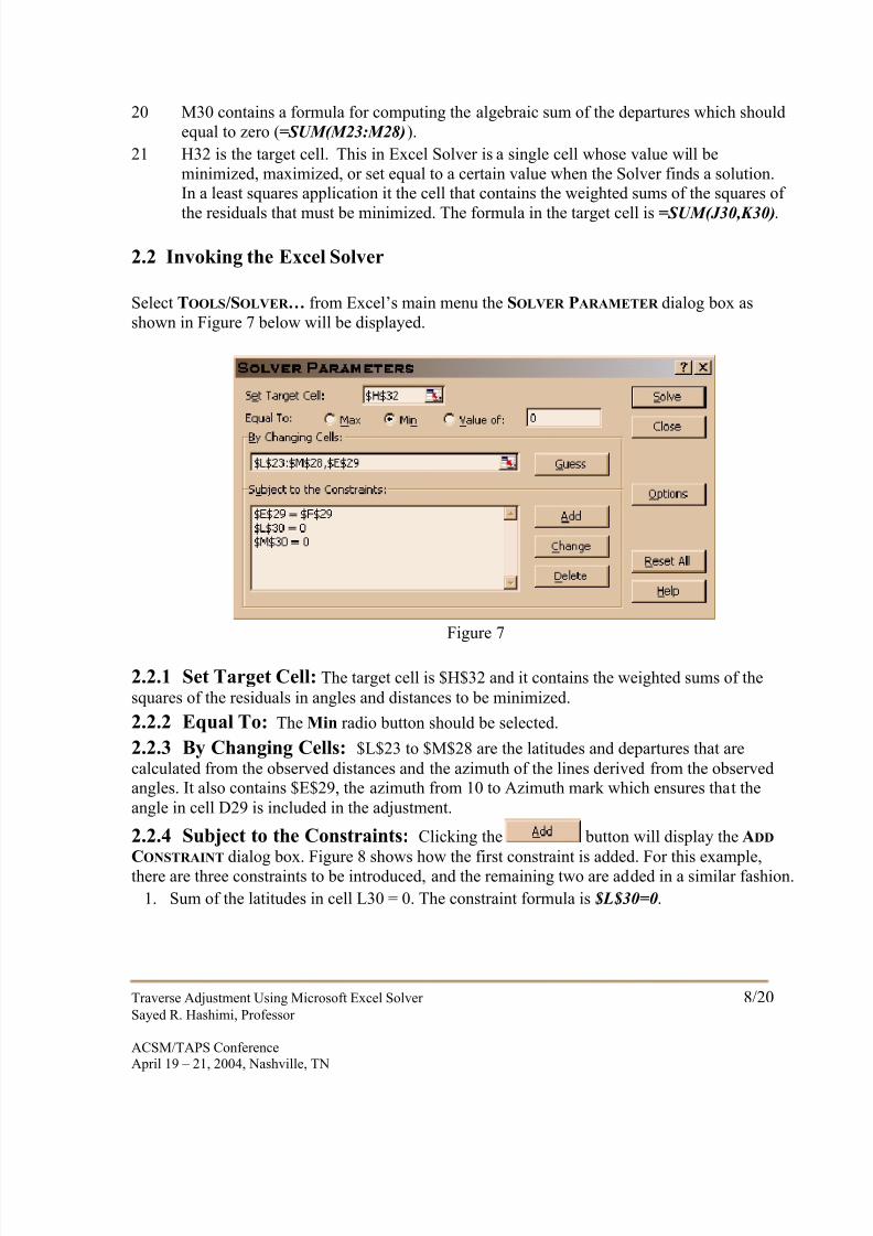
2.2 Invoking the Excel Solver

Select TOOLS/SOLVER … from Excel’s main menu the SOLVER PARAMETER dialog box asshown in Figure 7 below will be displayed.

Figure 7

2.2.1 Set Target Cell: The target cell is $H$32 and it contains the weighted sums of the

squares of the residuals in angles and distances to be minimized.

2.2.2 Equal To: The Min radio button should be selected.

2.2.3 By Changing Cells: $L$23 to $M$28 are the latitudes and departures that are

calculated from the observed distances and the azimuth of the lines derived from the observedangles. It also contains $E$29, the azimuth from 10 to Azimuth mark which ensures that theangle in cell D29 is included in the adjustment.

2.2.4 Subject to the Constraints: Clicking the button will display the ADD

CONSTRAINT dialog box. Figure 8 shows how the first constraint is added. For this example,there are three constraints to be introduced, and the remaining two are added in a similar fashion.

1. Sum of the latitudes in cell L30 = 0. The constraint formula is $L$30=0.






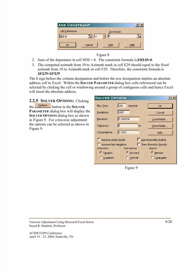
Figure 8

2. Sum of the departures in cell M30 = 0. The constraint formula is $M$30=0.

3. The computed azimuth from 10 to Azimuth mark in cell E29 should equal to the fixedazimuth from 10 to Azimuth mark in cell F29. Therefore, the constraint formula is$E$29=$F$29

The $ sign before the column designation and before the row designation implies an absoluteaddress cell in Excel. Within the SOLVER PARAMETER dialog box cells referenced can beselected by clicking the cell or windowing around a group of contiguous cells and hence Excelwill insert the absolute address.

2.2.5 SOLVER OPTIONS: Clicking

the button in the SOLVER PARAMETER dialog box will display theSOLVER OPTIONS dialog box as shownin Figure 9. For a traverse adjustmentthe options can be selected as shown inFigure 9.

Figure 9






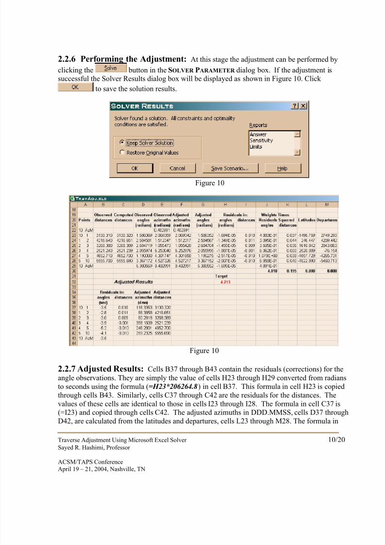
2.2.6 Performing the Adjustment: At this stage the adjustment can be performed by

clicking the button in the SOLVER PARAMETER dialog box. If the adjustment issuccessful the Solver Results dialog box will be displayed as shown in Figure 10. Click

to save the solution results.

Figure 10

Figure 10

2.2.7 Adjusted Results: Cells B37 through B43 contain the residuals (corrections) for theangle observations. They are simply the value of cells H23 through H29 converted from radiansto seconds using the formula (=H23*206264.8) in cell B37. This formula in cell H23 is copiedthrough cells B43. Similarly, cells C37 through C42 are the residuals for the distances. Thevalues of these cells are identical to those in cells I23 through I28. The formula in cell C37 is(=I23) and copied through cells C42. The adjusted azimuths in DDD.MMSS, cells D37 throughD42, are calculated from the latitudes and departures, cells L23 through M28. The formula in






D37 is(=azdms(0,0,M23,L23), and copied through H42. It uses the user-defined azdms function provided in the Appendix of this paper. Adjusted distances, cells E37 through E42 are identicalto cells C23 through C29.

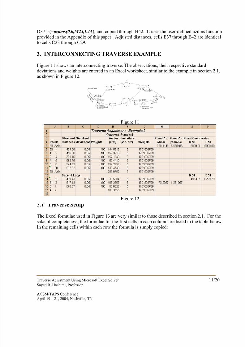
3. INTERCONNECTING TRAVERSE EXAMPLE

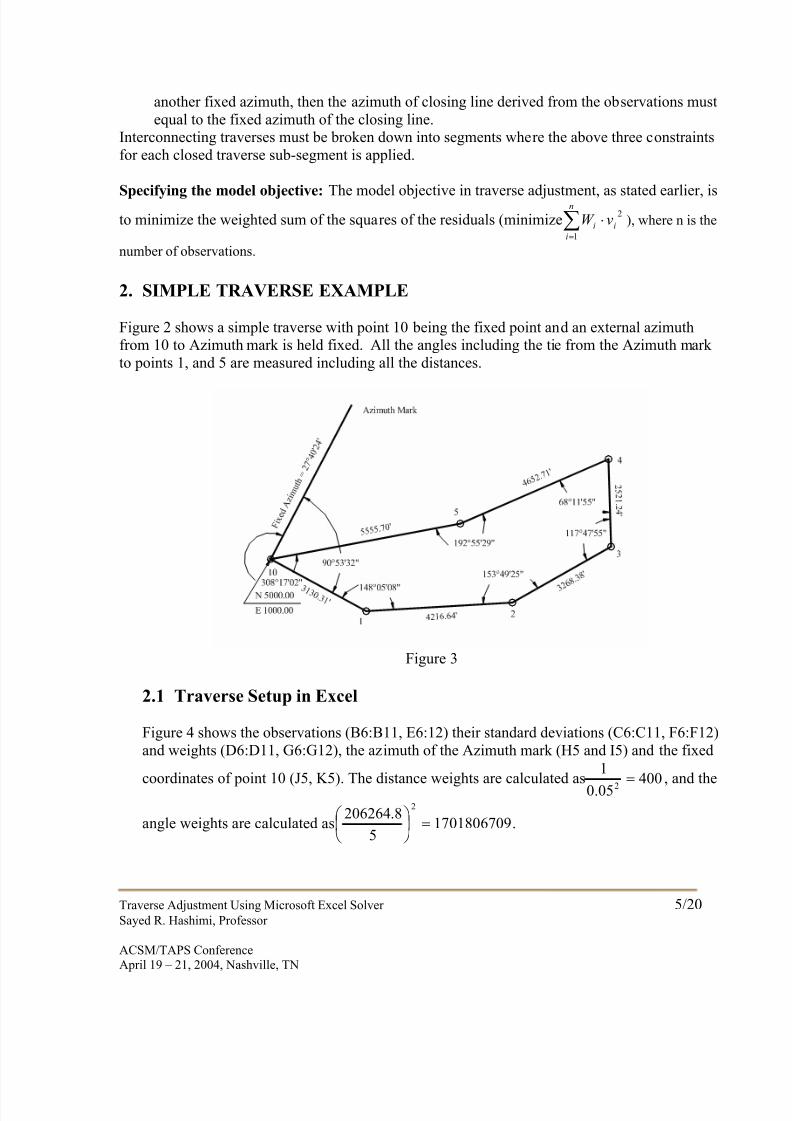
Figure 11 shows an interconnecting traverse. The observations, their respective standarddeviations and weights are entered in an Excel worksheet, similar to the example in section 2.1,as shown in Figure 12.

Figure 11

Figure 12

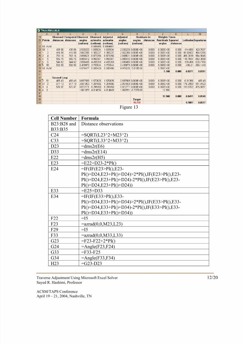
3.1 Traverse Setup

The Excel formulae used in Figure 13 are very similar to those described in section 2.1. For thesake of completeness, the formulae for the first cells in each column are listed in the table below.In the remaining cells within each row the formula is simply copied:

139°47'40"

154°29'52"50°44'10"

163°23'57"192°32'16"

74°52'8"

39°58'4"

1

251

3

4

5

6

Azimuth mark

50

N 5000.00

E 5000.00Fixed N 4973.59

E 6299.79Fixed

106°37'55"

50°00'22"

152°32'16"

144°58'18"

469.43

320 ° 1 1'48 " F ix e d

A z im

ut h 73°23'57"

Fixed

Azi






Figure 13

Cell Number FormulaB23:B28 andB33:B35

Distance observations

C24 =SQRT(L23^2+M23^2)

C33 =SQRT(L33^2+M33^2)

D23 =dms2r(E6)

D33 =dms2r(E14)

E22 =dms2r(H5)

E23 =E22+D23-2*PI()

E24 =IF(IF(E23>PI(),E23-PI()+D24,E23+PI()+D24)>2*PI(),IF(E23>PI(),E23-

PI()+D24,E23+PI()+D24)-2*PI(),IF(E23>PI(),E23-PI()+D24,E23+PI()+D24))

E33 =E25+D33

E34 =IF(IF(E33>PI(),E33-PI()+D34,E33+PI()+D34)>2*PI(),IF(E33>PI(),E33-PI()+D34,E33+PI()+D34)-2*PI(),IF(E33>PI(),E33-PI()+D34,E33+PI()+D34))

F22 =I5

F23 =azrad(0,0,M23,L23)

F29 =I5

F33 =azrad(0,0,M33,L33)

G23 =F23-F22+2*PI()G24 =Angle(F23,F24)

G33 =F33-F25

G34 =Angle(F33,F34)

H23 =G23-D23






H33 =G33-D33

I23 =C23-B23

I33 =C33-B33

J23 =G6*H23^2

J30 =SUM(J23:J29)

J33 =G14*H33^2J38 =SUM(J33:J36)

K23 =D6*I23^2

K30 =SUM(K23:K28)

K33 =D14*I33^2

K38 =SUM(K33:K35)

L23 =B23*COS(E23)

L30 =SUM(L23:L28)

L33 =B33*COS(E33)

L38 =SUM(L33:L35)-L25

L40 =J5+SUM(L23:L24,L33)-J14

M23 =B23*SIN(E23)M30 =SUM(M23:M28)

M33 =B33*SIN(E33)

M38 =SUM(M33:M35)-M25

M40 =K5+SUM(M23:M24,M33)-K14

H40 =SUM(J30,K30,J38,K38)

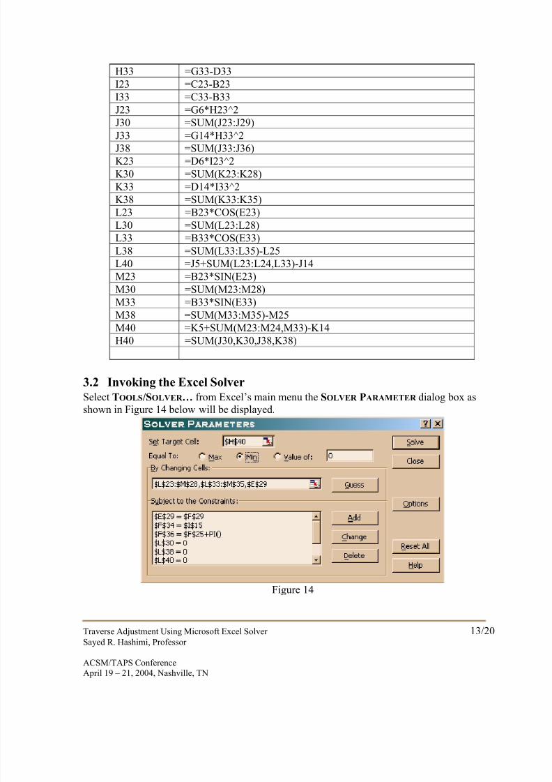
3.2 Invoking the Excel Solver

Select TOOLS/SOLVER … from Excel’s main menu the SOLVER PARAMETER dialog box as

shown in Figure 14 below will be displayed.

Figure 14






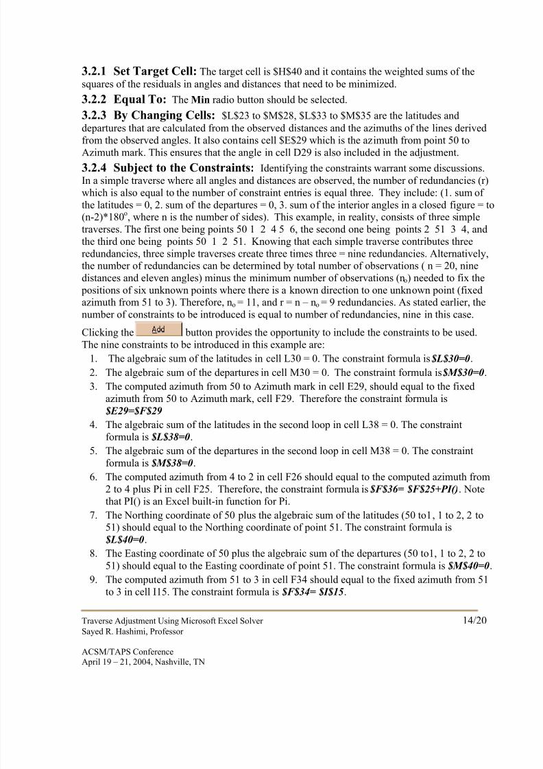
3.2.1 Set Target Cell: The target cell is $H$40 and it contains the weighted sums of the

squares of the residuals in angles and distances that need to be minimized.

3.2.2 Equal To: The Min radio button should be selected.

3.2.3 By Changing Cells: $L$23 to $M$28, $L$33 to $M$35 are the latitudes and

departures that are calculated from the observed distances and the azimuths of the lines derivedfrom the observed angles. It also contains cell $E$29 which is the azimuth from point 50 toAzimuth mark. This ensures that the angle in cell D29 is also included in the adjustment.

3.2.4 Subject to the Constraints: Identifying the constraints warrant some discussions.In a simple traverse where all angles and distances are observed, the number of redundancies (r)which is also equal to the number of constraint entries is equal three. They include: (1. sum of the latitudes = 0, 2. sum of the departures = 0, 3. sum of the interior angles in a closed figure = to(n-2)*180o, where n is the number of sides). This example, in reality, consists of three simpletraverses. The first one being points 50 1 2 4 5 6, the second one being points 2 51 3 4, andthe third one being points 50 1 2 51. Knowing that each simple traverse contributes threeredundancies, three simple traverses create three times three = nine redundancies. Alternatively,

the number of redundancies can be determined by total number of observations ( n = 20, ninedistances and eleven angles) minus the minimum number of observations (no) needed to fix the positions of six unknown points where there is a known direction to one unknown point (fixedazimuth from 51 to 3). Therefore, no = 11, and r = n – no = 9 redundancies. As stated earlier, thenumber of constraints to be introduced is equal to number of redundancies, nine in this case.

Clicking the button provides the opportunity to include the constraints to be used.The nine constraints to be introduced in this example are:

1. The algebraic sum of the latitudes in cell L30 = 0. The constraint formula is $L$30=0.

2. The algebraic sum of the departures in cell M30 = 0. The constraint formula is $M$30=0.

3. The computed azimuth from 50 to Azimuth mark in cell E29, should equal to the fixedazimuth from 50 to Azimuth mark, cell F29. Therefore the constraint formula is$E29=$F$29

4. The algebraic sum of the latitudes in the second loop in cell L38 = 0. The constraintformula is $L$38=0.

5. The algebraic sum of the departures in the second loop in cell M38 = 0. The constraintformula is $M$38=0.

6. The computed azimuth from 4 to 2 in cell F26 should equal to the computed azimuth from2 to 4 plus Pi in cell F25. Therefore, the constraint formula is $F$36= $F$25+PI(). Notethat PI() is an Excel built-in function for Pi.

7. The Northing coordinate of 50 plus the algebraic sum of the latitudes (50 to1, 1 to 2, 2 to51) should equal to the Northing coordinate of point 51. The constraint formula is

$L$40=0. 8. The Easting coordinate of 50 plus the algebraic sum of the departures (50 to1, 1 to 2, 2 to

51) should equal to the Easting coordinate of point 51. The constraint formula is $M$40=0.

9. The computed azimuth from 51 to 3 in cell F34 should equal to the fixed azimuth from 51to 3 in cell I15. The constraint formula is $F$34= $I$15.






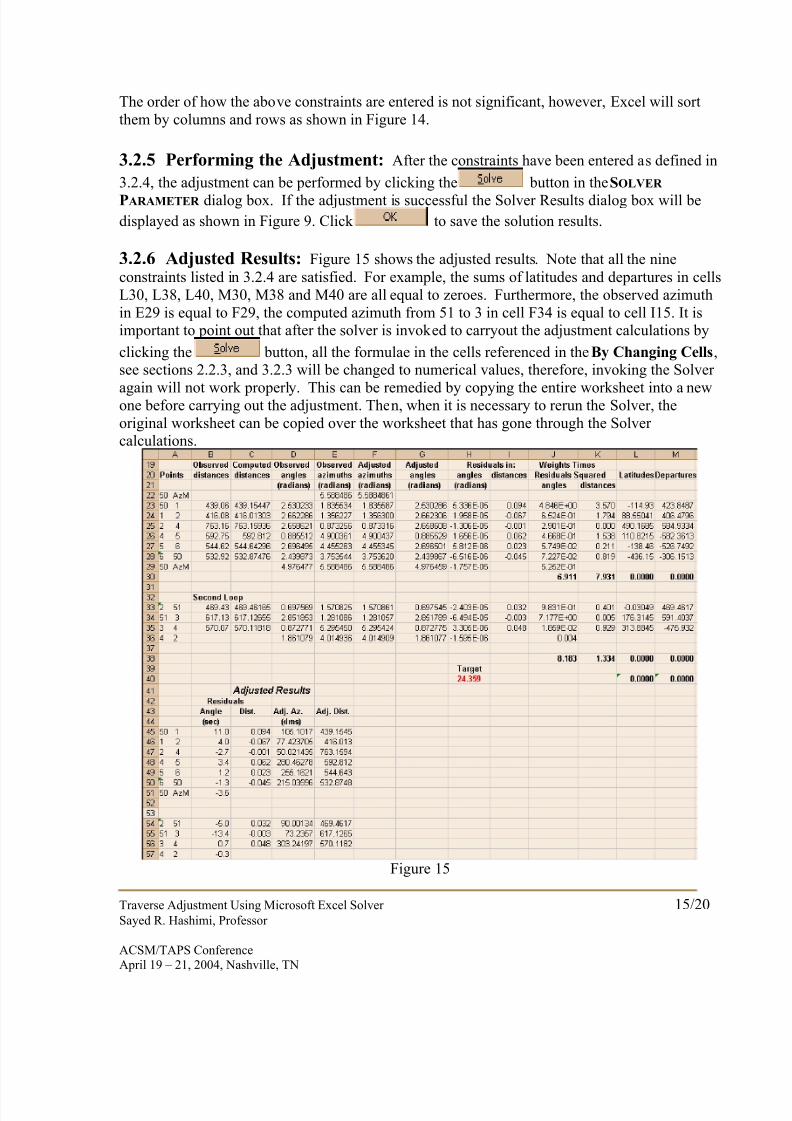
The order of how the above constraints are entered is not significant, however, Excel will sortthem by columns and rows as shown in Figure 14.

3.2.5 Performing the Adjustment: After the constraints have been entered as defined in

3.2.4, the adjustment can be performed by clicking the button in the SOLVER

PARAMETER dialog box. If the adjustment is successful the Solver Results dialog box will be

displayed as shown in Figure 9. Click to save the solution results.

3.2.6 Adjusted Results: Figure 15 shows the adjusted results. Note that all the nineconstraints listed in 3.2.4 are satisfied. For example, the sums of latitudes and departures in cellsL30, L38, L40, M30, M38 and M40 are all equal to zeroes. Furthermore, the observed azimuthin E29 is equal to F29, the computed azimuth from 51 to 3 in cell F34 is equal to cell I15. It isimportant to point out that after the solver is invoked to carryout the adjustment calculations by

clicking the button, all the formulae in the cells referenced in the By Changing Cells,see sections 2.2.3, and 3.2.3 will be changed to numerical values, therefore, invoking the Solver

again will not work properly. This can be remedied by copying the entire worksheet into a newone before carrying out the adjustment. Then, when it is necessary to rerun the Solver, theoriginal worksheet can be copied over the worksheet that has gone through the Solver calculations.

Figure 15






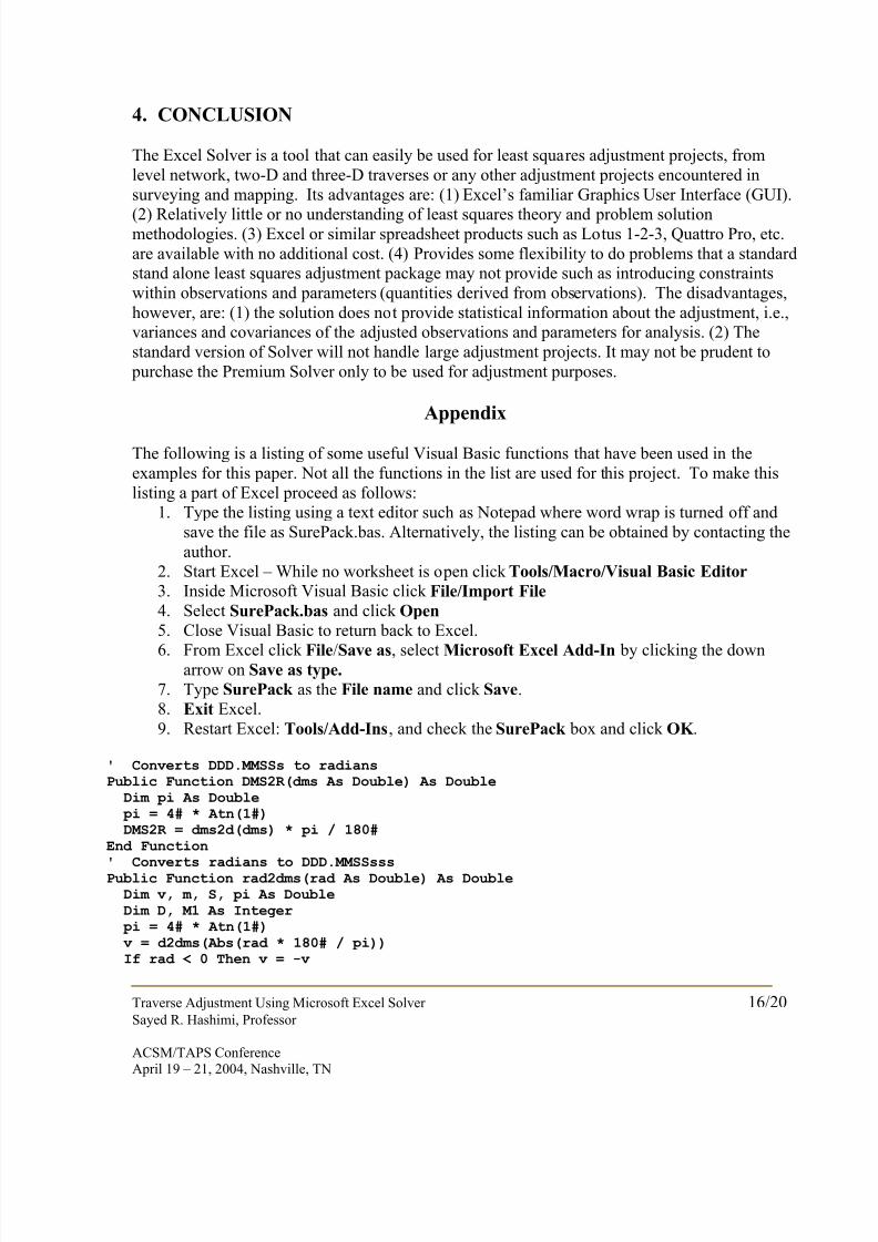
4. CONCLUSION

The Excel Solver is a tool that can easily be used for least squares adjustment projects, fromlevel network, two-D and three-D traverses or any other adjustment projects encountered insurveying and mapping. Its advantages are: (1) Excel’s familiar Graphics User Interface (GUI).

(2) Relatively little or no understanding of least squares theory and problem solutionmethodologies. (3) Excel or similar spreadsheet products such as Lotus 1-2-3, Quattro Pro, etc.are available with no additional cost. (4) Provides some flexibility to do problems that a standardstand alone least squares adjustment package may not provide such as introducing constraintswithin observations and parameters (quantities derived from observations). The disadvantages,however, are: (1) the solution does not provide statistical information about the adjustment, i.e.,variances and covariances of the adjusted observations and parameters for analysis. (2) Thestandard version of Solver will not handle large adjustment projects. It may not be prudent to purchase the Premium Solver only to be used for adjustment purposes.

Appendix

The following is a listing of some useful Visual Basic functions that have been used in theexamples for this paper. Not all the functions in the list are used for this project. To make thislisting a part of Excel proceed as follows:

1. Type the listing using a text editor such as Notepad where word wrap is turned off andsave the file as SurePack.bas. Alternatively, the listing can be obtained by contacting theauthor.

2. Start Excel – While no worksheet is open click Tools/Macro/Visual Basic Editor 3. Inside Microsoft Visual Basic click File/Import File 4. Select SurePack.bas and click Open 5. Close Visual Basic to return back to Excel.

6. From Excel click File/Save as, select Microsoft Excel Add-In by clicking the downarrow on Save as type.

7. Type SurePack as the File name and click Save.8. Exit Excel.9. Restart Excel: Tools/Add-Ins, and check the SurePack box and click OK .

' Converts DDD.MMSSs to radiansPublic Function DMS2R(dms As Double) As DoubleDim pi As Double

pi = 4# * Atn(1#)DMS2R = dms2d(dms) * pi / 180#

End Function' Converts radians to DDD.MMSSsssPublic Function rad2dms(rad As Double) As DoubleDim v, m, S, pi As DoubleDim D, M1 As Integer

pi = 4# * Atn(1#) v = d2dms(Abs(rad * 180# / pi))If rad < 0 Then v = -v






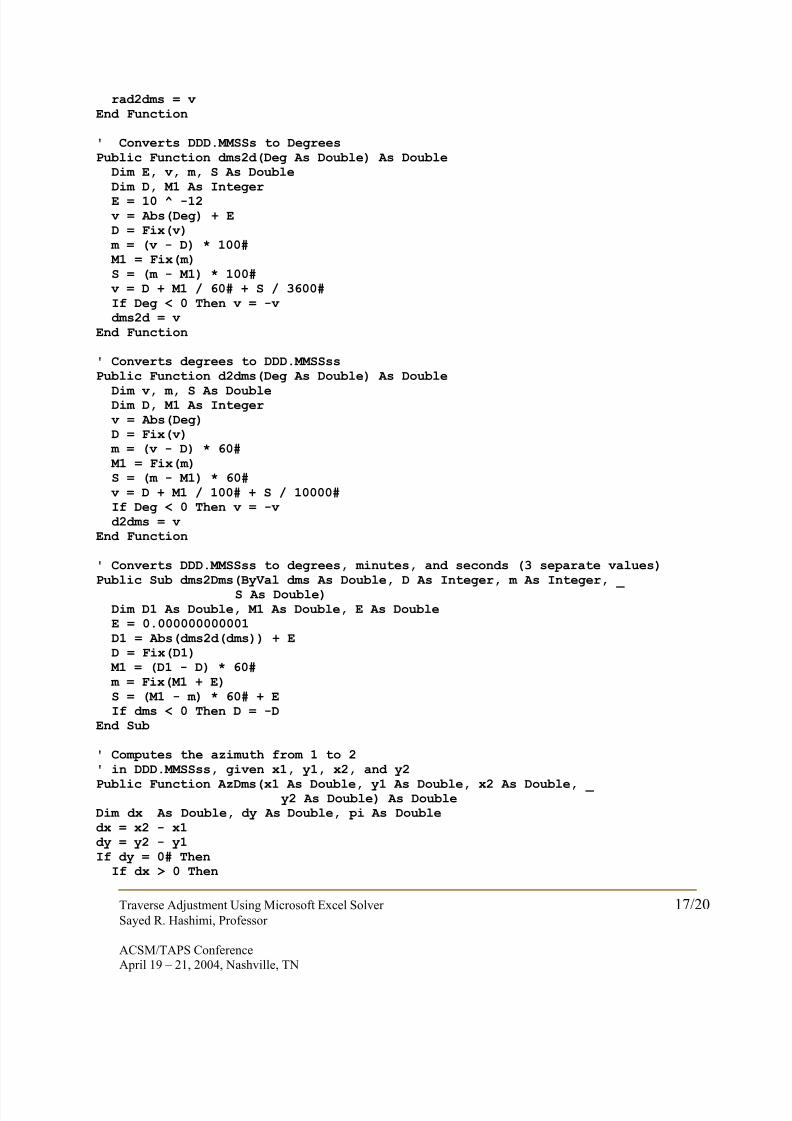
rad2dms = v End Function

' Converts DDD.MMSSs to DegreesPublic Function dms2d(Deg As Double) As DoubleDim E, v, m, S As DoubleDim D, M1 As IntegerE = 10 ^ -12

v = Abs(Deg) + ED = Fix(v)

m = (v - D) * 100# M1 = Fix(m)S = (m - M1) * 100#

v = D + M1 / 60# + S / 3600#If Deg < 0 Then v = -v dms2d = v

End Function

' Converts degrees to DDD.MMSSssPublic Function d2dms(Deg As Double) As Double

Dim v, m, S As DoubleDim D, M1 As Integer

v = Abs(Deg)D = Fix(v)

m = (v - D) * 60# M1 = Fix(m)S = (m - M1) * 60#

v = D + M1 / 100# + S / 10000#If Deg < 0 Then v = -v d2dms = v

End Function

' Converts DDD.MMSSss to degrees, minutes, and seconds (3 separate values)Public Sub dms2Dms(ByVal dms As Double, D As Integer, m As Integer, _

S As Double)Dim D1 As Double, M1 As Double, E As DoubleE = 0.000000000001D1 = Abs(dms2d(dms)) + ED = Fix(D1)

M1 = (D1 - D) * 60# m = Fix(M1 + E)S = (M1 - m) * 60# + EIf dms < 0 Then D = -D

End Sub

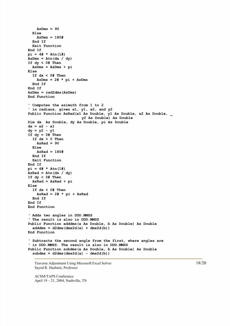
' Computes the azimuth from 1 to 2' in DDD.MMSSss, given x1, y1, x2, and y2

Public Function AzDms(x1 As Double, y1 As Double, x2 As Double, _ y2 As Double) As Double

Dim dx As Double, dy As Double, pi As Doubledx = x2 - x1dy = y2 - y1If dy = 0# ThenIf dx > 0 Then






AzDms = 90Else AzDms = 180#End IfExit Function

End If pi = 4# * Atn(1#) AzDms = Atn(dx / dy)If dy < 0# Then AzDms = AzDms + piElseIf dx < 0# Then AzDms = 2# * pi + AzDmsEnd If

End If AzDms = rad2dms(AzDms)End Function

' Computes the azimuth from 1 to 2' in radians, given x1, y1, x2, and y2

Public Function AzRad(x1 As Double, y1 As Double, x2 As Double, _ y2 As Double) As Double

Dim dx As Double, dy As Double, pi As Doubledx = x2 - x1dy = y2 - y1If dy = 0# ThenIf dx > 0 Then AzRad = 90Else AzRad = 180#End IfExit Function

End If pi = 4# * Atn(1#) AzRad = Atn(dx / dy)If dy < 0# Then AzRad = AzRad + piElseIf dx < 0# Then AzRad = 2# * pi + AzRad End If

End IfEnd Function

‘ Adds two angles in DDD.MMSS‘ The result is also in DDD.MMSSPublic Function adddms(a As Double, b As Double) As Double

adddms = d2dms(dms2d(a) + dms2d(b))End Function

‘ Subtracts the second angle from the first, where angles are‘ in DDD.MMSS. The result is also in DDD.MMSSPublic Function subdms(a As Double, b As Double) As Doublesubdms = d2dms(dms2d(a) - dms2d(b))






End Function

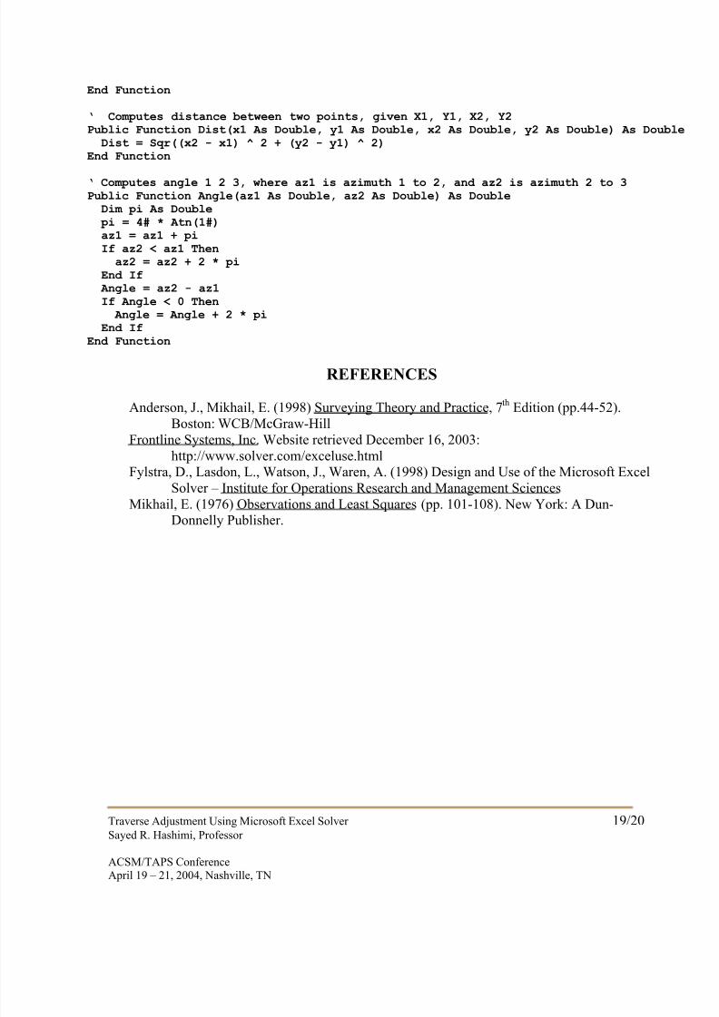
‘ Computes distance between two points, given X1, Y1, X2, Y2Public Function Dist(x1 As Double, y1 As Double, x2 As Double, y2 As Double) As DoubDist = Sqr((x2 - x1) ^ 2 + (y2 - y1) ^ 2)

End Function

‘ Computes angle 1 2 3, where az1 is azimuth 1 to 2, and az2 is azimuth 2 to 3Public Function Angle(az1 As Double, az2 As Double) As DoubleDim pi As Double

pi = 4# * Atn(1#)az1 = az1 + piIf az2 < az1 Thenaz2 = az2 + 2 * pi

End If Angle = az2 - az1If Angle < 0 Then Angle = Angle + 2 * piEnd If

End Function REFERENCES

Anderson, J., Mikhail, E. (1998) Surveying Theory and Practice, 7 th Edition (pp.44-52).Boston: WCB/McGraw-Hill

Frontline Systems, Inc. Website retrieved December 16, 2003:http://www.solver.com/exceluse.html

Fylstra, D., Lasdon, L., Watson, J., Waren, A. (1998) Design and Use of the Microsoft ExcelSolver – Institute for Operations Research and Management Sciences

Mikhail, E. (1976) Observations and Least Squares (pp. 101-108). New York: A Dun-Donnelly Publisher.





ACSM/TAPS Conference

BIOGRAPHICAL SKETCH

Sayed R. Hashimi is Professor and Department Chair of the Surveying EngineeringDepartment at Ferris State University. He is also a professional surveyor in the State of

Michigan. Professor Hashimi holds a masters degree in geodesy from Purdue University, a bachelor of technology degree in surveying from Oregon Institute of Technology formerlyknown as Oregon Technical Institute, and a bachelor of science degree in computer information systems from Ferris State University. He is the author of Ez-Adjust, acomprehensive least squares adjustment package for level network, two-D traverseadjustment including State Plane Coordinates option, three-D adjustment including GPS andterrestrial observations combined, four-parameter coordinate transformation, geoid modelingusing geoid 03 and much more. Information on Ez-Adjust can be obtained by visitinghttp://www.srh-leastsquares.com.

CONTACT

Sayed R. Hashimi, Professor Ferris State UniversitySurveying Engineering Department915 Campus Drive, Swan 314Big Rapids, MI 49307Phone: 231-591-2632e-mail: [email protected]

traverse adjustment using excel

Documents