Calhoun: The NPS Institutional Archive

DSpace Repository

Theses and Dissertations Thesis and Dissertation Collection

1986-09

Traverse adjustment.

Klangvichit, Supote

http://hdl.handle.net/10945/22159

Downloaded from NPS Archive: Calhoun

JDLEY KFOX LIBRARY""

kVAL P rE 3CH00LrtrtQ

ONTEREY, CALIFORNIA 9S943-B00S

NAVAL POSTGRADUATE SCHOOL

Monterey, California

THESISTRAVERSE ADJUSTMENT

by

Supote Klan gvlchit

September 1986

Thesis Co--Advi sors

:

MuneendGlen R.

ra

S

Kumar;haefer

Approved for public release; distribution is unlimited,

T231249

StCUHl I V CLASSIFICATION OF T"Hl5 PAGE

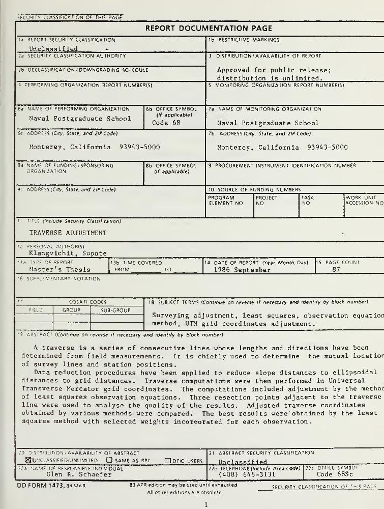
REPORT DOCUMENTATION PAGEla REPORT SECURITY CLASSIFICATION

Unclassified -lb RESTRICTIVE MARKINGS

2a SECURITY CLASSIFICATION AUTHORITY

2b DECLASSIFICATION /DOWNGRADING SCHEDULE

3 DISTRIBUTION/AVAILABILITY OF REPORT

Approved for public release;distr ibution i s unlimited.

4 PERFORMING ORGANIZATION REPORT NUMBER(S) 5 MONITORING ORGANIZATION REPORT NUMBER(S)

6a NAME OF PERFORMING ORGANIZATION

Naval Postgraduate School

6b OFFICE SYMBOL(If applicable)

Code 68

7a NAME OF MONITORING ORGANIZATION

Naval Postgraduate School

6< ADDRESS (Ofy. Sfafe. and ZlPCode)

Monterey, California 93943-5000

7b ADDRESS (Ofy, Sfafe, and ZlPCode)

Monterey, California 93943-5000

3a NAME OF FUNDING / SPONSORINGORGANIZATION

8b OFFICE SYMBOL(If applicable)

9 PROCUREMENT INSTRUMENT IDENTIFICATION NUMBER

8c ADDRESS (Ofy, Sfafe. and ZlPCode) 10 SOURCE OF FUNDING NUMBERS

PROGRAMELEMENT NO

PROJECTNO

TASKNO

WORK UNITACCESSION NO

title (include Security Claudication)

TRAVERSE ADJUSTMENT

PERSONAL AUTHOR(S)

Klangvichit, Supote

?j TYPE OF REPORT

Master's Thesis3b TIME COVEREDFROM TO

14 DATE OF REPORT (Year, Month, Day)

1986 September15 PAGE COUNT

87

6 SUPPLEMENTARY NOTATION

COSATl CODES

F ELD GROUP SUBGROUP

18 SUBJECT TERMS (Confmue on reverie if neceisary and identify by block number)

Surveying adjustment, least squares, observation equationmethod, UTM grid coordinates adjustment.

9 ABSTRACT (Confmue on reverie if neceisary and identify by block number)

A traverse is a series of consecutive lines whose lengths and directions have beendetermined from field measurements. It is chiefly used to determine the mutual location

of survey lines and station positions.Data reduction procedures have been applied to reduce slope distances to ellipsoidal

distances to grid distances. Traverse computations were then performed in UniversalTransverse Mercator grid coordinates. The computations included adjustment by the methodof least squares observation equations. Three resection points adjacent to the traverseline were used to analyse the quality of the results. Adjusted traverse coordinatesobtained by various methods were compared. The best results were obtained by the leastsquares method with selected weights incorporated for each observation.

">

r "'3UTiON/ AVAILABILITY OF ABSTRACT

^UNCLASSIFIED'-UNL'MITED D SAME AS RPT D DTIC USERS

21 ABSTRACT SECURITY CLASSIFICATION

Unclassified22a tjAMF OF RESPONSIBLE INDIVIDUAL

Glen R. Schaefer22b TELEPHONE (Include Area Code)

(408) 646-313122c OFFICE SYMBOL

Code 68Sc

DDFORM 1473.84MAR 83 APR edition may be used until exhausted

Alt other editions are obsoleteSECURITY CLASSIFICATION OF tmiS PAGE

Approved for public release; distribution is unlimited.

Traverse Adjustment

by

Supote KlangvichitLieutenant, Royal Thai Navy

B.S., Royal Thai Naval Academy, 1980

Submitted in partial fulfillment of the

requirements for the degree of

MASTER OF SCIENCE IN HYDROGRAPHIC SCIENCES

from the

NAVAL POSTGRADUATE SCHOOLSeptember 1986

ABSTRACT

A traverse is a series of consecutive lines whose lengths and directions have been

determined from field measurements. It is chiefly used to determine the mutual

location of survey lines and station positions.

Data reduction procedures have been applied to reduce slope distances to

ellipsoidal distances to grid distances. Traverse computations were then performed in

Universal Transverse Mercator grid coordinates. The computations included

adjustment by the method of approximation and by the method of least squares

observation equations. Three resection points adjacent to the traverse line were used

to analyse the quality of the results. Adjusted traverse coordinates obtained by various

methods were compared. The best results were obtained by the least squares method

with selected weights incorporated for each observation.

12$ l*

TABLE OF CONTENTS

I. INTRODUCTION 8

A. BACKGROUND 8

B. OBJECTIVES 9

II. TRAVERSES 10

A. GENERAL 10

1

.

Open Traverse 10

2. Closed Traverse 11

B. ANGULAR AND DIRECTIONAL MEASUREMENTS 11

1. Interior Angle 12

2. Deflection Angle 12

3. Angle To The Right 12

C. LINEAR MEASUREMENT 13*

D. ACCURACY 14

E. ADJUSTMENTS 15

1. Approximation Methods 15

2. Adjustment by Least Squares Method 17

III. DATA ACQUISITION AND REDUCTION 22

A. DATA ACQUISITION 22

B. DATA REDUCTION 22

1. Computation of Ellipsoidal Distances 22

2. Computation of Geodetic Distances 24

3. Reduction of Horizontal Distances to Geodetic Distances 29

C. GRID DISTANCES 29

IV. TRAVERSE COMPUTATION AND ADJUSTMENT 31

A. DATA PROCESSING 31

1. Set up of data base 31

2. Modification of an Existing Program 31

3. Writing a New Program 31

B. COMPUTATION OF STARTING AND CLOSINGAZIMUTHS 31

C. COMPUTATION OF TRAVERSE STATIONCOORDINATES 34

D. ADJUSTMENT BY APPROXIMATION METHOD 36

1. Angular Errors of Closure 36

2. Linear Errors of Closure 36

E. LEAST SQUARES ADJUSTMENT BY OBSERVATIONEQUATIONS 37

V. ANALYSIS OF RESULTS 46

A. COMPARISON OF ADJUSTED COORDINATES 46

B. ANALYSIS OF THE REFERENCE VARIANCE OFUNIT WEIGHT 47

VI. CONCLUSIONS AND RECOMMENDATIONS 50

A. CONCLUSIONS 50

B. RECOMMENDATION 50

APPENDIX A: LINEARIZATIONS 51

APPENDIX B: TRAVADJ FORTRAN PROGRAM 52

APPENDIX C: INDTRA FORTRAN PROGRAM 64

LIST OF REFERENCES 84

INITIAL DISTRIBUTION LIST 85

LIST OF TABLES

I. TRAVERSE CLASSIFICATION 16

II. DATA OF KNOWN STATIONS 24

III. OBSERVED HORIZONTAL ANGLES 25

IV. MEASURED DISTANCES AND GRID DISTANCES 26

V. SPECIFICATION OF PARAMETERS 30

VI. QUADRANT OF AZIMUTH 33

VII. UNADJUSTED TRAVERSE STATION POSITIONS 35

VIII. TRAVERSE CLOSURE 38

IX. LATITUDE AND DEPARTURE CORRECTIONS 38

X. ADJUSTED COORDINATES BY COMPASS RULE 39

XI. THE COEFFICIENTS OF ANGLE AND DISTANCECONDITIONS 43

XII. ADJUSTED COORDINATES BY OBSERVATIONEQUATION 44

XIII. ADJUSTED STANDARD DEVIATION OF ANGLES ANDDISTANCES 45

XIV. COMPARISON OF ADJUSTEDCOORDINATES'DISTANCES OBTAINED BYAPPROXIMATION AND LEAST SQUARES METHODS 47

XV. COMPARISON OF COORDINATES AT INTERSECTIONPOINTS 49

XVI. COMPARISION OF VARIANCES OF UNIT WEIGHT 49

LIST OF FIGURES

2.

1

Open Traverse 10

2.2 Closed-loop Traverse 11

2.3 Closed-connecting Traverse 12

2.4 Measuring of Interior Angles 13

2.5 Measuring of Deflection Angles 13

2.6 Measuring of Angles to the Right 14

3.1 Traverse Layout 23

3.2 Ellipsoidal Distance 26

3.3 Slope Reduction for Typical Triangle 27

4.1 Azimuth Computation 33

4.2 Determination of Angle and Distance from Coordinates 41-

5.1 Comparison of Adjusted Distances Obtained by Approximation andLeast Squares Methods 4$-

I. INTRODUCTION

A. BACKGROUNDSurveying is the science and art of measurements which are necessary to

determine the relative position of points above, on, or beneath the surface of the earth,

or to establish the points in a specified position. Surveying operations are conducted

not only on land, but also in the oceans and in space. The measurements of surveying

consist of distances, horizontal and vertical, and directions. In order to provide a

framework of survey points whose horizontal and vertical positions are accurately

known, basic horizontal and vertical control surveys must be performed. A primary

use of control surveys is for construction of control for a map or chart. The

fundamental network of points whose horizontal positions have been accurately

determined is called horizontal control [Schmidt, 1978, p. 122].

Horizontal control generally is established either by traverse, triangulation, or

trilateration. Which one is to be used depends on the accuracy required and the factor

of economy in the selection of survey method. Obviously, there are many degrees of

precision possible in any measurement because no surveying measurement is exact.

Each of these methods may be the best one to use for a given purpose. Ordinarily, it is

a waste of time and money to attain unnecessarily high accuracy. On the other hand,

if the measurements are not sufficiently precise, faulty survey results are produced.

Therefore, the best surveyor is not the one who makes the most precise measurements,

but the one who is able to choose and apply the appropriate measurement with

precision requisite to the purpose.

Before 1950 the main framework of a first-order geodetic survey almost always

consisted of triangulation, which could be replaced by traverse in cases where the

topography made triangulation impracticable. Today, due to the development of

electronic distance measuring (EDM) equipment, the first-order control points can be

established by means of high accuracy traverse [Allan, 1968, p. 370]. Therefore, the

horizontal control is frequently provided by traverse, especially for surveys in area of

limited extent, mostly flat and jungle covered. Traverse in such cases is much more

economic, convenient, and rapid than other methods and the results are equally

accurate.

In order to achieve high precision of horizontal control points when distributed

over a large area, first or second-order geodetic surveys are required. These types of

survey treat the shape of the earth as ellipsoidal and require using the most accurate

distance and angle measurements. Computation of such a survey is relatively

complicated, based on long geodetic formulas for computing (with necessary precision)

the exact horizontal and vertical position of widely distributed points on the earth's

surface.

Disregarding ellipsoid shape, a third-order survey is used over earth areas of

limited extent. In this type of a survey, the earth can be considered as fiat and all

angles are considered to be plane angles. Surveys of this type are used in the

dcnsification of geodetic control.

B. OBJECTIVES

As mentioned above, the traverse method has been used worldwide mostly for

densification of control stations. However, there are many methods of traverse

computations. The main objectives of this thesis are to (1) compute a

closed-connecting traverse and adjust station positions by the Approximation Method *

with the compass (Bowditch) rule and Least Squares Method (adjustment by

observation equations only), and (2) compare the results of the two methods.

All computations have been accomplished in the Universal Transverse Mercator

(UTM) grid coordinates rather than geodetic coordinates.

II. TRAVERSES

A. GENERAL

The word traverse generally means to pass across. But in surveying, this word

means the measurement in a specified sequence of the lengths and directions of lines

between points on the earth whose position may be know or unknown. Traverse is the

most widely employed method for dcnsification of local horizontal control. Linear

measurements are made either by direct observation using a tape or ISDM equipment,

or by indirect observation using tachcomctric methods. The angular measurements arc

made with theodolite or transit. In this thesis, the only traverse operations considered

arc for angles measured by theodolite and distances measured by precise I:DM

equipment or tapes.

Two kinds of traverse exist in surveying, an open and a closed traverse.

1. Open Traverse

An open traverse normally originates at a point of known position and docs

not return to the starting point nor docs it terminate on another point of known

position (figure 2.1). Open traverses should generally not be used because they can

not be checked for errors.

Ao

= known station

= unknown station

= measured distance= observed angle

A'o

Figure 2.1 Open Traverse.

10

2. Closed Traverse

Closed traverses can further be sub-divided as, a closed-loop and a

closed-connecting traverse.

A closed-loop traverse is one that originates and terminates on a single point

of known position, thus forming a closed polygon (figure 2.2). This type of traverse

provides an internal check on angles but no check on systematic errors in distance.

Also, if the starting azimuth (between stations and 1 in figure 2.2 ) has an error, it

causes error in orientation of the entire traverse. A closed-loop traverse generally

should not be used.

A = known station

pto = unknown station

= measured distance ^>^

3 i JA = observed angle

XvV6

L 3

/ *4 A \\i

6<&J Ky

Figure 2.2 Closed-loop Traverse.

A closed-connecting traverse is one that begins and ends on two different

points whose horizontal positions have been previously determined by a survey of

higher or equal accuracy (Figure 2.3). This type of traverse is preferable to all others,

since computational checks are possible to detect systematic errors in both distance

and direction.

B. ANGULAR AND DIRECTIONAL MEASUREMENTSThe position of traverse points is determined by the direction and distance from

the starting point. To obtain the direction by means of azimuth, the horizontal angle,

or plane angle, must be measured in the field. Also, the determination of vertical

angles, or zenith distances, may be required to reduce slope distances to horizontal

distances.

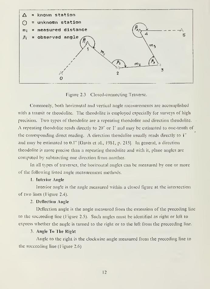
A = known station

O = unknown station

mi = measured distance

Pi - observed angle

A

Figure 2.3 Closed-connecting Traverse.

Commonly, both horizontal and vertical angle measurements are accomplished

with a transit or theodolite. The theodolite is employed especially for surveys of high

precision. Two types of theodolite are a repeating theodolite and direction theodolite. -

A repeating theodolite reads directly to 20" or V and may be estimated to one-tenth of

the corresponding direct reading. A direction theodolite usually reads directly to 1"

and may be estimated to 0.1" [Davis et al., 1981, p. 215]. In general, a direction

theodolite is more precise than a repeating theodolite and with it, plane angles are

computed by subtracting one direction from another.

In all types of traverses, the horizontal angles can be measured by one or more

of the following listed angle measurement methods.

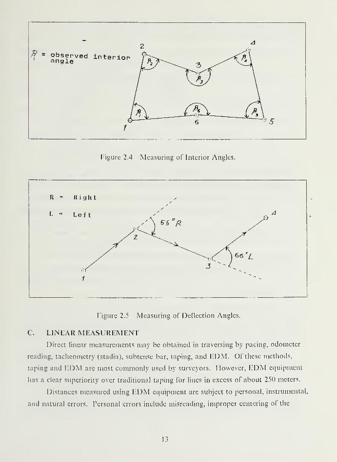
1. Interior Angle

Interior angle is the angle measured within a closed figure at the intersection

of two lines (Figure 2.4).

2. Deflection Angle

Deflection angle is the angle measured from the extension of the preceding line

to the succeeding line (Figure 2.5). Such angles must be identified as right or left to

express whether the angle is turned to the right or to the left from the precceding line.

3. Angle To The Right

Angle to the right is the clockwise angle measured from the preceding line to

the succeeding line (Figure 2.6)

12

24

H ~ observed interiorf^\ /<^

1

6A\'"5

Figure 2.4 Measuring of Interior Angles.

Figure 2.5 Measuring of Deflection Angles.

C. LINEAR MEASUREMENTDirect linear measurements may be obtained in traversing by pacing, odometer

reading, tachcomctry (stadia), subtense bar, taping, and EDM. Of these methods,

taping and EDM are most commonly used by surveyors. However, FDM equipment

has a clear superiority over traditional taping for lines in excess of about 250 meters.

Distances measured using FDM equipment are subject to personal, instrumental

and natural errors. Personal errors include misreading, improper centering of the

I3

Figure 2.6 Measuring of Angles to the Right.

instrument over the stations, failing to exactly center the null meter, and incorrectly

measuring meteorological factors and instrument heights. Instrumental errors,

expressed in terms of the accuracy of the instrument specified by the manufacturer,

contain two parts. For example, if the accuracy of an instrument is designated as ±

(K) ppm + 5 mm), the constant error part is + 5 mm, which is independent of the

distance, and the value of the proportional part is 10 ppm (parts per million) which is a

function of the distance measured. Constant error is most significant for short

distances. For very long distances the constant error becomes negligible, but the

proportional part is important. Natural errors such as refraction are cause by

changing of atmospheric conditions along the measured line between the end stations.

D. ACCURACY

In survey adjustment, a deviation from the 'true' value is considered as an

observational error and the standard error designates the measure of accuracy of the

observation. The meaning of an accuracy is then the degree of conformity or closeness

of a measurement to true value.

The quality of traverse operations is dependent upon the accuracy of angular and

linear measurements; thus, in checking the accuracy of traverse two quantities are

considered, the angular misclosure and the linear misclosure. Although the positional

closure (relative accuracy) is an indication of the overall quality of the traverse and is

used for traverse classification, it docs not yield information on the precision of point

location determined in a traverse [Davis ct al., p. 332].

14

The inherent weakness in a traverse is that the deviation of each measured line is

determined by a siftgle series of angular observations, further, any error in any angle

will affect not only the adjoining line but all subsequent lines to a greater or lesser

extent according to their lengths [Allan, 1968, p. 371].

Angular misclosure is expressed by standard error of the measured angle times

the square root of the number of measured angles.

Linear misclosure is commonly expressed as a ratio of total misclosure to total

length of traverse.

Finally, some of the most significant features of traverse classification by the U.S.

Federal Geodetic Control Committee (1984) are shown in Table I.

E. ADJUSTMENTS

Adjustment of a traverse is carried out to ensure consistency within the known

positions of the originating and terminating stations and to remove inconsistencies in

observed angles and distances to compensate for random errors. For a more precise

extended traverse, adjustments made on the basis of least squares are preferred. But a

traverse of limited extent can be adjusted by simple approximation methods.

1. Approximation Methods

There are four methods for traverse adjustment by approximation.

a. Arbitary Method

This method does not conform to a fixed rule. Rather, the linear error of

closure is distributed arbitarily according to arbitary preference of the surveyor.

b. Transit Rule

Transit rule is better for adjustment of the traverse where the angles are

measured with greater accuracy than distances, and is valid only when the traverse lines

are parallel with the grid system used for the traverse computations. Corrections are

made by the following rules: the correction in latitude for any station is equal to the

multiple of latitude in that section and total closure in latitude divided by the sum of

all latitudes in traverse, and the correction in departure is equal to the multiple of

departure in that section and total closure in departure divided by the sum of all

departures in the traverse [Davis et al., 1981, p. 323].

c. Compass or Bowditch Rule

This method is suitable for adjustment of the traverse where the angles and

distances are measured with equal precision and uses the following rules: the correction

15

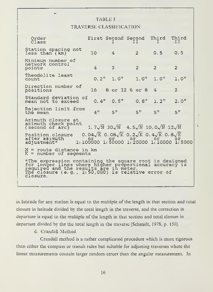
TABLE I

TRAVERSE CLASSIFICATION

Order First Second Second Third ThirdClass I II I II

Station spacing notless than (km) 10 4 2 0. 5 0. 5

Minimum number ofnetwork controlpoints 4 3 2 2 2

Theodolite leastcount 0.2" 1.0" 1.0" 1.0" 1.

Direction number ofpositions 16 8 or 12 6 or 8 4 2

Standard deviation ofmean not to exceed 0.4" 0.5" 0.8" 1.2" 2.

Rejection limit fromthe mean 4" 5" 5" 5" 5"

0"

0"

Azimuth closure atazimuth check point _» , , . .

( second of arc) 1. 7VN 30VN 4. 5VN 10. 0^N 12VN

Position closure 0.04^ 0. 08Vk 0. 2^K 0. 4^K 0.8^after azimuth or or or or oradjustment* 1:100000 1:50000 1:20000 1:10000 1:5000

N = route distance in kmK = number of segments

*The expression containing the square root is designedfor longer lines where higher proportional accuracy isrequired and the results are in meter.The closure (e.g., 1:50,000) is relative error ofclosure.

in latitude for any station is equal to the multiple of the length in that section and total

closure in latitude divided by the total length in the traverse, and the correction in

departure is equal to the multiple of the length in that section and total closure in

departure divided by the the total length in the traverse [Schmidt, 1978, p. 150].

d. Crandall Method

Crandall method is a rather complicated procedure which is more rigorous

than either the compass or transit rules but suitable for adjusting traverses where the

linear measurements contain larger random errors than the angular measurement. In

16

this method, the angular error of closure is first distributed in equal portions to all of

the measured angles, then linear measurements are adjusted by using a weighted least

squares procedure [Brinker, 1977, p. 228].

2. Adjustment by Least Squares Method

The method of least squares adjustment is based upon the theory of

probability; it simultaneously adjusts the angular and linear measurements to make the

sum of the square of the residuals (error) a minimum [Brinker, 1977, p. 228]. This

method can be used for any type of traverse. Because of the availibility of fast

computing devices at the present time, the least squares method is being widely used.

Further, the least squares solution has the advantage that it determines, quite

objectively, a unique solution for a given adjustment problem [Clark, 1973, p. 121].

In general, adjustment is needed whenever there are redundant observations

(more observations than are necessary to solve the required unknowns). As an

example, to determine the angles of a plane triangle, only two observed angles are

required because the third angle can be obtained by subtraction from 180°. When

three angles are observed, the sum of them will not be equal 180° due to error in

measurements. Therefore, these three angles should be adjusted to fit the functional

model.

The redundancy may be interpreted to mean that among n observations there

exist r conditions or functions (n > r) that must satisfy the model.

Let n be a number of observations and t\q the minimum number of

observations to find the uniquely solution in the model, then redundancy or degree of

freedom in the statistic, r, is

r = n - n (2.1)

Consequently, there are r redundant observations, which can also give a

solution. To detect the error in each observation, the best estimated or the most

probable value must be defined because the true value is not known exactly.

Statistically, the best estimated value of a group of repeated observation is the average

(arithmetic mean).

Once the difference between observed value (X_) and estimated value (Xe) is

determined, the adjusted value (X ) is obtained through a least squares solution, then

the residual (v) can be expressed as

17

v = Xa-X (2.2)

and

Xa= X

e+ dx (2.3)

where dx is the correction to estimated value to obtain the adjusted value.

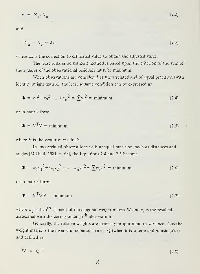
The least squares adjustment method is based upon the criterion of the sum of

the squares of the observational residuals must be minimum.

When observations are considered as uncorrelated and of equal precision (with

identity weight matrix), the least squares condition can be expressed as

<P = vi+v2 + -- + v

n= X v

i

= minimum (2.4)

or in matrix form

(p = yTV = minimum (2.5)

where V is the vector of residuals.

In uncorrelated observations with unequal precision, such as distances and

angles [Mikhail, 1981, p. 68], the Equations 2.4 and 2.5 become

= WjVj +W2V2 + --- + wnvn Xwiv

i

= minimum (2.6)

or in matrix form

d) = vTWV = minimum (2.7)

where w- is the ith

element of the diagonal weight matrix W and v- is the residual

associated with the corresponding i observation.

Generally, the relative weights are inversely proportional to variance, thus the

weight matrix is the inverse of cofactor matrix, Q (when it is square and nonsingular)

and defined as

W = Q' 1

(2.8)

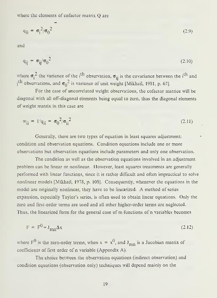
where the elements of cofactor matrix Q are

% = °?l°02

(2-9)

and

% = aij/<T

2(2-10)

where <r-2the variance of the i

thobservation, a-- is the covariance between the i

th and

j

mobservations, and <7q

Zis variance of unit weight [Mikhail, 1981, p. 67].

For the case of uncorrected weight observations, the cofactor matrice will be

diagonal with all off-diagonal elements being equal to zero, thus the diagonal elements

of weight matrix in this case are

wii= l '%= ff

2/*ii

2(2.11)

Generally, there are two types of equation in least squares adjustment:

condition and observation equations. Condition equations include one or more

observations but observation equations include parameters and only one observation.

The condition as well as the observation equations involved in an adjustment

problem can be linear or nonlinear. However, least squares treatments are generally

performed with linear functions, since it is rather difficult and often impractical to solve

nonlinear models [Mikhail, 1978, p. 108]. Consequently, whenever the equations in the

model are originally nonlinear, they have to be linearized. A method of series

expansion, especially Taylor's series, is often used to obtain linear equations. Only the

zero and first-order terms are used and all other higher-order terms are neglected.

Thus, the linearized form for the general case of m functions of n variables becomes

F = F° + JmnAx < 2 - 12 )

where F is the zero-order terms, when x = x , and J is a Jacobian matrix of

coefficients of first order of n variable (Appendix A).

The choice between the observation equations (indirect observation) and

condition equations (observation only) techniques will depend mainly on the

19

mathematical model of the problem to be solved. However, the final answers are

always the same.

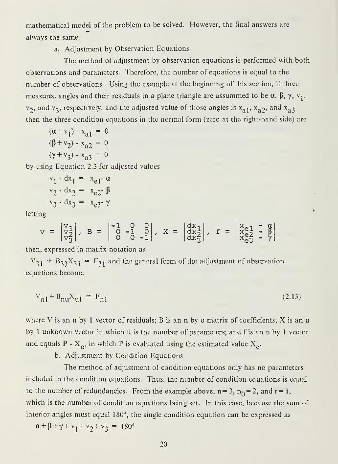
a. Adjustment by Observation Equations

The method of adjustment by observation equations is performed with both

observations and parameters. Therefore, the number of equations is equal to the

number of observations. Using the example at the beginning of this section, if three

measured angles and their residuals in a plane triangle are assummed to be a, P, y, Vj,

V2, and v3

, respectively, and the adjusted value of those angles is xa j, xa2 , and x

a3

then the three condition equations in the normal form (zero at the right-hand side) are

(a + v1)-x

al=

(P + v2)-xa2 =

(Y + v3 ) ^a3

=

by using Equation 2.3 for adjusted values

1dxj = xeF a

2" dX') = xe2" P

3"dx 3= x

e3_ Y

letting

v = B =-1

-1dx-idx*dx§

1-1

, x =, f = el

e2

- a-

P

e3 " y

then, expressed in matrix notation as

V31

+ B33X31

equations become

^31 + B33X 31

= F31 and the general form of the adjustment of observation

Vnl

+ BnuXul ~ Fnl (2.13)

where V is an n by 1 vector of residuals; B is an n by u matrix of coefficients; X is an u

by 1 unknown vector in which u is the number of parameters; and f is an n by 1 vector

and equals P - XQ , in which P is evaluated using the estimated value X

e>

b. Adjustment by Condition Equations

The method of adjustment of condition equations only has no parameters

included in the condition equations. Thus, the number of condition equations is equal

to the number of redundancies. From the example above, n= 3, nQ= 2, and r= 1,

which is the number of condition equations being set. In this case, because the sum of

interior angles must equal 180°, the single condition equation can be expressed as

a + p + Y + vj + V2+ v3= 180°

20

r

l+ v2+v3

= 180° -a - P - y

A =| 1,1,1 |, V = Zi

7r2v3

Then, the general form of this technique is

F =| 180-a-P-y

ArnVnr

= Frl

(2.14)

When the conditions are originally linear, the vector F is usually written in terms of the

given observations as

Frl " P

rl " ArnXo,nl (2.15)

where A is the coefficient matrix V., P is a constant term (see Section II. E. a), X Qis

observed values, r is redundancy, and n is a number of observation [Mikhail, 1976, p.

173].

21

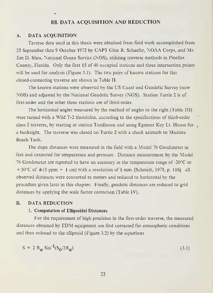
III. DATA ACQUISITION AND REDUCTION

A. DATA ACQUISITION

Taverse data used in this thesis were obtained from field work accomplished from

25 September thru 9 October 1972 by CAPT Glen R. Schaefer, NOAA Corps, and Mr.

Jim D. Shea, National Ocean Service (NOS), utilizing traverse methods in Pinellas

County, Florida. Only the first 15 of 40 occupied stations and three intersection points

will be used for analysis (Figure 3.1). The two pairs of known stations for this

closed-connecting traverse are shown in Table II.

The known stations were observed by the US Coast and Geodetic Survey (now

NOS) and adjusted by the National Geodetic Survey (NGS). Station Turtle 2 is of

first-order and the other three stations are of third-order.

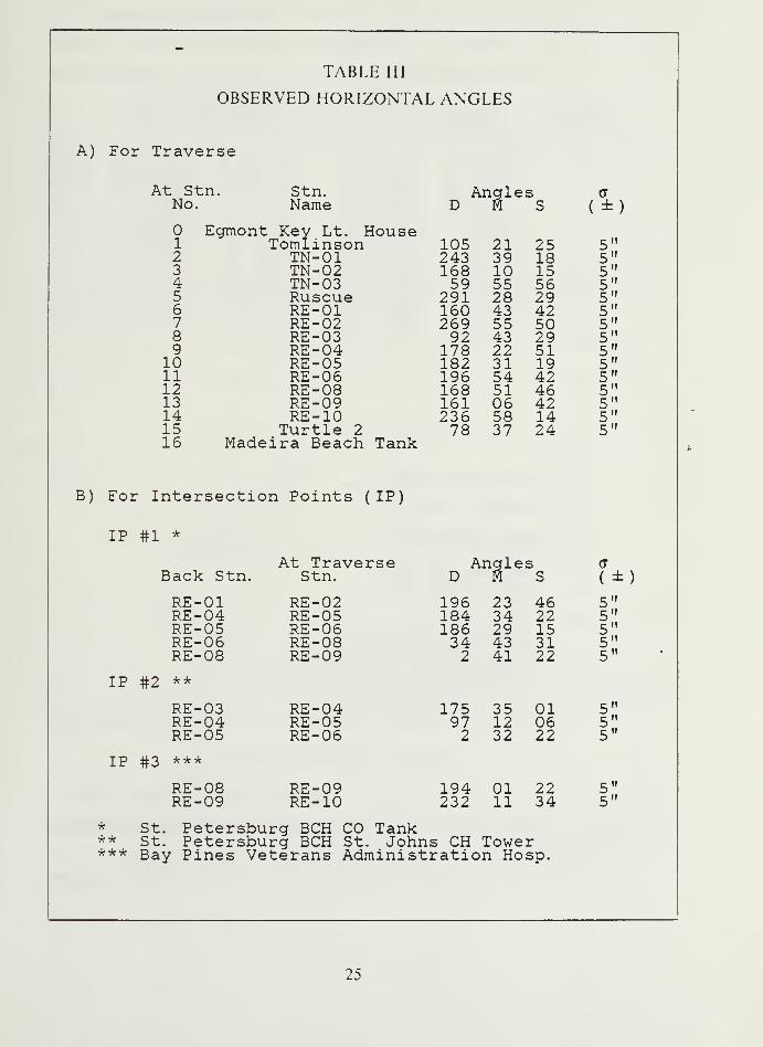
The horizontal angles measured by the method of angles to the right (Table III)

were turned with a Wild T-2 theodolite, according to the specifications of third-order

class I traverse, by starting at station Tomlinson and using Egmont Key Lt. House for t

a backsight. The traverse was closed on Turtle 2 with a check azimuth to Madeira

Beach Tank.

The slope distances were measured in the field with a Model 76 Geodimeter in

feet and corrected for temperature and pressure. Distance measurement by the Model

76 Geodimeter are reported to have an accuracy in the temperature range of -20°C to

+ 50°C of ±(1 ppm + 1 cm) with a resolution of 1 mm. [Schmidt, 1978, p. 116]. all

observed distances were converted to meters and reduced to horizontal by the

procedure given later in this chapter. Finally, geodetic distances are reduced to grid

distances by applying the scale factor correction (Table IV).

B. DATA REDUCTION

1. Computation of Ellipsoidal Distances

For the requirement of high precision in the first-order traverse, the measured

distances obtained by EDM equipment are first corrected for atmospheric conditions

and then reduced to the ellipsoid (Figure 3.2) by the equations

S = 2Ra Sin-1(S /2Ra) (3.1)

22

re

A = known station

O = traverse stationIP = intersection point

IP 5

T'^-o 11

Nor TO Scali

Figure 3.1 Traverse Layout.

23

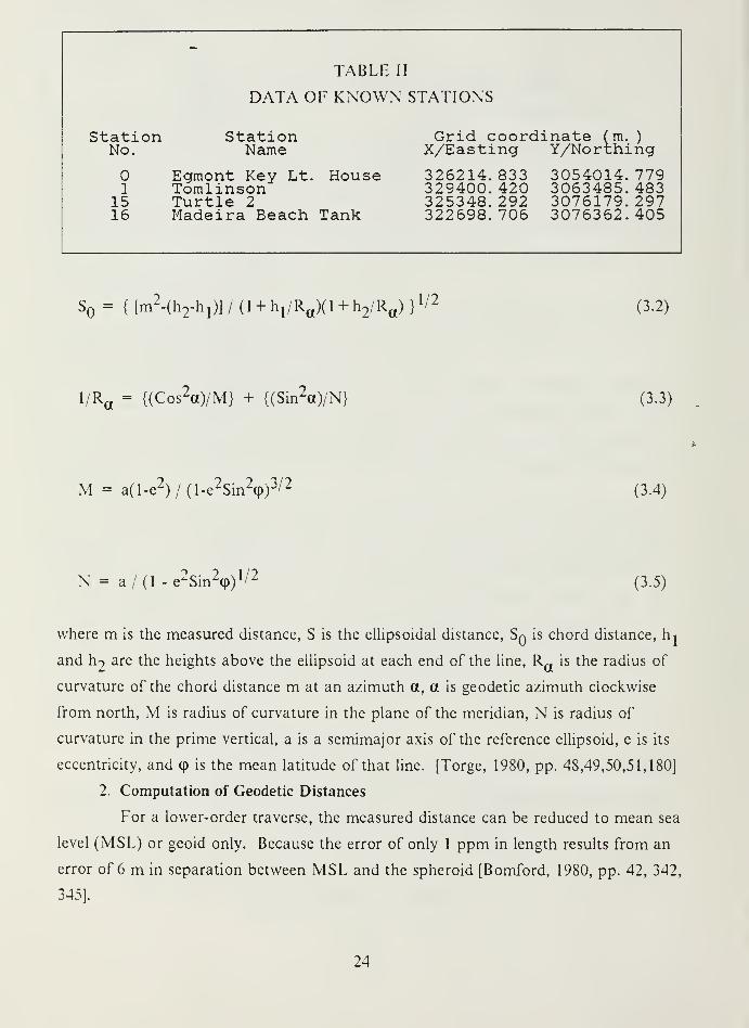
TABLE II

DATA OF KNOWN STATIONS

StationNo.

Station Grid coordinate ( m. )

Name X/Easting Y/Northing

11516

Egmont Key Lt. House 326214.833 3054014.Tomlinson 329400.420 3063485.Turtle 2 325348.292 3076179.Madeira Beach Tank 322698.706 3076362.

779483297405

S = {[m2-(h

2-h

1)]/(l + h

1/Ra )(l + h

2/Ra)}

1 / 2 (3.2)

1/Ra= {(Cos2a)/M} + {(Sin

2a)/N} (3.3)

M = a(l-e2)/(l-e2Sin2(p)

3 / 2 (3.4)

N = a/(l - e2Sin

2<p)

1 /2 (3.5)

where m is the measured distance, S is the ellipsoidal distance, Sq is chord distance, hj

and h2

are the heights above the ellipsoid at each end of the line, Ra is the radius of

curvature of the chord distance m at an azimuth a, a is geodetic azimuth clockwise

from north, M is radius of curvature in the plane of the meridian, N is radius of

curvature in the prime vertical, a is a semimajor axis of the reference ellipsoid, e is its

eccentricity, and (p is the mean latitude of that line. [Torge, 1980, pp. 48,49,50,51,180]

2. Computation of Geodetic Distances

For a lower-order traverse, the measured distance can be reduced to mean sea

level (MSL) or geoid only. Because the error of only 1 ppm in length results from an

error of 6 m in separation between MSL and the spheroid [Bomford, 1980, pp. 42, 342,

345].

24

—

TABLE III

OBSERVED HORIZONTAL ANGLES

A) For Traverse

At Stn. Stn. Ancrles (T

No. Name D H S ( ±)Egmont Key Lt. House

1 Tomlinson 105 21 25 5"2 TN-01 243 39 18 5"3 TN-02 168 10 15 5"4 TN-03 59 55 56 5"5 Ruscue 291 28 29 5"6 RE-01 160 43 42 5"7 RE-02 269 55 50 5"8 RE-03 92 43 29 5"9 RE-04 178 22 51 5"

10 RE-05 182 31 19 5"11 RE-06 196 54 42 5"12 RE-08 168 51 46 5"13 RE-09 161 06 42 5"14 RE-10 236 58 14 5"15 Turtle 2 78 37 24 5"16 Madeira Beach Tank

B) For Intersection Points ( IP)

IP #1 *

At Traverse Ancrles (7

Back Stn. Stn. D K S ( ±)

RE-01 RE-02 196 23 46 5"RE-04 RE-05 184 34 22 5"RE-05 RE-06 186 29 15 5"RE-06 RE-08 34 43 31 5"RE-08 RE-09 2 41 22 5"

IP #2 **

RE-03 RE-04 175 35 01 5"RE-04 RE-05 97 12 06 5"RE-05 RE-06 2 32 22 5"

IP #3 ***

RE-08 RE-09 194 01 22 5"RE-09 RE-10 232 11 34 5"

* St. Petersburg BCH CO Tankx k St. Petersburg BCH St. John s CH Towe r*** Bay Pines Veterans Administration Ho sp.

25

TABLE IV

MEASURED DISTANCES AND GRID DISTANCES

At Stn. Measured Distances Grid Distances (T

To Stn. ft m ft m (tm)

1 2300. 98 701. 340 2300. 91 701. 318 0. 0172 2605. 41 794. 131 2605. 28 794. 090 0. 0183 4452. 48 1357. 119 4452. 31 1357. 068 0. 0244 709. 56 216. 274 709. 54 216. 267 0. 0125 5050. 37 1539. 356 5050. 21 1539. 307 0. 0256 6620. 54 2017. 945 6620. 33 2017. 880 0. 0307 1655. 17 504. 497 1655. 12 504. 481 0. 0158 1605. 85 489. 464 1605. 80 489. 448 0. 0159 2114. 68 644. 556 2114. 61 644. 535 0. 016

10 2362. 13 719. 979 2362. 05 719. 956 0. 01711 1360. 16 414. 578 1360. 10 414. 561 0. 01412 5060. 98 1542. 590 5060. 41 1542. 415 0. 02513 6172. 26 1881. 309 6171. 67 1881. 128 0. 02914 6664. 72 2031. 411 6664. 51 2031. 346 0. 03015

m - measured distance V^~—^n>So

s =

chord distance V\A

arc distance on V=ellipsoid \

S^=S/k

s<,

»1

h a=

elevation above ^

ellipsoid atstation 1

elevation aboveellipsoid at station 2

/r«

R~ radius earth curvaturealong measured line

Figure 3.2 Ellipsoidal Distance.

However, the process of reduction requires three steps: (1) correct slope

distances to horizontal distances, (2) reduce horizontal distance to geodetic distances,

and (3) change the geodetic distances to grid distances.

'I he slope distance data used included correction for atmospheric conditions.

26

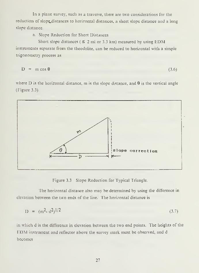
In a plane survey, such as a traverse, there are two considerations for the

reduction of slopojdistances to horizontal distances, a short slope distance and a long

slope distance.

a. Slope Reduction for Short Distances

Short slope distances (< 2 mi or 3.3 km) measured by using EDM

instruments separate from the theodolite, can be reduced to horizontal with a simple

trigonometry process as

D = m cos 9 (3.6)

where D is the horizontal distance, m is the slope distance, and is the vertical angle

(Figure 3.3).

[slope correctionU ._ "^ «-,

r V

Figure 3.3 Slope Reduction for Typical Triangle.

The horizontal distance also may be determined by using the difference in

elevation between the two ends of the line. The horizontal distance is

D = (m2- d 2

)

1 '' 2(3.7)

in which d is the difference in elevation between the two end points. The heights of the

EDM instrument and reflector above the survey mark must be observed, and d

becomes

27

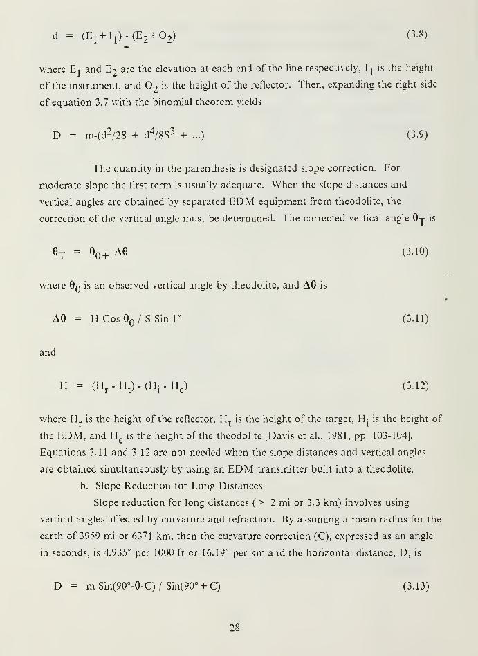
d = (E1+ I

1)-(E2+02) (3.8)

where Ej and E2are the elevation at each end of the line respectively, Ij is the height

of the instrument, and2

is the height of the reflector. Then, expanding the right side

of equation 3.7 with the binomial theorem yields

D = m-(d2/2S + d4/8S 3 + ...) (3.9)

The quantity in the parenthesis is designated slope correction. For

moderate slope the first term is usually adequate. When the slope distances and

vertical angles are obtained by separated EDM equipment from theodolite, the

correction of the vertical angle must be determined. The corrected vertical angle Qj is

GT = 90+ AG (3.10)

where 9q is an observed vertical angle by theodolite, and AG is

AG = H CosG / S Sin 1" (3.11)

and

H = (Hr

- Ht) - (^ - H

e)(3.12)

where Hr

is the height of the reflector, Ht

is the height of the target, H- is the height of

the EDM, and He

is the height of the theodolite [Davis et al., 1981, pp. 103-104].

Equations 3.11 and 3.12 are not needed when the slope distances and vertical angles

are obtained simultaneously by using an EDM transmitter built into a theodolite,

b. Slope Reduction for Long Distances

Slope reduction for long distances (> 2 mi or 3.3 km) involves using

vertical angles affected by curvature and refraction. By assuming a mean radius for the

earth of 3959 mi or 6371 km, then the curvature correction (C), expressed as an angle

in seconds, is 4.935" per 1000 ft or 16.19" per km and the horizontal distance, D, is

D = m Sin(90°-G-C) / Sin(90° + C) (3.13)

28

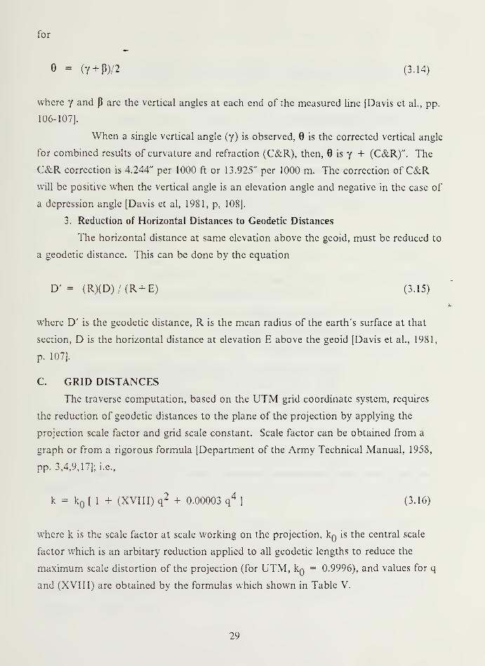
for

6 = (Y + P)/2 (3.14)

where y and are the vertical angles at each end of the measured line [Davis et al, pp.

106-107].

When a single vertical angle (y) is observed, is the corrected vertical angle

for combined results of curvature and refraction (C&R), then, G is y + (C&R)". The

C&R correction is 4.244" per 1000 ft or 13.925" per 1000 m. The correction of C&Rwill be positive when the vertical angle is an elevation angle and negative in the case of

a depression angle [Davis et al, 1981, p, 108].

3. Reduction of Horizontal Distances to Geodetic Distances

The horizontal distance at same elevation above the geoid, must be reduced to

a geodetic distance. This can be done by the equation

D' = (R)(D)/(R+E) (3.15)

where D' is the geodetic distance, R is the mean radius of the earth's surface at that

section, D is the horizontal distance at elevation E above the geoid [Davis et al., 1981,

p. 107].

C. GRID DISTANCES

The traverse computation, based on the UTM grid coordinate system, requires

the reduction of geodetic distances to the plane of the projection by applying the

projection scale factor and grid scale constant. Scale factor can be obtained from a

graph or from a rigorous formula [Department of the Army Technical Manual, 1958,

pp. 3,4,9,17]; i.e.,

k = kQ [ 1 + (XVIII) q

2 + 0.00003 q4

] (3.16)

where k is the scale factor at scale working on the projection, k^ is the central scale

factor which is an arbitary reduction applied to all geodetic lengths to reduce the

maximum scale distortion of the projection (for UTM, kQ = 0.9996), and values for q

and (XVIII) are obtained by the formulas which shown in Table V.

29

TABLE V

SPECIFICATION OF PARAMETERS

XVIII =1 + e' Cos2 (p . 1 . 10 12

2 v2 k^"

V =a

( 1 - ez Sin2^)1/2

e2 = (ecentricity) 2 = ( a2 - b2 ) / a2

e 2 ' = e 2 / (1 - e 2)

q = 0. 000001 E'

E = grid easting = E' + 500,000 when point iseast of central meridian, 500,000 - Ewhen point is west of central meridian

V = radius of curvature in the prime vertical

a = semi-major axis of the ellipsoid

b = semi-minor axis of the ellipsoid

<P= latitude

30

IV. TRAVERSE COMPUTATION AND ADJUSTMENT

Linear measurements and angles must be checked by computation to determine

the position of traverse stations and whether the traverse meets required precision.

Traverse station coordinates are usually expressed in terms of geographical coordinates

or rectangular coordinates such as those based on an UTM projection. Traverse

computations are usually done in rectangular coordinates because of the ease of

computation. In this thesis, only closed-connecting traverse computations in UTMcoordinates were used. When specifications were satisfied, the traverse was adjusted

for perfect geometric consistency among angles and lengths.

A. DATA PROCESSING

1. Set up of data base

Two files on IBM 370/3033AP main frame computer at NPS were established.

2. Modification of an Existing Program

The Fortran program TRAVADJ, originally written by LCDR Saman

Aumchantr, RTN (1984) in Watfiv language for computing and adjusting the traverse

station coordinates, was modified to be able to handle the distances reduction

processes.

3. Writing a New Program

A Fortran program INDTRA was written for computing and simultaneously

adjusting traverse station and intersection point coordinates by least squares

observation equations method.

B. COMPUTATION OF STARTING AND CLOSING AZIMUTHS

The directions of lines by means of azimuth are used for traverse computation,

because sines and cosines of azimuth angles automatically provide correct algebraic

signs for latitudes and departures.

The terms latitude and departure are widely used in rectangular coordinate

calculations of surveying. The latitude of a line is its projection on the reference

meridian, which differs from geographic latitude. The departure of a line is its

projection on the east-west line perpendicular to the reference meridian. In traverse

calculations, north latitudes and east departures are considered plus; south latitudes

and west departure, minus.

31

Latitudes are also sometimes termed 'northings' and 'Y differences' (AY);

departures are similarly called 'eastings' and 'X differences' (AX).

Because the closure angle of traverse can be checked by azimuth of each

consecutive line, starting and closing azimuths have to be determined in the first step

of computation and azimuths can be computed from a pair of known coordinate

station positions at the two ends of the traverse (Figure 3.1)

The azimuth of the line from A to B, «A g, measured clockwise from north, is

determined by the equation

aAB = Tan'^AX/AY) (4.1)

for

AX = XB - XA (4.2)

and

AY = YB"YA (4 - 3 )

where XA and Xg are the grid easting coordinates, and Y^ and Yg are the grid

northing coordinates of stations A and B, respectively (Figure 4.1). The quadrant of

the azimuth of line AB, a^g, is dependent upon the sign of AX and AY (Table VI).

The back azimuth agA (the azimuth from B to A) is obtained by adding 180° to the

forward azimuth «A g.

The length of the line AB (denoted as S^g or S) can be determined by the

Pythagorean theorem or by one of the trigonometric relationships

S = AX / Sin a (4.4)

or

S = AY/ Cos a (4.5)

32

Figure 4.1 Azimuth Computation.

TAB LB VI

QUADRANT OF AZIMUTH

Quadrant of azimuth measuredclockwise from north

to 9090 to 180

180 to 270270 to 360

Sign ofAX

Sign ofAY

Substituting data from Tabic II into liquations 4.2 and 4.3, the AX and AY

between Fgmont Key Lt. House and Tomlinson are computed as AX = 3185.585 mand AY = 9470.704 m. The azimuth of the line from Fgmont Key Lt. House to

Tomlinson is 18° 35' 27.6" (Equation 4.1). Similarly, the azimuth from 'Turtle 2 to

Madeira Beach 'Tank is computed to be 273" 57' 12.0". These starting and closing

azimuths will be used Tor computing the coordinates of each traverse station and Tor

checking the angular error.

33

C. COMPUTATION OF TRAVERSE STATION COORDINATES

Computation- of traverse station coordinates is the reverse process of finding

azimuth and distance from coordinates. Therefore, the rectangular coordinates for

each closed-connecting traverse station can not be computed unless forward azimuth

and distance from the previous station are known.

The azimuth is reckoned clockwise from north and obtained by

ajk

= aX]+ 180° + Pj (4.6)

where <*:k

is the forward azimuth from station j to station k, a- is the forward azimuth

from station i to station j, and Pj is the horizontal angle at station j for j values of 1 to

n, where the previous station i = j- 1 and the next station k =

j + 1. The numberj

will increase from 1 (which designates the starting known station of the traverse) to

number n (which was the last occupied and known station of the traverse).

Departures and latitudes are then computed by using Equations 4.4 and 4.5

which are rewritten as

AXjk

= Sjk

Sin ajk (4.7)

and

AYjk = s

jkCosV <4 - 8 )

where S:k is the distance between stations j and k. The coordinates of all other

traverse stations can be determined by adding successive departures (AX- k) and

latitudes (AY:k) to the previous station's X and Y coordinates, respectively.

Using the data in Tables II, III, and IV, the azimuth and coordinate

computations at the first station are shown here by using Equations 4.6, 4.7, and 4.8.

The result for other stations can be seen in Table VII.

Computing the azimuth from station 1 to 2

Az = 18°35'27.6" + 180° + I05°21'25" = 303°56'52.6"

Computing the coordinates at station 2

X-easting = 329400.420 + [701.3 18 Sin(303°56'52.6")]

= 328818.645 m

34

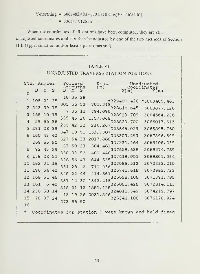
Y-northing = 3063485.483 + [701.318 Cos(303°56'52.6")]

= 3063877.126 m

When the coordinates of all stations have been computed, they are still

unadjusted coordinates and can then be adjusted by one of the two methods of Section

II.E (approximation and/or least squares method).

TABLE VII

UNADJUSTED TRAVERSE STATION POSITIONS

Stn. Angles Forwa]rd Dist. UnadjustedAzimuths (m) Coordmates

D M S D

18

M

35

S

28

X(m) Y(m)

1 105 21 25303 56 53

*329400. 420701. 318

*3063485. 483

2 243 39 187 36 11

328818. 645794. 090

3063877. 126

3 168 10 15355 46 26

328923. 7091357. 068

3064664. 236

4 59 55 56235 42 22

328823. 700216. 267

3066017. 613

5 291 28 29347 10 51

328645. 0291539. 307

3065895. 760

6 160 43 42327 54 33

328303. 4932017. 880

3067396. 699

7 269 55 5057 50 23

327231. 464504. 481

3069106. 259

8 92 43 29330 33 52

327658. 538489. 448

3069374. 789

9 178 22 51328 56 43

327418. 001644. 535

3069801. 054

10 182 31 19331 28 2

327085. 512719. 956

3070353. 210

11 196 54 42348 22 44

326741. 616414. 561

3070985. 723

12 168 51 46337 14 30

326658. 1061542. 415

3071391. 785

13 161 6 42318 21 12

326061. 4281881. 128

3072814. 113

14 236 58 1415 19 26

324811. 3492031. 346

3074219. 797

15 78 37 24273 56 50

325348. 180 3076178. 924

16

* Coordinates for sstation 1 were known and held fixed.

35

D. ADJUSTMENT BY APPROXIMATION METHODIn this thesisTthe method of Compass or Bowditch rule was used to adjusted the

data in Tables III and IV. Thus, the first step is to determine the angular error of

closure and adjust the angles to obtain the proper closing azimuth (closed azimuth at

fixed stations).

1. Angular Errors of Closure

In the closed-connecting traverse, when there are n stations of observed

horizontal angles, n-1 lines will be measured. An angular error in traverse can be

checked and obtained at the last station by comparing the computed azimuth and

closing azimuth at the known station.

The closing azimuth computed (from the known station coordinates at the

traverse end) at the station 15 is 273° 57' 12.0". But because of error in measurement,

the azimuth computed through the traverse at this station is 273° 56' 49.6", which is a

difficiency of 22.4". This amount of angular error in 15 observed stations meets the

limit for allowable error for a third-order class I traverse (allowable error from Table I

is 38.7").

The average correction (Table VIII) is distributed uniformly over all the 15

traverse angles (Table III).

2. Linear Errors of Closure

When all angles have been corrected, the process of calculating the improved

coordinates of all traverse stations may be done. The check on angular closure for a

closed traverse does not guarantee that the entire survey is correct, because there can

be considerable errors in the linear measurement of individual lines. Such errors may

not show up in the angular check. In order to check the closure of the traverse, it is

necessary to determine linear error.

The linear error (LE), the departure error (Sx), and latitude error (dy) in a

traverse are determined by equations

LE = [(6x)2 + (8y)2

]

1 /2(4 .9)

Sx = GEn -GEn (4.10)

36

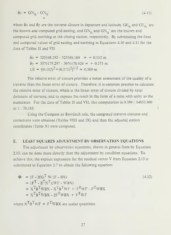
8y= GNn -GNn (4.11)

where 5x and 5y are the traverse closure in departure and latitude, GEn and GEn' are

the known and computed grid easting, and GN and GN ' are the known and

computed grid northing at the closing station, respectively. By substituting the fixed

and computed values of grid easting and northing in Equations 4.10 and 4.1 1 for the

data of Tables II and VII

5x = 325348.292 - 325348.180 = + 0.112 mSy = 3076179.297 - 3076178.924 = + 0.373 mLE = [(0.112)

2 + (0.373)2

]

1'2 = 0.389 m

The relative error of closure provides a better assessment of the quality of a

traverse than the linear error of closure. Therefore, it is common practice to calculate

the relative error of closure, which is the linear error of closure divided by total

distances of traverse, and to express the result in the form of a ratio with unity as the

numerator. For the data of Tables II and VII, this computation is 0.389 / 14853.800

or 1 : 38,185.

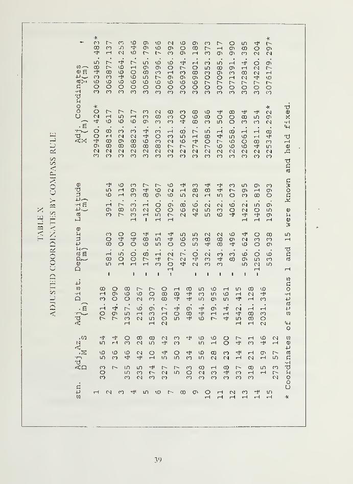
Using the Compass or Bowditch rule, the computed traverse closures and

corrections were obtained (Tables VIII and IX) and then the adjusted station

coordinates (Table X) were computed.

E. LEAST SQUARES ADJUSTMENT BY OBSERVATION EQUATIONS

The adjustment by observation equations, shown in general form by Equation

2.13, can be done more directly than the adjustment by condition equations. To

achieve this, the explicit expression for the residual vector V from Equation 2.13 is

substituted in Equation 2.7 to obtain the following equation:

O = (F - BX)T W (F - BX) (4.12)

= (FT - BTXT)(WF - WBX)

= XTBTWBX - XTBTWF + FT\VF - FTWBX= XTBTWBX - 2FTWBX + FTWF

T T Twhere X B \VF = F WBX are scalar quantities.

37

TABLE VIII

TRAVERSE CLOSURE

I) Angular error

Known azimuth at last station 273 57' 11.95"

Computed azimuth 273° 56' 49.58"Angular error 22. 37Angular correction per station 1. 49

II) Linear error before adjusting azimuths

Known Coordinate X(m) Y(m)at Turtle 2 325348.292 3076179.297

Computed Coordinateat Turtle 2 325348.180 3076178.924Error 6x = + 0. 112 Sy = + 0. 373

Linear error of closure 0. 389 mTotal distances 14853.800 mRelative error of closure 1 / 38,185

TABLE IX

LATITUDE AND DEPARTURE CORRECTIONS

Traverse lines X-correction (m) Y -correction (m)

1 _ 0. 031 + 0. 0072 - 0. 035 + 0. 0083 - 0. 061 + 0. 0124 - 0. 010 + 0. 0025 - 0. 069 + 0. 0156 - 0. 090 + 0. 0197 - 0. 022 + 0. 0058 - 0. 022 + 0. 0059 - 0. 029 + 0. 006

10 - 0. 032 + 0. 00711 - 0. 018 + 0. 00412 - 0. 069 + 0. 01513 - 0. 084 + 0. 01814 0. 090 + 0. 020

38

x K— CO r- CO '£> CT. M0 CM M0 <LT« CO r^- O LO ^ r-CO ro -O <3< CJ> vO tT> o CO t^ H CP> 00 O cn<tf i-i CM M0 f>- r- CO CTi H co cr> cr> CO CM CM

lo r^ «* h- LO M0 M0 <* rH CO LO rH <# o CT>OT^» CO r^ v£> rH CT> cn o r- o LO 00 cr> rH CM t^>o) g ^ CO M0 O CO CO rH CO CO CO 0^ CO 00 CM rHPv— n oo ^ M0 LO c» <_T> a> CT> o o rH CM <# M0ttJ>H MO MO vO M0 M0 M0 M0 M0 M0 r^ I> r^ r~- r^- r-fi o o O O o o o o O o o o o o oH•d

to CO CO CO co CO CO CO CO CO CO CO CO CO CO

* * -do o f- r- r- CO CM 00 co CO M0 <tf CO «* ^ CM a)u CM rH LO rH CO CO CO o M0 CO o o CO LO CT> *

-—< <# M0 v£> M0 CT» CO CO <tf 00 CO LO o CO CO CM -H<H

'1—K_^ O CO CO CO <* CO rH CO r- LO rH ro rH rH COW -d O rH CM 0>1 ^ o CO LO iH CO ^ LO M0 rH H1 TJ—1 <cx ^ 00 Ol CO M0 CO CM M0 ^ o r- M0 O 00 CO rHD <T> CO co CO 00 00 f» I> c-~ r- M0 MO M0 «* LO <Dj%/ CM CM CM CM CM CM CM CM CM CM CM CM CM CM CnI rd

CO CO co co CO CO CO co CO CO co CO CO CO CO00OO

<•d

rdCI,

s COU

a) <* M0 CO t^ r- M0 ^ CO H< ^ co LO cn CO 2"d LO H CTi "* M0 CM rH CO 00 ^ r^ CT> rH cr> O3 M0 rH CO CO m M0 LO CM rH LO o CO CO O C

> 4-><-» Xca •H g rH r^ CO rH o CT« CO MO CM CM M0 CM LO cn

X p— CF> CO LO CM o O M0 CM LO CO o CM o LO CD

tuOO cd CO r^ CO rH LO r-« CM «* LO M0 H1 <* ^ cn U

J rH 1 rH rH rH rH rH (1)

-J r—

'

^CO ^

<u<*

y. u CO o O ^ rH <tf LO LO CM CM M0 * o CO LOH 3 o <* <tf 00 LO ^ M0 CO 00 00 0^ CM CO CO rH

a -p CO o O M0 LO o O LO ^ CO ^ M0 o CT-

^ ^^ T)

oo

K) g rH LO o 00 rH CM r- O CM co CO M0 o MO CCW CO o o r-- *V r-> CM «tf CO <* 00 CT« LO CO rt

d) LO iH rH rH co o <* CM CO CO LO CM LOu Q rH rH rH

a 1 1 1 i 1 1 1 1 1 1 1

Ww P ai—

•

w X 3 cr ) r- r> 3 iH X D JO H JO X JO Obo •H rH CT> l£ > m:) 3 X (n tf "O -O JO H rM * •HD Q ro O C 1 CM •o X •* * -O J> -O ^ H o P—1 —

(TJ

Q • g h ^ r- M0 LTi — * y> * rj> * :m H H -L-'

< •r->^ O CJi LO rH o H (3 X) tf H H ^ X •o in

T> r~- r- co cm -O 3 I-O * JO -«, * -O X 3< rH H N H H M

o

.co * >* c1 CO x IM ("0 * JO JO o r> H j0 CM in

N lO rH ro -O ^ (~o -O H 3 ^ "0 -f rH <D

< P•s kO M0 M0 CM 3 ^ (3 ^ JO X o ^ H T> r^ CCJ

l~l i/) n ^ ^ H -O 1f) ro -O •N N H M H LO a-a •H<Q ro r- io to * > 1

""» -o X H X r- X .o co -do LO CO > M 1-O 3 :m o sf1 ro H h r^ 5-i

CO CO CM ~o ro "0 ro o ro ro ro OJ ooud

p iH CM CO «tf LO M0 r-« 00 CT> o rH CM CO -* LOw rH rH rH rH rH H •K

39

The minimization of Equation 4.12 can be done by taking partial derivative with

respected to each unknown variable (X)

<P = d<D!dX = 2XTBTWB - 2FTWB = (4.13)

Transposing Equation 4.13 and rearranging yields

(BTWB)X = BTWF (4.14)

or

NX + U = (4.15)

T Twhere N = (B WB) is the normal matrix of dimension u by u, and U is B WF. Then

X = -N_1U (4.16)

For the adjustment in traverse, the vector V in equation 2.13 is represented the

residual of observed angles and distances. If there are n observed angles in a traverse,

there will be n - 1 observed distances and the number of residuals becomes 2n+ 1

which includes the residual of angles and distances.

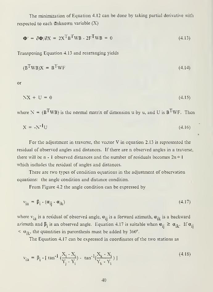
There are two types of condition equations in the adjustment of observation

equations: the angle condition and distance condition.

From Figure 4.2 the angle condition can be expressed by

via = Pi - («ij " « lk > <4 ' 17 )

where vja

is a residual of observed angle, a-: is a forward azimuth, a-^ is a backward

azimuth and 0- is an observed angle. Equation 4.17 is suitable when a- ^ a-^. IF cc-

< a-^, the quantities in parenthesis must be added by 360°.

The Equation 4.17 can be expressed in coordinates of the two stations as

vi

X. -X. 1 X. -X. (4.18)

ia=

Pi-

[ tan"1M—L). tan-lfcJL—i)]

j i

xk '

i

40

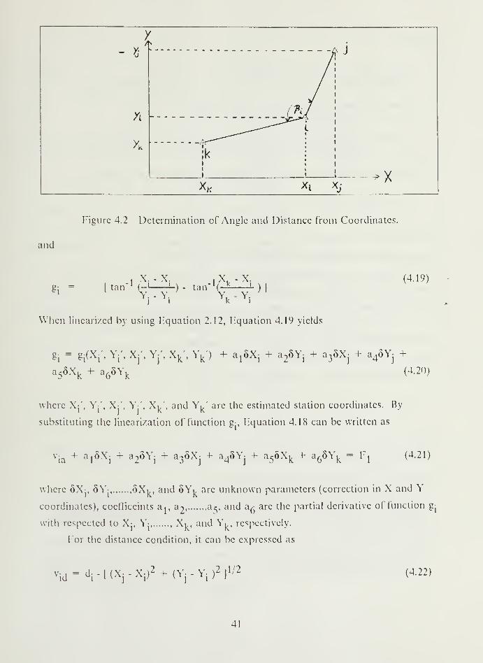
and

Figure 4.2 Determination of Angle and Distance from Coordinates.

, X. - X. , X. - X.tan"

1 H — ) - tan'L

( r

k _' )

(4.19)

] '

Y, - Y,k i

When linearized by using liquation 2.12, liquation 4.19 yields

g; = g:(X:\ Y;', X:', Y;\ Xu' , Yu) + a,5X: + a->5Y: + a,5X: + a45Y: +:

i~ Bi^i- M"V I j»^k« 'k

a56X

k+ a

66Y

k

l

u/h i- ^3«^j - <Mu,

j

(4.20)

where Xj', Y-', X:', Y:', X^', and YR

' arc the estimated station coordinates. By

substituting the linearization of function g:, Equation 4.18 can be written as

via

+ a,5X1

+ a26Yj 4- a

3oXj + a45Yj

+ a56X

R4- a

65Y

R= U

{(4.21)

where 5X-, 6Y- ^XR , an<^ ^\ are unknown parameters (correction in X and Y

coordinates), coefliccints aj, a2

a^, and a^ arc the partial derivative of function gj

with respected to X- Y XR , and Y

R, respectively.

For the distance condition, it can be expressed as

vid

= d[.[(Xr X

[)2 + (Yr Y

[ )2

]

[ l2 (4.22)

41

where

»H- [(Xj

-Xi)2 + (Yj-Yj)2

]

1 / 2 (4.23)

The linerized form of Equation 4.23 is then given as

I4 - hi(Xi', Yi', Xj', Y|', Xk', Yk') + b

{6X

{+ b

26Y

i+ b

36X

j

+ b^Yj (4.24)

Substituting the linearized form from Equation 4.24, Equation 4.22 becomes

vid

+ bjSXj + b25Yj + b

35Xj + b

45Yj = F

2 (4.25)

where Fl and F2 represent the constant form for Equations 4.21 and 4.25. Table XI

shows the partial derivatives for Equations 4.21 and 4.25.

Sometimes, the station positions which is determined by intersection from

traverse station is also to be adjusted simultaneously with traverse station positions.

In this case only the angle conditions are added to observation equations of traverse.

In the data adjusted under this thesis, there are 15 observed angles and 14

oberved distances which consisted of 13 unknown points, consequently, there will be 29

observation equations included 26 parameters of §X and 5Y. Thus, they can be

expressed in matrix form of Equation 2.13 as

V29,l

+ B29,26

X26,1

= F29,l (426)

where Vj j, v2 j,

Vj^jare the residuals of angles; Vj^

j,Vjy

j,v2q j

are the

residuals of distances; B is the coefficeint matrix (consistings of a's and b's) of

parameter X (Table XI); and F is the constant vector.

When three intersection points with 10 observed angles were added (Figure 3.1)

to adjust the coordinates, the observation equations have 39 equations including 32

unknown parameters.

V39,l

+ B39,32

X32,1 = F

39,l <4 - 27 )

42

TABLE XI

THE COEFFICIENTS OF ANGLE AND DISTANCE CONDITIONS

=3-l± =

Yi - Y

i +Yk - Yk

dX± (S^) 2 (Sik )

2

= £ii = +x

i - xi

xk - xkdY

±(s

i:j )

2 (s ik )

2a

^ Y1

- Y±a 7 = = + —> r3 axj (Sij)z

a = 0*1. = .x

i - xi

4 5Yj

(S~~P"

a = -«Hjl =Yk - Y

i5

^xk (s ik>

2

a =d_lL = +

xk " xi

6 ^Yk <slk )

a

5h H X_- - X,bn = —i = + -^ 3,

^Xi

S ij

ah, Y, - Y,bo = —i- = + -> ^

5Yi

S ij

5h H X H- X,

b, = —! = - -J i-

aXj SiJ

dh±=

Yi

- Yi

'1

>2

'3

b4 =

By using Equation 4.16, N is the cofactor matrix and the diagonal terms of this

matrix gives the variances of the adjusted coordinates. To obtain the residuals of all

observed quantities, the reverse process must be done. The correction of X and Y

adjusted coordinates and their standard deviation (cr's) are shown in Table XII. And

the adjusted standard deviation of observed quantities were obtained by multiplying

standard deviation of unit weight [(V WV / r) ' ] to a squares root of diagonal

element of B(BTWB)_1BT matrix (Table XIII).

43

^_^cm r» o 00 O- in rH m CO CM rH CO CO

—

H

CO LT) iH o CO U") yQ yQ vD cn vD rH vD

o o tH rH rH rH rH iH rH o rH rH O

too o o o O O O o o o O o O

to ^ o 00 rH ^ CO rH i£> o CO O -* CM <tf

en «* i> vD rH l> yQ O r^ m 00 m ^ <tf CMCQ «* rH CsJ vD CO t> CO (Ti rH CO co CT> CO rH cn

LT) t-~ -tf t> If) <D vD <# rH CO m rH «* O 0000 o vD tH <T> cn O O- O m 00 cn rH CM i>^ CO vD o CO co rH co 00 co cn CO 00 CM rH

5^ co n ^ vD m i> cn <r> cn o o rH CN <* VD

vd vD ID vD vD vD VD VD ID o t> l> [> l>> O>-( o o O o O O O o o o o o O O oO co CO CO CO CO CO CO CO CO CO co CO CO co CO

7: Oo U

^^.^^ o i> CM <tf CO IT) rH in CM «* <tf CO coH

0)*Hco «* vD vD i> 1^ yQ <D o o o 00 m

< o o o O o rH rH rH rH rH rH o oD -Pw

3to•r—

i

o o o O o O o o o O O o o

O-a o vD CN CO vD o O CM CO CO rH ^ cn co o< CM CO [*- tH <* CO CO O vD r^ cn cn i> t"- 00

<# VD vD vd G> co CO ^ 00 CO <* cn CO co tH

H <*•>

<>

e o CO CO CO ^ CO rH CO l> in rH r- rH rH CO« o tH CNJ CM ^ o CO m rH 00 ^ m vD rH <#

X * CO en CO vD co CM yo <* O l> yQ O CO coen CO CO CO 00 CO i> i> r~- r^ yQ vD vD -* mw CN c\j CM CM CM CM CNJ CM CM CM CM CN CM CM CM

~ 55 co CO co CO CO CO co CO CO CO co CO CO CO COi—c 22

X o

TABLE

TES

BYCO CO ^ m CM LO o rH CM o rH CM rH ^C>i iH CO m LO r- rH rH CM ^ VD l> CO <*

OT) o o o O o iH rH rH rH rH iH CM CO•H4-> o o o O o O O o o O O o OU + + + + + + + + + + + + +

< d)

^ cn t> r- CO CM m yQ 00 co m CM cn <*

^x o CO co 00 rH CO CO co CO CM rH ^ CM

Q OT) oo

oo

oo

oo

rH

OrH

orH

orH

orH

OrH

orH

OoO

OOO 1 1 i 1 1 1 1 1 1 1 1 +

Ou VD ^ co o cn (T> <n <# o CO in co r-

CO CM co i-H vD cn m 00 m rH CM 00 rH cnQ a) tH CM vd l> vD CM r~- o CM r- i> rH t«-

W -P—

>

H «5£ r- <# h- LO vD yQ <* iH co m rH <# cnV) C^- i> vd H in en o i> o in CO cn rH rH

D •H>H CO vd O CO CO rH CO 00 CO cn co CO CM—

i

-a co «* vD LO o- cn cn cn o o rH CM ^Q ^ VD \o <D vD vD yo ID yQ l> o l> l> I>

< O o O o o o o o o o o o oo CO co co CO CO CO CO co CO co co CO couV LO CT> o en CO «* CO rH CM <D ID 00 cn<0 «* O o CM en yQ CO o iH rH o CN *+J— vD t> l> o ^ ^ m o m iD iH <* COcuee~ CO CO co IT) co rH 00 00 in rH 00 rH rH•hX H CM CM «* o CO m rH 00 ^ in vD rH-p co cn CO vD CO CM yQ ^ o r^ ID O COw CO CO CO CO CO l> l> l> t> vD vD VD ^u CM CM CM CM CM CM CM CM CM CM CN CN CM

dp

CO CO CO CO CO CO CO CO CO CO CO CO cn.

O rH CM CO ^ mC/l rH CM co <# IT) vD r- co cn iH rH rH rH rH tH

44

TABLE XIII

ADJUSTED STANDARD DEVIATION OF ANGLES AND DISTANCES

Number Angles Distances

seconds meter

1 W 0. 0292 8. 9 0. 0353 9. 1 0. 0454 9.2 0. 0245 9. 3 0. 0486 9. 4 0. 0567 8. 4 0. 0308 8. 5 0. 0299 7. 8 0. 032

10 7. 1 0. 03411 9. 6 0. 02812 9. 7 0. 04813 9. 8 0. 05414 6. 8 0. 05815 6. 8

45

V. ANALYSIS OF RESULTS

A. COMPARISON OF ADJUSTED COORDINATES

If the given coordinates of the control points are assumed to be error free, then

the accuracy of the traverse station coordinates depends only on the accuracy of

distance and angle measurements. The adjusted traverse coordinates obtained by the

approximation method are of a lower order of accuracy as only the errors in the

misclosure in azimuths and distances were determined. These errors were distributed

by assuming that all observed quantities had an equal probable occurrence.

The least squares adjustment method provides a better approximation of the true

value. Therefore, the adjusted traverse coordinates obtained by this technique provided

better estimates for position of all traverse stations and the accuracy of the adjustment

can be checked and statistically tested.

After the 13 adjusted traverse station (from stations 2 to 14) coordinates

obtained by the approximation method and by the least squares method were

compared, the difference in coordinates at each station were computed and plotted

(Table XIV and Figure 5.1). The largest difference was at station 14. Because stations

1 and 15 are held fixed, the least squares techniques adjusts simultaneously errors in

azimuths and distances, while the adjustment by approximation adjusts errors in

azimuths and distances sequentially. Consequently, the largest difference in traverse

distances occurs at the last station (station 14) before closing of traverse at the fixed

station.

When the standard deviation of observed quantities before the adjustment

(Tables III and IV) were compared with those obtained through adjustment (Table

XIII), the standard deviation of all observed quantities in Table XIII showed

increments. That means, the estimated standard deviations were optimistic.

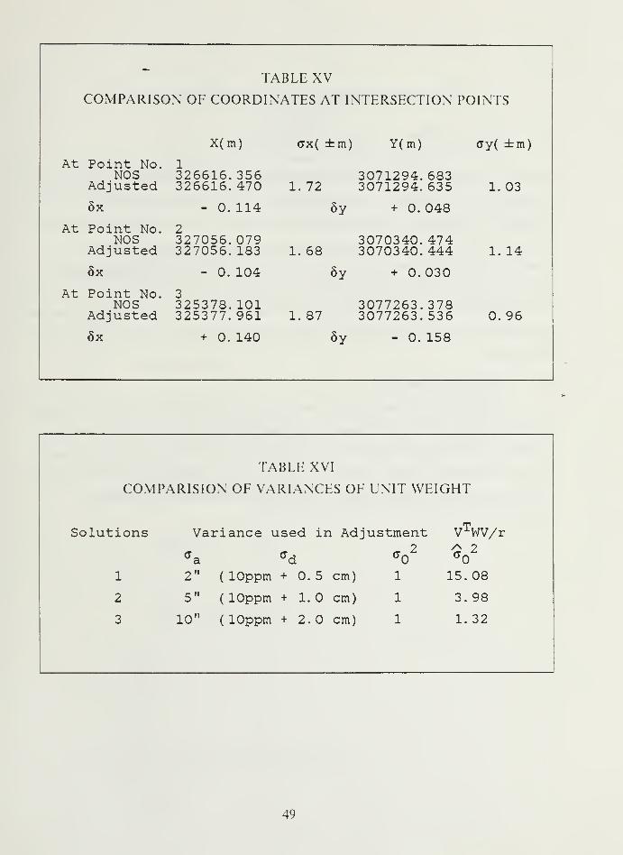
In this thesis, the three intersection points were also adjusted. The adjusted

coordinates of these were compared to NOS results. The largest difference occurs at

point no. 3 (5x = + 0.140 m; Sy = - 0.158 m). The standard deviation of adjusted

coordinates at this point are crx3= ± 1.87, ay

3= ± 0.96 m (Table XV).

46

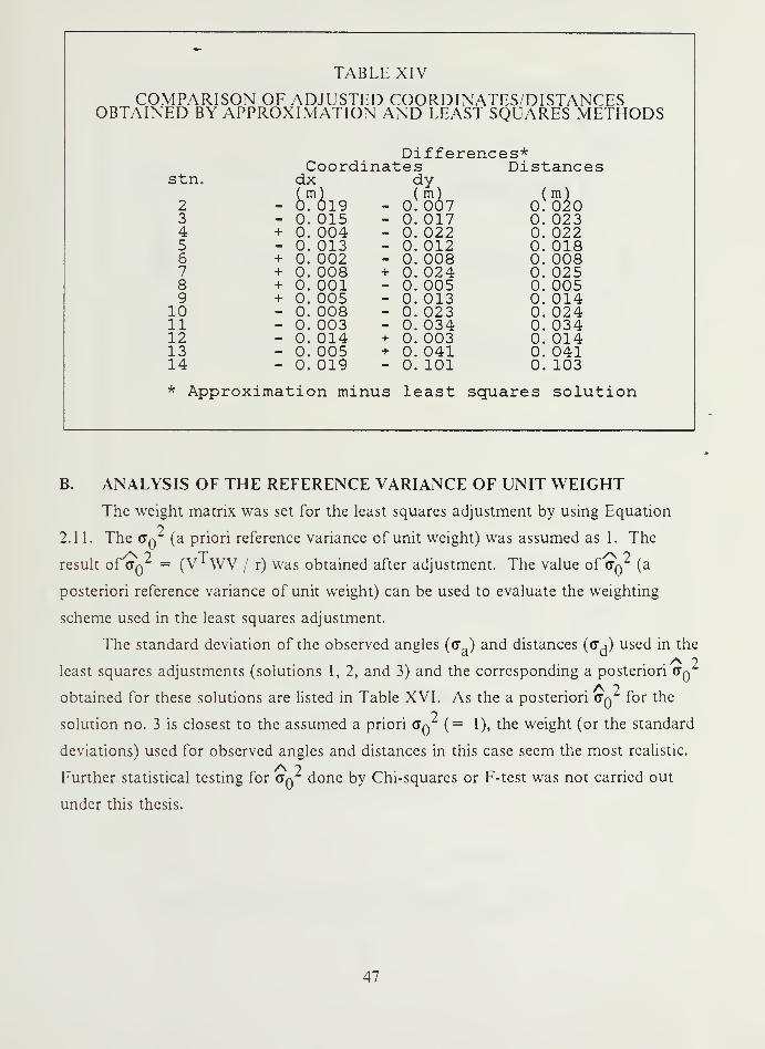
TABLE XIV

COMPARISON OF ADJUSTED COORDINATES/DISTANCESOBTAINED BY APPROXIMATION AND LEAST SQUARES METHODS

Differences*

stn. dx

2 _m0l9

3 - 0. 0154 + 0. 0045 - 0. 0136 + 0. 0027 + 0. 0088 + 0. 0019 + 0. 005

10 - 0. 00811 - 0. 00312 - 0. 01413 - 0. 00514 - 0. 019

a -tes Distances?y*

mm

(m)0. 007

(m)0. 020

- 0. 017 0. 023- 0. 022 0. 022- 0. 012 0. 018- 0. 008 0. 008+ 0. 024 0. 025- 0. 005 0. 005- 0. 013 0. 014- 0. 023 0. 024- 0. 034 0. 034+ 0. 003 0. 014+ 0. 041 0. 041- 0. 101 0. 103

* Approximation minus least squares solution

B. ANALYSIS OF THE REFERENCE VARIANCE OF UNIT WEIGHT

The weight matrix was set for the least squares adjustment by using Equation

2.1 1. The (Tq (a priori reference variance of unit weight) was assumed as 1. The

result of (Tq^ = (VHVV / r) was obtained after adjustment. The value of (Tq (a

posteriori reference variance of unit weight) can be used to evaluate the weighting

scheme used in the least squares adjustment.

The standard deviation of the observed angles ((7a ) and distances (<y^) used in the

least squares adjustments (solutions 1, 2, and 3) and the corresponding a posteriori <Tq

obtained for these solutions are listed in Table XVI. As the a posteriori <Tq for the

solution no. 3 is closest to the assumed a priori Gq (= 1), the weight (or the standard

deviations) used for observed angles and distances in this case seem the most realistic.

Further statistical testing for (Tq^ done by Chi-squares or F-test was not carried out

under this thesis.

47

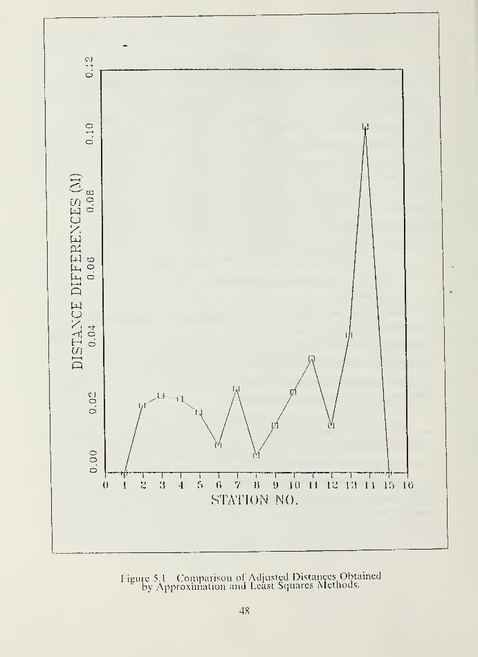
Figure 5.1 Comparison of Adjusted Distances Obtainedby Approximation and Least Squares Methods.

48

-TABLE XV

COMPARISON OF COORDINATES AT INTERSECTION POINTS

X(m) dx( ±m) Y(m) <yy( ±m)

At Point No.NOS

Adjusted

1326616. 356326616. 470 1. 72

3071294. 6833071294. 635 1. 03

Sx - 0. 114 Sy + 0. 048

At Point No.NOS

Adjusted

2327056. 079327056. 183 1. 68

3070340. 4743070340. 444 1. 14

6x - 0. 104 Sy + 0. 030

At Point No.NOS

Adjusted

3325378. 101325377. 961 1. 87

3077263. 3783077263. 536 0. 96

Sx + 0. 140 Sy - 0. 158

TABLE XVI

COMPARISION OF VARIANCES OF UNIT WEIGHT

Solutions Variance used in Adj us tment VTWV/r

*a *d °o2 ^ 2

°0

1 2'*( lOppm + 0. 5 cm) 1 15. 08

2 5" ( lOppm + 1. cm) 1 3. 98

3 10" ( lOppm + 2. cm) 1 1. 32

49

VI. CONCLUSIONS AND RECOMMENDATIONS

A. CONCLUSIONS

By using the weight of observed quantities for the adjustment, the traverse

station coordinates computed and adjusted by the least squares observation equations

method were more accurate than those obtained by the approximation methods. Even

though the observation equations method may require a greater number of equations

than the condition equations method, the processing of the data for adjustment is

easier and the corrections in X and Y coordinates can be directly obtained through

iterative solution. This method is suitable when a computer with a memory capacity of

over 500 K bytes is available. However, for local work or a relatively short traverse, an

approximation method is commonly utilized when economic and logistic criteria are

considered.

B. RECOMMENDATIONThe INDTRA Fortran program written for this thesis is automated for handling

only two kinds of survey techniques: traversing and intersection. With the computers

available at NPS, the development of adjustment programs for covering a wide range

of survey techniques should be done to use and continue analysis of the mixed kind of

survey techniques including traverse, triangulation, trilateration, resection, and

intersection.

50

APPENDIX A

LINEARIZATIONS

This is a linearized form of m functions in n unknowns.

Yl = ^(xp x2 ,..., xn)

y2= f2(Xl ,x2,...,xn)

V = f (x,, Xo,..-, x_)-m m v 1' Z' ' n 7

Y° =y2

°

m

^(Xj , x2

, ..., xn )

2 2 ' 2 ''"' n '

f (x ° X ° ' X u)

yx

dY

ax

gyj gyj_dy,

ax, ax2

axr

ax, ay- ax

AX =

Ax,Ax

2

Ax,

The general form of linearized functions becomes

Y = Y° + J yxAX

51

APPENDIX B

TRAVADJ FORTRAN PROGRAM

This program is used for computing and adjusting the traverse station position by

approximation method (Compass rule).

CCCCCCCCCCCCCCCCCCCCCCCCCCCCCCCCCCCCCCCCCCCCCCCCCCCCCCCc cC FORTRAN PROGRAM "TRAVADJ" Cc cC THIS PROGRAM IS USED FOR CC 1) REDUCE SLOPE DISTANCE TO ELLIPSOIDAL DISTANCE CC 2) DETERMINE GRID DISTANCE CC 3) COMPUTE CLOSE TRAVERSE CC 4) ADJUST COORDINATE BY COMPASS RULE Cc cccccccccccccccccccccccccccccccccccccccccccccccccccccccccccccccccccccccccccccccccccccccccccccccccccccccccccccccccc cC INPUT DATA CC 1) SEMIMAJOR AXIS OF REFERENCE ELLIPSOID USED Cc "a" cC 2) VALUE OF 1/F (EX. 1/F = 294.978698 Cc "f" cC 3) CENTRAL SCALE FACTOR Cc ''ko" cC 4) LAT. AT STARTING AND CLOSING POINT Cc "idl,iml,sl.id2,im2,s2" cC 5) GRID N. AND £. OF 4 ftNOWN STATION Cc "qnl ,qel ,qn2,qe2,qn3 ,qe3 ,qn4,qn4" cC 6) NUHBEft OF MEAGRE DISTANCF. Cc "n" cC 7) ELEVATJON AT FIRST OCCUPIED POINT C

C 8) NAME8OF ALL STATIONS C

C 9) INDICATOR VALUE 1 = NO VERTICAL ANGLE CC 2 = VERTICAL ANGLE CC 10) DIFFERENT IN ELEVATION BETWEEN TWO STATIONS CC 11) SLOPE DISTANCE (WITH UNIT FEET OR METER) Cc "dist" cC 12) HORIZONTAL ANGLES CC CCCCCCCCCCCCCCCCCCCCCCCCCCCCCCCCCCCCCCCCCCCCCCCCCCCCCCCCcccccccccccccccccccccccccccccccccccccccccccccccccccccccccc cc sfac = scale factor coorectionc hgd = horizontal distance cc todis= total distance in traverse cc cegrid = grid east of traverse station cc cnqrid = grid north of traverse station cc difazi = azimuth misclosure cc difdis = distance misclosure cc coraz = angular correction per station ccccccccccccccccccccccccccccccccccccccccccccccccccccccccc cc gridaz = subroutine for computing azimuth c

52

cccccccccccccccccc

utm

dmsr

rdms

between two traverse stations= subroutine for computing the grid"coordinates from known distanceand azimuth

= subroutine for converting the anglefrom degrees, minutes, and seconds toradians

= subroutine for converting the anglefrom radians to degrees, minutes, andseconds

cc

cccccc

c

cc

cccccccccccccccccccccccccccccccccccccccccccccccccc

DIMENSION LAT(3).K(3),HGD(30),HAGL(30,,HANG(30)

DIMENSION NAME3(2),NAME4(5),MDIST(30)DIMENSION DHAGL( 30),NAME(3,30),NAME1(5)

VARIABLE DECLARATION

DOUBLE PRECISION

DOUBLE PRECISION

DOUBLE PRECISION

DOUBLE PRECISION AN90R,AN180R,AN360R.AZC,AZFIR,AZIMUTo AZLAS,CEGRHJ(301,C(JAZR(30l,C0^AZ^CN^RID(30J,DISTAN,DIFAZI,DELTAX(30],DELTAY(30),DUMMY1,DUMMY2,DUMDIS,DIFDIS,T0DIS

NUMO , NUM360 . NUM1 , SUMDX . SUMDY . STDD( 30 ) , STDA( 30)

,

XGD,YGD,NUMf80,Nl)M90,Wto(3J

ANGS(30),CFAZSi(30) j DUM1D,DUM1M,DUM1S,EAZis,EAZ2S,C0RDXl,C0RDYl,TEMS\AZS21,AZS34

sumix1,sumix2,sumfy,sunfx,sumc0y,sumc0x,s$ta,ss^d.sigx\sigy.sigxy'semaj.$emin,SETA, SETAA.SSlfiX.SSiGY.SSiGXY.DEGl, MINI.SECON1,SEMAJ1,SEMIN1,TEMP01(30),TEMP02(30),DDIFFXiDDIFFY

REAL*8 AAC,D,H A R,V,X AY.GD ADH A ZD A CON.CUV A LAT A PHE,CUVRE,ELEVREAL*8 HfJlS^T' SDlS^T A M!!)I^T A ESQft ,GftAMMA. AN6 AAN6V A Pi ,AGU , Fl , F2REAL*8 K,KO.El,E2.0l,Q2,ftR,VV ECEN.FAC.SFAC.HfiDREAL*8 F,CH6D A CSDiST,DDM AHH A HAGL,CHDISt,DG.[iMS.DS ADDANG,MMANGREAL*8 GNl A GN2\GN3,GN4,GEl,6E2 AGE3.GE4 AAZ2i,AZ34.rjIST21,DIST34REAL*8 SI , §2 . Dl . D2 SV , VANG SHA^L , SANG , t)D , MM , SS , HANG , RRRREAL*8 DUM1,6UM2,DUM3 DUM4 XXXX,YYYYREAL*8 IDD1 IMM1 IDD2 IMM2 DVV,MVV,CUVRER,CUVR,CURVRREAL*8 ZINE,K0SE

INTEGER I 1N.ID1.ID2.IM1.IM2.DV,MV.DHAGL.MHAGL,DANG.MANG,UNIT

INTEGER ANGD730] AAN6M(36) A AD\Jl AERR,AZD2i,AZM2i AAZD34,AZM34INTEGER SSHAGLl3d>.CFAZDnO).CFAZM(30J.MtN2,DE62,

EAZ1D , EAZlrt , EAZ2D , EAZ2M , TEMD , TEMM

DATA DUM1/0. 30480061D0/ , DUM2/500000. 0D0/,DUM3/0. 000001D0/DATA DUM4/3600. 0D0/,SIGANG/5. 0D0/.DUM5/0. 000005D0/,DUM6/0. 005D0/DATA TODIS/0. 0D0/,DUM1070. 0000048481368D0/

DATA NUMO/0. 0D0/,NUM360/360. 0D0/.NUM1/1. 0D0/.SUMDX/0. 0D0/,SUMDY/0. 0D0/,NUM180/180. 0D0/,NUM90/90. OdO/

READREADREADREADREADREADREAD

(5,10 AA F,5 15 ID15 15 ID2,5 16 GN1,5,16 GN2,5 16 GN3(5,16 GN4,

,K0IM1.S1IM2.S2GE1,GE2GE3,GE4

53

READ(5,11)N,ELEV

CALL GRIDAZ (GE1 ,GN1,GE2,GN2,AZ21 ,DIST21)CALL GRIDAZ (GE3;GN3;GE4,GN4,AZ34,DIST34)

IDD1 = FLOAT(IDl)IMM1 = FLOATf IM1)

CALL DMSR (IDD1 . IMM1 ,Sl ,D1)LATfl) =6lIDD2 = FLOAT(ID2)IMM2 = FLOATf IM2]

CALL DMSR (IDD2, IMM2,S2,D2)LAT(2) =02

LAT[3) = (Dl+D2)/2.0D0ESQR =iQR = 2.0D0*(l.0D0/FJ-(1.0D0/F)**2

X = A*DSQRTf 1. ODO-ESQR)Y = 1.0D0-(ESQR*(DSIN(LAT(3)))**2)K — X/

Y

CcC DETERMINATION OF THE SCALE FACTOR FOR UTM.CCC

El = DABS(DUM2-GE2)E2 = DABS(DUM2-GE3)

CECEN = ESQR/(1. ODO-ESQR)

c01 = DUM3*E102 = DUM3*E2QPRIME = ((Q1**2)+(Q1*Q2)+(Q2**2))/3.0D0

cDOl M=l,3

RR=A/(1.0D0-ESQR*(DSIN(LAT(M)))**2)**0. 5

Fl = fl.0D0+ECEN*DC0S(LAT(M)))*(10.0D0**12)F2 = 2.0D0*(RR**2)*(KO**2)FAC= F1/F2

CC

KfMj)=KO*(l. ODO+FAC*QPRIME+(0. 00003D0*(QPRIME**2)))

SFAC = K(3)C SFAC = 6. ODO/( ( 1. 0D0/K( 1 ) )+( 4. 0D0/K(3))+(1. 0D0/K(2)))

C

c

READ(5,20) UNIT-'MrREAD(5,18)(NAME1(L),L=1,5)

C DETERMINATION OF THE HORIZONTAL DISTANCESC

DO 1000 J=1,N

READ(5,14)(NAME(L,J),L=1,3)READf5 12jI.DH.DV MV SVREAD[5,13) ^DI^TMDIST(J) = SDIST

CC IN CASE OF THE LENGTH'S UNIT IS IN FEET, THEN CONVERSE TO METER

IF(UNIT. EQ. 1) THENSDIST = SDIST*DUM1

54

DH = DH*DUM1ELEV = ELEV*DUM1

END 4FC

READ(5,17)DHAGL(J),MHAGL(J),SHAGL(J)DD = DFLOATfDHAGLfJ))MM = DFLOATfMHAGL(J))SS = SHAGL(J)

CALL DMSR ( DD,MM^SS,RRR )

HANG(J) = R&RSTDA(J) = SIGANG

CccC DETERMINATION OF HORIZONTAL DISTANCES WHEN THE DIFFERENT INC ELEVATION IS APPROXIMATELY KNOWN.C

IF(I.EQ.1)THEN

IFCDH.NE. O.OJTHENDDM = SDISTIFCDDM.GE. 3300.0)THEN

DO 100 KK=1,3

CURV =(0.016192D0*DDM)CALL DMSR (NUM0,NUM0.CURV,CURVR)D=DSQRT(DDM**2-(DH*D£0S(CURVR)r*2)-DH*DSIN(CURVR)

C100 CONTINUE

CHDIST = DDM

ELSEHDIST = DSQRT(DDM**2-DH**2)

END IF

ELSE

HDIST = SDISTEND IF

END IFCC DETERMINATION OF HORIZONTAL DISTANCE WHEN ZENITH DISTANCE IS KNOWNC

IF(I.EQ. 2)THEN

DVV = FLOAT(DV)MVV = FLOAT(MV)CALL DMSR (DVV'MVV,SV,VANG)CALL DMSR (NUM§0 a NUM0'NUM0'AN90R)CALL DMSR (NUM180\NUM6,NUMO\AN180R)ZD = ANQOR^VANGDH = SDIST^DSINCZD'ds = sdist*dcos(zd;IFf SDIST. GE. 3300.01 THEN

CUVRE = 0. 013925TJ0*SDISTCUV = 0.016192D0*SDISTCALL DMSR (NUM0,NUM0,CUVRE,CUVRER)CALL DMSR (NUMO'NUMO CUV.CUVR)PHE = (AN90R-ZD)+CUVRERC = (AN90R+CUVR)GRAMMA = AN180R-(C+PHE]HDIST = (SDIST*DSIN(GRAMMA))/DSIN(C)

ELSEHDIST = DS

END IFEND IF

55

HH= (ELEV+DH)CC DETERMINATION OF THE HORIZONTAL DISTANCE ON GEOIDC

GD = R*HDIST/(R+H)CC DETERMINATION OF THE GRID DISTANCES

HGD(J) = GD*SFAC

TODIS = TODIS+HGDfJ)STDD(J) = HGD(J)*DUM5+DUM6

WRITE(6,*) 'GRID DISTANCE =' ,HGD(J)WRITE(6;*)' Y

ELEV = HH

1000 CONTINUE

READ(5,19)(NAME3(L),L=1,2),DANG,MANG,SANGREAD(5;18)(NAME4(L);L=1;5)

CALL 0UTPUT(N,AZ21.AZ34.GN2,GE2,GN3.GE3,HGD,DHAGL,MHAGL,SHAGL,*DANG.MANG,SANd > NAM^l.NAME3,^AME4,NAME,MdlST,GNl,G^l,GN4,GE4)

dDANG = DFLOAT(DXNG)MMANG = DFLOAT(MANG)CALL DMSR (DDANG, MMANG, SANG, RRR )

NN = N+lHANG(NN) = RRRSTDA(NN) = SIGANG

CALL DMSR ( NUM360,NUM0,NUM0,AN360R )CALL DMSR ( NUM180,NUM0,NUM0,AN180R )

DO 2000 ADJ1 = 1,2XGD = GE2YGD = GN2AZFIR = AZ21

DO 200 I = 1,NAZIMUT = AZFIR+HANG(I)

IF (AZIMUT. GE.AN360R) THENAZIMUT = AZIMUT-AN360R

END IFIF(AZIMUT.GE.AN180R) THEN

AZIMUT = AZIMUT-AM80RELSE

AZIMUT = AZIMUT+AN180REND IF

COAZR(I) = AZIMUT

CALL RDMS ( AZIMUT,DUM1D,DUM1M,DUM1S )

CFAZD(I) = l6lNT(DClMlD)CFAZM(I) = IDINT(DUMIM)CFAZS(I) = DUM1S

DISTAN = HGD(I)CALL UTM ( XGD, YGD, DISTAN, AZIMUT, DUMMY1 ,DUMMY2 )

WRITE(6,*)'I =' ,1

56

200

230

WRITE(6,*)'GRID E='DELTAXd'

.DUMMYI '

.= DUMMYl-XGd

DELTAYf Ii = DUMMY2-YGDWRITE(6 *i'DEPARTure ='

+DELTAX(I),ZlNE = DSIN(AZIMUt)

KOSE = DCOS(AZIMUT)

GRID N=',DUMMY2

LATITUde =',DELTAY(I)

= SUMQX+DE|_IAX( nSUMDXSUMDY = SUMDY+DELTAY(ICEGRID(I) = DUMMYICNGRID(I) = DUMMY2

CALL GRIDAZ ( XGD, YGD, DUMMYI, DUMMY2,AZC,DUMDIS )

CALL ROMS ( AZC,DUM1D,DUM1M,DUM1S )CBAZD(I) = IDINTfDUMID*CBAZM(I) = IDINT(DUM1M'CBAZS(I) = DUM1S

IF THEN(ADJ1.EQ. 1

TEMPOKITEMP02(I) = CNGRID

END IF

Dm

AZFIR = AZCXGD = DUMMYIYGD = DUMMY2

CONTINUE

IF (ADJ1.NE. 1) THEN

CORDX1 = ( SUMDX-(GE3-GE2) )/TODISCORDY1 = f SUMDY-(GN3-GN2) )/TODISXGD = GE2YGD = GN2

DO 230 1=1,

N

DISTAN = HGD(I)

XXXX = C0RDX1*HGD(I)YYYY = CORDYl*HGDm

DELTAX(I) = DELTAX(I) - XXXXDELTAY(I) = DELTAY(I) - YYYY

CEGRID(I)CNGRID(I)DDIFFXDDIFFY

XGD+ DELTAX(IYGD+ DELTAYfTCEGRIDfl)-TEMPOl(I)CNGRIDC I )-TEMP02( I

)

XGDYGD

CONTINUE

= CEGRIDtn= CNGRID(I

END IFAZLAS = AZFIR+HANG(NN)

IF ( AZLAS. GE.AN360R ) THENAZLAS = AZLAS-AN360R

END IF

IF (AZLAS. GT.AN180R) THEN

57

AZLAS = AZLAS-AN180RELSE

AZLAS = AZLAS+AN180REND IF

CCALL RDMS ( AZLAS,DUM1D,DUM1M,DUM1S )

TEMD = IDINt(DUMlD)TEMM = IDINT(DUMIM)TEMS = DUM1S

CC

DIFAZI = AZLAS-AZ34WPRED(l) = DIFAZICORAZ = DIFAZI/DFLOAT(NN)

CALL RDMS ( DIFAZI. DUM1D.DUM1M.DUM1S )EAZ1D = IDINt(DABS(DUMlD))EAZ1M = IDINTfDABS(DUMlM))EAZ1S = DABS(DUMIS)

CALL RDMS ( CORAZ ,DUM1D.DUM1M,DUM1S )

EAZ2D = IDINT(DAB$(DUM1D))EAZ2M = IDINT[DABS(DUM1M))EAZ2S = DABS(DUMIS)

IF(ADJ1.EQ. 1)THENWPRED(2) = SUMDX -

( GE3-GE2 )

WPREDC3) = SUMDY - f GN3-GN2 )DIFDIS = DSQRT( WPRED(2)**2 + WPRED(3)**2 )ERR = IDINTC TODIS / DIFDIS )

END IFCCC PRINT RESULTS OF TRAVERSE COMPUTATIONCC

CALL RDMS (AZ21.DUM1D.DUM1M.DUM1S)AZD21 = iDINTffiUMID)AZM21 = IDINT(DUMIM)AZS21 = DUM1S

CALL RDMS (AZ34.DUM1D.DUM1M.DUM1S)AZD34 = iDINTfDUMID)AZM34 = IDINT(DUMIM)AZS34 = DUM1S

IF (ADJ1.EQ. 1) THENWRITE(8,29)WRITE(8 27WRITE(8,30'WRITE(8 31"

ELSEWRITE(8,28'WRITE(8 27'

WRITE(8 30"

WRITE(8 40END IFWRITE(8,32'WRITE(8,33'WRITEC8 30"

WRITE(8,34) AZD21,AZM21,AZS21WRITE(8;35) GE2.GN2

DO 240 1=1,

N

II = 1+1CALL RDMS[HANG(I),DUM1D,DUM1M,DUM1S)

ANGD(I) = IDINT(DUMID)ANGMflj = IDINT(DUMIM)ANGSfl) = DUM1SSSHAGL(I) = IDINT(SHAGL(I))

58

c

IF (ADJ1.EQ. 1) THENWlTE(8.3^^

WI^^I

fcg^L(I).CFAZD(I).

WRITE(8,37^ANGDn) ANGMri),ANGS(I),CFAZD(I),CFAZM(I),

END IF^

WRITE(8,38) II,CEGRID(I),CNGRID(I)240 CONTINUE

CALL RDMS ( HANG(NN) ,DUM1D,DUM1M,DUM1S)IF (ADJ1.EQ. 1) THEIsl

DHAGL(NN) = DANGMHAGL(NN) = MANGSSHAGL(NN) = IDINT(SANG)

WRITE(8,36)DHAGL(NN),MHAGL(NN),SSHAGL(NN),TEMD,TEMM,TEMS

CALL RDMS (HANG(NN).DUM1D,DUM1M,DUM1S)ANGD(NN) = IDINT(DUMID)ANGMfNN) = IDINT(DUMIM)ANGD(NN) = IDlNKDUMip

ITE(END IF

ANGS(NN) = DUM1SWRITE(8,37)ANGD(NN) ,ANGM(NN) ,ANGS(NN) ,TEMD,TEMM,TEMS

WRITE(8,30)-1)WRITE(8,39)AZD34,AZM34,AZS34,GE3,GN3

WRITEC8 *) 'V

IF (ADJl.EQ. 1J THENWRITE(8,4I)EAZ1D,EAZ1M,EAZ1SWRITEf 8 , 42 1 EAZ2D , EAZ2M , EAZ2SWRITEC8 43JT0DISWRITEC8 44]DIFDISWRITE(8,45) ERR

END IFCC CORRECTED OBSERVED ANGLESC

c

DO 250 1=1, NNHANG(I) = HANG(I)-CORAZ

250 CONTINUE

SUMDX = O.ODOSUMDY = O.ODO

CC2000 CONTINUE

C

SUMDX = GE3-CEGRID(N)SUMDY = GN3-CNGRIDCN)DIFDIS= DSQRT ( SUMDX**2 + SUMDY**2 )

EAZ1D.EAZ1M.EAZ1SWRITE(8,41) EAZ1D.WRITE(8,44) DIFDI$

10 FORMAT(5X,F15. 5 4 5X^F15, 10, 15X.F12. 8)11 F0RMAT(26X,I4,3^X,F7.3)12 F0RMAT(20X II !4X,F9. 3, 11X,2I3, F10. 4)13 F0RMAT(25X'F15\ 6)14 F0RMAT(6X,3A4)15 F0RMAT(5X,2I3'f14. 8)16 FORMATflO^.FlS. 5,15X^15. 5)17 FCRMAT(25X,2I3,Fl0.4)18 FORMAT? 5A4)19 FORMAT(2A4,17X,2I3,F10. 4)20 FORMAT(H)

C27 FORMAT( 16X ,':::::::::::::::::::::::::::::' ,///)

59

282930

31

40

32

33

343536

37

38C39C41CC42CC43C44C45

F0RMAT(16X,' ADJUSTED TRAVERSE COMPUTATION')

,

x

F0RMATQ5X 'UNADJUSTED TRAVERSE COMPUTATION')FORMAT( r --* i \

STNFORMAT

(

FORMAT

(

*TE(M1FORMAT

(

)

TN

0.FORMAT(*NORTHFORMAT( '

I

FORMATf'I 1.

F0RMAT('I',3X,'

F6RMATC 'I' ,3X,

'

*25X ' I '

)

FORMATfl' 13 '

^KNdWN

OBSERVED

CORR. OBS.

HOR. ANG.

D M S

FORWARD

FORWARD

AZIMUTHS

D M S

,13X,I3,1X,I2,1X.F5.2,34X

GRID

GRID

DIST.

(M.)

I')

COORDINATE (M

ADJUSTED COORDINA

GRID EAST : GRID

'36X:Fl6.3!lX!Fli.3'lVlhY ,i3,lX,i2,iX,I2,4x,i3,lX,I2,lX,F5.2,lX,F8. 3.25X

',13, IX, 12, IX, F5. 2, IX, 13, IX, 12, IX, F5. 2, IX, F8. 3,

36X,F10.3,1X,F11.3,1X,T)2,11X,dATA p ,7X;iJ,l)(,I2!l)(.Fl2,ilX,F10. 3,1X,F11.3,//)

ANGULAR ERROR = f ,2x, 13, IX, 'D' , IX, 12, IX, 'M' , IX, F5.

FORMATflX,FORMATfW 1 '

*2 IX S ' )

FdRMAjr; ANGULAR CORR./ STATION =' ,2X, 13, IX, 'D' , IX, 12, IX, 'M' , IX, F5.*2f6rmAtFORMATFORMATSTOPEND

'TOTAL DISTANCES'LINEAR ERROR'LINEAR CLOSURE

3}= 2X F10.3)= ;3x;'i /r ,i6,///////////)

CCCCCCCCCCCCCCCCCCCCCCCCCCCCCCCCCCCCCCCCCCCCCCCCCCCCCCCCCCCCCCc cC SUBROUTINE TO CALCULATE GRID AZIMUTH AND DISTANCE BETWEEN CC TWO KNOWN STATIONS WITH THEIRS GRID NORTH AND GRID EAST. Cc cccccccccccccccccccccccccccccccccccccccccccccccccccccccccccccccc

SUBROUTINE GRIDAZ (X1,Y1,X2,Y2,ANGLR,DIST12)

cREAL*8 X1.X2.Y1,Y2.ANGLR.ANG0,ANG90,ANG180,ANG270,DIFX,DIFY,DIST12REAL*8 ANG90ft,AN180R,AN270R

DATA ANGO/0. 0D0/.ANG90/90. 0D0/,ANG180/180. 0D0/,ANG270/270. ODO/

ANG90,ANG0.ANG0 AANG90R )

ANG186,ANG6,ANG0,AN180R )ANG270,ANG0,ANG0,AN270R )

CALL DMSRCALL DMSRCALL DMSR

DIFX = X2-X1DIFY = Y2-Y1

IF((DIFX. EQ. ANGO). AND. (DIFY. EQ. ANGO)) THENANGLR = ANGO

ELSE IFf DIFX. EQ. ANGO) THENIF(DIFY.GT.ANGO) THEN

ANGLR = ANGOEND IF

ANGLR = AN180RELSE

IF(DIFX.GT.ANGOJ THENANGLR = ANG90T<-DATAN(DIFY/DIFX)

ELSEv '

ANGLR = AN270R-DATAN(DIFY/DIFX)END IF

END IF

DIST12 = DSQRT(DIFX**2+DIFY**2)

60

RETURNEND

(3(3(3(3(3(3(3(3(9(3(3(3(3(3(3(3(3(3(3(3(3(3(^

(3

(3 SUBROUTINE OUTPUT TO PRINT OUT THE RESULT FOR USING IN (3

(3 THE NEXT COMPUTATION. (3

(3 (3

(3(3(3(3(3(3(3(3(9(3(3(30(3(3(3(3(3(9(3(30^

SUBROUTINE OUTPUT(N.A.B.G2.E2.G3.E3,RD,DH,MH,SH,DA,MA,SA,NAMEl,*NAME3 , NAME4 , NAME , MDfSf ,(h , £l , Gl4 , £4)

10

DIMENSION RD(N),DH(N),MH(N),SH(N),NAME(3,N),NAME1(5),NAME3(,NAME4(5),MDlSTfN)REAL*8 Al6.DG,G2 AG3AE2.E3.RD.AA.BB,HH.SH,SA,SSA,SIGA,SIGDREAL*8 MDI$T,MDIS\RRD,Gl,G4,F.l,£4,DUMiINTEGER N,DH,MH,DA,MA

DATA SIGA/5. 0D0/,DUMl/0. 30480061D0/

2)

WRITE(7WRITE(7WRITE(7WRITE(7WRITE(7WRITE(7WRITE(WRITE!WRITE!WRITE!WRITE!WRITEWRITE(WRITE!WRITE!WRITE!

WRITEWRITEWRITEWRITEWRITEWRITEWRITEWRITEWRITEWRITEWRITE

7

7

777

7

7

7

7

,240'250',260'250'270'280'290'280'240'280'300',310'310'300',280'240'

NAME1(L),L=1.5).G1.E1'NAME(Ll5,L=i.3).G2.E2NAME3(L),L=1,3),G3,£3NAME4(L) L=1,5),G4,E4

(6 230)6 100)6 110)6 120)6 110)6 125)6 140)6 130)U 140)(6 100)(6 140)

Nl = N+l

WRlfEC'6,150)(NAME(L,I-l),L=l,2),(NAME(L,I),L=l,2),DH(I-l),MH(r* l).SH(l-l)

WRITE(6,150)(NAMEfL,N),L=1.2)XNAME3(L),L=1.2).DHfN).MH(N) >SH(N)

WRITE 6 150 (NAME3(L) L=l ,2) ,(NAME4(L L=l,2) DA, MA $AWRITE(6 140)WRITE(6,100)

WRITE(6,230)WRITE(9;i70)

61

20

CC40

100

110

120

125

130

140

150

170

180

190

200

210

220

230240

250

260

270

280

290

300310

WRITEWRITEWRITEWRITEWRITEWRITEWRITEWRITEWRITE

(9 180)9 490)9 180)9 170)9 200)9 210)9 200)9 170)9 200)

DO 20 J=1,N-1mdis = md:RRD = RD(J)MDIS = MDISTf J)*DUM1

7D0M1SIGD = (RD(J)*0.00001D0)+0.01D0WRITE(9 220)(nAME(L

)J),L=1,2),(NAME(L,J+1),L=1,2),MDIS,

MDIST(b) RD(5)SRRD

V

CONTINUEMDIS = MDIST(N)*DUM1RRD = RDCNVDOMlWRITE(9,220)(NAME(L,N),L=1,2),(NAME3(L),L=1,2),MDIS,MDIST(N)

* RD(N)\tfRDSIGD = (RD(N)*0.00001D0)+0.01D0WRITE(9,200rWRITE(9,170:

F0RMAT(2I3,F6.2)FORMAT ( 9X ******************

F0RMAT£9X,'*

AT TO

*************** **************** *******

* * *

FORMATJ^X,'* MEASURED HORIZONTAL ANGLE * * *%

F0RMAT(9X '******************************* DEGREES * MINUTES * SEC*ONDS ™yFORMAT£?X,'*

FORMAT^X, 1 *

F0RMAT(9x\ , *\3Xf2A4,3X, , *',3X,2A4,3X, , * , ,3X,I3,3X, , * , ,4X,I2,3X,

*'*' .2X.FS. 2,5X, '*•

)

*########to#### (

)

F0RMAT(5X,'# # ##')

F0RMAT(5X '# DISTANCES # MEASURED DISTANCES # REDUCE*D DISTANCES #r )

F0RMAT(5X/# # # # #* # # )

F0RMAT(5X '# FROM # TO # METERS § FEET # METERS* # FE£T #Y )F0RMAT(5X . '#' ,2A4; '#' . 2A4 ,'#\2X,F8. 3,2X, '#' ,2X,F8. 2,2X,'# I

,2X,*F8.3.1X ,'r ,2XF8\2,2X,'£')FORMAt('i')FDRMATiQX *******************************************************

F0RMAT(9X,

F0RMAT(9X,

F0RMAT(9X,

FORMAT(9X,

F0RMAT(9X,* \

NAME

OF

KNOWN POSITIONS

* *

COORDINATES

*********************************

* * *

* GRID NORTH * nDTn CACT *GRID EAST

F6RMAT(9X,'*',5A4 '*' .2X.F11.3.2X '*' .2X.F11. 3,2X. '*'

}

FORMAThx, 1 *' 4X,5A4,4x, ut ,2X Fli. 3,2X, '*' ,2X Fll. 3,2X, '*'

)

RETURN

62

ENDCCC 0000000000000000000000000000000000CC CONVERT DEGREES, MINUTES,C (3 AND SECONDS TO ftADIANS (3

C (3

C 0(3(3(3(3(3(3(3(3(3(3(3(3(3(30(3(3(3(3(3(3(300(3(3(3(3(3(3(3(30

Cc

SUBROUTINE DMSR ( D1,M1,S1,R1 )

REAL*8 D1,M1,S1,R1,PI1,N60,N3600,N180

DATA N60/60. 0D0/,N3600/3600. 0D0/,N180/180. ODO/

PI1 = 4. ODO*DATAN(1.0DO)Rl = ((D1+(M1/N60)+(S1/N3600))*PI1)/N180

RETURNEND

CCC 000000000000000000000000000000000CC COMPUTE THE COORDINATESC FROM ONE KNOWN POINT WITHC MEASURED DISTANCE AND ANGLECC 000000000000000000000000000000000C

SUBROUTINE UTM (XI , Yl ,DIS12 , ANG12R , X2 , Y2 )

REAL*8 X1,Y1,X2,Y2,DIS12,ANG12R,DIFX,DIFY

DIFX = DIS12*(DSIN(ANG12R))DIFY = DIS12*(DCOS(ANG12R))X2 = Xl+DIFXY2 = Yl+DIFY

CRETURNEND

CC 000000000000000000000000000000000CC CONVERT ANGLE FROM RADIANC TO DEGREE, MINUTES, SECONDSCC 000000000000000000000000000000000C

SUBROUTINE RDMS ( RR1,D2,M2,S2 )

IREAL-8 RRl.M ,M2.$2.PIl.H60.H180.TOEQ.DIF.™iH

DATA N60/60.0D0/,N180/180.0D0/C

PI1 = 4. ODO*DATANf 1. ODO)TDEG= fN180*RRl)/PllD2 = DFLOATflDINT(TDEG))DIF = TDEG-D2TMIN= DIF*N60M2 = DFLOATflDINT(TMIN))DIF = TMIN-M2S2 = DIF*N60

RETURNEND

63

APPENDIX C

INDTRA FORTRAN PROGRAM

INDTRA Fortran program is used for computing and adjusting traverse station

position by least squares method of observation equations (indirect observation) and

simultaneously adjust the intersection points which are observed at each traverse

station.

C (3(3(3(3(9(3(3(3(3(3(3(3(3(3(3(3(3(3(3(3(3(3(3(90^

C (3(3 (3(3

C (3(3 LEAST SQUARE ADJUSTMENT OF (3(3

C (3(3 OBSERVATION EQUATIONS METHOD (3(3

C (3(3 (3(3

C 0P(3(3(3(3(B(3(3(3(3(3(3|B(3(3(3(3(3(3(3(3(3(cl(3(B(3(3(3(3(30(3(3P(300@

ccC (3(3(3(3(3(3(3(3(3(3(3(3(3(3(3(3(3(3(3(3(3(3(3(3^^

C (3

C (3 N.NA = NUMBER OF OBS. ANGLES (3

C (3 Nftl = NUMBER OF RESECTION PT. (3

C (3 ND = OBS. DISTANCES (3

C (3 NT = OBS. DIST + OBS. ANG. (3

C (3 NC = TRAV. STN. + RESECT. PT, (3

C (3 (NOT INCLUDE KNOWN STN.) (3

C (3 NZ1 = NUMBER OF RESECT. ANGLE AT EACH TRAV. STN. (3

C (3 EGRID = GRID EAST OF KNOWN POINT (3

C (3 NGRID = GRID NORTH OF KNOWN POINT (3

C (3 D.M.S = READ ANGLE IN DEGREES, MINUTES, SECONDS (3

C (3 RANG, DIST = GRID DISTANCES (3

C (3 NCO.ECO = GRID NORTH AND EAST OF INTERSECTION PT. (3

C (3 STDA = STANDARD DEVIATION OF ANG. (3

C (3 STDD = STANDARD DEVIATION OF DIST. (3

C (3 NP2 = NUMBER OF UNKNOWN DX A DY (3

C (3 CEGRID,CNGRID = TRAV. STN. C(!)ORDI. (3

C (3 INDLSQ = SUBROUTINE ADJUSTING THE COORDINATES (3

C (3 BY OBSERVATION EQUATIONS (3

C P CALFM = SUBROUTINE FOR COMPUTING CONSTANT VECTOR (3

C (3 CALAM = SUBROUTINE FOR COMPUTING THE COEFFICIENTS (3

C P OF UNKNOWN PARAMETERS (3

C (3 (3

C (3(3(3(3(3(3(3(3(3(3(3(3(3(3(3(3(3(3(3(3(3(3^^

CCc

DOUBLE PRECISION NGRID(4) .EGRID(4J .AZ21 .DIST21 ,AZ34,* DIST34 , XdD , YGD^AZf^I R . NIJM360.NL)M0

.

AN360R A DD AMM A S$\R AANGlf 40) JTDA[40)

.

DUM10 a R^NG\d1ST(46),NC0,EC0a CNGRID(40),CEGRID(40) A STDD(40),AZIMUT ADIS(40KCOAZR(4O),0UMMYl.DUl5|MY2.AZCACFAZS[4O) >

DOUBLE PRECISION SUMDX ,SUMDY' CBAZSi40) ,TTCOX(40KTTCOYjf 40)

,

AZLAS.DIFAZf.WPREDfSKEAZlS'CORAZ.DIFDIS,EAZ2S,TODIS,ASNY(40),ASEX(46),DUMil,DUM12

DOUBLE PRECISION WM( 80.80J.STDO(80J .FMf 80 ) .BMf 80^80 ) .

BMt(8d.80j,BMTWM(8d,80).Nrt(80.8d),TM(80),DELTA(§0),NMI(80,80),WKi0(428§),VM(l,80),

64

*

stdad,xcox(80),ycoy(80)

integer nt.na,np.np2.nd,ni,pn.asp,printd.n.nsta.d.M a s.cfXzd(4o).cfAzm(40):cbazd(4oj,k,ki(,K4

,

£bAZM( 40) , EAZ1D . EAZ1M; FJ\Z2D , EAZ2M 4 N2

,

NUM(40),ERR,NRl,NZi(40),K10,KON,II,lll,NC

DATA NUM360/360. ODO/,NUMO/0. 0D0ADUM10/2. ODO/DATA DUMll/O. 00001D0/.DUM12/0. 0260/,SUMDX/0. ODO/DATA SUMDY/O. ODO/, TODlS/O. ODO/

CDATA PW/O/.PRINTD/l/

C(3(3 PW = 1 UNWEIGHTC(3(3 PRINTD = NOT PRINT DETAILS OF MATRIXCCC DETERMINE BACK AZIMUT AT STARTING STATION AND FORWARDC AZIMUTH AT CLOSING STATIONCC

DO 1 1=1.4READ(5,*) NGRID(I)READ(5 *) EGRID(I)

1 CONTINUEC

CALL GRIDAZ (EGRID(2) ,NGRID(2) ,EGRID( 1) ,NGRID(1) ,AZ21 ,DIST21)CALL GRIDAZ (EGRID(3) ,NGRID(3) ,EGRID(4) ,NGRID(4) ,AZ34,DIST34)

CCOMPUTE APPROXIMATED COORDINATE OF TRAVERSE STATION POSITIONS

CCC@(3(3 READ NUMBER OF OBSERVED ANGLESC

READ(5,*) N

03(3(3(3 READ NUMBER OF RESECTION POINTC

READ(5,*) NR1

CNSTA = N-lXGD = EGRID(2)YGD = NGRID(2)AZFIR = AZ21

CALL DMSR (NUM360,NUM0,NUM0,AN360R)

K =

C

C

CDO 100 1=1, NSTA

C READ ANGLE IN DEGREE, MINUTE, SECONDREAD(5, 105J D.M.S

Dti = DFLdAf(D)MM = DFLOAT(M)SS = DFLOATfSJ

CALL DMSR (DD,MM,SS,R)

ANG1(I) = RSTDACI) = DUM10

C READ REDUCE GRID DISTANCESREAD(5.M RANG

DfST(I) = RANG

65

READ(5,*) NZ1(I)CC

IF (RANG. EQ. 0.0) THEN

C READ APPROX. GRID COORDINATES OF RESECTION STATIONREAD(5,*) NCOREAD(5,*) ECO

CCNGRID(I) = NCOCEGRID(I) = ECOGO TO 100

END IFC

K = K+lDISfK) = DIST(I)STDD(K) = (DIS(K)*DUM11) + DUM12

AZIMUT = AZFIR + ANGl(I)IF (AZIMUT. GT.AN360R) THEN

AZIMUT = AZIMUT - AN360REND IF

CCOAZR(K) = AZIMUT

03(3(3(3(3 FOR PRINTINGC

CALL RDMS (AZIMUT,DUM1DADUM1M,DUM1S)CFAZD(K) = iDINT(rjUMlD)CFAZM(K) = IDINT(DUMIM)CFAZS(K; = DUM1S

C(3(3(3(3(3

CCALL UTM (XGD,YGD, RANG, AZIMUT, DUMMY1 ,DUMMY2)

DELX(K) = DUMMY1-XGDDELY(K) = DUMMY2-YGD

CSUMDX = SUMDX + DELX(K)SUMDY = SUMDY + DELY(K)

CCEGRID(I)= DUMMY1CNGRID(I)= DUMMY2

CC

CALL GRIDAZ (DUMMY1 ,DUMMY2,XGD,YGD,AZC,DUM1S)

C(3(3(3(3(3 FOR PRINTINGCALL RDMS (AZC,DUM1D,DUM1M,DUM1S)

C(3(3(3(3(3

c

CBAZD(K) = IDINT(DUMID)CBAZM(K) = IDINT(DUMIM)CBAZS(K) = DUM1S

CCCc100 CONTINUE

AZFIR = AZCXCOX(K) = DUMMY1YCOY(K) = DUMMY2

XGD = DUMMY1YGD = DUMMY2TODIS = TODIS + RANGE

66

cc

K10 = K-T.C

DO 9 I =1,K10TTCOX(I) = XCOX(I)TTCOY(I; = YCOY(I)

9 CONTINUE

KK = K+l

READ (5,105) DAMA SDD = DFLOAt(D)MM = DFLOAT(M)SS = DFLOAT(S)

READ (5 *) RANGDiST(N) = RANG

CALL DMSR (DD,MM,SS,R)

ANG1(N) = RSTDA(N) = DUM10

AZLAS = AZFIR + ANG1(N)IF (AZLAS. GT.AN360R) THEN

AZLAS = AZLAS - AN360REND IF

CDIFAZI = AZLAS - AZ34WPRED(1)= DIFAZICORAZ = DIFAZI / DFLOAT(KK)

03(3(3(3(3 FOR PRINTINGC

CALL RDMS (DIFAZI ,DUM1D,DUM1M,DUM1S)

EAZ1D = IDINK ABS (QUMID^ )

C(3(3(3(3(3

C

EAZ1M = IDINTf ABS (DUM1M'EAZ1S = ABS (DUM1S)

CALL RDMS (CORAZ, DUM1D,DUM1M,DUM1S)

EAZ2D = IDINTf ABS (DUM1D) )EAZ2M = IDINTf ABS (DUM1M) )

EAZ2S = ABS (DUM1S)

WPRED(2) = SUMDX - (EGRID(3) - EGRID(2))WPRED(3) = SUMDY - (NGRID(3) - NGRID(2))

DIFDIS = DSQRTf fWPREDf 2})**2 + (WPRED(3))**2 )

ERR = IDINT( TODIS / DIFDIS )

CC READ NUMBER OF MEASURED ANGLES AT EACH TRAVERSE STATIONC

101 CONTINUEC

DO 101 Jf_1.KK

J)"= N2READ(5,'*) N2

CDO 108 I = 1.NR1

II = K10+IREAD(5,*) DUMMY1READ(5!*1 DUMMY2TTCOY(ll) = DUMMY1

67

TTCOX(II) = DUMMY2

108 CONTINUE"

Ccc

ASP = NSTA - 1

CCO(3 KEPP APPROX. GRID COORDINATES OF EACH STATION INC(3(3 ASNY AND ASEX

DO 102 1=1, ASPASNY"ASEX

CONTINUE

ASNY(f)' = CNGRID(I)(I) = CEGRID(I)

CCPP NUMBER OF OBSERVED ANGLES PLUS OBSERVED DISTANCESC

NT = N+KC03(3 NUMBER OF OBSERVED ANGLESC

NA = NC03(3 NUMBER OF OBSERVED DISTANCESC

ND = KC03(3 NUMBER OF TRAVERSE STATIONS NOT INCLUDED KNOWN STATIONSC

NP = ASPC03(3 NUMBER OF UNKNOWN DX AND DYC

NP2 = K10*2 + NR1*2CC03(3

NI = NP2**2 + 3*NP2CC(3(3 NUMBER OF TRAVERSE STATION (NOT INCLUDE KNOWN STATION)C PLUSE NUMBER OF INTERSECTION POINTC

NC = K10+NR1C03(3(3(3(3 CALL SUBROUTINE TO ADJUST STATION POSITIONSC BY LEAST SQUARE METHOD OF OBSERVATION EQUATION

CALL INDLSQ (NC.NRl.NZl.NUM.KK.K.DIST.TTCOX.TTCOY.NT.NA.ND.NP,NP2\NI,AZ2l\AZ34 AN\^ID,E£RID AAtfGl,STdA,dlS,STdD,

* PRINTD,PW,W^.STD6,FM.BM,BMT,6MTWM!NM,Tf5l,DELTA, NMI.WKiO, ASNY, ASEX,VM,STDAD)

c03(3(3(3 PRINTING DETAILSC

WRITE(6,*V STANDARD DEVIATION OF UNIT WEIGHT =',STDADWRITE[6 *]' '

WRITE(6,*)'STANDARD DEVIATION OF ADJ. ANGLES'

DO 103 1=1. NACALL RtfMS (VM(1 A I) J

DUM1D A DUM1M,DUM1S)DUMMY1 = 6UMiD*36O0. ODO + DUM1M*60. ODO + DUM1SWRITE(6,*)'I =',I, Y

ADJ. STDA. =', DUMMY

1

103 CONTINUEC

WRITE(6,*)' STANDARD DEVIATION OF ADJ DISTANCES

68

104

DO 104 1=1, NDK4 = NA+IWRIT€(6,*)WRITE(6 *)

CONTINUEI =',I,'ADJ. STDD. =',VM(1,K4)

105 FORMAT( 13 , IX , 12 , IX , 12)

STOPEND

(3(30(3(3(3(3(3(3(30(3(3(3(3(3(3(3(3(3(3(3(3(3(3^(30(3(3(90(3(3(3(3(3^0

(3(3 (3(3

(3(3 SUBROUTINE LEAST SQUARE (3(3

(3(3 ADJUSTMENT OF INDIRECT (3(3

(3(3 OBSERVATIONS (3(3

(3(3 (3(3

PP(3(3(3(3(3(3(3(3(3(3(3(3(3(3(3(3^(3P(3(3(3^(3PP0(3(3(3(3@(3(3@0

SUBROUTINE INDLSQ (NCI .NR.NZZ.NUMM.KK.K.DISTl,TCOX.TCOY,NT,NA,"ND.I^P.^P2,^I.AZ^l.XZJ4.NGRfD.EGSlD,A^G,

* STflA,fllSl'STflD,PRlNTD,PXWM.$TDO.Ffl,BM , BMT.BMtWM , NM . TM, DELTA , NMl ,WKl6

,

* ASflG,A$EG,VM STAND)

CC(3(3

C

2030

DOUBLE PRECISION DUMMY1,NGRID(4),EGRID(4).DUM1D,DUM1M,DUM1S,ANG NA),D]!SHND),W^('NT,Nf),STDd(NT),ASNG(rtP)J\SEG(NP),FM£Nt),BM(NT,NP^ JESTl!TEST2,BMt(NP2 NT] BMTWM(nP2,NT3,NM(NP2,NP^),

"\0(Ni),AZ34STDA(NA),STDD(ND)^rjUMMY2,NUM0

;AZ21

);

"1(1."

:6y(tcoy(nci)STAND, DI$T1(NA);TC0X(NC1);

INTEGER IJ,K1 J IER,PRINTDJ PWJ CHECK,NUMM(KK),K,KK,Nrt,^ZZ(NA),KON,Ili,N(!l,NNDi

DATA K1/0/.TEST1/0. 00010000000D0/.NUM0/0. ODO/

NC4 = 4NP5 = 6Nl = 1

SET WEIGHT MATRIX

DO 30 1=1, NTDO 20 J=LNT

WM(I.Ji = O.ODOIF (t.EQ.J) THEN).J) 1

Wl,Jj =END IF

CONTINUECONTINUE

l.ODO

C(3(3 FOR STD. ANGLEC

IF (PW. NE. 1) THEN1)0 40 1=1, NA

DUMMY1 = STDA(I)

69

CALL DMSR (NUM0,NUM0.DUMMY1 .DUMMY2)STDO(I) = l.ODfl / ( (DSIN(DUMMY2) )**2)

40 CONTINUECCP(3 FOR STD. DISTANCEC

DO 50 1=1,

K

J = NA+IDUMMY1 = STDD(I)STDO(J)= 1.0D0 / (DUMMY1**2)

50 CONTINUECC(3P SET UNEQUAL WEIGHT

DO 70 1=1, NTDO 60 J=1,NT

IF (I.EQ.J) THENWMJXJJ = STDO(I)

END IF60 CONTINUE70 CONTINUE

CEND IF

CCPP PRINT WEIGHT MATRIXC

IF (PRINTD. NE.O) THENWRITE(6,*) 'WEIGHT MATRIX'WRITE(6,*1 '

r

CALL USWFM (' R-C.

',NC4,WM,NT,NT,NT,NP5)

END IFCC99 CONTINUE

CC

Kl = Kl+1C

IF (Kl .GT. 2) THENGO TO 999

END IFC

CHECK =CCPP CALL SUBROUTINE TO CALCULATE "F" MATRIXCC

CALL CALFM (NUMM.KK^DISTl ,TCOX .TC0Y.AZ21 .AZ34.NA.ND,NT.NCaRld^GRID.XNG.DfSl.NfJ.ASNd.ASEd.FM)

cccC(3(3 CALL SUBROUTINE TO CALCULATE "A" MATRIX (COEFFICEINT DX,DY)C

CALL CALAM (NR.NZZ.NUMM.KK.K.DIST1.TC0X.TC0Y,NT,NA,ND,NP,NP2\NGtflD,E(3RID\ASNG,ASEG,BM)

cC@(3 TRANSPOSE OF "A" MATRIXC

DO 120 1=1, NTDO 110 J=1.NP2

cBMT(J,f) = BM(I.J)

110 CONTINUE120 CONTINUE

CC(30 "A" TRANSPOSE * W

70

cCALL VMULFF (BMT,WM,NP2,NT,NT,NP2,NT,BMTWM,NP2,IER)

C(3(3 "A" TRANPOSE * W * AC

CALL VMULFF (BMTWM,BM,NP2,NT,NP2,NP2,NT,NM,NP2,IER)

C(3(3 "A" TRANSPOSE * W * FC

CALL VMULFF (BMTWM,FM,NP2,NT,N1,NP2,NT,TM,NP2,IER)wCcCP@ (INVERSE OF ("A" TRANSPOSE W * A) )

CALL LINV2F (NM,NP2,NP2,NMI ,N1 ,WK10, IER)

cC(3(3 CALCULATE DELTA MATRIX (COORECTION VECTOR)

C (INVERSE OF ("A" TRANSPOSE W * A] * "A" TRANSPOSE * W * F )

CALL VMULFF (NMI ,TM,NP2,NP2, N1,NP2,NP2, DELTA, NP2, IER)

CPP UPDATE APPROX. VALUECCC KON = K-l+NR

DO 130 1=1, NCITCOX(I) = TCOX(I) + DELTA((I-1)*2 + 1)TCOY(I) = TCOY(I) + DELTA((I-1)*2 + 2)

130 CONTINUECc

III = (K-l)*2DO 131 1=1, NP

CIF (NZZ(I) . EQ. CO THEN

ASEG(I) = ASEG(I) + DELTAf (1-1*2 + 1)ASNG(I) = ASNG(I) + DELTA( (I-l)*2 + 2)

ELSEDO 132 J =1,NR

IF (NZZ(I) .EQ. JJ THENASEG(r) = ASEG(I) + DELTA( II1+(J-1)*2 +1ASNGf I) = ASNG(I) + DELTA( II1+(J-1)*2 +2)GO TO 131

END IF132 CONTINUE

END IFC131 CONTINUE

Cc

IF (PRINTD .NE. 0) THENWITE(6,1020) Kl

CALL U$WFM ('R-C. ',NC4,FM,NT,NT,N1,NP5)WRITE(6,1000)WRITE(6 1040)

CALL USWFM (' R-C. ',NC4,BM,NT,NT,NP2,NP5)

WRITE(6,1000l

CALL5USWFM ('R-C. ',NC4,BMT,NP2,NP2,NT,NP5)

WRITER, 1000)

CALL6ulwFM ('R-C.

' ,NC4,BMTWM,NP2,NP2,NT,NP5)WRITEf 6,1C005

CALL7U$WFM ('R-C. ',NC4,NM,NP2,NP2,NP2,NP5)

71

WRITE(6,1000)WRITE(6 1080] ,,

CALL USWFM ('R-C. ',NC4,TM,NP2,NP2,N1,NP5)WRITE(6,1000)

CALL USWFM ( ' R-C. * ,NC4,NMI,NP2,NP2,NP2,NP5)WRITE(6,1000)WRITE(6 1100]

CALL USWFM f ' R-C.',NC4, DELTA, NP2,NP2,N1,NP5)

WRITE(6,1000)WRITE(6 1110)

DO 140 J=I,NPWRITER,*) I, N =WRITE(6,*) f

'

140 CONTINUE

ASNG(I),' E = ' ,ASEG(I)

CEND IF

CCC(3@ CHECK DELTA MATRIXCC

DO 180 1=1, NP2TEST2 = DABS (DELTA(I))

IF ( TEST2 .GE. TEST1) THENCHECK = 1

END IF180 CONTINUE

CC

IF (CHECK .NE. 0) THENGO TO 99

END IFCCP@ CALCULATE "A" * X MATRIXC

CALL VMULFF (BM, DELTA, NT, NP2,N1 ,NT,NP2,STD0,NT,IER)

C(3(3 CALCULATE "V" MATRIXC

DO 190 1=1. NTSTDO (f) = STDO(I) - FM(I)VMC.1,1) = STDO(I)

190 CONTINUECCC CORRECT OBSERVED ANGLES AND DISTANCESC

DO 139 I = 1,NAANG(I) = ANG(I)+(STDO(I))

139 CONTINUEDO 149 I = l.ND

NND1 = NA+^DIS1(I) = DIS1(I)+STD0(NND1)

149 CONTINUE

IF (PRINTD . NE. OJ THENWRITE(6,1000TWRITE(6 1120]

CALL USWFM ('R-C. ',NC4,STD0,NT,NT,N1,NP5)WRITE(6,1000)WRITE(6,1130J

CALL USWFM ('R-C.',NC4,VM,N1,N1,NT,NP5)

END IFCCCP(3 CALCULATE "V" TRANSPOSE * W * V MATRIX

72

CALL VMULFF (WM,STD0,NT.NT,N1,NT.NT.FM.NT.IER]CALL VMttLFF (VM,FM,Ni ,Nt,Ni ,Ni , Nt , StAND , Nl , IER)

IF (PRINTD . NE. 0) THENWRITE(6,1000)WRITE(6 1140'

CALLrUSWFM (

' R-C.',NC4,FM,NT,NT,N1,NP5)

STANDWRITE(6,11501WRITE(6 1160

END IF

CALL VMULFF (NMI ,BMT,NP2,NP2,NT,NP2,NP2,BMTWM,NP2, IER)

STAND = DSQRT ( STAND / (DFLOAT(NT-NP2)) )

DO 240 1=1, NP2DO 230 J=1,NP2

NMI (I, J) = STAND (DSQRT(DABS (NMI(I.J)) ) )

IF (LEO. J)

END IF

THENNMI(I.J)

230240

CONTINUECONTINUE

"A"TRANSPOSECP(3 CALCULATE "A"*( INVERSE "A"TRANSPOSE*W*A)C

CALL VMULFF (BM,BMTWM,NT,NP2,NT,NT,NP2,WM,NT, IER)

IF fPRJ/RITEC6, 1000TWRITEC6 1170)CALL USWFM ( <R-C.

',NC4,WM,NT,NT,NT,NP5)

END IF

DO 280 1=1, NTDO 270 J=1.NT

WM (I, J) = STAND *( DSQRT( DABS(WM( I ,J)) ) )

IF I

END IF

..EQ.J) THENVMir.ij = wm(i,j)

270280

C999Cc100010201030104010501060107010801090110011101120113011401150

CONTINUECONTINUE

RETURN

F0RMATC1H1 1

)FORMATf ///,5XFORMATf/// 5XFORMATf/// 5XFORMATf/// 5XFORMATf/// 5XFORMATf/// 5XFORMATf/// 5XFORMATf/// 5XFORMATf///, 5XFORMATf/// 5XFORMATf/// 5XFORMATf/// 5XFORMATf/// 5XFORMATf///, 5X

12,' ITERATED 1

,/)[F matrix!,/)

A MATRIX' ,/)A MATRIX 1 ;/'

'TRANSPOSE 01

'A TRANSPOSE'A TRANSPOSE * W * A MATfti:

* w *

' W MATRIX',/)IX

1

/)'A TRANSPOSE * W * F MATRIX'!/)'THE INVERSION OF A TRANSPOSE''X MATRIX OR DELTA MATRIX*/)'UP-DATE THE APPROX. VALUES',/)'V MATRIX'/)'V TRANSPOSE MATRIX',/)W * V MATRIX' ,/)'V TRANSPOSE * $ * V MATRIX',/)

W * A',/)

73

1160 F0RMAT(///,5X,F20. 15,/} , , , s

1170 FORMAT?/// 5X'A*(IN$ERSE A TRANSPOSE *W*A)*A TRANSPOSE',/)C

ENDCCcccC (30(3(3(3(3(3(3(3(3(3(3(3(3^(3^(3(3(3^(3(3(3(3(3(3(3(3(3(3(3(3(3(3(3(3(30

C (9(3(3 POPC (3(3(3 SUBROUTINE FOR COMPUTING (3(3(3

C (3(3(3 F MATRIX (3(3(3

C (3(3(3 (3(3(3

C p@@(30(3(3(3(3(3(3(3(3P(3(3(3(3(3P(3(3(3(3(3pp(3(3(3(3(3(3(3(3(3p^

CCC

SUBROUTINE CALFM (K0UNT,KK,K.DIS1C0X

>C0Y.AZ21.AZ34,

NNA,NtfD,rtNf,GRY,GRX\OBANG,OgDIS,NOS,ASY,ASX,F)*

DOUBLE PRECISION GRY(4) J GRX(4),0BANGi(NNA) J 0BDIS(NND) JN36a.N360R.DUMl A NUM0,CDIS7l001,TEMPI,TEMP2.TEMP3\TEMPXASY(NOS).AZF AZB,ASX(n6S] a F(NNT],a221,AZ34,6IS(NNA)COX(K),C6Y(K),DiSTAN,ADIS(l00)

INTEGER Il,I2,K,KK,KKK,N,STN,KOUNT(KK)

DATA N360/360. 0D0/,NUM0/0. 0D0/,N/0/,STN/l/

CALL DMSR (N360,NUM0,NUM0,A360R)

DO 500 1=1, NNADISTAN = DIS(I)

IF (STN .EQ. 1) THENTEMPI = GRX(2)TEMP2 = GRY(2)AZB = AZ21TEMP3 = ASX(I)TEMP4 = ASY(I)

CALL GRIDAZ (TEMPI ,TEMP2,TEMP3,TEMP4,AZF,DUM1)

CDISm = DUM1IF (AZF .GT. AZBJ THEN

F(I) = OBANG(T)-(AZF-AZB)ELSE

F(I) = OBANG(I)-(A360R+AZF-AZB)END IF

N = N+lGO TO 400

END IF

IF (STN .EQ. 2) THENTEMPI = COX(STN-l)TEMP2 = COYCSTN-1)TEMPI = COXCSTN-:

Tl

)

CALL GRIDAZ (TEMPI, TEMP2,TEMP3,TEMP4, AZB, DUM1)

74

c

IF (KK . EQ. 3) THENTEMP3 = GRX(3)TEMP4 = GRY(3)

END IF

TEMP3 = ASX(TEMP4 = ASYl'(I)

CALL GRIDAZ (TEMPI ,TEMP2,TEMP3,TEMP4,AZF,DUM1)

CDIS(I) = DUM1IF (AZF .GT. AZBJ THEN

F(I) = OBANGCI)-(AZF-AZB)

F(I) = OBANG(I)-(A360R+AZF-AZB)

N = N+lGO TO 400

END IF

IF (STN .EQ. KK) THENAZF = AZ34TEMPI = GRX(3)TEMP2 = GRYC3)

CC IF (DISTAN .EQ. 0. ) THENC TEMP3 = ASX(I)C TEMP4 = ASY(I)C ELSE

TEMP3 = COX(K-l)TEMP4 = COY(K-l)

C END IF

CALL GRIDAZ (TEMPI ,TEMP2,TEMP3,TEMP4,AZB,DIS1)

IF (AZF .GT. AZB) THENF(I) = OBANGCI)-(AZF-AZB)

ELSEF(_I) = 0BANG(I)-(A360R+AZF-AZB)

N = N+lGO TO 400

END IF

IF (STN .EQ. K) THENTEMPI = COX(K-rTEMP2 = COYfK-l'TEMP3 = C0X(K-2'TEMP4 = C0Y(K-2;

CALL GRIDAZ (TEMPI ,TEMP2,TEMP3,TEMP4,AZB,DUM1)

IF (DISTAN .EQ. 0.) THENTEMP3 = ASX(I)TEMP4 = ASY(I)

ELSETEMP3 = GRX(3)TEMP4 = GRY(3)

END IF

CALL GRIDAZ (TEMPI ,TEMP2,TEMP3, TEMP4, AZF, DUM1)

CDIS(I) = DUM1

75

IF (AZF .GT. AZB) THENF(I) = OBANGO)-(AZF-AZB)

ELSEF(_I) = 0BANG(I)-(A360R+AZF-AZB)

N = N+lGO TO 400

END IF

IF (STN .GT. 2) THENTEMPI = COXYSTN-1TEMP2 = COY(STN-l'TEMP3 = COX(STN-2'TEMP4 = COY(STN-2'

CALL GRIDAZ (TEMPI, TEMP2,TEMP3,TEMP4,AZB,DUM1)

TEMP3 = ASX(I)TEMP4 = ASY(I)

CALL GRIDAZ (TEMPI ,TEMP2,TEMP3, TEMP4, AZF, DUM1)

CDISfll = DUM1IF (AZF .GT. AZB) THEN

F(I) = OBANGCI)-(AZF-AZB)ELSE

F(_I) = 0BANG(I)-(A360R+AZF-AZB)

N = N + 1

END IF

( (DISTAN .NE. 0.) .AND. (STN . LE. K) ) THENADISCSTN) = CDIS(I)

400 IFADISfSTN) = CDIS(I)WRITE(6,*) , STN=' ,STN,' CDIS=' ,CDIS(I)

END IF

KKK = KOUNT(STN)IF (N . LT. KKK) THEN

STN = STNELSE

STN = STN+1N =0

END IFCC500 CONTINUE

CCc

II = NNADO 600 12=1, NND

II = 11+1F(I1) = OBDIS(I2) - ADIS(I2)

600 CONTINUEC

RETURN

END

76

C (3(9(^(3(30(3(3(2^^(30(300^^0^(30^(3(300(3(3300(3(3(3(3C 5(3 (3(3

C ,:.r SUBROUTINE FOR CALCULATINGC TO A MATRIX ;=?

C : = (3(3

C :::^::?^::::^:?:?:::::::::^^?^::^ccc

SUBROUTINE CALAM (NR.NZ, COUNT. KK.K, DISS, COXX.COYY, NT, NA,ND,NP,NP2,KMy,|(N)(,ANY,ANX,XM)

DOUBLE PRECISION KNY(4) KNX(4^ANY(NP^ANX(NP^DISTAN,

du'i,du2,du3,du4;du$;du6

-AM(NT,N'P2).DIS

,

S(NA),CdXX(k),CdYY(K),

INTEGER 1,11,12,13 J4, 15. J1.J2,K,KK.K1, K2.K3,K4,N.NN,STN^.T^M.tEMi,T^,jJ.JJl,Jj2.NOft,£OUNT(Kfc),Tt,TTl TEM3,NU$ED,NZ(nA),NR.L.I10

DATA STN/l/,N/l/,NN/0/,TT/0/,JJ/l/

NP1 = NP2-1Kl = NA-1K2 = K-IK3 = K+l110 = ((K-l)*2) - 1

C (3(3(3(3t3@(9@(3^(3(3(3(3@P(3(3P(p(3(3(3(3P(3!3P(3(3

C P (3

C (p COEFFICEINT OF COORDINATES (=»

C (3 FOR ANGLE CONDITION (3

C := (3

Cc

DO 800 I = l.NADISTAN = DISS(I)

DO 700 Jl = 1,NP1,2J2 = Jl+1AM(I,J1) = O.CDOAM(I,J2) = O.ODO

CIF (STN . EQ. 1) THEN

CC

IF (DISTAN .EQ. 0) THEN

DO 231 L=1,NRIF (NZ(I) .EQ, L) THEN

JJ = I10+2*LGO TO 232

END IF231 CONTINUE

CELSE

JJ = 1

TEM = JJGO TO 232

END IFC

232 IF (Jl .EQ. JJ) THEN

77

c

DU1 = ANY(I)-KNY(2)DU2 = ANXfll-KNXmDU3 = (DU1**2)+(DU2**2)

AM(I,J1) = DU1/DU3AM(I,J2) = -DU2/DU3

N = N+lGO TO 700

END IF

GO TO 700END IF

********************

IF (STN . EQ. 2) THEN

IF (Jl .EQ. JJ) THEN(Jl .EQ. JJ) THENTDU1 = ANY(I) - COYY(STN-l)DU2 = ANX(I) - COXX(STN-l)DU3 = (DUl**2)+rDU2u 2)DU4 = KNY(2) - COYY(STN-l)DU5 = KNX(2) - COXX(STN-l)DU6 = (DU4**2)+(DU5**2)

AM(I,J1) = -(DU1/DU3WDU4/DU6)AM(I,J2) = (DU2/DU3)+(DU5/DU6)

IF (DISTAN .EQ. 0) THENW 233 I = l.NRIF ( NZ(f) . EQ. L) THEN

JJ1 = I10+2*LGO TO 700

END IF233 CONTINUE

ELSEJJ1 = TEM + 2TEM1 = JJ1GO TO 700

END IFGO TO 700

END IF

IF (Jl .EQ. JJ1) THEN

AM(I,J1) = (DU1/DU3)AM(I,J2) =-(DU2/DU3)

N = N+lGO TO 700

END IF

GO TO 700END IF

****************

IF ( (STN .GT. 2) .AND. (STN . LE. K2) ) THENK4 = STN - 2

IF (Jl .EQ. JJ) THENDU1 = ANY(I) - COYY(STN-l)DU2 = ANX(I) - COXX(STN-l)DU3 = (DU1**2)+(DU2**2)DU4 = C0YY(K4) - COYY(STN-l)DU5 = C0XX(K4) - COXX(STN-l)

78

c

DU6 = (DU4**2)+(DU5**2)

AM(I.Jl) = -DU4/DU6AM(I,J2) = DU5/DU6

JJ1 = TEM1GO TO 700

END IF

IF (Jl .EQ. JJ1) THEN

AM(LJl) = "(DU1/DU3) + (DU4/DU6)AM(I,J2) = (DU2/DU3) - (DU5/DU6)

IF fDISTAN .EQ. 0) THENDO 234 L = 1,NR

IF NZ I .EQ. L) THENJJ2 = I10+2*LGO TO 700

END IF234 CONTINUE

ELSEJJ2 = TEM1 + 2TEM2 = JJ2GO TO 700

END IF

GO TO 700END IF

IF (Jl .EQ. JJ2) THEN

AM(I.Jl) = DU1/DU3AM(I,J2) = -DU2/DU3

N = N+lGO TO 700

END IFGO TO 700

END IF

*******************

IF (STN .EQ. K) THENIF (Jl . EQ. JJJ THEN

1)1)1 = COYYfK-2) - COYY(K-l)DU2 = C0XX(K-2) - COYY(K-l)DU3 = (DU1**2) + (DU2**2)

AM(I,J1) = -DU1/DU3AM(I,J2) = DU2/DU3

JJ1 = TEM1GO TO 700

END IF

IF (Jl . EO. JJ1) THENIF (DISTAN .EQ. 0. ) THEN

DU4 = ANY(I) - C0YY(K-1'DU5 = ANX(I) - COXXfK-1'DU6 = (DU4**2) + (D05**;

ELSETEMP2 = JlDU4 = KNY(3) - C0YY(K-1'DU5 = KNX(3) - COXXfK-1'DU6 = (DU4**2) + (DG5**;

79

AM(I,J1) = -(DU4/DU6) + (DU1/DU3)AM(I,J2) = (DU5/DU6) - (DU2/DU3)

N = N + 1

NUSED = Jl

JJ2 =GO TO 700

END IFNN = NN + 1

AM(I,J1) = -(DU4/DU6) + (DU1/DU3)AM(I,J2) = (DU5/DU6) - (DU2/DU3)

DO 235 L = l.NRIF ( NZ(f) . EQ. L) THEN

JJ2 = I10+2*LGO TO 700

END IF235 CONTINUE

GO TO 700END IF

IF (Jl .EQ. JJ2) THENAM(I,J1) = DU4/DU6AM(I J2) = -DU5/DU6

N = N + 1

GO TO 700END IFGO TO 700

END IFcc

******************

C

c

c

c

IF (STN . EQ. KK) THENIF (Jl . EQ. JJ) THEN

TJU1 = COYYfK-1) - KNY(3DU2 = COXX(K-l) - KNX(3DU3 = (DU1**2) + (DU2**

AM(I,J1) = -(DU1/DU3)AM(I,J2) = (DU2/DU3)

N = N + 1

GO TO 700END IF

c

GO TO 700END IF

700C

c

CONTINUE

NOM = COUNT(STN)

c

c

c

IF (N . LE. NOM) THEN

STN= STN

ELSE

STN = STN + 1

JJ = TEMN = 1

80

IF (STN .GT. 3) THENJJ = TEMITEM1 = TEM2

END IFEND IF

C800 CONTINUE

CC 0000000000000000000000000(3C COEFF. OF COORDINATESC FOR DISTANCE CONDITION PC 0(3(3(9(3(3(3(3(3(3(3(3(3(3(3(3(300(3(3(3(3(3(3(3

CC

DO 3000 II = l.ND12 = NA + fl13 = II - 1

14 = 13 + (13 -

15 = 13 + (13

DO 2000 Jl = 1.NP1.2

J2 = Jl + 1

AM(I2,J1) = O.ODOAM(I2,J2) = O.ODO

IF (II . EQ. 1J THENIF (Jl . EQ. 1J THEN

DU1 = KNYC2) - COYY(l)DU2 = KNX(2) - COXXC 1)DU3 = DSQRT ( DU1**2 + DU2**2)

AM(I2,J1) = -(DU2/DU3)AM(I2,J2) = -(DU1/DU3)

END IFGO TO 2000

END IF

IF (II .EQ. ND) THENIF (Jl . EQ. NUSED) THEN

T»U1 = COYY(K-I) - KNY(3'DU2 = COXX(K-l) - KNX(3'DU3 = DSQRT ( DU1**2 + DU2**2)AM(I2,J1) = (DU2/DU3)AM(I2,J2) = (DU1/DU3)

END IFGO TO 2000

END IF

IF (14 . EQ. J1J THENVUl = C0YYCI3) - C0YY(I1DU2 = C0XXfI3) - C0XX(I1'DU3 = DSQRT ( DU1**2 + D02**2

AM(I2,J1) = (DU2/DU3)AM(I2!J2) = (DU1/DU3)

GO TO 2000END IF

IF (15 . EQ. J13 THENI)U1 = C0YYCI3) - COYYfllDU2 = C0XX(I3) - C0XX(I1DU3 = DSQRT ( DU1**2 + D02**2

- AM(I2,J1) = -(DU2/DU3)AM(I2 J2) = -(DU1/DU3)

CEND IF

C2000 CONTINUE

C3000 CONTINUE

CRETURN

CC

ENDCCCCC 000000000000000000000000000000000000000C 00 WC (3(3 SUBROUTINE TO CALCULATE GRID P@C 00 AZIMUTH AND DISTANCE P(3

C 00 @@C 000000000000000000000000000000000000000C

SUBROUTINE GRIDAZ (XI ,Y1 ,X2,Y2, ANGLR, DIST12)

REAL*8 XI .X2. Yl , Y2.ANGLR.ANG0.ANG90.ANG180.ANG270REAL*8 ANG\90R,AN18(!)R,AN2?0R,DiFX,DIFY,DISTi2

DATA ANGO/0. 0D0AANG90/90. 0D0/,ANG180/180. 0D0/DATA ANG270/270. 6D0/

CALL DMSR ( ANG90 AANG0 AANG0 AANG90R )

CALL DMSR ( ANGlS^ANGd.ANG^ANlSORCALL DMSR ( ANG270 ANGO ANGO AN270R

DIFX = X2-X1DIFY = Y2-Y1

IF((DIFX. EQ. ANGO). AND. (DIFY.EQ.ANGO)) THENANGLR = ANGO

ELSE IFi DIFX. EQ. ANGO) THENIF(DIFY.GT.ANGO) THEN

ANGLR = ANGOEND IF

ANGLR = AN180RELSE

IF(DIFX.GT.ANGO) THENANGLR = ANG90R-DATAN(DIFY/DIFX)

ELSEANGLR = AN270R-DATAN(DIFY/DIFX)

END IFEND IF

DIST12 = DSQRT(DIFX**2+DIFY**2)

RETURNEND

CCCC 000000000000000000000000000000000000000C 00 00C 00 SUBROUTINE FOR CHANGING THE 00C 00 ANGLE FROM DEGREE, MINUTE, AND 00C 00 SECONDS TO RADIAN 00

82

C 00 00C 00000000(3000000000000000000000000000000

SUBROUTINE DMSR ( D1,M1,S1,R1 )

REAL*8 D1,M1,S1,R1,PI1,N60,N3600,N180

DATA N60/60. 0D0/,N3600/3600. 0D0/,N180/180. 0D0/

PI1 = 4. ODO*DATANfl.ODO)Rl = ((D1+(M1/N60)+(S17N3600))*PI1)/N180

RETURNEND

CccC 000000000000000000000000000000000000000C 00 00

00 SUBROUTINE FOR COMPUTING GRID 00C 00 COORDINATES FROM KNOWN AZIMUTH 00C 00 DISTANCE AND STARTING COORDI- 00C 00 NATES 00C 00 00C 000000000000000000000000000000000000000CC

SUBROUTINE UTM (XI ,Y1 , DIS12 ,ANG12R , X2 , Y2 )

REAL*8 X1,Y1,X2,Y2,DIS12,ANG12R,DIFX,DIFY

DIFX = DIS12*(DSIN(ANG12R))DIFY = DIS12*(DCOS(ANG12R))X2 = Xl+DIFXY2 = Yl+DIFY

CRETURNEND

CccC 000000000000000000000000000000000000000C 00 00C 00 SUBROUTINE FOR CHANGING THE 00

00 ANGLE FROM RADIANS TO DEGREE, 00C 00 MINUTES, AND SECONDS 00C 00 00C 000000000000000000000000000000000000000c

SUBROUTINE ROMS ( RR1,D2,M2,S2 )

CREAL*8 RR1,D2,M2,S2,PI1,N60,N180,TDEG,DIF,TMIN

DATA N60/60. ODO/ , N180/180. ODO/C

PI1 = 4.0D0*DATAN[1.0D0)TDEG= [N180*RR1)/PI1D2 = DFLOAT(IDINT(TDEG))DIF = TDEG-D2TMIN= DIF*N60M2 = DFLOATflDINT(TMIN))DIF = TMIN-M2S2 = DIF*N60

CRETURNEND

83

LIST OF REFERENCES

Allan, Arthur Lv J.R. Hollwev, and J.H.B. Maynes, Practical Field Surveying andComputations, Fifth Edition, Heinemann Publishing Co., 1968.

Bomford, G., Geodesy, Fourth Edition, Clarendon Press, Oxford, 1980.

Brinker, Russell C, and Paul R. Wolf, Elementary Surveying, Sixth Edition, Harper &Row, Publishers, 1977.

Clark, Late David, and J.E. Jackson, Plane and Geodetic Surveying, Volume II HigherSurveying, Sixth Edition, Constable & Company Ltd., 1976.

Davis, Ravmond E., Francis S. Foote, James M. Anderson, and Edward M. Mikhail,Surveying Theory and Practice, Sixth Edition, McGraw-Hill Company, 1981.

Department of the Army Technical Manual, TM 5-241-8. Universal TransverseMercator Grid, Headquarters, Department of the Army, 1958.

Evett, Jack B., Surveying, First Edition, John Wiley & Son, 1979.

Federal Geodetic Control Committee. Standards and Specifications for Geodetic ControlNetworks, Rockville, Maryland, 1984.

Mikhail, Edward M., and Gordon Gracie, Analysis and Adjustment of SurveyMeasurements, First Edition, Van Norstrand Reinhold Co., 1981.

Mikhail, Edward M., and F. Ackermann, Observations and Least squares, FirstEdition, Dun-Donnelley Publisher, 1976.

Schmidt, Milton O. and William H. Ravner, Fundamentals of Surveying, SecondEdition, D. Van Nostrand Company, 1978.

Torge, Wolfgang, Geodesy, First Edition, Walter de Gruyter Berlin, New York, 1980.

84

INITIAL DISTRIBUTION LIST

1. Defense Technical Information CenterCameron StationAlexandria, Virginia 22304-6145

2. Library Code 0142Naval "Postgraduate SchoolMonterey, California 93943-5002

3. Chairman, Department of OceanographyCode 68Naval Postgraduate SchoolMonterey, California 93943-5000

4. NOAA Liaison OfficerPost Office Box 8688Monterey, California 93943-0688

5. Dr. Muneendra KumarDefense Mapping AgencvHydrographic; Topographic CenterGeodesy and Surveys Department6500 Brookes LaneWashinton, D.C. 20315

6. Office of the DirectorNaval Oceanosraphv Division (OP-952)Department ofthe NavvWashington, D.C. 20350

7. CommanderNaval Oceanographv CommandNSTL, Mississippi 39529

8. Commanding OfficerNaval Oceanographic OfficeBav St. LouisNSTL, Mississippi 39522

9. Commanding OfficerNaval Ocean Research and Development ActivityBav St. LouisNSTL, Mississippi 39522

10. Chief of Naval Research800 N. Quincy StreetArlington, Virginia 22217

11. Chairman, Oceanography DepartmentU.S. Naval AcademyAnnapolis, Maryland 21402

12. Topographic Sciences DepartmentCodeTSD-MCDefense Mapping SchoolFt. Belvoir, Virginia 22060-5828

No. Copies

2

85

13. CAPT Glen R. SchaeferCode 68 ScNaval Postgraduate SchoolMonterey, California 93943-5000

14. Supote KlangvichitHydrographic DepartmentRoyal Thai NavyBanckokyai, BangkokThailand

15. Hvdrographic Department LibraryHydrographic DepartmentRoval Thai NavyBariskokyai, BangkokThailand

16. Yu, Ta-TeSMC 1343, NPSMonterey, California 93943

17. Wang, Chih-PingSMC* 1342, NPSTMonterey, California 93943

17 89886 \/

LIBRARY

2ft?*™ SCHOOL ^

Thesis,

k282 ^Sr^ adjustment.C • -L

31 HW «?1363

297Thesis

K57282 Klangvichit~

c iTraverse adjustment