travelling waves for finding the fault location in
TRANSCRIPT
Journal Electrical and Electronic Engineering 2013; 1(1): 1-19
Published online April 2, 2013 (http://www.sciencepublishinggroup.com/j/jeee)
doi: 10.11648/j.jeee.20130101.11
Travelling waves for finding the fault location in transmission lines
Mohammad Abdul Baseer
Electrical and Electronics Engineering, Al Majmaah University, Riyadh, K.S.A.
Email address: [email protected] (M. A. Baseer), [email protected] (M. A. Baseer)
To cite this article: Mohammad Abdul Baseer. Travelling Waves for Finding the Fault Location in Transmission Lines, Journal Electrical and Electronic
Engineering. Vol. 1, No. 1, 2013, pp. 1-19. doi: 10.11648/j.jeee.20130101.11
Abstract: Transmission lines are designed to transfer electric power from source locations to distribution networks. This
project investigates the problem of fault localization using traveling wave voltage and current signals obtained at a single
end of a transmission line and multi ends of a transmission network. Fourier transform (FT) is the most popular transforma-
tion that can be applied to traveling wave signals to obtain their frequency components appearing in the fault signal. The
wavelet multi resolution analysis is a new and powerful method of signal analysis and is well suited to traveling wave sig-
nals. Wavelets can provide multiple resolutions in both time and frequency domains.
Keywords: Transmission Lines, Wavelet Theory, Fourier Transforms, Fault Analysis, Localisation Of Faults
1. Introduction
An electric power system comprises of generation,
transmission and distribution of electric energy. Transmis-
sion lines are used to transmit electric power to distant
large load centres. The rapid growth of electric power sys-
tems over the past few decades has resulted in a large in-
crease of the number of lines in operation and their total
length. These lines are exposed to faults as a result of
lightning, short circuits, faulty equipments, mis operation,
human errors, overload, and aging. Many electrical faults
manifest in mechanical damages, which must be repaired
before returning the line to service. The restoration can be
expedited if the fault location is either known or can be
estimated with a reasonable accuracy. Faults cause short to
long term power outages for customers and may lead to
significant losses especially for the manufacturing industry.
Fast detecting, isolating, locating and repairing of these
faults are critical in maintaining a reliable power system
operation. When a fault occurs on a transmission line, the
voltage at the point of fault suddenly reduces to a low val-
ue. This sudden change produces a high frequency elec-
tromagnetic impulse called the travelling wave (TW).
These travelling waves propagate away from the fault in
both directions at speeds close to that of light. To find the
fault, the captured signal from instrument transformers has
to be filtered and analyzed using different signal processing
tools. Then, the filtered signal is used to detect and locate
the fault. It is necessary to measure the value, polarity,
phase, and time delay of the incoming wave to find the
fault location accurately. The main objective of this thesis
is to analyze the methods of the fault location based on the
theory of travelling waves in high voltage transmission
lines.
In this thesis, we have developed single and multi end
methods of travelling wave fault location which use current
signal recordings of the 500 kV network obtained from
travelling wave recorders (TWR) sparsely located in the
transmission network. The TWRs are set to record 4 milli-
seconds of data using an 8 bit resolution and a sampling
rate of 1.25 MHz. The record includes both pre trigger and
post trigger data. Although the single ended fault location
method is less expensive than the double ended method,
since only one unit is required per line and communication
link is not required, the errors remain high when using the
advanced signal processing techniques. Furthermore, the
fault location error needs more improvement considering
single end method. Multi end method shows a promising
economical solution considering few recording units.
2. Literature Survey
A detailed literature survey has to classify the fault and
to estimate the fault location. The areas of the work and
results obtained by the various researchers are summarized
in the chapter.
Lin Yong Wu et.al [1] explored A New Single Ended

2 Mohammad Abdul Baseer: Travelling waves for finding the fault location in transmission lines
Fault Location Technique Using Travelling Wave Natural
Frequencies. In this paper the relationship between the
spectra of travelling waves, the fault distance and the ter-
minal conditions of transmission lines is discussed.
Sima wenxia et.al [2] proposed a Fault location for
transmission line based on travelling waves using correla-
tion analysis method. In this paper the principle of trans-
mission line fault location based on travelling waves. The
principle and of correlation analysis is introduced, then the
method using correlation analysis in fault location is given.
Bian Haihong et.al [3] discussed a Study of Fault Loca-
tion for Parallel Transmissions Lines Using One Terminal
Current Travelling Waves the application of fault location
using one terminal travelling wave for parallel transmission
lines. With proper phase module transformation, parallel
lines can be decomposed to the same directional net and
the reverse directional net. This paper analyzes the propa-
gation characteristics of travelling waves in the reverse
directional net, and derivates the refraction coefficient at
the fault point for a single phase fault firstly and strictly.
ZOU Gui bin et.al [4] developed an Algorithm for Ultra
High Speed Travelling Wave Protection with Accurate
Fault Location. In this paper Basing fault generated current
travelling wave, a novel algorithm implementing ultra high
speed protection and fault location for transmission lines is
proposed.
3. Power System Faults
3.1. Introduction
Power transmission and distribution lines are the vital
links that achieve the essential continuity of service of
electrical power to the end users. Transmission lines con-
nect the generating stations and load centres.
3.2. Nature and Causes of Faults
Faults are caused either by insulation failures and con-
ducting path failures. Most of the faults on transmission
and distribution lines are caused by over voltage due to
lighting and switching surges or by external conducting
objects falling on over head lines. Birds, tree branches may
also cause faults on over head lines. Other causes of faults
on over head lines are direct lightning strokes, aircraft,
snakes, ice and snow loading, storms, earthquakes, cree-
pers etc. In the case of cables, transformers, generators the
causes may be failure of solid insulation due to ageing,
heat, moisture or over voltage, accidental contact with
earth etc.
The over all faults can be classified as two types
1. Series faults
2. Shunt faults
3.3. Effects of Faults
A fault if unlearned has the following effects on a power
system.
• Heavy short circuit current may cause damage to
equipment or any other element of the power sys-
tem due to over heating or flash over and high me-
chanical forces set up due to heavy current.
• There may be reduction in the supply voltage of the
healthy feeders, resulting in the loss of industrial
loads. Short circuits may cause the unbalancing of
the supply voltages and currents, there by heating
rotating machines.
• There may be a loss of system stability. The faults
may cause an interruption of supply to consumers.
4. Basic Concepts of Fault Location
Process
4.1. Historical Background
A few years ago, most power companies elected to have
little or no investment for improving fault location methods.
This is mainly due to a belief that most of the faults are
transient ones needing no information about their locations.
Also, the weak or in accurate behaviour of the earlier fault
locators may have played a role in this belief. On the other
hand, a huge amount of research contributions were pre-
sented for fault location purposes as reported in the litera-
tures. However, these efforts received little consideration
from these companies. These viewpoints are recently
changed due to the new concepts of free marketing and de
regulation all over the world. These competitive markets
force the companies to change their policies to save money
and time as well as to provide a better service. This conse-
quently leads to increasingly consider the benefits of fault
location estimation methods. Nowadays, it is quite com-
mon for almost all modern versions of multi function line
protection units to include separate routines for fault Loca-
tion calculation.
4.2. Properties of Transmission Line Faults
Transmission lines are considered the most vital compo-
nents in power systems connecting both generating and
consumer areas with huge interconnected networks. They
consist of a group of overhead conductors spreading in a
wide area in different geographical and weather circums-
tances. These conductors are dispensed on a special metal-
lic structure “towers”, in which the conductors are sepa-
rated from the tower body with some insulating compo-
Journal Electrical and Electronic Engineering 2013, 1(1): 1-19 3
nents and from each other with an adequate spacing to al-
low the air to serve as a sufficient insulation among them.
Unfortunately these conductors are frequently subjected to
a wide variety of fault types. Thus, providing proper pro-
tection functions for them is an attractive area for research
specialists. Different types of faults can occur including
phase faults among two or more different conductors or
ground faults including one or more conductors to ground
types. However, the dominant type of these faults is ground
ones.
4.3. Fault Location Estimation Benefits
4.3.1. Time and Effort Saving
After the fault, the related relaying equipment enables
the associated circuit breakers to De energize the faulted
sections. Once the fault is cleared and the participated
faulted phase(s) are declared, the adopted fault locator is
enabled to detect the fault position. Then, the maintenance
crews can be informed of that location in order to fix the
resultant damage. Later, the line can be reenergized again
after finishing the maintenance task. Since transmission
line networks spread for some hundreds of kilometres in
different environmental and geographical circumstances,
locating these faults based on the human experience and
the available information about the status of all breakers in
the faulted area is not efficient and time consuming. These
efforts can therefore effectively help to sectionalize the
fault (declare the faulted line section) rather than to locate
precisely the fault position. Thus the importance of em-
ploying dedicated fault location Schemes are obvious.
4.3.2. Improving the System Availability
There is no doubt that fast and effective maintenance
processes directly lead to improve the power availability to
the consumers. This consequently enhances the overall
efficiency of the power nets. These concepts of (availability,
efficiency, quality …. etc) have an increasingly importance
nowadays due to the new marketing policies resulting from
deregulation and liberalization of power and energy mar-
kets.
4.3.3. Assisting Future Maintenance Plans
It is quite right that temporary faults (the most dominant
fault on overhead lines) are self cleared and hence the sys-
tem continuity is not permanently affected. However, ana-
lyzing the location of these faults can help to pinpoint the
wake spots on the overall transmission nets effectively.
This hopefully assists the future plans of maintenance
schedules and consequently leads to avoid further problems
in the future. These strategies of preventive maintenance
enable to avoid those large problems such as blackouts and
help to increase the efficiency of the overall power system.
4.3.4. Economic Factor
All the mentioned benefits can be reviewed from the
economical perspective. There is no doubt that time and
effort saving, increasing the power availability and avoid-
ing future accidents can be directly interpreted as a cost
reduction or a profit increasing. This is an essential concept
for competitive marketing.
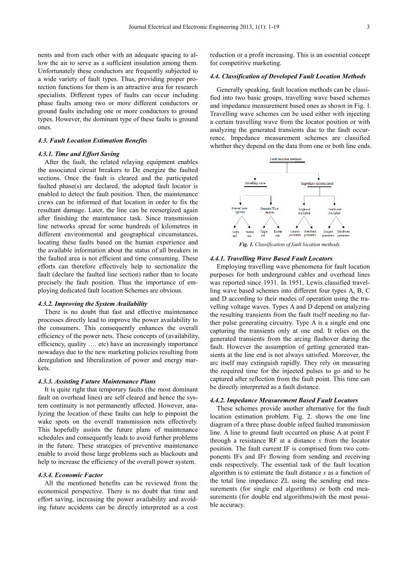
4.4. Classification of Developed Fault Location Methods
Generally speaking, fault location methods can be classi-
fied into two basic groups, travelling wave based schemes
and impedance measurement based ones as shown in Fig. 1.
Travelling wave schemes can be used either with injecting
a certain travelling wave from the locator position or with
analyzing the generated transients due to the fault occur-
rence. Impedance measurement schemes are classified
whether they depend on the data from one or both line ends.
Fig. 1. Classification of fault location methods.
4.4.1. Travelling Wave Based Fault Locators
Employing travelling wave phenomena for fault location
purposes for both underground cables and overhead lines
was reported since 1931. In 1951, Lewis classified travel-
ling wave based schemes into different four types A, B, C
and D according to their modes of operation using the tra-
velling voltage waves. Types A and D depend on analyzing
the resulting transients from the fault itself needing no fur-
ther pulse generating circuitry. Type A is a single end one
capturing the transients only at one end. It relies on the
generated transients from the arcing flashover during the
fault. However the assumption of getting generated tran-
sients at the line end is not always satisfied. Moreover, the
arc itself may extinguish rapidly. They rely on measuring
the required time for the injected pulses to go and to be
captured after reflection from the fault point. This time can
be directly interpreted as a fault distance.
4.4.2. Impedance Measurement Based Fault Locators
These schemes provide another alternative for the fault
location estimation problem. Fig. 2. shows the one line
diagram of a three phase double infeed faulted transmission
line. A line to ground fault occurred on phase A at point F
through a resistance RF at a distance x from the locator
position. The fault current IF is comprised from two com-
ponents IFs and IFr flowing from sending and receiving
ends respectively. The essential task of the fault location
algorithm is to estimate the fault distance x as a function of
the total line impedance ZL using the sending end mea-
surements (for single end algorithms) or both end mea-
surements (for double end algorithms)with the most possi-
ble accuracy.

4 Mohammad Abdul Baseer: Travelling waves for finding the fault location in transmission lines
Fig. 2. One line diagram of a faulted transmission line.
4.4.3. Non Conventional Fault Locators
Instead of the normal mathematical derivation, non con-
ventional fault location algorithms were introduced de-
pending on other processing platforms such as Wavelet
Transform (WT), ANN or GA. These methods have their
own problems that result from the line modelling accuracy,
data availability and the method essences.
4.5. Requirements for Fault Location Process
Fig. 3 presents a general explanation of the essential re-
quirements for fault locators. Generally speaking, fault
locator works in off line mode after performing the relay-
ing action. Once the fault is detected and the faulty phase(s)
are successfully classified, the fault locator is enabled to
find out the estimated fault distance. The recorded data by
the Digital Fault Recorder (DFR) is passed through the
locator input manipulator to the fault locator.
Fig. 3. General requirements for fault location schemes.
5. Travelling Wave Theory
Studies of transient disturbances on transmission sys-
tems have shown that changes are followed by travelling
waves, which at first approximation can be treated as step
front waves. As this research is focused on travelling wave
based fault location, it was decided to employ an introduc-
tory chapter to the basic theory of travelling waves.
5.1. Introduction
The transmission line conductors have resistances and
inductances distributed uniformly along the length of the
line. Travelling wave fault location methods are usually
more suitable for application to long lines.
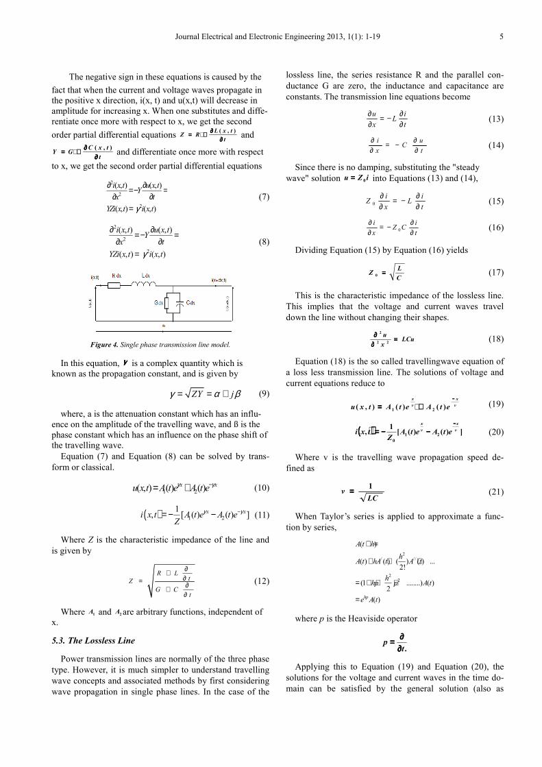
5.2. The Transmission Line Equation
A transmission line is a system of conductors connecting
one point to another and along which electromagnetic
energy can be sent. Power transmission lines are a typical
example of transmission lines. The transmission line equa-
tions that govern general two conductor uniform transmis-
sion lines, including two and three wire lines, and coaxial
cables, are called the telegraph equations. The general
transmission line equations are named the telegraph equa-
tions because they were formulated for the first time by
Oliver Heaviside (1850 1925) when he was employed by a
telegraph company and used to investigate disturbances on
telephone wires. When one considers a line segment dx
with parameters resistance ( R ), conductance ( G ), induc-
tance ( L ), and capacitance ( C ), all per unit length, (see
Figure 2.1 the line constants for segment dx are R dx, G dx,
L dx, and C dx . The electric flux ψ and the magnetic flux
φ created by the electromagnetic wave, which causes the
instantaneous voltage u(x,t) and current i(x,t), are
d ψ ( t ) = u ( x, t ) C d x (1)
And
d φ (t) = i (x, t) L d x (2)
Calculating the voltage drop in the positive direction of x
of the distance dx obtains
( , ) ( , )
( , )( , )
( ) ( , )
u x t u x dx t
u x tdu x t dx
x
R L i x t dxt
− + =∂− = − =
∂∂+∂
(3)
If dx is cancelled from both sides of (3), the voltage equ-
ation becomes
( , )
( , )( , )
u x t
x
i x tL Ri x t
t
∂ =∂∂− −
∂
(4)
Similarly, for the current owing through G and the cur-
rent charging C, Kirchhoff’s current law can be applied as
( , ) ( , )
( , )( , )
( ) ( , )
i x t i x dx t
i x tdi x t
x
G C u x t dxt
− + =∂− = − =
∂∂+∂
(5)
If dx is cancelled from both sides of (5), the current equ-
ation becomes
( , )
( , )( , )
i x t
x
u x tC Gu x t
t
∂ =∂∂− −
∂
(6)
Journal Electrical and Electronic Engineering 2013, 1(1): 1-19 5
The negative sign in these equations is caused by the
fact that when the current and voltage waves propagate in
the positive x direction, i(x, t) and u(x,t) will decrease in
amplitude for increasing x. When one substitutes and diffe-
rentiate once more with respect to x, we get the second
order partial differential equations t
txLRZ
∂∂∂∂∂∂∂∂++++====
),( and
t
txCGY
∂∂∂∂∂∂∂∂++++====
),( and differentiate once more with respect
to x, we get the second order partial differential equations
2
2
2
( , ) ( , )
( , ) ( , )
i x t u x tY
tx
YZi x t i x tγ
∂ ∂=− =∂∂
= (7)
2
2
2
( , ) ( , )
( , ) ( , )
i x t u x tY
tx
YZi x t i x tγ
∂ ∂=− =∂∂
= (8)
Figure 4. Single phase transmission line model.
In this equation, γγγγ is a complex quantity which is
known as the propagation constant, and is given by
ZY jγ α β= = + (9)
where, a is the attenuation constant which has an influ-
ence on the amplitude of the travelling wave, and ß is the
phase constant which has an influence on the phase shift of
the travelling wave.
Equation (7) and Equation (8) can be solved by trans-
form or classical.
1 2( , ) ( ) ( )x xu x t A t e A t eγ γ−= + (10)
( ) 1 2
1, [ ( ) ( ) ]x xi x t A t e A t e
Z
γ γ−= − − (11)
Where Z is the characteristic impedance of the line and
is given by
R LtZ
G Ct
∂+∂= ∂+∂
(12)
Where 1A and 2A are arbitrary functions, independent of
x.
5.3. The Lossless Line
Power transmission lines are normally of the three phase
type. However, it is much simpler to understand travelling
wave concepts and associated methods by first considering
wave propagation in single phase lines. In the case of the
lossless line, the series resistance R and the parallel con-
ductance G are zero, the inductance and capacitance are
constants. The transmission line equations become
u iL
x t
∂ ∂= −∂ ∂
(13)
i uC
x t
∂ ∂= −∂ ∂
(14)
Since there is no damping, substituting the "steady
wave" solution iZu 0==== into Equations (13) and (14),
0
i iZ L
x t
∂ ∂= −∂ ∂
(15)
0
i iZ C
x t
∂ ∂= −∂ ∂
(16)
Dividing Equation (15) by Equation (16) yields
C
LZ ====0 (17)
This is the characteristic impedance of the lossless line.
This implies that the voltage and current waves travel
down the line without changing their shapes.
LCux
u ====∂∂∂∂∂∂∂∂
22
2
(18)
Equation (18) is the so called travellingwave equation of
a loss less transmission line. The solutions of voltage and
current equations reduce to
v
x
v
x
etAetAtxu
−−−−
++++==== )()(),( 21 (19)
(((( )))) ])()([1
, 21
0
v
x
v
x
etAetAZ
txi
−−−−
−−−−−−−−==== (20)
Where v is the travelling wave propagation speed de-
fined as
LCv
1==== (21)
When Taylor’s series is applied to approximate a func-
tion by series,
2/ //
22
( )
( ) ( ) ( ) ( ) ...2!
(1 ........) ( )2
( )hp
A t h
hA t hA t A t
hhp p A t
e A t
+ =
+ + +
= + + +
=
where p is the Heaviside operator
.tp
∂∂∂∂∂∂∂∂====
Applying this to Equation (19) and Equation (20), the
solutions for the voltage and current waves in the time do-
main can be satisfied by the general solution (also as
6 Mohammad Abdul Baseer: Travelling waves for finding the fault location in transmission lines
showed by D’Alembert )
)()(),( 21v
xtA
v
xtAtxu −−−−++++++++==== (23)
)]()([1
),( 21
0 v
xtA
v
xtA
Ztxi −−−−−−−−++++−−−−==== (24)
In this expression, )(1v
xtA ++++ is a function describing a
wave propagating in the negative x direction, usually
called the backward wave, and v
xtA −−−−(2 ) is a function de-
scribing a wave propagating in the positive x direction,
called the forward wave.
5.4. Propagation Speed
From the voltage drop equation,
t
txiLdxtdxutxu
∂∂∂∂∂∂∂∂====++++−−−−
),()(),(),( (25)
Since iZu 0==== then
t
txidx
Z
Ltdxxitxi
∂∂∂∂∂∂∂∂====++++−−−−
),()(),(),(
0
(26)
Making t
txi
∂∂∂∂∂∂∂∂ ),(
finite we get
t
tdxxitxidx
Z
Ltdxxitxi
∂∂∂∂++++−−−−====++++−−−−
),(),()(),(),(
0
(27)
If the wave propagates intact
LCv
L
Z
dt
dxv
10 ============ (28)
This is the travelling wave propagation speed.
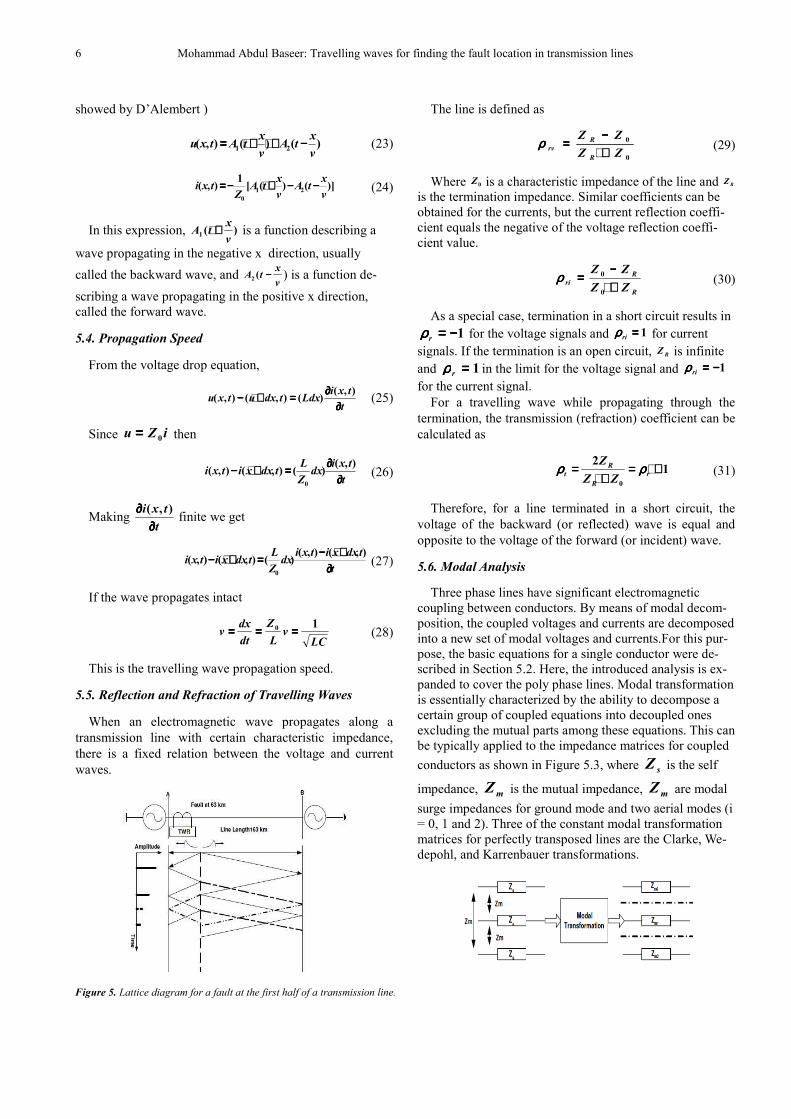
5.5. Reflection and Refraction of Travelling Waves
When an electromagnetic wave propagates along a
transmission line with certain characteristic impedance,
there is a fixed relation between the voltage and current
waves.
Figure 5. Lattice diagram for a fault at the first half of a transmission line.
The line is defined as
0
0
ZZ
ZZ
R
R
rv ++++−−−−
====ρρρρ (29)
Where 0Z is a characteristic impedance of the line and RZ
is the termination impedance. Similar coefficients can be
obtained for the currents, but the current reflection coeffi-
cient equals the negative of the voltage reflection coeffi-
cient value.
R
R
riZZ
ZZ
++++−−−−====
0
0ρρρρ (30)
As a special case, termination in a short circuit results in
1−−−−====rρρρρ for the voltage signals and 1====riρρρρ for current
signals. If the termination is an open circuit, RZ is infinite
and 1====rρρρρ in the limit for the voltage signal and 1−−−−====riρρρρ
for the current signal.
For a travelling wave while propagating through the
termination, the transmission (refraction) coefficient can be
calculated as
12
0
++++====++++
==== r
R
R
tZZ
Z ρρρρρρρρ (31)
Therefore, for a line terminated in a short circuit, the
voltage of the backward (or reflected) wave is equal and
opposite to the voltage of the forward (or incident) wave.
5.6. Modal Analysis
Three phase lines have significant electromagnetic
coupling between conductors. By means of modal decom-
position, the coupled voltages and currents are decomposed
into a new set of modal voltages and currents.For this pur-
pose, the basic equations for a single conductor were de-
scribed in Section 5.2. Here, the introduced analysis is ex-
panded to cover the poly phase lines. Modal transformation
is essentially characterized by the ability to decompose a
certain group of coupled equations into decoupled ones
excluding the mutual parts among these equations. This can
be typically applied to the impedance matrices for coupled
conductors as shown in Figure 5.3, where sZ is the self
impedance, mZ is the mutual impedance, mZ are modal
surge impedances for ground mode and two aerial modes (i
= 0, 1 and 2). Three of the constant modal transformation
matrices for perfectly transposed lines are the Clarke, We-
depohl, and Karrenbauer transformations.
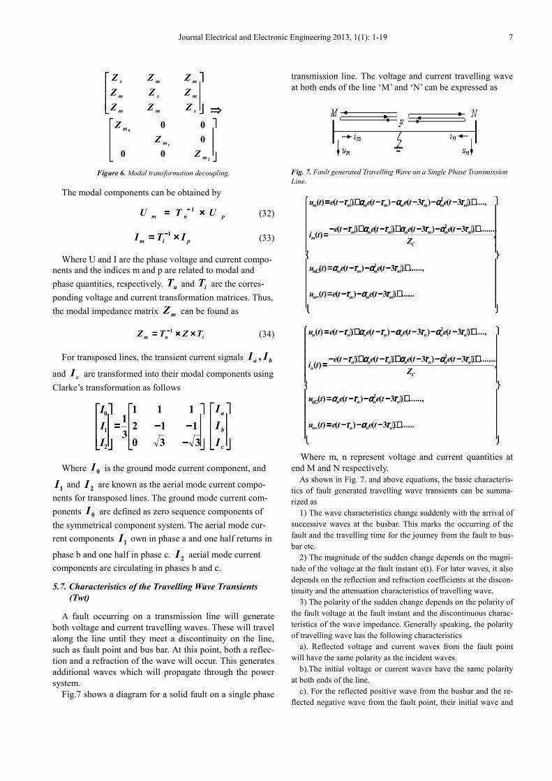
Journal Electrical and Electronic Engineering 2013, 1(1): 1-19 7
smm
msm
mms
ZZZ
ZZZ
ZZZ
⇒⇒⇒⇒
2
1
0
00
0
00
m
m
m
Z
Z
Z
Figure 6. Modal transformation decoupling.
The modal components can be obtained by
pum UTU ××××==== −−−− 1 (32)
pim ITI ××××==== −−−−1 (33)
Where U and I are the phase voltage and current compo-
nents and the indices m and p are related to modal and
phase quantities, respectively. uT and iT are the corres-
ponding voltage and current transformation matrices. Thus,
the modal impedance matrix mZ can be found as
ium TZTZ ××××××××==== −−−−1 (34)
For transposed lines, the transient current signals ba II ,
and cI are transformed into their modal components using
Clarke’s transformation as follows
−−−−−−−−−−−−====
330
112
111
3
1
2
1
0
I
I
I
c
b
a
I
I
I
Where 0I is the ground mode current component, and
1I and 2I are known as the aerial mode current compo-
nents for transposed lines. The ground mode current com-
ponents 0I are defined as zero sequence components of
the symmetrical component system. The aerial mode cur-
rent components 1I own in phase a and one half returns in
phase b and one half in phase c. 2I aerial mode current
components are circulating in phases b and c.
5.7. Characteristics of the Travelling Wave Transients
(Twt)
A fault occurring on a transmission line will generate
both voltage and current travelling waves. These will travel
along the line until they meet a discontinuity on the line,
such as fault point and bus bar. At this point, both a reflec-
tion and a refraction of the wave will occur. This generates
additional waves which will propagate through the power
system.
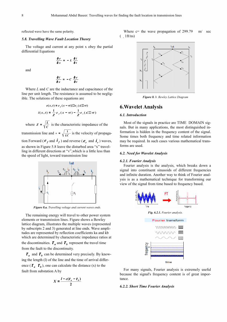
Fig.7 shows a diagram for a solid fault on a single phase
transmission line. The voltage and current travelling wave
at both ends of the line ‘M’ and ‘N’ can be expressed as
Fig. 7. Fault generated Travelling Wave on a Single Phase Transmission
Line.
++++−−−−−−−−−−−−====
++++−−−−−−−−−−−−====
++++−−−−−−−−−−−−++++−−−−++++−−−−−−−−====
++++−−−−−−−−−−−−−−−−−−−−++++−−−−====
−−−−
++++
......)3()()(
......,)3()()(
,........)3()3()()(
)(
....,)3()3()()()(
2
2
2
mmmm
mmmmm
C
mmmmmmm
m
mmmmmmmm
tetetu
tetetu
Z
teteteteti
tetetetetu
ττττααααττττ
τττταααατττταααα
ττττααααττττααααττττααααττττ
ττττααααττττααααττττααααττττ
++++−−−−−−−−−−−−====
++++−−−−−−−−−−−−====
++++−−−−−−−−−−−−++++−−−−++++−−−−−−−−====
++++−−−−−−−−−−−−−−−−−−−−++++−−−−====
−−−−
++++
......)3()()(
......,)3()()(
,........)3()3()()(
)(
....,)3()3()()()(
2
2
2
nnnn
nnnnn
C
nnnnnnn
n
nnnnnnnn
tetetu
tetetu
Z
teteteteti
tetetetetu
ττττααααττττ
τττταααατττταααα
ττττααααττττααααττττααααττττ
ττττααααττττααααττττααααττττ
Where m, n represent voltage and current quantities at
end M and N respectively.
As shown in Fig. 7. and above equations, the basic characteris-
tics of fault generated travelling wave transients can be summa-
rized as
1) The wave characteristics change suddenly with the arrival of
successive waves at the busbar. This marks the occurring of the
fault and the travelling time for the journey from the fault to bus-
bar etc.
2) The magnitude of the sudden change depends on the magni-
tude of the voltage at the fault instant e(t). For later waves, it also
depends on the reflection and refraction coefficients at the discon-
tinuity and the attenuation characteristics of travelling wave.
3) The polarity of the sudden change depends on the polarity of
the fault voltage at the fault instant and the discontinuous charac-
teristics of the wave impedance. Generally speaking, the polarity
of travelling wave has the following characteristics
a). Reflected voltage and current waves from the fault point
will have the same polarity as the incident waves.
b).The initial voltage or current waves have the same polarity
at both ends of the line.
c). For the reflected positive wave from the busbar and the re-
flected negative wave from the fault point, their initial wave and
8 Mohammad Abdul Baseer: Travelling waves for finding the fault location in transmission lines
reflected wave have the same polarity.
5.8. Travelling Wave Fault Location Theory
The voltage and current at any point x obey the partial
differential Equations
t
iL
x
e
∂∂∂∂∂∂∂∂−−−−====
∂∂∂∂∂∂∂∂
and
t
eC
x
i
∂∂∂∂∂∂∂∂−−−−====
∂∂∂∂∂∂∂∂
Where L and C are the inductance and capacitance of the
line per unit length. The resistance is assumed to be neglig-
ible. The solutions of these equations are
)()(),( vtxevtxetxe rf ++++++++−−−−====
)(1
)(1
),( vtxeZ
vtxeZ
txi rf ++++−−−−−−−−====
where C
LZ ==== is the characteristic impedance of the
transmission line and LC
v1==== is the velocity of propaga-
tion Forward ( fe and fi ) and reverse (re and
ri ) waves,
as shown in Figure 5.8 leave the disturbed area “x” travel-
ling in different directions at “v”,which is a little less than
the speed of light, toward transmission line
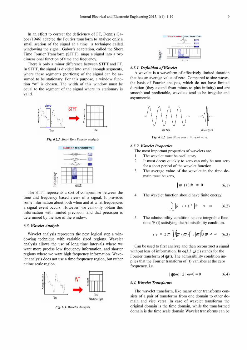
Figure 8.a. Travelling voltage and current waves ends.
The remaining energy will travel to other power system
elements or transmission lines. Figure shows a Bewley
lattice diagram, illustrates the multiple waves (represented
by subscripts 2 and 3) generated at line ends. Wave ampli-
tudes are represented by reflection coefficients ka and kb
which are determined by characteristic impedance ratios at
the discontinuities. aττττ and bττττ represent the travel time
from the fault to the discontinuity.
aττττ and bττττ can be determined very precisely. By know-
ing the length (l) of the line and the time of arrival differ-
ence ( aττττ bττττ ), one can calculate the distance (x) to the
fault from substation A by
2
)( baclX
ττττττττ −−−−−−−−====
Where c= the wave propagation of 299.79 m/ sec
( 1ft/ns)
Figure 8. b. Bewley Lattice Diagram
6.Wavelet Analysis
6.1. Introduction
Most of the signals in practice are TIME DOMAIN sig-
nals. But in many applications, the most distinguished in-
formation is hidden in the frequency content of the signal.
Some times both frequency and time related information
may be required. In such cases various mathematical trans-
forms are used.
6.2. Need for Wavelet Analysis
6.2.1. Fourier Analysis
Fourier analysis is the analysis, which breaks down a
signal into constituent sinusoids of different frequencies
and infinite duration. Another way to think of Fourier anal-
ysis is as a mathematical technique for transforming our
view of the signal from time based to frequency based.
Fig. 6.2.1. Fourier analysis.
For many signals, Fourier analysis is extremely useful
because the signal's frequency content is of great impor-
tance.
6.2.2. Short Time Fourier Analysis
Journal Electrical and Electronic Engineering 2013, 1(1): 1-19 9
In an effort to correct the deficiency of FT, Dennis Ga-
bor (1946) adapted the Fourier transform to analyze only a
small section of the signal at a time a technique called
windowing the signal. Gabor’s adaptation, called the Short
Time Fourier Transform (STFT), maps a signal into a two
dimensional function of time and frequency.
There is only a minor difference between STFT and FT.
In STFT, the signal is divided into small enough segments,
where these segments (portions) of the signal can be as-
sumed to be stationary. For this purpose, a window func-
tion “w” is chosen. The width of this window must be
equal to the segment of the signal where its stationary is
valid.
Fig. 6.2.2. Short Time Fourier analysis.
The STFT represents a sort of compromise between the
time and frequency based views of a signal. It provides
some information about both when and at what frequencies
a signal event occurs. However, we can only obtain this
information with limited precision, and that precision is
determined by the size of the window.
6.3. Wavelet Analysis
Wavelet analysis represents the next logical step a win-
dowing technique with variable sized regions. Wavelet
analysis allows the use of long time intervals where we
want more precise low frequency information, and shorter
regions where we want high frequency information. Wave-
let analysis does not use a time frequency region, but rather
a time scale region.
Fig. 6.3. Wavelet Analysis.
6.3.1. Definition of Wavelet
A wavelet is a waveform of effectively limited duration
that has an average value of zero. Compared to sine waves,
the basis of Fourier analysis, which do not have limited
duration (they extend from minus to plus infinity) and are
smooth and predictable, wavelets tend to be irregular and
asymmetric.
Fig. 6.3.1. Sine Wave and a Wavelet wave.
6.3.2. Wavelet Properties
The most important properties of wavelets are
1. The wavelet must be oscillatory.
2. It must decay quickly to zero can only be non zero
for a short period of the wavelet function
3. The average value of the wavelet in the time do-
main must be zero,
0)( =∫ dttψ (6.1)
4. The wavelet function should have finite energy.
∞<∫∞
∞−
dtt 2)(ψ (6.2)
5. The admissibility condition square integrable func-
tions Ψ (t) satisfying the Admissibility condition.
( ) ∞<= ∫∞
∞−
ωωωψπψ dc /)(22
(6.3)
Can be used to first analyze and then reconstruct a signal
without loss of information. In eq3.3 ψ(ω) stands for the
Fourier transform of ψ(t). The admissibility condition im-
plies that the Fourier transform of (t) vanishes at the zero
frequency, i.e.
| ψ(ω) | 2 | ω=0 = 0 (6.4)
6.4. Wavelet Transforms
The wavelet transform, like many other transforms con-
sists of a pair of transforms from one domain to other do-
main and vice versa. In case of wavelet transforms the
original domain is the time domain, while the transformed
domain is the time scale domain Wavelet transforms can be

10 Mohammad Abdul Baseer: Travelling waves for finding the fault location in transmission lines
accomplished in 2 different ways.
6.5. The Continuous Wavelet Transform
Mathematically, the process of Fourier analysis is
represented by the Fourier transform
(6.5)
Which is the sum over all time of the signal f (t) multip-
lied by a complex exponential. Next this complex exponen-
tial can be broken down into real and imaginary sinusoidal
components.
The results of the transform are the Fourier coefficients,
which when multiplied by a sinusoid of frequency ω, yield
the constituent sinusoidal components of the original signal.
Graphically, the process looks like shown in Figure below
Fig. 6.5(a) Breaking the signal into sine waves of different amplitudes
using FT.
Similarly, the continuous wavelet transform (CWT) is
defined as the sum over all time of the signal multiplied by
scaled, shifted versions of the wavelet function. The results
of the CWT are many wavelet coefficients C, which are a
function of scale and position.
Multiplying each coefficient by the appropriately scaled
and shifted wavelet yields the constituent wavelets of the
original signal
Fig. 6.5(b) Breaking the signal into wavelets of different amplitudes using
WT.
Mathematically CWT is given by
Where
,( , ) ( ) ( )a bCWT a b x t t dtψ∞
−∞
= ∗∫
, ( ) (( ) / )a b t t b a aψ ψ= −
Ψ (t) is the base function or the mother wavelet, the aste-
risk denotes a complex conjugate, and a,b Є R, a ≠ 0, are
the dilation and translation parameters respectively
6.5.1. Scaling
Wavelet analysis produces a time scale view of a signal.
Scaling a wavelet simply means stretching (or compressing)
it. The scale factor, often denoted by the letter a. for exam-
ple, the effect of the scale factor with wavelets is, the
smaller the scale factor, the more” compressed” the wave-
let.
Fig. 6.5.1. Wavelets of different scales.
6.5.2. Shifting
Shifting a wavelet simply means delaying (or hastening)
its onset. Mathematically, delaying a function Ψ (t) by k is
represented by Ψ (t k) and is shown in Fig6.5.2.
Fig. 6.5.2. delaying a wavelet function by k.
6.5.3. Scale and Frequency
The higher scales correspond to the most “stretched”
wavelets. The more stretched the wavelet, the longer the
portion of the signal with which it is being compared, and
thus the coarser the signal features being measured by the
wavelet coefficients.
Thus, there is a correspondence between wavelet scales
and frequency as revealed by wavelet analysis
Fig. 6.5.3. Relation between scale and frequency of the signal.
Journal Electrical and Electronic Engineering 2013, 1(1): 1-19 11
6.6. The Discrete Wavelet Transform (DWT)
6.6.1. Need for Discrete Wavelet Transform
Although the discretized continuous wavelets transform
enables the computation of the continuous wavelet trans-
forms by computers, it is not a true discrete transform.
The DWT is considerably easier to implement when
compared to the CWT. the basic concepts of the DWT will
be introduced in this section along with its properties and
the algorithms used to compute it.
6.6.2. The Discrete Wavelet Transforms (DWT)
The foundations of the DWT go back to 1976 when
croiser, esteban, and galand devised a technique to decom-
pose discrete time signals. Crochiere, Weber, and Flanagan
did a similar work on coding of speech signals in the same
year. They named their analysis scheme as sub band cod-
ing. .And the discrete wavelet transform is given by
0 0 00
( , )
[ ] ( / 2m
k
D W T m n
k n a bx k m a ma
ψ
=
−∗ − ∑
(6.8)
By comparing the eq (6.8) with general equation for im-
pulse response (FIR) digital filter
∑ −=k
cknhkxny /][][)( (6.9)
It can be seen that Ψ (k) is the impulse response of Low
pass digital filter with transfer function Ψ (ω). For a0 = 2,
each dilation of Ψ (k) effectively halves the bandwidth of
Ψ (ω). Multilevel DWT filter banks implement the DWT
eqn (6.9) in the forward transform stage and the IDWT in
the reverse transform stage.
By careful selection of a0 and b0, the family of dilated
mother wavelets constitutes an orthonormal basis of L2 (R).
6.7. Filter Bank
A time scale representation of a digital signal is obtained
using digital filtering techniques. The DWT analyzes the
signal at different frequency bands with different resolu-
tions by decomposing the signal into a coarse approxima-
tion and detail information. Their sum is the DWT.
Figure 6.7. Wavelet transform filter bank.
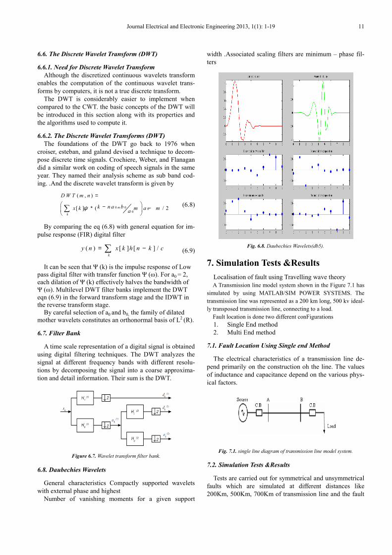
6.8. Daubechies Wavelets
General characteristics Compactly supported wavelets
with external phase and highest
Number of vanishing moments for a given support
width .Associated scaling filters are minimum – phase fil-
ters
Fig. 6.8. Daubechies Wavelets(db5).
7. Simulation Tests &Results
Localisation of fault using Travelling wave theory
A Transmission line model system shown in the Figure 7.1 has
simulated by using MATLAB/SIM POWER SYSTEMS. The
transmission line was represented as a 200 km long, 500 kv ideal-
ly transposed transmission line, connecting to a load.
Fault location is done two different conFigurations
1. Single End method
2. Multi End method
7.1. Fault Location Using Single end Method
The electrical characteristics of a transmission line de-
pend primarily on the construction oh the line. The values
of inductance and capacitance depend on the various phys-
ical factors.
Fig. 7.1. single line diagram of transmission line model system.
7.2. Simulation Tests &Results
Tests are carried out for symmetrical and unsymmetrical
faults which are simulated at different distances like
200Km, 500Km, 700Km of transmission line and the fault

12 Mohammad Abdul Baseer: Travelling waves for finding the fault location in transmission lines
localisation estimated using Travelling Wave Theory.
Difference in Time = 12 tt −
LCV
1=
is the velocity of propagation.
Distance = Velocity * Time
%Error between the actual and obtained distances is cal-
culated as
The various faults considered are
1. Line to ground (L G) fault,
2. Double line (L L) fault,
3. Double line to ground (L L G) fault,
4. 3 Φ (or L L L) fault, and
5. 3 Φ to ground (or L L L G) fault.
Tables 1,2 & 3 shows the calculated fault distances by
using TWT
Table 1. Location of Faults using single end method for a 200Km Trans-
mission line.
Table 2. Location of Faults using single end method for a for a 500Km
Transmission line.
Table 3. Location of Faults using single end method for a for a 700Km
Transmission line.
7.2.1. Case I. Specifications of a 200Km Transmission
Line
Source Voltage 500kV, 50Hz
Transmission Line Length 200Km, distributed parameter
transmission line model
R1 = 0.01273 Ω/km; R0 = 0.3864 Ω/km;
L1 = 0.9337e 3 H/km; L0 = 4.1264e 3 H/km;
C1 = 12.74e 9 F/km C0 = 7.751e 9 F/km
Fault is created at 0.0006 and cleared at 0.0009, simula-
tion time 0.0015
Fig. 7.2.1(b) Voltage wave form, for L G fault at 100km.
The voltage waveform in Figrepresents an L G fault
created at distance of 100km on a transmission line of
200km long, the fault creation time is 0.0006 sec and the
shift in voltage wave form appears at 0.000934sec this is
due to the travelling time taken by the fault to appear at the
relay point.
7.2.2. Case II. Specifications of A 500Km Length Line
with Distributed Parameters
Source Voltage 500kV, 50Hz
Transmission Line Length 500Km, distributed parameter
transmission line model
Journal Electrical and Electronic Engineering 2013, 1(1): 1-19 13
R1 = 0.01273 Ω/km; R0 = 0.3864 Ω/km;
L1 = 0.9337e 3 H/km; L0 = 4.1264e 3 H/km;
C1 = 12.74e 9 F/km C0 = 7.751e 9 F/km
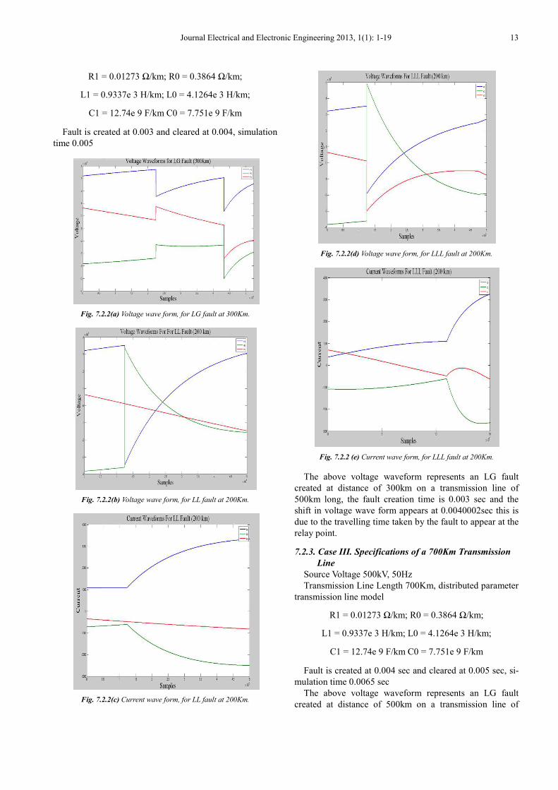
Fault is created at 0.003 and cleared at 0.004, simulation
time 0.005
Fig. 7.2.2(a) Voltage wave form, for LG fault at 300Km.
Fig. 7.2.2(b) Voltage wave form, for LL fault at 200Km.
Fig. 7.2.2(c) Current wave form, for LL fault at 200Km.
Fig. 7.2.2(d) Voltage wave form, for LLL fault at 200Km.
Fig. 7.2.2 (e) Current wave form, for LLL fault at 200Km.
The above voltage waveform represents an LG fault
created at distance of 300km on a transmission line of
500km long, the fault creation time is 0.003 sec and the
shift in voltage wave form appears at 0.0040002sec this is
due to the travelling time taken by the fault to appear at the
relay point.
7.2.3. Case III. Specifications of a 700Km Transmission
Line
Source Voltage 500kV, 50Hz
Transmission Line Length 700Km, distributed parameter
transmission line model
R1 = 0.01273 Ω/km; R0 = 0.3864 Ω/km;
L1 = 0.9337e 3 H/km; L0 = 4.1264e 3 H/km;
C1 = 12.74e 9 F/km C0 = 7.751e 9 F/km
Fault is created at 0.004 sec and cleared at 0.005 sec, si-
mulation time 0.0065 sec
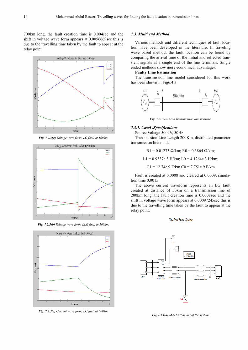
The above voltage waveform represents an LG fault
created at distance of 500km on a transmission line of
14 Mohammad Abdul Baseer: Travelling waves for finding the fault location in transmission lines
700km long, the fault creation time is 0.004sec and the
shift in voltage wave form appears at 0.0056669sec this is
due to the travelling time taken by the fault to appear at the
relay point.
Fig. 7.2.3(a) Voltage wave form, LG fault at 500km.
Fig. 7.2.3(b) Voltage wave form, LLG fault at 500km.
Fig. 7.2.3(c) Current wave form, LG fault at 500km.
7.3. Multi end Method
Various methods and different techniques of fault loca-
tion have been developed in the literature. In traveling
wave based method, the fault location can be found by
comparing the arrival time of the initial and reflected tran-
sient signals at a single end of the line terminals. Single
ended methods show more economical advantages.
Faulty Line Estimation
The transmission line model considered for this work
has been shown in Fig6.4.3
Fig. 7.3. Two Area Transmission line network.
7.3.1. CaseI .Specifications
Source Voltage 500kV, 50Hz
Transmission Line Length 200Km, distributed parameter
transmission line model
R1 = 0.01273 Ω/km; R0 = 0.3864 Ω/km;
L1 = 0.9337e 3 H/km; L0 = 4.1264e 3 H/km;
C1 = 12.74e 9 F/km C0 = 7.751e 9 F/km
Fault is created at 0.0008 and cleared at 0.0009, simula-
tion time 0.0015
The above current waveform represents an LG fault
created at distance of 50km on a transmission line of
200km long, the fault creation time is 0.0008sec and the
shift in voltage wave form appears at 0.00097245sec this is
due to the travelling time taken by the fault to appear at the
relay point.
Fig.7.3.1(a) MATLAB model of the system.
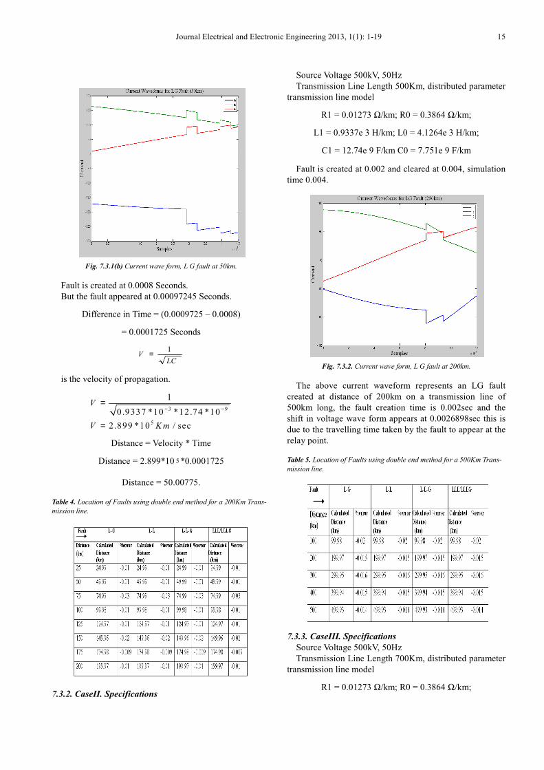
Journal Electrical and Electronic Engineering 2013, 1(1): 1-19 15
Fig. 7.3.1(b) Current wave form, L G fault at 50km.
Fault is created at 0.0008 Seconds.
But the fault appeared at 0.00097245 Seconds.
Difference in Time = (0.0009725 – 0.0008)
= 0.0001725 Seconds
LCV
1=
is the velocity of propagation.
3 9
5
1
0.9337 *10 *12.74 *10
2.899 *10 / sec
V
V K m
− −=
=
Distance = Velocity * Time
Distance = 2.899*10 5 *0.0001725
Distance = 50.00775.
Table 4. Location of Faults using double end method for a 200Km Trans-
mission line.
7.3.2. CaseII. Specifications
Source Voltage 500kV, 50Hz
Transmission Line Length 500Km, distributed parameter
transmission line model
R1 = 0.01273 Ω/km; R0 = 0.3864 Ω/km;
L1 = 0.9337e 3 H/km; L0 = 4.1264e 3 H/km;
C1 = 12.74e 9 F/km C0 = 7.751e 9 F/km
Fault is created at 0.002 and cleared at 0.004, simulation
time 0.004.
Fig. 7.3.2. Current wave form, L G fault at 200km.
The above current waveform represents an LG fault
created at distance of 200km on a transmission line of
500km long, the fault creation time is 0.002sec and the
shift in voltage wave form appears at 0.0026898sec this is
due to the travelling time taken by the fault to appear at the
relay point.
Table 5. Location of Faults using double end method for a 500Km Trans-
mission line.
7.3.3. CaseIII. Specifications
Source Voltage 500kV, 50Hz
Transmission Line Length 700Km, distributed parameter
transmission line model
R1 = 0.01273 Ω/km; R0 = 0.3864 Ω/km;
16 Mohammad Abdul Baseer: Travelling waves for finding the fault location in transmission lines
L1 = 0.9337e 3 H/km; L0 = 4.1264e 3 H/km;
C1 = 12.74e 9 F/km C0 = 7.751e 9 F/km
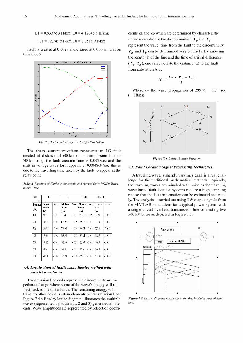
Fault is created at 0.0028 and cleared at 0.006 simulation
time 0.006
Fig. 7.3.3. Current wave form, L G fault at 600km.
The above current waveform represents an LG fault
created at distance of 600km on a transmission line of
700km long, the fault creation time is 0.0028sec and the
shift in voltage wave form appears at 0.0048694sec this is
due to the travelling time taken by the fault to appear at the
relay point.
Table 6. Location of Faults using double end method for a 700Km Trans-
mission line.
7.4. Localisation of faults using Bewley method with
wavelet transforms
Transmission line ends represent a discontinuity or im-
pedance change where some of the wave’s energy will re-
flect back to the disturbance. The remaining energy will
travel to other power system elements or transmission lines.
Figure 7.4 a Bewley lattice diagram, illustrates the multiple
waves (represented by subscripts 2 and 3) generated at line
ends. Wave amplitudes are represented by reflection coeffi-
cients ka and kb which are determined by characteristic
impedance ratios at the discontinuities. aττττ and bττττ
represent the travel time from the fault to the discontinuity.
aττττ and bττττ can be determined very precisely. By knowing
the length (l) of the line and the time of arrival difference
( aττττ bττττ ), one can calculate the distance (x) to the fault
from substation A by
2
)( baclX
ττττττττ −−−−−−−−====
Where c= the wave propagation of 299.79 m/ sec
( 1ft/ns)
Figure 7.4. Bewley Lattice Diagram.
7.5. Fault Location Signal Processing Techniques
A traveling wave, a sharply varying signal, is a real chal-
lenge for the traditional mathematical methods. Typically,
the traveling waves are mingled with noise as the traveling
wave based fault location systems require a high sampling
rate so that the fault information can be estimated accurate-
ly. The analysis is carried out using TW output signals from
the MATLAB simulations for a typical power system with
a single circuit overhead transmission line connecting two
500 kV buses as depicted in Figure 7.5.
Figure 7.5. Lattice diagram for a fault at the first half of a transmission
line.

Journal Electrical and Electronic Engineering 2013, 1(1): 1-19 17
Frequency Domain Approach
Fourier transform based fault location algorithms have
been proposed since a long time. Most of the proposed
algorithms use voltages and currents between fault initia-
tion and fault clearing. To find out the frequency contents
of the fault signal, several transformations can be applied,
namely, Fourier, STFT, and Wavelet etc.
Fourier Transform
Fourier transform (FT) is the most popular transforma-
tion that can be applied to traveling wave signals to obtain
their frequency components appearing in the fault signal.
Usually, the information that cannot be readily seen in the
time domain can be seen in the frequency domain. The FT
and its inverse give a one to one relationship between the
time domain )t(x and the frequency domain )(x ω .Given a
signal )t(I , the FT )(FT ω is defined by the following equa-
tion
dte).t(IFT tj
∫=∞
∞−
ω−
Time Frequency Domain Approach
The traveling wave based fault locators utilize high fre-
quency signals, which are filtered from the measured signal.
Discrete Fourier Transform (DFT) based spectral analysis
is the dominant analytical tool for frequency domain analy-
sis. However, the DFT cannot provide any information of
the spectrum changes with respect to time.
Short Time Fourier Transform
To overcome the shortcoming of the DFT, short time
Fourier transform (STFT, Denis Gabor, 1946) was devel-
oped. In the STFT defined below, the signal is divided into
small segments which can be assumed to be stationary. The
signal is multiplied by a window function within the Fouri-
er integral. If the window length is infinite, it becomes the
DFT.
dte).t(w).t(I),t(STFT tj
∫ τ−=ω+∞
∞−
ω−
Where )t(I is the measured signal, ω is frequency,
)t(w τ− is a window function, τ is the translation, and t
is time.
To separate the negative property of the DFT described
above, the signal is to be divided into small enough seg-
ments, where these segments (portion) of the signal can be
assumed to be stationary.
Wavelet Transform
The wavelet multiresolution analysis is a new and po-
werful method of signal analysis and is well suited to trav-
eling wave signals. Wavelets can provide multiple resolu-
tions in both time and frequency domains. The windowing
of wavelet transform is adjusted automatically for low and
high frequencies i.e., it uses short time intervals for high
frequency components and long time intervals for low fre-
quency components.
Given a function )t(x , its Continuous Wavelet Transform
(CWT) is defined as follows
dt)a
bt()t(x
a
1)b,a(CWT
* −∫ ψ==∞+
∞−
The transformed signal is a function with two variables b
and a, the translation and the scale parameter respectively. )t(ψ is the mother wavelet, which is a band pass filter and
*ψ is the complex conjugate form. The factor a
1 is used
to ensure that each scaled wavelet function has the same
energy as the wavelet basis function. It should also satisfy
the following admissible condition
∫ =ψ∞
∞−
0dt)t(
The term translation refers to the location of the window.
As the window is shifted through the signal, time informa-
tion in the transform domain is obtained. a is the scale pa-
rameter which is inversely proportional to frequency.
Wavelet transform of sampled waveforms can be obtained
by implementing the DWT, which is given by
0 0
00
( , , )
1[ ]
m
mm
DW T k n m
k nb ax n
aaψ
=
−∑
Where )t(ψ is the mother wavelet, and the scaling and
translation parameters a and b in (3 13) are replaced by m
0a
and m
00anb respectively, n and m being integer variables. In
the standard DWT, the coefficients are sampled from the
CWT on a dyadic grid.
The wavelet coefficients (WTC) of the signal are derived
using matrix equations based on decomposition and recon-
struction of a discrete signal. Actual implementation of the
DWT involves successive pairs of high pass and low pass
filters at each scaling stage of the DWT. This can be
thought of as successive approximations of the same func-
tion, each approximation providing the incremental infor-
mation related to a particular scale (frequency range). The
first scale covers a broad frequency range at the high fre-
quency end of the spectrum and the higher scales cover the
lower end of the frequency spectrum however with pro-
gressively shorter bandwidths. Conversely, the first scale
will have the highest time resolution. Higher scales will
cover increasingly longer time intervals.
7.5.1. Case I Single End
The system is simulated at different locations along the
line. A sampling time of 9103333 −−−−××××. sec is used for all si-
mulations and propagation speeds of 289900 km/s. The
voltage waveform with multiple reflections is loaded to
wavelet toolbox
The distance is calculated as
2
dtvx ====
5 5 9289900(1.849 10 0.849 10 ) 3.333 10
2
48.31
x
km
−× − × × ×=
=

18 Mohammad Abdul Baseer: Travelling waves for finding the fault location in transmission lines
for LG fault at 50km
Fig. 7.5.1(a) Voltage Waveform for L G fault at 50 km with Wavelet Trans-
form.
Fig. 7.5.1(b) Voltage Waveform for L L fault at 100 km with Wavelet
Transform.
Fig. 7.5.1(c) Voltage Waveform for L L G fault at 200 km with Wavelet
Transform.
Fig. 7.5.1(d) Voltage Waveform for Symmetrical faults at 150 km with
Wavelet Transform.
Table 7. Location of Faults using single end method for a 200km trans-
mission line with Wavelet transforms.
8. Conclusion
In this thesis presented a fault locator that is based on the
characteristics of the travelling waves initiated from the
fault. This part of the work has addressed the problem of
fault distance estimation utilising the measurements of cur-
rents as well as voltage travelling wave signals single area
and two area transmission line systems. The travelling
wave theory was introduced and the properties of the tra-
velling waves on transmission lines were also discussed.
The objective of this thesis was to propose an automated
technique based on travelling waves for finding the fault
location in transmission lines and to test the performance
of the technique. The proposed method uses the measured
fault current signals of the fault signals. The error in fault
location estimation is a function of the sampling rate and
the speed of propagation. The techniques were tested using
data generated by executing various cases in MAT-
LAB/SIMULINK. Various types of faults were applied at
various locations on the transmission lines. It is possible to
achieve greater accuracy with multi end methods devel-

Journal Electrical and Electronic Engineering 2013, 1(1): 1-19 19
oped in this manuscript compared to the traditional fault
location methods.
References
[1] Lin Yong Wu, Zheng You He, Qing Quan Qian “A New Single Ended Fault Location Technique Using Travelling Wave Natural Frequencies” Chengdu, China, 2009.
[2] Du Lin, Pang Jun, Sima wenxia, Tang Jun, Zhou jun “Fault location for transmission line based on traveling waves us-ing correlation analysis method”2008 international confe-rence on high voltage engineering and applica-tion,chongqing,china,November 9 13,2008.
[3] Bian Haihong and Xu Qingshan “Study of Fault Location for Parallel Transmissions Lines Using One Terminal Cur-rent Traveling Waves” DRPT2008 6 9 April 2008 Nanjing China.
[4] ZOU Gui bin GAO Hou lei, “Algorithm for Ultra High Speed Travelling Wave Protection with Accurate FaultLoca-tion” 2008 IEEE.
[5] Magnus Ohrstrom, Martin Geidl, Lennart Soder, Goran Andersson “evaluation of travelling wave based protection schemes for implementation in medium voltage distribution systems” C I R E D, 18 th International Conference on Elec-tricity Distribution, Turin, 6 9 June 2005.
[6] S. Jamali and A. Ghezeljeh “fault location on transmission line using high frequency travelling waves” The Institution of Electrical Engineers, Iran,2004
[7] X Z Dong, M A Redfern, Z Bo, and F Jiang “ The Applica-tion of the Wavelet Transform of Travelling Wave Pheno-mena for Transient Based Protection” International Confe-rence on Power Systems Transients – IPST 2003 in New Orleans, USA.
[8] Michael A.street “ delivery and application of precise tim-ing for a travelling wave power line fault locator system. This paper describes BPA's fault locator system” IEEE transaction power delivery.
[9] Qin Jian Chen Xiangxun Zheng Jianchao “Travelling Wave Fault Location of Transmission Line Using Wavelet Trans-form” IEEE transaction power delivery, China.
[10] N. C. Pahalawaththa, G. B. Ancell, “maximum likelihood estimation of fault location on transmission lines using tra-velling waves” IEEE Transactions on Power Delivery. Vol. 9, No. 2, April 1994.
[11] Hathaway Telefault TWS Technical Data Sheet, “Traveling wave locator”, H.V. TEST (PTY) LTD,South Africa, Online http //www hvtest co
za/Company/PDF/Hathaway/TWSMkIIIBrochure pdf
[12] T. Takagi, J. Baba, K. Uemura, T. Sakaguchi, “Fault protec-tion based on traveling wave theory, Part 1 Theory”, IEEE PES Summer Meeting, 1977, Mexico City, Mexico, Paper No. A 77, pp. 750 3.
[13] H. Dommel, J. Mitchels, “High speed relaying using travel-ing wave transient analysis”, IEEE PES Winter Power Meeting, New York, Jan. 1978, pp. 214 219.
[14] T. Takagi, J. Baba, K. Uemura, T. Sakaguchi, “Fault protec-tion based on traveling wave theory. Part 2 Sensitivity anal-ysis and laboratory test”, In IEEE PES Winter Meeting, New York City, 1978, Paper No. A 78, pp. 220 226.
[15] P.A. Crossley and P.G. McLaren, “Distance protection based on traveling waves”, IEEE Trans. Power Apparatus Syst. PAS 102 (1983), pp. 2971 2983.
[16] Y. G. Paithankar and M. T.Sant, “A new algorithm for relay-ing and fault location based on auto correlation of travelling waves ”, Electric Power Systems Research, Vol. 8, 2, March 1985, pp. 179185.
[17] E. Shehab Eldin and P.McLaren, “Traveling wave distance protection problem areas and solutions”, IEEE Trans. Power Delivery, 3, (1988), pp. 894902.
[18] S. Rajendra, P. G. McLaren, “Traveling wave techniques applied to protection of teed circuits Principle of traveling wave techniques”, IEEE Trans PAS, 1985, 104, pp. 3544-3550.
[19] S. Rajendra, P. G. McLaren, “Traveling wave techniques applied to the protection of teed circuits Multi phase/multi circuit system”,IEEE Trans PAS 1985, 104, pp. 3551 3557.
[20] [20] D. Thomas, A. Wright, “Scheme, based on travelling waves, for the protection of major transmission lines”, IEEE Proc. C, 1988, pp. 6373.
[21] C. Aguilera, E. Orduna, G. Ratta, “Adaptive Noncommuni-cation Protection Based on Traveling Waves and Impedance Relay”, IEEE Transactions on Power Delivery, Vol. 21, 3, July 2006, pp. 11541162.
[22] C. Aguilera, E. Orduna, G. Ratta, “Directional Traveling Wave Protection Based on Slope Change Analysis”, IEEE Transactions on Power Delivery, Vol. 22, 4, Oct. 2007, pp. 20252033.
[23] Power System Relaying Committee IEEE Std C37.114 2004, “IEEE Guide for Determining Fault Location on AC Trans-mission and Distribution Lines”, 2005, E ISBN 0 7381 4654 4.
[24] B. M. Weedy, B. J. Cory, “Electric Power Systems”, 4th edition, 1998, John Wiley & Sons Ltd.