Travel Time Inversion in Seismic Tomography

S. Padina, D. Churchill, R. P. Bording

March 2, 2006

1 Introduction

The word tomography finds its origins in the two Greek words tomos, meaning section, and graphy,which translates as drawing. There are many different types of tomography used in many sciencessuch as medicine, biology, materials science and geology. The basic idea of tomography in all ofits uses is to obtain a cross-section of an object which will then be used to infer various factsregarding the particular object’s internal structure.

In processing seismic data the earth internal parameters of velocity and density play a criticalrole. Seismic imaging methods all require an accurate parameter estimation process. For imagingalgorithms which are based on depth rather than time for the output, it is essential that theinterval velocities be determined in a cellular type of model rather than the traditional layeredmodel. The approach used in tomography is a natural for cellular seismic model building. In thispaper we present a dipping layer, gridded cell, ray trace tomographic system built at MemorialUniversity for determining reflection tomograms and well based tomograms. Based on Javait runs on both Windows and Linux machines and the code is open source which allows formodifications for research purposes. The second author is the primary developer of the code.More general systems are available but we feel the benefits of a graphical user interface andthe open source code will allow for development of more sophisticated tools during the life ofthis project. Further, typically available codes are not written for parallel computation of therays and the method used here is ideal for using hundreds, if not thousands of processors forthe ray tracing and the linear algebra of the least squares problem. Both of these issues willbe important when the seismic processing parameters are from three dimensional problems. Wewill illustrate the raytracing aspects of the three dimensional tomographic problem using thelarge screen visualization system in the Earth Sciences Department at Memorial University. Asa part of the development effort we are build into the ray tracing methodology a mechanismssimulate converted waves, compute the relative amplitudes for compressional and shear wavesin models that allow for acoustic, elastic, and density parameters. The research areas includeallowing certain regions in the model to be anisotropic, highly fractured, or to be visco-acousticin nature.

In the following sections we review the notion of seismic tomography, how and why travel timesare computed, the forward and inverse modeling problem, how a cellular model is developed, howthe raytracing works, the linear algebra of the travel time equation, solving the least squaresproblem using conjugate gradients, why the matrix is sparse, and some examples of ray tracingusing the Java code and an example of the user interface.

1

1.1 Seismic Tomography

Just like radiation and magnetic fields are used in medical tomography to produce an imageof the interior of the body, the same principles can be applied to imagine the interior of ourplanet. Seeing as sectional viewing of the subsurface of the earth is the ultimate goal of seismicsurveying, it makes sense for tomography to be discussed in this context. Throughout the restof this document, when used by itself, the term tomography will be taken to refer to seismictomography and not its other applications in other fields.

Seismic tomography aids in the understanding of the planet’s internal structure. However,due to the different scopes of investigations regarding said structure, most applications of seismictomography find themselves divided between two different types:

Global In global tomography scientists apply tomographic methods to data obtained naturallyfrom earthquakes (about 2 million of them) to understand the structure of the mantle—oneof the deeper layers of earth.

Near-surface This second type of seismic tomography is concerned with the shallower sub-surface, not going further than a few kilometers. Its major application is in explorationgeophysics where the subsurface is investigated in a search for specific substances such asoil. As a major difference from global tomography, this method does not rely on naturally-occuring earthquakes, but rather artificial seismic-wave sources, such as explosive detona-tions.

It is the latter of the two types of tomography that this project is concerned with. Throughout thenext sections we will further explain the basic principles of tomography along with computationalproblems and their solutions.

1.2 Travel Time Tomography

Travel time tomography is merely a more accurate way of referring to seismic tomography, onethat puts the emphasis on the key aspect used to investigate the subsurface—travel time. Theterm refers to the time it takes a seismic wave to travel into the subsurface, reach a reflectingboundary and return to the surface. As mentioned previously, the seismic waves we are deal-ing with here are artificial and caused during experiments involving the detonation of certainexplosives or other source mechanisms.

To retrieve the travel time, receivers are placed on the surface away from the source of theexplosion at predefined distances, typically in a straight line. These receivers will record anysounds that reach them along with the time of the occurrence and by using a method calledtime picking we can obtain the exact travel times of the waves from these records. Also knownas seismic reflection times, these travel times can be used to estimate the velocities at whichthe energy waves traverse the subsurface. Knowing that seismic waves are nothing more thanacoustic sound waves—the travel velocity of which is known for a certain medium—we can usethis information to determine the substances present in the subsurface and thus gain a betterunderstanding of its structure. It should be at this point noted that for such a method to besuccessful, an elementary idea of the location of the reflecting boundaries is necessary. This issuewill be mentioned again in later sections of the document.

The general procedure used in travel time tomography to determine velocities can be sum-marized as follows:

• In a primary step we perform the field experiment and we pick the time for rays that reacheach receiver thus obtaining the seismic travel times. As a remark, it should be mentioned

2

that between the source and any receiver there is usually more than one ray. The actualnumber depends on the number of reflecting boundaries.

• After retrieving the travel times we need to gain an understanding of the distances travelledto be able make any assumptions on velocities. This is where ray tracing comes to our aid.Ray tracing is a method that applies the theories of how seismic waves travel within variousmediums, the result of which is a schematic that will allow us to approximate the distancestravelled between reflection boundaries.

• In the concluding step we take the data produced by the previous two steps and constructso-called travel time equations that we then attempt to solve for velocity. This procedureis also called travel time inversion mainly because we start with experiment data and weinfer a geophysical model that could have produced it.

In the sections to come we provide a more detailed explanation of the procedure described above.

1.3 Forward Modeling vs Inversion

In the previous section, the term travel time inversion was introduced and we provide here asection to explain the general differences between forward modeling and inversion for the readerto gain a better understanding of the opposing yet intertwining usage of the two methods inseismic tomography.

Forward modeling is a method the results of which are a prediction of the data an experimentwould produce were to be performed. For this we need to have an accurate description of thegeology of the subsurface we are studying. We then decide on what experiment we are concernedwith and we can deduce the seismic parameters for data acquisition such an experiment wouldrequire. Based on theory and physical processes we can then use the geological model and theparameters to predict the data the the experiment would produce.

On the other hand, inversion concerns itself with how to infer a model after physically runningan experiment. The known data here consists of the data acquisition parameters again and thedata the experiment produced. We then apply a series of mathematic methods to obtain adescription of the geology underlying the experiment.

While the two methods work at opposite ends (one’s known data is the other one’s aim andvice-versa) they can be combined with one working as a test for the other. This project isconcerned with the inversion problem, but once we have obtained a model, we can use it as inputfor the forward modeling process to see if it the model would predict the data we know from ourexperiment to be true.

2 Previous Work

After we had a look at the basic ideas behind seismic tomography, in this section we will detailsome of the work done in the past on this issue and that has enabled the inversion problem tobe stated in mathematical terms. This will in turn facilitate the proposal of a solution and thediscussion of its computational issues and overall feasibility.

2.1 Dividing the subsurface

In the initial stages of seismic tomography it was generally assumed that the subsurface is dividedinto different layers (Bording, 1987)—each with a constant velocity and density throughout thelayer—and that these layers were separated by flat interfaces. While this scenario makes for

3

very easy computations it is not in fact at all accurate. Later experiments have confirmed thatvelocity varies a lot within the subsurface and while there are severe differences present in someareas causing an apparent layer structure, the interfaces present between layers are not flat andone layer cannot be approximated by having constant parameters throughout. This means thatthe velocity with which a seismic wave would travel within a layer does not stay the same allthroughout.

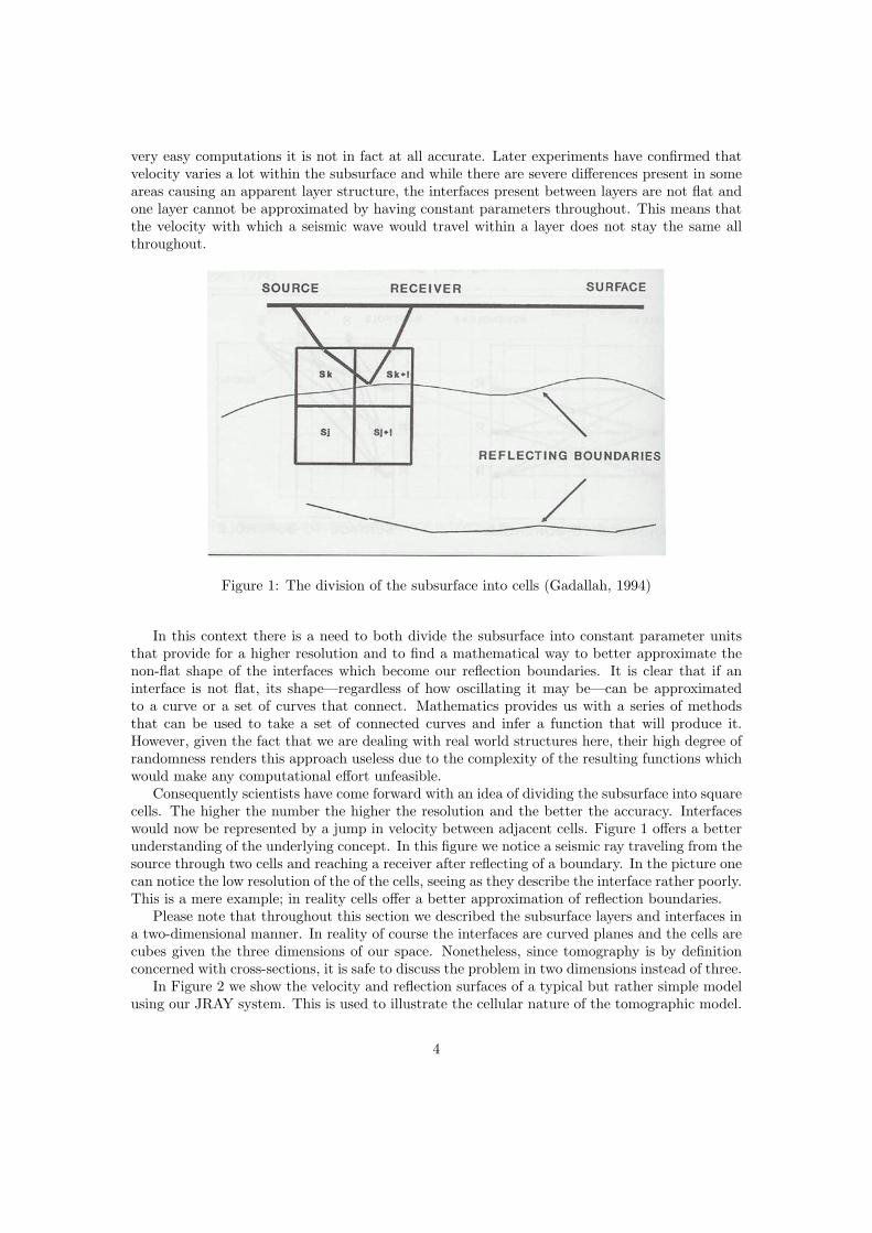
Figure 1: The division of the subsurface into cells (Gadallah, 1994)

In this context there is a need to both divide the subsurface into constant parameter unitsthat provide for a higher resolution and to find a mathematical way to better approximate thenon-flat shape of the interfaces which become our reflection boundaries. It is clear that if aninterface is not flat, its shape—regardless of how oscillating it may be—can be approximatedto a curve or a set of curves that connect. Mathematics provides us with a series of methodsthat can be used to take a set of connected curves and infer a function that will produce it.However, given the fact that we are dealing with real world structures here, their high degree ofrandomness renders this approach useless due to the complexity of the resulting functions whichwould make any computational effort unfeasible.

Consequently scientists have come forward with an idea of dividing the subsurface into squarecells. The higher the number the higher the resolution and the better the accuracy. Interfaceswould now be represented by a jump in velocity between adjacent cells. Figure 1 offers a betterunderstanding of the underlying concept. In this figure we notice a seismic ray traveling from thesource through two cells and reaching a receiver after reflecting of a boundary. In the picture onecan notice the low resolution of the of the cells, seeing as they describe the interface rather poorly.This is a mere example; in reality cells offer a better approximation of reflection boundaries.

Please note that throughout this section we described the subsurface layers and interfaces ina two-dimensional manner. In reality of course the interfaces are curved planes and the cells arecubes given the three dimensions of our space. Nonetheless, since tomography is by definitionconcerned with cross-sections, it is safe to discuss the problem in two dimensions instead of three.

In Figure 2 we show the velocity and reflection surfaces of a typical but rather simple modelusing our JRAY system. This is used to illustrate the cellular nature of the tomographic model.

4

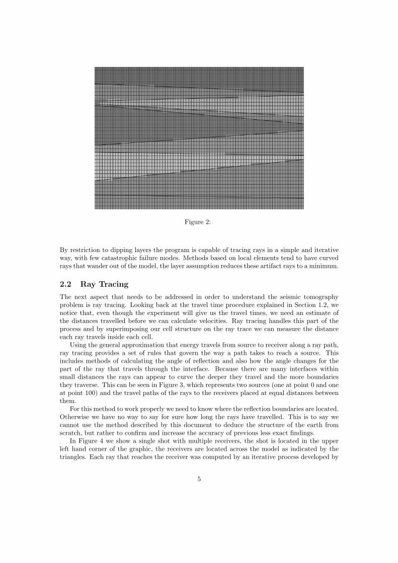
Figure 2:

By restriction to dipping layers the program is capable of tracing rays in a simple and iterativeway, with few catastrophic failure modes. Methods based on local elements tend to have curvedrays that wander out of the model, the layer assumption reduces these artifact rays to a minimum.

2.2 Ray Tracing

The next aspect that needs to be addressed in order to understand the seismic tomographyproblem is ray tracing. Looking back at the travel time procedure explained in Section 1.2, wenotice that, even though the experiment will give us the travel times, we need an estimate ofthe distances travelled before we can calculate velocities. Ray tracing handles this part of theprocess and by superimposing our cell structure on the ray trace we can measure the distanceeach ray travels inside each cell.

Using the general approximation that energy travels from source to receiver along a ray path,ray tracing provides a set of rules that govern the way a path takes to reach a source. Thisincludes methods of calculating the angle of reflection and also how the angle changes for thepart of the ray that travels through the interface. Because there are many interfaces withinsmall distances the rays can appear to curve the deeper they travel and the more boundariesthey traverse. This can be seen in Figure 3, which represents two sources (one at point 0 and oneat point 100) and the travel paths of the rays to the receivers placed at equal distances betweenthem.

For this method to work properly we need to know where the reflection boundaries are located.Otherwise we have no way to say for sure how long the rays have travelled. This is to say wecannot use the method described by this document to deduce the structure of the earth fromscratch, but rather to confirm and increase the accuracy of previous less exact findings.

In Figure 4 we show a single shot with multiple receivers, the shot is located in the upperleft hand corner of the graphic, the receivers are located across the model as indicated by thetriangles. Each ray that reaches the receiver was computed by an iterative process developed by

5

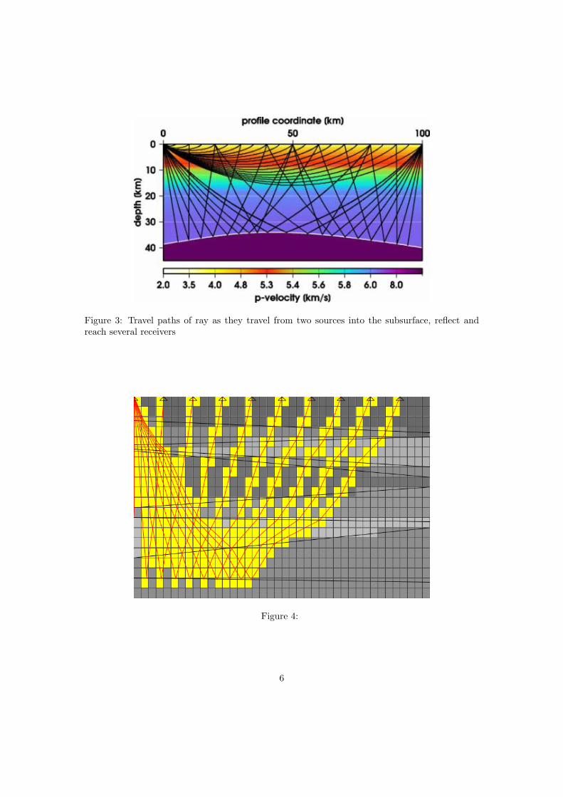
Figure 3: Travel paths of ray as they travel from two sources into the subsurface, reflect andreach several receivers

Figure 4:

6

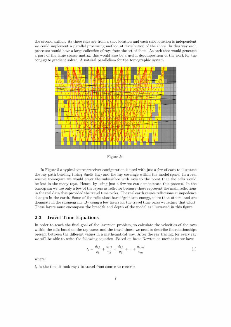
the second author. As these rays are from a shot location and each shot location is independentwe could implement a parallel processing method of distribution of the shots. In this way eachprocessor would have a large collection of rays from the set of shots. As each shot would generatea part of the large sparse matrix, this would also be a useful decomposition of the work for theconjugate gradient solver. A natural parallelism for the tomographic system.

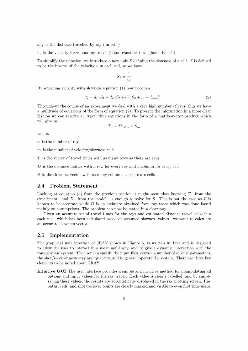
Figure 5:

In Figure 5 a typical source/receiver configuration is used with just a few of each to illustratethe ray path bending (using Snells law) and the ray coverage within the model space. In a realseismic tomogram we would cover the subsurface with rays to the point that the cells wouldbe lost in the many rays. Hence, by using just a few we can demonstrate this process. In thetomogram we use only a few of the layers as reflector because those represent the main reflectionsin the real data that provided the travel time picks. The real earth causes reflections at impedencechanges in the earth. Some of the reflections have significant energy, more than others, and aredominate in the seismogram. By using a few layers for the travel time picks we reduce that effort.These layers must encompass the breadth and depth of the model as illustrated in this figure.

2.3 Travel Time Equations

In order to reach the final goal of the inversion problem, to calculate the velocities of the rayswithin the cells based on the ray traces and the travel times, we need to describe the relationshipspresent between the different values in a mathematical way. After the ray tracing, for every raywe will be able to write the following equation. Based on basic Newtonian mechanics we have

ti =di,1

v1+

di,2

v2+

di,3

v3+ ... +

di,m

vm(1)

where:

ti is the time it took ray i to travel from source to receiver

7

di,j is the distance travelled by ray i in cell j

vj is the velocity corresponding to cell j (and constant throughout the cell)

To simplify the notation, we introduce a new unit S defining the slowness of a cell. S is definedto be the inverse of the velocity v in each cell, so we have

Sj =1vj

By replacing velocity with slowness equation (1) now becomes

ti = di,1S1 + di,2S2 + di,3S3 + ... + di,mSm (2)

Throughout the course of an experiment we deal with a very high number of rays, thus we havea multitude of equations of the form of equation (2). To present the information in a more clearfashion we can rewrite all travel time equations in the form of a matrix-vector product whichwill give us

Tn = Dn×m × Sm

where:

n is the number of rays

m is the number of velocity/slowness cells

T is the vector of travel times with as many rows as there are rays

D is the distance matrix with a row for every ray and a column for every cell

S is the slowness vector with as many columns as there are cells

2.4 Problem Statement

Looking at equation (4) from the previous section it might seem that knowing T—from theexperiment—and D—from the model—is enough to solve for S. This is not the case as T isknown to be accurate while D is an estimate obtained from ray trace which was done basedmainly on assumptions. The problem can now be stated in a clear way.

Given an accurate set of travel times for the rays and estimated distance travelled withineach cell—which has been calculated based on assumed slowness values—we want to calculatean accurate slowness vector.

2.5 Implementation

The graphical user interface of JRAY shown in Figure 6, is written in Java and is designedto allow the user to interact in a meaningful way, and to give a dynamic interaction with thetomographic system. The user can specify the input files, control a number of seismic parameters,the shot/receiver geometry and quantity, and in general operate the system. There are three keyelements to be noted about JRAY:

Intuitive GUI The user interface provides a simple and intuitive method for manipulating alloptions and input values for the ray tracer. Each value is clearly labelled, and by simplysaving these values, the results are automatically displayed in the ray plotting screen. Raypaths, cells, and shot/reciever points are clearly marked and visible to even first time users.

8

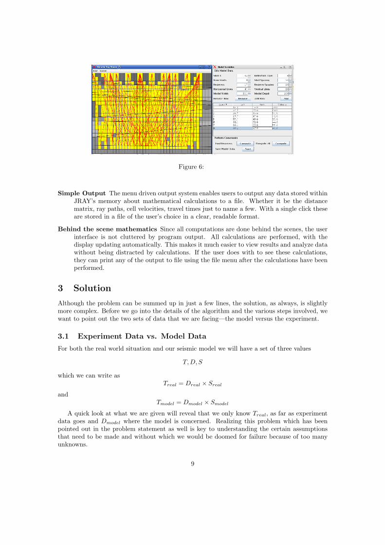
Figure 6:

Simple Output The menu driven output system enables users to output any data stored withinJRAY’s memory about mathematical calculations to a file. Whether it be the distancematrix, ray paths, cell velocities, travel times just to name a few. With a single click theseare stored in a file of the user’s choice in a clear, readable format.

Behind the scene mathematics Since all computations are done behind the scenes, the userinterface is not cluttered by program output. All calculations are performed, with thedisplay updating automatically. This makes it much easier to view results and analyze datawithout being distracted by calculations. If the user does with to see these calculations,they can print any of the output to file using the file menu after the calculations have beenperformed.

3 Solution

Although the problem can be summed up in just a few lines, the solution, as always, is slightlymore complex. Before we go into the details of the algorithm and the various steps involved, wewant to point out the two sets of data that we are facing—the model versus the experiment.

3.1 Experiment Data vs. Model Data

For both the real world situation and our seismic model we will have a set of three values

T,D, S

which we can write asTreal = Dreal × Sreal

andTmodel = Dmodel × Smodel

A quick look at what we are given will reveal that we only know Treal, as far as experimentdata goes and Dmodel where the model is concerned. Realizing this problem which has beenpointed out in the problem statement as well is key to understanding the certain assumptionsthat need to be made and without which we would be doomed for failure because of too manyunknowns.

9

The major assumption we need to make here is that our ray tracing has been accurate enoughin terms of the distances it has provided us with that we can consider the two distance matricesto be approximately equal. Thus we would have

Dreal = Dmodel = D

This is however not the only assumption we need to make as we will soon see in the first step ofthe proposed algorithm.

3.2 Algorithm

In order to calculate the value of Sreal, or a value close enough to it to be within an acceptableerror, the following algorithm has been proposed:

1. Estimate an initial value for Smodel. This new assumption can be based on the values usedin the ray tracing or can be chosen entirely at random, although the former would help fora faster convergence.

2. We can now calculate a provisional Tmodel = D × Smodel.

3. Having a value for Tmodel and the original Treal we can now compute the variation in traveltimes given by

∆T = Treal − Tmodel

4. After having calculated the variation in travel time we can subtract

Tmodel = D × Smodel

fromTreal = D × Sreal

which will give usTreal − Tmodel = D × (Sreal − Smodel)

∆T = D ×∆S

5. Solve ∆T = D ×∆S for ∆S and compute Sreal from it.

6. Re-evaluate Smodel = Sreal. The = in this case stands for assignment rather than itsarithmetic equality.

7. Reiterate Steps 2–6 until little or no variation can be observed between Smodel and Sreal.We will then have reached the most accurate values for the real slowness. The acceptableerror is given by ∆T as soon as its value drops under 0.001 milliseconds.

As part of this project, the above algorithm was implemented in the C programming language.The choice for C over a more convenient, mathematically-oriented programming language is dueto compatibility issues with OpenGL, the ability to create programming platform-independentbinary executables and a tighter integration with other applications.

10

3.3 The Least Square Problem

A quick scan over the algorithm presented in the previous section will reveal that the mostimportant step, both computationally but also as the key to the entire algorithm, is Step 5where a system of equations is solved. It should be noted at this point that in practice the raysfar outnumber the cells. While we have a number of rays of the order of 104, the number ofcells is usually of the order of 102. This leaves the system ∆T = D × ∆S in a state of beingover-determined. Since there is no exact solution this becomes a least square problem.

If we try to imagine the travel path of a ray through the cells it become fairly clear thatthe number of cells traversed by one individual cell is very low compared to the total number.This can lead us to conclude that every row in D has a very small number of elements that arenon-zero. By generalizing to the entire matrix we can conclude that D is a very sparse matrix.Practice confirms with approximately 99% of the elements in a distance matrix being zero. Thissituation allows us to rule out any attempt of solving the system with a QR decomposition.Instead we will employ the conjugate gradient method.

3.3.1 Conjugate Gradient

The method of conjugate gradient changes the problem of solving Ax = b into an equivalent one.For this purpose we consider the function φ(x) defined as

φ(x) =12xT Ax− xT b

where x ∈ Rn and A ∈ Rn×n. The minimum value of φ(x) is −bT A−1b/2 which is reached atx = A−1b. Thus the problem become finding the x for which φ(x) reaches its minimum. Theeasiest way to do this is to employ the steepest descent method.

The method of steepest descent starts from the statement that at a current point xc thefunction φ(x) decreases most rapidly in the direction of the negative gradient −∇φ(xc) = b−Axc.By calculating the residual of xc as rc = b−Axc we can pick values of x to further minimize φ(x)until the residual falls under a predetermined value. That is, if rc is not zero, we can concludethat there exists a positive α such that φ(xc + αrc) < φ(xc). When performing steepest descentwe set α = rT

c rc/rTc Arc thus minimizing φ(xc + αrc). A C routine to perform this algorithm

can be quickly programmed. The value we have chosen as a requirement for the residual beforeending the algorithm is 10−3.

As a remark we would like to point out that to apply a conjugate gradient algorithm, thematrix A is required to be positive definite. The matrix D is not positive definite but we canreplace it with

M = DT D

which is a non-negative definite matrix, albeit possibly having a zero eingenvalue.

3.4 Computational Issues

A very obvious computational issue results from a fact stated in a previous section regarding thelow number of cells any given ray will traverse. Since D is very sparse and made up of manyzeros, a lot of processor time can be wasted in Step 2 of the algorithm where D × Smodel iscomputed. The processor will waste a flop for every zero element of D which can be catastrophicfor a high number of rays and cells. To avoid this, instead of storing D it as classical matrix,we have decided to store it as tuples (d, i, j) where the d is the actual value that would reside inD[i.j]. We now only need to store non-zero elements.

11

To calculate Tmodel we now just compute every element as Tmodel[i] = ΣjdSmodel[j]. Althoughthe formula might look misleading it should be remarked that d differs between tuple and thesymbol d only refers to the distance value in a tuple in general and not to a specific value. Toperform the calculation we initialize Tmodel = 0. We then process the tuples one at a time andin each iteration we add the product dSmodel[j] to the corresponding element of Tmodel[i] givenby the i in the tuple. The same technique can be applied in Step 5 when calculating DT ×∆T .In this case though, by transposing, tuple (d, i, j) becomes (d, j, i).

Another computational issue that needs to be taken into account is to remember that Step5 is a least square problem. This means that the solution we will get in the end is one possiblesolution but by no means the only one. Least squares problems can have several solutions thatwill satisfy the original system. In general the solution we do get is close enough to the realvalue for the purposes of seismic tomography that this does not play a major role. Nonetheless,care should be applied to ray tracing. Minor errors here could ill-condition Step 5 and producewrong results.

4 Conclusions and Future Work

As we have pointed out earlier in this document, to be able to run the proposed algorithmand reach a correct result we need to have certain previous knowledge of where the reflectionboundaries are as well as have a general idea of the velocity parameters of the cells. This can bequite limiting and will only allow the algorithm to be used in order to further refine the slownessvalues for each cell. However, it seems that in reality we sometimes misplace reflection interfacesand that causes us to err significantly in determining the structure of the subsurface.

Imagine we think there is a boundary about 1-ft closer to the surface than it actually is.This means that in a time t the a ray reflecting on the respective boundary will travel a distanceapproximately 2-ft longer than what we traced. This would seem to suggest that since moredistance was covered in the same time the cells that were traversed have a lower aggregateslowness than we anticipated with our model. The algorithm will run in this case as well, and itwill produce results. However, they will not be refining the value of the real slowness vector butrather an imaginary situation.

To void being dependent on previous information regarding the subsurface in the future,the mathematical treatment of the problem can be refined, perhaps even introducing a conceptof probability regarding the location of a reflection boundary. This way, while running thealgorithm based on a more or less accurate assumption we would be able to start confirming ordisproving the placement of reflection boundaries by the effective use of probabilities. This couldalso allows us to introduce new boundaries that were not taken into account before but which thedata seem to indicate as possible. The end result will be a much more accurate approximationof the structure of the subsurface.

5 References

• Gadallah, M.R. Reservoir Seismology: Geophysics in Nontechnical Language. Tulsa, Ok-lahoma: PennWell Books, 1994.

• Golub, G.H. & Loan, Van, C. F. Matrix Computations. Baltimore, Maryland: The JohnsHopkins University Press, 1996.

• Tarantola, A. Inverse Problem Theory and Methods for Model Parameter Estimation.Philadelphia, Pennsylvania: SIAM, 2005.

12