transportation research part e - its news | institute … · selective vehicle routing ... network...

Transportation Research Part E 62 (2014) 68–88

Contents lists available at ScienceDirect

Transportation Research Part E

journal homepage: www.elsevier .com/locate / t re

Selective vehicle routing problems under uncertainty withoutrecourse

1366-5545/$ - see front matter � 2013 Elsevier Ltd. All rights reserved.http://dx.doi.org/10.1016/j.tre.2013.12.004

⇑ Corresponding author. Tel.: +1 416 979 5000x7618.E-mail addresses: [email protected], [email protected] (J.Y.J. Chow).

Mahdieh Allahviranloo a, Joseph Y.J. Chow b,⇑, Will W. Recker a

a Institute of Transportation Studies, University of California, Irvine, CA 92697, USAb Department of Civil Engineering, Ryerson University, Toronto, ON M5B 2K3, Canada

a r t i c l e i n f o

Article history:Received 24 February 2013Received in revised form 24 September 2013Accepted 4 December 2013

Keywords:Selective vehicle routing problemStochastic optimizationFuzzy optimizationReliabilityRobust optimizationParallel genetic algorithmHumanitarian logistics

a b s t r a c t

We argue that the selective vehicle routing problem is more appropriate than the conven-tional VRP in handling uncertainty with limited resources. However, previous formulationsof selective VRPs have all been deterministic. Three new formulations are proposed toaccount for different optimization strategies under uncertain demand (or utility) level: reli-able, robust, and fuzzy selective vehicle routing problems. Three parallel genetic algo-rithms (PGAs) and a classic genetic algorithm are developed and compared to thedeterministic solution. PGAs differ based on their communication strategies and diversityin sub-populations. Results show that a PGA, wherein communication between demes, orsubpopulations, occurs in every generation and does not eliminate repeated chromosomes,outperforms other algorithms at the cost of higher computation time. A faster variation ofPGA is used to solve the non-convex reliable selective VRP, robust selective VRP and thelarge-scale fuzzy selective VRP, consisting of 200 nodes. Large scale application demon-strates the value of fuzzy selective vehicle routing problem FSVRP in humanitarianlogistics.

� 2013 Elsevier Ltd. All rights reserved.

1. Introduction

The canonical vehicle routing problem (VRP) seeks the optimal route and distribution of vehicles to different nodes in thenetwork such that vehicles start their trips from the depot and return to the depot after serving all vertices in the network ina least cost manner. Different variations of vehicle routing problems have been introduced and applied to benchmark in-stances or real-world applications. Among these variations are models designed to deal with uncertain elements that canarise; for example, demand at nodes or travel time between nodes. In the past two decades, applications of these VRPs underuncertainty have gained increased interest both from researchers and practitioners due to two key factors: (1) the rise of realtime technologies that improve dynamic routing (Regan et al., 1996; Ghiani et al., 2003), and (2) the need for humanitarianlogistics and emergency response to devastating disasters (Sheu, 2007; Van Hentenryck et al., 2010; Bozorgi-Amiri et al.,2013; Chen and Miller-Hooks, 2012; Huang et al., 2012).

Given the large body of literature on uncertain routing applications, how appropriate are the assumptions used to moti-vate the studies? Optimization under uncertainty encompasses a broad spectrum of theories that include both stochastic andfuzzy variables (Liu, 2009). There are two general frameworks to handle uncertainty, depending on the availability of infor-mation. In the first category, information are obtained or updated over time, and optimal policies for sequential decision-making are determined (e.g. Chow and Regan, 2011a; Powell et al., 2012). Conventional Dantzig-esque two-stage stochasticprogramming with recourse can be considered a subcategory of the Bellman-esque dynamic programming methods, one

http://crossmark.crossref.org/dialog/?doi=10.1016/j.tre.2013.12.004&domain=pdf

http://dx.doi.org/10.1016/j.tre.2013.12.004

mailto:[email protected]

mailto:[email protected]

http://dx.doi.org/10.1016/j.tre.2013.12.004

http://www.sciencedirect.com/science/journal/13665545

http://www.elsevier.com/locate/tre

M. Allahviranloo et al. / Transportation Research Part E 62 (2014) 68–88 69

based on a myopic policy. Most stochastic or fuzzy routing problems deal with this first category with recourse (e.g. Gan andRecker, 2013).

The second category is where no recourse is possible—where the consequences of the decisions are much greater. It isassumed that the uncertainties related to nodes cannot be realized within reasonable time, and hard decisions need to bemade without recourse considerations. One primary example of this case is in large scale disasters, where relief organiza-tions need to race against the clock to provide limited supplies to a large region where the demand far exceeds the supply.By the time additional information is provided and can be of use, the number of casualties may have already escalated out ofcontrol. As noted in Van Hentenryck et al. (2010), a standard VRP solution that provides a route through all nodes is not avery practical solution in humanitarian logistics.

Although there are a growing number of studies dealing with this setting in which there should be no recourse, the firstcategory of uncertain routing models continues to be used even in those contexts. The contribution of this paper is to high-light this fallacy, and to show how it can be rectified in the form of new uncertain vehicle routing problem formulations andsolution algorithms for the case when the utility gained from visiting nodes is uncertain. Applications to simple and largescale networks are devised for consideration in humanitarian logistics, and to provide benchmarks for future improvements.

The remaining sections of the paper are as follows: Section 2 includes a literature review of uncertain vehicle routing andstrategies to deal with the uncertainty. Section 3 presents a motivational example for why the selective VRP is better suitedto deal with no recourse, and the formulation is formalized from various special cases proposed in the literature. Addition-ally, formulations of the selective vehicle routing problem under uncertainty are proposed for three strategies to resolveuncertainty: reliability maximization, robust optimization, and maximization of fuzzy importance values. In Section 4, dif-ferent parallel genetic algorithms are developed and their accuracies, computation times, and convergence trends are eval-uated. A parallel genetic algorithm is used to solve the non-convex problems and is also adapted to solve large-scaleinstances of the fuzzy problem. In Section 5, we benchmark the performances of the three selective vehicle routing problemformulations on a small test network. In Section 6, we apply our proposed fuzzy selective vehicle routing problem (FSVRP) toa 200-node network with the parallel genetic algorithm (PGA) to demonstrate the value of this approach in humanitarianlogistics, and Section 7 concludes the paper.

2. Literature review

2.1. Stochastic VRPs

VRPs with stochastic demand (VRPSD) have been studied for well over thirty years (Stewart and Golden, 1983). Nonethe-less, there have been great debates over how the solution of a selective vehicle routing problem (SVRP) should be inter-preted. Jaillet (1988) presented an analytical approach to solve the probabilistic traveling salesman problem (PTSP) as ana priori solution for recourse strategies, and Bertsimas (1988) extended that to VRPSDs. In their framework, the solution gen-erated in the first stage is an a priori solution that is evaluated in the recourse stage, and the objective is to minimize costs inboth stages. The assumption in their approach is that the solution to the VRPSD is not meant to be interpreted as a stand-alone final solution, but to be used as an a priori solution to speed up subsequent reoptimization in a sequential, dynamicrouting context (Bertsimas et al., 1990). Bertsimas (1992) presented two recourse strategies to further justify the need foran a priori solution: one where demand is only realized when a node is visited and one where demand is realized at the startof the day and where nodes with zero demand are omitted from the a priori sequence. Gendreau et al. (1996a) have provideda summary of the literature up to that point. Much of the more recent literature in this area either deals with solution algo-rithms (e.g. Gendreau et al., 1995, 1996b; Laporte et al., 2002; Kenyon and Morton, 2003; Bianchi et al., 2006; Tan et al.,2007; Moghaddam et al., 2012) or with different optimization objectives, as described below.

Instead of solving for the optimal expected solution, one optimization objective in uncertain programming is to maximizethe reliability that a solution will perform within a specified threshold. One example is to maximize the travel time reliabil-ity, which seeks a solution that maximizes the probability of the travel time being less than a certain threshold. In the con-text of humanitarian logistics, certain routes have a probability of having failed and suppliers need to consider routes thatare most reliable. This is observed in Kenyon and Morton’s (2003) formulation to maximize the probability of completing allvehicle tours within a given deadline. Reliability maximization is also quite common in other network problems. For exam-ple, Chen et al. (2007) applied a reliability method in a network design problem, where the problem is comprised of a two-stage optimization problem, with a chance-constrained travel time minimization problem as an upper-stage problem anduser equilibrium network problem as a lower-stage optimization model. For other examples of reliability objectives in trans-portation networks, readers are referred to Daskin and Hesse (1997), Ng and Waller (2009), and Ji et al. (2011).

A second optimization objective is robust optimization. Robust optimization seeks a solution that is resilient against dis-ruptions or other random events. For example, a robust distribution plan in humanitarian logistics would be the least sen-sitive to the probability of routes having failed. Unlike reliability maximization, robust optimization seeks a risk-aversesolution. A robust optimization problem can be formulated a number of different ways, one of which is to optimize the solu-tion under the worst case scenario. Ben-Tal and Nemirovski (1998) showed that such problems are tractable, while Sunguret al. (2008) solved a robust VRP optimizing the worst case scenario. Agra et al. (2013) proposed two formulations for the

70 M. Allahviranloo et al. / Transportation Research Part E 62 (2014) 68–88

robust VRP based on the linear approach. Li et al. (2012) proposed a different linear robust optimization model that also cap-tured the variance, and applied it to sustainable toll design.

Another solution to robust optimization is a mean–variance formulation that optimizes the expected value and mini-mizes the variance of the objective value as defined in Mulvey et al. (1995). Although this second approach is nonconvex,it provides a flexible multi-objective framework that allows decision-makers to adapt the degree of robustness of their solu-tion. For example, the mean–variance approach has been applied to network design problems (Chen et al., 2006; Yin, 2008;Chow and Regan, 2013) so that the robustness can be managed as a multi-objective problem. The mean–variance approachhas generally not been applied to robust VRPs.

2.2. Fuzzy VRPs

A third uncertain approach has been considered in VRPs: treating variables as fuzzy variables instead of stochastic vari-ables with known distributions. Fuzzy variables are more suited to scenarios with no recourse, since those circumstancesoften do not have known distributions (He and Xu, 2005). They can capture imperfect information during humanitarianoperations (Sheu, 2007, 2010). Given its importance to our treatment of uncertain VRPs without recourse, a brief introduc-tion to fuzzy sets and variables is provided.

Definition 1 (Fuzzy set). Unlike deterministic sets, where membership of a subject to a set can be represented by binaryvariables (0 representing non-membership and 1 representing membership), an instance in a fuzzy sets has a partialmembership value to the sets, (for example, membership of a person to the set of tall people being subject to non-preciseinterpretation of ‘‘tall’’).

If X is a set of objects represented by x, the fuzzy set of x is shown as eA, and is defined by:
eA ¼ fðx;leAðxÞÞjx 2 Xg ð1Þ
where eA, Fuzzy set; leAðxÞ, the degree of membership of x in eA. Generally, it is a normalized value in the range of 0 and 1(Zimmermann, 1996).

Definition 2 (Fuzzy number). Fuzzy numbers represent convex and normalized fuzzy sets. The value of membership of afuzzy number varies in the range of 0 to 1. Triangular, trapezoidal, and bell-shaped curves are the most commonly used fuzzynumbers in the literature. Triangular and trapezoidal fuzzy numbers are normally represented by their vertices (a1, a2, a3)and (a1, a2, a3, a4), respectively, as illustrated in Fig. 1.

Definition 3 (a-Level set). An a-level set of eA is a fuzzy set in which the membership value of every member is greater thanor equal to a. It is represented by the expression in Eq. (2).

Aa ¼ fx 2 XjleAðxÞP ag ð2Þ

Thus far, in all applications of fuzzy logic in vehicle routing problems, visiting every location is forced by the constraintset. The fuzzy concept is used either in computing the remaining capacity of the vehicle or in scheduling the visits. Teodo-rovic and Pavkovic (1996) solved a VRP with fuzzy demand. The problem is to minimize total cost with known locations andvehicle capacity, and approximate demand values. Teodorovic and Radivojevic (2000) used a fuzzy decision-making proce-dure to make a decision regarding whether a node with fuzzy demand should be assigned to the route or what the schedulewould be for the nodes in a Dial-a-Ride Problem route. Wang and Wen (2002) applied fuzzy time constraints in a DirectedChinese Postman Problem. Kuo et al. (2004) used an ant colony algorithm to solve a vehicle routing problem with both fuzzytravel time and time windows. He and Xu (2005) used a genetic algorithm to solve a VRP with probabilistic travel time andfuzzy demand. Zheng and Liu (2006) applied credibility measures of fuzzy values in constraints with the criteria that the

(a) (b)

Fig. 1. Triangular and trapezoidal representation of fuzzy numbers.


credibility measure should be higher than a predefined value, and used a genetic algorithm to solve the vehicle routing prob-lem. Tang et al. (2009) formulated the VRP with fuzzy time windows as a multi-objective problem. Gupta et al. (2010) solveda multi-objective VRP with fuzzy time windows using a genetic algorithm. Cao and Lai (2010) solved a VRP with fuzzy de-mand as a chance constrained optimization problem, where the credibility of the demand to be within a specific range has athreshold value. Xu et al. (2011) proposed a solution for VRP with fuzzy random time windows.

3. Selective VRPs (SVRPs)

In the following sections, we briefly argue for why SVRPs under uncertainty are more generalized cases of classical VRPsunder uncertainty; then we present the general formulation for the selective vehicle routing problem.

3.1. Motivating example

The conventional probabilistic TSP (PTSP), as presented by Jaillet (1988), finds an a priori route through all nodes, wherethe nodes have random binary demands. Consider the following simplified example of the PTSP, but assume that no recourseis available, as shown in Fig. 2.

There are two nodes with equal utility ‘u’ that can be attained by visiting them, three links of equal length c, and withindependent and identically distributed Bernoulli probabilities p (where q = 1 – p) of occurring. The PTSP is defined in sucha way that the only two possible routes (0-A-B-0 and 0-B-A-0) are equivalent solutions here, and are the only available solu-tions and strategies. The utility of either route is ‘2u – 3c’ if both nodes generate utility, but the situation can be worse off, asillustrated by the probabilistic outcomes in Table 1.

On the other hand, a selective or profitable VRP is a variant problem that allows a subset of nodes to be visited. Underthese circumstances, the value of having selection in the profitable tour approach can be clearly distinguished. The solutioncan be to make no visits, visit one of the nodes (either one due to symmetry), or visit both nodes (equivalent to the PTSPsolution). Obviously this adds flexibility to the set of solutions, and the value of that can be determined. No visits wouldbe made if the expected values of the other two options result in negative utility (the travel cost exceeds the expected profit).If only one node is visited, the utility (with expected utility of up – 2c) is

1 node ¼u� 2c; p

�2c; q

�
In terms of maximizing the expected value, assuming 2u > 3c (otherwise there would be no value to visiting the nodes at
all), the optimal strategy is to make no visits if p < 3c/2u (resulting in expected utility of 0) and to make two visits otherwise.The single node visit is dominated by the two-node visit under this criterion of maximizing expected utility. Nonetheless,introducing the option to make no visits improves upon the value of the strategies, as shown in Fig. 3 below. Having the op-tion to select nodes to construct a subtour introduces greater flexibility simply from a perspective of expected utility, trans-forming the PTSP solution (in red) to the dashed green solution in Fig. 3.

In the situation where there is recourse, such a static solution would have less value since it can be modified as new dataare obtained. We do not prove that a selective solution would be better than a non-selective solution in all cases, althoughfuture studies can consider this prospect. This example shows that having selection can add a flexibility premium to the net-work optimization solution without having to introduce a timing component, contrary to the redesign premium due todeferral discussed in Chow and Regan (2011b).

We consider the TSP with the understanding that the conclusions here naturally extend to VRP. The benefit does not endthere, as having more options allows for other objective criteria as well. Maximizing reliability can be considered for bothprobabilistic and fuzzy selective problems, while maximizing robustness can be considered for probabilistic problems.

Fig. 2. Motivating example network.

Table 1Probabilities and utilities of each option if all nodes visited.

Alternative Utility Probability

1: 2 nodes fail �3c q2

2: 1 node fails u � 3c 2pq3: 0 nodes fail 2u � 3c p2

Fig. 3. Expected utility of profitable tour approach (dashed green) compared to probabilistic TSP (solid red). (For interpretation of the references to colour inthis figure legend, the reader is referred to the web version of this article.)


3.2. Formulation for selective VRPs (SVRPs)

To the authors’ knowledge, all of the studies cited in Sections 2.1 and 2.2 require the solution to visit every node in thenetwork. Most importantly, the a priori solution approach assumes that recourse is possible. In many cases it is not possibleto obtain information for recourse (e.g., large-scale disaster relief where information is not readily available), and in suchcases the a priori solution of visiting every node would not be effective. One way to overcome this issue is to solve a selectiveVRP instead. In their selective traveling salesman problem paper, Laporte and Martello (1990) formulated the problem as aninteger program with the objective function of maximizing profit subject to upper-bound costs.

Feillet et al. (2005) provided a review of profitable TSPs where the utility of omitted nodes is minimized along with travelcost. When either the number of nodes to be visited or amount of total profit from a visited node is set as a constraint, theproblem is called a prize collecting traveling salesman problem. When the travel cost is constrained and the objective iseither to maximize the number of nodes to visit or the total profit from visited nodes, it is an orienteering problem. Chowand Liu (2012) proposed a generalized profitable tour problem in the context of traveler activity recommendations, whereusers would input desired activity types (e.g. Italian restaurant, a particular movie) into an online portal or mobile device andthe routing engine would find the optimal schedule and destinations, together with fuel constraint considerations, usingsuch online resources as Yelp. VRPs with selective pickup were also considered by Gribkovskaia et al. (2008). Valle et al.(2009) formulated a SVRP with an objective of minimizing the longest route. Chow (in press) proposed a selective extensionto Recker’s (1995) Household Activity Pattern Problem (HAPP), a variant of the pickup and delivery problem for assigninghousehold schedules. Allahviranloo and Recker (2013) modeled selective activity engagement within a household, using fuz-zy parameters. They employed fuzzy numbers as a tool to represent desirability of activities and solved a variation of selec-tive pickup and delivery problem. Their study is one of the first formulations of a variant of the SVRP dealing withuncertainty.

A mathematical programming formulation of the SVRP is provided for clarity. Depending on the utility gained from vis-iting nodes and other terms of the objective function, some of the nodes will be served in the system. Utility can be specifiedas the demand level at the node, importance of the node in the network, etc. In this paper, we use the importance of the nodeas a measure of its utility. The formulation of the SVRP in this paper is formalized from the earlier work cited above, whereprior instances were either profitable TSPs or such selective variants of VRP as the PDP and HAPP. Specifically, we considerthe multi-objective uncapacitated SVRP problem with time windows:

Min Z1 ¼Xm2V

Xi2P

Xj2P

ðcmij þ ctmijÞX

mij

Max Z2 ¼Xi2P

Ui

Xm2V

Xj2P

Xmij

ð3Þ


subject to:
Xm
Xj

Xmij 6 1; 8i 2 P; ð4ÞX

j

Xmij �

Xj

Xmji ¼ 0; 8i 2 P;8m 2 V ; ð5ÞX

j

Xm0j 6 1; 8m 2 V ; ð6ÞX

i

Xmi;nþ1 �

Xi

Xm0i ¼ 0; 8m 2 V ; ð7ÞX

i

Xmi0 ¼ 0; 8m 2 V ð8Þ

Ti þ Si þ tij � Tj 6 M � ð1� XmijÞ; 8i; j 2 N;8m 2 V ; ð9Þ

ai 6 Ti 6 bi; 8i 2 P; ð10Þ

where:� Ui: Perceived utility gained from visiting node.� Xm

ij: Binary decision variable takes the value of unity if vehicle v travels from node i to node j, and zero otherwise.� V = {1, . . ., v, . . ., |V|}: Set of vehicles.� P = {1, 2, . . ., n}: Set designating node locations.� N = {0, P, n + 1}: Set of all nodes, including those associated with the initial departure and final return to depot.� Ti; i 2 P: Time at which node i is visited.� tmij; i; j 2 N; m 2 V: Known travel time between nodes i, j by vehicle v.� cm

ij; i; j 2 N; m 2 V : Known travel cost between nodes i, j by vehicle v.� Si; i 2 P: Duration of service at location i.� ai; i 2 N: Earliest open time windows for location i.� bi; i 2 N: Latest open time windows for location i.� c: Monetary value of time.� M: Large number.

Here, Z1 is the objective of minimizing the total ‘‘cost’’ of travel, comprised of travel cost and travel time weighted bythe monetary value of time (for simplicity of presentation, in the following examples we use the explicit time valuerather than the ‘‘cost’’ of time, as represented by the value of travel time (e.g. Wardman, 1998; Lam and Small,2001); this is equivalent to assuming a value of c per unit time) and Z2 is the objective of maximizing utility gainedfrom visiting nodes. Constraints (4) require every node to be visited by at most one vehicle. Constraints (5) conservethe flow in the network; constraints (6) allow vehicles to stay in the depot; constraints (7) require all vehicles leavingthe depot to be back in the depot at the end of the service. Constraints (8) prevent a vehicle from returning to the start-ing origin. Constraints (9) require the arrival time to every location to be equal or greater than the sum of the arrivaltime to the previous location, service time at that location, and travel time between the two locations; these are effec-tively the subtour elimination constraints. Constraints (10) represent the time window constraints for each location.Since the arrival times of nodes that are not selected do not factor into the objective function, the time window con-straints can hold for every node i.

There are at least two examples of problems that benefit from formulation as a SVRP model under uncertainty. First, whenthere is a shortage of supply or when the total supply of the fleet cannot meet the demand level in the network, it may not befeasible to plan a set of routes through every single node—a large-scale disaster with a limited supply of rescue vehicles is areal-life example of this case. Second, when there are time limitations and some critical nodes need to be visited before itbecomes too late, an a priori route that selects a subset of nodes to visit can ensure that those nodes are visited in a timelymanner.

In this paper, we propose three formulations for different types of SVRP under uncertainty: the fuzzy SVRP (FSVRP), thereliable SVRP and the robust SVRP, when the utility is stochastic.

3.3. Selective vehicle routing problem under uncertainty without recourse

3.3.1. Fuzzy selective vehicle routing problem with time windows (FSVRPTW)In FSVRP, there is a corresponding importance value for visiting each node and the objective function includes minimizing

the sum of total travel time and travel cost in the network, and maximizing the utility gained from importance of visitingevery node. In our FSVRP formulations, the objective function in Eq. (3) used in the deterministic SVRP is replaced by its fuzzyequivalent, Eq. (11), with the same constraint set.


Min Z1 ¼Xm2V

Xi2P

Xj2P

ðcmij þ ctmijÞX

mij

Max Z2 ¼Xi2P

eIi

Xm2V

Xj2P

Xmij

ð11Þ

where eIi is the Fuzzy number representing the importance, or utility gained, of visiting node i.Fuzzy representation of the importance values works well in capturing uncertainty where the values are vague and un-

known to the decision maker. Different approaches have been proposed to solve optimization problems with fuzzy objectivefunctions, as noted in the literature review in Section 2.2. Zimmermann (1978) proposed a solution based on maximizingminimum importance value. Tong (1994) solved the problem by using interval optimization techniques. In this paper thelatter method is used for two reasons. First, it has a linear objective function, which makes it easier to solve. Second, basedon different levels of uncertainty, the method provides a spectrum of solutions to the problem.

If the importance of visiting any given node is a triangular fuzzy number as shown in Fig. 4, then we can cut its fuzzydiagram with any given a;0 6 a 6 1. Higher values of cutting level represent higher degrees of certainty. A cutting diagramfor different values of a will generate a -level sets, and for any given cut-level the corresponding set will be ½IaL;i; I

aU;i�. Using

this range, the formulation with fuzzy coefficients in the objective function, Eq. (12), is shown below.

Min Z1 ¼Xm2V

Xi2P

Xj2P

ðcmij þ ctmijÞX

mij

Max Z2 ¼Xi2P

IaL;i; IaU;i

h iXm2V

Xj2P

Xmij

ð12Þ

subject to:Constraints 4 to 10.The lower bound Za

L ¼ ðZ1; Za2LÞ and upper bound Za

U ¼ ðZ1; Za2UÞ of problem (12) can be obtained by solving the following

two linear problems (13a and 13b):

Min Z1 ¼Xm2V

Xi2P

Xj2P

ðcmij þ ctmijÞX

mij

Max Za2L ¼

Xi2P

IaL;iXv2V

Xj2P

Xmij

ðaÞ

Min Z1 ¼Xv2V

Xi2P

Xj2P

ðcmij þ ctmijÞX

mij

Max Za2U ¼

Xi2P

IaU;iXv2V

Xj2P

Xmij

ðbÞ ð13Þ

both subject to constraints (4)–(10), described above.By setting the importance of nodes to the lower/upper bound, the lower/upper bound of the objective function and the

corresponding solution is obtained. The problem is solved as two deterministic optimization problems to define the range ofthe lower and upper bounds of the fuzzy problem, dependent on the a. The resulting values of objective function and solu-tion will vary across the ½Za

L ; ZaU � and ½Xa

L ;XaU � intervals.

3.3.2. Reliable selective vehicle routing problem (RSVRP)The second model proposed is a reliable selective vehicle routing problem (RSVRP). The model is specified in terms of a

multi-objective function of minimizing total travel cost (comprised of actual cost plus value of time cost) and maximizingthe cumulative utility, g, that can be achieved with a predefined likelihood of success R, where

Pi2PUi

Pm2V

Pj2PXm

ij P g, asshown in Fig. 5. For example, if 1 – R = 95%, it is interpreted as the selection of nodes to visit such that the utility can bereached R = 5% of the time, which should result in a higher value of g than a more risk averse 1 – R = 75% which requires util-ity that can be achieved R = 25% of the time. While the deterministic equivalent approach is based on chance-constrainedliterature (e.g. Liu, 2009), this formulation is unique because the problem is specific to node selection.

The optimum solution to RSVRP is obtained through the following set of equations:

Min Z1 ¼Xm2V

Xi2P

Xj2P

ðcmij þ ctmijÞX

mij

Max Z2 ¼ gð14Þ

Fig. 4. a-Cut representation of a triangular fuzzy number.

Fig. 5. Illustration of utility distribution for Reliable Selective VRP (RSVRP).


subject to:

PrXi2P

Ui

Xm2V

Xj2P

Xmij P g

!P 1� R; and ð15Þ

constraints (4)–(10).Assuming utility of node i is distributed normally with mean of li and variance of ri Eq. (15) can be transformed to Eq.

(16). We can rewrite the RSVRP problem in Eqs. (14) and (15) as the same objectives with equivalent constraint in Eq. (16).

Min Z1 ¼Xm2V

Xi2P

Xj2P

ðcmij þ ctmijÞX

mij

Max Z2 ¼ g

subject to:

g�Xi2P

li

Xm2V

Xj2P

Xmij

!6 /�1ð1� RÞ:

ffiffiffiffiffiffiffiffiffiffiffiffiffiffiffiffiffiffiffiffiffiffiffiffiffiffiffiffiffiffiffiffiXi2P

r2i

Xm2V

Xj2P

Xmij

s; and ð16Þ

constraints (4)–(10).In equation (16), a location that is selected would contribute its utility to the sum, and any that are not visited would have

a zero mean and variance. This transformation converts the chance constrained problem to an equivalent deterministic non-linear programming problem and its solution can be found for a predetermined value of R, using parallel genetic algorithm(PGA_1), discussed in Section 4.

3.3.3. Robust (mean–variance) selective vehicle routing problem (MVSVRP)We formulate the robust selective vehicle routing problem as a mean–variance problem (MVSVRP) under different inde-

pendent scenarios for utility at each node (Fig. 6), where the probability of each scenario S is represented by pS and IiS denotes

the utility gained from visiting node i under that scenario.Assuming parameter b as the weight for the mean value of scenarios, the optimization problem is shown as the following

set of equations:

Min Z ¼ bX

S

pSfS þ ð1� bÞX

S

pSðfS � �f SÞ2 ð17Þ

subject to:

fS ¼Xm2V

Xi2P

Xj2P

ðcmij þ ctmijÞX

mij �

Xi2P

IiS

Xj2P

Xm2V

Xmij; and ð18Þ

constraints (4)–(10). MVSVRP has a nonlinear and non-convex objective function and similar to RSVRP, parallel genetic algo-rithm is developed to find the optimum solution. The details of the algorithm are explained in Section 4.

4. Parallel genetic algorithm

There have been only a few GAs designed for routing problems with the selective property: Tasgetiren and Smith (2000)for an orienteering problem, Chow and Liu (2012) for the generalized profitable tour problem, and Chow (in press) for theselective variant of the HAPP model. To further improve on these algorithms, we consider the use of parallel GAs (PGAs). A

Fig. 6. Discretizing utility distribution to generate various scenarios.


PGA searches a feasible region for the optimum solution by initiating different initial populations in each deme or subpop-ulation. According to Cantú-Paz (1998), PGA has a higher efficiency compared to classic GA methods. PGA has been applied toa number of vehicle routing problems in the literature. Ochi et al. (1998) used a hybrid parallel genetic algorithm to solveVRP with heterogeneous fleet. They applied petal decomposition to construct chromosomes; in petal decomposition, routesare in petal structure to form a flower and the best flower is found by sweeping nodes. Communications between parallelGAs occur when the percentage of replacement of parents with children is less than 5% or when the main modules are capa-ble of finishing. Berger and Barkaoui (2004) used a hybrid parallel genetic algorithm to solve a VRP with time windows con-straints. In their formulation, two populations with different objective functions are evolved in parallel. The first populationgenerates solutions by minimizing the travel distance, while the second finds the optimum solution with minimum violationof time windows. Ho et al. (2008) solved a multi-depot VRP with a hybrid GA. They demonstrated a hybrid GA where its ini-tial population is generated using the Clarke and Wright savings method and where the nearest neighbor dominates the casewith a random initial population.

In this study, three different PGA structures are tested and compared in terms of their efficiencies in convergence, com-putation time, and value of optimum solutions. Table 2 presents the underlying structures of the GAs developed for thestudy. As pointed out by Gendreau et al. (1996a,b), such simple algorithms for deterministic cases as Clarke and Wright sav-ings method do not work well alone for stochastic VRPs without some substantial modification, so we avoided comparingwith those algorithms since it would not provide much insight.

As shown in Table 2, scenarios are built based on two main criteria: ‘communication strategy’ and ‘elimination’.Two different communication strategies are compared. In Strategy 1, in every deme the initial population is evolved sep-

arately until it converges to local optima, then all populations in every deme are aggregated to make the final population toimplement another GA on top of the aggregated population (PGA_1). This is a variation of the hybrid PGA discussed in Cantú-Paz (1998). In Strategy 2, at every iteration, the best chromosome of each deme is copied to all other demes, replacing theworst chromosomes (PGA_2, PGA_3). In this strategy, communication occurs at every iteration.

The binary nature of the VRP and limiting constraints causes some chromosomes to appear in the solution set more thanonce after only 4 or 5 initial iterations of evolution. In order to speed up the computation, repeated solutions are eliminatedfrom the population at each iteration. The simulation stops when either the number of iterations exceeds a maximum or thepopulation size becomes less than the minimum population size defined for the problem. Although the elimination of re-peated solutions in PGA_1 and PGA_2 results in populations that are not as diverse as those in PGA_3, the strategy speedsup the computation.

Every evolution includes a crossover and a mutation step, where the details are as following:Crossover

� Select a random number, Pc.� For every chromosome i in population, generate a random number ui, if ui 6 Pc , add chromosome i to crossover pop-

ulation Popcr. Length of each chromosome equals to the number of nodes and each cell takes the value of 1 if the nodeis visited by any vehicle.

� Select two chromosomes (V1, V2) randomly from Popcr and cross them over to generate children (Liu, 2009). Thecrossover equations are as follows, where c is a random number:

Ch1 ¼ cV1 þ ð1� cÞÞV2

Table 2Genetic algorithms structures.

Name Multipledemes

Communication Eliminaterepeatedchromosomes

Classic geneticalgorithm (GA)

No n/a No

Parallel geneticalgorithm1(PGA_1)

Yes Communication occurs at the end, after all chromosomes converge to their local optima Yes, at the end ofevery iteration


Yes Communication occurs at every iteration and the best chromosome of each deme is copiedto all other demes, replacing worse chromosomes

Yes, at the end ofevery iteration


Yes Communication occurs at every iteration and the best chromosome of each deme is copiedto all other demes, replacing worse chromosomes

No

Table 3Algorithm performance comparison for small network.

Algorithm Number ofgenerations

Initialpopulationsize

Numberof demes

Value of objective functionfor the best solution

Average of optimumvalues for 10 simulation

Error(%)

CPUrunningtime

Numberof cores

GA 100 25,000 1 �53.30 �53.01 5.6 03:23:53 1PGA_1* 100 150,000 60 �53.85 �52.78 4.7 00:01:07 12PGA_2* 100 150,000 60 �54.23 �53.48 4.0 00:01:54 12PGA_3* 100 60,000 20 �56.44 �56.44 0.1 00:13:39 12

⁄ Parallel computation is executed using parallel computation toolbox in Matlab 2011b; the standalone executable files use 12 cores to run the simulation.These file are uploaded to the cluster computers and the CPU time is the cumulative processing time used by all cores. These times vary depending on theproperties of processing cores, task loads on cores, and number of cores. (For PGA_1, the total process time consumed by all cores to obtain final solution is67 s.)


Ch2 ¼ ð1� cÞÞV1 þ cV2

� Check the feasibility of children and calculate the value of objective function for children, F_Chld.The solution is infea-sible if the visit occurs out of available time windows. The visit order is randomly generated.

� Generate a random number, r. If r > 0.2 and the value of objective function for children are better than the worstparents in the population, replace parents with children.

Mutation

� Select a random number, Pm.� For every chromosome i in population, generate a random number u0i, if u0i 6 Pm, add chromosome i to mutation pop-

ulation Popm.� Select a chromosome for the mutation population and mutate it by generating a random vector d (Liu, 2009). The

mutation equation is as follows: Ch = Vi + d.� Check the feasibility of the solution and compute the value of objective function.� If a mutated child is better than the worst case in the population, replace the worst case with the child.

4.1. Algorithm comparison for a small network

In this section a comparison between different proposed algorithms, as discussed in Table 2, for a small network, underthe fuzzy selective vehicle routing formulation are presented. The small network consists of 15 nodes and 2 vehicles. Table 3illustrates the results obtained from the different algorithms. In this table, the corresponding error is estimated by compar-ing their objective functions to the value of the objective function for the exact solution, which is solved in GAMS22.2 for thesmall network instance. GAMS uses the commercial CPLEX solver to find the optimum solution. The value of the objectivefunction for the exact solution, computed in GAMS, is -56.491.

According to the results shown in Table 3, on average PGA_3 finds the best solution with the minimum error of 0.1%.However, it has the highest computation time compared to the other parallel algorithms and the classic genetic algorithmhas the highest computation time among all of the algorithms tested. This is mainly due to two reasons: first, for parallelalgorithms, we execute the code on 12 parallel cores. Second, the elimination strategy applied to PGA_1 and PGA_2 speedsup computation. As an example for the case of PGA_1, since we are using 12 cores, twelve demes (out of 60 demes) are

0 10 20 30 40 50 60 70 80 90 100

-56

-54

-52

-50

-48

-46

-44

Iteration Number

Objective function Obtained by GA, Small Network

0 10 20 30 40 50 60 70 80 90

-56

-54

-52

-50

-48

-46

-44

Iteration Number

Objective function Obtained by PGA1,Small Network

0 10 20 30 40 50 60 70 80 90 100

-56

-54

-52

-50

-48

-46

-44

Iteration Number


0 10 20 30 40 50 60 70 80 90 100

-56

-54

-52

-50

-48

-46

-44

Iteration Number


Fig. 7. Comparing convergence trend for the objective function in small network. (*Multiple colors for PGA cases represent different demes of PGA, startingwith different initial population and converging to a common solution after some iterations.)

Table 4Algorithm performance comparison for large network.

Algorithm Number ofgenerations

Initial populationsize

Number ofdemes

Value of objectivefunction

CPU runningtime

Number ofcores

GA 50 8000 1 �348.38 32:08:08 1PGA_1 100 150,000 20 �359.16 02:34:28 12PGA_2 100 150,000 20 �360.11 04:25:43 12PGA_3 100 60000 20 �364.878 28:16:56 12


initiated simultaneously with a randomly generated population of 7500. In the second generation, before generating thepopulation, the existence of repeated solutions is checked, and the repeated solutions are eliminated from population. Aftersome initial generations, population size in every deme decreases and this results in time savings. PGA_3 does not eliminaterepeated solutions so its computation time is greater than PGA_1 and PGA_2, but since it uses 12 cores, it is faster than theclassic GA. Even if the GA code is modified to use multiple cores, the performance of all four algorithms will improve and thecomputation time difference between algorithms will lessen, but PGA algorithms will still dominate GA since this piece ofcode is common among all algorithms. A comparison of algorithms on 10 randomly generated instances is included in theappendix under Table A1 along with the properties of input parameters in Table A2. For all 10 instances, PGA_3 finds the bestsolution with the minimum error.

Fig. 7 illustrates the convergence trend in the best solution of all algorithms. PGA_1 and PGA_2 converge to the local min-imum in early stages, 45th and 10th iteration, respectively. However, the classic Genetic Algorithm and PGA_3 require moregenerations to converge (around 60). In these algorithms, it is the tradeoff between simulation time and accuracy thatdesignates the best algorithm to implement.

4.2. Algorithm comparison for a large network

A similar comparison is made with a larger network consisting of 200 nodes and 20 vehicles; the results are shown inTable 4 and Fig. 8. For the large network, PGA_3 also outperforms the other algorithms at the cost of a longer computationtime.

Fig. 8 illustrates the change in the value of optimum objective function at each iteration. As shown in the figure, theclassic GA fails to search the feasible region properly, similar to the results obtained for the small network. It evolves over


a limited number of generations, and then converges to a solution, which is dominated by solutions obtained from the par-allel cases. Additionally, the computation time for an initial population of only 8000 is 10 times more than the computationtime for populations of 150,000 in PGA_1 and PGA_2 cases, since parallel algorithms operate on 12 cores.

Among all methods, PGA_3 finds the best solution, but its long computation time is a major drawback. Comparing thevalue of objective function and computation time for all four algorithms, PGA_1 has the lowest computation time. Comparedto PGA_1, PGA_2 improves objective function by 0.2% with 70% increase in computation time, and PGA_3 improves solutionby 1.6% with 10 times increase in computation time. Therefore, PGA_1 is employed to solve the reliability and robustexamples in Section 5, and the large network application in Section 6.

5. Evaluation of selective models under uncertainty

We apply the different SVRP models to a small network, consisting of 15 nodes and 2 vehicles. Due to the limited numberof vehicles and time windows constraints, a visit to every node is not feasible, so conventional VRPs under uncertainty wouldnot work for this test problem at all. Solutions for FSVRP are found using exact algorithms in GAMS. However, for RSVRP andMVSVRP we solve the nonconvex optimization problems using the PGA_1 discussed in Section 4. For the sake of brevity, thetravel time and travel cost in the network, fuzzy trapezoidal importance graphs, service duration and time windows for eachnode in the network, importance values for RSVRP and parameters of MVSVRP are appended to the paper as Tables A3–A6,Figs. A1 and A2.

5.1. Results of FSVRP on small network

Assuming 3 cut points for a-cut method to be 0, 0.5 and 1, the following exact solutions are obtained using GAMSprogramming software and shown in Fig. 9.

Fig. 9 illustrates the routing of two vehicles for different values of uncertainty. In this figure, the horizontal axis indicatestime of day and the vertical axis represents different scenarios for the value of uncertainty (i.e. cut-point) and simplifiedtransitions between chosen nodes in the tour. Relative travel times between two nodes are indicated by the non-horizontallines connecting two nodes, and flat lines denote time spent at a node. As an example, for the case when a = 1 at its lowerbound, vehicle 1 is dispatched to nodes 1, 9, 10, 5, and 3 at 07:15, 10:45, 13:30, 18:15 and 21:45.

Increasing the value of the cut point from 0 to 1 changes the optimum routes in the lower bounds and upper bounds to-ward a single solution. Despite the differences in the visiting order of nodes for different values of cut-points, some nodes arealways visited regardless of the value of cut-points. Table 5 shows the nodes that are visited together with travel cost, traveltime and total utility gained from visiting nodes.

Based on the results provided in Table 5, nodes 1, 2, 3, 4, 5, 9, 10 and 12 are visited in all optimal-route solutions, whereasnodes 11 and 14 are not part of the optimum route in any solution. That some nodes appear in the optimum route regardlessof the value of uncertainty provides valuable insight and can be a helpful tool in the decision-making process for cases inwhich there is a shortage in supply and there is no time to gather more information for recourse.

5.2. Results of RSVRP on small network

Fig. 10 illustrates the optimum routes obtained for the reliability methods under a 5% and 25% confidence level andTable 6 presents the values of different terms of the objective function for the reliable SVRP. It is assumed that importancevalues have a normal distribution with the mean and variance as reported in Table A5 of the appendix.

Two conclusions can be drawn from these results. First, the RSVRP works as intended, as the value of g that can beachieved diminishes from 71.14 to 66.01 as the confidence increases from 5% to 25%. A decision-maker who is more riskaverse will have to give up the higher maximum probabilistic utility that can be achieved. Second, the routes change be-tween these two solutions as well (intermediate value of 1 – R = 75% did not exhibit any change from 95%), showing thethreshold where higher risk aversion leads to swapping out Node 13 for Node 14 (the less risky choice).

5.3. Results of MVSVRP on small network

For the MVSVRP, we created six different scenarios, each with different importance values, as shown in Table A6 in theappendix. Assuming equal probability for each scenario, pS = 1/6, the following results in Fig. 11 are obtained.

Table 7 demonstrates the results of MVSVRP for the various values of b. For consistency reasons, PGA_1 is employed tofind the best solution.

The solutions make intuitive sense. As the criterion of minimizing mean at the expense of maximizing variance, b in-creases from b = 0 to b = 1 and as result the mean value improves from �46.60 up to �58.27 while the variance increasesfrom 9.59 up to 184.56. The visited nodes also change. As the importance of variance decreases, Node 2 is initially droppedin favor of Node 9, but when none of the weight is allocated to variance, Node 2 is brought back along with Node 4, Node 8,and Node 14.

0 5 10 15 20 25 30 35 40 45 50-370

-360

-350

-340

-330

-320

-310

Iteration Number

Objective function Obtained by GA,Large Network

0 5 10 15 20 25 30 35 40-370

-360

-350

-340

-330

-320

-310

Iteration Number

Objective function Obtainedby PGA1,Large Network

0 10 20 30 40 50 60 70 80 90 100-370

-360

-350

-340

-330

-320

-310

Iteration Number

Objective function Obtained by PGA2,Large Network

0 10 20 30 40 50 60 70 80 90 100-370

-360

-350

-340

-330

-320

-310

Iteration Number

Objective function Obtained by PGA3,Large Network

Fig. 8. Comparing convergence trend for the objective function in large network.

Fig. 9. Optimum patterns for visiting nodes at different a-levels.


Table 5Summary of fuzzy SVRP on small network.

Cut-point Nodes Cost Travel time Gained utility

1 2 3 4 5 6 7 8 9 10 11 12 13 14

a = 0, Low level 1 1 1 1 1 1 – – 1 1 – 1 1 – 1.179 4:00 54.25a = 0, Up level 1 1 1 1 1 1 – 1 1 1 – 1 – – 1.617 3:58 76.00a = 0.5, Low level 1 1 1 1 1 – 1 1 1 1 – 1 1 – 1.191 3:47 56.87a = 0.5, Up level 1 1 1 1 1 1 1 – 1 1 – 1 – – 1.357 5:02 72.25a = 1, Low level 1 1 1 1 1 1 – 1 1 1 – 1 – – 1.759 4:19 62a = 1, Up level 1 1 1 1 1 1 – 1 1 1 – 1 – – 1.759 4:19 71.5

Fig. 10. Reliable SVRP results on small network.

Table 6Reliable SVRP on small network estimated by PGA_1.

Description Visited nodes Cost Travel time (hh:mm) g

RSVRP, 1 – R = 95% 1, 2, 3, 4, 5, 8, 9, 10, 12, 13 1.07 3:40 71.14RSVRP, 1 – R = 75% 1, 2, 3, 4, 5, 8, 9, 10, 12, 14 1.16 03:42 66.01

Fig. 11. Robust MVSVRP results on small network.

Table 7Robust MVSVRP on small network estimated by PGA_1.

Description Visited nodesP

SpSfSa P

SpSðfS � �f SÞ2

bP

SpSfS þ ð1� bÞP

SpSðfS � �f SÞ2

Robust SVRP, b = 1 1, 2, 3, 4, 5, 8, 9, 12, 13, 14 �58.27 184.56 �58.27Robust SVRP, b = 0.5 1, 3, 5, 9, 10, 12, 13 �47.04 9.81 �18.61Robust SVRP, b = 0 1, 2, 3, 5, 10, 12, 13 �46.6 9.59 9.59

a fS ¼P

m2VP

i2PP

j2Pðcmij þ ctmijÞX

mij �

Pi2PIS

iP

j2PP

m2V Xmij .


In all three formulations of SVRP, there are certain parameters that need to be identified by decision makers: fuzzy impor-tance graphs and location of cut-point in FSVRP, reliability value in RSVRP, and the weight of mean and variance in MVSVRP.

Table 8A comparison of FSVRP, RSVRP, and MVSVRP.

Pros Cons

FSVRPLinear objective function, easy to extend Depending on the values of alpha, solutions varyDoes not need too much information regarding the distribution of

the uncertaintyFor every level of uncertainty, only 2 bounds are solved

Can be extended to larger examples and still provide good solutionsin reasonable time

For a small number of cut-points, analysis is reduced to only solving twodeterministic cases and does not cover the range of possible values for utility

RSVRPProvides an analytical representation between multiple random

distributions and a desired level of confidence in solution qualityNonlinear terms in the formulation results in high computation costsDistribution of uncertainty is requiredSome assumptions are needed to be made for reliability levelNot easy to extend to larger networks

MVSVRPProvides a robust solution by incorporating mean and variance of

different scenarios in the objective functionNonlinear terms in the formulation results in high computation costsDistribution of uncertainty is required

Multiobjective function allows for flexibility in managing degree ofrisk aversion

Some assumptions are needed to be made for scenario creationNot easy to extent to larger networks


Because of the different input parameters, it is not appropriate to compare the three sets of results presented here. Instead,the purpose is to verify the models, benchmark results for small instances for future replications, and to demonstrate theiruses. As all three models indicate, the ‘‘selection’’ characteristic leads to solutions that not only different in sequence andtiming, but also in nodes visited. This characteristic makes these problems very different from conventional stochastic VRPs.

Table 8 summarizes the general drawback and benefits associated to these models. In terms of finding an appropriate for-mulation or optimization strategy to employ, it depends on the nature of the problem. In Section 6, a fuzzy strategy is eval-uated in the context of humanitarian logistics.

6. Application of fuzzy selective vehicle routing problem to humanitarian logistics

According to EM-DAT, in 2011, natural disasters (earthquake, storm, draught, flood, volcano and wildfire) killed 30,216people and affected the lives of more than 254 million individuals around the world. The estimated total damage exceeded365 billion US dollars. Improving relief operations and dispatching equipment on-time to affected locations can reducepost-disaster casualties and shorten recovery duration. Relief logistics networks often require establishing repositories ordistribution nodes, called Points of Distribution (FEMA/USACE, 2008). More importantly, there are different types of logisticsnetworks for distributing supplies to affected regions, depending on the types of social networks present in the area: AgencyCentric Efforts, Partially Integrated Efforts, and Collaborative Aid Networks (Holguín-Veras et al., 2012). In other words, thestructure of a region’s social knowledge on perceived importance of different nodes can play a major factor in identifying thetype of logistics network to apply.

Due to the shortage in supply resources and uncertainty regarding priority of different nodes of the network as well theirdemand level, visiting every node in the network is impossible and may result both in a waste of supply as well as additionaldelay in serving the critical nodes of the network. However, based on the information about the distribution of the impor-tance of different nodes after the disaster, FSVRPs can be applied to exploit this information (such as the local social networksdescribed by Holguín-Veras et al., 2012) to identify the optimum network topology for delivering relief supplies.

In this section, we solve the FSVRP for a large network comprising 200 locations, which are randomly generated over anarea of 50 � 50 square miles, with a fleet size of 20 vehicles for the system. Driving speed is assumed to be 35 mph, andEuclidean distances between nodes are used. Duration of service is generated from a normal distribution with the meanof 5.5 h and variance of 2 for this sample instance, the minimum and maximum durations are 1.34 and 10.78 respectively.

Membership Value

1

0.5 1 1.5 2 2.5 3 3.5 4 4.5 5 5.5 6 6.5 7 7.5 8 8.5 9 9.5 10

Fig. 12. Range of fuzzy importance graphs for humanitarian logistic network.

Fig. 13. Results of fuzzy SVRP in large network.


Fuzzy importance values vary in the range of 0 to 10. The single depot is located at (0, 0). For this study we only examine asingle depot problem, but the conclusions drawn from here regarding node stability and certainty-dependent ranges of routeattributes should be extendable to multiple depot variations.

Prior to solving FSVRP, we solve the deterministic case of visiting all nodes with the 20 vehicles, assuming that there areno time window constraints, to determine the worst-case tour length. The minimum time to serve all the nodes is found tobe 81 h and 30 min. Clearly, if the goal is to serve important nodes within the first 24 h after disaster occurs to ensure victims


can be aided in a timely manner, a solution that visits every node is infeasible. Furthermore, such a solution would be uselessif no additional information can be obtained to update the relief effort within that 24-h period. Given these reasons, we usethe FSVRP to identify the optimum dispatch scenarios.

Triangular fuzzy importance values are assumed for this example, as shown in Fig. 12. These graphs are preset importancegraphs that decision makers have in mind. As an example, suppose the value of importance for a given node is ‘4.2’, thendecision maker maps ‘4.2’ to the graphs in Fig. 12 and finds the graph(s) that ‘4.2’ belongs to, the corresponding corners,which are used for FSVRP, for 4.2 are [2.5, 4, 5.5]. If the importance value belongs to more than one set, the corners of fuzzynumbers are updates using corresponding expected value (Shapiro, 2009).

In this example we use the PGA_1 algorithm to find the optimal route for its short computation time and acceptable accu-racy. For each cut-point we execute PGA_1 with 250 demes, each deme with a population size of 1000. The computation timewas about 13 h for 5 scenarios (2.6 h per scenario), in i7 processor with quad cores and 2.3 GHz of CPU. This time is likely tobe shorter if re-coded and compiled in C++ for implementation in pre-disaster planning or if it runs with more parallel cores.Fig. 13 shows the results of FSVRP for different values of cut-points. In these sets of figures, blue dots show the location of thenodes. Comparing upper bounds and lower bounds of each cut-point, more nodes are visited in the upper bounds than thelower bounds. Fig. 13(f) demonstrates the priority of the nodes being visited. The larger circles indicate the set of nodes thatare selected for all degrees of uncertainty.

In a relief effort that is integrated with the local social network as suggested by Holguín-Veras et al. (2012), the degree ofimportance of different nodes can represent a fuzzy perception of social network hubs. The solution of the FSVRP provides aninformative canvas of which nodes should be targeted as PODs for distribution—under all degrees of uncertainty, they re-main stable solution points. In other words, one effective way to incorporate local social networks into relief efforts inhumanitarian logistics under uncertainty is to capture the social network hubs using fuzzy variables and to solve an FSVRPto identify PODs for routing a fleet of vehicles.

The results in Fig. 13 provide several insights. As alpha increases from zero to one, the range of number of vehicles to bedeployed changes from 17 to 20 vehicles down to 19 vehicles. The range of number of nodes that are visited also narrowdown in range from 72 to 101 nodes when alpha = 0 to 94 nodes when alpha = 1. Other similar comparisons can be madewith the importance values, travel times, and costs.

As the ranges change with the alpha’s, we can see the choice of nodes to visit also change in some cases, as we can seefrom examining the upper bound graphs from alpha = 0 to alpha = 0.5. We identify the nodes by the number of times theyare selected amongst these solutions to identify those that are more stable than other points. A clear subset of nodes emerge(the ones that occur in all five solutions, shown in red in the lower right corner of Fig. 13) as stable nodes that are included inevery route regardless of the degree of certainty that we have of their importance. In this example, it turns out a large num-ber of these nodes are present in the southern quadrant of the region, with a lone node in the northern quadrant. These nodesare likely to play a prominent role if decision-makers are unable to ascertain the degree of certainty in their informationduring a time of crisis.

Table A1Comparing algorithms on 10 randomly generated instances.

Instances Number of nodes Exact solution GA PGA_1 PGA_2 PGA_3

1 12 �72.14 �71.96 �71.96 �71.99 �71.992 10 �62.109 �61.53 �61.53 �61.53 �61.533 15 �85.02 �83.008 �83.126 �84.137 �84.294 13 �98.54 �97.30 �96.99 �96.53 �98.175 11 �56.15 �56.08 �56.08 �56.04 �56.086 11 �72.28 �71.99 �71.99 �71.99 �71.997 9 �51.16 �50.31 �50.31 �50.31 �50.318 14 �82.732 �80.84 �80.91 �80.65 �81.249 8 �53.104 �52.51 �52.51 �52.51 �52.51

10 16 �117.032 �112.07 �109.89 �113.70 �116.41

Membership Value

1

1.5 2 3 3.5 4.5 5 6 6.5 7.5 8 9 9.5 100.5

Fig. A1. Fuzzy importance graphs.

a b c d

Fig. A2. Probability distribution of importance.

Table A3Travel time (minutes) and travel cost ($) in hypothetical network.

Node 0 1 2 3 4 5 6 7 8 9 10 11 12 13 14

0 0 16 55 12 42 18 47 56 54 5 6 31 54 18 44(0.00) (0.09) (0.05) (0.07) (0.23) (0.11) (0.27) (0.08) (0.06) (0.05) (0.06) (0.15) (0.03) (0.09) (0.44)

1 16 0 39 27 34 23 31 40 45 12 17 17 23 8 39(0.09) (0.00) (0.22) (0.15) (0.18) (0.12) (0.18) (0.22) (0.23) (0.07) (0.09) (0.09) (0.25) (0.05) (0.42)

2 55 39 0 63 33 51 29 5 32 50 53 24 12 37 39(0.05) (0.22) (0.00) (0.09) (0.18) (0.28) (0.17) (0.03) (0.17) (0.28) (0.29) (0.15) (0.07) (0.21) (0.43)

3 12 27 63 0 44 16 58 65 56 15 11 39 60 26 44(0.06) (0.14) (0.34) (0.00) (0.24) (0.10) (0.08) (0.38) (0.07) (0.07) (0.06) (0.23) (0.34) (0.17) (0.49)

4 42 34 33 44 0 27 50 37 13 37 36 22 23 27 6(0.21) (0.19) (0.17) (0.24) (0.00) (0.16) (0.03) (0.20) (0.07) (0.20) (0.17) (0.13) (0.14) (0.13) (0.03)

5 18 23 51 16 27 0 53 54 40 16 12 28 46 18 28(0.11) (0.11) (0.26) (0.10) (0.14) (0.00) (0.03) (0.29) (0.22) (0.10) (0.07) (0.16) (0.25) (0.09) (0.32)

6 47 31 29 58 50 53 0 26 55 43 48 29 39 35 11(0.25) (0.18) (0.17) (0.05) (0.05) (0.04) (0.00) (0.16) (0.04) (0.24) (0.31) (0.16) (0.22) (0.20) (0.15)

7 56 40 5 65 37 54 26 0 37 51 54 26 17 39 43(0.08) (0.21) (0.02) (0.12) (0.20) (0.33) (0.15) (0.00) (0.19) (0.27) (0.06) (0.14) (0.10) (0.20) (0.26)

8 54 45 32 56 13 40 55 37 0 49 49 31 20 38 13(0.03) (0.27) (0.19) (0.06) (0.06) (0.22) (0.31) (0.22) (0.00) (0.04) (0.06) (0.16) (0.12) (0.20) (0.10)

9 5 12 50 15 37 16 43 51 49 0 5 26 49 13 40(0.05) (0.08) (0.27) (0.09) (0.20) (0.07) (0.20) (0.28) (0.27) (0.00) (0.02) (0.12) (0.27) (0.08) (0.41)

10 6 17 53 11 36 12 48 54 49 5 0 28 51 16 38(0.04) (0.09) (0.04) (0.04) (0.19) (0.07) (0.26) (0.05) (0.30) (0.04) (0.00) (0.19) (0.05) (0.09) (0.47)

11 31 17 24 39 22 28 29 26 31 26 28 0 24 13 28(0.16) (0.08) (0.16) (0.22) (0.12) (0.16) (0.16) (0.14) (0.17) (0.14) (0.15) (0.00) (0.13) (0.09) (0.31)

12 54 41 12 60 23 46 39 17 20 49 51 24 0 36 29(0.32) (0.22) (0.07) (0.11) (0.15) (0.01) (0.24) (0.10) (0.12) (0.30) (0.05) (0.14) (0.00) (0.19) (0.32)

13 18 8 37 26 27 18 35 39 38 13 16 13 36 0 31(0.13) (0.02) (0.20) (0.14) (0.15) (0.08) (0.20) (0.22) (0.20) (0.07) (0.07) (0.09) (0.20) (0.00) (0.32)

14 44 39 39 44 6 28 56 43 13 40 38 28 29 31 0(0.25) (0.24) (0.22) (0.25) (0.02) (0.16) (0.32) (0.22) (0.09) (0.25) (0.19) (0.13) (0.16) (0.18) (0.00)

Table A2Distribution properties of different parameters of instances.

Travel timematrix

Uniform distribution in the range of [0, 1]

Travel costmatrix

Travel time plus a random number generated from standard normal distribution. If cost value is negative they are replaced withrandom number in the range of [0,0.15]

Start timewindows

Normal distribution, mean is 6 AM and variance is 2 h

End timewindows

Normal distribution, mean is 8 PM and variance is 1 h

Visit duration Normal distribution with the mean of 1 h and variance of 2 h, Negative durations are replaced with random number in the range of[0,0.15]

Nodeimportance

Normal distribution, mean is 8 h and variance is 2 h


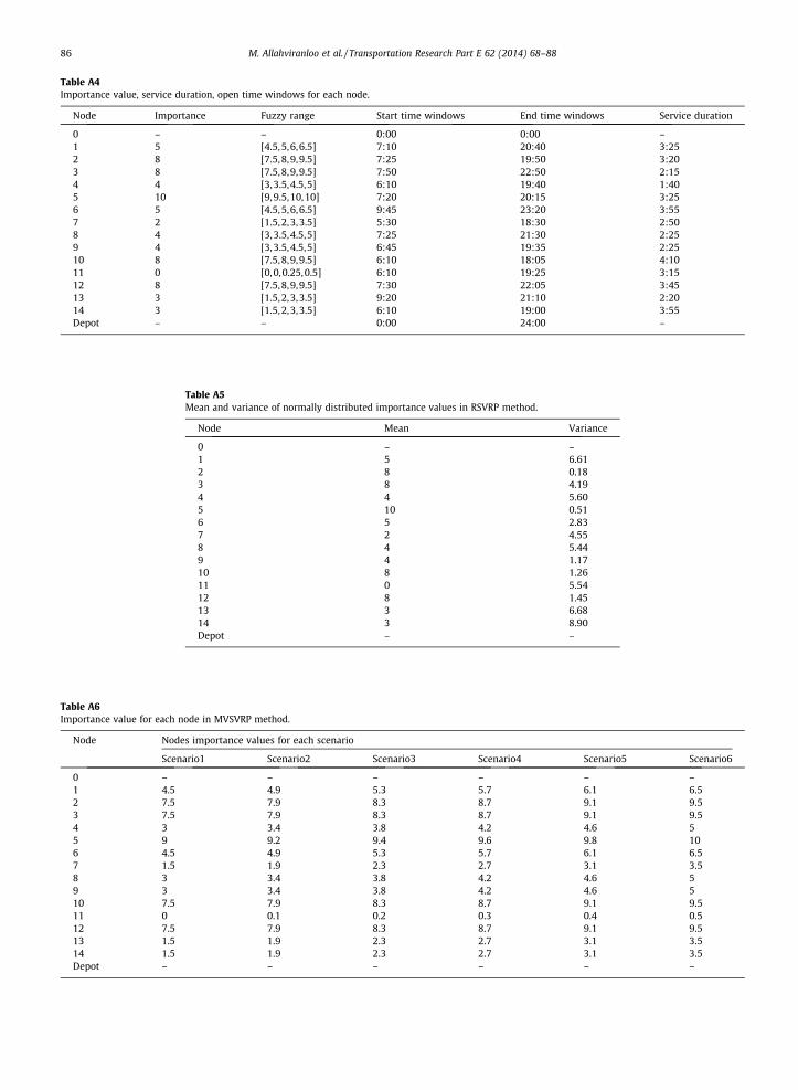
Table A4Importance value, service duration, open time windows for each node.

Node Importance Fuzzy range Start time windows End time windows Service duration

0 – – 0:00 0:00 –1 5 [4.5,5,6,6.5] 7:10 20:40 3:252 8 [7.5,8,9,9.5] 7:25 19:50 3:203 8 [7.5,8,9,9.5] 7:50 22:50 2:154 4 [3,3.5,4.5,5] 6:10 19:40 1:405 10 [9,9.5,10,10] 7:20 20:15 3:256 5 [4.5,5,6,6.5] 9:45 23:20 3:557 2 [1.5,2,3,3.5] 5:30 18:30 2:508 4 [3,3.5,4.5,5] 7:25 21:30 2:259 4 [3,3.5,4.5,5] 6:45 19:35 2:2510 8 [7.5,8,9,9.5] 6:10 18:05 4:1011 0 [0, 0,0.25,0.5] 6:10 19:25 3:1512 8 [7.5,8,9,9.5] 7:30 22:05 3:4513 3 [1.5,2,3,3.5] 9:20 21:10 2:2014 3 [1.5,2,3,3.5] 6:10 19:00 3:55Depot – – 0:00 24:00 –

Table A5Mean and variance of normally distributed importance values in RSVRP method.

Node Mean Variance

0 – –1 5 6.612 8 0.183 8 4.194 4 5.605 10 0.516 5 2.837 2 4.558 4 5.449 4 1.1710 8 1.2611 0 5.5412 8 1.4513 3 6.6814 3 8.90Depot – –

Table A6Importance value for each node in MVSVRP method.

Node Nodes importance values for each scenario

Scenario1 Scenario2 Scenario3 Scenario4 Scenario5 Scenario6

0 – – – – – –1 4.5 4.9 5.3 5.7 6.1 6.52 7.5 7.9 8.3 8.7 9.1 9.53 7.5 7.9 8.3 8.7 9.1 9.54 3 3.4 3.8 4.2 4.6 55 9 9.2 9.4 9.6 9.8 106 4.5 4.9 5.3 5.7 6.1 6.57 1.5 1.9 2.3 2.7 3.1 3.58 3 3.4 3.8 4.2 4.6 59 3 3.4 3.8 4.2 4.6 510 7.5 7.9 8.3 8.7 9.1 9.511 0 0.1 0.2 0.3 0.4 0.512 7.5 7.9 8.3 8.7 9.1 9.513 1.5 1.9 2.3 2.7 3.1 3.514 1.5 1.9 2.3 2.7 3.1 3.5Depot – – – – – –



7. Conclusion

In this paper we take a step back from the current trend of applying a recourse assumption to probabilistic routing prob-lems, even those that should not allow recourse. We show with a simple illustration that a selective problem under uncer-tainty with no recourse can offer more value than a conventional TSP. Three optimization objectives are proposed under thisproblem variation: maximizing minimum reliability, maximizing robustness, and maximizing the importance of the solutionwhen the importance of each node is fuzzy.

In relation to the literature, the contributions of this work are: (1) the argument that certain stochastic applications ofvehicle routing should not allow recourse, and in those cases the VRP solution is inferior to the more generalized SVRP;(2) developing three new SVRP formulations under uncertainty to address the lack of stochastic extensions of SVRP untilnow; (3) proposing three sets of parallel genetic algorithms to find solutions for large network application of SVRP or forSVRP with nonlinear terms; and (4) demonstration of the applicability of the proposed method to humanitarian logistics.

These selective routing models offer significant potential for disaster management, particularly the FSVRP because of thenaturally fuzzy nature of many elements in a disaster relief operation. Using the a-cut method, FSVRP provides a spectrum ofoptimal solutions based on the degree of uncertainty. Although there is uncertainty associated with the importance of eachnode, we demonstrate that there may exist a subset of nodes which can be informative to decision-makers if it is not empty.In the case of humanitarian logistics, this insight has a direct application in the local social network integration argued for inthe literature.

Despite the generally larger number of applications in uncertain problems with recourse, there are also many opportu-nities for future studies in problems without recourse. The formulations presented in this work open the way for alternativemodels (e.g. convex robust optimization). The results for the small network can be replicated and more efficient algorithmscan be designed specifically for this type of problem. Of immediate interest is the application of FSVRP to an actual disasterregion. We speculate that the combination of different social networks, the type of disaster, and resources available will lendto different distribution topologies. Although the present study precludes recourse, it would be interesting to comparedynamic routing strategies based on selective VRP solutions with conventional VRP solutions.

Appendix A

Table A1 shows the results of solving different instances using GA, PGA_1, PGA_2, and PGA_3 for FSVRP formulation. Inthese instances number of nodes are generated from a uniform distribution in the range of [8,16]. Other parameters such astravel time and cost in network, activity duration, start time and end time windows are generated randomly as explained inTable A2.

See Figs. A1 and A2 and Tables A1–A6.

References

Agra, A., Christiansen, M., Figueiredo, R., Hvattum, L.M., Poss, M., Requejo, C., 2013. The robust vehicle routing problem with time windows. Computers & OR40 (3), 856–866.

Allahviranloo, M., Recker, W.W., 2013. Modeling uncertainty in households’ activity engagement decisions. In: The Proceedings of 92nd Annual Meeting ofTransportation Research Board of the National Academies, Washington, DC, pp. 13–2876.

Ben-Tal, A., Nemirovski, A., 1998. Robust convex optimization. Mathematics of Operations Research 23 (4), 769–805.Berger, J., Barkaoui, M., 2004. A parallel hybrid genetic algorithm for the vehicle routing problem with time windows. Computers and Operations Research

31 (12), 2037–2053.Bertsimas, D.J., 1988. Probabilistic Combinatorial Optimization Problems. PhD Dissertation, Massachusetts Institute of Technology, Cambridge, MA.Bertsimas, D.J., Jaillet, P., Odoni, A.R., 1990. A priori optimization. Operations Research 38 (6), 1019–1033.Bertsimas, D.J., 1992. A vehicle routing problem with stochastic demand. Operations Research 40 (3), 574–585.Bianchi, L., Birattari, M., Chiarandini, M., Manfrin, M., Mastrolilli, M., Paquete, L., Rossi-Doria, O., Schiavinotto, T., 2006. Hybrid metaheuristics for the vehicle

routing problem with stochastic demands. Journal of Mathematical Modelling and Algorithms 5 (1), 91–110.Bozorgi-Amiri, A., Jabalameli, M.S., Mirzapour Al-e-Hashem, S.M.J., 2013. A multi-objective robust stochastic programming model for disaster relief logistics

under uncertainty. OR Spectrum 35 (4), 905–933.Cantú-Paz, E., 1998. A survey of parallel genetic algorithms. Calculateurs Parallèles, Réseaux et Systèmes Répartis 10 (2), 141–171.Cao, E., Lai, M., 2010. The open vehicle routing problem with fuzzy demands. Expert Systems with Applications 37 (3), 2405–2411.Chen, A., Subprasom, K., Ji, Z., 2006. A simulation-based multi-objective genetic algorithm (SMOGA) procedure for BOT network design problem.

Optimization Engineering 7 (3), 225–247.Chen, A., Kim, J., Zhou, Z., Chootinan, P., 2007. Alpha reliable network design problem. Transportation Research Record: Journal of the Transportation

Research Board 2029, 49–57.Chen, L., Miller-Hooks, E., 2012. Optimal team deployment in urban search and rescue. Transportation Research Part B 46 (8), 984–999.Chow, J.Y.J., Regan, A.C., 2011a. Network-based real option models. Transportation Research Part B 45 (4), 682–695.Chow, J.Y.J., Regan, A.C., 2011b. Real option pricing of network design investments. Transportation Science 45 (1), 50–63.Chow, J.Y.J., Liu, H., 2012. Generalized profitable tour problems for online activity routing systems. Transportation Research Record: Journal of the

Transportation Research Board 2284, 1–9.Chow, J.Y.J., 2013. Activity-based travel scenario analysis with routing problem reoptimization. Computer-Aided Civil and Infrastructure Engineering, in

press, doi: 10.1111/mice.12023.Chow, J.Y.J., Regan, A.C., 2013. A surrogate-based multiobjective metaheuristic and network degradation simulation model for robust toll pricing.

Optimization and Engineering. http://dx.doi.org/10.1007/s11081-013-9227-5.Daskin, M.S., Hesse, M., 1997. a-Reliable p-minimax regret: a new model for strategic facility location modeling. Location Science 5 (4), 227–246.Feillet, D., Dejax, P., Gendreau, M., 2005. Traveling salesman problems with profits. Transportation Science 39 (2), 188–205.FEMA/USACE, 2008. IS-26 Guide to Points of Distribution.

http://refhub.elsevier.com/S1366-5545(13)00198-1/h0021






















http://dx.doi.org/10.1007/s11081-013-9227-5




Gan, L.P., Recker, W., 2013. Stochastic preplanned household activity pattern problem with uncertain activity participation (SHAPP). Transportation Science47 (3), 439–454.

Gendreau, M., Laporte, G., Séguin, R., 1995. An exact algorithm for the vehicle routing problem with stochastic demands and customers. TransportationScience 29 (2), 143–155.

Gendreau, M., Laporte, G., Séguin, R., 1996a. Stochastic vehicle routing. European Journal of Operational Research 88 (1), 3–12.Gendreau, M., Laporte, G., Séguin, R., 1996b. A tabu search heuristic for the vehicle routing problem with stochastic demands and customers. Operations

Research 44 (3), 469–477.Ghiani, G., Guerriero, F., Laporte, G., Musmanno, R., 2003. Real-time vehicle routing: solution concepts, algorithms and parallel computing strategies.

European Journal of Operational Research 151 (1), 1–11.Gribkovskaia, I., Laporte, G., Shyshou, A., 2008. The single vehicle routing problem with deliveries and selective pickups. Computers and Operations

Research 35 (9), 2908–2924.Gupta, R., Singh, B., Pandey, D., 2010. Fuzzy vehicle routing problem with uncertainty in service time. International Journal of Contemporary Mathematical

Sciences 5 (11), 497–507.He, Y., Xu, J., 2005. A class of random fuzzy programming model and its application to vehicle routing problem. World Journal of Modelling and Simulation 1

(1), 3–11.Ho, W., Hob, G.T.S., Jib, P., Lau, H.C.W., 2008. A hybrid genetic algorithm for the multi-depot vehicle routing problem. Engineering Applications of Artificial

Intelligence 21, 548–557.Holguín-Veras, J., Jaller, M., Wachtendorf, T., 2012. Comparative performance of alternative humanitarian logistic structures after the Port-au-Prince

earthquake: ACEs, PIEs, and CANs. Transportation Research Part A 46 (10), 1623–1640.Huang, M., Smilowitz, K., Balcik, B., 2012. Models for relief routing: equity, efficiency and efficacy. Transportation Research Part E 48 (1), 2–18.Jaillet, P., 1988. A priori solution of a traveling salesman problem in which a random subset of the customers are visited. Operations Research 36 (6), 929–

936.Ji, Z., Kim, Y.S., Chen, A., 2011. Multi-objective a-reliable path finding in stochastic networks with correlated link costs: a simulation-based multi-objective

genetic algorithm approach (SMOGA). Expert Systems with Applications 38 (3), 1515–1528.Kenyon, A.S., Morton, D.P., 2003. Stochastic vehicle routing with random travel times. Transportation Science 37 (1), 69–82.Kuo, R.J., Chiu, C.Y., Lin, Y.J., 2004. Integration of fuzzy theory and ant algorithm for vehicle routing problem with time window. In: IEEE Annual Meeting of

the Fuzzy Information 2.Lam, T.C., Small, K.A., 2001. The value of time and reliability: measurement from a value pricing experiment. Transportation Research Part E 37 (2–3), 231–

251.Laporte, G., Martello, S., 1990. The selective traveling salesman problem. Discrete Applied Mathematics 26, 193–207.Laporte, G., Louveaux, F.V., van Hamme, L., 2002. An integer L-shaped algorithm for the capacitated vehicle routing problem with stochastic demands.

Operations Research 50 (3), 415–423.Li, Z.C., Lam, W.H.K., Wong, S.C., Sumalee, A., 2012. Environmentally sustainable toll design for congested road networks with uncertain demand.

International Journal of Sustainable Transportation 6 (3), 127–155.Liu, B., 2009. Theory and Practice of Uncertain Programming, UTLAB, third ed.Moghaddam, B.F., Ruiz, R., Sadjadi, S.J., 2012. Vehicle routing problem with uncertain demands: an advanced particle swarm algorithm. Computers and

Industrial Engineering 62 (1), 306–317.Mulvey, J.M., Vanderbei, R.J., Zenio, S.A., 1995. Robust optimization of large-scale systems. Operations Research 43 (2), 264–281.Ng, M., Waller, S.T., 2009. Reliable system-optimal network design. Transportation Research Record: Journal of the Transportation Research Board 2090, 68–

74.Ochi, L.S., Vianna, D.S., Drummond, L.M.A., Victor, O.V., 1998. A parallel evolutionary algorithm for the vehicle routing problem with heterogeneous fleet.

Future Generation Computer Systems 14 (5-6), 285–292.Powell, W.B., Simao, H.P., Bouzaiene-Ayari, B., 2012. Approximate dynamic programming in transportation and logistics: a unified framework. EURO Journal

of Transportation and Logistics 1 (3), 237–284.Recker, W.W., 1995. The household activity pattern problem: general formulation and solution. Transportation Research Part B 29 (1), 61–77.Regan, A.C., Mahmassani, H.S., Jaillet, P., 1996. Dynamic decision making for commercial fleet operations using real time information. Transportation

Research Record: Journal of the Transportation Research Board 1537, 91–97.Shapiro, A.F., 2009. Fuzzy random variables. Insurance: Mathematics and Economics 44 (2), 307–314.Sheu, J.B., 2007. An emergency logistics distribution approach for quick response to urgent relief demand in disasters. Transportation Research Part E 43 (6),

687–709.Sheu, J.B., 2010. Dynamic relief-demand management for emergency logistics operations under large-scale disasters. Transportation Research Part E 46 (1),

1–17.Stewart, W.R., Golden, B.L., 1983. Stochastic vehicle routing: a comprehensive approach. European Journal of Operational Research 14 (4), 371–385.Sungur, I., Ordóñez, F., Dessouky, M., 2008. A robust optimization approach for the capacitated vehicle routing problem with demand uncertainty. IIE

Transactions 40 (5), 509–523.Tan, K.C., Cheong, C.Y., Goh, C.K., 2007. Solving multiobjective vehicle routing problem with stochastic demand via evolutionary computation. Discrete

Optimization 177 (2), 813–839.Tang, J., Pan, Z., Fung, R.Y.K., Lau, H., 2009. Vehicle routing problem with fuzzy time windows. Fuzzy Sets and Systems 160 (5), 683–695.Tasgetiren, M.F., Smith, A.E., 2000. A genetic algorithm for the orienteering problem. In: Proceedings of the Congress on Evolutionary Computation 2, IEEE,

pp. 910–915.Teodorovic, D., Pavkovic, G., 1996. The fuzzy set theory approach to the vehicle routing problem when demand at nodes is uncertain. Fuzzy Sets and

Systems 82 (3), 307–317.Teodorovic, D., Radivojevic, G., 2000. A fuzzy logic approach to dynamic Dial-A-Ride problem. Fuzzy Sets and Systems 116 (1), 23–33.Tong, S., 1994. Interval number and fuzzy number linear programmings. Fuzzy Sets and Systems 66 (3), 301–306.Valle, C.A., Salles da Cunha, A., Mateus, G.R., Martinez, L.C., 2009. Exact algorithms for a selective Vehicle Routing Problem where the longest route is

minimized. Electronic Notes in Discrete Mathematics 35, 133–138.Van Hentenryck, P., Bent, R., Coffrin, C., 2010. Strategic planning for disaster recovery with stochastic last mile distribution. Integration of AI and OR

Techniques in Constraint Programming for Combinatorial Optimization Problems, LNCS 6140, pp. 318–333.Wang, H.F., Wen, Y.P., 2002. Time-constrained Chinese postman problems. Computers & Mathematics with Applications 44 (3–4), 375–387.Wardman, M., 1998. The value of travel time: a review of British evidence. Journal of Transport Economics and Policy 32 (3), 285–316.Xu, J., Yan, F., Li, S., 2011. Vehicle routing optimization with soft time windows in a fuzzy random environment. Transportation Research Part E 47 (6), 1075–

1091.Yin, Y., 2008. Robust optimal traffic signal timing. Transportation Research Part B 42 (10), 911–924.Zheng, Y., Liu, B., 2006. Fuzzy vehicle routing model with credibility measure and its hybrid intelligent algorithm. Applied Mathematics and Computation

176 (2), 673–683.Zimmermann, H.J., 1978. Fuzzy programming and linear programming with several objective functions. Fuzzy Sets and Systems 1 (1), 45–56.Zimmermann, Hans-Jurgen, 1996. Fuzzy Set Theory and Its Applications. Kluwer Academic, Massachusetts.







































































transportation research part e - its news | institute … · selective vehicle routing ... network...

Documents