Transition on a Variable Bluntness 7-Degree Cone at

High Reynolds Number

Joseph S. Jewell*

U.S. Air Force Research Laboratory, Wright-Patterson AFB, OH 45433, USA

Richard E. Kennedy� and Stuart J. Laurence�

University of Maryland, College Park, MD 20742, USA

Roger L. Kimmel§

U.S. Air Force Research Laboratory, Wright-Patterson AFB, OH 45433, USA

The effects of bluntness and swallowing length on transition on an 7-degree cone at zeroangle of attack in Mach 6 high Reynolds number flow are studied experimentally and an-alyzed with the STABL computational fluid dynamics code package. Mean flow solutionsand PSE-Chem stability analyses for a total of 7 different nose tip bluntnesses, ranging fromsharp to 15.24 mm radius, are obtained. For the sharpest cases, NTr ≈ 7, but as bluntnessincreases and the calculated swallowing distance lengthens, the computed N-factor at theexperimentally-observed transition location drops below the level at which Mack’s secondmode would be expected to lead to transition. These results indicate that the dominantinstability mechanism for the bluntest cases is not the second mode. The results are consis-tent with an earlier seminal work in the same facility performed by Stetson on an 8-degreevariable-bluntness cone, and are the first to directly measure second mode instabilities inthis facility. High-speed schlieren visualizations were were used to measure disturbancepropagation speeds and frequency spectra for second mode wavepackets, in the thinnestboundary layers (0.50 mm and smaller), and at the highest frequencies (∼1 MHz), at whichthis technique has been applied to date. The observed peak disturbance frequencies agreewell with the predicted peak N-factor disturbance frequencies from stability analysis. Thisdemonstrates that high-speed schlieren with appropriate analysis is a useful tool for mea-suring instabilities in a frequency regime that is challenging for pressure transducers.

I. Introduction

Boundary layer transition is a critical factor in the design of hypersonic vehicles, with profound impacton both heat transfer and control characteristics. While many practical aerospace vehicles are blunt, themechanisms that lead to boundary layer instability and transition on sharp bodies are more thoroughlyunderstood at present. Over the past half century, a wealth of relevant wind tunnel and flight data has beenacquired. Analytical and computational techniques, as well as the rapid development of economical andpowerful computer processors, have made possible comprehensive computational analysis of experimentaldata sets as they are acquired. Furthermore, modern high-speed schlieren imaging techniques have enabledthe direct measurement of second mode instabilities for the first time in this facility. This work aids inunderstanding past transition experiments undertaken at high Reynolds number and demonstrates thathigh-speed schlieren is a useful tool for measuring instabilities in frequency regimes where standard pressure

*Research Scientist (Spectral Energies, LLC), AFRL/RQHF. AIAA Senior Member. jjewell@alumni.caltech.edu�Graduate Student, Department of Aerospace Engineering. AIAA Student Member.�Assistant Professor, Department of Aerospace Engineering. AIAA Senior Member.§Principal Aerospace Engineer, AFRL/RQHF. AIAA Associate Fellow.

1 of 14

American Institute of Aeronautics and AstronauticsCleared for Public Release, Case Number: 88ABW-2017-6156.

2018 AIAA Aerospace Sciences Meeting

8–12 January 2018, Kissimmee, Florida

10.2514/6.2018-1822

Copyright © 2018 by the American Institute of Aeronautics and Astronautics, Inc.

All rights reserved.

AIAA SciTech Forum

transducers may not perform well (∼1 MHz).

Between 1978 and 1982, K. F. Stetson performed a total of 196 sharp- and blunt-cone experiments1 on athin-walled 8-degree half-angle, 4 in.-base cone in the Air Force Research Laboratory (AFRL) Mach 6 HighReynolds Number facility. These experiments were reported in a 1983 paper2 along with results from AEDCTunnel F with a larger cone at Mach 9. The AFRL Mach 6 results recently received computational analysis3

indicating that the Mack second mode was unlikely to be the dominant instability mechanism for nose tipswith radius larger than 1 mm. In the present work, a total of 132 sharp- and blunt-cone experiments wereperformed on a smooth, thick-walled 7-degree half-angle, 4 in.-base cone at 0 AoA in the same facility, andsimilar computational analysis indicates that the dominant instability mechanism for the bluntest cases is,again, not the second mode.

The AFRL Mach 6 facility operates at stagnation pressure p0 from 700 to 2100 psi. Details of these conditions,along with an intermediate case, are presented in Table 1. A total of 65 experiments1 at unique conditionscomprise the present Mach 6 results (see Section III). Mean-flow and stability calculations for each conditionwere performed at a computational cost of about 100 processor-hours each.

Table 1. Summary of sample inflow conditions computed for each bluntness value, with one intermediate value pre-sented. These conditions encompass the operating envelope of the AFRL Mach 6 High Reynolds Number facility.

p0 unit Re∞ M∞ ρ∞ P∞ T∞ U∞ Tw/T0

[psi] [MPa] ×106/m - [kg/m3] [kPa] [K] [m/s] -

700 4.83 30.7 5.9 0.154 3.40 76.7 1038 0.56

1400 9.65 61.4 5.9 0.308 6.80 76.7 1038 0.56

2100 14.5 92.1 5.9 0.461 10.2 76.7 1038 0.56

II. Computational Methods

0 0.05 0.1 0.15 0.2 0.25 0.3 0.35 0.4 0.450

0.05

0.1

[m]

[m]

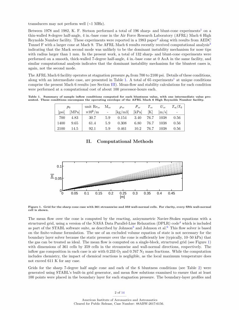
Figure 1. Grid for the sharp cone case with 361 streamwise and 359 wall-normal cells. For clarity, every fifth wall-normalcell is shown.

The mean flow over the cone is computed by the reacting, axisymmetric Navier-Stokes equations with astructured grid, using a version of the NASA Data Parallel-Line Relaxation (DPLR) code4 which is includedas part of the STABL software suite, as described by Johnson5 and Johnson et al.6 This flow solver is basedon the finite-volume formulation. The use of an excluded volume equation of state is not necessary for theboundary layer solver because the static pressure over the cone is sufficiently low (typically, 10–50 kPa) thatthe gas can be treated as ideal. The mean flow is computed on a single-block, structured grid (see Figure 1)with dimensions of 361 cells by 359 cells in the streamwise and wall-normal directions, respectively. Theinflow gas composition in each case is air with 0.233 O2 and 0.767 N2 mass fractions. While the computationincludes chemistry, the impact of chemical reactions is negligible, as the local maximum temperature doesnot exceed 611 K for any case.

Grids for the sharp 7-degree half angle cone and each of the 6 bluntness conditions (see Table 2) weregenerated using STABL’s built-in grid generator, and mean flow solutions examined to ensure that at least100 points were placed in the boundary layer for each stagnation pressure. The boundary-layer profiles and

2 of 14

American Institute of Aeronautics and AstronauticsCleared for Public Release, Case Number: 88ABW-2017-6156.

edge properties are extracted from the mean flow solutions during post-processing. The wall-normal span ofthe grid increases down the length of the cone, from 0.25 mm at the tip to 50 mm at the base, allowing forthe shock to be fully contained within the grid for all cases tested. The grid is clustered at the wall as well asat the nose in order to capture the gradients in these locations. The ∆y+ value for the grid, extracted fromthe DPLR solution for each case, is everywhere less than 1, where ∆y+ is a measure of local grid quality atthe wall in the wall-normal direction.

Table 2. Summary of grids generated for the present study, each corresponding to a different sharp or blunt nose tipused in the present study. For simplicity and to match the Stetson2 nomenclature, bluntness as a percentage of thebase radius of 2.0 inches is used to label the cases analyzed in the present work.

RN Bluntness

in. mm %

0 0 0

0.02 0.508 1

0.06 1.524 3

0.10 2.540 5

0.20 5.080 10

0.40 10.16 20

0.60 15.24 30

III. Mean Flow-Based Transition Correlations

Following Stetson2 and Jewell and Kimmel3 results are reported by normalizing the transition Reynoldsnumbers for blunted cones by the transition Reynolds numbers for sharp cones at the same inflow conditions,which are calculated as:

XTrB

XTrS

=(ReXe )TrB

(ReXe )TrS

(Reunit)eS

(Reunit)eB

Here, subscript “S” indicates values for a sharp tip, “B” values for a given blunt tip at the same condition,and “e” conditions at the boundary layer edge. The boundary layer edge, throughout the present work, isdefined as the point at which the derivative of the enthalpy along a line extending orthogonally from thesurface of the cone approaches zero.

The entropy layer swallowing length estimate of Rotta7 (XSW), as applied by Stetson and Rushton,8 is alsoused to correlate the results. The entropy layer is depicted directly by using the DPLR solution for eachcase (gas composition, temperature, and pressure) as the input for an entropy calculation at each cell, whichis performed using the Cantera9 thermodynamics software.

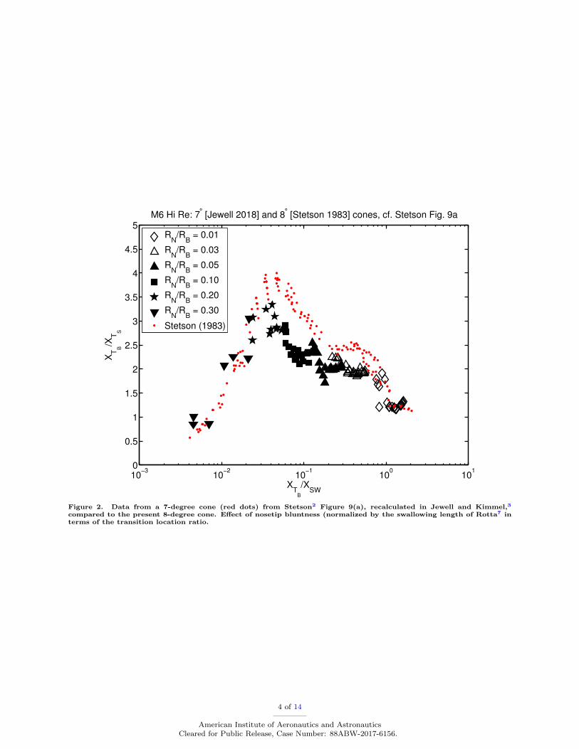
Figure 9 in Stetson2 summarizes his results, and was recreated using the transition locations reported inStetson1 and new condition computations in Figures 5 and 6 of Jewell and Kimmel.3 The present 7-degreeresults are compared to the historical data below as Figures 2 and 3.

IV. Stability Computations

The stability analyses are performed using the PSE-Chem solver, which is also part of the STABL softwaresuite. PSE-Chem10 solves the reacting, two-dimensional, axisymmetric, linear parabolized stability equations(PSE) to predict the amplification of disturbances as they interact with the boundary layer. The PSE-Chemsolver includes finite-rate chemistry and translational-vibrational energy exchange. The parabolized stabilityequations predict the amplification of disturbances as they interact with the boundary layer.

The band of amplified frequencies within the boundary layer predicted by Linear Stability Theory (LST) ispresented in a contour plot in terms of amplification −αi in Figure 4 for three cases equivalent to experimentsin the present data set. The most amplified frequency predicted by a simple model based on edge velocity

3 of 14

American Institute of Aeronautics and AstronauticsCleared for Public Release, Case Number: 88ABW-2017-6156.

10−3

10−2

10−1

100

101

0

0.5

1

1.5

2

2.5

3

3.5

4

4.5

5

XT

B

/XSW

XT

B

/XT

S

M6 Hi Re: 7° [Jewell 2018] and 8

° [Stetson 1983] cones, cf. Stetson Fig. 9a

RN/R

B = 0.01

RN/R

B = 0.03

RN/R

B = 0.05

RN/R

B = 0.10

RN/R

B = 0.20

RN/R

B = 0.30

Stetson (1983)

Figure 2. Data from a 7-degree cone (red dots) from Stetson2 Figure 9(a), recalculated in Jewell and Kimmel,3

compared to the present 8-degree cone. Effect of nosetip bluntness (normalized by the swallowing length of Rotta7 interms of the transition location ratio.

4 of 14

American Institute of Aeronautics and AstronauticsCleared for Public Release, Case Number: 88ABW-2017-6156.

10−3

10−2

10−1

100

101

0

0.2

0.4

0.6

0.8

1

1.2

1.4

1.6

1.8

XT

B

/XSW

(Re

XT

) B/(

Re

XT

) S

M6 Hi Re: 7° [Jewell 2018] and 8

° [Stetson 1983] cones, cf. Stetson Fig. 9b

RN/R

B = 0.01

RN/R

B = 0.03

RN/R

B = 0.05

RN/R

B = 0.10

RN/R

B = 0.20

RN/R

B = 0.30

Stetson (1983)

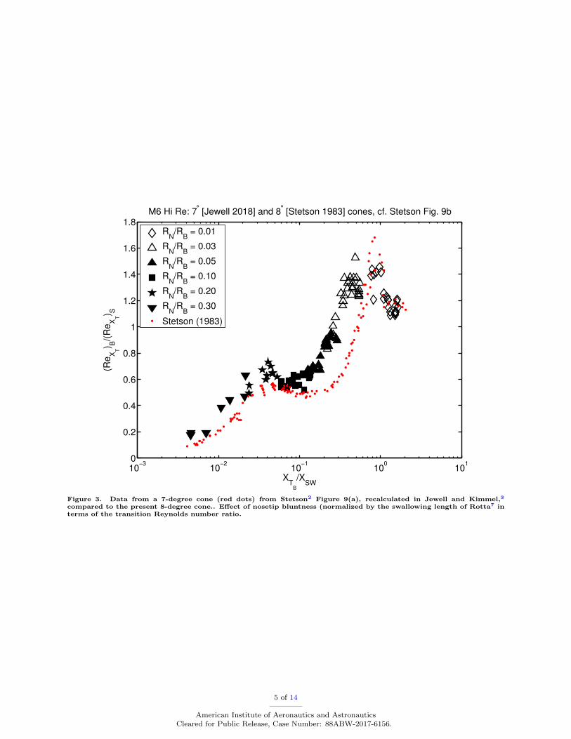
Figure 3. Data from a 7-degree cone (red dots) from Stetson2 Figure 9(a), recalculated in Jewell and Kimmel,3

compared to the present 8-degree cone.. Effect of nosetip bluntness (normalized by the swallowing length of Rotta7 interms of the transition Reynolds number ratio.

5 of 14

American Institute of Aeronautics and AstronauticsCleared for Public Release, Case Number: 88ABW-2017-6156.

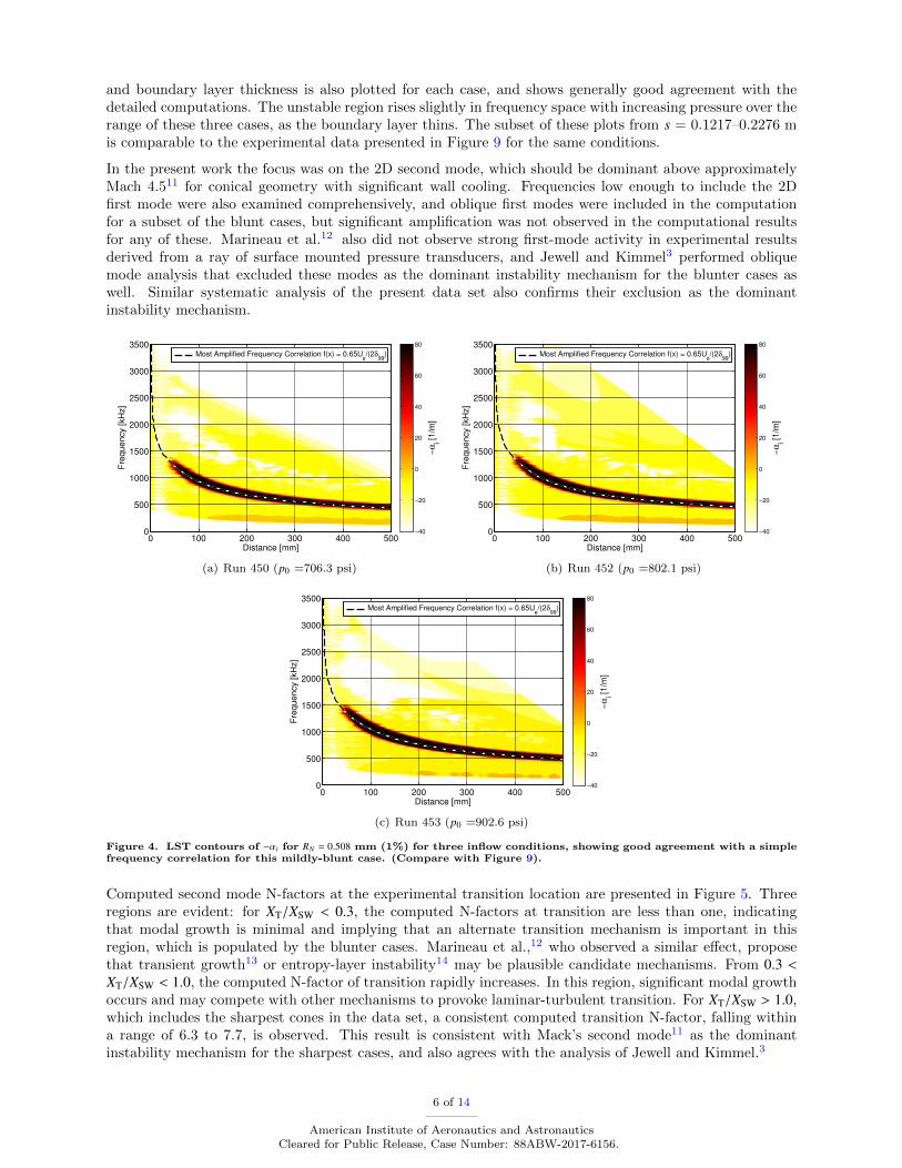
and boundary layer thickness is also plotted for each case, and shows generally good agreement with thedetailed computations. The unstable region rises slightly in frequency space with increasing pressure over therange of these three cases, as the boundary layer thins. The subset of these plots from s = 0.1217–0.2276 mis comparable to the experimental data presented in Figure 9 for the same conditions.

In the present work the focus was on the 2D second mode, which should be dominant above approximatelyMach 4.511 for conical geometry with significant wall cooling. Frequencies low enough to include the 2Dfirst mode were also examined comprehensively, and oblique first modes were included in the computationfor a subset of the blunt cases, but significant amplification was not observed in the computational resultsfor any of these. Marineau et al.12 also did not observe strong first-mode activity in experimental resultsderived from a ray of surface mounted pressure transducers, and Jewell and Kimmel3 performed obliquemode analysis that excluded these modes as the dominant instability mechanism for the blunter cases aswell. Similar systematic analysis of the present data set also confirms their exclusion as the dominantinstability mechanism.

Distance [mm]

Fre

quency [kH

z]

0 100 200 300 400 5000

500

1000

1500

2000

2500

3000

3500Most Amplified Frequency Correlation f(x) = 0.65U

e/(2δ

99)

−α

i [1/m

]

−40

−20

0

20

40

60

80

(a) Run 450 (p0 =706.3 psi)

Distance [mm]

Fre

quency [kH

z]

0 100 200 300 400 5000

500

1000

1500

2000

2500

3000

3500Most Amplified Frequency Correlation f(x) = 0.65U

e/(2δ

99)

−α

i [1/m

]

−40

−20

0

20

40

60

80

(b) Run 452 (p0 =802.1 psi)

Distance [mm]

Fre

quency [kH

z]

0 100 200 300 400 5000

500

1000

1500

2000

2500

3000

3500Most Amplified Frequency Correlation f(x) = 0.65U

e/(2δ

99)

−α

i [1/m

]

−40

−20

0

20

40

60

80

(c) Run 453 (p0 =902.6 psi)

Figure 4. LST contours of −αi for RN = 0.508 mm (1%) for three inflow conditions, showing good agreement with a simplefrequency correlation for this mildly-blunt case. (Compare with Figure 9).

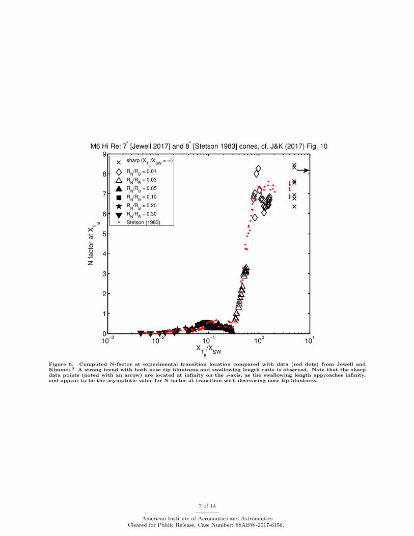
Computed second mode N-factors at the experimental transition location are presented in Figure 5. Threeregions are evident: for XT/XSW < 0.3, the computed N-factors at transition are less than one, indicatingthat modal growth is minimal and implying that an alternate transition mechanism is important in thisregion, which is populated by the blunter cases. Marineau et al.,12 who observed a similar effect, proposethat transient growth13 or entropy-layer instability14 may be plausible candidate mechanisms. From 0.3 <XT/XSW < 1.0, the computed N-factor of transition rapidly increases. In this region, significant modal growthoccurs and may compete with other mechanisms to provoke laminar-turbulent transition. For XT/XSW > 1.0,which includes the sharpest cones in the data set, a consistent computed transition N-factor, falling withina range of 6.3 to 7.7, is observed. This result is consistent with Mack’s second mode11 as the dominantinstability mechanism for the sharpest cases, and also agrees with the analysis of Jewell and Kimmel.3

6 of 14

American Institute of Aeronautics and AstronauticsCleared for Public Release, Case Number: 88ABW-2017-6156.

10−3

10−2

10−1

100

101

0

1

2

3

4

5

6

7

8

9

XT

B

/XSW

N f

acto

r a

t X

TB

M6 Hi Re: 7° [Jewell 2017] and 8

° [Stetson 1983] cones, cf. J&K (2017) Fig. 10

sharp (XT

B

/XSW

= ∞)

RN/R

B = 0.01

RN/R

B = 0.03

RN/R

B = 0.05

RN/R

B = 0.10

RN/R

B = 0.20

RN/R

B = 0.30

Stetson (1983)

Figure 5. Computed N-factor at experimental transition location compared with data (red dots) from Jewell andKimmel.3 A strong trend with both nose tip bluntness and swallowing length ratio is observed. Note that the sharpdata points (noted with an arrow) are located at infinity on the x-axis, as the swallowing length approaches infinity,and appear to be the asymptotic value for N-factor at transition with decreasing nose tip bluntness.

7 of 14

American Institute of Aeronautics and AstronauticsCleared for Public Release, Case Number: 88ABW-2017-6156.

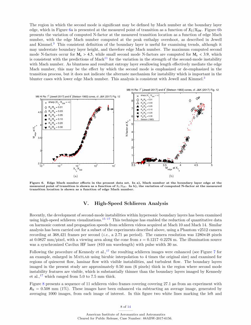
The region in which the second mode is significant may be defined by Mach number at the boundary layeredge, which in Figure 6a is presented at the measured point of transition as a function of XT/XSW. Figure 6bpresents the variation of computed N-factor at the measured transition location as a function of edge Machnumber, with the edge Mach number computed at the peak enthalpy overshoot, as described in Jewelland Kimmel.3 This consistent definition of the boundary layer is useful for examining trends, although itmay understate boundary layer height, and therefore edge Mach number. The maximum computed secondmode N-factors occur for Me > 4.5, while small second mode N-factors are computed for Me < 3.9, whichis consistent with the predictions of Mack11 for the variation in the strength of the second-mode instabilitywith Mach number. As bluntness and resultant entropy layer swallowing length effectively mediate the edgeMach number, this may be the effect by which the second mode is emphasized or de-emphasized in thetransition process, but it does not indicate the alternate mechanism for instability which is important in theblunter cases with lower edge Mach number. This analysis is consistent with Jewell and Kimmel.3

10−3

10−2

10−1

100

101

2.5

3

3.5

4

4.5

5

XT

B

/XSW

Me

dg

e a

t X

TB

M6 Hi Re: 7° [Jewell 2017] and 8

° [Stetson 1983] cones, cf. J&K (2017) Fig. 12

sharp (XT

B

/XSW

= ∞)

RN/R

B = 0.01

RN/R

B = 0.03

RN/R

B = 0.05

RN/R

B = 0.10

RN/R

B = 0.20

RN/R

B = 0.30

(a)

2.5 3 3.5 4 4.5 50

1

2

3

4

5

6

7

8

9

Medge

at XT

B

N f

acto

r a

t X

TB

M6 Hi Re: 7° [Jewell 2017] and 8

° [Stetson 1983] cones, cf. J&K (2017) Fig. 12

sharp (XT

B

/XSW

= ∞)

RN/R

B = 0.01

RN/R

B = 0.03

RN/R

B = 0.05

RN/R

B = 0.10

RN/R

B = 0.20

RN/R

B = 0.30

Stetson (1983)

(b)

Figure 6. Edge Mach number effects in the present data set. In a), Mach number at the boundary layer edge at themeasured point of transition is shown as a function of XT/XSW. In b), the variation of computed N-factor at the measuredtransition location is shown as a function of edge Mach number.

V. High-Speed Schlieren Analysis

Recently, the development of second-mode instabilities within hypersonic boundary layers has been examinedusing high-speed schlieren visualizations.15–17 This technique has enabled the reduction of quantitative dataon harmonic content and propagation speeds from schlieren videos acquired at Mach 10 and Mach 14. Similaranalysis has been carried out for a subset of the experiments described above, using a Phantom v2512 camerarecording at 368,421 frames per second (i.e., a 2.71 µs period). The camera resolution was 1280×48 pixelsat 0.0827 mm/pixel, with a viewing area along the cone from s = 0.1217–0.2276 m. The illumination sourcewas a synchronized Cavilux HF laser (810 nm wavelength) with pulse width 30 ns.

Following the procedure of Kennedy et al.,17 the resulting schlieren images were enhanced (see Figure 7 foran example, enlarged in Matlab using bicubic interpolation to 4 times the original size) and examined forregions of quiescent flow, laminar flow with visible instabilities, and turbulent flow. The boundary layersimaged in the present study are approximately 0.50 mm (6 pixels) thick in the region where second modeinstability features are visible, which is substantially thinner than the boundary layers imaged by Kennedyet al.,17 which ranged from 5.0 to 7.5 mm thick.

Figure 8 presents a sequence of 11 schlieren video frames covering covering 27.1 µs from an experiment withRN = 0.508 mm (1%). These images have been enhanced via subtracting an average image, generated byaveraging 1000 images, from each image of interest. In this figure two white lines marking the left and

8 of 14

American Institute of Aeronautics and AstronauticsCleared for Public Release, Case Number: 88ABW-2017-6156.

Figure 7. Run 450 (P0 = 706.3 psi) enhanced schlieren detail displaying (left to right) laminar flow with rope-likesecond mode instability features, an apparently quiescent region, and a turbulent region. The boundary layer in thisimage, and in Figure 8 is 6 pixels or ∼0.50 mm thick, and the viewing area is s = 0.1525–0.2024 m.

right edges of a wavepacket have been added to facilitate visual tracking. The white lines in the first imageindicate the extent of the identified wavepacket, and they are propagated downstream in subsequent imagesusing the average calculated wavepacket propagation speed.

Figure 8. Run 450 (P0 = 706.3 psi) enhanced schlieren sequence (full) covering 27.1 µs, with white lines indicatingthe extent of the identified wavepacket in the first image, shifted downstream in subsequent images using the averagecalculated wavepacket propagation speed. Each image is 10.59 cm long.

Wavepacket propagation speeds are calculated using a cross correlation between sequential images. Speedswere calculated from 5000 images (13.6 ms, or ∼12.2 m of flow length) in the middle of each run time.Wavepackets are identified through a Matlab implementation of the MUSIC (Multiple Signal Classification)algorithm.18 The number of wavepackets used for the calculation is different for each run, because more thanone strong wavepacket may be present in a single image. Typically, the standard deviations are 5–7% (95%confidence interval), which would improve with more pixels in the boundary layer, which would increasethe correlation coefficient through a higher-fidelity recording of the waves. Propagation speed calculationresults from four experiments are presented in Table 3. Turbulent convection velocities are not calculated,because the cross-correlation does not produce a peak. The calculated disturbance speeds are about 93% ofthe computed boundary layer edge velocity, which is close to previously reported second mode wavepacketpropagation speeds at higher Mach number,17 as well as leading-edge values for turbulent spot propagationspeeds at similar Mach numbers.19

Table 3. Mean wavepacket propagation speeds calculated by cross correlating 5000 sequential images (135.5 ms) fromeach experiment.

Run p0 T0 Uprop Uprop/Ue σ 2σ error No. of wavepackets

psi °R m/s m/s %

450 706.3 1009 890.8 0.922 26.5 5.96 5615

451 705.6 1008 893.8 0.929 26.3 5.88 5742

452 802.1 1007 896.6 0.932 33.3 7.42 7010

453 902.6 1008 892.2 0.927 27.0 6.06 7000

Spatial and frequency features of the wavepacket ensembles reported in Table 3 were analyzed. Pixel intensityversus time signals were reconstructed at the y/δ location of largest disturbance amplitude and interpolationwas used to remain at the fixed y/δ location as the boundary layer grew downstream. The signals were

9 of 14

American Institute of Aeronautics and AstronauticsCleared for Public Release, Case Number: 88ABW-2017-6156.

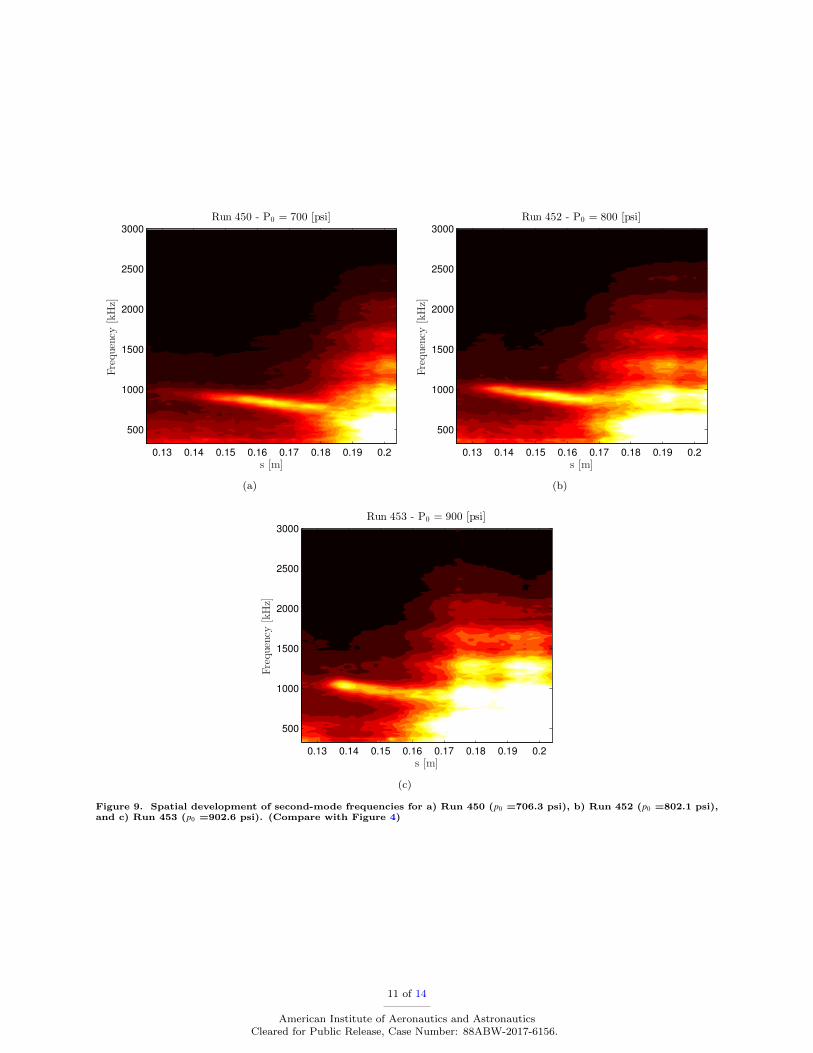
generated, as above, from 5000 images (13.6 ms) from each run. Spectra were computed using Welch’smethod averaging 200 windows with 50% overlap, with a Blackman windowing function applied. Resultsof this analysis for three conditions are presented in Figure 9. Note that the color scale is uncalibratedlogarithmic arbitrary units. As in Figure 4, the unstable region rises slightly in frequency space withincreasing pressure over the range of these three cases, as the boundary layer thins. The transition front,visible as a region of broadband disturbances downstream of the narrowband instability, also clearly movesforward with increasing pressure (this feature does not appear in the Figure 4 contours, as LST does notmodel turbulence).

Results become more noisy with higher p0, and the highest pressure at which data that were deemed suitablefor wavepacket analysis were acquired was the p0 = 902.6 psi case. While experiments were performedat higher pressures, the cross-correlation and frequency extraction for these cases were significantly morenoisy. This noise may be associated with insufficient pixel resolution in the boundary layer—the minimumnumber of pixels at p0 = 902.6 psi was about 4.5 in the upstream region, and there were even fewer in thethinner boundary layers at higher pressure. Furthermore, there are no clear harmonics present in the spectrapresented in Figures 9 and 10. This may also be a consequence of relatively low pixel counts in the extremelythin boundary layers. The banding at 400 kHz observed at higher Reynolds numbers may be an artifact,but is also possibly subharmonic resonance of the second mode.20

Figure 10(a) presents spectra observed from Run 450 (p0 =706.3 psi) at four different streamwise stationsfrom s = 0.141–0.165 m. As the boundary layer thickens with increasing downstream distance, the peakfrequency decreases and the magnitude of the peak (again, in arbitrary units) increases. The peak frequenciesfor this case at these four locations are compared with interpolated LST and PST peak instability frequencies,computed with STABL-2D in Section IV, in Figure 10(b). For LST, the reported frequencies are taken fromthe peak of the contour plot in Figure 4. For PSE, the reported frequencies are those associated with thelargest predicted N-factor at each s-location. Both LST and PSE curves exhibit the same general trendas the schlieren-derived peaks, but the PSE frequencies agree much more closely with the experimentallymeasured case. LST has a lower frequency as the peak growth occurs at a lower frequency than the peakamplitude.21

VI. Conclusions

A strong trend in transition N-factor for both nose tip bluntness and swallowing length ratio is observedin the results computed. As bluntness increases and the calculated swallowing distance lengthens, thecomputed N-factor at the experimentally-observed transition location drops below the level at which Mack’ssecond mode11 would be expected to lead to transition.22,23 These results indicate that the dominantinstability mechanism for the bluntest cases is likely not the second mode, which is consistent with recentblunt cone results12 at different conditions. Alternate instability mechanisms include transient growth,13

perhaps induced through particulate in the flow,24 and entropy-layer instability.14

Based upon the computed second-mode amplification factors eN, transition onset in the AFRL Mach 6High Reynolds Number facility is estimated to correspond to N ≈ 7 for the sharp and nearly sharp cases.These amplification values are high as compared to the more typical value of N ≈ 5–6 usually characterizinga “noisy” tunnel,25 but are consistent with previous results reported in the same facility by Jewell andKimmel.3

High-speed schlieren visualizations were acquired, and disturbance propagation speeds for second modewavepackets at several cases with RN = 0.508 mm (1%) were calculated by cross-correlating video frames.Spectra were also computed from the same images. These results represent the thinnest boundary layers(0.50 mm and smaller), and highest frequencies (∼1 MHz), at which this technique has been applied todate. The observed peak disturbance frequencies agree well with the predicted peak N-factor disturbancefrequencies as computed by PSE-Chem.

10 of 14

American Institute of Aeronautics and AstronauticsCleared for Public Release, Case Number: 88ABW-2017-6156.

s [m]

Frequency

[kHz]

Run 450 - P0 = 700 [psi]

0.13 0.14 0.15 0.16 0.17 0.18 0.19 0.2

500

1000

1500

2000

2500

3000

(a)

s [m]

Frequency

[kHz]

Run 452 - P0 = 800 [psi]

0.13 0.14 0.15 0.16 0.17 0.18 0.19 0.2

500

1000

1500

2000

2500

3000

(b)

s [m]

Frequency

[kHz]

Run 453 - P0 = 900 [psi]

0.13 0.14 0.15 0.16 0.17 0.18 0.19 0.2

500

1000

1500

2000

2500

3000

(c)

Figure 9. Spatial development of second-mode frequencies for a) Run 450 (p0 =706.3 psi), b) Run 452 (p0 =802.1 psi),and c) Run 453 (p0 =902.6 psi). (Compare with Figure 4)

11 of 14

American Institute of Aeronautics and AstronauticsCleared for Public Release, Case Number: 88ABW-2017-6156.

500 1000 1500 200010

−4

10−3

10−2

Frequency [kHz]

Pow

er[a.u.]

Run 450 - P0 = 700 [psi]

s = 0.141 [m]s = 0.149 [m]s = 0.157 [m]s = 0.165 [m]

(a) Power spectra from schlieren

0.145 0.15 0.155 0.16 0.165 0.17700

750

800

850

900

950

1000

s [m]

pe

ak f

req

ue

ncy [

kH

z]

Schlieren

LST

PSE

(b) Peak frequencies compared with computations

Figure 10. Power spectra (arbitrary units) for four different streamwise locations from Run 450 (p0 =706.3 psi), andobserved peak frequencies compared with LST and PST peak frequencies from Section IV.

12 of 14

American Institute of Aeronautics and AstronauticsCleared for Public Release, Case Number: 88ABW-2017-6156.

Acknowledgments

Joseph E. Wehrmeyer of AEDC generously arranged a loan of the Cavilux laser used in this work. Theauthors also thank Brian K.-Y. Lam, Jim Hayes, Servane Altman, and Benjamin Hagen for assistancerunning the Mach 6 Hi Re Facility. J. S. Jewell thanks Dr. Ross Wagnild of Sandia for his patient adviceon the use of the STABL code. A substantial portion of this research was performed while J. S. Jewell helda National Research Council Research Associateship Award at the Air Force Research Laboratory. R. E.Kennedy was supported by the National Defense Science and Engineering Graduate Fellowship.

References

1Stetson, K. F., “Notes related to previous AIAA papers on blunt cones,” Personal communication to S. P. Schneider, December2001, Purdue University.

2Stetson, K. F., “Nosetip Bluntness Effects on Cone Frustum Boundary Layer Transition in Hypersonic Flow,” Proceedings ofthe AlAA 16th Fluid and Plasma Dynamics Conference, AIAA-1983-1763, Danvers, Massachusetts, 1983.

3Jewell, J. S. and Kimmel, R. L., “Boundary Layer Stability Analysis for Stetsons Mach 6 Blunt Cone Experiments,” Journalof Spacecraft and Rockets, Vol. 54, No. 1, 2017, pp. 258–265.

4Wright, M. J., Candler, G. V., and Bose, D., “Data-parallel line relaxation method for the Navier-Stokes equations,” AIAAJournal , Vol. 36, No. 9, 1998, pp. 1603–1609.

5Johnson, H. B., Thermochemical Interactions in Hypersonic Boundary Layer Stability, Ph.D. thesis, University of Minnesota,Minneapolis, MN, 2000.

6Johnson, H. B., Seipp, T. G., and Candler, G. V., “Numerical study of hypersonic reacting boundary layer transition oncones,” Physics of Fluids, Vol. 10, 1998, pp. 2676–2685.

7Rotta, N. R., “Effects of nose bluntness on the boundary layer characteristics of conical bodies at hypersonic speeds,” NewYork University Report NYUAA-66-66, 1966.

8Stetson, K. F. and Rushton, G. H., “Shock Tunnel Investigation of Boundary-Layer Transition at M = 5.5,” AIAA Journal ,Vol. 5, No. 5, 1967, pp. 899–906.

9Goodwin, D., “Cantera: An object-oriented software toolkit for chemical kinetics, thermodynamics, and transport processes,”Available: http://code.google.com/p/cantera, 2009, Accessed: 12/12/2012.10Johnson, H. B. and Candler, G. V., “Hypersonic boundary layer stability analysis using PSE-Chem,” 35th Fluid DynamicsConference and Exhibit , AIAA, 2005, AIAA-2005-5023.11Mack, L. M., “Boundary-layer linear stability theory: Special course on stability and transition of laminar flow advisory groupfor aerospace research and development,” Tech. rep., 1984, AGARD Report No. 709, NATO, Neuilly sur Seine, France.12Marineau, E. C., Moraru, C. G., Lewis, D. R., Norris, J. D., Lafferty, J. F., Wagnild, R. M., and Smith, J. A., “Mach 10boundary-layer transition experiments on sharp and blunted cones,” 2014.13Reshotko, E., “Transient growth: A factor in bypass transition,” Physics of Fluids, Vol. 13, No. 5, 2001, pp. 1067–1075.14Kufner, E. and Dallmann, U., “Entropy-and Boundary Layer Instability of Hypersonic Cone Flows-Effects of Mean FlowVariations,” Laminar-Turbulent Transition, Springer, 1995, pp. 197–204.15Laurence, S. J., Wagner, A., and Hannemann, K., “Schlieren-based techniques for investigating instability development andtransition in a hypersonic boundary layer,” Experiments in Fluids, Vol. 55, No. 1782, 2014.16Laurence, S., Wagner, A., and Hannemann, K., “Experimental study of second-mode instability growth and breakdown in ahypersonic boundary layer using high-speed schlieren visualization,” Journal of Fluid Mechanics, Vol. 797, 2016, pp. 471–503.17Kennedy, R. E., Laurence, S. J., Smith, M. S., and Marineau, E. C., “Feedback Stabilized Laser Differential Interferometryfor Supersonic Blunt Body Receptivity Experiments,” AIAA SciTech 2017 , AIAA-2017-1683, Grapevine, TX, 2017.18Shumway, N. M. and Laurence, S. J., “Methods for Identifying Key Features in Schlieren Images from Hypersonic Boundary-Layer Instability Experiments,” Proceedings of 53rd AIAA Aerospace Sciences Meeting, AIAA-2015-1787, Orlando, FL, 2015.19Jewell, J. S., Leyva, I. A., and Shepherd, J. E., “Turbulent spots in hypervelocity flow,” Experiments in Fluids, Vol. 58,No. 32, 2017.20Shiplyuk, A. N., Bountin, D. A., Maslov, A. A., and Chokani, N., “Nonlinear Mechanisms of the Initial Stage of the Laminar-Turbulent Transition at Hypersonic Velocities,” Journal of Applied Mechanics and Technical Physics, Vol. 44, No. 5, 2003,pp. 654–659.21Stetson, K. F., Thompson, E. R., Donaldson, J. C., and Siler, L. G., “Laminar Boundary Layer Stability Experiments on aCone at Mach 8, Part 1: Sharp Cone,” Proceedings of the AlAA 16th Fluid and Plasma Dynamics Conference, AIAA-83-1761,Danvers, Massachusetts, 1983.22Fedorov, A. V., “Receptivity of a High-Speed Boundary Layer to Acoustic Disturbances,” Journal of Fluid Mechanics,Vol. 491, September 2003, pp. 101–129.23Fedorov, A. and Tumin, A., “High-Speed Boundary-Layer Instability: Old Terminology and a New Framework,” AIAAJournal , Vol. 49, 2011, pp. 1647–1657.

13 of 14

American Institute of Aeronautics and AstronauticsCleared for Public Release, Case Number: 88ABW-2017-6156.

24Jewell, J. S., Parziale, N. J., Leyva, I. A., and Shepherd, J. E., “Effects of Shock-Tube Cleanliness on Hypersonic BoundaryLayer Transition at High Enthalpy,” AIAA Journal , Vol. 55, No. 1, 2017, pp. 332–338.25Schneider, S. P., “Effects of High-Speed Tunnel Noise on Laminar-Turbulent Transition,” Journal of Spacecraft and Rockets,Vol. 38, No. 3, 2001, pp. 323–333.

14 of 14

American Institute of Aeronautics and AstronauticsCleared for Public Release, Case Number: 88ABW-2017-6156.