transit - institute of navigation · 3.4.4 radio navigation aids. 19 ... 4.5 investment in transit...
TRANSCRIPT

THE
TRANSITNavigationSatellite System
By Thomas A.Stansell
STATUSTHEORYPERFORMANCEAPPLICATIONS
©MAGNAVOX GOVERNMENT AND INDUSTRIAL ECTRONICSCOMPANY 1978R-5933A / JUNE, 1983 / PRINTED IN u.S.~.


TABLE OF. CONTENTS
Page
1.0 INTRODUCTION AND SUMMARY 1
2.0 TRANSIT SYSTEM DESCRIPTION 3
3.0 TRANSIT APPLICATIONS. 11
3.1 Product Trends . 11
3.2 General Navigation 133.3 Oceanographic Exploration. 153.4 Geophysical Survey. 16
3.4.1 Background. 163.4.2 The Need for Integration. 173.4.3 Doppler Sonar and Gyrocompass. 173.4.4 Radio Navigation Aids. 193.4.5 Acoustic Transponders 203.4.6 Integrated Navigation System
Functions 21
3.5 Fixed Point Positioning 22
3.5.1 Applications 223.5.2 Computational Techniques . 223.5.3 Equipment 243.5.4 Point Positioning. 263.5.5 Translocation Accuracy 30
3.6 Mil itary Appl ications 33
4.0 TRANSIT STATUS AND VITALITY. 35
4.1 History and Future . 354.2 System Reliability and Availability. 364.3 New Generation of Satellites 374.4 Expanding User Base 394.5 Investment in Transit Navigation Equipment 41
4.6 Cost of Transit System Operation 424.7 Improvement in Orbital Coverage 424.8 Summary. 48
iii
5.0
6.0
TABLE OF CONTENTS (Continued)
THE POSITION FIX TECHNIQUE ...
5.1 The Satellite Signals . . . . . . .5.2 Interpretation of Satellite Message .5.3 The Doppler Measurement .5.4 Computing the Fix . . . .5.5 Accounting for Motion . . . . . .
ACCURACY CONSIDERATIONS
6.1 Static System Errors . . . .
6.1.1 Refraction Errors. .
6.1.2 Altitude Error.
6.2 Accuracy Underway
6.3 Velocity Solution6.4 Reference Datum. .
7.0 CONCLUSiON.....
SELECTED REFERENCES..
iv
Page
49
4950555962
63
63
64
67
70
7274
79
81

I
LIST OF ILLUSTRATIONS
Figure Page
Physical Configuration of TransitSatellites . 3
2 Transit Satellites Form a IIBirdcage" of Circular,Polar Orbits About 1075 km Above the
Earth 4
3 Mean Time Between Position Fixes as a Functionof Latitude with the 5 Transit Satell itesOperational in mid-1978 . 6
4 Schematic Overview of the Transit NavigationSatellite System 7
5 Geometry of a Satellite Pass 8
6 Typical Dual-Channel Satellite Position FixResults. a/- • 9
7 Approximate Satellite Position Fix Error as aFunction of Unknown Velocity Magnitude. 10
8 Dead Reckoning Error is Corrected by EachSatellite Position Fix Update 10
9 Evolution of Magnavox Transit ReceiverTechnology. 12
10 Evolution of Magnavox Single-Channel SatelliteNavigation Equipment. 13
11 Magnavox Satellite Navigator MX 1102 14
12 Typical Dual-Channel Equipment Used forOceanographic Exploration. 15
13 Magnavox MX 1107 Dual-Channel SatelliteNavigator and Printer 16
14 Typical Integrated Navigation SystemComponents 18
v

LIST OF ILLUSTRATIONSl
(Continued)
Figure Page
15 Integrated System Error as a Function of TimeSince the Last Satellite Fix Update. 19
16 Original AN/PRR-14 Geoceiver 23
17 Magnavox MX 1502 Satellite Surveyor 25
18 3-D Point Positioning Convergence (62 MX 1502Satellite Passes) 27
19 3-D Point Positioning Results 28
20 4-Pass 3-D Translocation Results. 31
21 8-Pass 3-D Translocation Results. 32
22 AN/WRN-5 Military Satellite Navigator 33
23 The 5 Operational Transit Satellites, Launchedon the Dates Shown, are Backed by TwelveReserve Spacecraft at RCA . 36
24 New Generation NOVA Transit Satellite(Previously called TIPS) 38
25 Present Status and Expected Growth in Numberof Transit System Users (Provided by the
Navy Astronautics Group) 40
26 Growth of Transit User Population ObtainedFrom Data Provided by the Navy AstronauticsGroup . 41
27 Estimated Investment in Transrt NavigationEquipment (April 1978) 42
28 Cost of Operating the Trpnsit System (Providedby the U.S. Navy, April 1977) . 43
29 Orbital Separation of the Five OperationalTransit Satellites and TRANSAT (30110)on March 23, 1978 ., 44
vi

LIST OF ILLUSTRATIONS (Continued)
Figure Page
30
31
Cumulative Probability of Waiting Time forthe Next Transit Fix With the Five
Current Satellites (mid-1978) . . . . . . . . . 45
Cumulative Probability of \/Vaiting Time for the
Next Transit Fix Assuming TRANSAT Use
(mid-1978) . . . . . . . . . . . . . . . . 46
47
. .... 48
50
51
.. '.Satellite Message Describes Orbital Position. .
Interpretation of the Transit Message
Parameters . . . . . . . . . . . . . . . . 52
Mean Time Between Fixes Which Would OccurWith and Without TRANSAT During
mid-1978. . . . . . . . .
Transit Satellite Block Diagram
Transit Data Phase Modulation
33
34
35
36
32
54
37
38
39
u, v, w Satellite Coordinates are Earth-
Centered and Aligned with Perigee . . . . . . . 52
x', y', z' Satellite Coordinates are Earth-Centered with x'in the Equatorial Plane. . . . . 54
X, Y, Z Satellite Coordinates are EarthCentered and Earth Fixed . . . . .
40
41
42
43
Each Doppler Count Measures Slant RangeChange. . . . . . . . . . . . . . .
Relating Latitude and Longitude to CartesianCoordinates. . . . . . . . . . . . . .
Ionospheric Refraction Stretches Signal Wavelength Causing Greater Apparent Orbit
Curvature. . . . . . . . . . . . . .
Typical Single-Channel Transit Position Fix
Results. . . . . . . . . . . . . . .
55
61
64
65
vii

LIST OF ILLUSTRATIONS (Continued)
Figure Page
68
66
67
.77,78Datum Shift Equations (from References 8
and 13) . . . . . . . . . . . . . .
Typical Range Measurement Error Due to
Trospheric Refraction. . . .. . . .
Effect of Altitude Estimate on Position Fix
Sensitivity of Satell ite Fix to Altitude
Estimate Error. . . . . . . . . . . .
Relationships of Geodetic Surfaces (From NASADirectory of Observation Station Locations,2nd Ed., Vol. 1, Nov. 1971, Goddard SpaceFlight Center) . . . . . . . . . . . . 69
Geoidal Height Chart Obtained from Model of
Earth's Gravity Field. Dimensions are Meters
of Mean Sea Level Above the ReferenceSpheroid . . . . . . . . . . . . . . 70
Effect of a One-Knot Velocity Error on thePosition Fix from a 31 0 Satellite Pass.Direction of Velocity Error is Noted BesideEach of the 8 Fix Results. Satellitewas
East of Recejver and Heading North 71
Sensitivity of Satellite Fix to a One-KnotVelocity North Estimate Error. . . . . . . . . 72
Sensitivity of Satellite Fix to a One-Knot
Velocity East Estimate Error . . . . . . 73
Development and Relationship of Local and
Global Reference Datums . . . . . . .. 75
Datum Shift Constants. . . . . . . . .. 76,
51
50
53
54
52
48
47
45
46
44
49
viii
CHAPTER 1INTRODUCTION AND SUMMARY
The purpose of this document is to provide an in-depth review of
Transit, the Navy Navigation Satellite System, from the user's point
of view. After a brief system description, a spectrum of diverse
applications is described, ranging from the navigation of fishing boats
to guiding submarines. Next, the Transit system status and its
vitality are discussed. It becomes clear that the system is exception
ally reliable and trustworthy, that the use of and the investment in
Transit equipment is growing at a remarkable rate, and that the basic
system is about to be improved by the addition of a new generation
of NOVA satellites. From these indications and the navigation
planning initiatives described in Reference 12, this author concludesthat Transit will continue to provide a valuable service until at least
1995, after which phase-over to the Global Positioning System isexpected to be complete.
The second half of this document is devoted to a technical description of the position fix process and of the factors which influenceaccuracy. The satellite signal structure, the meaning of- the navigation message, and the interpretation of Doppler measurements arecovered in detail, followed by an overview of the fix calculationprocess. Finally, a thorough review of the system accuracy potentialand of the factors which determine accuracy performance is given.
The Transit system grew, out of the confluence of a vital need with
newly available technology. (See Reference 17 for a complete
review.) The need was to have accurate position updates for theinertial navigation equipment aboard Polaris submarines. The new
space age technology came into being because of Sputnik I, which
was launched on October 4, 1957. Drs. William H. Guier and George
C. Weiffenbach of the Applied Physics Laboratory of Johns HopkinsUniversity (APL) were intrigued by the substantial Doppler frequency shift of radio signals from this first artificial earth satellite.Their interest led to development of algorithms for determining theentire satellite orbit with careful Doppler Measurements from a singleground tracking station. Based on this success, Drs. Frank T.

McClure and Richard B. Kershner, also of APL, suggested that theprocess could be inverted, i.e., a navigator's position could be determined with Doppler measurements from a satellite with an accurately known orbit.
Because of the confluence of need w,ith available technology,development of Transit was funded in December 1958. Under the
leadership of Dr. Kershner, three major tasks were addressed: devel
opment of appropriate spacecraft, modeling of the earth's gravity
field to permit accurate determination of satellite orbits, anddevelopment of user equipment to deliver the navigation results.Transit became operational in January of 1964, and it was released
for commercial use in July of 1967. The user population has grown
rapidly since that date, as detailed in Sections 4.1 and 4.4 of this
document, and today commercial users far outnumber government
or military users. Of considerable interest is the amazing diversity of
applications which will be described in Chapter 3. /
2

CHAPTER 2TRANSIT SYSTEM DESCRIPTION
Figure 1. Physical Configuration of Transit Satellites
3

Figure 2. Transit Satellites Form a "Birdcage" of Circular, PolarOrbits About 1075 km Above the Earth
This chapter is a very brief description of the Transit system, per
mitting the reader to move quickly into a review of system applica
tions. More detailed system descriptions will be provided in later
chapters of this document.
The Applied Physics Laboratory of Johns Hopkins University (APL)
has played the central role in development of Transit. The original
idea was conceived there, most of the actual development was
performed there, and APL continues to provide technical support inmaintaining and improving the system.
At this time there are five operational Transit satellites in orbit.Figure 1 illustrates their physical configuration: four panels of solar
4

cells charge the internal batteries, and signals are transmitted to theearth by the "Iampshade" antenna, which always points downwardbecause of the gravity gradient stabilization boom. An elongated
object in orbit naturally tries to al ign with the earth's gravity gra
dient. Magnetic hysteresis rods along the solar panels damp out the
tendency to sway back and forth by interaction with the earth's
magnetic field; that is, mechanical energy is converted to heat
through magnetic hysteresis.
As illustrated by Figure 2, the satellites are in circular, polar orbits,
about 1,075 kilometers high, circling the earth every 107 minutes.
This constellation of orbits forms a "birdcage" within which the
earth rotates, carrying us past each orbit in turn. Whenever a satellite
passes above the horizon, we have the opportunity to obtain a posi
tion fix. The average time interval between fixes with the existing
5 satellites varies from about 35 to 100 minutes depending on lati
tude, as shown in Figure 3. Sections 4.3 and 4.7 describe plans for
additional satellites which will improve the time interval statistics.
Transit is operated by the Navy Astronautics Group headquartered
at Point Mugu, California, with tracking stations located at
Prospect Harbor, Maine; Rosemount, Minnesota; and Wahiawa,Hawaii. As illustrated by Figure 4, each time a Transit satellite
passes within line of sight of a tracking station, it receives the 150and 400 MHz signals transmitted by the satellite, measures the
Doppler frequency shift caused by the satellite's motion, and records
the Doppler frequency as a function of time. The Doppler data are
then sent to the Point Mugu computing center where they are used
to determine each satellite's orbit and to project each orbit manyhours into the future.
The computing center forms a navigation message from the predicted
. orbit, which is provided to the injection stations at Point Mugu and
at Rosemount. At the next opportunity, one of the injection sta
tions transmits the navigation message to the appropriate satellite.Each satell ite receives a new message about every 12 hours, althoughthe memory capacity is 16 hours.
5

100
90
soti)wI-:::J:2 70eenw~U- 60zww
~w
50OJw~
I-2:« 40w~
30
• MID-197S CONDITIONS20 • 153 DAYS OF ALERTS
• PASSES ACCEPTED FROM SO TO 70° ELEVATIONANGLES
o 10 20 30 40LATITUDE (DEGREES)
50 60 70
Figure 3. Mean Time Between Position Fixes as a Function ofLatitude with the 5 Transit Satellites Operational inmid~1978
Unlike earth-based radiolocation systems which determine positionby nearly simultaneous measurements on signals from several fixedtransmitters, Transit measurements are with respect to sequential positions of the satell ite as it passes, as ill ustrated by Figure 5.
6
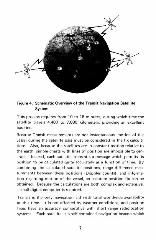
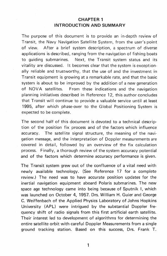
Figure 4. Schematic Overview of the Transit Navigation SatelliteSystem
This process requires from 10 to 16 minutes, during which time the
satellite travels 4,400 to 7,000 kilometers, providing an excellentbaseline.
Because Transit measurements are not instuntaneous, motion of the
vessel during the satellite pass must be considered in the fix calcula
tions. Also, because the satellites are in constant motion relative to
the earth, simple charts with lines of position are impossible to gen
erate. Instead, each satellite transmits a message which permits its
position to be calculated quite accurately as a function of time. By
combining the calculated satellite positions, range difference mea
surements between these positions (Doppler counts), and informa
tion regarding motion of the vessel, an accurate position fix can be
obtained. Because the calculations are both complex and extensive,
a small digital computer is required.
Transit is the only navigation aid with total worldwide availability
at this time. It is not affected by weather conditions, and position
fixes have an accuracy competitive with short range radiolocation
systems. Each satellite is a self-contained navigation beacon which
7

t 5
~SATELLITE
ORBIT
SHIPS MOTION DERIVED FROMDEAD RECKONING SENSORS(SPEED AND HEADING)
Figure 5. Geometry of a Satellite Pass
transmits two very stable frequencies (150 and 400 M Hz), timing
marks, and a navigation rnessage. By receiving these signals during a
single pass, the system user can calculate an accurate position fix.
There are two principal components of error in a Transit position fix.First is the inherent system error, and second is error introduced by
unknown ship's motion during the satellite pass. The inherentsystem error can be measured by operating a Transit set at a fixed
location and observing the scatter of navigation results. Figure 6 is a
plot of such data from a dual-channel Transit receiver showing a
radial scatter of 32 meters rms. Dual-channel results typically fall
in the range of 27 to 37 meters rms. Less expensive single-channel
receivers, which do not measure and .remove ionospheric refraction
errors, typically achieve results in the range of 80 to 100 meters rms.
The second source of position fix error is introduced by unknown
motion during the satellite pass. The exact error is a complex func
tion of satellite pass geometry and direction of the velocity error,
as explained in Chapter 6 of this document, but a reasonable rule is
8

..
LONG. = 1180 20' .260W
88.7 HOUR TEST69 INDIVIDUAL FIX RESULTS
70...--------------po-- ELEVATION ANGLES 150 -700
60 NO ALTITUDE ERRORNO VELOCITY ERROR
50 RMS ERROR = 32 METERS40 . MAXERROR=77METERS
30
20
en 10-~ 0 LAT. =33° 50' .465 Nw:2 -10
-20-
-30
-40
-50-60
-70
METERS
Figure 6. Typical Dual-Channel Satellite Position Fix Results
that 0.2 nautical mile (370 meters) of position error will result
from each knot of unknown ship's velocity. Figure 7 is a plot of
approximate position fix error as a function of unknown velocity
magnitude for dual-channel and for single-channel Transit receivers.
The effects of typical altitude errors and ship's pitch and roll have
been included in this curve as wei!.
Figure 8 illustrates the preferred mode of operation for a moving
navigator. Between satellite fixes the computer automatically dead
reckons based on inputs of speed and heading. The dead reckoning
process also is used to describe ship's motion during each satellite
pass. After the position fix has been computed, latitude and longitude adjustments are applied, thus correcting for the accumulated
dead reckoning error.
9
.10.05
~
~"",
~
~' //~~
~V
SINGLE CHANNEL~~ ~
~
~~
~~--- ---- ~~FIXED SITE
~~UAL CHANNEL---~~~ FIXED SITE
220
200en 180c::~ 160w~ 140
~ 120c::~ 100
x 80u..~ 60c:: 40
20
oo .15 .20 .25 .30 .35 .40 .45 .50
VELOCITY ERROR (KNOTS)
NOTES: 1. MAXIMUM SINGLE-CHANNEL FIX ERROR CAN REACH 200 TO500 METERS DUE TO IONOSPHERIC REFRACTION VERSUS ONLY90 METERS OF MAXIMUM FIX ERROR FOR DUAL-CHANNEL RESULTS.
2. SOLVING FOR VELOCITY NORTH CAN LIMIT FIX ERROR TO THERANG E OF 100-200 METERS WHEN VELOCITY IS POO RLY KNOWN.
Figure 7. Approximate Satellite Position Fix Error as a Functionof Unknown Velocity Magnitude
D. R. POSITIO\ ~ ...
."."".".""
.".""
--~.".--~~~~
SATELLITE FIXES
Figure 8. Dead Reckoning Error is Corrected by Each SatellitePosition Fix Update
10

CHAPTER 3TRANSIT APPLICATIONS
3.1 PRODUCT TRENDS
The Transit system provides a combination of capabilities whichcannot be obtained with any other system today. These are:
• Total global coverage
• All weather operation
• Accuracy approaching that of short range radiolocation
systems
• Independence from shore-based transmitters
• Unequaled dependability
As a result, there has been a steady and dramatic increase in both the
nUrTlber of applications and the types of equipment available. The
range of applications is truly surprisin~. Transit equipment is used
aboard and/or for:
• Land Survey
• Fishing boats
• Private yachts
• Commercial ships (tankers, freighters, etc.)
• Military surface ships
• Submarines
• Offshore dri II rigs
• Oil exploration vessels
• Oceanographic research vessels
• Hydrographic survey vessels
• Drifting buoys
To match the growing user interest and to take better advantage of
available technology, Transit user equipment has evolved dramati-
11

1978
AN/PRR·14
~~[~,
! MX·902 ANIWRN-S.__-------_-:-.::
t tMX·702CA " MX·702A
ANIWRN-4
Figure 9. Evolution of Magnavox Transit Receiver Technology
cally since the early equipment designs of 1967. Figure 9 is one view
of this evolutionary process, showing the many different types of
Transit receivers developed since 1967 by just one company.
Figure 10 is another view of the equipment progress, showing the
evolution of Magnavox single-channel satellite navigators from 1968
through 1976. In 1968 only dual-channel receivers were available,and a minicomputer occupied most of a rack. In 1971 a singlechannel receiver was introduced and by then minicomputers were
only 12 inches high. In 1973 the noisy, electromechanical Teletypewas replaced by a quiet and compact video terminal with a cassette
tape reader for loading the computer program. In 1975 new tech
nology permitted the receiver to be implemented on a pair of circuit
boards which fit within the computer. Also, minicomputers became
smaller, permitting greater freedom in the shipboard installation.
The final step in Figure 10 is the first production satellite navigator
based on microcomputer technology, the MX 1102. In addition to
being smaller, less expensive, and far more reliable than its predeces
sors, this new type of navigator also has more functional capability.
12

MX-702CA!hp1968
677-3646
I
J~.
MX-902!hp1971
MX-902!hp1973
"'
- I·1lI111.....1 .•"I
I
MX-902A1975
_.-=
MX-902B!hp1975
• -;1..~"
MX-11021976
Figure 10. Evolution of Magnavox Single-Channel SatelliteNavigation Equipment
For example, the MX 1102 not only tests itself thoroughly every two
hours, but it will identify which module to replace if a failure does
occur. Actual field results show a reliability of well over one year
mean time between failure (MTBF). Thus, modern technology has
lowered the cost and improved the capability of satellite navigation
instruments.
3.2 GENERAL NAVIGATION
Because of availability of instruments like the MX 1102 shown inFigure 11, general navigation applications of Transit have dramatical'ly increased in the last year or two. Such instruments provide acontinuous display of latitude, longitude, and Greenwich mean timeby continuously dead-reckoning between accurate Transit positionfixes with automatic speed and heading inputs. In addition to thebasic navigation functions, such systems determine and compensatefor unknown set and drift, provide great circle or rhumb line rangeand bearing to any selected way point, determine the heading tosteer to these way points, and in case of failure identify the faultymodule.
13

Figure 11. Magnavox Satellite Navigator MX 1102
Typical applications include use aboard large fishing vessels. For
example, when fishing for tuna in the southern hemisphere no other
navigation aid provides the coverage or the dependable accuracy
needed to assure success and to avoid fishing within 2DD-mile limits.
Success is measured by which boat returns first with full coolers,
and Transit navigation has measurably improved the rate of success.
Several large shipping companies in 1977 conducted competitive
evaluations of various types of navigation equipment (Loran, Omega,
and Transit, each from several manufacturers). Transit won each of
these evaluations, and as a result entire commercial fleets are being
equipped with Transit navigators: This trend is growing as the
economic and safety advantages of dependably accurate worldwide
navigation is proved over and over again. The availability of instru
ments with a low initial cost and with outstanding reliability records,
so that life cycle support costs are minimized, also has spurred
the interest of major fleet operators. The need for accurate, depend-
14

REMOTE VIDEO DISPLAY
DUAL CHANNELSATELLITE RECEIVER
DIGITAL COMPUTER
___~~~ PHOTOREADER
ANTENNAIPREAMPLIFIER
Figure 12. Typical Dual-Channel Equipment Used for Oceanographic Exploration
able, worldwide navigation is real. For example, oil tankers passing
through the Straits of Malacca truly depend on these characteristics.
Often a ship will time its arrival to obtain a satellite fix just before
proceeding through such hazardous waters.
3.3 OCEANOGRAPHIC EXPLORATION
The first application of Transit navigation beyond its original mili
tary objectives was for oceanographic exploration. For the first
time,mid-ocean scientific measurements could be tied to their geo
graphic origin with high accuracy. The AN/WRN-4 equipment
shown in Figure 9 and the equipment shown in Figure 12 are typical
of the dual-channel Transit systems often used for oceanographicexploration.
In addition to the capabilities provided by commercial single-channel
equipment, such as the MX 1102 of Figure 11, the dual-channel
equipment gives high accuracy position fixes that are unaffected by
variations in ionospheric refraction. In addition, it is typical for the
system to provide a printed record of the dead-reckoned position at
selected time intervals and of every satellite fix with appropriate
quality indicators.
The equipment described above is now yielding to the advent of
15

Figure 13. Magnavox MX 1107 Dual-Channel Satellite Navigatorand Printer
microcomputers. Figure 13 shows the Magnavox MX 1107 dual
channel satellite navigator with associated printer. This new instru
ment provides the same navigational accuracy capabilities as the
much larger equipment shown in Figure 12.
3.4 GEOPHYSICAL SURVEY
3.4.1 Background
In 1967 when Transit was first released for civil use, there were two
immediate positive responses. One was from the oceanographic
exploration community, and the other was from the offshore oil
exploration community. The oceanographers were among the first
civil users, but their needs have remained fairly static since the early
systems were acquired. In contrast, offshore oil exploration needs
have continued to grow and to become more complex.
Prior to 1967 all offshore exploration was conducted with the aid
of shore-based radiolocation systems such as Raydist, Hi-fix, etc.
These systems work very well, but they have several serious problems.
• Usable range is limited, especially at night.
• The administrative and logistics costs of obtaining govern
ment approvals, transporting the equipment, installing and
16

3.4.2 The Need for Integration
Transit provides intermittent position fixes with an individual accu
racy of 27 to 37 meters, but with an additional error of about
0.2 N.Mi. per knot of unknown velocity. Survey work requires the
high accuracy, but continuously. Thus, the only way to provide con
tinuous, accurate navigation independent of shore-based stations
was to combine accurate velocity sensors with the Transit fix capa
bility in an integrated system. The first such systems were relatively
crude, but very capable systems quickly evolved. Figure 14 shows
a typical integrated navigation system.
3.4.3 Doppler Sonar and Gyrocompass
The first system elements to be integrated were a Doppler sonar and
a gyrocompass. The Doppler sonar transmits pulses of acousticenergy to the ocean floor and evaluates the signals reflected back.
The Doppler frequency shift provides an accurate measure of ship's
speed with respect to the bottom in the direction of each sonar
beam. Three or four beams are used to determine both fore-aft and
port-starboard components of total velocity. An additional requirement is knowledge of speed of sound in water near the sonar trans
ducer. In most cases this can be determined to satisfactory accuracy
by measuring water temperature, but if salinity is likely to changedrastically, a velocimeter is required for best results.
17

SONARTRANSDUCER
Figure 14. Typical Integrated Navigation System Components
Early Doppler sonars were limited to about 200 meters of water
depth before they could no longer track the bottom and had toswitch to a water tracking mode, which is much less accurate. Theusual Doppler Sonar today will bottom track to 300 or 400 meters,
there are models available which will reach 1,000 meters or more,
and systems are being developed which promise bottom tracking tomaximum ocean depths.
Gyrocompasses such as the Sperry Mk-227 or the Arma Brown
MK-10 compass shown in Figure 14 have been used with good suc
cess. In both cases it is important to implement automatic computer
torquing of the gyrocompass to compensate for latitude, velocity,
and accelerations. Not only can the ~omputer do a better job than
would be possible with the usual manual control settings, but the
automatic approach avoids a major error source - the human mistake.
Navigational accuracy is dependent on a number of factors, including
complement of equipment, adequacy of calibration, water depth, andsea state. Figure 15 shows how position error grows with time
18

400
en 350a:wI-:g 300
2.01.8
150
200
250DEEPWATER OPERATIONWITHOUT LORAN-C
~Q\\\Q~c;,0\\ CO
~~~I\,Q~~\'-~ c;,,<S CO~Q\i\O~S
p..US ~I\ \lOO~ \. £ S'lS1£W\' 0 COMO\1
O~\ll£1 S1£~' GOOC AUSiERE S'l 000 CONOITIONS
~~==:::::::===::::::=------;C OMPLtTE S'lSTEM. G
50 NORMAL TIME BETWEEN FIXES=1TO 1.5 HOURS
Ol.--_~--"'--
o 0.2 0.4 0.6 0.8 1.0 1.2 1.4 1.6
TIME SINCE LAST SATELLITE FIX (HOURS)Figure 15. Integrated Sytem Error as a Function of Time Since
the Last Satellite Fix Updatesince the last satellite fix for a complete system and for an austere
integrated system under both good and poor conditions. The figure
also reveals how error increases much more rapidly when the sonar
cannot reach bottom, unless a radio aid such as Loran-C is available.
a:oa:a:wzoEeno0-en:2:a: 100
3.4.4 Radio Navigation Aids
In very d.eep water or where it is not possible to install a Doppler
sonar, some other source of velocity is needed. In many cases
various radionavigation signals may be available already. For
example, Figure 14 shows Loran-C components as part of the inte
grated system. Loran-C alone would not have sufficient accuracy
because of secondary phase errors and often because of poor IIcross
ing angles". However, by integrating Loran-C with other system ele
ments, excellent accuracy can be obtained. Satellite fixes provide
a precise geographic position reference and provide calibration of
local Loran-C secondary phase errors. By having a gyrocompass and
a Doppler sonar, even if in the water track mode, ship's maneuvers
can be determined accurately. This permits the Loran-C readings
19

to be filtered heavily, thus removing most of the random noise. In
effect Loran-C is used to correct for the effects of unknown set anddrift. Furthermore, because satellite fixes are available to provide an
accurate position reference, it is possible to use Loran-C in the
delta-range measurement mode with respect to a rubidium or cesium
clock. Because delta-range measurements can be made on each
Loran-C signal independently, useful information can be obtained
with only one or two Loran-C signals, which greatly expands the area
of accurate coverage and reduces the problem of poor crossing
angles.
The same concepts can be used with a wide variety of radionavi
gation systems. When integrating with short range, high accuracy
systems, a speed sensor is not needed, and the satellite fix capability:s used to verify and resolve lan~ counts. Systems have been implemented with such radionavigation aids as: Decca Navigator, Hi Fix,Raydist, Toran, Argo, Miniranger, Trisponder, and others. Each one
has its advantages, so flexible hardware and software is provided
for rapid configuration with any appropriate radio navigation sensor.
3.4.5 Acoustic Transponders
One of the most sophisticated versions of an integrated system
emp loys acoustic transponders (see References 14 and 15). The sh ip
is equipped \Nith an interrogater/receiver set. Every few seconds
the interrogator sends out an acoustic pulse at a specific frequency.
Transponders which have been placed on the bottom and are within
range receive the interrogate pulse and respond by sending a pulse
of their own at an individual frequency. The receiver on the ship
picks up and identifies these replies and measures the total round
trip delay. Such measurements, scaled with an appropriate estimate
of speed of sound in water, define the range to each transponder.
If the position of each transponder is known accurately, then a navi
gational accuracy of 2 to 10 meters can be achieved typically over an
area of 3 to 10 square kilometers with only a few bottom trans
ponders. Such systems are being used for site surveys and for precise
drill rig positioning during the final approach. Although expensive,
it may be the only way to achieve the required accuracy for 3-dimensional seismic surveys as well.
20

In the previous paragraph there was a big "if"; if the position of each
transponder is known accurately. This is the difficult part. Special
software has been developed to determine the transponder positions
with great accuracy and in a minimum of time. The first step is to
collect transponder range readings while following a specific pattern
around each transponder location. Because the equations must be
solved iteratively, these data are recorded in memory and used over
and over until the total solution converges and the relative position
of each transponder is known accurately. This technique saves time
by requiring the ship to traverse the area only once; the computer
does aII the work after that.
Once the relative transponder positions are known, it is often neces
sary to determine their true latitude and longitude positions as well.
This is achieved with the aid of multiple satellite position fixes.
Motion of the ship relative to the transponder net can be determined
accurately, but the position (translation) and azimuth (rotation)
of the net are unknown. Again, an iterative solution is used in which
each satellite fix improves knowledge of the net position and azi
muth. As knowledge of net azimuth improves, the measure of ship's
motion becomes more accurate. Such iterations are best done with
all raw satellite and transponder data recorded on magnetic tape, and
the technique has proved to be extremely effective and accurate.
3.4.6 Integrated Navigation System Functions
A wide variety of integrated navigation systems have been devel
oped and deployed to aid offshore exploration. However, naviga
tion is just one of the three major functions of an integrated system.
The other two are survey control and data logging.
The system helps control the survey, for example, by firing seismic
shots at defi ned increments of ti me or of distance traveled. In some
installati'ons the system actually controls steering of the vessel along
the desired survey path.
Data logging is the third necessary ingredient. Unless the position
at which the geophysical data were acquired is recorded, the dataare worthless. Therefore, data logging must be extremely reliable
21

result in 3-dimensions (latitude, longitude, and altitude). The geo
detic reference for such a rosition determination is provided by thesate II ite system itself.
If a reference station can be occupied within several hundred kilo
meters of a survey site, a technique called translocation can produce
greater accuracy in less time. To implement the translocation tech
nique, two or more satellite receivers are used, one at the reference
site and the other(s) at the survey site(s). By tracking the same satel
lite passes, improved accuracy is achieved because the computer
solves for differential position between the two points, which is not
affected by common error sources.
The U.S. Government conducts many surveys with Transit satellites.
The instrument normally used is the AN/P RR-14 Geoceiver shown
in Figure 16. For example, adjustment of the North American
Datum which is now underway depends heavily on results obtained
with the Geoceiver at many survey points across all of North
America. In reducing Geoceiver data, the Government has an advan
tage not available to the private user. This is postcomputation of
each satellite orbit based on data from tracking stations taken con
currently with the survey. The result is a "precise ephemeris" orbit
definition.
3.5.3 Equipment
Several different types of portable survey equipment have been
developed. The original, which is still in wide use, is the AN/PR R-14
Geoceiver shovvn in Figure 16. On the left is the four-frequency
receiver (which tracks both Transit and GEOS satellites), at the
center is the antenna and preamplifier on a tripod, and on the right
is the paper tape punch, which was the most reliable data recording
device when the design was completed in 1967. Magnavox has deliv
ered 55 Geoceivers which are used primarily by the U.S. Defenser~apping Agency for geodetic survey work. The Geocelver hasearned an enviable reputation for accuracy and for reliability.
Figure 17 shows the latest Magnavox instrument intended for fixed
point survey. It is called the MX 1502 Satellite Surveyor. Being
24

Figure 17. Magnavox MX 1502 Satellite Surveyor
25

compact and lightweight, it can be transported easily. In the field it
will operate for about three days on a 12-volt automobile battery.
During this time, the raw data from all satellite passes will be
recorded on a magnetic tape cassette. The cassette can be pro
cessed by a computing center for either point positioning or trans
location resu Its.
The MX 1502 does far more than simply record satellite data. It
computes and displays a 3-dimensional position fix result while in
the field. This result often may be adequate without post-process
ing the tape cassette, but in any case it is extremely valuable in
verifying proper system operation and assuring that the desired loca
tion has been occupied. In addition, the computed results help the
surveyor to know when sufficient data have been gathered so that he
can move to the next site with assurance. Assurance is a key ingre
dient of any survey system. Too often data are reduced to find that
something was wrong and that the site must be reoccupied at great
expense. The MX-1502 includes a thorough self-test capabil ity to
assure proper operation. If the self-test function detects a problem,
the specific module causing the problem is indicated. Repair by
replacement of plug-in modules allows the survey to continue with
minimunl disruption. Furthermore, after each record -is placed on
magnetic tape, it is immediately read back to assure no recording
rnistake. If an error is detected, that portion of data is re-recorded,
always assuring that the proper data are recorded correctly.
The MX 1502 can learn the orbits of all Transit satellites by reading
a previously recorded tape cassette. Thereafter, it will automati
cally go into a minimum power mode between satellite passes to
reduce battery consumption, waking up just in time to track only
the desirable passes. This new type of equipment will further expand
the application of satellites, both for marine and for land surveys.
3.5.4 Point Positioning Accuracy
A single satellite pass can be used to obtain a latitude and longi
tude position fix result. As described in Chapter 6 of this document
altitude must be defined, and an error in altitude can affect the posi-
26

5
4
~ 3w....w~Zo 2....::J....Joen....J«zu.:2:oa:u. 0zoi=~
~ -1o
-2
• LATITUDE
A LONGITUDEII ALTITUDE
110* HOURS OF TRACKING
-3
602010_41.-..JL-----------------........-----------
30 40 50PASS NUMBER
Figure 18. 3-D Point Positioning Convergence (62 MX 1502Satell ite Passes)
27

,. I I I , I I I • I I I I I @~221 I I I I
- 10 10 -21
~ -• • THREE DIMENSIONAL...... 25 10 FIX RESULTS (4/76)
~ NOTES:~
1) THE NUMBER OF PASSES- • IS INDICATED BESIDE- 50 • 51 EACH RESULT
- 77 ., 10 2) @ = WGS-72 GEODESY93 • = APL-4.5 GEODESY
- • 3) APPROXIMATE• • HORIZONTAL
I-- 10 26 25ACCURACY:
~ NO. PASSES METERS RMSI-- • 10 7I-- • 10 25 5f- lO~ -f- -
METERS-9 -8· -1 -6 -5 -4 -3 -2 -1 0 1 2 3 4 5 6 7 8 9 10 11987
6
5
4
32
~ 1w~ 0~ -1
-2-3-4-5
-6-7-8-9
Figure 19. 3-D Point Positioning Results
129
87
6
5
4
3
2
1 ~
o ~UJ
-1 ~
-2-3-4~5
-6-7
-8-9
tion fix accuracy. However, by processing multiple satellite passes
at one location, a 3-dimensional (latitude, longitude, and altitude)position fix can be determined. The best way to do this is with a
computer program which determines the one 3-dimensional position
that best fits all of the Doppler measurements obtained from all of
the satellite passes taken at that location. Figure 18 shows how a
typical 3-dimensional survey converges toward the final answer.
Each time another satellite is tracked, its data are combined with all
previous data and a new solution is computed. The figure indi
cates that with each successive satell ite pass, the latitude, longi
tude, and altitude parameters converge toward the final solution.
By conducting multiple convergence tests at the same location, one
can determine the repeatability of the final solution. As expected,
repeatability improves as the number of passes processed in each
solution increases. Figure 19 makes this clear. The number beside
28

each dot indicates how many passes were used for that position
fix, and it is evident that, for example, there is more scatter to the
10-pass solutions than to the 25-pass solutions. As tabulated on the
figure, the horizontal positioning repeatability is about 7 meters
rms with 10 passes and about 5 meters rms with 25 passes.
Figure 19 also illustrates another important concept, which is that
the position fix result is dependent on how the satellite orbits were
determined. Most of the data shown in the figure was obtained
before December 1975. In that month, the U.S. Navy changed the
basis for computing satellite orbits from one model of the earth's
gravity field to another (from APL-4.5 to WGS-72). The two points
which are circled in the upper right of the figure were determined
with the data taken after the conversion. Thus, we can use the
term "accuracy" only if we accept the satellite system as the basic
geodetic reference. Otherwise, it is proper only to describe therepeatability of such a process.
The results just described are available to every system user with the
necessary equipment and computer program. The principal source
of error is misknowledge of satellite orbital position, made worse
by the fact that orbit parameters in the satellite memory are a pre
diction of its position based on past tracking data. The predic
tion is obtained by numerical integration of the equations of motion,
taking into account all known forces acting on the satellite, such as
the gravity fields of the earth, sun, and moon, plus drag and radia
tion pressures. To the extent that these forces are not known pre
cisely, the predicted orbit will deviate from the actual orbit. These
differences account for most of the 27 to 37 meters rms of error
in individual Transit position fixes.
If the orbit did not have to be predicted into the future, a more
precise determination could be made, and the U.S. Defense Mapping
Agency (DMA) employs this technique in reducing satellite Doppler
data from survey receivers such as the AN/PRR-14 Geoceiver. Field
data are recorded on tape and returned to a computing center for
evaluation. There the Doppler data are combined with a precise
ephemeris of satellite positions based on tracked rather than predicted orbits; thus individual position fixes have a typical scatter of
29

only 6.3 meters rms. Naturally a 3-dimensional, multi-pass solution
converges to the required resolution much faster with this technique than when using predicted orbit parameters from the satellite.
However, the DMA seldom computes a precise ephemeris for more
than one or two satellites at a time, and immediate results cannot
be obtained in the field, offsetting slightly the advantage just
described. Even so, equipment using the predicted orbits must
remain on station from 4 to 10 times longer than equipment using
the precise ephemeris for equivalent accuracy results. The DMA has
shown 3-dimensional results with 1.5 meters per axis repeatability
after 25 precise ephemeris passes.
Precise ephemeris information is not available for commercial use.
However, there is precedent for the DMA to supply this information
to other nations based on cooperative international survey agree
ments.
Unfortunately, there is evidence that a precise ephemeris position fix
result will differ from one using data from the satellite message.
This difference is because the DMA uses a slightly different gravity
model to compute satellite orbits than does the Navy Astronautics
Group. This author regrets the difference and does not understandwhy it must persist.
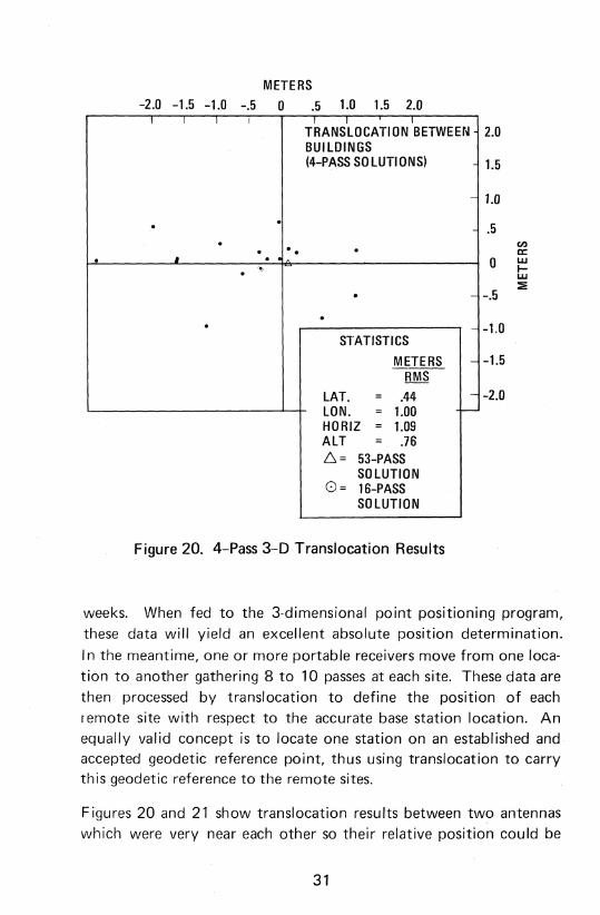
3.5.5 Translocation Accuracy
Although precise ephemeris data are not available commercially,
another technique called translocation can yield equivalent results.
Advantage is taken of the fact that almost all the error in a position
fix is caused by factors external to the satellite receiver. Thus, two
receivers tracking the same satellite pass at the same location should
produce nearly the same result (i.e., the errors are strongly corre
lated). Experience has shown that ·the correlation is quite effective
for interstation separations of 200 km or more. As a result, two or
more stations can be located with respect to each other with an
accuracy of 1 meter or better over very considerable distances.
One method of using translocation is to establish a base station
which collects data from all available satellite passes for days or
30
METERS
-2.0 -1.5 -1.0 -.5 0 .5 1.0 1.5 2.0I I I I I I I
TRANSLOCATION BETWEENBUILDINGS(4-PASS SOLUTIONS)
-
. .-. .. . .. , . .
'e/I~.
. -
.. -STATISTICS
METERS -
RMS
LAT. = .44 -
LON. = 1.00 -HORIZ = 1.09ALT = .76~= 53-PASS
SOLUTION0= 16-PASS
SOLUTION
Figure 20. 4-Pass 3-D Translocation Results
weeks. When fed to the 3-dimensional point positioning program,
these data will yield an excellent absolute position determination.
In the meantime, one or more portable receivers move from one loca
tion to another gathering 8 to 10 passes at each site. These data are
then processed by translocation to define the position of each
remote site with respect to the accurate base station location. An
equally valid concept is to locate one station on an established andaccepted geodetic reference point, thus using translocation to carrythis geodetic reference to the remote sites.
Figures 20 and 21 show translocation resu Its between two antennas
which were very near each other so their relative position could be
31

METERS-2.0 -1.5 -1.0 -.5 0 .5 1.0 1.5 2.0
I I I I I I I I
TRANSLOCATION BETWEEN-BUILDINGS(8-PASS SO LUTIONS) -
-
-.. .".. .. ..
STATISTICS -
METERS RSS
LAT. .21-
=LON. = .73HORIZ = .76 -
ALT = .47
6= 53-PASS SOLUTION--10= 16-PASS SOLUTION
2.0
1.5
1.0
.5CI.)
cc:0
wI-w~
-.5
-1.0
-1.5
-2.0
Figure 21. 8-Pass 3-D Translocation Results
determined with great accuracy. Each dot shows the difference
between the translocation result and the survey reference. All
satell ite passes above 15 degrees maximum elevation were used. For
this test, manual editing forced a balance of east and west passes for
the 4-pass solutions. For the 8-pass solutions, an imbalance of 5 vs 3
was allowed. Otherwise, all other editing was performed automati
cally. The horizontal accuracy was 1.09 meters rms for the 4-pass
solutions and 76 centimeters rms for the 8-pass solutions. This is
a measure of quality both of the computer program and of the I
receivers being used for the test. It should be noted that slightly
better results could be obtained through use of a rubidium or cesium
frequency standard at each receiver. Field tests indicate that this
level of translocation accuracy is obtainable over distances of several
hundred kilometers.
32

Figure 22. AN/WRN-5 Military Satellite Navigator
3.6 MILITARY APPLICATIONS
The Transit system was developed initially to provide precise posi
tion updates for the Polaris submarine fleet. In this application, a
submarine will expose its antenna at the appropriate time to update
and to maintain the accuracy of its inertial navigation systems.
l-ransit continues to be operated specifically to serve this Navy
appl ication .
u.s. Navy attack submarines also are navigated by Transit. Figure 22
shows the AN/WRN-5 satellite navigator which was developed for use
aboard nuclear attack submarines, although more are now being
used aboard surface ships. A number of other Transit sets also are
being used to navigate attack submarines, including the MX 702A/HP
system shown in Figure 12 and, more recently, the MX 1102 SatelIite Navigator shown in Figure 11. In fact, several NATO navies haveexpressed interest in a combination Transit-Omega navigator implemented within the MX 1102 structure both for submarines and forsu rface sh ips.
33

Submarine applications require the Transit navigator to provide
satellite alert information so that appropriate times can be chosento expose the antenna. In addition, it is desirable to minimize the
duration of each antenna exposure. This requires a receiver such asthe MX 1102 which tunes to the proper satellite frequency auto
matically, otherwise some provision for manual tuning must be
provided.
Rather than tracking only selected satellite passes, surface shipstrack every available satellite pass. The navigation concepts, appli
cations, and advantages are the same as for commercial ships, exceptthat accurate, worldwide, all weather navigation also provides tactical
and strategic advantages. Applications range from the navigation
of major combat ships to patrol vessels guarding the 200 mile eco
nomic zone boundary.
Transit is used extensively for military land survey and mapping pur
poses. The U.S. Defense Mapping Agency and many of the NATO
nations have cooperated on satellite survey operations across Europe.
Equipment such as the AN/PRR-14 Geoceiver, shown in Figure 16,
and the MX 1502 Satellite Surveyor, shown in Figure 17, can be
used for these purposes.
As Transit user equipment has become smaller, more reliable, and
less expensive, the opportunity for other land applications has been
created. Magnavox is investigating the application of Transit fixes
to vehicle positioning and even to manpack use. Although the time
interval between Transit fixes is not desirable, there are many situa
tions in which Transit could well be the only source of accurate
geographic reference. This is particularly true for vast desert or
jungle areas where accurately surveyed landmarks are not readily
available.
34

CHAPTER 4TRANSIT STATUS AND VITALITY
4.1 HISTORY AND FUTURE
Development of Transit began late in 1958, and the system became
operational in January of 1964. On July 29, 1967, then Vice
President Hubert H. Humphrey made an important announcement
as part of a speech at Bowdoin College. The key paragraph from
this speech reads as follows:
"This week the President approved a recommendation
that the Navy's Navigation Satellite System be made
available for use by our civilian ships and that commercialmanufacture of the required shipboard receivers be encouraged. This recommendation was developed by the Department of the Navy in support of initiatives of the Marine
Sciences Council to strengthen worldwide navigationalaids for civilian use. Our all-weather satellite system has
i been in use since 1964 by the Navy and has enabled fleetunits to pinpoint their positions anywhere on the earth.
The same degree of navigational accuracy will now be
available to our non-military ships."
The use of Transit has expanded greatly in the years since its introduction. Manufacturers around the world have taken the Presidential encouragement literally, and since 1968 when the first commer
cial Transit sets were available, there has been a steady and dramatic
increase in the types of equipment available and the number of users
worldwide.
Regardless of past achievements, however, questions are raised about
the future of Transit now that NAVSTAR, the Global Positioning
System (GPS) is being developed. If GPS achieves its developmentobjectives and operational funding is approved by the U.S. Congress,
it is reasonable to expect that Transit will be discontinued after asufficient overlap interval for users to depreciate existing equipmentand to select appropriate replacement GPS equipment. Althoughno policy statement has been published at this time, the availableinformation (see Reference 12) makes this author conclude that
35

1.-1f:I~,,*l~~:~I,W~/'~W~"~;1;JJ;i~
l~~~,r:~-,_....-,...~...--..-)~~~AN"E~~ ;.
Figure 23. The 5 Operational Transit Satellites, Launched on theDates Shown, are Backed by Twelve Reserve Spacecraftat RCA
Transit will be available until at least 1995. The following paragraphs emphasize the vitality of the Transit system today and forthe foreseeable future.
4.2 SYSTEM RELIABILITY AND AVAILABILITY
The Transit system reliability and availability can be seen in a num
ber of areas. One is the remarkable success rate of the Navy Astronautics Group in maintaining a proper orbit message in the memoryof each satellite. From January of 1964 to April of 1977, therehad been only 7 message injections which were not verified as
100 percent successful out of a total of 32,389 attempts. Each of the7 was corrected on the next satellite pass, about 107 minutes later.
This is a 99.98 percent success record and shows outstanding system
reliability.
36

Figure 23 expresses the satellite status in terms of reliability and
availability. Three of the five operational satellites were launched
over ten years ago at this writing. Amazingly, the signals are strong
and the satellites continue to function flawlessly. Backing up this
group of "never say die" performers are twelve spacecraft stored
where they were built many years ago at RCA Astro Electronics inNew Jersey.
Being very light (about 61 kilograms), Transit satellites can be placed
in their 1,100 kilometer orbits with relatively inexpensive, solid fuel
Scout rockets. Nine of these boosters currently are in reserve tosupport future launches.
It appears that Transit is in extremely good health when it comes to
reliable performance today and provision for continuation of service
for many years to come, especially noting the proveni-ongevity of
the spacecraft design.
4.3 NEW GENERATION OF SATELLITES
As shown in Figure 24, the Applied Physics Laboratory has devel
oped a new generation of Transit satellites, which they called TIP forTransit Improvement Program. Two prototype satellites were
launched as part of the development effort.
The Navy has decided to produce a limited number of these new
satellites, which will now be called NOVA. RCA is building the
first three NOVA satellites, and it is expected that at least two more
will be built. The first NOVA is expected to be launched in the
third quarter of 1979. This new satellite will be especially welcomein filling the orbit gap now existing between satellites 30120 and
30200,as discussed in Section 4.7.
The NOVA satellite signals are entirely compatible with the existing
Transit satellite signals. Therefore, all users will have access to this
new spacecraft. However, the NOVA satellites provide 'many impor
tant new capabilities, all of which have been verified with the experi
mentalTI P satellites. Of particular interest are the following:
• DISCOS, for disturbance compensation system, eliminates
37

Figure 24. New Generation NOVA Transit Satellite(Previously called TI PS)
the effect of atmospheric drag. As a result, each orbit
determination will retain accuracy for up to a week
instead of 24 hours now. With NOVA, we expect survey
navigation results to converge faster and have better
accuracy.
38

• NOVA is controlled by an on-board general purposedigital computer vvhich can be programmed from the
ground. In conjunction with a larger memory, the com
puter can provide orbit parameters for ten days withoutrequiring upload of new information.
• A new data modulation, transparent to existing receivers,
can be switched on. Plans for this modulation have not
been announced, but it could be used to provide more
precise orbit parameters.
• The received signal level from NOVA satellites will betwice as strong (3 dB). Antenna polarization will be
left hand circular on both channels rather than left on
150 MHz and right on 400 MHz at present.
• Very precise clock control has been achieved by permittingthe onboard computer to adjust oscillator frequency with a
resolution of about 1 x 10-12 (To make the carrier and the
data modulation coherent, the nominal frequency offset
has been changed from 80 ppm to 84.48 ppm, which
should not cause compatibility problems.)
• To transmit the precise time information, a high frequency
pseudo-random noise (PRN) modulation has been added
to both the 150 and 400 MHz signals. This also can be
used to achieve single-channel, refraction corrected fixes
(by detecting the difference in group delay and phase
delay effects), and a properly equipped receiver can blockout signals from any other satellite, thus eliminating the
potential for cross-satell ite interference.
4.4 EXPANDING USER BASE
Figure 25 is a chart prepared by the Navy Astronautics Group based
on information received from 15 of 19 manufacturers of Transit user
equipment. The chart shows a total user population of 1,899 sets
at the beginning of 1977, which was expected to grow to 4,350 sets
by the end of 1978.
39

737MILITARY
3000
5000 r-
N-
O-T-E-:-----r----------r--~11-4-60-D-U-A-L---,
INFORMATION BASED TOTAL 4350 CHANNEL4000 ON DATA RECEIVED FROM 2890 SINGLE
15 OF 19 MANUFACTURERS 3613 CHANNELCONTACTED
ena:~ 2000;::) 1899
1521
1000
378OL----------L--------~------~
1977 1978CALENDAR YEAR
Figure 25. Present Status and Expected Growth in Number ofTransit System Users (Provided by the NavyAstronautics Group)
The user population growth predicted by the manufacturers repre
sents an annual growth rate of 51 percent. To see if this were pos
sible, data was included from an earlier survey showing the total
population at the beginning of 1974 to be 600 sets. Growing from
600 to 1,899 in three years required an annual rate of 47 percent.
Thus, the predicted annual growth of 51 percent appears to be in
line with past trends, and it may be conservative when recent product innovations are considered.
Figure 25 shows the growth as a linear function of time, but includ
ing the data from 1974 tells us that this is not the case. In fact,the number of users has been increasing as a percentage of the exist
ing popul'ation, which is a straight line on logarithmic paper. Figure 26 is s·uch a plot using the three data points provided by the
Navy Astronautics Group. What may be surprising is that at present
rates the user population should reach 10,000 by the early 1980's.
Based on data available as of the first quarter of 1978, this growthtrend appears to be continuing.
40

10,0001974 1975 1976 1977 1978 1979 1980
10,000
~888 ~~0.-:: 90008000
7000 0° -':-- 7000"'0 --:-0\>''''6000 ~0\>'_-::'~~ 6000(/) 5000 \>'~ _-:-1°10 \>' ~~0 5000 (/)
~ 4000 \°10 - be O~ 4000 ~~ 3 00-(/) (/)
I.l. 3000 3000 I.l.0 0a: a:LiJ 2000 '2000 LiJco co~ ~:J ::>Z NOTES: Z
10001. 600 USERS RECORDED
1000900 900800 2. 1899 USERS RECORDED 800700 700600 3. 4350 USERS PREDICTED 600
Figure 26. Growth of Transit User Population Obtained From DataProvided by the Navy Astronautics Group
4.5 INVESTMENT IN TRANSIT NAVIGATIONEQUIPMENT
Combining data from the Navy Astronautics Group with other
sources, the total investment in Transit navigation equipment has
been estimated, as summarized by Figure 27. Research and develop
ment costs are not included, and equipment known to be out of ser-
" vice has been deleted. Overall, we believe the estimates are on the
low side.
The Navy Strategic Systems Project Office has been included as aseparate category due to their special involvement with Transit.
The total U.S. Government investment in Transit user equipment is
nearly 45 million dollars. Most of the integrated systems are owned
and operated by private firms engaged in offshore oil exploration.
The remaining dual-channel navigation systems are used for surveywork of various types, such as oceanography, land survey, drill rig
positioning, cable laying, etc. The single-channel navigators are usedfor general navigation purposes where 0.1 mile (fix accuracy is
sufficient, and this is the area of fastest growth.
41

AV. COST TOTAL COST WITH SPARESCATEGORY QUANTITY (THOUSANDS) (MILLIONS) (MILLIONS)
NAVY STRATEGIC SYSTEMS PROJECT OFFICE 73 -$ 251 $ 18.4 $ 23.9
U.S. GOVERNMENT - ALL OTHER 469 56 26.3 34.2
INTEGRATED SYSTEMS 118 231 27.3 35.5
OTHER DUAL-CHANNEL 539 47 25.2 32.8
SING LE-CHANNEL 2239 22 48.4 53.2
TOTALS 3438 $145.6 $179.6
Figure 27. Estimated Investment in Transit Navigation Equipment(April 1978)
The last column in Figure 27 is an estimate of the cost of equip
ment plus spares. Ten percent spares cost was assumed for the
single-channel equipment and 30 percent for all other categories.
Figures 26 and 27 carry a powerful and surprising message. It is
probable that at this time more money has been invested in Transit
user equipment than in marine equipment for any other U.S. radio
navigation system, including Loran-A, Loran-C, or Omega. Naturally
the reason for this has been the much higher price for Transit equip
ment, which always requires a computer and often is combined with
other sensors to form an integrated system. However, Figure 26
shows that the user population also is growing rapidly, spurred by
technical innovations which permit lower prices, better performance,
and greater rei iabi Iity.
4.6 COST OF TRANSIT SYSTEM OPERATION
The cost of operating Transit has been estimated by the Navy to be
as shown in Figure 28. For those familiar with the operational
costs of any other major navigation system, it should be obviolls
that Transit is very inexpensive to operate and to maintain.
4.7 IMPROVEMENT IN ORBITAL COVERAGE
Figure 29 shows the orbital spacing of the five operational Transit
satellites and their rates of precession as of March 23, 1978. This
specific orbital configuration was used to predict the average inter
val between satellite fixes given by Figure 3.
42

TRANSIT GROUND STATION
POINT MUGU, CALIFORNIA
PROSPECT HARBOR, MAINE
ROSEMONT, MINNESOTA
WAHIAWA, HAWAII
TOTAL
ANNUAL SUPPORT
TRANSIT GROUP SUPPORT
STORAGE OF 12 SATELLITES
SATELLITE REPLACEMENT COST
(INCLUDES SCOUT LAUNCHVEHICLE, SATELLITE CHECKOUTAND LAUNCH SUPPORT.)
PERSONNEL
152
20
28
9
209
ANNUAL COST
S 5.0 M
0.3
EACH
S 3.5 M
Figure 28. Cost of Operating the Transit System (Provided by theU.S. Navy, April 1977)
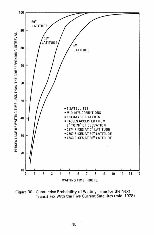
A better way to visualize the interval between fixes is that of Figure 30, which shows the cumulative waiting time probability at
three different latitudes. Note that intervals of more than 12 hours
occur infrequently at the equator, and intervals of six to seven hours
occur at higher latitudes. These peak values are strongly related
to the large gap between satellites 30120 and 30200 shown in Fig
ure 29, which is growing at about 5.1 degrees per year.
To evaluate the effect of filling the gap with another satellite, the
interval prediction program also was run with six satellites. The sixth
satellite is TRANSAT (30110), shown with a dotted line in Fig
ure 29, which was launched by the U.S. Navy in 1977. This satellite
is intended for purposes other than navigation, although it has a
Transit navigation mode which can be switched on if desired.
43

~
NORTH POLAR VIEW 2.1 o/VRMARCH 23, 1978
28.50 /YR
4.30 /YR
Figure 29. Orbitai Separation of the Five Operational TransitSatellites and TRANSAT (30110) on March 23, 1978
Figure 31, when compared with Figure 30, shows the dramatic effectof having a satellite in the orbit coverage gap. Not only are theremore satellite fixes available, but a much higher percentage occurafter shorter waiting times. Figure 32 show~ the effect on meantime between fixes of having TRANSAT.
Although having the gap filled would be very desirable, the Navy
does not plan to use TRANSAT in this way. However, as described
in Section 4.3, the Navy does plan to launch the new generation ofNOVA satellites beginning in the third quarter of 1979. Not only
44
100 I--------=:;:::;~::::=-------=:::::::====~
90...J«>a:UJI-Z
80c.!Jz0z00-en 70UJa:a:0uUJ:I:I- 60z«:I:I-enenUJ...J 50UJ:El- • 5 SATELLITESc.::J • MID-1978 CONDITIONSzi= 40 .153 DAYS OF ALERTS« • PASSES ACCEPTED FROM~ 8° TO 70° OF ELEVATIONu..0 .2274 FIXES AT 0° LATITUDEUJc.::J 30 • 2567 FIXES AT 30° LATITUDE« -4343 FIXES AT 60° LATITUDEI-zUJua:UJ0-
20
2 3 4 5 6 7 8 9 10 11 12 13
WAITING TIME (HOURS)
Figure 30. Cumulative Probability of Waiting Time for the NextTransit Fix With the Five Current Satellites (mid-1978)
45

100
300 LATITUDE90
...J«>a:w....
80zc.:Jz0z00- 70enwa:a:0(.)
W:I: 60....z«:I:....enen
50w...J
W:E....c.:Jz
40 6 SATELLITESi=~ (INCLUDES TRANSAT);: MID-1978 CONDITIONSu..
'53 DAYS OF ALERTS0UJ
30 PASSES ACCEPTED FROMc.:J« 80 TO 700 OF ELEVATION....
2729 FIXES AT 00 LATITUDEzw
309' FIXES AT 30° LATITUDE(.)
a:w 4797 FIXES AT 600 LATITUDE0- 20
, 0 0~---':'-~-~-~4-""""5L..---L6-......L.7_....Ja---1..9
-......;,'-0_...L,,--,.L..2
-....J'3
WAITING TIME (HOURS)
Figure 31. Cumulative Probability of Waiting Time for the NextTransit Fix Assuming TRANSAT Use (mid-1978)
46

100 ,...----------------------------.
5 SATELLITES
90
80
enw 70r-::::)
2
~Cf.)w 60~LL
2ww3= 50r-wcow:Ei=
402«w:E • MID-1978 CONDITIONS
• 153 DAYS OFALERTS30 • PASSES ACCEPTED FROM 8°
TO 70° ELEVATION ANGLES
20
70605020 30 40
LATITUDE (DEGREES)
10
10~---I.-_____L.._______I. ...L._._____L._______L.______'
o
Figure 32. Mean Time Between Fixes Which Would Occur With andWithout TRANSAT During mid-1978
47

399.968 MH~ [Z
OSCILLATOR~
FREQ MULT (~400 MHz)5 MHz - 80ppm X 80
I \V149.988 MHz
... FREQ MULT (~150 MHz)JII'" X 30
rPHASE '\VIr MODULATIONCLOCK....
FREQMEMORY 14- RECEIVER ~DIVIDE ...........
ADJUST9.6 JlSEC
Figure 33. Transit Satellite Block Diagram
will NOVA fill the gap, but the orbits will be controlled to maintain
precession at negligible levels. In 1980, two NOVA satellites with
orthogonal orbits will form the backbone of the Transit system, with
the existing satellites continuing to provide fixes as well.
4.8 SUMMARY
The preceding paragraphs have attempted to communicate the basic
vitality of the Transit system. We see this vitality in the system
reliability, the new generation of satellites, the expanding user base,
the amazing breadth of applications, the substantial worldwide
investment in Transit navigation equipment, and in the very low
cost of system operation. With all things considered, this author is
certain the Transit system will continue to provide its vital navigationservice until at least 1995.
48
CHAPTER 5THE POSITION FIX TECHNIQUE
5.1 THE SATELLITE SIGNALS
Figure 33 is a block diagram of the Transit satellite electronics.
The satellites transmit coherent carrier frequencies at approximately
150 and 400 MHz. Because both signals are derived by direct multi
plication of the reference oscillator output, the transmitted frequen
cies are very stable, changing no more than about 1 part in 1011
during a satellite pass. Thus, they may be assumed to be constant
with negligible error.
The reference oscillator output also is divided in frequency to drive
the memory system. In this waY,the navigation message stored
there is read out and encoded by phase modulation onto both the
150 and 400 MHz signals at a constant and carefully controlled
rate. Thus, the transmitted signals provide not only a constant ref
Arence frequency and a navigation message but also timing signals,
because the navigation message is controlled to begin and to end atthe instant of every even minute. An updated navigation message
and time corrections are obtained periodically from the ground byway of the satellite's injection receiver. The time correction dataare stored in the memory and applied in steps of 9.6 microsecondseach.
Each binary bit of the message is transmitted by phase modulation
of the 150 and 400 MHz signals. The modu lation format for abinary one is given in Figure 34, and a binary zero is transmittedwith the inverse pattern. As shown, this format furnishes a clock
signal at twice the bit rate, which is used to synchronize the receiv
ing equipment with the message data.
Because the satellites transmit only about one watt of power andmay be thousands of kilometers away, very sensitive receivers are
needed. In addition, however, the orbit parameters must be veri
fied by comparing redundant messages to detect and eliminateoccasional errors in the received data.
49

IBINARY ONE
~PERIOD~ 19.7 MSEC
POWER DIVISION
CARRIER 56.25%
DATA 37.50%
CLOCK 6.25%
------I SINE (cP)IIIIII
---+--IIII
IIIIIIIIIII
~--~-----------~
IIIIIIII
...-_..------ _-.J
~__..---------------.J III,
----~-------------------~COSINE (cf»
Figure 34. Transit Data Phase Modulation
5.2 INTERPRETATION OF SATELLITE MESSAGE
Figure 35 indicates how the navigation message defines the position of the satellite. During every two minute interval the satellite transmits a message consisting of 6,103 binary bits of dataorganized into 6 columns and 26 lines of 39-bit words, plus a final19 bits. The message begins and ends at the instant of the evenminute, which are denoted as time marks ti and ti+1. The final25 bits of each message form a synchronization word(0111111111111111111111110) that identifies the time markand the start of the next 2-minute message. By recognizing thisword, the navigation receiver establishes time synchronization andthereafter can identify specific message words.
50

11\\[
I.\ARK. t, cORBIT PARAMETERS
ll'i'l ,/ 11 '31
~:~~~ :::~ DEVIATIONS FROMll~E4 ---f-- 11 ELLIPTICALORBIT ------"'
llf\JE) 11-1 \ AT INDICATED TIMESLINEb II + ZLINE 7 II +)LINE'" -- -- --~f-"- 1
1+ 4
IIr-.,E q TIME OF PERIGEE
LINEIG MEAN MOTION
LINE 11 ANGLE OF PERIGEE
WJE ;Z PRECESSION OF PERIGEEII~E 13 I--- . __. __ ECCENTRICITY
II'Jl 14 1-- ~ .. ~.-f-- SEMI-MAJOR AXISLIM)) --f-- ANGLE OF ASCENDING NODEII"-Il lb PRECESSION OF NODE
LI~l .. "_1-_ COSINE OF INCLINATIONliM;' (,REENWICHLONGITUDE
IINE]O . ~ SATELLITE NUMBER
LINE ZO /o.\ESSAGE LOAD TIME
LINE 21 SINE OF INCLINATION
LI NE ZZ FREQUENCY OFF SET
LINE Z3 INJECTION FLAG
LINE Z4 INJECTION FLACLINEZ) INJECTIONFLAC.
LINE 26 '-----'4,--~'---'---'-r-I
liNE Z7 - \ 3q 81T WORDS L,.bl03 BITS I"J mo ',1INUTES Tlt"\f
1,1ARK!!.]
TWO MINUTE MESSAGE ORGANIZATION ORBIT DEFINITION
Figure 35. Satellite Message Describes Orbital Position
The orbital parameters are located in the first 22 words of column 6,and those in lines 9 through 22 are changed only when a new message is injected into the memory. These fixed parameters define asmooth, precessing, elliptical orb'it; satellite position being a function
of time since a recent time of orbit perigee.
The words in lines one through eight shift upward one place everytwo minutes, with a new word inserted each time in line eight.
These variable parameters describe the deviation from the smoothellipse of the actual satellite position at the indicated even minutetime marks. By interpolation through the individual variable param
eters, the satellite position can be defined at any time during the
satell ite pass.
Figure 36 aids in interpreting the Transit message parameters. Onthe left is a set of typical fixed parameters and an indication of howthey are to be interpreted. On the right is a set of variable parameters with an interpretation of one. The following paragraphs willdescribe how each of these is used.
51

1{kI
o = -0 5 = +01 = -4 6 = +12 = -3 7 = +23 = -2 8 = +34 = -1 9 = +4
INTERPRETATION
~270202748
"Q" NUMBER
*APPLIES TO PREVIOUS TIME MARK WHERE TIME IS IAN INTEGER MULTIPLE OF 4 MINUTES I
I
FIRST DIGIT OF 11k - - ---l
TYPICAL SATELLITEVARIABLE PARAMETERS
250512804260362810
~~~~~~~~-===:J 090072400
400182134410261833420321504430341164 __~---r_---l.~---,-_-""'_~---';::::::IIo....._....,
440330834000290534 -,
~~~~~~~: ~----:~--i----+""""I---+-------f
130020044 07 L -.0020 DEG L +2.74 KM -.08 KM *
BCDXS3 CODE MEANING OF FIRST DIGIT
0011 0 1000 5 0 ++0 5 +-10100 1 1001 = 6 1 +-0 6 -+10101 2 1010 7 2 -+0 7 --10110 = 3 1011 8 3 = --0 8 +0111 4 1100 9 4 ++1 9 =
049160940 I TIME OF PERIGEE =491.6094 MINUTES
836540260 [MEA[MOTION =3.3654026 DEG/MIN
815801870 IARGUMENT OF PERIGEE = 158.0187 DEG
800198330 [EATE OF CHANGE OF ABOVE =.0019833 DEG/MIN
800022690 I ECCENTRI CITY =0.002269
807464570 llEMI-MAJO R AXIS 7464.57 KM
803673600 @GHT ASCENSION OF ASCENDING NODE =36.7360 DEG
900002840 [RATE OF CHANGE OF ABOVE = -.0000284 DEG/MIN
800067000~ OF INCLINATION =0.006700
814855960 [RIGHT ASCENSION OF GREENWICH = 148.5596 DEG
809999780 [§INE OF INCLINATION =0.999978
TYPICALSATELLITE MESSAGEFI XED PARAMETERS
Figure 36. Interpretation of the Transit Message Parameters
vc
sp
EARTH CENTER Mk n (tk - tp)
SATELLITE POSITION Ek Mk + € SIN Mk +~ E(tk)
PERIGEE Ak Ao+~A{tk)
ME.AN ANOMALY uk Ak (COS (E k) - € )
ECCENTRIC ANOMALY vk AK SIN (Ek)
SEM I-MAJO R AX IS wk 17 (tk)
S
P
M
E
-+------.L..-----l-----!L--L..-~ uA ,?O
o~..-_//
MODIFIED TRANSIT ORBIT DEFINITION
=AoA
u{t) = A(COS E(t) - € )
v{t) =A)1 -€ 2SIN E (t)
w(t) IS UNDEFINED
CLASSICAL ORBIT DEFINITION
Mh) = nh-tp) 0
E{t) =M{t) + € SIN E(t)
Figure 37. u, v, w Satellite Coordinates are Earth-Centered andAligned with Perigee
The "Q" number provides a time tag for each word of the variable
parameters. In the example given, the number 07 nleans that th is
52

word applies at seven 2-minute intervals past the half hour, Le.,14 minutes or 44 minutes after the hour. This is why it is necessary
to initialize a Transit set to within plus or minus 15 minutes of cor
rect (GMT) time in order to synchronize properly. A time error
of less than 15 minutes will be resolved by the "Q"numbersfromthe satell ite message.
From Figure 36 also note that only one digit of the variable parame
ter 11k is transmitted in each word. Because two digits are required,
this parameter is defined only every four minutes at times which are
integer multiples of four minutes. The interpretation of the first
digit of 11k also is given by the figure.
The objective is to define the satellite position as a function of time.
To achieve this, three different coordinate systems are employed.
Figure 37 defines the u, v, w coordinate system. These coordinates
are earth-centered, u and v lie in the plane of the satellite orbit, andu is through the point of perigee (closest point to the earth). On theleft of Figure 37 are shown the classical Kepler orbit definition equations. The Transit orbit definition equations are very similar, except
for simplifications in the expressions for Ek and for vk. Error intro
duced by these simplifications is eliminated by application of variable
parameters ~Ek and ~Ak. The wk parameter defines out-of-plane
satellite motion, which is simply the variable parameter 11k.
Figure 38 shows how the x', y', z' coordinates are obtained by rota
tion of the u, V,W coordinates. Rotation by the "argument of peri
gee" places x' in the earth's equatorial plane.
Finally, Figure 39 shows that with two rotations the satellite posi
tion can be defined in an X, Y, Z coordinate system which is earthcentered and earth fixed, with Z being the polar axis (mean pole of
1900-1905 or Conventional International Origin) and X being in the
equatorial plane through the Greenwich meridian. The two rotations
account for the longitude of the orbit plane at tk and the inclinationof the orbit with respect to the earth's equatorial plane.
Figures 37 through 39 clearly show how the Transit orb,it parametersare interpreted and how they are used to obtain a definition of the
53

that the transmitted frequency is offset low by about 80 ppm(32 kHz at 400 MHz) to prevent f R from crossing 400 MHz.
The navigation receiver is equipped with a stable reference oscillatorfrom which a 400 MHz ground reference frequency f G is derived.Oscillator stability must be adequate to assume a constant frequencythroughout the satellite pass. As shown by the figure, the navigation
receiver forms the difference frequency fG-f R, and each Dopplermeasurement is a count of the number of difference frequency cycles
occuring between time marks received from the 'satellite. Because
every message bit effectively represents another time mark, theDoppler counting intervals are formed with respect to the messageformat of Figure 35. For example, each line of the message lasts
about 4.6 seconds, and the commonly used Doppler count interval
of 23 seconds is formed by starting a new count at the end of every
fifth line.
Each Doppler count is composed of two parts: the count of a constant difference frequency f G -fT , minus the count of the number of
Doppler cycles received during that time interval. It is the Doppler
cycle count which is physically meaningful. The count of the dif
ference frequency is an additive constant which is eliminated by the
position fix calculation.
Figure 40 emphasizes that the distance between the satellite and theobserver changes throughout the satellite pass. It is this change, infact, which causes the Doppler frequency shift. As the satellitemoves closer, more cycles per second must be received than were
transmitted to account for the shrinking number of wavelengthsalong the propagation path. For each wavelength the satellite movescloser, one additional cycle must be received. Therefore, theDoppler frequency count is a direct measure of the change in distance between the receiver and the satellite over the Doppler count
interval. In other words, the Doppler cou nt is a geometric measureof the range difference between the observer and the satellite at
two points in space, accurately defined by the navigation message.
56

This is a very sensitive measure because each count represents one
wavelength, which at 400 MHz is only 0.75 meter.
The equation defining the Doppler count of fG-f R is the integral
of this difference frequency over the time interval between receipt
of time marks from the satellite. For example,
(1 )
Note that t1 + R1/C is the time of receipt of the satellite timemark that was transmitted at time t1. The signal is received afterpropagating over distance R1 at the velocity of light C.
Equation 1 represents the actual measurement made by the satellite
receiver, but it is helpful to expand this equation into two parts:
+ R1/C(2)
Because the first integral in Equation 2 is of a constant frequency f G,it is easy to integrate, but the second integral is of the changingfrequency fRo However, the second integral represents the numberof cycles received between the times of receipt of two timing marks.
57

By a Jlconservation of cycles" argument, this quantity must equal
identically the number of cycles transmitted during the time interval
between transmission of these time marks. Using this identity,
Equation 2 can be written
+ R,/C
(3)
Because the frequencies f G and fT are assumed constant during a
satellite pass, the integrals in Equation 3 become trivial, resulting
in
Rearranging the terms in Equation 4 gives
(5)
Equation 5 clearly shows the two parts of the Doppler count. First
is the constant difference frequency multiplied by a time interval
defined by the satellite clock. Second is the direct measure of slant
range change measured in wavelengths of the ground reference fre
quency C/fG. It happens that the wavelength of f G is the proper
scale factor because received time marks are used to start and stop
the Doppler counts. If a ground clock is used to control the count
intervals, the wavelength of fT would become the appropriate
scale factor.
58

5.4 COMPUTING THE FIX
A usable satell ite pass wi II be above the horizon between 10 and
18 minutes, which determines the number of Doppler countsacquired. Typically 20 to 40 counts will be collected by modern
equipment. The Doppler counts and the satellite navigation mes
sage are passed to a small digital computer for processing. For
simplicity, we will assume a stationary receiver as shown in Figure 40
in order to establish the basic position fix concept.
The GO'mputer first takes advantage of message redundancy to eliminate errors in··the received orbit parameters. It is then able to com
pute the satellite's position at the beginning and end of every Dop
pler count. The computer also receives an estimate of the naviga
tor's. position in three dimensions, i.e., latitude, longitude, andaltitude above the reference ellipsoid. The equations of Figure 41
are used to convert the navigator's position into the same Cartesian
coordinate system shown in Figure 39, which permits the slant
range from the navigator to each satellite position to be calculated.It is then possible to compare the slant range change measured by
each Doppler count with the corresponding value computed from
the estimated navigator's position.
The difference between a Doppler measured slant range change
and the value computed from the estimated position is called aresidual e.. The objective of the position fix calculation is to find
Ithe navigator's position which minimizes the sum of the squares ofthe residuals (i.e., makes the calculated slant range change valuesagree best with the measured values). To implement the solution,a simplel linear estimate is made of the effect each variable willhave on each residual. Assuming we wish to solve for latitude (<1»,
longitude ("A), and the unknown frequency offset F = fG-fT, we
can write
A
e·I e· I
59
(6)

This equation states that if we move the estimated position by ~¢
and by b:.A and the estimated frequency offset by LlF, the presentresidual e. will become a new value, estimated to be e.. Next we wish
.I Ito minimize the sum of the squares of the estimated residuals by
setting the partial derivative with respect to each variable equal tozero. This results in three equations, where the summation covers
the m valid Doppler count residuals.
m
o~ Li=1
2 o
ooX
m
Li=1
A2e.I
2 Lm
( ae.)A Ie· .--
i=1 I oXo (7)
aaF
2
Ignoring all but the first-order terms of Equations 7 qives three
equations in the three selected variables, Lim, ~A, and .6F,
moej [e j
ae·6F1=L I aei 8ej-- D¢ - DA - 0a¢ a¢ GA. 8F
i= 1 .J
m[Je·
6F ]=[e jBe- 8ei DeiL • ,
ax 6¢ - 6A - aF 0 (8)a¢ 8A
l= 1
m1
L oei [ oe· Bel aej-- e· -- I L~cp - - 1\ A -- AF J=0of I a¢ aA aF
;=1
60

¢AHafbeRN
RN
XN
YN
ZN
LATITUDE
LONGITUDE
HEIGHT ABOVE ELLIPSOID
SEMI-MAJOR AXIS
FLATTENING COEFFICIENT
a( 1-f) = SEM I-MI NOR AXIS
V'"f(2-f) = ECCENTRICITY
RADIUS OF CURVATURE IN THE
PRIME VERTICALa/(1-e2 SIN 2¢)%
(RN + H) COS ¢ COS A(RN + H) COS ¢ SIN A[RN (1-e2) + H] SIN ¢
WGS-72 VALUES
(6378135 METERS)
(1/298.26)
(6356750.52 METERS)
Figure 41. Relating Latitude and Longitude to Cartesian Coordinates
Because only linear, first-order terms are used, the values of ~f/>,
6.A, and ~F which satisfy these equations will be an approximation
to the exact solution. Therefore, the original estimates of latitude,
longitude, and frequency are adjusted in accordance with the first
solution, and new slant ranges, residuals, and partial derivatives of
the residuals are computed for another solution. This process is
repeated, or iterated, until the computed values of dd>, dA, and
~F are sufficiently small, at which point the solution is said to
have converged. Normally, only two or three iterations are required,
even when the initial estimate is tens of kilometers from the final
solution. Note that ignoring higher order terms has no effect on
final accuracy, because these terms tend to zero as the solution
converges.
In summary, the Transit position fix begins with an estimatedposition and determines the shift in that position required to bestmatch calculated slant range differences with those measured by theDoppler counts. The initial estimate can be in error by 200 or
300 km and the solution will converge to an accurate value.
61

5.5 ACCOUNTING FOR MOTION
If the navigator IS In motion during the satellite pass, the moti'on
must be recorded before an accurate position fix can be computed.
As Figure 5 in Chapter 2 shows, only if the motion is known can the
calculated range differences from satellite to receiver be compared
properly with the range differences measured by the Doppler counts.
Aut9matic speed and heading inputs often are employed for this
purp,?se. During the satellite pass the computer creates a table
of the navigator's estimated latitude and longitude at the beginning
and end of each Doppler count interval. As before, the fix solution
provides a delta-latitude and a delta-longitude, which are added
to every point in the navigator's table between iterations of the
solution. Therefore, although the final position fix result may be
expressed as a latitude and a longitude at one point in time, the
fix solution in fact is a shift of the entire estimated track.
62

CHAPTER 6ACCURACY CONSIDERATIONS
6.1 STATIC SYSTEM ERRORS
Reference 11 presents an error budget for individual Transit position
fixes that provides a good summary of the factors affecting accuracy
when the navigator is not moving:
Source
1.
2.
3.
4.
5.
6.
7.
Uncorrected propagation effects (iono
spheric and tropospheric effects)
Instrumentation and measurement noise
(local and satellite oscillator phase jitter,
navigator's clock error)
Uncertainties in the geopotential model
used in generating the orbit
Uncertainties in navigator's altitude
(generally results in bias in longitude)
Unmodeled polar motion and UT 1-UTC
effects
Incorrectly modeled surface forces (drag
and radiation pressure acting on the
satell ites during extrapolation interval)
Ephemeris rounding error (last digit in
ephemeris is rounded)
Error
(meters)
1-5
3-6
10-20
10
0-10
10-25
5
S-ince publication of this table in 1973, the polar motion error has
been modeled and is included as an adjustment to the transmitted
orbit parameters. The root sum square (rss) of the remaining errors
lies in the range of 18 to 35 meters, which we believe is slightlyoptimistic due to the laboratory standards and the sophisticated
refraction correction models employed by the Applied Physics
Laboratory. Field results usually lie in the range of 27 to 37 meters
rss. Figure 6 presented a typical set of stationary fix results. The
63
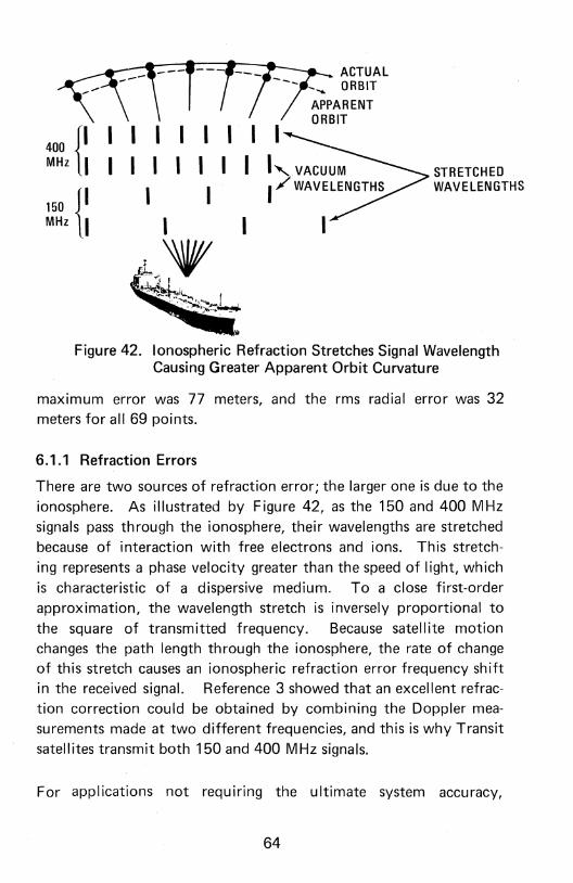
400 {IMHz I
150 {IMHz I
I I I I I II I I I I I
I II
t.'Vv: ~
-I. ~~t~~~.... !.~j~~
ACTUALORBIT
APPARENTORBIT
STRETCHEDWAVELENGTHS
Figure 42. Ionospheric Refraction Stretches Signal WavelengthCausing Greater Apparent Orbit Curvature
maximum error was 77 meters, and the rms radial error was 32meters for all 69 points.
6.1.1 Refraction Errors
There are two sources of refraction error; the larger one is due to the
ionosphere. As illustrated by Figure 42, as the 150 and 400 MHzsignals pass through the ionosphere, their wavelengths are stretchedbecause of interaction with free electrons and ions. This stretching represents a phase velocity greater than the speed of light, whichis characteristic of a dispersive medium. To a close first-orderapproximation, the wavelength stretch is inversely proportional tothe square of transmitted frequency. Because satellite motionchanges the path length through the ionosphere, the rate of changeof this stretch causes an ionospheric refraction error frequency shiftin the received signal. Reference 3 showed that an excellent refraction correction could be obtained by combining the Doppler measurements made at two different frequencies, and this is why Transit
satellites transmit both 150 and 400 MHz signals.
For applications not requiring the ultimate system accuracy,
64

.t'
.,
LONG. = 1180 20' .264 W
175 r-------------r------ 50 INDIVIDUAL FIX RESULTSELEVATION ANGLES 100 -700
150 NO ALTITUDE ERROR125 NO VELOCITY ERROR100 RMS ERROR =88 METERS75 MAX·ERROR =242 METERS
50 I(f.) 25~ 0 LAT. =33° 50' .465 Nw · -2 -25,
-50
-75-100
-125-150-175
L.-.-..J.---L---,-~I _ I I-250 -200 -150 -100 -50 0 50 100 150 200
METERS
Figure 43. Typical Single-Channel Transit Position Fix Results
400 MHz signal-channel receiving equipment can be used. Figure 42
demonstrates that because of wavelength stretching, the satellite
will appear to follow a path with greater curvature about the
navigator. The effect is to reduce the total Doppler shift somewhat,
pushing the position fix solution away from the satellite orbit to
explain the lower Doppler slope. Because the satellites move
primarily along north-south lines, the resultant navigation errors are
mostly in longitude. The magnitude of these errors varies with
density of the ionosphere from very small at night to peaks of 200 to
500 meters in daylight, depending on sunspot activity and location
with respect to the magnetic equator where the ionosphere is most
dense. Figure 43 is a plot of typical single-channel results containing
both daytime and nighttime fixes in which the maximum error is 242
meters and the rms error is 88 meters.
The second source of refraction error is the troposphere. In this
case, propagation speed is slowed as the signal passes through the
65

48
44
40
36
32
en 28a:w....w
24:?:
a:0ex: 20a:wwc.:J 16z«a:
12
8
4
o 10 20 30 40 50 60 70 80 90
ELEVATION ANGLE ABOVE HORIZON (DEGREES)
Figure 44. Typical Range Measurement Error Due to TrosphericRefraction
earth's atmosphere, which compresses the signal wavelength. The
effect is directly proportional to transmitted frequency, as is the
Doppler shift, and therefore it cannot be detected like ionospheric
refraction. There are only two ways to reduce the effect of tropo
spheric refraction. First is by modeling its effect on the Doppler
counts. Very sophisticated models employing measurements of tem
perature, pressure, and humidity have been published for this pur
pose, but less soph isticated models are usually sufficient (Ref
erence8). This is especially true in conjunction with the second
66

zI..LJ<q:
LONGITUDE -.J
DISPLACEMENT~ :=CQ0=o
ALTITUDE 2- - ---_'-..-J~-----~--""'",, j
X\ V"-
ALTITUDE 1
Figure 45. Effect of Altitude Estimate on Position Fix
technique,which is to delete Doppler data taken 'close to thehorizon where the tropospheric refraction error is greatest. Above
5° to 100 of elevation, the tropospheric error' is many times smallerthan at the horizon, as illustrated in Figure 44 which shows typicalmagnitude of range error as a function of elevation above the horizon.
6.1.2 Altitude Error
The specific Doppler curve obtained as a satellite passes is predominantly a function of the navigator's position along the line of satellite motion and his distance from the orbit plane. Because Transit
satellites are in polar orbits, the along~track position closely relates
to latitude and the cross-track distance is a combination of longitude
and altitude.
Figure 45 is the cross section of a pass where the satellite is moving
in its orbital plane perpendicular to the page. It has just reached the
center of pass with respect to stations X, Y, and Z. The figure illustrates how the cross-track distance is a function of both longitudeand altitude, which affect the Doppler curve in similar ways. Tocompute an accurate fix, therefore, it is necessary to have a prioriknowledge of altitude. Figure 46 shows the sensitivity of fix errorto altitude error as a function of maximum satellite pass elevation
67

1.0 Iex:~ 6.5
ffi 6.0
~ 5.5:::::>I- 5.0i=~ 4.5
~ 4.0c:~ 3.5
~ 3.0xu.. 2.5
~ 2.0oI- 1.5
~ 1.0
0.5 LATITUDE ERRORo
8D 70 60 50 45 40 35 30 25 20 15 10 6
MAXIMUM SATELLITE ELEVATION ANGLE (DEGREES)
Figure 46. Sensitivity of Satellite Fix to Altitude Estimate Error
angle. The elevation ang-Ie is plotted on a scale that is uniform in
probability of satellite pass occurrence. In other words, more passes
fall between 100 and 200 than between 700 and 800 , except at
very high latitudes.
For satellite navigation "altitude" means height above or below
the reference spheroid (the reference ellipsoid or satellite datum).
This surface is chosen to be a worldwide best fit to mean sea level,
which is the true geoid. Figure 47 illustrates the differences between
the geoid, the spheroid, and topography. Therefore, knowing height
above mean sea level is not sufficient for an accurate position fix.
One also must know the local geoidal height, which is the deviation
between the geoid and the spheroid. Figure 48 is a geoidal height
map indicating that these deviations reach nearly 100 meters.
68

A (SEMI-MAJOR AXIS)
en><«ex:oz~
I
~UJ
~aJ
/CENTER OFSPHEROID
'IJ = GEOCENTRIC LATITUDE
R GEOCENTRIC RADIUS
h = ELEVATION ABOVE GEOID
N = GEOID HEIGHT
<PA ASTRONOMIC LATITUDE
<PG GEODETIC LATITUDE
~ DEFLECTION OF THE VERTICAL
Figure 47. Relationships of Geodetic Surfaces (From NASADirectory of Observation Station Locations, 2nd Ed., Vol. 1,Nov. 1971, Goddard Space Flight Center)
69

LONGITUDE ERROR
~ .90a: .85~ .80~ .15~ .702>- .65
en !:: .6e'We..,:)
== 0 .55:aE u:: 50...J>'~ u. .45-0I- I- .40:::;)0<C 2 .352~
0:: .30~ .25~ .20cc .150::w.l0~ .05 LATITUDE ERRORLL.LL. OL..L_l-=:I::::::±~:::::!==:±=~t:::=:::::i~~±:::=====!=====~~=---.J
o 80 70 60 50 45 40 35 30 25 20 15 10 6MAXIMUM SATELLITE ELEVATION ANGLE (DEGREES)
Figure 50. Sensitivity of Satellite Fix to a One- Knot Velocity NorthEstimate Error
indicate realistic rms performance levels. One can see that a dual
channel system provides maximum benefit when there is an accurate
source of velocity. The other benefit of the dual-channel system is
to eliminate the peak 200 to 500 meter errors which occur with
single-channel equipment during the day, dependent on sunspot
activity.
6.3 VELOCITY SOLUTION
The normal position fix solution determines .Iatitude, longitude,
and frequency offset by means of Equations 8. These equations
easily could be expanded to include other system variables such
as velocity north, velocity east, altitude, and even acceleration.
With every new variable, however, accuracy would become more
and more sensitive to system noise. In fact, studies have shown
that velocity north is the only parameter which can be added without
72

660 50 45 40 35 30 25 20 15 10
MAXIMUM SATELLITE ELEVATION ANGLE (DEGREES)
a: .90~ .85~ .80tn .75~ .70~ .65
en c:; .60~~ .55i~ .50;;( ~ .45~~ .40~~ .35z a: .30~ .25~ .20~ .15~ .10u:: .05u.. OH--==:P-~-=:::::::~---+-+--+---::'::":":"':4-:-::'='=-+=":"::':'::~~---+--~
o 80 70
Figure 51. Sensitivity of Satellite Fix to a One-Knot Velocity EastEstimate Error
creating intolerable noise sensitivity; that is, it is the only other
variable which affects Doppler curve shape in a way that can be
discerned clearly from the effects of latitude, longitude, or fre
quency. To be precise, the added variable should be velocity
parallel to satellite motion, but velocity north is an adequate approxi
mation at most latitudes because the satellites are in polar orbits.
Solving for velocity north increases position fix error when ship's
motion is accurately known. Therefore it should be attempted only
when velocity errors are likely to exceed about 0.4 knot. The
expanded solution is more sensitive to other sources of system
noise, such as asymmetric Doppler data, and it does not work well
for pass elevation angles below 200 . Finally, the velocity northresu It becomes the scapegoat for other system errors and is not a
dependable measure of velocity north error; it simply allows the
latitude and longitude to be more accurate in the face of largevelocity errors.
73

6.4 REFERENCE DATUM
It is important to realize that maps are drawn and positions are
defined with respect to a reference datum. In the United States we
use the North American Datum, in Japan the Tokyo Datum, in
Europe the European Datum, etc. The Transit system currently
uses the World Geodetic System of 1972 (WGS-72). As a result, the
same reference marker will have a different set of latitude and
longitude coordinates in each reference datum. Apparent differ
ences of 1/2-kilometer occur in some locations.
The four parts of Figure 52 help us visualize the concept of reference
datums and how they relate to each other. Figures 47 and 48 already
indicated that the earth is an irregular shape due to density (gravity)
variations, and Figure 52(a)is an exaggerated model of an irregular
"earth". The surface shown represents the geoid, which is defined
asthe location of mean sea level over the entire earth's surface.
In order to make reasonably accurate maps, a model of the earth's
surface is needed. Figure 52(b) shows how such models have been
designed to fit the earth over the area of local interest, which in
the past never was larger than a continent. The model consists of
a spheroid (ellipsoid) and one position called the datum at which
latitude and longitude are defined. Such a model works well and
allows accurate maps to be drawn in the vicinity of the datum.
Now that satellites are being used to measure the geoid (satellite
geodesy), a different type of datum is needed. As illustrated by
Figure 52(c), a world spheroid may not fit the earth very well at
anyone location, but it is a "best fit" to the entire earth. In addi
tion, there is not a single reference datum position because many
satellite tracking stations are involved, and their positions are
defined as part of the calculations which determine the earth's
geopotential field (geoid). The vVGS-72 spheroid is a "best fit" to
the vVGS-72 geoid.
Figure 52(d) makes it clear that there must be some method of
relating a position in one datum to coordinates in another. For
74
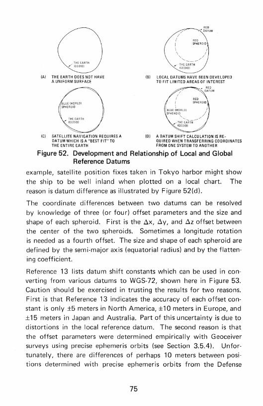
RED/ DATUM
REDSPHEROID
, THE EARTH,/ (GEOID)
(A) THE EARTH DOES NOT HAVEA UNIFORM SURFACE
(C) SATELLITE NAVIGATION REQUIRES ADATUM WHICH IS A "BEST FIT" TOTHE ENTIRE EARTH
;/"'
/I
II\ /\ /'" /"'-- /'---/- THE EARTH
(GEOID)
(B) LOCAL DATUMS HAVE BEEN DEVELOPEDTO FIT LIMITED AREAS 0 F INTE REST
(0) A DATUM SHIFT CALCULATION IS RE-QUIRED WHEN TRANSFERRING COORDINATESFROM ONE SYSTEM TO ANOTHER
Figure 52. Development and Relationship of Local and GlobalReference Datums
example, satellite position fixes taken in Tokyo harbor might show
the ship to be well inland when plotted on a local chart. The
reason is datum difference as illustrated by Figure 52(d).
The coordinate differences between two datums can be resolved
by knowledge of three (or four) offset parameters and the size and
shape of each spheroid. First is the ~x, ~y, and ~z offset between
the center of the two spheroids. Sometimes a longitude rotation
is needed as a fourth offset. The size and shape of each spheroid are
defined by the semi-major axis (equatorial radius) and by the flatten
ing coefficient.
Reference 13 lists datum shift constants which can be used in con
verting from various datums to WGS-72, shown here in Figure 53.
Caution should be exercised in trusting the results for two reasons.
First is that Reference 13 indicates the accuracy of each offset con
stant is only ±5 meters in North America, ±1 0 meters in Europe, and
±15 meters in Japan and Australia. Part of this uncertainty is due to
distortions in the local reference datum. The second reason is that
the offset parameters were determined empirically with Geoceiver
surveys using precise ephemeris orbits (see Section 3.5.4). Unfor
tunately, there are differences of perhaps 10 meters betweenposi
tions determined with precise ephemeris orbits from the Defense
75

SHIFTTOWGS-72
SEMI-MAJO R RECIPROCAL a =6378135DATUM SPHEROID AXIS FLATTEN ING 1If = 298.26
METERSMETERS 6X 6Y AZ
NAD 1927 CLARKE 1866 6378206 294.98 -2r 151' 176'
EUROPEAN INTERNATIONAL 6378388 297.00 -84 -103 -~TOKYO BESSEL 6377397 299.15 -140 516 673
AUSTRALIAN REFERENCE 6378160 298.25 -122 -41 146NATIONAL ELLIPSOID 1967
OLD CLARKE 1866 6378206 294.98HAWAIIAN
MAUl 65 -272 -197OAHU 56 -268 -187KAUAI 46 -271 -181
CAPE (ARC) CLARK 1880 6378249 293.47 -129 -131 . -282(MOD)
SOUTH REFERENCE 6378160 298.25 -77 3 -45AMERICAN ELLI PSO 10 1967
ORDNANCESURVEY AIRY 6377563 299.32 368 -120 425OF GREAT BRITAIN1936
JOHNSTON ISLAND INTERNATIONAL 6378388 297.00 192 -59 -211ASTRO 1961
f----
WAKE-ENIWETOK 1960 HOUGH 6378270 297.00KWAJALEI NATO LL 112 68 -44WAKE ISLAND 121 62 -22ENIWETOK ATOLL 144 62 -38
WAKE ISLAND ASTRO INTERNATIONAL 6378388 297.00 283 -44 1411952
CANTON ISLAND INTERNATIONAL 6378388 297.00 294 -288 -382ASTRO 1966
GUAM 1963 CLARKE 1866 6378206 294.98 -89 -235 254
ASCENSION ISLAND INTERNATIONAL 6378388 297.00 -214 91 48ASTRO 1958
SOUTH ASIA FISCHER 1960 6378155 298.30 21 -61 -15
NANKING 1960 INTERNATIONAL 6378388 297.00 -131 -347 0
ADINOAN CLARKE 1880 6378249 293.47 -152 -26 212
MERCURY 1960 FISCHER 1960 6378155 298.30NAD27AREA -25 46 -49ED AREA -13 -88 -5TO AREA 18 -132 60
MODIFIED MERCURY FISCHER 1968 6378150 298.301968
NAD27AREA -4 12 -7EDAREA -3 1 -6TO AREA 22 34 2
*VALUES OF -9,139, AND 173 SHOULD BE USED FOR ALASKA AND CANADA
Figure 53. Datum Shift Constants
Mapping Agency and those determined with orbits transmitted from
the Transit satellites. Figure 54, from Reference 13, gives the
Molodensky formulas most often used to transform coordinates from
one reference system to another.
76
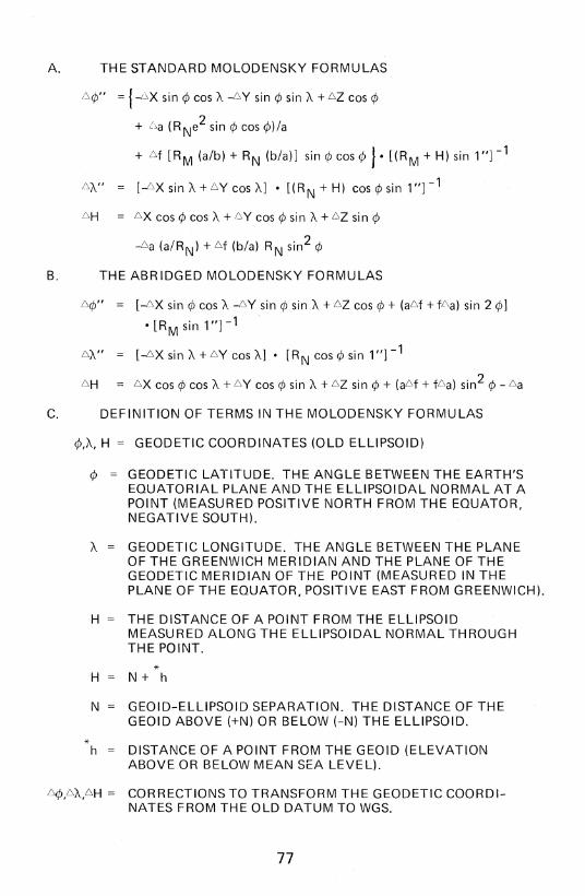
A. THE STANDARD MOLODENSKY FORMULAS
!~¢" = {-i',X sin ¢ cos A -6Y sin ¢ sin A + 6Z cos ¢
+ !:,a (R Ne2 sin ¢ cos ¢) la
+ 6f [R M (a/b) + RN (b/a)] sin rpcosrp}. [(RM
+ H) sin 1,,]-1
DA" [-6XsinA+6YcosA]· [(RN+H) cos¢sin 1,,]-1
LH 6Xcos¢cosA+6Ycos¢sinA+6Zsin¢
-6a (a/R N) + 6f (b/a) RN sin 2 ¢
B. THE ABR IDGED MOLODENSKY FORMULAS
6¢" = [-6X sin ¢ cos A -6Y sin ¢ sin A + 6Z cos ¢ + (a6 f + fL\a) sin 2 ¢]
[R . 1"]-1• M sin
6A" [-6XsinA+6YcosA]· [RNcos¢sin 1,,]-1
6H 6X cos ¢ cos A + 6Y cos ¢ sin A + 6Z sin ¢ + (a6 f + f6 a) sin2 ¢ - 6a
C. DEFINITION OF TERMS IN THE MOLODENSKY FORMULAS
¢,A, H = GEODETIC COORDINATES (OLD ELLIPSOID)
¢ = GEODETIC LATITUDE. THE ANGLE BETWEEN THE EARTH'SEQUATORIAL PLANE AND THE ELLIPSOIDAL NORMAL AT APOINT (MEASURED POSITIVE NORTH FROM THE EQUATOR,NEGATIVE SOUTH).
A GEODETIC LONGITUDE. THE ANGLE BETWEEN THE PLANEOF T,HE GREENWICH MERIDIAN AND THE PLANE OF THEGEODETIC MERIDIAN OF THE POINT (MEASURED IN THEPLANE OF THE EQUATOR, POSITIVE EAST FROM GREENWICH).
H THE DISTANCE OF A POINT FROM THE ELLIPSOIDMEASURED ALONG THE ELLIPSOIDAL NORMAL THROUGHTHE POINT.
*H N + h
N GEOID-ELLIPSOID SEPARATION. THE DISTANCE OF THEGEOID ABOVE (+N) OR BELOW (-N) THE ELLIPSOID.
*h DISTANCE OF A POINT FROM THE GEOID (ELEVATIONABOVE OR BELOW MEAN SEA LEVEL).
6¢,DA,6H = CORRECTIONS TO TRANSFORM THE GEODETIC COORDINATES FROM THE OLD DATUM TO WGS.
77
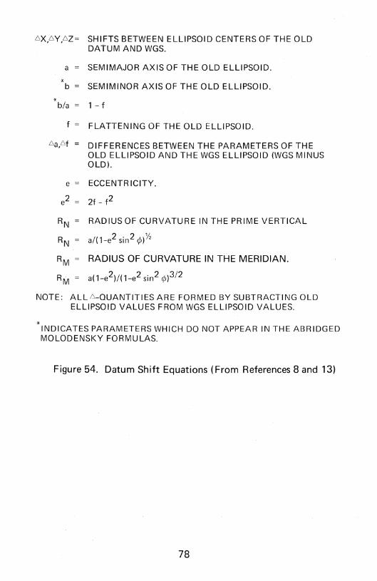
6X,6Y,6Z= SHIFTS BETWEEN ELLIPSOID CENTERS OF THE OLDDATUM AND WGS.
a = SEMIMAJOR AXIS OF THE OLD ELLIPSOID.
*b = SEMIMINOR AXIS OF THE OLD ELLIPSOID.
*b/a = 1-f
f = FLATTENING OF THE OLD ELLIPSOID.
6a,L\f = DIFFERENCES BETWEEN THE PARAMETERS OF THEOLD ELLIPSOID AND THE WGS ELLIPSOID (WGS MINUSOLD).
e = ECCENTR ICITY.
e2 = 2f - f2
RN RADIUS OF CURVATURE IN THE PRIME VERTICAL
RN a/{1-e2 sin2 ¢)Y2
RM RADIUS OF CURVATURE IN THE MERIDIAN.
RiVI a{ 1-e2 )/{ 1-e2 sin 2 ¢)3/2
NOTE: ALL6-QUANTITIES ARE FORMED BY SUBTRACTING OLDELLIPSOID VALUES FROMWGS ELLIPSOID VALUES.
* INDICATES PARAMETERS WHICH DO NOT APPEAR IN THE ABRIDGEDMOLODENSKY FORMULAS.
Figure 54. Datum Shift Equations (From References 8 and 13)
78

CHAPTER 7CONCLUSION
This document has provided an in-depth review of the Transit system
from the user's point of view. Except for a classified Soviet system,
Transit is the only navigation satellite system available today. Fur
thermore, because of propagation limitations of the Omega system,
Transit is the only system which provides truly worldwide coverage.
This situation will continue until at least 1985, or later, when
NAVSTAR, the Global Positioning System, is expected to become
operational. As proposed by the Office of Telecommunications
Policy (Reference 12), a ten-year overlap period from the time
NAVSTAR becomes operational will allow users to depreciate Transit
equipment before having to purchase NAVSTAR equipment. The
ten-year overlap also will give time for NAVSTAR manufacturers
to develop, improve, and produce a sufficient range of equipment
to serve the many expected applications (Reference 23). Thus, we
feel certain that Transit will continue to provide its most useful
service until at least 1995.
\iVe have shown that Transit is an extremely reliable system in
delivering accurate position fixes to its users. The reliability is
based on many factors. Signals are provided on a direct, line-of
sight basis from the satellite to the user, avoiding the propagation
problems that plague earth-based transmitters. The Navy Astro
nautics Group has established a remarkable record for maintaining
a reliable message in each satellite memory. The satellites them
selves are extremely reliable, with three which are operating
extremely well after more than ten years of service. The twelve
spacecraft in storage assure that the system can be maintained in
service for many years, even when the present satell ites cease to
function.
We have looked at the amazing breadth of Transit system applica
tions, ranging from use aboard fishing boats to military submarines.
If the user population growth trend continues, there will be more
than 10,000 Transit system users by the early 1980's. Comple-
79

menting the growth in applications and in the number of users is
development of a new generation of Transit satellite called NOVA.
Thus, there are many signs that the system is growing and fulfill
ing vital needs around the world.
Finally, this document has described both the theory of Transit
satellite navigation and the factors which affect accuracy perfor
mance. This has included a definition of the orbit message param
eters, the rneaning of the Doppler counts, and a review of theposition fix concept. The inherent system accuracy was described,
and sensitivity curves were given for external factors wh ich affect
position fix accuracy.
The primary objective of this document has been to provide an
extensive and detailed review of the Transit system today. A fasci
nating story has emerged. The system was developed almost exclu
sively to gu ide Polaris submarines, and it continues to serve th is
purpose extremely well. However, the U.S. Government also re
leased the system for commercial use, and on their own initiative
manufacturers around the world began to produce Transit navi
gation equipment. A wide variety of users are now experiencing
the advantages of accurate, worldwide, all-weather navigation. The
momentum of use continues to build, and Transit is destined to
playa vital role in the world navigation scene for another decade
or two.
80

SELECTED REFERENCES
1. Black, H.D. et ai, "Planned Improvements in the Transit
System (1975)", Navigation, Vol. 22, No.4, Winter
1975-76.
2. Etherington, M. "The Use of the Transit System in Tuna
Fishing", Marine Technology Symposium, United States
Trade Center, Mexico City, March 1977.
3. Guier, W. H. and Weiffenbach, G.C. "A Satellite Doppler
Navigation System", Proc. IRE, Vol. 48, No.4, April
1960.
4. Hatch, R.R. "Point Positioning and Translocation via
the Transit Satellite System", Magnavox Report MX-TM
3220-76, presented at The 46th Annual Meeting of the
Society of Exploration Geophysicists, Houston, Texas,
October 1976.
5. Hatch, R.R. "New Positioning Software from M,agnavox",
Magnavox Report MX-TM-3217-76, presented at the
International Geodetic Symposium on Satellite Doppler
Positioning, Las Cruces, New Mexico, October 1976.
6. Laurila, S.H. Electronic Surveying and Navigation, Chap
ter 28, John Wiley & Sons, 1976, ISBN 0-471-51865-4.
7. Leroy, C.F. JJResults from Portable Doppler Receivers
Using Broadcast and Precise Ephemerides", Proceedings
International Geodetic Symposium, Vol. I, co-sponsoredby U.S. Defense Mapping Agency, National Ocean Survey,NOAA, Las Cruces, N.M., October 1976.
8. Moffett, J.B. IJProgram Requirements for Two-Minute
Integrated Doppler Satellite Navigation Solution", Johns
Hopkins University Applied Physics Laboratory Report
TG 819-1 (Rev. 2), 1973.
9. Moyer, J.R. "Navigation and Positioning of Drill Rigs and
Other Offshore Platforms", Magnavox Report MX-TM
3248-77. Presented at Offshore Exploration Technical
Symposium, Gdansk, Poland, June 1977.
81

1 O. Moyer, J.R. "The Satellite Doppler Survey System - A
Modern Efficient Tool for the Field Surveyor", Magnavox
Report MX-TM-3247-77, Presented at the Seminar on
the Doppler System and its Application in the Determin
ation of Stations of Geodetic Control, Buenos Aires,Argentina, July 1977.
11. Piscane, V.L. et al /JRecent (1973) Improvements in the
Navy Navigation Satellite System", Navigation, Vol. 20,No.3, Fall 1973.
12. "Radio Navigation Systems Economic and PlanningAnalysis, Final Report'" Volumes 1, 2, and 3, Prepared
for Office of Telecommunications Policy by Computer
Sciences Corporation, July 1977.
13. Seppelin, T.O. "The Department of Defense WorldGeodetic System 1972", Defense Mapping Agency, Wash
ington, D.C., May 1974.
14. Sharpe, R.T. and Galyean, P.G. JJ An Acoustic Navigation
System for Site Survey and Geodetic Positioning", Magna
vox Report MX-TM,-3236-77, Presented at the Offshore
Technology Conference, Houston, Texas, May 1977.
15. Sharpe, R.T. /JAn Integrated Acoustic Positioning Sys
tem", Navigation, Vol. 24, No.3, Fall 1977.
16. Stansell, T.A. "The Navy Navigation Satellite System:
Description and Status", Navigation, Vol. 15, No.3,
Fall 1968.
17. Stansell, T.A. "Transit, The Navy Navigation Satellite
System", Navigation, Vol. 18, No.1, Spring 1971.
18. Stansell, T.A. "Accuracy of Geophysical Offshore Navi
gation Systems", Offshore Te.chnology Conference Pre
prints, OTC 1789, Dallas, Texas, April-May 1973.
19. Stansell, T.A. "Achieving Reliability in Automatic Navi
gation Equipment," Second International Symposium on
Ship Operation Automation, Washington, D.C., August1976.
82

20. Stansell, T.A. "Doppler Survey Equipment: Background,
Requirements and Trends" Magnavox Report
MX-TM-3219-76, Presented at the International Geodetic
Symposium on Satellite Doppler Positioning, Las Cruces,
New Mexico, October 1976.
21. Stansell, T.A. "Positioning and Navigation by Satellite",
Magnavox Report >MX-TM-3261-77, Joint Conference on
Satellite Applications to Marine Operations, New Orleans,
Louisiana, 15-17 November 1977.
22. Stansell, T.A. liThe Many Faces of Transit", Navigation,
Vol. 25, No.1, Spring 1978.
23. Stansell, T.A. "Civil Marine Applications of the Global
Positioning System", Navigation, Vol. 25, No.2, Summer1978.
83