transient flow analysis using the method of ... · 64 twyman, j. (2018). transient flow analysis...

62

Twyman, J. (2018). Transient flow analysis using the method of characteristics MOC with five-point interpolation scheme. 24, 62-70

Transient flow analysis using the method of characteristics MOC with five-point interpolation scheme

John TwymanTwyman Ingenieros Consultores, Pasaje Dos # 362, Rancagua, Chile, [email protected]

Análisis del flujo transiente usando el método de las características con esquema de interpolación de cinco puntos Fecha de entrega: 25 de agosto 2017

Fecha de aceptación: 21 de agosto 2018

An original 2nd-order Method of Characteristics (MOC) which it works with a five-point interpolating scheme valid for solving the hyperbolic and quasi-linear partial differential equations that describe the transient flow phenomenon in pipelines is shown. The results obtained by both MOC 2nd-order and exact solution (MOC 1st-order) are compared. It is shown that MOC 2nd-order allows obtain near-to-exact results within a wide range of Courant numbers.

Keywords: artificial viscosity, Courant number, method of characteristics 2nd-order, water hammer

Se muestra una versión original del Método de las Características (MC) de 2do orden que trabaja con un esquema de interpolación de cinco puntos, válido para resolver las ecuaciones diferenciales parciales hiperbólicas y cuasi-lineales que describen el fenómeno del flujo transiente en redes de tuberías. Se comparan los resultados obtenidos por el MC 2do orden y la solución exacta (MC 1er orden). Se demuestra que el MC 2do orden permite obtener resultados cercanos a los exactos dentro de una amplia gama de números de Courant.

Palabras clave: viscosidad artificial, número de Courant, método de las características 2do orden, golpe de ariete

IntroductionWater hammer is a hydraulic phenomenon that it appears in pipe networks when flow is affected by some disturbance that it alters the flow velocity, such as the valve opening or closure, the relief devices failure, the pump start-up or shutdown, etc. Pressure fluctuations can cause serious damage in piping and hydraulic devices, which it can result in accidents and other consequences such as costs increase associated with water supply and water quality. For this reason, in transient flow analysis it is very important to know about the pressure waves and about the prevention or minimization of their undesirable effects. Wave analysis is a vital task that it must be included in the water supply systems design to ensure their safety and reliability in emergency conditions, and also to detect obstructions, defects, leaks (losses) and pipe wall damages (Duan et al., 2014). Ignoring the water hammer effects may lead to erroneous pipe wall thickness’ dimensioning during the design stage. Transient flow phenomenon is difficult to understand intuitively, although the current computers

have allowed its automatic calculation -by means of numerical schemes- in systems with different complexity levels. The Method of Characteristics (MOC) has been widely used for transient analysis (Chaudhry and Hussaini, 1985; Chaudhry, 2013), where the equations governing the phenomenon are transformed into ordinary differential equations that can be solved through characteristic lines using finite-difference approximations. For numerical stability reasons, the Courant number (Cn) must always be less than or equal to 1.0; Cn = aΔt/Δx , where a is the wave speed, Δt the time step and Δx = LP/N is the reach length with LP the pipe length and N the number of reaches. 1st-order methods yield satisfactory results when the friction factor is small and Cn = 1.0. In systems transporting highly viscous liquids or in systems with small diameter pipes, the simulation may become unstable even with Cn < 1.0. On the other hand, the interpolations to be applied whenever solved using the MOC with Cn < 1.0 tend to soften wave fronts, and disturbances due to flow changes travel at a greater speed than the correct one (Chaudhry and Hussaini, 1985),

63

Twyman, J. (2018). 24, 62-70

being necessary to apply alternative methodologies to overcome these disadvantages. Trikha (1975) recommends using different time steps for each pipe in order to obtain Cn = 1.0. Despite its advantages, this methodology requires interpolating at the pipe boundary nodes, which it is an error source when modelling complex boundary conditions. Wiggert and Sundquist (1977) propose an interpolation algorithm in the space (x) axis, which it has been widely used in water hammer programs because of its efficiency and ease of programming. Holly and Preissman (1977) present a more complex formulation based on a 4th-order two-point method that is significantly more accurate than other higher-order methods using interpolations based on the four or five-point calculation. Goldberg and Wylie (1983) present two interpolation schemes (one implicit and the other one explicit) that operate on the time (t) axis of the space-time grid, both capable of reducing the numerical dispersion when MOC is applied with Cn < 1.0. Shimada and Okushima (1984) present two 2nd-order methods based on the solution in series and Newton-Raphson that they deliver results quickly and efficiently by omitting trivial terms calculated within the truncation error. Swaffield and Maxwell-Standing (1986) cite the Everett method as appropriate to reduce the numerical attenuation associated with Cn < 1.0. This method must be applied in tandem with Newton-Gregory method to interpolate in the nodes near-to-pipe boundaries. Lai (1989) presents three multimodal-type schemes that combine implicit schemes with explicit ones in order to attenuate the numerical dispersion. Yang and Hsu (1990, 1991) propose an improved version of the Holly-Preissman scheme, which however it presents a greater cost in terms of computational time. Sibetheros et al. (1991) investigate MOC applicability in tandem with spline-type interpolation polynomials for the water hammer’s numerical analysis in a frictionless horizontal pipe, finding that spline curves application significantly improves overall accuracy respect to both the MOC (linear interpolation) and the explicit finite-difference scheme (2nd-order). However, the method becomes complicated when it is required to represent the spline boundary conditions, and it presents problems when the transient modelling in short pipes is required. Ghidaoui and Karney (1994) investigate interpolation methods and the Holly-Preissmann scheme. They use the equivalent hyperbolic differential equation concept that it allows evaluate the

numerical scheme consistency, providing a mathematical description of both dissipation and numerical dispersion independently of Courant. In addition, the analysis allows comparing alternative approaches, and it explains why high-order methods should be avoided. Karney and Ghidaoui (1997) propose a flexible discretization scheme where several interpolation schemes are combined with the method of wave-speed adjustments. This hybrid scheme includes interpolations in a secondary characteristic line that it minimizes the distance between the interpolated point and the original characteristic line.

The current article introduces an original MOC 2nd-order scheme with linear interpolation in the spatial axis valid for the water hammer analysis in pipe networks. The results obtained by both MOC 2nd-order and exact result with MOC 1st-order with Cn = 1.0, are compared. Equations governing the transient flow along with wave speed and MOC 1st-order formulation are extensively discussed in the classic books by Wylie and Streeter (1978), Chaudhry (1979) and Watters (1984). These topics can also be studied in recent articles by Twyman (2016a, 2016b, 2016c, 2017, 2018). Finally, it is possible to study how to pose and solve boundary conditions within the MOC’s context in Karney (1984) and Karney and McInnis (1992), so no further details will be given here.

Basic equations of the transient flowWhen analyzing a volume control is possible to obtain a set of non-linear partial differential equations of hyperbolic type valid for describing the one-dimensional transient flow in pipes with circular cross-sectional area (Chaudhry, 1979; Wylie, 1984):

where: (1) and (2) correspond to continuity and momentum (dynamics) equations, respectively. Besides, is the partial derivative, H is the hydraulic grade-line elevation, a is the wave speed, g is the gravity constant, A is the pipe cross-sectional area, Q is the fluid flow, f is the friction factor (Darcy-Weisbach) and D is the inner pipe diameter. The subscripts x and t denote spatial and time dimension,

64


respectively. Equations (1) and (2), in conjunction with the equations related with the boundary conditions of specific devices, describe the phenomenon of wave propagation for a water hammer event.

Wave speedThe more general equation to calculate the wave speed in fluids without air is (Twyman, 2016b; Wan and Mao, 2016; Wylie and Streeter, 1978):

where K is the bulk modulus of the water, ρ is the water density, e is the pipe wall thickness, K is the volumetric compressibility modulus of water, E is the elasticity modulus of the pipe, c1 is a factor related with the pipe support condition, generally equal to 1 ‒ u2 (u is the Poisson’s ratio of the wall material), which corresponds to pipeline anchored against longitudinal movement (Wylie and Streeter, 1978).

Method of characteristics MOCMOC is very used for solving the transient flow equations because it works with a constant wave speed and, unlike other methodologies based on finite difference or finite element, it can easily model wave fronts generated by very fast transient flows. MOC works converting the computational space (x) - time (t) grid (or rectangular mesh) in accordance with the Courant condition. It is useful for modelling the wave propagation phenomena due to its facility for introducing the hydraulic behaviour of different devices and boundary conditions (valves, pumps, reservoirs, etc.). According to Karney (1984) and Karney and McInnis (1992) the MOC proceeds by combining the dynamic and continuity equations together with unknown multiplier. Suitable chosen values of this multiplier allows the partial differential terms to be combined together and replaced by total differentials. When using the simplified governing equations, the result of this process is:

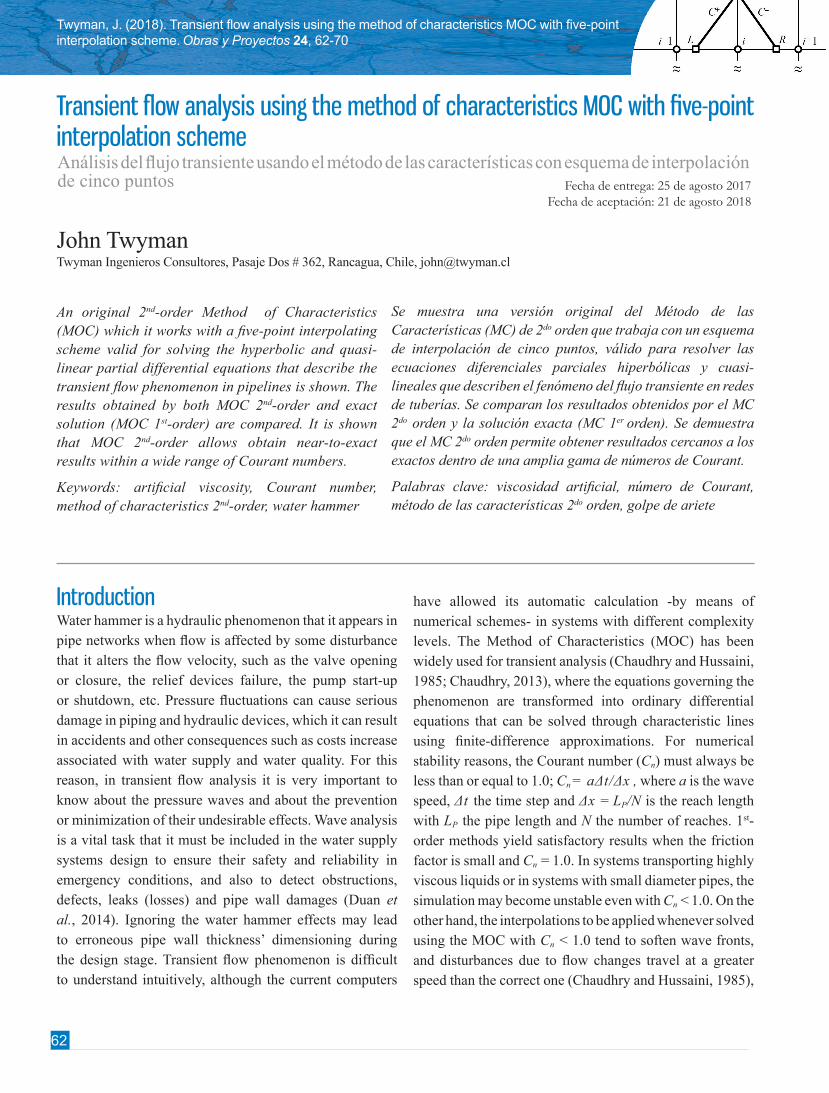
The two equations associated with the positive value are usually termed the C+ equations and the remaining two relations associated with the negative value are called the C - equations (Figure 1). The head and flow values are known at time t and it is desired to know these values at time t + Δt. A typical such point is P, with unknowns HP and QP. The known values at time t can correspond to initial state values or, instead, they can correspond to computed values at previous Δt. From Figure 1, Q and H are known in the nodes (i - 1) and (i + 1), and their new values must be calculated at node P. Due to this the characteristic lines are projected from P to the x-axis so as to be able to intercept it at points L and R. Because of xP and tP are specified by the analyst, L and R coordinates can be written as:

Figure 1: Space-time mesh for the specified time interval method

In order to calculate P the values in L and R must be known. However, only the grid point values in (i - 1) and (i + 1) are known. The values in L and R can be computed using linear (or higher order) interpolation schemes from the known conditions in (i - 1) and (i + 1). It is known that interpolations cause numerical dispersion and attenuation, which it has forced to apply more accurate high-order interpolation schemes whenever the pipe has Cn< 1.0 and when it is desired to leave unchanged the initial conditions of the problem (lengths, wave speed, etc.), or when there is a lack of a more stable numerical scheme than MOC. In MOC context, some analytic expressions can be obtained for the state variables at L and R nodes using numerical schemes with different interpolation orders (usually one or two). If U represents some state variable (H or Q), then the following expressions can be deduced according to Newton-Gregory interpolation scheme (i = 2,..., N)

65

Twyman, J. (2018). 24, 62-70

(Twyman, 2004):

with , U- =Ui-1 - Ui, U+ =Ui-2 - 2Ui-1+ Ui, U= =Ui+1 - Ui and U++ =Ui+2 - 2Ui+1+ Ui . Equations (8) and (9) are general since when Cn→0, UL→UR→Ui. When Cn = 1.0 the interpolation does not exist and UL becomes Ui-1 and UR

becomes Ui+1. On the other hand, when Cn = 2.0, UL becomes Ui-2 and UR becomes Ui+2. For this reason, the application of 2nd-order arrangements is sufficient to interpolate when the Courant number varies between 0 and 2.0. In this case the values for the variables U0 and UN+2 , both located beyond the nodes 1 and N + 1 respectively (Figure 2), they can be calculated by an extrapolation procedure defined by the following expressions:

Figure 2: Pipe nodes (adapted from Chaudhry and Hussaini, 1985)

where U1 and UN+1 are the values corresponding to upstream and downstream pipe sections, respectively. Once known UL and UR is possible to calculate HP and QP from the following formulas when U is equal to Q and H according to the convenience:

where c = (gA)/a and Rf = f/2DA. Equations (11) and (12) can be rewritten as:

with:

It should be noted that (16) is valid along the positive characteristic line C +and (17) is valid along the negative characteristic line C - . By simultaneously solving (14) and (15) it is possible to obtain HP and QP for all interior points P in the characteristic mesh:

once QP is known HP, value can be calculated from (14) or (15). For boundary sections an additional formula is required, which it must be solved together with the characteristic equation (positive or negative) depending on the position of the first or last reach, respectively. The calculation starts with an initial condition, usually steady-state flow.

Artificial viscosityArtificial viscosity (AV) is a fictitious mathematical term that it is introduced in the equations when working with finite differences, and it generates a similar effect to the real viscosity. The AV is a numerical technique that generates a fictitious attenuation over the spurious instabilities that frequently appear when fast transient flow is solved using 2nd-order numerical schemes. These instabilities generally appear in peaks form without physical meaning, and they may lead to destabilize the calculation due to equations nonlinearity (Brufau and García-Navarro, 2000). In other words, the phenomenon occurs when an approximate solution has an oscillatory and unrealistic behaviour respect to the analytical solution. In general, the precise cause of this effect is unknown, although it is known that they are generated when the first derivatives of the basic equations have more influence than the second derivatives or when the space-time grid is thick, with significant spacing between the nodes. Another cause could be the impossibility of the numerical schemes to capture all the discontinuities features, so there would be certain motion scales without numerical solution (Malekpour and Karney, 2016). The main difficulty of applying the AV lies in the dispersion amount determination needed to smooth (or

66


eliminate) the numerical oscillations without sacrificing the method’s accuracy level, and without unnecessarily affect the wave shape (Brufau and García-Navarro, 2000). The AV proposed in this paper recalculates H and Q every two time steps using the dissipation constant γ when the node i varies between pipe sections 2 and N, being the formula as follows (Abbott and Basco, 1989):

With U equal to Q or H as the case may be. In general, AV is easy to program and apply, although it has the disadvantage that its coefficient γ is difficult to estimate, being necessary to apply a trial/error procedure in order to determine its most suitable value. AV, independently of its shape, is an indispensable tool to suppress numerical oscillations (Hou et al., 2012) generated by high-order numerical schemes.

Results: example 1Water hammer is analyzed in a simple pipe network (Figure 3) using MOC 1st-order and 2nd-order. System includes a constant head reservoir (upstream end, node 1) with H0 = 100 m, a steel pipe and a valve (downstream end, node 2), where H0 = 98.1 m, being the pipe head loss due to friction Δhf equal to 1.9 m. The pipe data are: length LP= 4800 m, wave speed a = 1200 m/s, pipe cross−sectional area A = 3.14 m2, initial flow Q0 = 2.632 m3/s. Pipe network was discretized with N = 10. The friction factor (Darcy) is f = 0.022. Transient flow is generated by the valve closure in Tc = 35 s (Figure 4), and it can be considered as slow because the ratio 2(LP / a) = 8 s is much smaller than Tc.

Figure 3: Pipe network scheme (example 1)

For all effects the exact result is given by MOC 1st-order with Cn= 1.0. The maximum simulation time is Tmax = 60 s. Figures 5 and 6 show the envelopes for the maximum and minimum pressure heads obtained by MOC 1st-order and 2nd-order when the pipe is discretized in order to obtain the following Courant numbers: 0.2, 0.4, 0.6, 0.8 and 1.0,

which is achieved with the time steps Δt = 0.08, 0.16, 0.24, 0.32 and 0.40, respectively. For example, the value Cn = 0.2 results from the expression: aΔtN/LP = 1200 · 0.08 · 10/4800. Figure 5 shows that MOC 1st-order generates attenuations in the maximum pressure head that tend to decrease as Courant number grows toward the critical value Cn = 1.0. Figure 6 shows how MOC 2nd-order also generates attenuations, but on a smaller scale compared to 1st-order MOC as Cn moves away from 1.0.

Figure 4: Valve opening τ (%) versus time

Figure 5: Extreme pressure heads (MOC 1st-order)

Figure 6: Extreme pressure heads (MOC 2nd-order)

When Cn < 1.0, Figures 7 and 8 show that MOC 2nd-order is more accurate than MOC 1st-order. Regarding CPU

67

Twyman, J. (2018). 24, 62-70

execution times, the speed of both schemes is almost similar, with no significant differences (Figure 9). The examples were carried out in a standard PC with processing speed of 1.48 GHz.

Figure 7: Error (%) for maximum pressure head

Figure 8: Error (%) for minimum pressure head

Figure 9: CPU execution time.

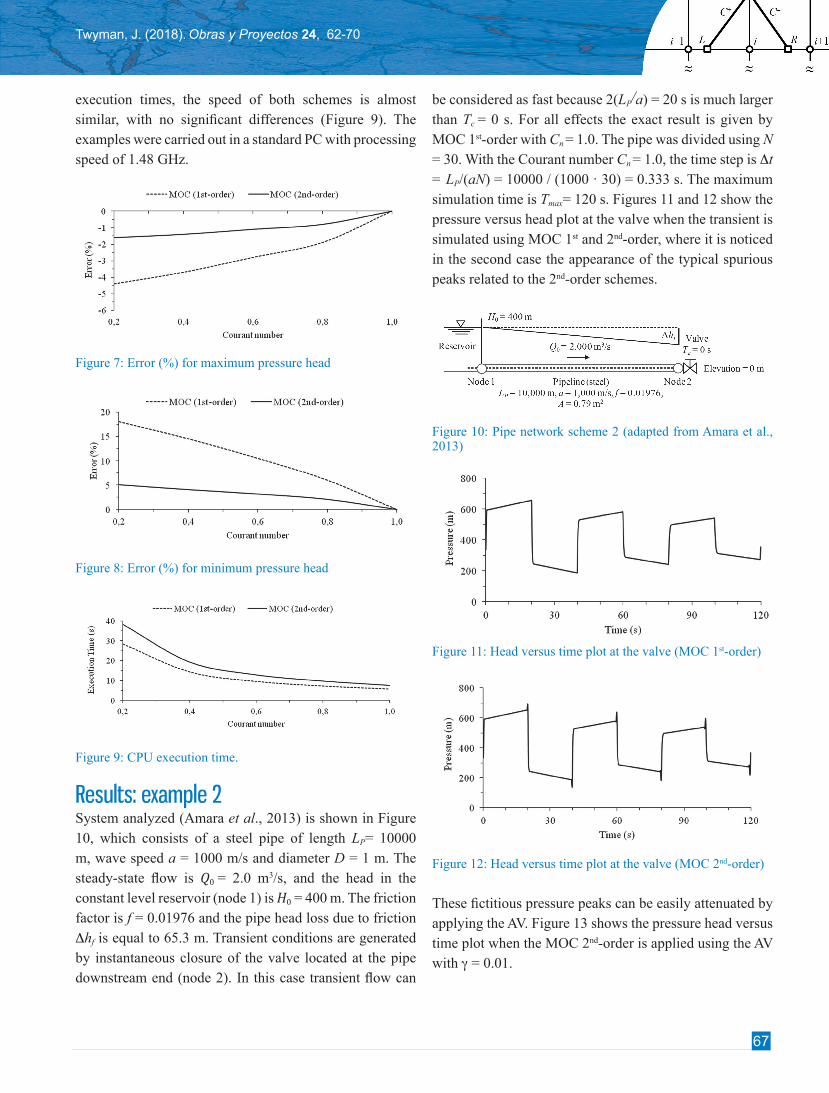
Results: example 2System analyzed (Amara et al., 2013) is shown in Figure 10, which consists of a steel pipe of length LP= 10000 m, wave speed a = 1000 m/s and diameter D = 1 m. The steady-state flow is Q0 = 2.0 m3/s, and the head in the constant level reservoir (node 1) is H0 = 400 m. The friction factor is f = 0.01976 and the pipe head loss due to friction Δhf is equal to 65.3 m. Transient conditions are generated by instantaneous closure of the valve located at the pipe downstream end (node 2). In this case transient flow can

be considered as fast because 2(LP/a) = 20 s is much larger than Tc = 0 s. For all effects the exact result is given by MOC 1st-order with Cn = 1.0. The pipe was divided using N = 30. With the Courant number Cn = 1.0, the time step is Δt = LP/(aN) = 10000 / (1000 · 30) = 0.333 s. The maximum simulation time is Tmax= 120 s. Figures 11 and 12 show the pressure versus head plot at the valve when the transient is simulated using MOC 1st and 2nd-order, where it is noticed in the second case the appearance of the typical spurious peaks related to the 2nd-order schemes.

Figure 10: Pipe network scheme 2 (adapted from Amara et al., 2013)

Figure 11: Head versus time plot at the valve (MOC 1st-order)

Figure 12: Head versus time plot at the valve (MOC 2nd-order)

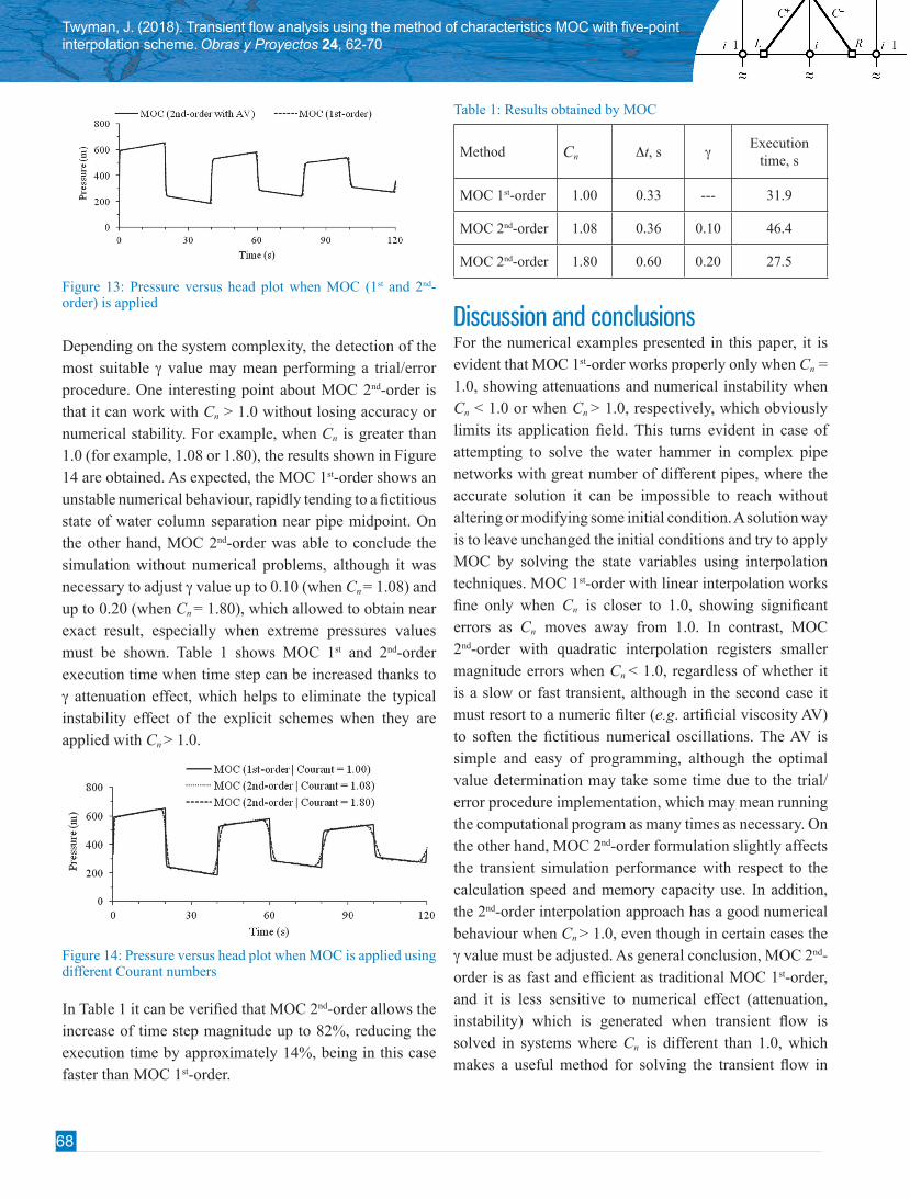
These fictitious pressure peaks can be easily attenuated by applying the AV. Figure 13 shows the pressure head versus time plot when the MOC 2nd-order is applied using the AV with γ = 0.01.

68


Figure 13: Pressure versus head plot when MOC (1st and 2nd-order) is applied

Depending on the system complexity, the detection of the most suitable γ value may mean performing a trial/error procedure. One interesting point about MOC 2nd-order is that it can work with Cn > 1.0 without losing accuracy or numerical stability. For example, when Cn is greater than 1.0 (for example, 1.08 or 1.80), the results shown in Figure 14 are obtained. As expected, the MOC 1st-order shows an unstable numerical behaviour, rapidly tending to a fictitious state of water column separation near pipe midpoint. On the other hand, MOC 2nd-order was able to conclude the simulation without numerical problems, although it was necessary to adjust γ value up to 0.10 (when Cn = 1.08) and up to 0.20 (when Cn = 1.80), which allowed to obtain near exact result, especially when extreme pressures values must be shown. Table 1 shows MOC 1st and 2nd-order execution time when time step can be increased thanks to γ attenuation effect, which helps to eliminate the typical instability effect of the explicit schemes when they are applied with Cn > 1.0.

Figure 14: Pressure versus head plot when MOC is applied using different Courant numbers

In Table 1 it can be verified that MOC 2nd-order allows the increase of time step magnitude up to 82%, reducing the execution time by approximately 14%, being in this case faster than MOC 1st-order.

Table 1: Results obtained by MOC

Method Cn Δt, s γExecution

time, s

MOC 1st-order 1.00 0.33 --- 31.9

MOC 2nd-order 1.08 0.36 0.10 46.4

MOC 2nd-order 1.80 0.60 0.20 27.5

Discussion and conclusionsFor the numerical examples presented in this paper, it is evident that MOC 1st-order works properly only when Cn = 1.0, showing attenuations and numerical instability when Cn < 1.0 or when Cn > 1.0, respectively, which obviously limits its application field. This turns evident in case of attempting to solve the water hammer in complex pipe networks with great number of different pipes, where the accurate solution it can be impossible to reach without altering or modifying some initial condition. A solution way is to leave unchanged the initial conditions and try to apply MOC by solving the state variables using interpolation techniques. MOC 1st-order with linear interpolation works fine only when Cn is closer to 1.0, showing significant errors as Cn moves away from 1.0. In contrast, MOC 2nd-order with quadratic interpolation registers smaller magnitude errors when Cn < 1.0, regardless of whether it is a slow or fast transient, although in the second case it must resort to a numeric filter (e.g. artificial viscosity AV) to soften the fictitious numerical oscillations. The AV is simple and easy of programming, although the optimal value determination may take some time due to the trial/error procedure implementation, which may mean running the computational program as many times as necessary. On the other hand, MOC 2nd-order formulation slightly affects the transient simulation performance with respect to the calculation speed and memory capacity use. In addition, the 2nd-order interpolation approach has a good numerical behaviour when Cn > 1.0, even though in certain cases the γ value must be adjusted. As general conclusion, MOC 2nd-order is as fast and efficient as traditional MOC 1st-order, and it is less sensitive to numerical effect (attenuation, instability) which is generated when transient flow is solved in systems where Cn is different than 1.0, which makes a useful method for solving the transient flow in

69

Twyman, J. (2018). 24, 62-70

pipe networks where its shape and configuration makes very difficult or impossible to fulfil with the Courant condition in all pipe sections.

ReferencesAbbott, M.B. and Basco, D.R. (1989). Computational fluid dynamics: an introduction for engineers. Longman Sc. & Tech., New York

Amara, L., Berreksi A. and Achour, B. (2013). Adapted MacCormack finite-differences scheme for water hammer simulation. Journal of Civil Engineering and Science 2(4), 226-233

Brufau, P. and García-Navarro, P. (2000). Esquemas de alta resolución para resolver las ecuaciones de “shallow water”. Revista Internacional de Métodos Numéricos para Cálculo y Diseño en Ingeniería 16(4), 493-512

Chaudhry, M.H. (2013). Applied hydraulic transients. Third edition. Springer, New York

Chaudhry, M.H. (1979). Applied hydraulic transients. Van Nostrand Reinhold, New York

Chaudhry, M.H. and Hussaini, M.Y. (1985). Second-order accurate explicit finite-difference schemes for waterhammer analysis. Journal of Fluids Engineering 107(4), 523−529

Duan, H.-F., Lee, P. and Ghidaoui, M. (2014). Transient wave-blockage interaction in pressurized water pipelines. Procedia Engineering 70, 573-582

Ghidaoui, M.S. and Karney, B.W. (1994). Equivalent differential equations in fixed-grid characteristics method. Journal of Hydraulic Engineering 120(10), 1159-1175

Goldberg, E.D. and Wylie, E.B. (1983). Characteristics method using time-line interpolations. Journal of Hydraulic Engineering 109(5), 670-683

Holly, M. and Preissmann, A. (1977). Accurate calculation of transport in two dimensions. Journal of Hydraulic Engineering 103(11), 1259-1277

Hou, Q., Kruisbrink A.C.H., Tijsseling A.S. and Keramat A. (2012). Simulating water hammer with corrective smoothed particle method. CASA-Report 12-14, Eindhoven University of Technology

Karney, B.W. (1984). Analysis of fluid transients in large distribution networks. PhD thesis, University of British Columbia, Vancouver, Canada

Karney, B.W. and McInnis, D. (1992). Efficient calculation of transient flow in simple pipe networks. Journal of Hydraulic Engineering 118(7), 1014-1030

Karney, B.W. and Ghidaoui, M.S. (1997). Flexible discretization algorithm for fixed-grid MOC in pipelines. Journal of Hydraulic Engineering 123(11), 1004-1011

Lai, C. (1989). Comprehensive method of characteristics for flow simulation. Journal of Hydraulic Engineering 114(9), 1074-1095

Malekpour, A. and Karney, B.W. (2016). Spurious numerical oscillations in the Preissmann slot method: origin and suppression. Journal of Hydraulic Engineering 142(3), 04015060

Shimada, M. and Okushima, S. (1984). New numerical model and technique for waterhammer. Journal of Hydraulic Engineering 110(6), 736-748

Sibetheros, I.A., Holley, E.R. and Branski, J.M. (1991). Spline interpolation for waterhammer analysis. Journal of Hydraulic Engineering 117(10), 1332-1349

Swaffield, J.A., Maxwell-Standing, K. (1986). Improvements in the application of the numerical method of characteristics to predict attenuation in unsteady partially filled pipe flow. Journal Research of the National Bureau of Standards 91(3), 149-156

Trikha, A.K. (1975). An efficient method for simulating frequency-dependent friction in transient liquid flow. Journal of Fluids Engineering 97(1), 97-105

Twyman, J. (2004). Decoupled hybrid methods for unsteady flow in pipe networks. Editorial La Cáfila, Valparaíso

Twyman, J. (2016a). Water hammer in a water distribution network. XXVII Latin American Hydraulics Congress IAHR, Spain Water & IWHR China, Lima, Peru, September 26-30

Twyman, J. (2016b). Wave speed calculation for water hammer analysis. Obras y Proyectos 20, 86-92

Twyman, J. (2016c). Water hammer analysis using method of characteristics. Revista de la Facultad de Ingeniería (U. de Atacama), 32, 1-9

Twyman, J. (2017). Water hammer analysis in a water distribution system. Ingeniería del Agua 21(2), 87-102

Twyman, J. (2018). Water hammer analysis using an implicit finite-difference method. Ingeniare: Revista Chilena de Ingeniería 26(2), 307-318

70


Wan, W. and Mao, X. (2016). Shock wave speed and transient response of PE pipe with steel-mesh reinforcement. Shock and Vibration 2016, article ID 8705031

Watters, G.Z. (1984). Analysis and control of unsteady flow in pipelines. Butterworths, Boston

Wiggert, D.C. and Sundquist, M.J. (1977). Fixed-grid characteristics for pipeline transients. Journal of Hydraulic Engineering 103 (13), 1403-1415

Wylie, E.B. and Streeter, V.L. (1978). Fluid transients. McGraw-Hill. International Book Company, USA

Wylie, E.B. (1984). Fundamental equations of waterhammer. Journal of Hydraulic Engineering 110(4), 539-542

Yang, J.C. and Hsu, E.L. (1991). On the use of the reach-back characteristics method of calculation of dispersion. International Journal for Numerical Methods in Fluids 12(3), 225–235

Yang, J.C. and Hsu, E.L. (1990). Time-line interpolation for solution of the dispersion equation. Journal of Hydraulic Research 28(4), 503–520

transient flow analysis using the method of ... · 64 twyman, j. (2018). transient flow analysis...

Documents