15Traffic Control and Traffic Managementin a Transportation Systemwith Autonomous Vehicles

Peter Wagner

15.1 Motivation

This paper aims to quantify the effects of autonomous driving on the traffic managementlevel. This involves developing a model of autonomous driving that makes it possible touse human-controlled and autonomous vehicles with only minor modifications. This isimportant with regard to defining how the instruments of traffic management need to bedeveloped in the future to enable them to handle autonomous vehicles in the transportationsystem. Of particular interest in this context is mixed traffic, in which normal and auton-omously driving vehicles interact with each other. This will presumably be the normal stateof affairs on roads for quite some time even after the introduction of autonomous vehicles;it is, therefore, of great practical significance to gain a good understanding of precisely thissituation to predict and prevent any systemic effects that may occur.

Since such vehicles do not yet exist, portions of the following observations must beregarded as an initial appraisal of possible developments presented as a scenario. How-ever, modeling of human drivers is likewise far from complete, so the focus in this paperwill be on establishing consistent modeling. The objective of the modeling presented hereis to describe, as far as possible, human and autonomous vehicles with the same model,distinguished only by the different parameters used. A good example of this is the distanceto the vehicle ahead expressed in terms of the time gap: an autonomous vehicle canachieve times of 0.3…0.5 s [1], whereas vehicles driven by humans are legally required tomaintain a distance of at least 0.9 s (in Germany). The legal recommendation is actually2.0 s, but this is seldom maintained except when traffic volumes are low. In heavy traffic,the value is often significantly lower; the figure for heavily traveled autobahns that occurs

P. Wagner (&)Institute of Transportation Systems, German Aerospace Centre (DLR),12489 Berlin, Germanye-mail: Peter.wagner@dlr.de

© The Author(s) 2016M. Maurer et al. (eds.), Autonomous Driving,DOI 10.1007/978-3-662-48847-8_15

301

most often is 1.1 s (see Fig. 15.3), with an average value of 1.4 s. If drivers complied withthe legally stipulated specifications, traffic on many roads would come to a standstill muchearlier than is currently the case.

This paper builds on the papers by Friedrich [2] and Pavone [3] in this book. While [2]describes the general effects of autonomous vehicles on the transportation system, thispaper addresses the modeling of autonomous and human-driven vehicles as well as theeffects of autonomous vehicles on traffic management. Paper [3], by contrast, largelyignores questions of traffic flow and traffic control and focuses primarily on the optimalallocation of supply in relation to demand based on the premise that vehicles can beshared. We can quite rightly conclude at this point that a combination of these approaches,together with a correct description of the share of travelers who would opt for trans-portation via a robotic “mobility-on-demand” system, allows the best possible appraisal ofthe potential of autonomous vehicles.

The paper also does not consider effects that would result from a fundamentally dif-ferent organization of transportation. One example of this would be the EU’s CityMobilproject, in which such scenarios are discussed and examined in greater detail [4].

This paper will examine how autonomous vehicles affect typical traffic managementapplications by looking at a few examples which have not been developed in all specifics.These examples, in order of increasing complexity, are the simulation of a single trafficsignal system (Sect. 15.4), simulation of an intersection controlled by an adaptive trafficsignal system (Sect. 15.5), simulation of a green wave (Sect. 15.6) and the simulation ofan entire city (Sect. 15.7).

Some of the questions to be considered here can draw on the effects of the introductionof intelligent speed control (autonomous intelligent speed control—AIC) on traffic flow onhighways in particular [5]. There is a great deal of literature on this subject; the disser-tation [5] and parts of the book [10] provide a more in-depth overview than is possible inthis chapter.

One such AIC scenario is highly similar to Use Case #1 “Interstate Pilot Using Driverfor Extended Availability”, which in turn (from a traffic-flow standpoint) is a specialvariant of Use Case #3, “Full Automation Using Driver for Extended Availability”. This isalso the use case that plays the most important role in this chapter, notwithstanding thefact that it is rather irrelevant from the traffic-flow standpoint whether the driver isavailable or not. The availability of the driver could be important if the impact of failureson traffic flow was being examined, but this topic will not be addressed in this book. Thiswould require detailed statistics regarding how frequently something of this sort occursand under what circumstances—information which is not available at the current stage oftechnology of autonomous vehicles. The Use Cases #2 (Autonomous Valet Parking) and#4 (Vehicle on Demand) play only a minor role in this chapter, although Use Case #4should be treated like Use Case #3 from a traffic-flow standpoint. Use Case #2 would beinteresting because it has an influence on parking search traffic and thus indirectly ontraffic demand and thereby also traffic control, but on the traffic management level itwould require a significantly more complex approach than can be achieved here—it would

302 P. Wagner

require, for example, a precise quantification of the parking search traffic in a city. Eventhe simulation of the city of Braunschweig described in Sect. 15.7 assumes that vehiclesthat have reached their destinations always immediately find a parking spot.

15.2 A Model of Driving

Models that describe how a human drives a vehicle have been around for a long time [6].Very many of these models (for an overview see [7–10])—since 1950 more than 100models have been described solely for the process of following a vehicle driving ahead—can also without further ado be applied as models for autonomous vehicles, albeit withdiffering parameters for humans and machines as mentioned in Sect. 15.1. It is thusconceptually quite simple to model mixed traffic and quantify its effects on the trans-portation system as a whole.

In the following, the focus will be on the process of following a vehicle, which is themost important, but not the only relevant process that determines the development oftraffic flow on roads.

Every vehicle is described by its position x(t), which depends on the time t and isdefined in relation to some reference (e.g. the beginning of the current section of road), byits velocity v(t) and its acceleration a(t); see also Fig. 15.1. In multi-lane traffic, the lane inwhich the vehicle is driving—the lateral coordinate, or distance of the vehicle from theedge of the road—comes in as a variable as well. Ideally each vehicle should also beindexed; this is circumvented in the following by describing the vehicle driving aheadwith uppercase letters X tð Þ;V tð Þ;A tð Þ. With the additional variables gap g tð Þ ¼ X tð Þ �x tð Þ � ‘ and difference in velocity Dv tð Þ ¼ V tð Þ � v tð Þ (see also Fig. 15.1), the reaction ofthe following vehicle can then be defined as the acceleration that the vehicle applies in aparticular situation:

a ¼ ddtv ¼ _v ¼ f v; g;Dvð Þ ð15:1Þ

This abstract Eq. (15.1) could be abstracted even further; lacking, for example, aremodels for driver errors and fluctuations as well as the modeling of a reaction time.A corresponding error model is introduced in Sect. 15.3, although reaction time, anotoriously thorny construct, is excluded entirely. While measurement data does very

( ), ( ) ( ), ( )( ), ( )

Fig. 15.1 Visualization of the applied dynamic variables using a SUMO [19] screenshot. Thetraffic direction is from right to left. Image rights: copyright resides with author

15 Traffic Control and Traffic Management in a Transportation … 303

frequently show that the acceleration of a following vehicle lags approximately 2 s behindthe acceleration of the vehicle driving ahead, there are also cases in which the followingvehicle starts braking approximately 1 s before the leading vehicle—for example whenapproaching a traffic signal (traffic light). In the following, we will examine the abstractEq. (15.1) with greater specificity. For example, one important question for the followingobservations is how precisely an autonomous vehicle moves. Surprisingly, many of thecurrent adaptive cruise control systems and also published control algorithms work forautomatic vehicles [11–13] as linear control systems:

_v ¼ a g� g� vð Þð Þþ bDv ð15:2Þ

Typical parameters for the two time constants are represented by a ¼ 1=20 1/s2 andb ¼ 1=1:5 1/s; with these values, cruise control systems are configured in a way that isperceived by drivers as agreeable and natural [14]. For the preferred gap g� vð Þ ¼ vs, as arule the legal regulation is applied, albeit with a somewhat smaller value for the preferredtime gap s, e.g. s ¼ 1:5 s, which is also used in the rest of this chapter. The model inEq. (15.2) was originally introduced in Helly 1959 [15] as a model describing a humandriver. This underscores the assertion that many driver models and the models forautonomous driving are mathematically very similar. Where they differ will be discussedin greater detail in Sect. 15.3.

The model in Eq. (15.2) has limits. For example, it is crash-free only for particularparameters ða; bÞ, and is only string stable for a small subset of parameters. String stabilityis the ability of a chain of vehicles driving behind each other not to succumb to the “slinkyeffect” and jam up: for instance, when minor braking by the first vehicle in the chain leadsto an amplified effect along the chain, in extreme cases actually causing a vehicle in thechain to come to a standstill. Or causing a traffic accident. To date, this behavior has onlybeen found in very specific situations (see [21] for an example)—it does not appear to bethe normal case.

However, the parameters with string stability are not perceived as very agreeable byhuman drivers, so AIC systems generally apply a compromise solution that results in aweak string instability [14].

For that reason, this paper looks at a different approach in the tradition of the models in[16–18]. A first step considers that an important condition for safe driving is fulfilled whenthe following applies:

d vð Þþ vs�D Vð Þþ g:

In this equation, D Vð Þ; d vð Þ are the braking distances of the leading and followingvehicles. Obviously this model is predicated on the following driver having an idea ofwhether and how the leading vehicle will drive or brake. That is certainly not entirelyadequate; and yet driving does work in many cases on the assumption that the otherdrivers will behave more or less as one does oneself.

304 P. Wagner

However, that also means that the approach flowing from this and the followingequation can be tricked by “strange” behavior on the part of the leading vehicle. If theleading vehicle has an autonomous emergency braking system that allows decelerationvalues of up to 12 m/s2, it violates the assumption of similar behavior to the followingvehicle—typical deceleration values for a human driver are in the range of up to max.4 m/s2—leading to a much shorter braking distance. This can be compensated for to someextent, as the following simulation results also show, because the equations resulting fromthis approach in the case of strong braking by the leading vehicle can exceed their owndeceleration. At the same time, this approach is one that could find further application inthe development of driver models for traffic safety.

The above model can be developed further by stipulating that the safety condition befulfilled not at the current time t, but also for a certain time t + T in the future. The timeT is the anticipation time, i.e. the length of the planning horizon of the driver. With thenotation x′ as a short-hand for the value of the variable x at the time t + T, the safetyequation becomes:

d v0ð Þ þ v0s�D V 0ð Þ þ g0:

But this equation can now be reformulated according to acceleration a. Thus x0 ¼xþ vT þ aT2=2 and together with an approach for the braking distances dðvÞ ¼ v2=ð2bÞ,the safety equation can be solved for a. There are various approaches for this; hereprimarily the following exact approach is pursued:

_v ¼ 1T

�b sþ T=2ð Þþffiffiffiffiffiffiffiffiffiffiffiffiffiffiffiffiffiffiffiffiffiffiffiffiffiffiffiffiffiffiffiffiffiffiffiffiffiffiffiffiffiffiffiffiffiffiffiffiffiffiffiffiffiffiffiffiffiffiffiffiffiffiffiffiffiffiffiffiffiffiffiffiffiffiffiffiffib2 sþ Tð Þ2 þV2 þ 2bvT þ 2b gþDvTð Þ

q� v

� �: ð15:3Þ

Interestingly, this approach for T ! 0 leads back to the one used in SUMO [19].Another possibility, following [17], is a Taylor expansion of

dðv0Þ ¼ dðvþ aTÞ � dðvÞþ aTv=bðvÞ, which, interestingly, leads to a linear equation fora which is simpler to solve and numerically less complex:

a ¼ V2 � v2 þ 2b TDvþ g� vsð ÞT 2bsþ bT þ 2vð Þ :

Although these equations look complicated, and it is rather unlikely that people canactually extract a root from a complex expression while driving, graphically it doesstrongly resemble the Helly model. This is interesting because it is indeed quite easy toimagine that a human driver is capable of carrying out a linear consideration along thelines of “I’m moving somewhat faster than the person in front of me, but the gap is large,so there is no immediate need to change anything.” An idea of how this accelerationfunction looks for realistically selected parameters is provided by Fig. 15.2.

15 Traffic Control and Traffic Management in a Transportation … 305

In this context it is also interesting to know whether this approach is indeed free ofcollisions. The simple answer is no. Under some circumstances, the dynamic that followsfrom Eq. (15.3) can indeed be fooled. This can be demonstrated by a chain of vehiclesfollowing a leading vehicle that is driving according to a specific protocol a0 tð Þ. Thesalient parameters in the dynamics of the leading vehicle are primarily the maximumaccelerations. Of particular interest here are the maximum decelerations and the questionas to whether it is possible to produce a collision with the model.

Of course, no procedure can really test all eventualities. But the following approachdoes at least allow an estimation of how secure the models are. In a simulation, n = 50vehicles follow a leading vehicle that selects its acceleration according to a specificprotocol. Among other things, it repeatedly decelerates to a standstill, in some cases withdecelerations at the limits of current driving dynamics capabilities. Studies on this set-upvery quickly revealed that collisions can only be avoided in the models when the antic-ipation time T during braking is set to a lower value. In the following the models arealways operated with T = 2 s in normal driving, and with T = 0.5 s when braking.

The respective simulations then show that, under these conditions, no accidents occurwith the model in Eq. (15.3), at least not with the selected protocol a0 tð Þ. The Hellymodel, however, is not so tolerant with the selected parameters and occasionally producesrear-end collisions.

-6 -4 -2 0 2 4 6

010

2030

4050

Δv (m/s)

g (m

)

-6 -4 -2 0 2 4 6

010

2030

4050

Δv (m/s)

g (m

)Fig. 15.2 Representation of the acceleration functions. Rather than drawing the entire functionhere, only the area delimited by two lines in the Dv; gð Þ range is represented, in which theacceleration of both models is small. To the left of the lines, the vehicle is braking, to the right it isaccelerating. The figure on the left is the model from Eq. (15.3), the one on the right the Helly model(15.2). The selected parameters are V = 20, τ = 1.5, b = 4, T = 2. Image rights: copyright resides withauthor

306 P. Wagner

15.3 Man Versus Machine

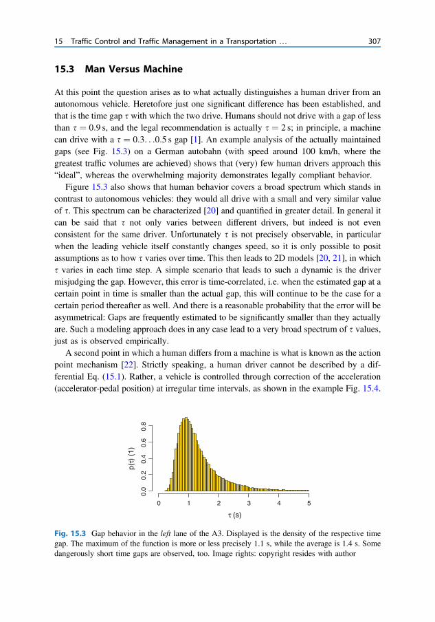
At this point the question arises as to what actually distinguishes a human driver from anautonomous vehicle. Heretofore just one significant difference has been established, andthat is the time gap s with which the two drive. Humans should not drive with a gap of lessthan s ¼ 0:9 s, and the legal recommendation is actually s ¼ 2 s; in principle, a machinecan drive with a s ¼ 0:3. . .0:5 s gap [1]. An example analysis of the actually maintainedgaps (see Fig. 15.3) on a German autobahn (with speed around 100 km/h, where thegreatest traffic volumes are achieved) shows that (very) few human drivers approach this“ideal”, whereas the overwhelming majority demonstrates legally compliant behavior.

Figure 15.3 also shows that human behavior covers a broad spectrum which stands incontrast to autonomous vehicles: they would all drive with a small and very similar valueof s. This spectrum can be characterized [20] and quantified in greater detail. In general itcan be said that s not only varies between different drivers, but indeed is not evenconsistent for the same driver. Unfortunately s is not precisely observable, in particularwhen the leading vehicle itself constantly changes speed, so it is only possible to positassumptions as to how s varies over time. This then leads to 2D models [20, 21], in whichs varies in each time step. A simple scenario that leads to such a dynamic is the drivermisjudging the gap. However, this error is time-correlated, i.e. when the estimated gap at acertain point in time is smaller than the actual gap, this will continue to be the case for acertain period thereafter as well. And there is a reasonable probability that the error will beasymmetrical: Gaps are frequently estimated to be significantly smaller than they actuallyare. Such a modeling approach does in any case lead to a very broad spectrum of s values,just as is observed empirically.

A second point in which a human differs from a machine is what is known as the actionpoint mechanism [22]. Strictly speaking, a human driver cannot be described by a dif-ferential Eq. (15.1). Rather, a vehicle is controlled through correction of the acceleration(accelerator-pedal position) at irregular time intervals, as shown in the example Fig. 15.4.

0 1 2 3 4 5

0.0

0.2

0.4

0.6

0.8

τ (s)

p(τ)

(1)

Fig. 15.3 Gap behavior in the left lane of the A3. Displayed is the density of the respective timegap. The maximum of the function is more or less precisely 1.1 s, while the average is 1.4 s. Somedangerously short time gaps are observed, too. Image rights: copyright resides with author

15 Traffic Control and Traffic Management in a Transportation … 307

The time gaps between successive action points also demonstrate a very broad dis-tribution, with values between 0.5 and 1.5 s. Here there is evidently another modelingapproach for traffic safety questions—if the time between two action points becomes verylong, a critical situation can arise. In normal cases that does not occur, however, and thereare only minor variances between a model based on Eq. (15.1) and a model in which theaction points are explicitly used [23]. In particular, the action point mechanism alone doesnot lead to a wide distribution of gaps between the vehicles.

This too is demonstrated in the example used in Sect. 15.2 of the chain of vehiclesfollowing a leading vehicle. An evaluation of the gap measured (in the simulation), here asa function of the number of the following vehicle, shows that in most cases an autono-mous vehicle follows the leading vehicle with significantly less variance—in spite of thesometimes extremely volatile behavior. A representation of this is found in Fig. 15.5.

1 4 7 11 15 19 23 27 31 35 39 43 47

0.5

1.0

1.5

2.0

2.5

VehNr (1)

τ (s

)

Fig. 15.5 Gap size behavior for human and autonomous vehicles. The graphic shows the averagegap and the 25th and 75th percentiles, in each case as a function of the position in the chain. Theupper curve is for the model of the human driver and the lower one models a chain of autonomousvehicles. Image rights: copyright resides with author

80 100 120 140-1

.0-0

.50.

00.

51.

0

Time (s)

Acc

eler

atio

n (m

/s2)

Fig. 15.4 Acceleration as a function of time with a human driver. It can be seen that theacceleration changes erratically at the action points. Between the action points, it remains nearlyconstant. The data was recorded in a “drive” by the author with a driving simulator; similar imagescan be found in all data records with sufficiently accurate measurement of the acceleration oraccelerator and brake pedal. Image rights: copyright resides with author

308 P. Wagner

Thus the models used in this chapter have been specified, and the difference betweenthe human and the autonomous driving style has been characterized. The rest of thischapter will utilize various applications to illustrate what that means for typical trafficmanagement applications.

15.4 Approaching a Traffic Signal

This process is one of the candidates in which autonomous vehicles promise significantbenefits. In an approach to a traffic signal, the following examines the delay d per vehiclefor a random combination of normal and autonomous vehicles. Here, g describes the shareof autonomously driving vehicles, whereas s ¼ 0:5 s is assumed for autonomous ands ¼ 1:5 s for normal vehicles. The simulation results are also supported by a theoreticalconsideration. There is a theory for the described situation which was developed in [24].Interestingly, the theory can be applied to a situation with a mix of autonomous andnormal vehicles. Then the respective expression is:

d q; gð Þ ¼ c

21� kð Þ21� y

þ 12

x2

q 1� xð Þ ; k ¼ g

c; y ¼ q

s; x ¼ y

k; s ¼ s0 1� gð Þþ s1g ð15:4Þ

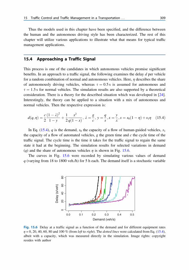
In Eq. (15.4), q is the demand, s0 the capacity of a flow of human-guided vehicles, s1the capacity of a flow of automated vehicles, g the green time and c the cycle time of thetraffic signal. The cycle time is the time it takes for the traffic signal to regain the samestate it had at the beginning. The simulation results for selected variations in demand(q) and the share of autonomous vehicles η is shown in Fig. 15.6.

The curves in Fig. 15.6 were recorded by simulating various values of demandq (varying from 18 to 1800 veh./h) for 5 h each. The demand itself is a stochastic variable

0.0 0.1 0.2 0.3 0.4 0.5

020

4060

80

Del

ay (

s/ve

h)

Demand (veh/s)

Fig. 15.6 Delay at a traffic signal as a function of the demand and for different equipment ratesη = 0, 20, 40, 60, 80 and 100 % (from left to right). The dotted lines were calculated from Eq. (15.4),albeit with a capacity, which was measured directly in the simulation. Image rights: copyrightresides with author

15 Traffic Control and Traffic Management in a Transportation … 309

(approximately Poisson-distributed), i.e. in each observed time interval, there is always adifferent number of vehicles and only the average over many such time intervals leads tothe correct demand.

The delay was recorded for each simulated vehicle and the values used to calculate theaverage entered in Fig. 15.6. In principle, the entire distribution of delays can be used tocharacterize the results, which for reasons of space is omitted here, although it would beinteresting. The fluctuations in the delays are a measure of the reliability of such a system.However, the example presented here shows that the delay fluctuations are only veryweakly correlated with the proportion of autonomously guided vehicles; the major source ofstochasticity in this system is generated by the demand and not the dynamics of the vehicles.

Two results in Fig. 15.6 stand out. For one thing, the description from the theory doesnot always correspond to the simulation results. A considerable amount of research is stillneeded here, because it’s not at all simple to translate the assumptions on which the theoryis based into the simulated reality. This will undoubtedly be even more difficult incomparison with real measured values. To achieve agreement, the values for thesaturation-traffic volume determined in the simulation had to be used—with the theoreticalvalues, i.e. the τ values defined in Sect. 15.3, the agreement is not compelling.

Second, autonomous vehicles “only” change the capacity; otherwise there are no oronly very small gains. As long as the demand stays away from the respective capacity,there are only minor differences between the various scenarios, at least on the level of thedescription selected here.

A change in the capacity does have one very positive effect, however: it means that therequired green times at a traffic signal can be shorter, leaving more time for other modes oftransport.

15.5 Adaptive Traffic Signals

Section 15.4 looked at a traffic signal with a fixed-time control system. Many modernsystems, however, utilize an adaptive control system. That means that the traffic signalattempts to coordinate its green times with the current demand. When demand is low, the

0 1 2 3 4

510

1520

2530

3540

Time (h)

Gre

en ti

me

(s)

0 1 2 3 4

050

100

150

200

Time (h)

Del

ay (

s/ve

h)

Fig. 15.7 Green times (left)and delays (right) in asimulated adaptive system,displayed as a function of thetime and for differentproportions of autonomousvehicles η = 0, 25, 50, 75,100 %. The demand parameterwas set to q0 = 180 veh./h andq1 = 720 veh./h. Image rights:copyright resides with author

310 P. Wagner

green times are short, and when demand is high, the system responds with long greentimes. The details are somewhat more complex, because the delay regarded as a functionof the demand has a minimum with a certain optimal cycle time. An adaptive system isable to choose the optimal cycle time for itself, and makes very clever use of the fluc-tuations that occur in the traffic flow.

In this case as well, the aim is to examine how such an adaptive system handles a mixof autonomous and normal vehicles. To this purpose, simulation of a two-armed inter-section controlled with an adaptive method was set up [27]. The two arms are 600 m long,and the delay per vehicle at intersection is measured. In contrast to Sect. 15.4, however, ademand was selected that depends on the time and thus replicates a peak hour group inwhich at the time of maximum demand the system is saturated in spite of its adaptivity.The demand function selected here is:

q tð Þ ¼ q0 þ q1 sinptT

� �;

where q0 is a basic load, q1 is the amplitude of the demand fluctuation and T is the entiretime period of the simulation. Both arms are subjected to the same demand, whichrepresents a relatively unfavorable case.

Beyond the delays, in this case it is primarily the green times that are of interest. Sincethe system adapts the times to the demand, they fluctuate within typical ranges. In manycountries, the green time cannot fluctuate freely: for instance, the green time for a normaltraffic signal cannot sink below 5 s, and in the following simulations, the maximum greentime is set to 40 s.

Such a simulation is also an interesting case in the evaluation of the simulation data.A single simulation of such a peak hour shows major fluctuations in terms of delays aswell as green time and cycle times. Although the delays were averaged over a cycle of thesystem, that in itself is not sufficient because the cycles are themselves stochastic variables

0 20 40 60 80

010

2030

40

Offset (s)

Del

ay (

s/ve

h)

Fig. 15.8 Delay as a function of the offset time for a simple green wave. Depicted here is asimulation with human drivers (gold) and one only with autonomous vehicles (blue). Shown here isthe best result achieved between the first and second intersection. Image rights: copyright resideswith author

15 Traffic Control and Traffic Management in a Transportation … 311

whose average values and statistics can only be determined through a sufficient number ofrepetitions of the same scenario with slightly different details—just as in reality whensuccessive days are examined. To obtain statistically valid results, in this case the peakhour was repeated 50 times. At 5-min intervals, the averages of the delays over the lastcycle and the corresponding green times set by the system were collected. The results inFig. 15.7 were composed from this data.

With maximum demand, the system extends the green times up to the limit of 40 s andthereby demonstrates that it has reached its saturation level. However, this only applies fora flow of normal vehicles. As soon as autonomous vehicles are added to the mix, the topdelay value for sinks and with an equipment rate of 50 %, the maximum green time is noteven reached. This lines up with the observation in Sect. 15.4 that autonomous vehiclesnot only increase the capacity, but also contribute to a reduction in green times—an effectthat is rather clear in this example, namely that even a small proportion of autonomouslyguided vehicles can make a noticeable impact.

15.6 Green Wave with Autonomous Vehicles

The previous scenarios examined a single intersection. Much more interesting is the caseof a stretch of road with multiple intersections in succession which are all controlled by atraffic signal system. In this case the coordination between the traffic signals, known

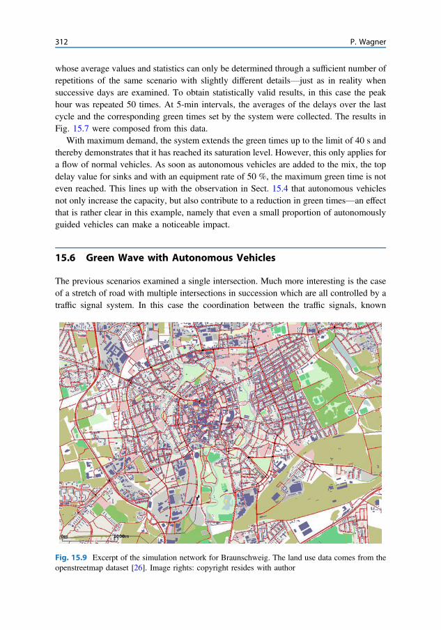
Fig. 15.9 Excerpt of the simulation network for Braunschweig. The land use data comes from theopenstreetmap dataset [26]. Image rights: copyright resides with author

312 P. Wagner

colloquially as the green wave, plays an important role. Here again, a simulation is used toinvestigate how great an impact the introduction of autonomous vehicles has. Analogousto the procedure in [28], a section of road with 10 intersections is simulated with varyingcoordination configurations. The demand, which is constant, the green times and the cycletimes remain unchanged. The only change is to the offset, i.e. the point in time at whichthe traffic signal turns green for the vehicle flow in a particular direction. If this offsetbetween two signals is precisely equal to the travel time between the two signals, thesystem is in its optimal state: the delay for the vehicles at the downstream signal is exactlyzero when the green times are equal. In that case, just as many vehicles can cross theintersection as left the upstream traffic signal.

The expectation is clear: In this case, no improvements will be achieved with anautonomous vehicle; and that is precisely what the simulation results in Fig. 15.8demonstrate. However, autonomous vehicles do indeed improve the delay times in thecase of sub-optimal coordination. The reason is that the bunch of vehicles that leaves atraffic signal is more compressed than with human drivers.

15.7 Simulation of a City

This final section will examine how the introduction of autonomous vehicles might impactan entire city. To this purpose, an existing SUMO simulation [19 25] of the city ofBraunschweig is used to simulate the impact of autonomous vehicles on the traffic flow ofa transportation system.

However, the model introduced in Sect. 15.2 is not implemented in SUMO, so thesimulation has to be carried out with the models that are available in SUMO. The sim-ulation therefore uses the standard model integrated in SUMO, which in terms ofdescribing the fluctuations of the drivers is not as refined as the model introduced here.

0 5 10 15 20

020

4060

8012

014

010

0

Time (h)

Del

ay (

s/ve

h)

Fig. 15.10 Comparison of the delays for a simulation with human drivers (gold, upper curve) and asimulation in which the passenger vehicles drive autonomously (blue, lower curve). Each data pointis a floating average value from the 8 adjacent one-minute values. The dispersion of the values of thetwo curves is not very different and is therefore not displayed. Image rights: copyright resides withauthor

15 Traffic Control and Traffic Management in a Transportation … 313

To set up the model, a modified network by the NavTeq company is used; an extract ofthe transportation network is seen in Fig. 15.9. The full simulation comprises the entirearea of the city of Braunschweig, including the autobahns in the area. The simulationnetwork comprises approximately 129,000 edges.

The required traffic demand comes from a start/destination matrix from the PTVcompany, which is available for different days of the week in 24 time slices of one houreach for each of those days. This demand was used to calculate a user equilibrium, whichin this case required some 100 iteration steps. At the end of this process, for each vehiclesimulated in SUMO there is an optimal route in the sense that every other route throughthe network would take longer. A total of 647,000 vehicles were simulated. Initialcomparisons with real data from Braunschweig suggest that the matrix significantlyunderestimates the demand. This undoubtedly affects the results discussed here, but it wasnot possible to carry out such corrections in the context of this project.

To simulate autonomous vehicles, a new vehicle type is introduced which has similarparameters to the models in Sect. 15.2: the autonomous vehicles in SUMO drive withτ = 0.5 s, all others with τ = 1 and σ = 0.5. σ is the noise parameter in SUMO, i.e. itindicates by how much a vehicle deviates from the optimal driving style. The selection ofτ = 0.5 s means that the time-step size in SUMO also has to be set to 0.5 s to ensure thatthe vehicles can continue to drive without colliding. This extends the simulation time fromaround 50 min to 90 min for the simulation of an entire day in Braunschweig.

Only the passenger vehicles were simulated as autonomous vehicles; the approximately44,000 trucks remained unchanged. The traffic signals were likewise not entirely correctlyrepresented in the simulation. It may therefore be assumed that on this end as well, furthercorrections to the simulation results below can be expected.

Nevertheless, this simulation delivers significant preliminary results, as seen inFig. 15.10. Even without further measures, the autonomous system is more efficient in thesense that it reduces delays between 5 and 80 %, with an average value of around 40 %.With the selected parameters, however, the variance in travel times changes relativelylittle; the system, in other words, becomes faster, but not necessarily more reliable. Thatcould change if the traffic management system were also realistically simulated. Suchstudies are currently in the works.

15.8 Conclusion

This paper presents some initial considerations regarding how traffic management needs torespond to the opportunities presented by autonomous driving. The case studies presentedhere demonstrate that, depending on the scenario, very different improvements can beachieved in the flow of traffic through the introduction of autonomous vehicles.

Unfortunately, the improvements that could be achieved are difficult to summarize witha single number. It was demonstrated in Sect. 15.4, for example, that the capacity of atraffic signal can certainly be doubled. If the demand is low at the corresponding signal,

314 P. Wagner

this doubling is scarcely noticeable. But if the signal is working at the limits of itscapacity, by contrast, even a minor increase in its capacity can lead to a dramaticimprovement.

This can be observed quite clearly in the scenario in Sect. 15.5: here the demand runsthe values from very low to (temporary) over-saturation. Although the introduction ofautonomous vehicles has little impact on green times and delays when demand is low, ityields major improvements when the system is operating beyond capacity. Nevertheless,the magnitude of these improvements does depend on the details of the scenario beingexamined. If the peak value for demand were just a bit lower, the benefit would also besignificantly diminished.

That notwithstanding, it may be asserted with confidence that at least in the urbancontext, the introduction of autonomous vehicles has the potential to generate substantialtime gains at traffic signals which would then be available for other road users—if theintroduction of these vehicles does not lead to an increase in demand for automotivetransportation.

Open Access This chapter is distributed under the terms of the Creative Commons Attribution 4.0International License (http://creativecommons.org/licenses/by/4.0/), which permits use, duplication,adaptation, distribution and reproduction in any medium or format, as long as you give appropriate creditto the original author(s) and the source, a link is provided to the Creative Commons license and anychanges made are indicated.

The images or other third party material in this chapter are included in the work’s Creative Commonslicense, unless indicated otherwise in the credit line; if such material is not included in the work’s CreativeCommons license and the respective action is not permitted by statutory regulation, users will need toobtain permission from the license holder to duplicate, adapt or reproduce the material.

References

1. Winner, H.: private correspondence. (2014)2. Friedrich, B.: The Effect of Autonomous Vehicles on Traffic. Present volume (2014)3. Pavone, M.: The Value of Robotic Mobility-on-Demand Systems. Present volume (2014)4. van Dijke, J., van Schijndel, M., Nashashibi, F., de la Fortelle, A.: Certification of Automated

Transport Systems. Procedia - Social and Behavioral Sciences 48, 3461 – 3470 (2012)5. Kesting, A.: Microscopic Modeling of Human and Automated Driving: Towards

Traffic-Adaptive Cruise Control, Verlag Dr. Müller, Saarbrücken, ISBN 978-3-639-05859-8(2008)

6. Reuschel, A.: Fahrzeugbewegung in der Kolonne bei gleichförmig beschleunigtem oderverzögertem Leitfahrzeug. Zeitschrift des österreichischen Ingenieur und Architektenvereins,7/8, 95 – 98 (1950)

7. Chowdhury, D., Santen, L., Schadschneider, A.: Statistical physics of vehicular traffic and somerelated systems. Physics Reports 329, 199 – 329 (2000)

8. Helbing, D.: Traffic and Related Self-Driven Many-Particle Systems. Reviews of ModernPhysics 73, 1067 – 1141 (2001)

9. Nagel, K., Wagner, P., Woesler, R.: Still flowing: approaches to traffic flow and traffic jammodelling. Operations Research 51, 681 – 710 (2003)

10. Treiber, M., Kesting, A.: Traffic Flow Dynamics: Data, Models and Simulation. (2012)

15 Traffic Control and Traffic Management in a Transportation … 315

11. Urmson C., et al: Autonomous Driving in Urban Environments: Boss and the Urban Challenge.Journal of Field Robotics 25, 425 – 466 (2008)

12. Levinson, J. et al.: Towards fully autonomous driving: Systems and algorithms. In proceedingsof the 2011 IEEE Intelligent Vehicles Symposium, 163 – 168 (2011)

13. Campbell M., Egerstedt, M., How, J. P., Murray, R. M.: Autonomous driving in urbanenvironments: approaches, lessons and challenges. Philosophical Transactions of the RoyalSociety A 368, 4649 – 4672 (2010)

14. Winner, H., Hakuli, S., Wolf, G.: Handbuch Fahrerassistenzsysteme: Grundlagen,Komponenten und Systeme für aktive Sicherheit und Komfort (2011)

15. Helly, W.: Simulation of bottlenecks in single lane traffic flow. Proceedings of the symposiumon theory of traffic flow (1959)

16. Gipps, P.: A behavioural car-following model for computer simulation. Transportation ResearchPart B 15, 105 – 111 (1981)

17. Krauß, S.: Microscopic modelling of traffic flow: Investigation of Collision Free VehicleDynamics, Dissertation, Universität zu Köln (1998)

18. Krauß, S., Wagner, P., Gawron, C.: Metastable states in a microscopic model of traffic flow.Physical Review E 55, 5597 – 5602 (1997)

19. Krajzewicz, D, Erdmann, J., Behrisch, M, Bieker, L.: Recent Development and Applications ofSUMO - Simulation of Urban MObility. International Journal On Advances in Systems andMeasurements, 5, 128 – 138 (2012)

20. Wagner, P.: Analyzing fluctuations in car-following. Transportation Research Part B 46, 1384 –

1392 (2012)21. Jiang, R., Hu, M., Zhang, H.M., Gao, Z., Jia, B., Wu, Q., Wang, B., Yang, M.: Traffic

Experiment Reveals the Nature of Car-Following. PLoS ONE 9: e94351. doi:10.1371/journal.pone.0094351 (2014)

22. Todosiev, E.P., L. C. Barbosa, L.C.: A proposed model for the driver-vehicle-system. TrafficEngineering, 34, 17 – 20, (1963/64)

23. Wagner, P.: A time-discrete harmonic oscillator model of human car-following. EuropeanPhysical Journal B 84, 713 – 718 (2011)

24. Webster, F.V.: Traffic Signal Settings. Department of Scientific And Industrial Research RoadResearch Laboratory, (1958)

25. Krajzewicz, D., Furian, N., Tomàs Vergés, J.: Großflächige Simulation vonVerkehrsmanagementansätzen zur Reduktion von Schadstoffemissionen. 24.Verkehrswissenschaftliche Tage Dresden, Deutschland (2014)

26. OpenStreetMap: www.openstreetmap.org, last accessed 7/29/201427. Oertel, R., Wagner, P.: Delay-Time Actuated Traffic Signal Control for an Isolated Intersection.

In: Proceedings 90th Annual Meeting Transportation Research Board (TRB) (2011)28. Gartner, N.H., Wagner, P.: Traffic flow characteristics on signalized arterials. Transportation

Research Records 1883, 94 – 100 (2004)

316 P. Wagner